The Dynamic Migration Game:A Structural Econometric Model and Application to Rural Mexico∗

Ruben Irvin Rojas Valdes, C.-Y. Cynthia Lin Lawell, and J. Edward Taylor

Abstract

The migration decisions of households in a village can be thought of as a dynamicgame in which each household makes decisions about how to allocate its members acrossdistinct activities, taking into account dynamic considerations about the future and strate-gic considerations about what other households in the village are doing. We develop andestimate a structural econometric model of this dynamic migration game, and apply itto households in rural Mexico. We use the estimated parameters to simulate the effectsof counterfactual policy scenarios, including those regarding wages, government policy,schooling, crime rates at the border, and precipitation, on migration decisions and wel-fare. Results show that analyses that ignore the possibility of strategic interactions ordynamic behavior lead to misleading results. In addition, owing in part to strategic in-teractions and dynamic behavior, a cap on total migration to the US decreases migrationnot only to the US but also within Mexico as well, causes migration to the US to de-crease by more than what is required by the policy, and decreases average welfare perhousehold-year.

JEL Codes: O15, O54Keywords: migration, Mexico, strategic interactions, dynamic behavior, dynamic game,structural econometric modelThis draft: July 2018

∗Rojas Valdes: University of California at Davis; rirojas@ucdavis.edu. Lin Lawell: Cornell University. Taylor: University ofCalifornia at Davis. We thank Aaron Adalja, Max Auffhammer, Arnab Basu, Tim Beatty, Steve Boucher, Christine Braun, ColinCarter, Michael Carter, John Cawley, Yang-Ming Chang, Yuan Chen, Ian Coxhead, Andres Cuadros, Gordon Dahl, Kaniska Dam,Giuseppe De Arcangelis, Laura Dick, Sonia DiGiannatale, Alexander Elbittar, Nilesh Fernando, Oleg Firsin, Arya Gaduh, KajalGujati, Emilio Gutierrez, Maulik Jagnani, Tu Jarvis, Nancy Jianakoplos, Diego Jimenez, Michael Kremer, David R. Lee, AlejandroLopez-Feldman, Travis Lybbert, Jonathan Malacarne, Fernanda Marquez, William Masters, Shaun McRae, Pierre Merel, ErichMuehlegger, Esteban Quinones, Hillel Rapoport, John Rust, Stephen Ryan, Louis Sears, Ashish Shenoy, Ellis Tallman, RandellTorno, Diego Ubfal, Kurt Unger, Arthur van Benthem, Bruce Wydick, Jianwei Xing, and Jisang Yu for invaluable comments anddiscussions. We benefited from comments from seminar participants at Cornell University, Centro de Investigacion y DocenciaEconomicas (CIDE), the University of San Francisco, the University of California at Davis, and the Gifford Center for PopulationStudies; and from conference participants at the Latin American Meeting of the Econometric Society (LAMES); the OxfordSymposium on Population, Migration, and the Environment; the Pacific Conference for Development Economics; the MidwestInternational Economic Development Conference; the CIRET International Conference on Migration and Welfare; the North EastUniversities Development Consortium Conference (NEUDC); the Western Economic Association International (WEAI) GraduateStudent Dissertation Workshop; and the Agricultural and Applied Economics Association Annual Meeting. We thank GerardoAragon, Diane Charlton, Katrina Jessoe, Rebecca Lessem, and Dale Manning for their help with the data. We are also indebtedto Antonio Yunez-Naude and the staff of PRECESAM and of Desarrollo y Agricultura Sustentable for their invaluable assistanceand data support. We received financial support from the University of California Institute for Mexico and the United States(UC MEXUS), a Gifford Center Travel Award, a UC-Davis Graduate Student Travel Award, and a Cornell University DEEP-GREEN-RADAR Travel Award. Lin Lawell is a former member and Taylor is a member of the Giannini Foundation of AgriculturalEconomics. All errors are our own.

1 Introduction

According to estimates from the World Bank (2010a), around 3 percent of the world popula-

tion live in a country different from the one in which they were born. The US is the country

with the highest immigrant population in the world, with more than 46 million people who

were foreign born (United Nations, 2013), of which about 11 million are from Mexico (World

Bank, 2010b). These trends are considerably changing demographic portraits, reshaping

patterns of consumption, and altering the cultures of both sending and receiving countries

(Rojas Valdes, Lin Lawell and Taylor, 2018).

Given the economic significance of migration and its relevance for policy (Rojas Valdes,

Lin Lawell and Taylor, 2018), it is important to understand the factors that cause people to

migrate. We add to the literature on the determinants of migration by incorporating two

important features of migration decisions: strategic interactions and dynamic behavior.

Migration decisions are dynamic because households consider the future when making

these decisions, basing them not only on the current state of economic factors, but also on the

prospects of economic opportunities in other areas and the potential streams of net benefits

(or payoffs) from migrating. Migration decisions are also dynamic because these decisions

can be viewed as forms of investment that are made under uncertainty. Migration decisions

are at least partially irreversible, there is leeway over the timing of these decisions, and the

payoffs from these decisions are uncertain; as a consequence, there may be an option value

to waiting before making these decisions that makes these decisions dynamic rather than

static (Dixit and Pindyck, 1994).

In addition to being dynamic, migration decisions are also strategic. We define ’strategic

interactions’ as arising whenever the migration decisions of other households in the village

affect a household’s payoffs from migration and therefore its decisions to have a member

migrate. There are several reasons why a household’s migration decisions may depend on the

migration decisions of its neighbors, including migration networks, information externalities,

relative deprivation, risk sharing, competition effects (Rojas Valdes, Lin Lawell and Taylor,

2018), a limited number of employers at the destination site who do not discriminate against

migrants from elsewhere (Carrington, Detragiache and Vishwanath, 1996), the marriage

market (Riosmena, 2009), and cultural norms (Kandel and Massey, 2002). Our structural

model is general enough to capture multiple possible sources of strategic interactions, and

enables us to analyze their net effect.1

1We choose to use the term ’strategic interactions’ instead of ’peer effects’ for two main reasons. First,the term ’peer’ often connotes an individual; in contrast; the decision-makers we examine are householdsrather than individuals. Second, a possible source of strategic interactions we allow for in our analysis is acompetition effect, which is an effect that is potentially more accurately described as a ’strategic interaction’

1

Owing to strategic interactions and dynamic behavior, the migration decisions of house-

holds in a village can be thought of as a dynamic game in which each household makes

decisions about how to allocate its members across distinct activities, taking into account dy-

namic considerations about the future and strategic considerations about what other house-

holds in the village are doing. We develop and estimate a structural econometric model of

this dynamic migration game.

We build on the previous literature on the determinants of migration by estimating a

structural econometric model that incorporates strategic interactions and dynamic behavior,

and that enables us to calculate welfare and to analyze the effects of counterfactual scenarios

on decisions and welfare. Furthermore, the previous literature on migration externalities

focuses primarily on externalities that arise at the destination site, including, for example,

migration networks. Our research fills a gap in the literature by accounting for migration

externalities that occur in the source country in the form of strategic interactions, and by

incorporating these strategic interactions in a dynamic setting.

There are several advantages to using a dynamic structural econometric model. First,

a dynamic structural model explicitly models the dynamics of migration decisions. Second,

a dynamic structural model incorporates continuation values that explicitly model how ex-

pectations about future affect current decisions. Third, a structural econometric model of

a dynamic game enables us to estimate structural parameters of the underlying dynamic

game with direct economic interpretations. These structural parameters include parameters

that measure the effects of state variables on household payoffs (utility) and the net effect of

the strategic interactions. These parameters account for the continuation value. Fourth, the

parameter estimates can be used to calculate welfare. Fifth, the parameter estimates can be

used to simulate the effects of counterfactual scenarios on decisions and welfare.2

Our structural econometric model of the dynamic migration game enables us to exam-

ine how natural factors, economic factors, institutions, government policies, and strategic

rather than a ’peer effect’. Nevertheless, our concept of ’strategic interactions’ is very similar to that of ’peereffects’.

2A potential drawback of structural econometric models is that they require sources of structure (e.g.,from economic theory), and the assumptions underlying these sources of structure may or may not holdin reality. We mitigate these concerns by imposing minimal, parsimonious assumptions in our structuraleconometric model of the dynamic migration game. As we explain in more detail in our description of ourmodel, the sources of economic structure in our structural econometric model of the dynamic migrationgame are dynamic programming and game theory. Aside from dynamic programming and game theory,we impose minimal additional assumptions on our model. For example, our specification of the per-periodpayoff function is agnostic about the actual functional form of the utility function, the actual nature ofthe constraints, the actual economic and non-economic channels through which migration affects householdutility, and the actual mechanisms by which state variables such as local wages affect utility, and thusis general enough to capture the reduced-form implications of a number of models of general equilibriumbehavior of individuals within the household, households in the village, and the village economy.

2

interactions affect the migration decisions of households in rural Mexico. We use the esti-

mated parameters to simulate the effects of counterfactual policy scenarios, including those

regarding wages, government policy, schooling, crime rates at the border, and precipitation,

on migration decisions and welfare. In order to disentangle the effects of strategic interac-

tions and dynamic behavior in our model, we also simulate counterfactual scenarios in which

remove strategic interactions, and counterfactual scenarios in which we remove dynamic

behavior.

Results show that analyses that ignore the possibility of strategic interactions or dynamic

behavior lead to misleading results. In addition, owing in part to strategic interactions and

dynamic behavior, a cap on total migration to the US decreases migration not only to the US

but also within Mexico as well, causes migration to the US to decrease by more than what

is required by the policy, and decreases average welfare per household-year. Thus, not only

do barriers to migration from Mexico to the U.S. have no positive effect on U.S. agricultural

wages or employment (Clemens, Lewis and Postel, 2017), but our results show that such

barriers to migration decrease the average welfare of households in rural Mexico.

The balance of the paper is as follows. Section 2 reviews the related literature on mi-

gration and structural econometric models. Section 3 presents our model of the dynamic

migration game. Section 4 describes the econometric estimation. Section 5 provides back-

ground information on the importance of migration in rural Mexico and describes the data.

Section 6 presents the results of the structural econometric model. Section 7 presents the

results of our counterfactual simulations. Section 8 concludes.

2 Literature Review

2.1 Determinants of Migration

The first strand of literature upon which our paper builds is the literature on determinants of

migration. The new economics of labor migration posits the household as the relevant unit

of analysis. Using the household as the relevant unit of analysis addresses several observed

features of migration that are ignored by individualistic models, including the enormous flows

of remittances and the existence of extended families which extend beyond national borders.

Most applications of the new economics of labor migration assume that the preferences of

the household can be represented by an aggregate utility function and that income is pooled

and specified by the household budget constraint.

For example, Stark and Bloom (1985) assume that individuals with different preferences

and income not only seek to maximize their utility but also act collectively to minimize risks

3

and loosen constraints imposed by imperfections in credit, insurance, and labor markets.

This kind of model assumes that there is an informal contract among members of a family

in which members work as financial intermediaries in the form of migrants. The household

acts collectively to pay the cost of migration by some of its members, and in turn migrants

provide credit and liquidity (in form of remittances), and insurance (when the income of

migrants is not correlated with the income generating activities of the household). In this

setting, altruism is not a precondition for remittances and cooperation, but it reinforces the

implicit contract among household members (Taylor and Martin, 2001). In their analysis

of how migration decisions of Mexican households respond to unemployment shocks in the

US, Fajardo, Gutierrez and Larreguy (2017) emphasize the role played by the household,

as opposed to individuals, as the decision-making unit at the origin. Garlick, Leibbrandt

and Levinsohn (2016) provide a framework with which to analyze the economic impact of

migration when individuals migrate and households pool income.

In the new economics of labor migration, individual characteristics and human capital

variables are also very important because they influence both the characteristics of the

migrants and the impacts that migration has on the productive activities of the remaining

household. Human capital theory a la Sjaastad (1962) suggests that migrants are younger

than those who stay because younger migrants would capture the returns from migration

over a longer time horizon. The role of education depends on the characteristics of the host

and the source economy. Education is positively related to rural-urban migration but has

a negative effect on international migration (Taylor, 1987). The reason is that education

is not equally rewarded across different host economies. For example, agricultural work in

the United States requires only low-skilled labor, so education has a negative effect on the

selection of migrants for this type of work.

Changes in labor demand in the United States has modified the role of migrant char-

acteristics in determining who migrates. Migrants from rural Mexico, once mainly poorly

educated men, more recently have included female, married, and better educated individ-

uals relative to the average rural Mexican population (Taylor and Martin, 2001). Borjas

(2008) finds evidence that Puerto Rico migrants to the United States have lower incomes,

which is consistent with Borjas’ (1987) prediction that migrants have incomes lower than

the mean income in both the source and host economies when the source economy has low

mean wages and high inequality. On the other hand, Feliciano (2001), Chiquiar and Hanson

(2005), Orrenius and Zavodny (2005), McKenzie and Rapoport (2010), Cuecuecha (2005),

and Rubalcaba et al. (2008) find that Mexican migrants come from the middle of the wage

or education distribution. McKenzie and Rapoport (2007) show that migrants from regions

with communities of moderate size in the United States come from the middle of the wealth

4

distribution, while migrants from regions with bigger communities in the United States come

from the bottom of the wealth distribution.

The financial costs of migration can be considerable relative to the income of the poorest

households in Mexico.3 Angelucci (2015) finds that financial constraints to international

migration are binding for poor Mexicans, some of whom would like to migrate but cannot

afford to. Migration costs reflect in part the efforts of the host country to impede migration,

which might explain why migration flows continue over time and why we do not observe

enormous flows of migrants (Hanson, 2010). Migration costs for illegal crossing from Mexico

to the United States are estimated to be 2,750 to 3,000 dollars (Mexican Migration Program,

2014). Estimates reported in Hanson (2010) suggest that the cost of the “coyote” increased

by 37 percent between 1996-1998 and 2002-2004, mainly due to the increase of border en-

forcement due to the terrorist attacks of 9/11. Nevertheless, Gathmann (2008) estimates

that even when the border enforcement expenditure for the Mexico-United States border

almost quadrupled between 1986 and 2004, the increase in expenditure produced an increase

the cost of the coyote of only 17 percent, with almost zero effect on coyote demand.

Migration decisions may also be affected by weather and climate. Jessoe, Manning and

Taylor (2018) evaluate the effects of annual fluctuations in weather on employment in rural

Mexico to gain insight into the potential labor market implications of climate change, and

find that extreme heat increases migration domestically from rural to urban areas and in-

ternationally to the U.S. Feng, Krueger and Oppenheimer (2010) find a significant effect of

climate-driven changes in crop yields on the rate of migration from Mexico to the United

States. Maystadt, Mueller and Sebastian (2016) investigate the impact of weather-driven

internal migration on labor markets in Nepal. Mason (2016) analyzes climate change and

migration using a dynamic model, and shows that the long run carbon stock, and the en-

tire time path of production (and hence emissions), is smaller in the presence of migration.

Mahajan and Yang (2017) find that hurricanes in source countries increase migration to the

U.S., with the effect increasing in the size of prior migrant stocks.

The previous literature on migration externalities focuses primarily on externalities that

arise at the destination site, including, for example, migration networks. Our research fills a

gap in the literature by accounting for migration externalities that occur in the source country

in the form of strategic interactions, and by incorporating these strategic interactions in a

dynamic setting.

We build on our analysis in Rojas Valdes, Lin Lawell and Taylor (2018), in which we

3Data from the National Council for the Evaluation of the Social Policy in Mexico (CONEVAL) showthat the average income of the poorest 20 percent of rural Mexican households was only 456 dollars a yearin 2012.

5

estimate reduced-form models to analyze strategic interactions, or ’neighborhood effects’, in

migration decisions. Using instrumental variables to address the endogeneity of neighbors’

decisions, we empirically examine whether strategic interactions in migration decisions ac-

tually take place in rural Mexico, whether the interactions depend on the size of the village,

and whether there are nonlinearities in the strategic interactions (Rojas Valdes, Lin Lawell

and Taylor, 2018).

We build on the previous literature on the determinants of migration by estimating a

structural econometric model that incorporates both dynamic behavior and strategic inter-

actions, and that enables us to calculate welfare and to analyze the effects of counterfactual

scenarios on decisions and welfare.

2.2 Structural econometric models

In addition to the literature on migration, our paper also builds on previous literature using

structural econometric models.

There is a burgeoning literature using structural models in development economics.

Shenoy (2016) estimates the cost of migration and migration-related supply elasticity in

Thailand using structural model of location choice. He finds that the costs of migration are

0.3 to 1.1 times as high as average annual earnings. He also finds that migration contributes

8.6 percentage points to local labor supply elasticity. We build on Shenoy’s (2016) work by

explicitly modeling the dynamic and strategic components of international migration.

To explain the large spatial wage disparities and low male migration in India, Munshi

and Rosenzweig (2016) develop and estimate a structural econometric model of the trade-

off between consumption smoothing, provided by caste-based rural insurance networks, and

the income gains from migration. We build on Munshi and Rosenzweig’s (2016) work by

explicitly modeling the dynamics of international migration, by allowing for multiple channels

of strategic interactions in addition to networks, and by applying our model to migration

from rural Mexico.

The seminal work of Rust (1987), who develops an econometric method for estimating

single-agent dynamic discrete choice models, is the cornerstone of dynamic structural econo-

metric models. Structural econometric models of dynamic behavior have been applied to

model bus engine replacement (Rust, 1987), nuclear power plant shutdown decisions (Roth-

well and Rust, 1997), water management (Timmins, 2002), air conditioner purchase behavior

(Rapson, 2014), copper mining decisions (Aguirregabiria and Luengo, 2016), wind turbine

shutdowns and upgrades (Cook and Lin Lawell, 2018), agricultural disease management

(Carroll et al., 2018b), supply chain externalities (Carroll et al., 2018a), agricultural produc-

6

tivity (Carroll et al., forthcoming), pesticide spraying decisions (Sambucci, Lin Lawell and

Lybbert, 2018), and decisions regarding labor supply, job search, and occupational choices

(see Keane, Todd and Wolpin, 2011).

Morten (2016) develops and estimates a dynamic structural model of risk sharing with

limited commitment frictions and endogenous temporary migration to understand the joint

determination of migration and risk sharing in rural India. We build on Morten’s (2016)

work by allowing for multiple channels of strategic interactions in addition to risk sharing,

and by applying our model to migration from rural Mexico.

As many migrations are temporary (Dustmann and Gorlach, 2016), Kennan and Walker

(2011) estimate a dynamic structural econometric model of optimal sequences of migration

decisions in order to analyze the effects of expected income on individual migration decisions.

They apply the model to interstate migration decisions within the United State. The model

is estimated using panel data from the National Longitudinal Survey of Youth on white

males with a high-school education. Their results suggest that the link between income

and migration decisions is driven both by geographic differences in mean wages and by a

tendency to move in search of a better locational match when the income realization in the

current location is unfavorable.

While most of the dynamic structural econometric models in development economics

model single-agent dynamic decision-making (see e.g., Todd and Wolpin, 2010; Duflo, Hanna

and Ryan, 2012; Mahajan and Tarozzi, 2011), we model a dynamic game between decision-

makers, and thus allow for both dynamic and strategic decision-making.

Structural econometric models of dynamic games include a model developed by Pakes,

Ostrovsky and Berry (2007), which has been applied to the multi-stage investment timing

game in offshore petroleum production (Lin, 2013), to ethanol investment decisions (Thome

and Lin Lawell, 2018), and to the decision to wear and use glasses (Ma, Lin Lawell and

Rozelle, 2018); and a model developed by Bajari et al. (2015), which has been applied to

ethanol investment (Yi and Lin Lawell 2018a; Yi and Lin Lawell, 2018b). Structural econo-

metric models of dynamic games have also been applied to fisheries (Huang and Smith, 2014),

dynamic natural monopoly regulation (Lim and Yurukoglu, 2018), and Chinese shipbuilding

(Kalouptsidi, 2018).

The structural econometric model of a dynamic game we use is based on a model devel-

oped by Bajari, Benkard and Levin (2007), which has been applied to the cement industry

(Ryan, 2012; Fowlie, Reguant and Ryan, 2016), the ethanol industry (Yi, Lin Lawell and

Thome, 2018), the world petroleum industry (Kheiravar, Lin Lawell and Jaffe, 2018), cli-

mate change policy (Zakerinia and Lin Lawell, 2018), and the global market for solar panels

(Gerarden, 2018).

7

3 Dynamic Migration Game

We model the migration decisions of households in a village as a dynamic game in which

each household makes decisions about how to allocate its members across distinct activities,

taking into account dynamic considerations about the future and strategic considerations

about what neighbors in the village are doing.

The players i = 1, ..., N in our dynamic migration game are households within a village.

Each year t = 1, ...,∞, each household i chooses an action from a discrete finite set ait ∈ Ai,

and all households in the village choose their time-t actions ait simultaneously, such that

at = (a1t, ..., aNt) ∈ A summarizes the actions played at t.

In our model, the actions are whether to engage in migration to the US, and whether

to engage in migration within Mexico. We do not assume that the actions are mutually

exclusive, so it is possible for a household to engage in both migration to the US and

migration within Mexico at the same time. Thus, in each year t, each household i decides

whether to send individual members to migrate to the US and/or to other areas within

Mexico, while also keeping some members in the village.

The vector of state variables at time t is given by st ∈ S ⊂ RL. State variables include

natural factors, economic factors, and government policy.

The state variables at the household level in sit include the number of males in the

household, the age of the household head; the schooling of the household head; the maximum

level of schooling achieved by any of the household members; the average level of schooling,

measured as the number of years of education that have been completed, of household

members 15 years old and above; a dummy if the household’s first born was a male; the

slope and quality of land owned by the household that is irrigated for agricultural purposes,

interacted with village precipitation; whether the household engaged in migration to the US

the previous year; and whether the household engaged in migration within Mexico in the

previous year. The slope and quality of household land interacted with contemporaneous

precipitation captures shocks to agricultural home production and therefore to household

income that vary by household and year and that may affect migration decisions.

The state variables at the municipality level in sit include the number of schools in the

basic system, the number of schools in the indigenous system, the number of cars, and the

number of buses. The state-level variables in sit include employment by sector. The national

variables in sit are aggregate variables that represent the broad state of the institutional and

economic environment relevant for migration, including the average hourly wage, and wage

by sector. The border crossing variables in sit includes variables that measure crime, deaths,

and border enforcement at nearby border crossing points.

8

Each period t, each household i receives an idiosyncratic private information shock

εit ∈ Ei independent of other players’ private shock with distribution Gi(·|st) such that

the collection of idiosyncratic shocks is εt = (ε1t, ..., εNt). The private information shocks

may represent, for example, shocks to household costs, health, and/or income.

The per-period payoff to each household i, which measures the household i’s utility in a

given period t, depends on the actions ait played by household i, the actions a−it played by

other households, the state variables st, and household i’s private shock εit. The per-period

payoff (or utility) to a household includes anything and everything the household may care

about, including both economic and non-economic sources of utility. Our model therefore

captures both economic and non-economic motives for migration.

Our action variables are whether to engage in migration to the US, and whether to

engage in migration within Mexico. For the actions of neighbors, we include the fraction

of neighbors with migration to the US and the fraction of neighbors with migration within

Mexico.

The state variables we use in the per-period payoff function include the number of house-

hold members; the household head age; a dummy whether the first born child of the house-

hold was male; household head schooling; household average schooling; household land qual-

ity interacted with rain; the number of basic schools; the hourly wage; the distance to the

closest border crossing point; and the crime rate at the closest, second closest, and third

closest border crossing points.

We assume that the payoff function is indexed by a finite parameter vector θ, so that the

payoff function is given by πi(a, s, εi; θ). The parameters θ to be estimated are the coefficients

on the terms in the per-period payoff function, which include terms that are functions of

action variables, strategic variables, demographic characteristics of the household, natural

factors, economic factors, and government policies. In particular, the terms in the per-period

payoff function include terms for each of the state variables; terms for the state variables

squared; and terms that interact each state variable, including the strategic variables, with

the household’s own action variables.

The payoff function is the per-period payoff for each household. While the parameters θ

are common to all households, the values of the action variables, state variables, and private

information shocks vary by household; as a consequence, the per-period payoff is specific to

and varies for each household.4

We account for the important factors in a household’s utility maximization decision by

4We do not aggregate all households into a single utility function (although we do aggregate all membersof a household into the household’s utility function), nor is the payoff function for an “average” householdonly. Instead, the payoff function is the per-period payoff specific to each household, and the per-periodpayoff to each household depends on the actions played by all households.

9

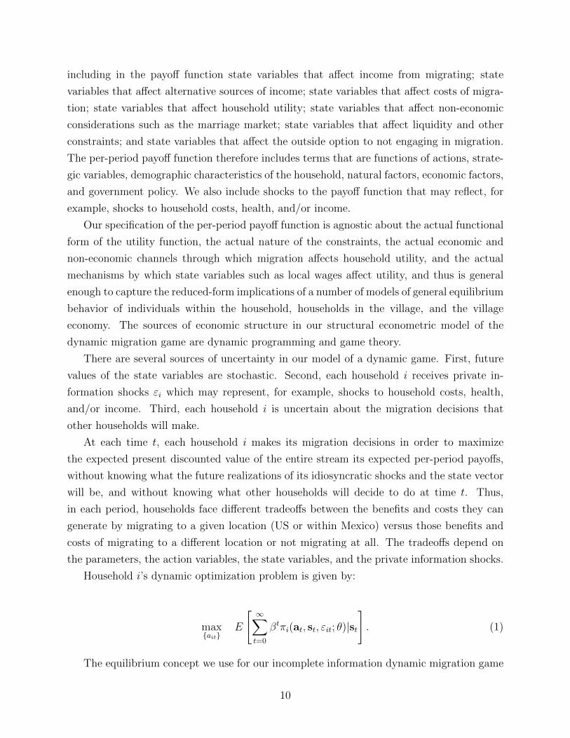
including in the payoff function state variables that affect income from migrating; state

variables that affect alternative sources of income; state variables that affect costs of migra-

tion; state variables that affect household utility; state variables that affect non-economic

considerations such as the marriage market; state variables that affect liquidity and other

constraints; and state variables that affect the outside option to not engaging in migration.

The per-period payoff function therefore includes terms that are functions of actions, strate-

gic variables, demographic characteristics of the household, natural factors, economic factors,

and government policy. We also include shocks to the payoff function that may reflect, for

example, shocks to household costs, health, and/or income.

Our specification of the per-period payoff function is agnostic about the actual functional

form of the utility function, the actual nature of the constraints, the actual economic and

non-economic channels through which migration affects household utility, and the actual

mechanisms by which state variables such as local wages affect utility, and thus is general

enough to capture the reduced-form implications of a number of models of general equilibrium

behavior of individuals within the household, households in the village, and the village

economy. The sources of economic structure in our structural econometric model of the

dynamic migration game are dynamic programming and game theory.

There are several sources of uncertainty in our model of a dynamic game. First, future

values of the state variables are stochastic. Second, each household i receives private in-

formation shocks εi which may represent, for example, shocks to household costs, health,

and/or income. Third, each household i is uncertain about the migration decisions that

other households will make.

At each time t, each household i makes its migration decisions in order to maximize

the expected present discounted value of the entire stream its expected per-period payoffs,

without knowing what the future realizations of its idiosyncratic shocks and the state vector

will be, and without knowing what other households will decide to do at time t. Thus,

in each period, households face different tradeoffs between the benefits and costs they can

generate by migrating to a given location (US or within Mexico) versus those benefits and

costs of migrating to a different location or not migrating at all. The tradeoffs depend on

the parameters, the action variables, the state variables, and the private information shocks.

Household i’s dynamic optimization problem is given by:

max{ait}

E

[∞∑t=0

βtπi(at, st, εit; θ)|st

]. (1)

The equilibrium concept we use for our incomplete information dynamic migration game

10

is that of a Markov Perfect Nash Equilibrium. A Markov state-space strategy for player i is

a function σi : S × Ei → Ai that maps combinations of state-shocks into actions such that

σ : S × E1 × ... × EN → A is the profile of strategies, and where Ei ⊂ RM is the support

of Gi. For a realization of the state vector s, the expected payoff of player i from playing

strategy σi is:

Vi(s;σ; θ) = Eε

[πi(σ(s, ε), s, εi; θ) + β

∫Vi(s

′;σ; θ)dP (s′|σ(s, ε), s)|s]. (2)

In a Markov Perfect Nash Equilibrium, the expected present discounted value that each

household i receives from playing its equilibrium strategy σi is at least as high as the expected

present discounted value it could receive from playing any other alternative strategy σ′i:

Vi(s;σ; θ) ≥ Vi(s;σ′i, σ−i; θ). (3)

4 Econometric Model

Finding a single equilibrium is computationally costly even for problems with a simple struc-

ture. In more complex problems – as in the case of our dynamic migration game, where many

agents and decisions are involved – the computational burden is even more important, par-

ticularly if there may be multiple equilibria. Bajari, Benkard and Levin (2007) propose

a method for recovering the dynamic parameters of the payoff function without having to

compute any single equilibrium. Their estimation builds on the two-stage algorithm of Hotz

and Miller (1993) but allows for continuous and discrete choice variables, so their approach is

more general and can be implemented in a broader array of research questions. The crucial

mathematical assumption to be able to estimate the parameters in the payoff function is

that the same equilibrium is played in every game (which in our model is a village), even if

multiple equilibria exist.

Our econometric estimation takes place in two stages. In the first stage, we estimate the

parameters of the policy function. We do so by estimating the empirical relationship between

the actions and state variables in the data. Without imposing any structure, this step simply

characterizes what households do mechanically as a function of the state vector. The policy

functions are therefore reduced-form regressions correlating actions to states. This step also

avoids the need for the econometrician to both compute the set of all possible equilibria and

specify how household decide on which equilibrium will be played, as the policy functions

11

are estimated from the equilibrium that is actually played in the data (Ryan, 2012). In this

stage, we also recover the distribution of the state variables, which describes how these state

variables evolve over time.

Following methods in Hotz et al. (1994) and Bajari, Benkard and Levin (2007), we use

forward simulation to estimate the value functions. This procedure consists of simulating

many paths of play for each individual given distinct draws of the idiosyncratic shocks, and

then averaging over the paths of play to get an estimate of the expected value function. Our

methodological innovation is that we address the endogeneity of neighbors’ decisions using

a fixed point calculation.

The second stage consists of estimating the parameters of the payoff function that are

consistent with the observed behavior. This is done by appealing to the assumption of

Markov Perfect Nash Equilibrium, so each observed decision is each household’s best response

to the actions of its neighbors. Following Bajari, Benkard and Levin (2007), we estimate

the parameters by minimizing profitable deviations from the optimal strategy via using a

minimum distance estimator.

We present further details of the estimation procedure below.

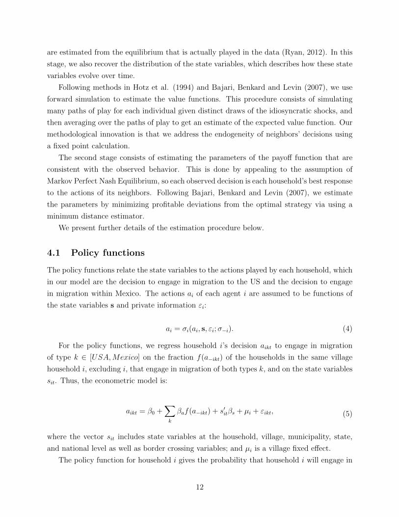
4.1 Policy functions

The policy functions relate the state variables to the actions played by each household, which

in our model are the decision to engage in migration to the US and the decision to engage

in migration within Mexico. The actions ai of each agent i are assumed to be functions of

the state variables s and private information εi:

ai = σi(ai, s, εi;σ−i). (4)

For the policy functions, we regress household i’s decision aikt to engage in migration

of type k ∈ [USA,Mexico] on the fraction f(a−ikt) of the households in the same village

household i, excluding i, that engage in migration of both types k, and on the state variables

sit. Thus, the econometric model is:

aikt = β0 +∑k

βaf(a−ikt) + s′itβs + µi + εikt, (5)

where the vector sit includes state variables at the household, village, municipality, state,

and national level as well as border crossing variables; and µi is a village fixed effect.

The policy function for household i gives the probability that household i will engage in

12

migration, conditional on the (publicly observable) state variables sit. Since policy functions

are based only on information that is observable to all households, household i’s policy

function also represents the beliefs that household i’s neighbors have about the probability

that household i will engage in migration.

The state variables in sit that we use for the policy functions include the number of

members in the household; the age of the household head; whether the first born is male; the

schooling of the household head; the average level of schooling, measured as the number of

years of education that have been completed, of household members 15 years old and above;

whether the household engaged in migration within Mexico the previous year; whether the

household engaged in migration to the US the previous year; the area of land owned by the

household that is irrigated for agricultural purposes, interacted with village precipitation;

the number of basic schools; the distance to the closest border crossing point; the crime rates

at the closest, second closest, and third closest border crossing points; the hourly wage in

the primary sector; and employment in the secondary sector.

Since the policy function for each player i depends on the policy functions for all other

players, we address the endogeneity of neighbors actions in the structural model by using a

fixed point algorithm in the forward simulation, as described below.

4.2 Transition densities

We estimate the distribution of next period’s state variables conditional on this period’s

state variables and actions using flexible transition densities. In particular, we use linear

regressions that relate the current level of the state variables to their lags, the lags of other

related state variables, and the lags of the action variables.

We model the following transition densities at the household level: the number of males

in the household, the number of males in the family,5 the household size, a dummy indicator

for whether the first born of the household was a male, household head schooling, household

average schooling, household maximum schooling, household land slope interacted with rain,

household land quality interacted with rain, and household irrigated land area interacted with

rain. We model these transition densities by regressing these variables on lagged values of

state and action variables. Thus, although we do not model schooling and other decisions

made by household (other than migration) explicitly, our models allows schooling and other

household-level variables to evolve endogenously conditional on state variables and actions

via the transition densities.

The age of the head of the household evolves deterministically, so next year’s age is

5We define a family as the household head, its spouse, and its children.

13

today’s age plus one.

At the village level, we regress the crime rate at the closest, second closest, and third

closest border crossing points on their lags and the lag of the primary sector wage.

At the municipality level, we regress the number of basic schools, the number of indige-

nous schools, and the number of students in the basic system on the lags of these same

variables, and the lags of the employment levels in the three sectors.

At the state level, we regress the employment shares in each sector on the lags of the

three shares, and on the lags of average wages.

At the national level, we regress average wages in the primary, secondary, and tertiary

sectors on the the lags of these three same variables.

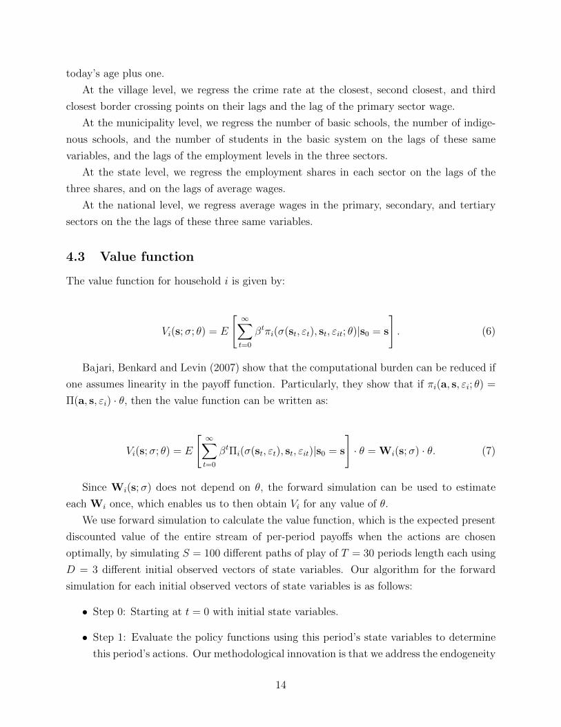
4.3 Value function

The value function for household i is given by:

Vi(s;σ; θ) = E

[∞∑t=0

βtπi(σ(st, εt), st, εit; θ)|s0 = s

]. (6)

Bajari, Benkard and Levin (2007) show that the computational burden can be reduced if

one assumes linearity in the payoff function. Particularly, they show that if πi(a, s, εi; θ) =

Π(a, s, εi) · θ, then the value function can be written as:

Vi(s;σ; θ) = E

[∞∑t=0

βtΠi(σ(st, εt), st, εit)|s0 = s

]· θ = Wi(s;σ) · θ. (7)

Since Wi(s;σ) does not depend on θ, the forward simulation can be used to estimate

each Wi once, which enables us to then obtain Vi for any value of θ.

We use forward simulation to calculate the value function, which is the expected present

discounted value of the entire stream of per-period payoffs when the actions are chosen

optimally, by simulating S = 100 different paths of play of T = 30 periods length each using

D = 3 different initial observed vectors of state variables. Our algorithm for the forward

simulation for each initial observed vectors of state variables is as follows:

• Step 0: Starting at t = 0 with initial state variables.

• Step 1: Evaluate the policy functions using this period’s state variables to determine

this period’s actions. Our methodological innovation is that we address the endogeneity

14

of neighbors’ decisions using a fixed point calculation, as described below.

• Step 2: Calculate this period’s payoffs as a function of this period’s state variables and

actions.

• Step 3: Evaluate the transition densities using this period’s state variables and action

variables to determine next period’s state variables.

• Repeat Steps 1-3 using next period’s state variables.

We sum the discounted payoffs over the T periods and average over the S simulations to

obtain the expected present discounted value of the entire stream of payoffs.

4.4 Fixed point algorithm

Our methodological innovation is that we address the endogeneity of neighbors’ decisions

using a fixed point calculation, as follows:

• Step 1: Estimate policy functions.

• Step 2: Use the observed fraction of neighbors with migration in the data as the initial

guess for the expected fraction of neighbors with migration in the policy function.

• Step 3: Predict the actions for all households using the policy function evaluated at

latest guess for the expected fraction of neighbors with migration.

• Step 4: Calculate the fraction of neighbors with migration using the predicted actions,

which becomes the new guess.

• Repeat Steps 3 and 4 until the difference between the guess and the predicted fraction

of neighbors with migration is below a certain threshold.

4.5 Estimating the structural parameters

We estimate the parameters θ by imposing the restriction that the observed equilibrium

is a Markov Perfect Nash Equilibrium. Then, the equilibrium condition Vi(s;σi, σ−i; θ) ≥Vi(s;σ

′i, σ−i; θ) yields a set of inequalities that are consistent with the assumed behavior. The

goal of the estimation procedure is to find the value of θ that makes all the inequalities to hold

at the same time. In practice, we will use an estimator that minimizes profitable deviations

from the optimal strategy. Bajari, Benkard and Levin (2007) prove the asymptotic properties

of this kind of estimator, which turns out to be consistent and asymptotically normal.

15

In order to estimate θ we compute alternative value functions Vi(s;σ′; θ) that result from

deviations from the policy function. We compute the corresponding actions that agents

would have taken and simulate a whole set of S paths of play of length T , with D initial

data sets. A deviation is profitable if the value of the discounted stream of payoffs under the

alternative strategy is greater than under the optimal policy. We estimate θ by finding the

θ that minimizes profitable deviations.

5 Data and Application to Rural Mexico

The economic importance of migration from Mexico to the US is twofold. Since the mid-

1980s, migration to the US has represented an employment opportunity for Mexicans during

a period of economic instability and increasing inequality in Mexico. In addition, it has

represented an important source of income via remittances, especially for rural households

(Esquivel and Huerta-Pineda, 2007).6 Remittances from the US to Mexico amount to 22.8

billion dollars per year, according to estimates from the World Bank (2012). According to

recent calculations, an average of 2,115 dollars in remittances is sent by each of the nearly

11 million Mexicans living in the US, which represents up to 2 percent of the Mexican GDP

(D’Vera et al., 2013). Some authors estimate that 13 percent of household total income and

16 percent of per capita income in Mexico come from migrant remittances (Taylor et al.,

2008).7

With a border 3200 kilometers long, the largest migration flow between two countries, and

a wage differential for low-skilled workers between the US and Mexico of 5 to 1 (Cornelious

and Salehya, 2007), the US-Mexico migration relationship also imposes challenges to policy-

makers of both countries. Beginning in 2000, Mexico moved away from its previous so-called

‘no policy policy’, and tried instead to pursue a more active policy to influence the US to

agree to a workers program and to increase the number of visas issued for Mexicans, although

its efforts got frustrated after the 9/11 attacks in September 2001. More recently, other

domestic policies have included the programs Paisano and Tres Por Uno, which facilitate the

temporary return during holidays of Mexicans legally living in the US and which match the

contributions of migrant clubs for the construction of facilities with social impact in Mexican

communities, respectively. On the US side, several reforms have been attempted to open

a path for legalization while also increasing expenditures to discourage illegal immigration,

6Esquivel and Huerta-Pineda (2007) find that 3 percent of urban households and up to 10 percent of ruralhouseholds in Mexico receive remittances.

7Castelhano et al. (2018) find that migrant remittances are not associated with increases in rural invest-ment in agricultural production in Mexico, however.

16

both of which affect mostly Mexicans. The most recent, the Deferred Action for Childhood

Arrivals, gives access to work permits to individuals who entered the country before they

were 16 years of age (Rojas Valdes, Lin Lawell and Taylor, 2018). On September 5, 2017,

the U.S. Department of Homeland Security initiated the phaseout of the Deferred Action for

Childhood Arrivals program (U.S. Department of Homeland Security, 2017).

We use data from the National Survey of Rural Households in Mexico (ENHRUM) in

its three rounds (2002, 2007, and 20108). The survey is a nationally representative sample

of Mexican rural households across 80 villages and includes information on the household

characteristics such as productive assets and production decisions. It also includes retrospec-

tive employment information: individuals report their job history back to 1980. With this

information, we construct an annual household-level panel data set that runs from 19909 to

2010, and that includes household composition variables such as household size, household

head age, and number of males in the household. For each individual, we have information

on whether they are working in the same village, in some other state within Mexico (internal

migration), or in the United States.

The survey also includes information about the plots of land owned by each household,

including slope (flat, inclined, or very inclined), quality (good, regular, or bad), irrigation

status, and land area.10 We construct variables for land slope and land quality for the

complete panel using the date at which each plot was acquired. Since a plot’s slope and

quality are unlikely to change over time (unless investments were taken to considerably

change the characteristics of the plots, which we do not observe very often in the data), we

interact the plot variables with a measure of contemporaneous precipitation at the village

level (Jessoe, Manning and Taylor, 2018) so that the resulting interaction variables vary

across households and over time. Rain data covers the period 1990 to 2007. The slope and

quality of household land interacted with contemporaneous precipitation captures shocks to

agricultural home production and therefore to household income that vary by household and

year and that may affect migration decisions.

We use information from the National Statistics Institute (INEGI) to control for the

urbanization and education infrastructure at the municipality level, including the number of

basic schools and the number of indigenous schools. We also include the number of registered

cars and buses. These data cover the period 1990 to 2010.

8The sample of 2010 is smaller than the sample of the two previous rounds because it was impossible toaccess some villages during that round due to violence and budget constraints.

9Since retrospective data from 1980 to 1989 included only some randomly selected individuals in eachvillage who reported their work history, we begin our panel data set in 1990.

10We use information on plots of land which are owned by the household because our data set does notinclude comparable information on plots of land that are rented or borrowed.

17

We also include aggregate variables that represent the broad state of the institutional and

economic environment relevant for migration. We use data from the INEGI on the fraction

of the labor force employed in each of the three productive sectors (primary, secondary,

and tertiary)11 at the state level, from 1995 to 2010. We use INEGI’s National Survey of

Employment and the methodology used in Campos-Vazquez, Hincapie and Rojas-Valdes

(2012) to calculate the hourly wage at the national level from 1990 to 2010 in each of the

three productive sectors and the average wage across all three sectors.

We use two sets of border crossing variables that measure the costs of migration. On

the Mexican side, we use INEGI’s data on crime to compute the homicide rate per 10,000

inhabitants at each of the 37 the Mexican border municipalities. On the United States’

side, we use data from the Border Patrol that include the number of border patrol agents,

apprehensions, and deaths of migrants at each of nine border sectors,12 and match each

border sector to its corresponding Mexican municipality.

We interact these border crossing variables (which are time-variant, but the same for all

villages at a given point in time) with measures of distance from the villages to the border

(which are time-invariant for each village, but vary for each village-border location pair).

We use a map from the International Boundary and Water Commission (2013) to obtain

the location of the 26 crossing-points from Mexico to the United States. Using the Google

Distance Matrix API, we obtain the shortest driving route from each of the 80 villages in

the sample to each of the 26 crossing-points, and match the corresponding municipality at

which these crossing-points are located. This procedure allows us to categorize the border

municipalities into those less than 1,000 kilometers from the village; and those between 1,000

and 2,000 kilometers from the village.

By interacting the distances to the border crossing points with the border crossing vari-

ables, we obtain the mean of each border crossing variable at each of the three closest crossing

points, and the mean of each border crossing variable within the municipalities that are in

each of the two distance categories defined above. We also compute the mean of each border

crossing variable among all the border municipalities.

Figure A.1 in Appendix A presents a map of the villages in our sample (denoted with a

filled black circle) and the US-Mexico border crossing points (denoted with a red X).

Table A.1 in Appendix A presents the summary statistics for the variables in our data

11The primary sector includes agriculture, livestock, forestry, hunting, and fisheries. The secondary sectorincludes the extraction industry and electricity, manufacturing, and construction. The tertiary sector includescommerce, restaurants and hotels, transportation, communication and storage, professional services, financialservices, corporate services, social services, and government and international organizations.

12A ’border sector’ is the term the Border Patrol uses to delineate regions along the border for theiradministrative purposes.

18

set. Table A.2 in Appendix A presents the within and between variation for the migration

variables. ’Within’ variation is the variation in the migration variable across years for a

given village. ’Between’ variation is the variation in the migration variable across villages

for a given year.

6 Results

6.1 Policy functions and transition densities

In Table A.3 in Appendix A, we present the results of the policy functions relating states

to actions. Column (1) presents the policy function for migration to the US. Column (2)

presents the policy function for migration within Mexico. The implications of these results

are discussed in detail in Rojas Valdes, Lin Lawell and Taylor (2018). We use the coefficients

that are significant at a 10% level in our structural model to predict the actions played given

the state variables. To address the endogeneity of neighbors’ decisions, we use a fixed point

calculation.

The policy functions we estimate represent the empirical relationship between the actions

and states observed in the data. Without imposing any structure, these policy functions

simply characterize what households do mechanically as a function of the state vector. As

the policy functions are reduced-form regressions correlating actions to states, their results

therefore show correlations, not causation.

Our estimated policy functions in Table A.3 in Appendix A show a significant negative

own-migration strategic interaction: a household’s probability of engaging in migration to

the US is negatively correlated with the fraction of neighbors who engage in migration to

the US, and a household’s probability of engaging in migration within Mexico is negatively

correlated with the fraction of neighbors who engage in migration within Mexico. Risk

sharing considerations, competition effects (Rojas Valdes, Lin Lawell and Taylor, 2018),

and a limited number of employers at the destination site who do not discriminate against

migrants from elsewhere (Carrington, Detragiache and Vishwanath, 1996) may be possible

explanations for the negative own-migration strategic interaction.

Our policy functions show a significant positive other-migration strategic interaction: a

household’s probability of engaging in migration to the US is positively correlated with the

fraction of neighbors who engage in migration within Mexico, and a household’s probability

of engaging in migration within Mexico is positively correlated with the fraction of neighbors

who engage in migration to the US. One possible explanation for the positive other-migration

strategic interaction it that it results from the negative own-migration strategic interaction:

19

if a household is less likely to engage in migration to a destination to which its neighbors are

engaging in migration, then it may engage in migration elsewhere instead.

Our policy functions also show that there is persistence in the decision to engage in

migration to the US or within Mexico: there is a significant positive correlation between

lagged migration to the US and the probability of migration to the US, and similarly a

significant positive correlation between lagged migration within Mexico and the probability

of migration within Mexico.

In Tables A.4-A.6 in Appendix A, we present the results of the transition densities for the

variables at the household, municipality, state, and national levels. These transition densities

describe the behavior of state variables over time. We regress the level of each variable on

the lag of other relevant state variables. We use the coefficients that are significant at a 10%

level to predict the value of next period’s state variables, which affect the actions taken of

each household in next period as well as the payoff functions.

6.2 Structural parameters

We present the parameter estimates of our structural model in Table 1. The parameters we

estimate are the coefficients in the per-period payoff function πi(a, s, εi; θ).

According to our results, the coefficient in the per-period payoff on household head school-

ing is significant and positive, which indicates that the higher the household head schooling,

the higher the per-period payoff to the household.

The coefficient on household land quality interacted with rain is significant and negative.

Since higher values of our index for household land quality denote a lower land quality,

the significant negative coefficient on the interaction indicates that the higher quality the

household land and the more rain, the higher the per-period payoff to the household.

The significant negative coefficient on household land quality interacted with rain inter-

acted with migration to the US indicates that the higher quality the household land and

the more rain, the higher the per-period payoff to having a household member migrate to

the US. This result suggests that home agricultural production and migration to the US are

complements. The likely mechanism is as follows. Higher incomes from home agricultural

production relax household credit constraints and enable the household to send a member to

migrate to the US. Migration to the US, in turn, generates additional income for the house-

hold via remittances, which enables the household to further improve their home agricultural

production.

The significant positive coefficient on household land quality interacted with rain inter-

acted with migration within Mexico indicates that the higher quality the household land and

20

the more rain, the lower the per-period payoff on net to having a household member migrate

within Mexico. This result suggests that home agricultural production and migration within

Mexico are substitutes. Unlike migration to the US, which is costly but also generates in-

come for the household via remittances, migration within Mexico is a substitute rather than

a complement to home agricultural production, possibly at least in part because it is less

costly and also generates little if any income for the household via remittances.

As indicated by the significant positive coefficient on hourly wage, the higher the hourly

wage, the higher the per-period payoff to the household. The significant positive coefficient

on hourly wage interacted with migration to the US indicates that the higher the hourly

wage, the higher the per-period payoff to having a household member migrate to the US. In

contrast, the significant negative coefficient on hourly wage interacted with migration within

Mexico, which is smaller in magnitude than the significant positive coefficient on hourly

wage, indicates that the hourly wage has less of a positive effect on net on the per-period

payoff when a household engages in migration within Mexico.

The significant positive coefficients on the variables interacting crime rate with migration

to the US indicates that the higher the crime rate in Mexico, the higher the per-period payoff

to having a household member migrate to the US. In contrast, the effects of crime rates at

the border on the payoff to having a household member migrate within Mexico are mixed.

6.3 Comparing structural model with observed data

As seen in Table A.7 in Appendix A, which compares welfare calculated using observed data

with the welfare predicted by our structural econometric model, our structural econometric

model does a fairly good job of predicting welfare calculated based on observed data.

Similarly, when comparing the migration observed in the data in Tables A.8 and A.9 in

Appendix A with the analogous migration statistics predicted by our structural econometric

model in Tables A.10 and A.11 in Appendix A, our structural econometric model does a

fairly good job of predicting the levels and upward trends in migration observed in the data.

7 Counterfactual simulations

We use the estimated parameters to simulate the effects of counterfactual policy scenarios,

including those regarding wages, government policy, schooling, crime rates at the border,

and precipitation, on migration decisions and welfare. In order to disentangle the effects of

strategic interactions and dynamic behavior in our model, we also simulate counterfactual

scenarios in which remove strategic interactions, and counterfactual scenarios in which we

21

remove dynamic behavior.

For each counterfactual scenario, we simulate the effects of a counterfactual change that

takes place in the year 1997 on migration and welfare over the years 1997 to 2007. We

then compare the average welfare per household-year and the fraction of households with

migration under that counterfactual scenario with those under the base case of no change

using two-sample t-tests.

There are several channels through which each counterfactual change may affect house-

hold welfare. First, the counterfactual change (e.g., in wages) may affect household welfare

directly. Second, the counterfactual change may affect migration decisions which affect

household welfare. Third, the counterfactual change may affect other decisions of the house-

hold which may affect household welfare. Although we focus on explicitly modeling the

migration decisions of the households, our model implicitly captures schooling and other

decisions made by household by allowing schooling and other household-level variables to

evolve endogenously conditional on state variables and actions via the transition densities.

Fourth, changes in actions and/or state variables resulting from the counterfactual change

may affect future values of the state variables, which may affect future actions and/or wel-

fare. Our estimates of the changes in welfare that arise in each counterfactual simulation

capture all channels through which the counterfactual scenario may affect household welfare.

7.1 Wages

Real wages in Mexico plunged after the 1994 crisis and recovered slowly during the period

covered by our data set. We simulate changes in the hourly wage in the primary sector.

The primary sector includes agriculture, livestock, forestry, hunting, and fisheries. In our

structural econometric model, the hourly wage in the primary sector affects both the policy

functions and the transition densities.

In 2010, 1 US dollar bought 12.80 Mexican pesos. Thus, the mean hourly wage in

the primary sector in our data set, as reported in the summary statistics in Table A.1 in

Appendix A, of 29 pesos per hour in 2010 pesos is roughly equivalent to 2.3 dollars per hour

in 2010 US dollars. Our simulated changes in the primary sector wage ranging from a 50%

decrease to a 50% increase therefore represent simulated primary sector wages ranging from

a mean of 14.5 pesos (approximately 1.15 US dollars) per hour after a 50% decrease, to a

mean of 43.5 pesos (approximately 3.45 US dollars) per hour after a 50% increase. Even

after a 50% increase in primary sector wage, the largest increase in primary sector wage that

we simulate, mean wages are still less than half the 1997 US federal minimum wage of 7.01

22

dollars in 2010 US dollars.13

Figure 1 presents the percentage change from the base case in the fraction of households

with migration to the US and within Mexico over the entire simulation period (1997-2007)

under each simulated change in primary sector wages in the initial year of the simulation

(1997). Error bars indicate the 90% confidence interval from a two-sample t-test comparing

the results under the counterfactual simulation with those under the base case of no change.

Results show that an increase in primary sector wages leads to a statistically significant

increase in migration to the US and within Mexico. Similarly, a decrease in primary sector

wages leads to statistically significant decreases in migration to both the US and within

Mexico in all but one of the simulated scenarios (that of a 15% decrease). Moreover, the

more dramatic the simulated change, the more dramatic the response of the fraction of

households with migration. In addition, in all the cases the where changes in migration are

statistically significant, the magnitudes of the changes in the fraction of households with

migration to the US are much larger than those of the changes in the fraction of households

with migration within Mexico.

Figure 2 presents the percentage change from the base case in the average welfare per

household-year over the entire simulation period (1997-2007) under each simulated change

in primary sector wages in the initial year of the simulation (1997). Error bars indicate

the 90% confidence interval from a two-sample t-test. As expected, a decrease in primary

sector wages leads to a statistically significant decrease in average welfare per household-

year, while an increase in primary sector wages leads to a statistically significant increase in

average welfare per household-year.

In addition to the pooled results, we also analyze the results by village. In Figure 3

we show the changes by village in the fraction of households with migration to the US and

within Mexico over the entire simulation period (1997-2007) under a 10% decrease and a 10%

increase in primary sector wages, respectively, in the initial year of the simulation (1997).

The red dots denote villages that experience a statistically significant decrease in the fraction

of households with migration; the green dots denote villages that experience a statistically

significant increase in the fraction of households with migration; and the black dots denote

villages with no statistically significant change. We find that there is some heterogeneity at

the village level in the changes in the fraction of households with migration to the US and

within Mexico.

To examine how this heterogeneity relates to observable village characteristics, we analyze

the determinants of significant changes at the village level in the fraction of households with

13The US federal minimum wage in 1997 was 5.15 dollars in 1997 dollars (US Department of Labor, 2017),which is equivalent to 7.01 dollars in 2010 US dollars.

23

migration. To do so, we regress the village-level changes in the fraction of households with

migration over the entire simulation period (1997-2007) that are significant at a 10% level

under a simulated 10% increase and a simulated 10% decrease in primary sector wages in the

initial year of the simulation (1997), respectively, on the initial village, municipality, state,

and national characteristics from the initial year of the simulation (1997). Table 2 presents

the results.

As seen in Table 2, under a 10% increase in primary sector wages, significant changes

in migration to the US are positively correlated with the initial fraction of households with

migration within Mexico. This suggests that when wages increase, greater increases in

migration to the US are more likely to occur in villages that were already mobile, as measured

by the initial fraction of households with migration within Mexico.

Also as seen in Table 2, significant changes in migration within Mexico are positively

correlated with the initial number of males in the household, and negatively correlated with

the initial household size, which suggests that when wages increase, greater increases in

migration within Mexico are more likely to occur where there is a larger share of males in

the household who can take advantage of those increases in wages. Significant changes in

migration within Mexico are also positively correlated with the distance to the US border

and the initial household head age.

Under a 10% decrease in wages in the primary sector, Table 2 shows that significant

changes in migration to the US are negatively correlated with the initial household head

schooling, which suggests that when the wage decreases, larger decreases in migration to

the US are more likely to occur in villages where the household head is more educated,

perhaps because a more educated household head increases the return from having other

household members stay at home, therefore reducing migration to the US, especially when

the household is more credit-constrained. In contrast, significant changes in migration to the

US are positively correlated with the initial household average schooling, which suggests that

when the wage decreases, larger increases in migration to the US are more likely to occur

in villages where the household average schooling is higher, perhaps because more educated

households have higher returns to migration to the US, and thus are more likely to engage

in migration to the US when credit-constrained.

In Figure 4, we present the changes in average welfare per household-year at the village

level under simulated changes of a 10% decrease and a 10% increase in primary sector wages,

respectively. Consistent with the aggregate results, most of the villages experience a decrease

in welfare under a 10% decrease in primary sector wages, while all of the villages except for

one experience a statistically significant increase in welfare under a 10% increase in primary

24

sector wages.14

Thus, our simulations regarding wages paid in the primary sector show that migration to

US and within Mexico increase with primary sector wage in the pooled results, but there is

some heterogeneity across villages. Average welfare per household-year is increasing in the

primary sector wage for almost all villages.

7.2 Migration policy

Given the significance of migration policy, especially from the US perspective, an important

question is: what is the effect of migration policies on migration and welfare? We simulate

two types of policies: a floor on schooling for migration to the US, and a cap on the number

of households with migration to the US.

7.2.1 Minimum schooling requirement for migration to the US

The first migration policy we simulate is a minimum schooling requirement that specifies

a minimum threshold household average schooling needed in order for a household to be

allowed to engage in migration to US in 1997, the first year of the simulation. We set the

threshold to range from 50% to 150% of the average household schooling observed in the

data.

As seen in Figure 5, a minimum schooling requirement for migration to the US would have

direct negative effects on migration to the US. The greater the requirement for minimum

schooling for migration to the US, the more dramatic the drop in migration to the US, with

all the simulated changes being statistically significant. Moreover, a minimum schooling

requirement for migration to the US would lead to changes in migration within Mexico as

well: a minimum schooling requirement for migration to the US from a 25% of the average

schooling up to a 150% of the average schooling leads to a statistically significant decrease

14Although there is less heterogeneity among villages in the sign of the welfare effects, especially under a10% increase in primary sector wages, we examine how the sign and magnitudes of the village-level welfareresults relate to observable village characteristics by analyzing the determinants of significant changes atthe village level in average welfare per household-year. To do so, we regress the village-level changes inthe average welfare per household-year over the entire simulation period (1997-2007) that are significantat a 10% level under a simulated 10% increase and a simulated 10% decrease in primary sector wages inthe initial year of the simulation (1997), respectively, on the initial village, municipality, state, and nationalcharacteristics from the initial year of the simulation (1997). As seen in Table B.1 in Appendix B, statisticallysignificant changes in welfare under a 10% increase in wages in the primary sector are positively correlatedwith the initial fraction of households with migration within Mexico and the initial household head age, whilestatistically significant changes in welfare under a 10% decrease in welfare are positively correlated with theinitial number of males in the household and the initial household head age, and negatively correlatedwith the initial fraction of households with migration to the US and the initial fraction of households withmigration within Mexico.

25

in the fraction of households with migration within Mexico. Figure 6 shows that this policy

leads to a statistically significant decrease in average welfare per household-year in every

simulated minimum threshold of schooling required for migration.

As seen in Figure B.1 in Appendix B, a minimum schooling requirement for migration

to the US would have a negative effect on the fraction of households with migration to the

US in almost every village, and a significant negative effect on the fraction of households

with migration within Mexico in some villages.15 As seen in Figure B.2 in Appendix B, most

of the villages experience a statistically significant decrease in welfare under the simulated

minimum thresholds of schooling for migration to the US.16

7.2.2 Cap on total migration to the US

The second migration policy we simulate is a cap on total migration to the US. For this

counterfactual policy, we set a cap that denies migration to US to a certain percentage,

ranging from 50% to 90%, of the total number of households who would have engaged in

migration to the US under the base case simulation. That is, of the households who engage

in migration to the US under the base case, we restrict a randomly chosen 50% and 90% of

these households from migrating to the US in 1997, the first year of the simulation.

As seen in Figure 7, the simulated caps have statistically significant negative effects on

migration not only to the US but also within Mexico. Moreover, the size of the reduction in

the fraction of households with migration to the US is greater than the cap. For example, a

cap that denies US migration to 50% of the households that would have engaged in migration

to the US in the base case leads to a decrease in the fraction of households with migration to

the US of 70% for the period of our simulations, due to the spillover effects of the migration

decisions. As seen in Figure 8, all our simulated caps on migration lead to a statistically

significant decrease in welfare.

In Figure B.3 in Appendix B, we present the effects of a cap of 90% of base case US mi-

15In Table B.2 in Appendix B we show that, under a simulated threshold of 110% of the average schoolingfor migration, significant changes in the fraction of households with migration to the US are positivelycorrelated with the initial household head schooling at the village level, and negatively correlated with theinitial household size and the initial fraction of households with migration to the US, whereas significantchanges in migration within Mexico are positively correlated with initial household land quality. Similarly,under a simulated threshold of 90% of the average schooling, the shares of employment in the primary andsecondary sectors are associated with significant decreases in migration both to the US and within Mexico,and the initial fraction of households with migration to the US is correlated with significant decreasesmigration to the US.

16As shown in Table B.3 in Appendix B, significant changes in welfare under a threshold of 110% and90% of average schooling are positively correlated with the initial household head schooling and the initialfraction of households with migration to the US; in addition, significant changes in welfare under a simulatedthreshold of 90% of average schooling are also negatively correlated with the initial shares of employment inthe primary and secondary sectors.

26

gration on migration by village. Consistent with our aggregate results, all villages experience

a statistically significant decrease in migration to the US, while some villages experience a

statistically significant decrease in migration within Mexico.17 Figure B.4 in Appendix B

shows that all the villages experience a statistically significant decrease in welfare under the

simulated cap of migration.18

Strategic interactions explain why policies that decrease migration to the US also de-

crease migration within Mexico. Owing to the significant positive other-migration strategic

interaction in the policy functions in Table A.3 in Appendix A, decreases in migration to US

by neighbors are associated with a decrease in a household’s probability of migrating within

Mexico.

Dynamic behavior explains why a cap on total migration to the US causes migration to

the US to decrease by more than what is required by the policy. Owing to the significant

positive effect of lagged migration to the US on the probability of migration to the US in the

policy functions in Table A.3 in Appendix A, there is persistence in the decision to engage

in migration to the US. Thus, policies that restrict migration to the US are amplified over

time.

We further analyze the effects of strategic interactions and dynamic behavior in our

counterfactual scenarios below that remove strategic interactions and dynamic behavior,

respectively.

7.3 Schooling

Policies to improve the levels of schooling assume that a higher level of human capital will

improve earning opportunities. We simulate the effect of changes in each the three schooling

variables in our model in turn: the schooling of the household head, the average schooling

of the household, and the maximum schooling of the household.

17Table B.4 in Appendix B shows that under a simulated cap denying migration to 90% of the householdsthat would have engaged in migration to the US in the base case, significant changes in the fraction ofhouseholds with migration to the US are positively correlated with initial household head schooling andthe initial fraction of households with migration within Mexico, and negatively correlated with the initialhousehold size and the initial fraction of households with migration to the US. Under this simulation,significant changes in migration within Mexico are negatively correlated with the initial fraction of householdswith migration within Mexico.

18As seen in Table B.5 in Appendix B, significant changes in welfare are positively correlated with the initialhousehold head schooling, and negatively correlated with the initial fraction of households with migrationto the US and the initial household land quality.

27

7.3.1 Household head schooling

Household head schooling affects both the policy functions and the transition densities. As

seen in Figure B.5 in Appendix B, counterfactual increases in household head schooling

have a negative effect on the fraction of households with migration to the US and within

Mexico, and the effect is significant for the very dramatic changes of an increase of 50%

for the case of migration to the US, and for increases of 25% and 50% in household head

schooling for the case of migration within Mexico. Almost symmetrically, a very dramatic

decrease of 50% in the household head schooling leads to a statistically significant increase

in migration to the US, whereas every simulated decrease in household head schooling leads

to a statistically significant increase in migration within Mexico. Moreover, the lower the

household head schooling, the higher the migration to the US and within Mexico, with the

changes in migration within Mexico being larger in magnitude. Figure B.6 in Appendix

B shows that all the simulated increases in household head schooling lead to statistically

significant increases in welfare, whereas most of the simulated decreases in household head

schooling lead to statistically significant decreases in welfare.

Figure B.7 in Appendix B shows the changes in the fraction of households with migration

by village under a 10% increase or decrease in household head schooling. We see that

the results are heterogeneous by village.19 As seen in Figure B.8 in Appendix B, there is

heterogeneity at the village level in the changes in average welfare per household-year under

a 10% decrease in household head schooling, but most villages experience a statistically

significant increase in average welfare per household-year under a 10% increase in household

head schooling.20

7.3.2 Average household schooling

Average household schooling affects both the policy functions and the transition densities.

According to the results of our counterfactual simulations of changes in average household

schooling, we find in Figure B.9 in Appendix B that there are statistically significant effects

on migration to the US under very dramatic increases or decreases in average schooling.

19Table B.6 in Appendix B shows that significant changes in the fraction of households with migrationwithin Mexico under a 10% increase in household head schooling are positively correlated with the distanceto the nearest border crossing point and the initial household head age. Significant changes in migration tothe US are positively correlated with the initial fraction of households with migration within Mexico undera 10% increase in household head schooling, and negatively correlated with the intial number of householdmembers under a 10% decrease in household head schooling.

20Table B.7 in Appendix B shows that statistically significant changes in welfare are positively correlatedwith the initial fraction of households with migration within Mexico under a 10% decrease in household headschooling.

28

For migration within Mexico, increases of 15%, 25%, and 50% in average schooling have

a statistically significant and positive effect on migration within Mexico; and decreases of

15%, 25%, and 50% have a statistically significant and negative effect on migration within

Mexico. As seen in Figure B.10 in Appendix B, every simulated increase in household average

schooling leads to a statistically significant decreases in average welfare per household-year,

and every simulated decrease in household average schooling leads to a statistically significant

increase in average welfare per household-year.

As seen in Figure B.11 in Appendix B, the effects of changes in average household school-

ing on migration vary by village.21 As seen in Figure B.12 in Appendix B, the effects of

changes in average household schooling on welfare vary by village as well.22

7.3.3 Maximum household schooling

Maximum household schooling affects the transition densities. For our counterfactual sim-

ulations of changes in maximum household schooling, and similar to our findings in the

simulations of changes in the household average schooling, we find in Figure B.13 in Ap-

pendix B that dramatic increases in the maximum schooling leads to statistically significant

increases in migration within Mexico, while dramatic decreases in the maximum schooling

leads to statistically significant decreases in the fraction of households with migration within

Mexico. As seen in Figure B.14 in Appendix B, every simulated decrease in household

maximum schooling leads to a statistically significant increase in welfare, while only dra-

matic simulated increases in maximum schooling lead to statistically significant decreases in

welfare.

As seen in Figure B.15 in Appendix B, there is heterogeneity at the village level in

the effects of changes in the household average schooling on migration.23 Similar to the

21As seen in Table B.8 in Appendix B, significant changes in migration to the US are positively correlatedwith the initial fraction of households with migration within Mexico under a 10% increase in the householdaverage schooling, and with initial employment in the secondary sector under a 10% decrease in the house-hold average schooling. Significant changes in migration within Mexico is negatively correlated with initialhousehold size and positively correlated with the initial fraction of households with migration to the USunder a 10% increase in the household average schooling.

22Significant changes in average welfare per household year under a 10% increase in household averageschooling are positively correlated with the initial employment share in the primary and secondary sectors,and with the initial fraction of households with migration within Mexico, as seen in Table B.9 in AppendixB.

23As shown in Table B.10 in Appendix B, significant changes in migration to the US are negatively corre-lated with initial employment in the primary sector under a 10% increase in maximum household schooling,and positively correlated with the initial fraction of households with migration within Mexico under a 10%decrease in maximum household schooling. Significant changes in migration within Mexico are negativelycorrelated with initial household head schooling and the initial fraction of households with migration withinMexico and positively correlated with initial household average schooling under a 10% increase in maximumhousehold schooling; positively correlated with initial employment in the secondary sector under a 10% de-

29

aggregate results, we find that most of the villages experience an increase in welfare under

a simulated decrease in maximum schooling of 10%, and that there is some heterogeneity

under a simulated increase of 10% in maximum schooling, as seen in Figure B.16 in Appendix

B.24

7.3.4 Mechanisms

To summarize the results of our counterfactual simulations of schooling, we find that as

household head schooling increases, migration to US and within Mexico decrease, while

average welfare per household-year increases. In contrast, as household average schooling or

household maximum schooling increases, migration to US and within Mexico increase, while

average welfare per household-year decreases.

One possible explanation is that households with higher levels of household average

schooling or household maximum schooling have better returns to education outside the

village that they are willing to take advantage of by sending a member to migrate. In con-

trast, a more educated household head increases the return for other household members to

stay at home, therefore reducing migration both to the US and within Mexico.

The effects of schooling on migration decisions arise through the policy functions in Table

A.3 in Appendix A. From the policy functions, migration to US and within Mexico decrease

with household head schooling, but increase with household average schooling or household

maximum schooling.

As seen in our parameter estimates in Table 1, schooling affects per-period payoffs (and

therefore welfare) regardless of the migration decision. Thus, the welfare results arise from

the direct effect of schooling on household per-payoffs. Average welfare per household-year

increases with household head schooling and decreases with household average schooling or

household maximum schooling, regardless of the migration decision.

7.4 Crime rates at the border

Crime rates in Mexico experienced a dramatic increase after 2006. An important question

that therefore arises is: what is the effect of crime rates at the border on migration decisions?

We simulate changes in the crime rate at the three closest border crossing points from the

household villages. Changes in crime rate affect both the policy functions and the transition

densities in our structural econometric model.

crease in maximum household schooling; and positively correlated with initial employment in the primarysector under both a 10% increase and a 10% decrease in maximum household schooling.

24Statistically significant changes in welfare at the village level are positively correlated with initial house-hold land quality, as seen in Table B.11 in Appendix B.

30

Figure B.17 reports no statistically significant change in migration to the US and within

Mexico under any of the simulated scenarios of changes in crime rate at the border in the

pooled results. Similarly, as seen in Figure B.18 in Appendix B, we find that, except under

a dramatic increase of 50% in crime rate at the border, there are no statistically significant

changes in the average welfare per household-year in the pooled results.

As seen in Figure B.19 in Appendix B, there is some heterogeneity in the changes in

the fraction of households with migration to the US and within Mexico at the village level.

As seen in Table B.12 in Appendix B, under a 10% increase in crime rates at the border,

significant changes in migration to the US are positively correlated with the initial fraction

of households with migration within Mexico, whereas significant changes in the fraction of

households with migration within Mexico are negatively correlated with the initial employ-

ment share in the secondary sector and the initial fraction of the households with migration

within Mexico, and positively correlated with initial household land quality. Under a sim-

ulated 10% decrease in crime rates at the border, significant changes in migration to the

US are negatively correlated with the initial number of males in the household, whereas

significant changes in migration within Mexico are negatively correlated with the initial em-

ployment share in the secondary sector and positively correlated with the initial fraction of

households with migration to the US.

While in the aggregate results there are no statistically significant changes in welfare,

there is some heterogeneity at the village level in the changes on average welfare per household-

year, as can be seen in Figure B.20 in Appendix B, and the determinants of which are pre-

sented in Table B.13 in Appendix B. Under a simulated 10% increase in crime rates at the

border, households with better initial land quality experience increases in migration within

Mexico as well as increases in average welfare per household-year.

7.5 Precipitation

Changes in climatic conditions are important determinants of productivity in agriculture and

may have implications for migration. We simulate changes in precipitation, which may affect

different households differently depending on the soil quality on their land. In our structural

econometric model, precipitation has a significant effect on the transition densities.

As seen in Figure B.21 in Appendix B, we find that a 10% decrease in precipitation

leads to a statistically significant increase in migration to the US.25 We find in Figure B.23

25As seen in Figure B.22 in Appendix B, there is heterogeneity by village in the effects of a 10% increaseand a 10% decrease in precipitation on the fraction of households with migration to the US and withinMexico. As shown in Table B.14 in Appendix B, significant changes in migration to the US are positivelycorrelated with initial household average schooling under a 10% increase in precipitation. Significant changes

31

in Appendix B that this decrease of 10% in precipitation leads to a statistically significant

increase in average welfare per household-year.26

Our finding that decreases in precipitation may increase migration to the US is consistent

with previous studies that show that other adverse weather conditions, including extreme

heat (Jessoe, Manning and Taylor, 2018) and hurricanes (Mahajan and Yang, 2017), increase

migration within Mexico (from rural to urban areas) and to the US.

7.6 Removing strategic interactions

In our structural econometric model, strategic interactions can arise through several channels.

First, strategic interactions can arise in the policy functions if neighbors’ actions affect a

household’s strategy. Second, strategic interactions can arise in the transition densities if

the actions of households in the village affect future values of the the state variables faced

by a household. Third, strategic interactions can affect the per-period payoff of a household.

In order to disentangle the effects of strategic interactions in our model, we simulate

counterfactual scenarios in which we remove strategic interactions. For these counterfactual

scenarios, we set the coefficients on the fraction of neighbors with migration to the US and

within Mexico to be 0 in the policy functions; we set the coefficients on the lagged fraction of

households with migration to the US and within Mexico to be 0 in the transition densities;

and we set the coefficients on all terms involving the fraction of neighbors with migration to

be 0 in the per-period payoff function. All other coefficients and parameter values remain

the same.

The results from our counterfactual scenario eliminating strategic interactions are pre-

sented in Table 3. We find that the fraction of household with migrants to both the US and

within Mexico would be considerably higher if there were no strategic interactions. When

we look at the heterogeneity of these changes at the village level in Figure B.25 in Appendix

B, we observe that these increases in migration would occur in most of the villages in our

sample.

Also in Table 3 we show that in the absence of strategic interactions, the average welfare

per household-year would be lower than in the base case scenario. As seen in Figure B.26 in

in migration within Mexico are positively correlated with the initial number of males in the household and theinitial fraction of households with migration to the US, but negatively correlated with the initial employmentin the secondary sector.

26As seen in Figure B.24 in Appendix B, there is heterogeneity by village in the effects of a 10% increaseand a 10% decrease in precipitation on average welfare per household-year. As shown in Table B.15 inAppendix B, significant changes in average welfare per household-year under a 10% decrease in precipitationare positively correlated with the distance to the closest border crossing point, initial employment in theprimary and secondary sectors, and initial household head age.

32

Appendix B, average welfare per household-year would decrease in all villages in our sample.

Thus, strategic interactions are welfare-increasing.

The results from our counterfactual simulations of migration policy above show that a

cap on migration to the US decreases welfare and also decreases migration to both the US

and within Mexico. To better understand the role of strategic interactions when there is a

cap on migration to the US, we simulate the same caps on migration from a 50% up to a

90% of the migration in the base case, but without allowing for strategic interactions.

In Figure 9 we present the results of the cap of migration with no strategic interactions.

Migration to the US still decreases considerably and by more than what the cap was intended

to reduce over our simulation period. But now, migration within Mexico increases, in contrast

to the situation where strategic interactions took place. Figure B.30 in Appendix B shows

that migration to the US decreases in all the villages in our sample, while there are some

villages with no change in migration within Mexico. Strategic interactions therefore explain

why policies that decrease migration to the US also decrease migration within Mexico.

In Figure B.29 we show that the decrease in welfare resulting from a migration cap is

even greater in the absence of strategic interactions. As seen in Figure B.31 in Appendix

B, average welfare per household-year would decrease in all villages in our sample. The

absence of strategic interactions leads to a more inefficient scenario, with more migration

within Mexico, and with a larger loss in welfare resulting from the cap on migration to the

US.

7.7 Removing dynamic behavior

In order to disentangle the effects of dynamic behavior in our model, we simulate counter-

factual scenarios in which we remove dynamic behavior. For these counterfactual scenarios,

we set the discount factor β to 0, and we set the coefficients on lagged migration to US and

within Mexico to 0 in both the US migration and Mexico migration policy functions. All

other coefficients and parameter values remain the same.

The results from our counterfactual scenarios eliminating dynamic behavior are presented

in Table 4. When households do not consider the future when making their decisions, both

migration to the US and within Mexico decrease, and average welfare per household-year

decreases as well. This aggregate result is also reflected in the pattern at the village level,

as observed in Figures B.27 and B.28 in Appendix B. As seen in Figure B.28 in Appendix

B, average welfare per household-year would decrease in all villages in our sample. Thus,

household welfare is higher when households behave dynamically and consider the future

when making decisions in the present.

33

The results from our counterfactual simulations of migration policy above show that a

cap on migration to the US decreases welfare and also decreases migration to both the US

and within Mexico. To better understand the role of dynamic behavior when there is a cap

on migration to the US, we simulate the same caps on migration from a 50% up to a 90% of

the migration in the base case, but without allowing for dynamic behavior.

In Figure 10, we show the effects of a cap on migration to the US on migration in the

absence of dynamic behavior. Migration to the US decreases even more under a cap on

migration in the absence of dynamic behavior, while migration within Mexico decreases

considerably as well. The decrease in welfare resulting from a migration cap is more than 2

orders of magnitude greater in the absence of dynamic behavior, as shown in Figure B.32. As

seen in Figure B.34 in Appendix B, average welfare per household-year would decrease in all

villages in our sample. Thus, in the absence of dynamic behavior, the decrease in migration

to the US and within Mexico and the reduction in welfare as a result of a migration cap

would be even more severe.

8 Discussion and Conclusion

Dynamic behavior and strategic interactions are important features of migration decisions.

Analyses that ignore the possibility of strategic interactions or dynamic behavior lead to

misleading results. We build on the previous literature on the determinants of migration by

estimating a structural econometric model that incorporates dynamic behavior and strategic

interactions, and that enables us to calculate welfare and to analyze the effects of counter-

factual scenarios on decisions and welfare.

We use the estimated parameters to simulate the effects of counterfactual policy scenarios,

including those regarding wages, government policy, schooling, crime rates at the border,

and precipitation, on migration decisions and welfare. In order to disentangle the effects of

strategic interactions and dynamic behavior in our model, we also simulate counterfactual

scenarios in which remove strategic interactions, and counterfactual scenarios in which we

remove dynamic behavior.

Our counterfactual simulations regarding wages paid in the primary sector show that

migration to US and within Mexico increase with primary sector wage in the pooled results,

but there is some heterogeneity across villages. Average welfare per household-year is in-

creasing in the primary sector wage for almost all villages. Increases in wages in Mexico may

increase migration within Mexico if households send a member to migrate within Mexico

to take advantage of the higher wage. Increases in wages and income also enable poor and

credit-constrained households to better afford investment in schooling, increasing their future

34

expected wage and making future migration more affordable to poor and credit-constrained

households.

We find that increases in the wage in Mexico not only increase migration within Mexico,

but also increase migration to the US, likely because higher wages make migration to the

US becomes more affordable to poor and credit-constrained households. These results are

comparable to those of other studies that find that financial constraints are an important

determinant of migration and migration selectivity. For example, Angelucci (2015) finds that

Oportunidades, the flagship conditional cash transfer program of Mexico, increases migration

from Mexico to the US, which similarly provides evidence that poor households in Mexico

face binding financial constraints.

Furthermore, our results show that changes in wages have heterogeneous effects by village:

when the local wage increases, there is more migration within Mexico in villages with smaller

households, with more males, and older household heads; while there is more migration to

the US in villages that already have migrants within Mexico. On the other hand, when wages

decrease, there is more migration to the US from villages with poorly educated household

heads but with a higher average household schooling, consistent with evidence that changes

in income relax credit constraints on poor and low educated households but not on the

poorest and least educated.

Our result that increases in wages in Mexico will increase migration to the US contradicts

a common belief that improving the income of poor households would reduce migration, and

therefore that, in order to keep Mexicans in Mexico, one simply needs to improve economic

opportunities for Mexicans in their home country. Thus, since it is usually assumed that

labor moves to the United States mainly because of a lack of opportunities in Mexico (in

other words, implying some substitution across activities), our results finding evidence to

the contrary have important implications for the discussion and design of policy.

In terms of counterfactual government migration policy, we find that a minimum thresh-

old household average schooling needed for migration to US decreases migration not only to

the US but also within Mexico, and also decreases average welfare per household-year. A

cap on total migration to the US decreases migration not only to the US but also within

Mexico as well, causes migration to the US to decrease by more than what is required by

the policy, and decreases average welfare per household-year.

The current policy discussion on border enforcement at the US border targets Mexican

illegal migration as a priority. Our results suggest that such a policy aimed at reducing

migration to the US would also reduce migration within Mexico.

In the previous literature, Hanson, Liu and McIntosh (2017) examine how the scale and

composition of low-skilled immigration in the United States have evolved over time, and find

35

that, because major source countries for U.S. immigration are now seeing and will continue

to see weak growth of the labor supply relative to the United States, future immigration rates

of young, low-skilled workers appear unlikely to rebound, whether or not U.S. immigration

policies tighten further. Our results show that migration policies that cap total migration

from Mexico to the US decrease migration not only to the US but also within Mexico as

well, and cause migration to the US to decrease by more than what is required by the policy.

Also in the previous literature, Clemens, Lewis and Postel (2017) evaluate an immigra-

tion barrier that was intended to improve domestic terms of employment by shrinking the

workforce – a policy change that excluded almost half a million Mexican bracero seasonal

agricultural workers from the United States – and fail to reject the hypothesis that exclusion

did not affect U.S. agricultural wages or employment. Similarly, Mayda et al. (2017) find

that the reduction that took place in 2004 in the annual quota on new H-1B visas allowing

skilled foreign-born individuals to work in the United States did not increase the hiring of

U.S. workers. In their review of the literature on historical and contemporary immigration to

the United States, Abramitzky and Boustan (2017) likewise find that although immigrants

appear to reduce the wages of some natives, the evidence does not support the view that, on

net, immigrants have negative effects on the US economy. Migration may instead have ben-

eficial effects on the host economy of driving of productive knowledge diffusion and reducing

inequality (Bahar and Rapoport, forthcoming). Thus, not only do barriers to migration

from Mexico to the U.S. have no positive effect on U.S. agricultural wages or employment

(Clemens, Lewis and Postel, 2017), but our results show that such barriers to migration

decrease the average welfare of households in rural Mexico.

Our result that a cap total migration from Mexico to the US decreases migration not

only to the US but also within Mexico as well, and causes migration to the US to decrease by

more than what is required by the policy, arises in part from dynamic behavior and strategic

interactions. Strategic interactions explain why policies that decrease migration to the US

also decrease migration within Mexico. Owing to the significant positive other-migration

strategic interaction in the policy functions, decreases in migration to US by neighbors are

associated with a decrease in a household’s probability of migrating within Mexico.

Dynamic behavior explains why a cap on total migration to the US causes migration to

the US to decrease by more than what is required by the policy. Owing to the significant

positive effect of lagged migration to the US on the probability of migration to the US in

the policy functions, there is persistence in the decision to engage in migration to the US.

Thus, policies that restrict migration to the US are amplified over time.

Dynamic behavior may also explain why policies that decrease migration to the US also

decrease migration within Mexico. Migration within Mexico may be a form of transitory

36

migration whereby households may decide to engage in migration to a given location as a

means to eventually engage in migration to another location (Artuc and Ozden, forthcoming).

In particular, migration within Mexico may have an option value of facilitating subsequent

migration to the US. Thus, policies that decrease migration to the US may also decrease the

option value a household may receive from engaging in migration within Mexico, and may

therefore decrease migration within Mexico as well.

Shutting down the channel of migration to the US therefore radically modifies the nature

of the problem households in rural Mexico face, and therefore the decisions they make and

the welfare they are able to achieve. We could think of some possible stories for this to

happen, but having in mind an agricultural household with credit constraints being relaxed

by migration could be a good starting point. By increasing household income via remittances,

migration enables agricultural home production to be run more efficiently and productively

than it can be run when there are restrictions to mobility. In addition, with the income

generated by migration, households might be able to hire labor to substitute for household

labor allocated in the US or other states within Mexico. But when a policy restricts migration

to the US, credit constraints bind again and households can no longer afford to hire labor, so

household labor allocated somewhere else is called back. Thus, policies that restrict migration

to US decrease migration both to the US and within Mexico, and reduce household welfare.

For schooling, we find that migration to US and within Mexico decrease with household

head schooling, while average welfare per household-year increases with household head

schooling. In contrast, as household average schooling or household maximum schooling

increases, migration to US and within Mexico increase, while average welfare per household-

year decreases. One possible explanation is that households with higher levels of household

average schooling or household maximum schooling have better returns to education outside

the village that they are willing to take advantage of by sending a member to migrate. In

contrast, a more educated household head increases the return for other household members

to stay at home, therefore reducing migration to both to the US and within Mexico.

Dynamic behavior and strategic interactions are important features of migration deci-

sions. Counterfactual simulations that remove the possibility of strategic interactions show

that strategic interactions are welfare-increasing, and their absence would result in ineffi-

cient rates of migration. Household welfare increases when households consider what other

households are doing when making their own migration decisions.

For example, our results show that removing strategic interactions increases migration to

the US. At first glance, this result might appear to be counterintuitive from the point of view

of migration externalities. A reduction in the number of neighbors migrating reduces the

amount of information and externalities available for other households. However, since these

37

externalities operate in a dynamic setting, households respond to this absence of information

by providing more migration than what is optimal. This can be interpreted in the context of

a model of network formation. In the absence of strategic interactions and the possibility of

benefiting from the networks of their neighbors, households would each contribute more to

own network since they expect less migration from their neighbors today and in the future.

Counterfactual simulations that remove the possibility of dynamic behavior show that

household welfare increases when households behave dynamically and consider the future

when making decisions in the present. In the absence of dynamic behavior, the decrease in

migration to the US and within Mexico and the reduction in welfare as a result of a migration

cap would be even more severe.

Our results point to several potential future avenues of research. First, our model dis-

tinguishes between migration within Mexico and to the US, and we include wages and em-

ployment of different sectors in Mexico as factors that may affect household decisions and

payoffs. In future work we hope to also distinguish between different jobs/locations within

Mexico or within the US.

Second, consistent with early models of household decision-making (e.g., Becker, 1981)

and the new economics of labor migration, we model decision-making at the household level.

However, intra-household dynamics and interactions may affect decisions about migration

as well. For example, Lessem (forthcoming) finds in her dynamic programming model that

when individuals account for the location of their spouse when making migration decisions,

increases in Mexican wages reduce migration rates and durations, and increases in border

enforcement reduce migration rates and increase durations of stay in the US. In ongoing

work, we are analyzing intra-household decision-making to better understand how decisions

are made regarding migration, labor, and schooling within a household.

Our structural econometric model of the dynamic migration game enables a better under-

standing of the factors that affect migration decisions, and can be used to design policies that

better improve the welfare of households in rural Mexico and other parts of the developing

world.

38

9 References

Abramitzky, R., and L. Boustan. (2017). Immigration in American economic history. Jour-nal of Economic Literature, 55 (4): 1311-1345.

Aguirregabiria, V., and A. Luengo. (2016). A microeconometric dynamic structural modelof copper mining decisions. Working paper.

Angelucci, M. (2015). Migration and financial constraints: Evidence from Mexico. Reviewof Economics and Statistics, 97 (1): 224-228.

Artuc E., and C. Ozden. (forthcoming). Transit migration: All roads lead to America.Economic Journal.

Bahar, D., and H. Rapoport. (forthcoming). Migration, knowledge diffusion and the com-parative advantage of nations. Economic Journal.

Bajari, P., Benkard, C.L., and Levin, J. (2007). Estimating dynamic models of imperfectcompetition. Econometrica, 75 (5): 1331-1370.

Bajari, P., Chernozhukov, V., Hong, H., and Nekipelov, D. (2015). Identification and efficientsemiparametric estimation of a dynamic discrete game. NBER Working paper 21125.

Bauer, T., and I.N. Gang. (1998). Temporary migrants from Egypt: How long do they stayabroad? IZA Discussion Paper No. 3, April.

Becker, G.S. (1981). A Treatise on the Family. Cambridge, MA: Harvard University Press.Borjas, G.J. (1987). Self-Selection and the Earnings of Immigrants. American Economic

Review, 77(4): 531-553.Borjas, G.J. (2008). Labor Outflows and Labor Inflows in Puerto Rico. Journal of Human

Capital, 2(1): 32-68.Brock, W.A., and S.N. Durlauf. (2001). Discrete choice with social interactions. Review of

Economic Studies, 68: 235-260.Campos-Vazquez, R.M., A. Hincapie, and R.I. Rojas-Valdes (2012). Family Income Inequal-

ity and the Role of Married Females Earnings in Mexico: 1988-2010. Latin AmericanJournal of Economics, 49(1): 67-98.

Carrington, W.J., E. Detragiache, and T. Vishwanath (1996). Migration with endogenousmoving costs. American Economic Review, 86(4): 909-930.

Carroll, C.L., C.A. Carter, R.E. Goodhue, and C.-Y.C. Lin Lawell. (2018a). Supply chainexternalities and agricultural disease. Working paper, Cornell University.

Carroll, C.L., C.A. Carter, R.E. Goodhue, and C.-Y.C. Lin Lawell. (2018b). The economicsof decision-making for crop disease control. Working paper, Cornell University.

Carroll, C.L., C.A. Carter, R.E. Goodhue, and C.-Y.C. Lin Lawell. (forthcoming). Crop dis-ease and agricultural productivity. In W. Schlenker (Ed.), Understanding ProductivityGrowth in Agriculture. Chicago: University of Chicago Press.

Castelhano, M., C.-Y.C. Lin Lawell, D.A. Sumner, and J.E. Taylor. (2018). Migration,remittances, and productive investment in rural Mexico. Working paper, Cornell Uni-versity.

Chen, X., A. Szolnoki, and M. Perc. (2012).Risk-driven migration and the collective-risksocial dilemma. Physical Review E, 86(3): 1-8.

Chiquiar, D., and G.H. Hanson. (2005). International Migration, Self-Selection, and theDistribution of Wages: Evidence from Mexico and the United States. Journal of PoliticalEconomy, 113(2): 239-281.

39

Cheng, H., Q. Dai, H. Li, Y. Zhu, M. Zhang, and J. Yang. (2011). Payoff-related migrationenhances cooperation in the prisoner’s dilemma game. New Journal of Physics, 13:043032.

Clemens, M.A., E.G. Lewis, and H.M. Postel. (2017). Immigration restrictions as activelabor market policy: Evidence from the Mexican bracero exclusion. NBER WorkingPaper No. 23125.

Conley, T.G., and G. Topa. (2002). Socio-economic distance and spatial patterns in unem-ployment. Journal of Applied Econometrics, 17: 303-327.

Cook, J.A., and C.-Y.C. Lin Lawell. (2018). Wind turbine shutdowns and upgrades in Den-mark: Timing decisions and the impact of government policy. Working paper, CornellUniversity.

Cornelius, W., and I. Salehyan. (2007). Does border enforcement deter unauthorized immi-gration? The case of Mexican migration to the United States of America. Regulation&Governance, 1(2): 139-153.

Cuecuecha, A. (2005). The immigration of educated Mexicans: The role of informal socialinsurance and migration costs. Instituto Tecnologico Autonomo de Mexico, Mimeo.

Dixit, A., and R. Pindyck. (1994). Investment under uncertainty Princeton, NJ: PrincetonUniversity Press.

Du, Y., A. Park, A., and S. Wang. (2005). Migration and rural poverty in China. Journalof Comparative Economics, 33(4): 688-709.

Duflo, E., R. Hanna, R., and S. Ryan. (2012). Incentives work: getting teachers to come toschool. American Economic Review, 102 (4), 1241-1278.

Dustmann, C., and J.-S. Gorlach. (2016). The economics of temporary migrations. Journalof Economic Literature, 54(1): 98-136.

D’Vera, C., A. Gonzalez-Barrera, and D. Cuddington. (2013). Remittances to Latin Amer-ica Recoverbut Not to Mexico. Pew Research Center, http://www.pewhispanic.org/2013/11/15/remittances-to-latin-america-recover-but-not-to-mexico/.

Ericson, R., and A. Pakes. (1995). Markov-perfect industry dynamics: A framework forempirical work. The Review of Economic Studies, 62(1), 53-82.

Esquivel, G., and A. Huerta-Pineda. (2007). Remittances and poverty in Mexico: A propen-sity score matching approach. Integration & Trade, 27: 45-71.

Fajardo, G., E. Gutierrez, and H.A. Larreguy. (2017). Taking one for the team: Shocks atdestination and household’s supply of migrants. CAF Working paper No. 2017/10.

Feliciano, Z.M. (2001). The skill and economic performance of Mexican immigrants from1910 to 1990. Explorations in Economic History, 38(3): 386-409.

Feng, S., A.B. Krueger, and M. Oppenheimer. (2010). Linkages among climate change, cropyields and Mexico-US cross-border migration. Proceedings of the National Academy ofSciences, 107(32): 14257-14262.

Fowlie, M., Reguant, M., and Ryan, S.P. (2016). Market-based emissions regulation andindustry dynamics. Journal of Political Economy, 124(1): 249-302.

Garlick, J., M. Leibbrandt, and J. Levinsohn. (2016). Individual migration and householdincomes. NBER Working Paper 22326.

Gathmann, C. (2008). Effects of enforcement on illegal markets: Evidence from migrantsmuggling along the southwestern border. Journal of Public Economics, 92(10): 1926-1941.

40

Gerarden, T. (2018). Demanding innovation: The impact of consumer subsidies on solarpanel production costs. Working paper, Harvard University.

Glaeser, E.L., B. Sacerdote, and J.A. Scheinkman. (1996). Crime and social interactions.Quarterly Journal of Economics, 111 (2): 507-548.

Greenwood, M.J. (1971). An analysis of the determinants of internal labor mobility in India.Annals of Regional Science, 5(1): 137-151.

Hanson, G.H. (2010). International Migration and the Developing World. In: D. Rodrikand M. Rosenzweig, eds., Handbook of Development Economics, Elsevier, 5: 4363-4414.

Hanson, G., C. Liu, and C. McIntosh. (2017). The rise and fall of U.S. low-skilled immigra-tion. NBER Working Paper No. 23753.

Hotz, V., and R. Miller. (1993). Conditional choice probabilities and the estimation ofdynamic models. Review of Economic Studies, 60 (3): 497-529.

Hotz, V.J., R.A. Miller, S. Sanders, and J. Smith. (1994). A simulation estimator fordynamic models of discrete choice. Review of Economic Studies, 61: 265-289.

Irwin, E.G., and N.E. Bockstael. (2002). Interacting agents, spatial externalities and theevolution of residential land use patterns. Journal of Economic Geography, 2(1): 31-54.

Jessoe, K., D.T. Manning, and J.E. Taylor. (2018). Climate Change and Labor Allocationin Rural Mexico: Evidence from Annual Fluctuations in Weather. Economic Journal,128(608): 230-261.

Kalouptsidi, M. (2018). Detection and impact of industrial subsidies: The case of Chineseshipbuilding. Review of Economic Studies, 85(2), 1111-1158.

Kandel, W., and D.S. Massey. (2002). The culture of Mexican migration: A theoretical andempirical analysis. Social Forces, 80(3): 981-1004.

Keane, M., P.E. Todd, and K.I. Wolpin (2011). The Structural Estimation of BehavioralModels: Discrete Choice Dynamic Programming Methods and Applications. In D. Cardand O. Ashenfelter, eds., Handbook of Labor Economics, Elsevier, 4(A): 331-461.

Kennan, J., and J.R. Walker. (2011). The effect of expected income on individual migrationdecisions. Econometrica, 79(1): 211-251.

Kheiravar, K.H., C.-Y.C. Lin Lawell, and A.M. Jaffe. (2018). A structural econometricmodel of the dynamic game between petroleum producers in the world petroleum market.Working paper, Cornell University.

Lessem, R. (forthcoming). Mexico-US immigration: Effects of wages and border enforce-ment. Review of Economic Studies.

Lim, C.S.H., and A. Yurukoglu. (2018). Dynamic natural monopoly regulation: Timeinconsistency, moral hazard, and political environments. Journal of Political Economy,126(1): 263-312.

Lin, C.-Y.C. (2009). Estimating strategic interactions in petroleum exploration. EnergyEconomics, 31(4): 586-594.

Lin, C.-Y. Cynthia. (2013). Strategic decision-making with information and extractionexternalities: A structural model of the multi-stage investment timing game in offshorepetroleum production. Review of Economics and Statistics, 95(5): 1601-1621.

Lin, Y.-T., H.-X. Yang, Z.-X. Wu, and B.-H. Wang. (2011). Promotion of cooperation byaspiration-induced migration. Physica A: Statistical Mechanics and its Applications,390(1): 77-82.

41

Ma, X., C.-Y. C. Lin Lawell, and S. Rozelle. (2018). Estimating peer effects: A structuraleconometric model using a field experiment of a health promotion program in ruralChina. Working paper, Cornell University.

Mahajan, A., and A. Tarozzi. (2011). Time inconsistency, expectations and technologyadoption: The case of insecticide treated nets. Working paper, University of Californiaat Berkeley.

Mahajan, P., and D. Yang. (2017). Taken by storm: Hurricanes, migrant networks, andU.S. immigration. NBER Working Paper No. 23756.

Manski C. (1993). Identification of endogenous social effects: The reflection problem. Reviewof Economic Studies, 60(3): 531-542.

Manski C. (1995). Identification Problems in the Social Sciences. Harvard University Press:Cambridge, MA.

Mason, C.F. (2016). Climate change and migration: A dynamic model. CESifo WorkingPaper Series No. 6148.

Massey, D.S., and K. Espionsa. (1997). What’s Driving Mexico-U.S. Migration?: A Theo-retical, Empirical, and Policy Analysis. American Journal of Sociology, 102(4): 939-999.

Massey, D.S., L. Goldring, and J. Durand. (1994). Continuities in transnational migration:An analysis of nineteen Mexican communities. American Journal of Sociology, 99(6):1492-1533.

Mayda, A.M., F. Ortega, G. Peri, K. Shih, and C. Sparber. (2017). The effect of the H-1Bquota on employment and selection of foreign-born labor. NBER Working Paper No.23902.

Maystadt, J.-F., V. Mueller, and A. Sebastian. (2016). Environmental migration and labormarkets in Nepal. Journal of the Association of Environmental and Resource Economists,3(2): 417-452.

McDonald, I.M., N. Nikiforakis, N. Olekalns, and H. Sibly. (2013). Social comparisons andreference group formation: Some experimental evidence. Games and Economic Behavior,79: 75-89.

McKenzie, D., and H. Rapoport. (2007). Network effects and the dynamics of migrationand inequality: theory and evidence from Mexico. Journal of Development Economics,84(1): 1-24.

McKenzie, D., and H. Rapoport. (2010). Self-selection patterns in Mexico-US migration:the role of migration networks. The Review of Economics and Statistics, 92(4): 811-821.

Mexican Migration Program. (2014). Selected results. Mexican Migration Program, http://mmp.opr.princeton.edu/results/results-en.aspx.

Moffitt, R.A. (2001). Policy interventions, low-level equilibria, and social interactions. InS.N. Durlauf and H.P. Young (Eds.), Social dynamics (pp.45-79). Brookings Institutionand MIT Press, Cambridge, MA.

Morten, M. (2016). Temporary migration and endogenous risk sharing in village India.NBER Working Paper 22159.

Munshi, K., and M. Rosenzweig. (2016). Networks and misallocation: Insurance, migration,and the rural-urban wage gap. American Economic Review, 106(1): 46-98.

Nelson, D. (2015). Migration and Networks. In: P. Commendatore, S. Kayam and I. Kubin(Eds.), Complexity and Geographical Economics, Springer.

42

Nelson, J.M. (1976). Sojourners versus new urbanites: causes and consequences of temporaryversus permanent cityward migration in developing countries. Economic Developmentand Cultural Change, 24(4): 721-757.

Orrenius, P.M., and M. Zavodny. (2005). Self-selection among undocumented immigrantsfrom Mexico. Journal of Development Economics, 78(1): 215-240.

Pakes, A., Ostrovsky, M., and Berry, S. (2007). Simple estimators for the parameters ofdiscrete dynamic games (with entry/exit examples). RAND Journal of Economics, 38(2): 373-399.

Pfeiffer, L., and C.-Y.C. Lin. (2012). Groundwater pumping and spatial externalities inagriculture. Journal of Environmental Economics and Management, 64 (1): 16-30.

Rapson, D. (2014). Durable goods and long-run electricity demand: Evidence from airconditioner purchase behavior. Journal of Environmental Economics and Management,68 (1): 141-160.

Riosmena, F. (2009). Socioeconomic context and the association between marriage andMexico-U.S. migration. Social Science Research, 38 (2): 324-337.

Robalino, J.A., and A. Pfaff. (2012). Contagious development: Neighbor interactions indeforestation. Journal of Development Economics, 97 (2): 427-436.

Robinson, P. M. (1988). Root-n-consistent semiparametric regression. Econometrica, 56(4):931-954.

Rojas Valdes, R.I., C.-Y.C. Lin Lawell, and J.E. Taylor. (2018). Neighborhood effects inmigration decisions in rural Mexico. Working paper, Cornell University.

Rothwell, G., and J. Rust. (1997). On the optimal lifetime of nuclear power plants. Journalof Business and Economic Statistics, 15 (2), Structural Estimation in Applied Microeco-nomics, 195-208.

Rubalcava, L.N., G.M. Teruel, D. Thomas, and N. Goldman. (2008). The healthy migranteffect: new findings from the Mexican Family Life Survey. American Journal of PublicHealth, 98(1): 80-84.

Rust, J. (1987). Optimal replacement of GMC bus engines: An empirical model of HaroldZurcher. Econometrica, 55 (5), 999-1033.

Ryan, S.P. (2012). The costs of environmental regulation in a concentrated industry. Econo-metrica, 80 (3): 1019-1061.

Sambucci, O., C.-Y.C. Lin Lawell, and T.J. Lybbert. (2018). The spraying decisions of grapegrowers in response to disease forecasting information: A dynamic structural econometricmodel. Working paper, Cornell University.

Schaffer, M.E. (2010). xtivreg2: Stata module to perform extended IV/2SLS, GMM andAC/HAC, LIML and k-class regression for panel data models. http://ideas.repec.

org/c/boc/bocode/s456501.htm.Shenoy, A. (2016). Migration decisions and persistent earnings differentials: Evidence from

Thailand. Working paper, MIT.Sjaastad, L.A. (1962). The costs and returns of human migration. Journal of Political

Economy, 70(5): 80-93.Stark, O., and D.E. Bloom. (1985). The new economics of labor migration. The American

Economic Review, 75(2): 173-178.Stark, O., and J.E. Taylor. (1989). Relative deprivation and international migration oded

stark. Demography, 26(1): 1-14.

43

Stark, O., and J.E. Taylor. (1991). Migration incentives, migration types: The role ofrelative deprivation. The Economic Journal, 101(408): 1163-1178.

Taylor, J.E. (1987). Undocumented Mexico-US migration and the returns to households inrural Mexico. American Journal of Agricultural Economics, 69(3): 626-638.

Taylor, J.E., and P.L. Martin. (2001). Human capital: migration and rural populationchange. In: B. Gardner and G. Rausser, eds., Handbook of Agricultural Economics,Elsevier, 1(A): 457-511.

Taylor, J.E., J. Mora, R. Adams, and A. Lopez-Feldman. (2008). Remittances, Inequalityand Poverty: Evidence from Rural Mexico. In J. DeWind and J. Holdaway (Eds.),Migration and development within and across borders: research and policy perspectiveson internal and international migration, Social Science Research Council.

Thome, K.E., and C.-Y.C. Lin Lawell. (2018). Investment in corn-ethanol plants in theMidwestern United States. Working paper, Cornell University.

Timmins, C. (2002). Measuring the dynamic efficiency costs of regulators’ preferences: Mu-nicipal water utilities in the arid west. Econometrica, 70 (2), 603-629.

Todd, P.E., and K.I. Wolpin. (2010). Structural estimation of policy evaluation in developingcountries. Annual Review of Economics, 2, 21-50.

United Nations, Department of Economic and Social Affairs, Population Division. (2013).International Migration 2013 Wallchart. http://www.un.org/en/development/desa/

population/publications/pdf/migration/migration-wallchart2013.pdf.United States Department of Homeland Security [U.S. Department of Homeland Security].

(2017). Deferred Action for Childhood Arrivals 2017 Announcement. https://www.

uscis.gov/daca2017.United States Department of Labor [U.S. Department of Labor]. (2017). Wage and Hour Di-

vision (WHD): History of Federal Minimum Wage Rates Under the Fair Labor StandardsAct, 1938 - 2009. https://www.dol.gov/whd/minwage/chart.htm.

Verardi, V. (2013). Semiparametric regression in STATA. 2013 UK Stata Users Groupmeeting, London, UK, http://www.stata.com/meeting/uk13/abstracts/materials/uk13_verardi.pdf.

World Bank. (2010a). Datos sobre migracin y remesas. http://siteresources.worldbank.org/INTPROSPECTS/Resources/334934-1110315015165/Factbook2011Spanish.pdf.

World Bank. (2010b). Bilateral Migration Matrix. http://siteresources.worldbank.

org/INTPROSPECTS/Resources/334934-1110315015165/T1.Estimates_of_Migrant_Stocks_

2010.xls.World Bank. (2012). Bilateral Remittance Matrix. http://siteresources.worldbank.

org/INTPROSPECTS/Resources/334934-1110315015165/Bilateral_Remittance_Matrix_

2012.xlsx.Yi, F., and C.-Y.C. Lin Lawell. (2018a). Ethanol plant investment in Canada: A structural

model. Working paper, Cornell University.Yi, F., and C.-Y.C. Lin Lawell. (2018b). What factors affect the decision to invest in a fuel

ethanol plant?: A structural model of the ethanol investment timing game. Workingpaper, Cornell University.

Yi, F., C.-Y.C. Lin Lawell, and K.E. Thome. (2018). The effects of subsidies and mandates:A dynamic model of the ethanol industry. Working paper, Cornell University.

44

Zakerinia, S., and C.-Y.C. Lin Lawell. (2018). Climate change policy: Dynamics, strategy,and technological change. Working paper, Cornell University.

45

Table 1: Parameter estimates

Estimate Standard error

Coefficients in the per-period payoff function on:

Migration to US -0.000380 0.07848Migration within Mexico -0.000580 0.09041Fraction of neighbors with migration to US 0.000510 0.06887Fraction of neighbors with migration to US, squared -0.000300 0.10875Fraction of neighbors with migration within Mexico 0.000880 0.06611Fraction of neighbors with migration within Mexico, squared -0.000620 0.10882Number of household members -0.001190 0.00068 *Number of household members, squared 0.028990 0.00010 ***Household head age -0.448320 0.00000 ***Household head age, squared -0.023520 0.00000 ***First born was a male (dummy) 0.000000 0.21732Household head schooling (years) 0.002880 0.00035 ***Household head schooling (years), squared 0.014020 0.00005 ***Household average schooling (years) -0.014330 0.00066 ***Household average schooling (years), squared 0.040190 0.00011 ***Household land quality interacted with rain (area) -0.014520 0.00025 ***Household land quality interacted with rain (area), squared 0.000050 0.00001 ***Number of basic schools -0.030090 0.00007 ***Number of basic schools, squared -0.000110 0.00000 ***Hourly wage in primary sector (pesos) 0.035280 0.00194 ***Hourly wage in primary sector (pesos), squared 0.000400 0.00002 ***

Migration to US interacted with:Fraction of neighbors with migration to US -0.000290 0.12603Fraction of neighbors with migration within Mexico -0.000470 0.06262Number of household members 0.001840 0.00482Household head age -0.000630 0.00380First born was a male (dummy) -0.000010 0.10227Household head schooling (years) -0.001160 0.00530Household average schooling (years) 0.000370 0.00496Household land quality interacted with rain (area) -0.009950 0.00016 ***Number of basic schools 0.062860 0.00022 ***Hourly wage in primary sector (pesos) 0.004070 0.00066 ***Distance to closest border crossing point 0.013130 0.00066 ***Crime rate at closest border crossing point 0.039170 0.00299 ***Crime rate at second closest border crossing point 0.009600 0.00029 ***Crime rate at third closest border crossing point 0.013340 0.00134 ***

Migration within Mexico interacted with:Fraction of neighbors with migration to US -0.000430 0.06094Fraction of neighbors with migration within Mexico -0.000440 0.12824Number of household members 0.002850 0.00493Household head age -0.001240 0.00359First born was a male (dummy) -0.000010 0.10861Household head schooling (years) -0.001330 0.00625Household average schooling (years) -0.000040 0.00500Household land quality interacted with rain (area) 0.023690 0.00018 ***Number of basic schools 0.122170 0.00026 ***Hourly wage in primary sector (pesos) -0.015870 0.00080 ***Distance to closest border crossing point -0.008240 0.00068 ***Crime rate at closest border crossing point 0.050480 0.00272 ***Crime rate at second closest border crossing point -0.005120 0.00033 ***Crime rate at third closest border crossing point 0.033550 0.00125 ***

Notes: Standard errors in parentheses. Crime rates are in homicides per 10,000 inhabitants.Wages are in 2010 Mexican pesos.Significance codes: * p<0.10, ** p<0.05, *** p<0.01

46

-13.0%

-6.2%-3.7% -2.9%

4.2% 5.2%8.5%

16.2%

-2.1% -1.3% -0.1% -1.0%

1.0% 1.0% 1.6%3.2%

-20%

-15%

-10%

-5%

0%

5%

10%

15%

20%

25%

-50% -25% -15% -10% +10% +15% +25% +50%

Effects of Changes inthe Wages Paid in the Primary Sector

on Migration

to US within Mexico

Perc

entg

ech

ange

fro

m b

ase

case

in

frac

tion

of

hous

ehol

ds w

ith

mig

rati

on

Simulated change in wages in primary sector

90% confidence interval

Figure 1: Results of two-sample t-test of the effects of changes in wages in the primary sector on the fraction of households withmigration

47

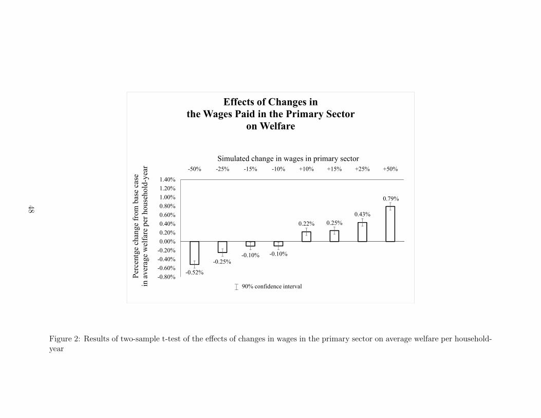
-0.52%

-0.25%-0.10% -0.10%

0.22% 0.25%

0.43%

0.79%

-0.80%

-0.60%

-0.40%

-0.20%

0.00%

0.20%

0.40%

0.60%

0.80%

1.00%

1.20%

1.40%

-50% -25% -15% -10% +10% +15% +25% +50%

Effects of Changes inthe Wages Paid in the Primary Sector

on WelfareP

erce

ntge

chan

ge f

rom

bas

e ca

se

in a

vera

ge w

elfa

re p

er h

ouse

hold

-yea

r

Simulated change in wages in primary sector

90% confidence interval

Figure 2: Results of two-sample t-test of the effects of changes in wages in the primary sector on average welfare per household-year

48

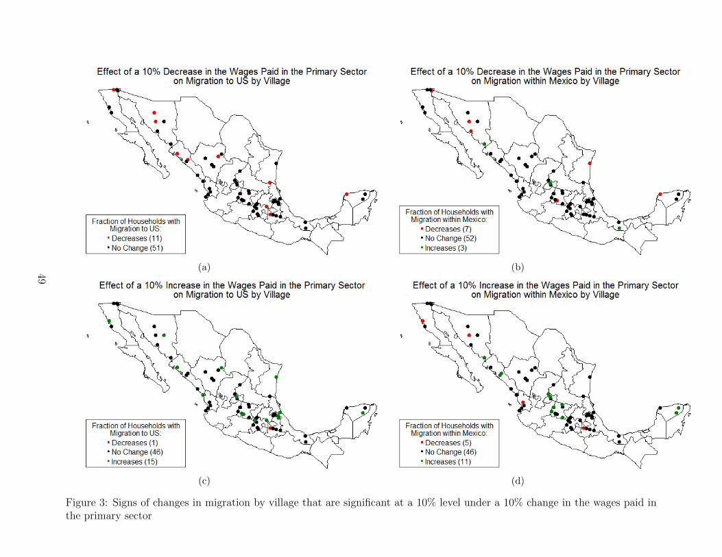
(a) (b)

(c) (d)

Figure 3: Signs of changes in migration by village that are significant at a 10% level under a 10% change in the wages paid inthe primary sector

49

Table 2: Effects of Changes in the Wages Paid in the Primary Sector:Determinants of significant changes at the village level

in the fraction of households with migration

Dependent variable is the value of significant changes in the fraction of households with migration to/within:US Mexico US Mexico

Simulated change in wages in primary sector: 10% Increase 10% Decrease

Characteristics from the initial year of the simulation (1997):Distance to closest border crossing point (1000 km) -0.0012 0.0102*** 0.0020 0.0016

(0.0055) (0.0037) (0.0037) (0.0046)Crime rate at closest border crossing point -0.0002 -0.0002 0.0003 -0.0001

(0.0005) (0.0003) (0.0003) (0.0004)Employment in primary sector 0.0001 0.0000 -0.0000 0.0003

(0.0004) (0.0002) (0.0002) (0.0003)Employment in secondary sector 0.0004 -0.0000 -0.0001 -0.0005

(0.0006) (0.0004) (0.0004) (0.0005)Number of males in household 0.0012 0.0092* -0.0010 0.0091

(0.0080) (0.0053) (0.0053) (0.0066)Household head age 0.0004 0.0007* -0.0004 0.0003

(0.0006) (0.0004) (0.0004) (0.0005)Household head schooling 0.0033 -0.0018 -0.0049** 0.0003

(0.0036) (0.0024) (0.0024) (0.0030)Number of household members -0.0048 -0.0074** -0.0016 -0.0033

(0.0053) (0.0035) (0.0035) (0.0044)Fraction of households with migration to US 0.0180 0.0102 0.0032 -0.0002

(0.0151) (0.0101) (0.0101) (0.0125)Fraction of households with migration within Mexico 0.0448* -0.0031 0.0184 -0.0225

(0.0230) (0.0153) (0.0154) (0.0191)Household average schooling -0.0017 -0.0006 0.0045* -0.0026

(0.0039) (0.0026) (0.0026) (0.0032)Household land quality (1=good, 4=very bad) 0.0005 0.0038 -0.0013 -0.0043

(0.0056) (0.0038) (0.0038) (0.0047)Constant -0.0105 -0.0173 0.0154 0.0218

(0.0470) (0.0313) (0.0314) (0.0390)

p-value (Pr>F) 0.8550 0.1480 0.4930 0.2520# observations 62 62 62 62Notes: Standard errors in parentheses. To analyze the determinants of significant changes at the villagelevel in the fraction of households with migration, we regress the village-level changes in the fraction ofhouseholds with migration over the entire simulation period (1997-2007) that are significant at a 10% levelunder a simulated 10% increase and a simulated 10% decrease in primary sector wages in the initial yearof the simulation (1997), respectively, on the initial village, municipality, state, and national characteristicsfrom the initial year of the simulation (1997). Crime rates are in homicides per 10,000 inhabitants.Significance codes: * p<0.10, ** p<0.05, *** p<0.01.

50

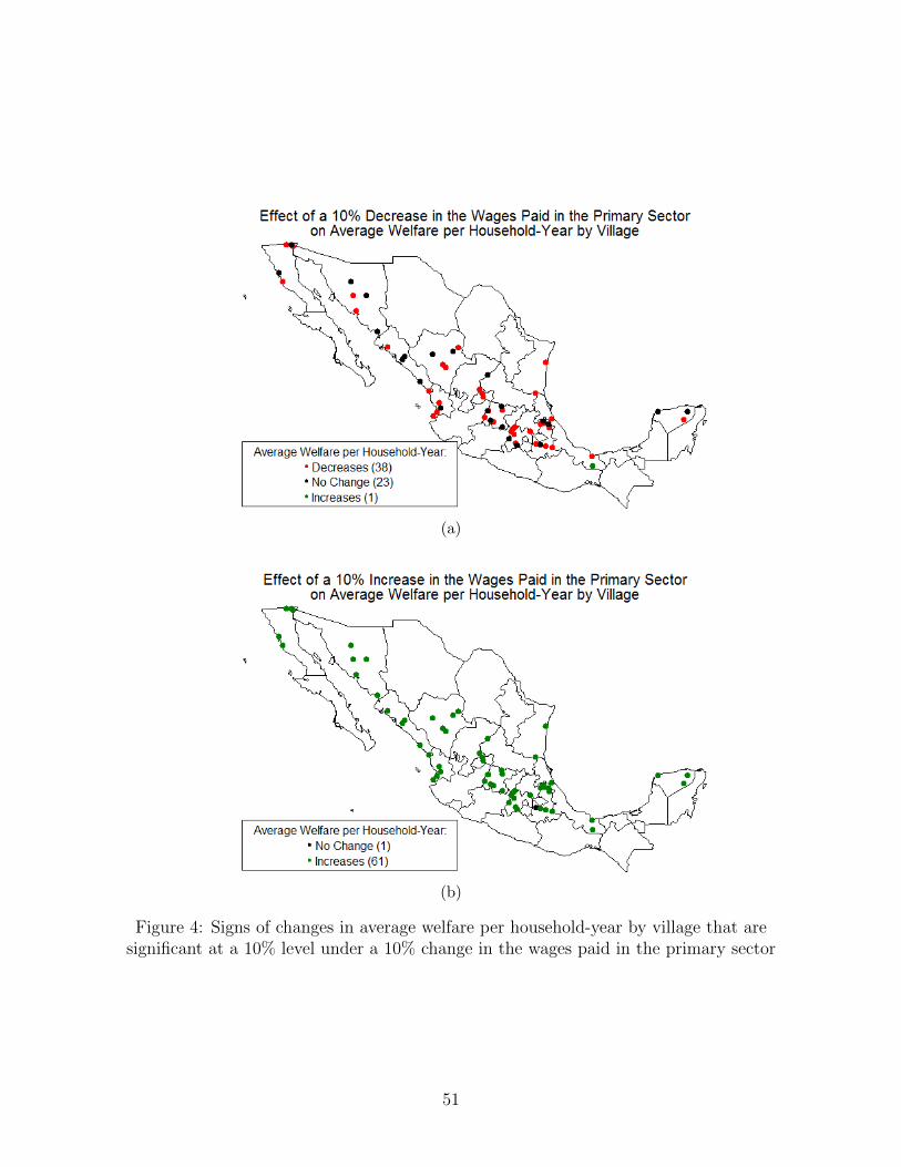
(a)

(b)

Figure 4: Signs of changes in average welfare per household-year by village that aresignificant at a 10% level under a 10% change in the wages paid in the primary sector

51

-10.9%

-28.0%

-39.2%-43.7%

-63.5%-68.5%

-77.0%

-89.5%

-0.5% -1.9% -3.1% -3.5% -4.1% -4.8% -5.8% -7.1%

-100%

-90%

-80%

-70%

-60%

-50%

-40%

-30%

-20%

-10%

0%

10%

50% 75% 85% 90% 110% 115% 125% 150%

Effects of a

Minimum Threshold Household Average Schooling

Needed for Migration to US

on Migration

to US within Mexico

Per

centg

ech

ange

from

bas

e ca

se i

n

frac

tio

n o

f h

ou

seh

old

s w

ith

mig

rati

on

Minimum as % of mean household average schooling

90% confidence interval

Figure 5: Results of two-sample t-test of the effects of a minimum threshold household average schooling needed for migrationto US on the fraction of households with migration

52

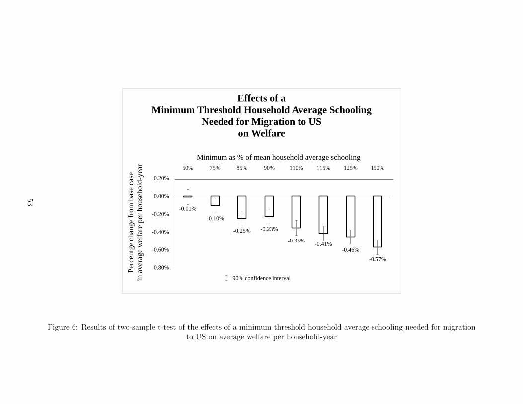
-0.01%

-0.10%

-0.25% -0.23%

-0.35%-0.41%

-0.46%

-0.57%

-0.80%

-0.60%

-0.40%

-0.20%

0.00%

0.20%

50% 75% 85% 90% 110% 115% 125% 150%

Effects of a

Minimum Threshold Household Average Schooling

Needed for Migration to US

on WelfareP

erce

ntg

ech

ange

from

bas

e ca

se

in a

ver

age

wel

fare

per

house

hold

-yea

r

Minimum as % of mean household average schooling

90% confidence interval

Figure 6: Results of two-sample t-test of the effects of a minimum threshold household average schooling needed for migrationto US on average welfare per household-year

53

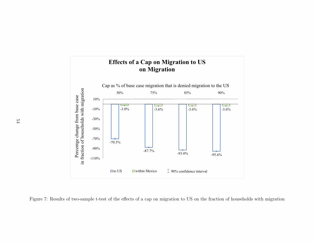
-70.3%

-87.7%-93.0% -95.6%

-3.0% -3.6% -3.6% -3.6%

-110%

-90%

-70%

-50%

-30%

-10%

10%

50% 75% 85% 90%

Effects of a Cap on Migration to USon Migration

to US within Mexico

Perc

entg

ech

ange

fro

m b

ase

case

in

fra

ctio

n of

hou

seho

lds

wit

h m

igra

tion

Cap as % of base case migration that is denied migration to the US

90% confidence interval

Figure 7: Results of two-sample t-test of the effects of a cap on migration to US on the fraction of households with migration

54

-0.39%

-0.51% -0.53%-0.55%

-0.80%

-0.70%

-0.60%

-0.50%

-0.40%

-0.30%

-0.20%

-0.10%

0.00%

0.10%

50% 75% 85% 90%

Effects of a Cap on Migration to the USon Welfare

Per

cent

gech

ange

fro

m b

ase

case

in

ave

rage

wel

fare

per

hou

seho

ld-y

ear

Cap as % of base case migration that is denied migration to the US

90% confidence interval

Figure 8: Results of two-sample t-test of the effects of a cap on migration to US on average welfare per household-year

55

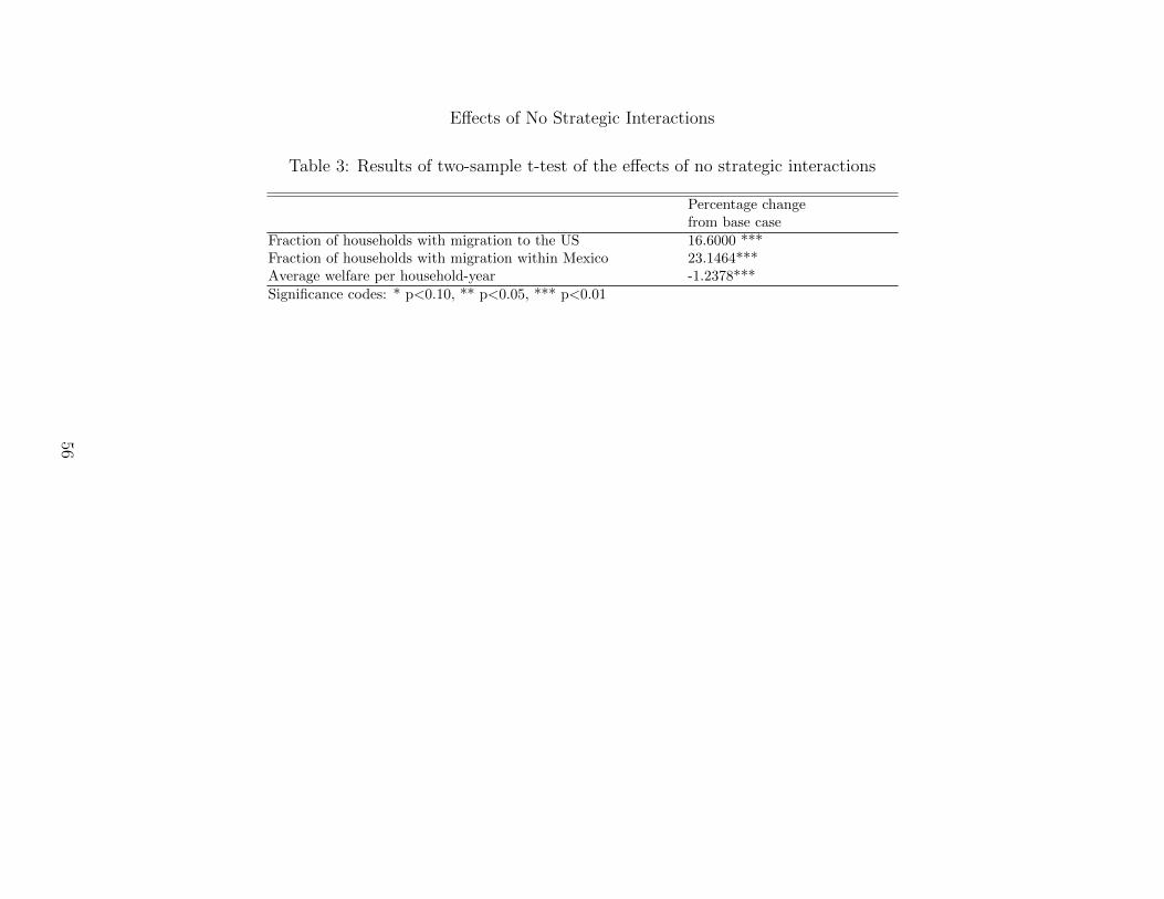
Effects of No Strategic Interactions

Table 3: Results of two-sample t-test of the effects of no strategic interactions

Percentage changefrom base case

Fraction of households with migration to the US 16.6000 ***Fraction of households with migration within Mexico 23.1464***Average welfare per household-year -1.2378***

Significance codes: * p<0.10, ** p<0.05, *** p<0.01

56

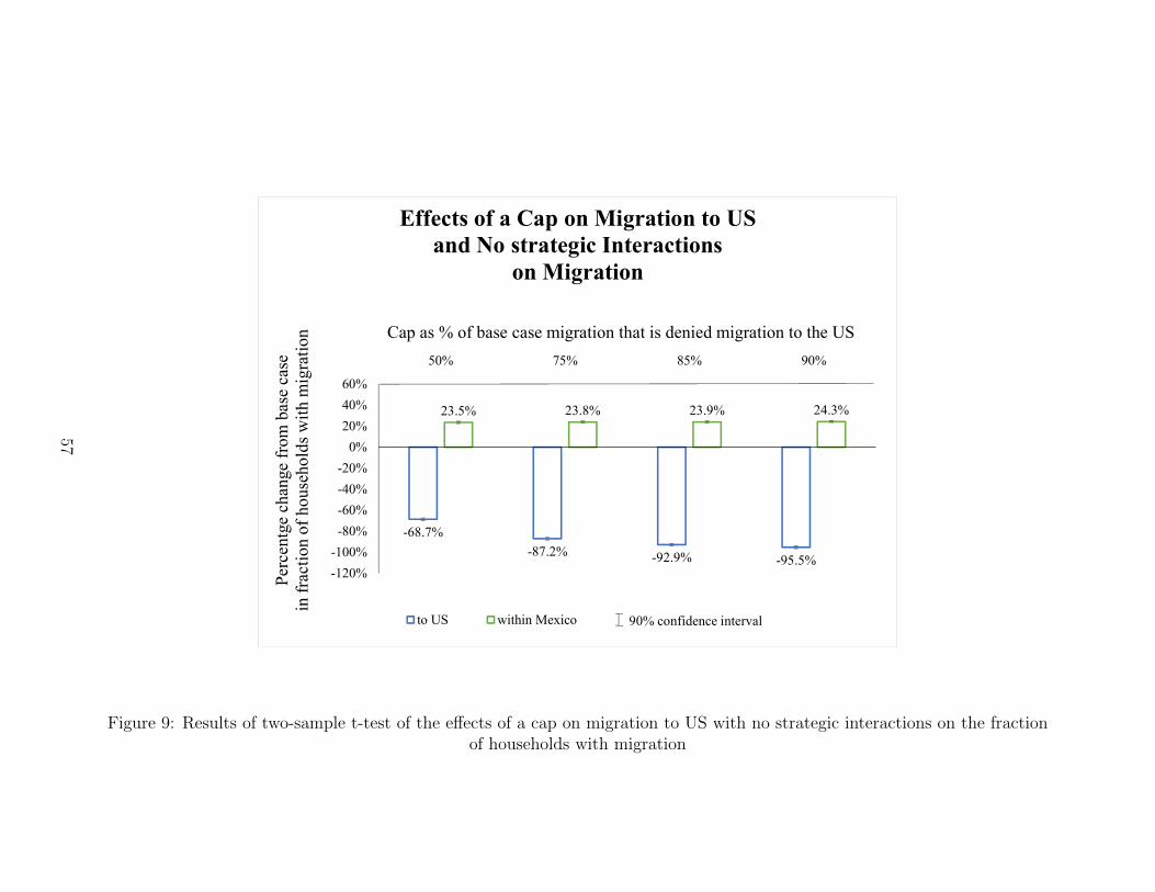
-68.7%

-87.2% -92.9% -95.5%

23.5% 23.8% 23.9% 24.3%

-120%

-100%

-80%

-60%

-40%

-20%

0%

20%

40%

60%

50% 75% 85% 90%

Effects of a Cap on Migration to USand No strategic Interactions

on Migration

to US within Mexico

Perc

entg

ech

ange

fro

m b

ase

case

in

fra

ctio

n of

hou

seho

lds

wit

h m

igra

tion Cap as % of base case migration that is denied migration to the US

90% confidence interval

Figure 9: Results of two-sample t-test of the effects of a cap on migration to US with no strategic interactions on the fractionof households with migration

57

Effects of No Dynamic Behavior

Table 4: Results of two-sample t-test of the effects of no dynamic behavior

Percentage changefrom base case

Fraction of households with migration to the US -63.3507***Fraction of households with migration within Mexico -63.1481***Average welfare per household-year -65.3700***

Significance codes: * p<0.10, ** p<0.05, *** p<0.01

58

-81.7%-90.8% -94.4% -96.3%

-63.3% -63.3% -63.3% -62.9%

-120%

-100%

-80%

-60%

-40%

-20%

0%

20%

50% 75% 85% 90%

Effects of a Cap on Migration to USand No Dynamic Behavior

on Migration

to US within Mexico

Perc

entg

ech

ange

fro

m b

ase

case

in

fra

ctio

n of

hou

seho

lds

wit

h m

igra

tion Cap as % of base case migration that is denied migration to the US

90% confidence interval

Figure 10: Results of two-sample t-test of the effects of a cap on migration to US with no dynamic behavior on the fraction ofhouseholds with migration

59

Appendix A. Supplementary Tables and Figures

!

!!

!

!!

!

!

!

!

!

!

!

!

!

!

!!

!!!!!! !

!!

! !

!

!

!!

!!

!!!!

!

!!!

!

!!

!

!

!

!

!!!

!

!

!

!

!!

!

!

!

!

! !!

!

!!

!

!!

!!

!

!

!

!!

!

DD DDD DD DD D

D DDD

D DD

DDDDDDDDD

¯

Legend:

D US - Mexico border crossing points! ENHRUM sampled localites

Figure A.1: Location of sampled villages in the ENHRUM survey and the border crossingmunicipalities

60

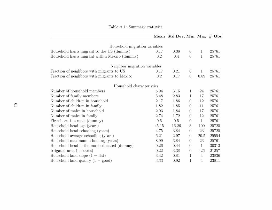
Table A.1: Summary statistics

Mean Std.Dev. Min Max # Obs

Household migration variablesHousehold has a migrant to the US (dummy) 0.17 0.38 0 1 25761Household has a migrant within Mexico (dummy) 0.2 0.4 0 1 25761

Neighbor migration variablesFraction of neighbors with migrants to US 0.17 0.21 0 1 25761Fraction of neighbors with migrants to Mexico 0.2 0.17 0 0.89 25761

Household characteristicsNumber of household members 5.94 3.15 1 24 25761Number of family members 5.48 2.83 1 17 25761Number of children in household 2.17 1.86 0 12 25761Number of children in family 1.82 1.85 0 11 25761Number of males in household 2.93 1.84 0 17 25761Number of males in family 2.74 1.72 0 12 25761First born is a male (dummy) 0.5 0.5 0 1 25761Household head age (years) 45.15 16.26 3 100 25725Household head schooling (years) 4.75 3.84 0 23 25725Household average schooling (years) 6.21 2.97 0 20.5 25554Household maximum schooling (years) 8.99 3.84 0 23 25761Household head is the most educated (dummy) 0.26 0.44 0 1 30313Irrigated area (hectares) 0.22 3.38 0 426 21257Household land slope (1 = flat) 3.42 0.81 1 4 23836Household land quality (1 = good) 3.33 0.92 1 4 23811

61

Table A.1: (continued)

Mean Std.Dev. Min Max # ObsMunicipality characteristics

Number of basic schools 284.97 332.44 0 1762 22763Number of indigenous schools 6.08 12.78 0 72 23313Number of schools 238.87 301.17 0 1603 13107Number of classrooms 1399.33 2236.64 0 12707 13322Number of public libraries 20.09 34.74 0 327 11523Number of labs 47.84 82.72 0 482 12987Number of workshops 42.78 69.6 0 424 12987Number of public libraries 4.92 5.69 0 28 19165Number of students 42284.31 70057.57 0 372625 22763Number of vehicles 44556.99 88624.85 0 502836 24220Number of cars 29396.74 64269.9 0 383512 24220Number of buses 371.1 841.11 0 5355 24220Number of trucks 14203.43 23759.15 0 113819 24220Number of motos 585.72 1685.87 0 18650 24220

State-level variablesEmployment in primary sector (% working population) 20.3 10.37 4.3 52 20635Employment in secondary sector (% working population) 26.58 6.03 15.1 40.7 20635Employment in tertiaty sector (% working population) 52.78 7.14 31.6 68.1 20635

National variablesHourly wage in primary sector (2010 Mexican pesos) 29.48 5.3 21.91 39.45 30313Hourly wage in secondary sector (2010 Mexican pesos) 31.77 3.4 24.9 35.98 30313Hourly wage in tertiary sector (2010 Mexican pesos) 37.81 4.21 30.27 43.54 30313Average hourly wage (2010 Mexican pesos) 35.97 3.34 29.61 41.44 33873

Border crossing variablesDistance to the closest border crossing point (km) 847.4 474.1 7.0 2178.3 30352

62

Table A.1: (continued)

Mean Std.Dev. Min Max # Obs

Number of border crossing points... < 1000 km 6.3 5.4 0.0 17.0 30352... 1000-2000 km 12.4 6.0 0.0 26.0 30352

Average crime rate (murders per 10,000 inhabitants)... in crossing municipalities < 1000 km 11.5 8.8 1.9 83.7 12166... in crossing municipalities 1000-2000 km 12.2 7.4 2.9 52.3 16612... along border municipalities 14.3 2.5 9.9 18.4 17554... at the closest crossing point 8.7 6.6 0.0 38.2 17554... at the second closest crossing point 13.8 26.3 0.0 217.4 17554... at the third closest crossing point 9.6 19.2 0.0 144.2 17554

63

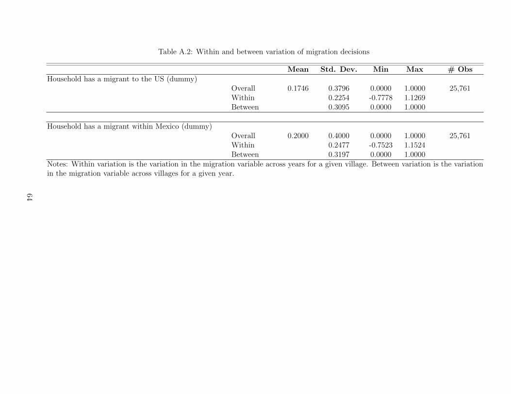
Table A.2: Within and between variation of migration decisions

Mean Std. Dev. Min Max # ObsHousehold has a migrant to the US (dummy)

Overall 0.1746 0.3796 0.0000 1.0000 25,761Within 0.2254 -0.7778 1.1269Between 0.3095 0.0000 1.0000

Household has a migrant within Mexico (dummy)Overall 0.2000 0.4000 0.0000 1.0000 25,761Within 0.2477 -0.7523 1.1524Between 0.3197 0.0000 1.0000

Notes: Within variation is the variation in the migration variable across years for a given village. Between variation is the variationin the migration variable across villages for a given year.

64

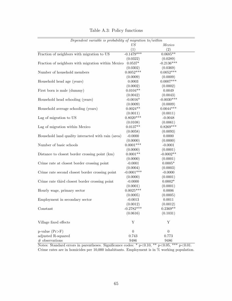
Table A.3: Policy functions

Dependent variable is probability of migration to/withinUS Mexico(1) (2)

Fraction of neighbors with migration to US -0.1479*** 0.0685**(0.0322) (0.0289)

Fraction of neighbors with migration within Mexico 0.0537* -0.2136***(0.0302) (0.0369)

Number of household members 0.0052*** 0.0052***(0.0009) (0.0009)

Household head age (years) 0.0003 0.0007***(0.0002) (0.0002)

First born is male (dummy) 0.0104** 0.0049(0.0042) (0.0043)

Household head schooling (years) -0.0016* -0.0030***(0.0009) (0.0009)

Household average schooling (years) 0.0024** 0.0044***(0.0011) (0.0011)

Lag of migration to US 0.8020*** -0.0048(0.0108) (0.0061)

Lag of migration within Mexico 0.0137** 0.8269***(0.0058) (0.0093)

Household land quality interacted with rain (area) -0.0000 0.0000(0.0000) (0.0000)

Number of basic schools 0.0001*** -0.0001(0.0000) (0.0001)

Distance to closest border crossing point (km) 0.0001** -0.0002**(0.0000) (0.0001)

Crime rate at closest border crossing point -0.0001 0.0005*(0.0004) (0.0003)

Crime rate second closest border crossing point -0.0001*** -0.0000(0.0000) (0.0001)

Crime rate third closest border crossing point -0.0000 0.0002*(0.0001) (0.0001)

Hourly wage, primary sector 0.0025*** 0.0006(0.0005) (0.0005)

Employment in secondary sector -0.0013 0.0011(0.0012) (0.0012)

Constant -0.2782*** 0.2369**(0.0616) (0.1031)

Village fixed effects Y Y

p-value (Pr>F) 0 0adjusted R-squared 0.743 0.773# observations 9486 9486Notes: Standard errors in parentheses. Significance codes: * p<0.10, ** p<0.05, *** p<0.01.Crime rates are in homicides per 10,000 inhabitants. Employment is in % working population.

65

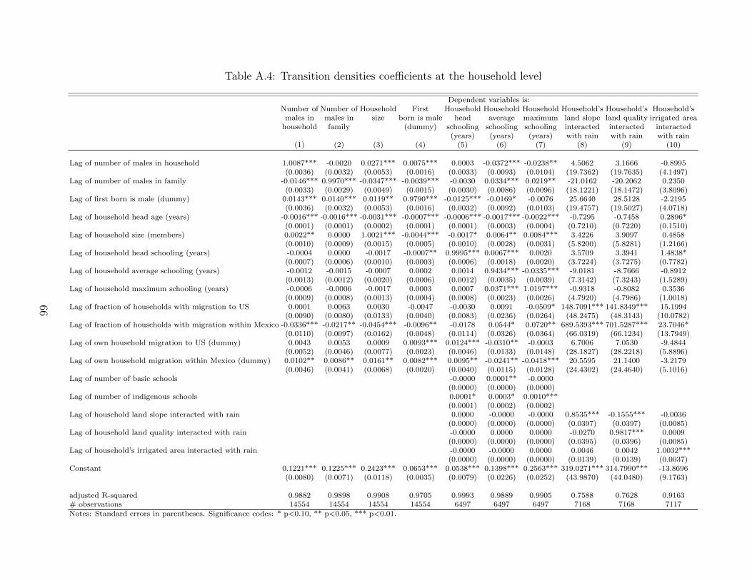
Table A.4: Transition densities coefficients at the household level

Dependent variables is:Number of Number of Household First Household Household Household Household’s Household’s Household’smales in males in size born is male head average maximum land slope land quality irrigated area

household family (dummy) schooling schooling schooling interacted interacted interacted(years) (years) (years) with rain with rain with rain

(1) (2) (3) (4) (5) (6) (7) (8) (9) (10)

Lag of number of males in household 1.0087*** -0.0020 0.0271*** 0.0075*** 0.0003 -0.0372*** -0.0238** 4.5062 3.1666 -0.8995(0.0036) (0.0032) (0.0053) (0.0016) (0.0033) (0.0093) (0.0104) (19.7362) (19.7635) (4.1497)

Lag of number of males in family -0.0146*** 0.9970*** -0.0347*** -0.0039*** -0.0030 0.0334*** 0.0219** -21.0162 -20.2062 0.2350(0.0033) (0.0029) (0.0049) (0.0015) (0.0030) (0.0086) (0.0096) (18.1221) (18.1472) (3.8096)

Lag of first born is male (dummy) 0.0143*** 0.0140*** 0.0119** 0.9790*** -0.0125*** -0.0169* -0.0076 25.6640 28.5128 -2.2195(0.0036) (0.0032) (0.0053) (0.0016) (0.0032) (0.0092) (0.0103) (19.4757) (19.5027) (4.0718)

Lag of household head age (years) -0.0016*** -0.0016*** -0.0031*** -0.0007*** -0.0006*** -0.0017*** -0.0022*** -0.7295 -0.7458 0.2896*(0.0001) (0.0001) (0.0002) (0.0001) (0.0001) (0.0003) (0.0004) (0.7210) (0.7220) (0.1510)

Lag of household size (members) 0.0022** 0.0000 1.0021*** -0.0044*** -0.0017* 0.0064** 0.0084*** 3.4226 3.9097 0.4858(0.0010) (0.0009) (0.0015) (0.0005) (0.0010) (0.0028) (0.0031) (5.8200) (5.8281) (1.2166)

Lag of household head schooling (years) -0.0004 0.0000 -0.0017 -0.0007** 0.9995*** 0.0067*** 0.0020 3.5709 3.3941 1.4838*(0.0007) (0.0006) (0.0010) (0.0003) (0.0006) (0.0018) (0.0020) (3.7224) (3.7275) (0.7782)

Lag of household average schooling (years) -0.0012 -0.0015 -0.0007 0.0002 0.0014 0.9434*** -0.0335*** -9.0181 -8.7666 -0.8912(0.0013) (0.0012) (0.0020) (0.0006) (0.0012) (0.0035) (0.0039) (7.3142) (7.3243) (1.5289)

Lag of household maximum schooling (years) -0.0006 -0.0006 -0.0017 0.0003 0.0007 0.0371*** 1.0197*** -0.9318 -0.8082 0.3536(0.0009) (0.0008) (0.0013) (0.0004) (0.0008) (0.0023) (0.0026) (4.7920) (4.7986) (1.0018)

Lag of fraction of households with migration to US 0.0001 0.0063 0.0030 -0.0047 -0.0030 0.0091 -0.0509* 148.7091*** 141.8349*** 15.1994(0.0090) (0.0080) (0.0133) (0.0040) (0.0083) (0.0236) (0.0264) (48.2475) (48.3143) (10.0782)

Lag of fraction of households with migration within Mexico -0.0336*** -0.0217** -0.0454*** -0.0096** -0.0178 0.0544* 0.0720** 689.5393*** 701.5287*** 23.7046*(0.0110) (0.0097) (0.0162) (0.0048) (0.0114) (0.0326) (0.0364) (66.0319) (66.1234) (13.7949)

Lag of own household migration to US (dummy) 0.0043 0.0053 0.0009 0.0093*** 0.0124*** -0.0310** -0.0003 6.7006 7.0530 -9.4844(0.0052) (0.0046) (0.0077) (0.0023) (0.0046) (0.0133) (0.0148) (28.1827) (28.2218) (5.8896)

Lag of own household migration within Mexico (dummy) 0.0102** 0.0086** 0.0161** 0.0082*** 0.0095** -0.0241** -0.0418*** 20.5595 21.1400 -3.2179(0.0046) (0.0041) (0.0068) (0.0020) (0.0040) (0.0115) (0.0128) (24.4302) (24.4640) (5.1016)

Lag of number of basic schools -0.0000 0.0001** -0.0000(0.0000) (0.0000) (0.0000)

Lag of number of indigenous schools 0.0001* 0.0003* 0.0010***(0.0001) (0.0002) (0.0002)

Lag of household land slope interacted with rain 0.0000 -0.0000 -0.0000 0.8535*** -0.1555*** -0.0036(0.0000) (0.0000) (0.0000) (0.0397) (0.0397) (0.0085)

Lag of household land quality interacted with rain -0.0000 0.0000 0.0000 -0.0270 0.9817*** 0.0009(0.0000) (0.0000) (0.0000) (0.0395) (0.0396) (0.0085)

Lag of household’s irrigated area interacted with rain -0.0000 -0.0000 0.0000 0.0046 0.0042 1.0032***(0.0000) (0.0000) (0.0000) (0.0139) (0.0139) (0.0037)

Constant 0.1221*** 0.1225*** 0.2423*** 0.0653*** 0.0538*** 0.1398*** 0.2563*** 319.0271*** 314.7990*** -13.8696(0.0080) (0.0071) (0.0118) (0.0035) (0.0079) (0.0226) (0.0252) (43.9870) (44.0480) (9.1763)

adjusted R-squared 0.9882 0.9898 0.9908 0.9705 0.9993 0.9889 0.9905 0.7588 0.7628 0.9163# observations 14554 14554 14554 14554 6497 6497 6497 7168 7168 7117Notes: Standard errors in parentheses. Significance codes: * p<0.10, ** p<0.05, *** p<0.01.

66

Table A.5: Transition densities coefficients at the village and municipality level

Dependent variable is:Crime at closest Crime at second Crime at third Number of Number of Number of

crossing border point crossing border point crossing border point basic schools indigenous schools students inbasic system

(11) (12) (13) (14) (15) (16)

Lag of number of basic schools 0.5484*** 0.0003 27.0023***(0.0431) (0.0073) (3.9734)

Lag of number of indigenous schools -0.2278 0.4956*** -14.9978(0.2207) (0.0372) (20.3280)

Lag of number of students in basic system 0.0009* -0.0001 0.0941**(0.0004) (0.0001) (0.0413)

Lag of employment in primary sector 1.0530 0.0180 -18.8602(1.2750) (0.2160) (117.4470)

Lag of employment in secondary sector 1.3148 -0.0555 -51.5847(1.2895) (0.2188) (118.7885)

Lag of employment in tertiary sector 0.7357 -0.0007 10.5247(1.3240) (0.2243) (121.9671)

Lag of avg. hourly wage in primary sector (pesos) -0.5765*** 4.2476*** 0.4092(0.1314) (0.8395) (0.3101)

Lag of avg. hourly wage in secondary sector (pesos) -2.0471*** 0.3548 0.3891(0.2333) (1.4910) (0.5507)

Lag of avg. hourly wage in tertiary sector (pesos) 1.9010*** -2.6400 -0.9146(0.2633) (1.6822) (0.6213)

Lag of crime at closest border crossing point 0.3543*** 0.9985*** 0.3662***(0.0285) (0.1822) (0.0673)

Lag of crime at second closest border crossing point 0.0347*** 0.2047*** 0.0389***(0.0050) (0.0321) (0.0118)

Lag of crime at third closest border crossing point 0.0850*** 0.4031*** 0.1935***(0.0142) (0.0909) (0.0336)

Constant 17.2215*** -33.4177* 15.3372** -35.3086 8.6043 19691.8306*(3.1505) (20.1307) (7.4350) (126.5089) (21.4457) (11653.7577)

adjusted R-squared 0.3736 0.1547 0.1001 0.9814 0.9907 0.7589# observations 960 960 960 743 735 743

Notes: Standard errors in parentheses. Employment is in % working population. Crime is in homicides per 10,000 inhabitants.Significance codes: * p<0.10, ** p<0.05, *** p<0.01.

67

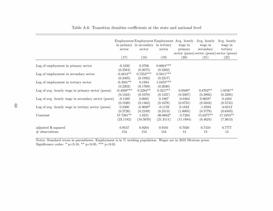
Table A.6: Transition densities coefficients at the state and national level

Employment Employment Employment Avg. hourly Avg. hourly Avg. hourlyin primary in secondary in tertiary wage in wage in wage in

sector sector sector primary secondary tertiarysector (pesos) sector (pesos) sector (pesos)

(17) (18) (19) (20) (21) (22)

Lag of employment in primary sector -0.1632 0.2706 0.6664***(0.2584) (0.2075) (0.2382)

Lag of employment in secondary sector -0.4812** 0.7253*** 0.5811***(0.2405) (0.1932) (0.2217)

Lag of employment in tertiary sector -0.4501** 0.1884 1.0455***(0.2202) (0.1769) (0.2030)

Lag of avg. hourly wage in primary sector (pesos) -0.4508*** 0.2284** 0.3217** 0.9509* 0.8702** 1.0556**(0.1342) (0.1078) (0.1237) (0.5007) (0.2892) (0.3295)

Lag of avg. hourly wage in secondary sector (pesos) -0.1500 0.0685 0.1867 -0.0404 0.9658* 0.4484(0.1820) (0.1462) (0.1678) (0.8731) (0.5043) (0.5745)

Lag of avg. hourly wage in tertiary sector (pesos) 0.2400 -0.3680* -0.1159 0.1823 -1.0594 -0.6512(0.2726) (0.2189) (0.2513) (1.0005) (0.5779) (0.6583)

Constant 57.7381** 1.0251 -36.6682* -2.7204 15.6277** 17.2455**(23.1182) (18.5670) (21.3111) (11.1884) (6.4624) (7.3613)

adjusted R-squared 0.9547 0.9204 0.9101 0.7020 0.7410 0.7777# observations 154 154 154 12 12 12

Notes: Standard errors in parentheses. Employment is in % working population. Wages are in 2010 Mexican pesos.Significance codes: * p<0.10, ** p<0.05, *** p<0.01.

68

Table A.7: Summary of welfare based on actual and simulated data

Estimate Standard error

Actual average welfare per household year based on:Actual data -0.017739 0.14013Simulated data -0.012241 0.00004***

Notes: Standard errors in parentheses. Significance codes: * p<0.10,** p<0.05, *** p<0.01

69

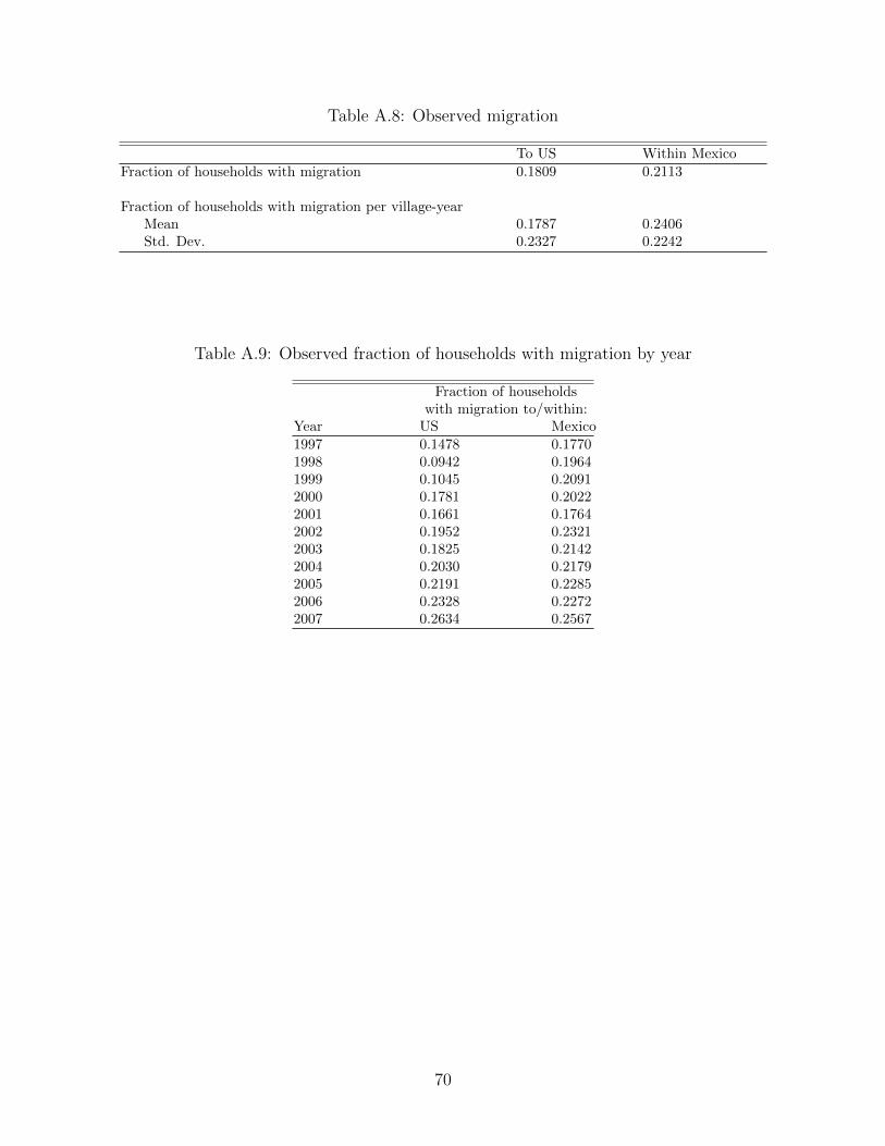
Table A.8: Observed migration

To US Within Mexico

Fraction of households with migration 0.1809 0.2113

Fraction of households with migration per village-yearMean 0.1787 0.2406Std. Dev. 0.2327 0.2242

Table A.9: Observed fraction of households with migration by year

Fraction of householdswith migration to/within:

Year US Mexico

1997 0.1478 0.17701998 0.0942 0.19641999 0.1045 0.20912000 0.1781 0.20222001 0.1661 0.17642002 0.1952 0.23212003 0.1825 0.21422004 0.2030 0.21792005 0.2191 0.22852006 0.2328 0.22722007 0.2634 0.2567

70

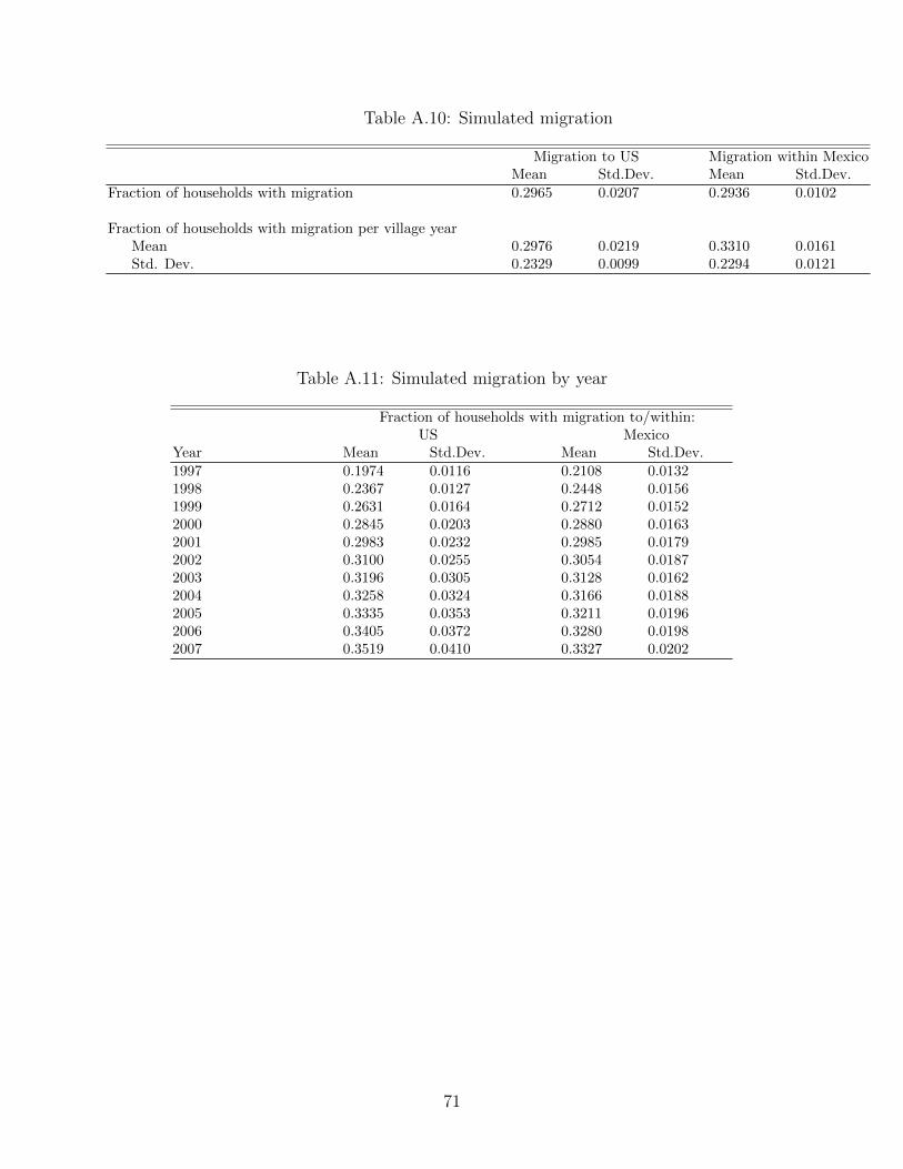
Table A.10: Simulated migration

Migration to US Migration within MexicoMean Std.Dev. Mean Std.Dev.

Fraction of households with migration 0.2965 0.0207 0.2936 0.0102

Fraction of households with migration per village yearMean 0.2976 0.0219 0.3310 0.0161Std. Dev. 0.2329 0.0099 0.2294 0.0121

Table A.11: Simulated migration by year

Fraction of households with migration to/within:US Mexico

Year Mean Std.Dev. Mean Std.Dev.

1997 0.1974 0.0116 0.2108 0.01321998 0.2367 0.0127 0.2448 0.01561999 0.2631 0.0164 0.2712 0.01522000 0.2845 0.0203 0.2880 0.01632001 0.2983 0.0232 0.2985 0.01792002 0.3100 0.0255 0.3054 0.01872003 0.3196 0.0305 0.3128 0.01622004 0.3258 0.0324 0.3166 0.01882005 0.3335 0.0353 0.3211 0.01962006 0.3405 0.0372 0.3280 0.01982007 0.3519 0.0410 0.3327 0.0202

71

Appendix B. Supplementary Counterfactual Simulations

Table B.1: Effects of Changes in the Wages Paid in the Primary Sector:Determinants of significant changes at the village level

in the average welfare per household-year

Dependent variable is the value of significant changes in the average welfare per household-year:

Simulated change in wages in primary sector: 10% Increase 10% Decrease

Characteristics from the initial year of the simulation (1997):Distance to closest border crossing point (1000 km) 0.0003 0.0004

(0.0003) (0.0003)Crime rate at closest border crossing point -0.0184 0.0059

(0.0250) (0.0276)Employment in primary sector 0.0048 0.0282

(0.0176) (0.0194)Employment in secondary sector 0.0084 0.0191

(0.0291) (0.0321)Number of males in household 0.3362 0.7454*

(0.3906) (0.4310)Household head age 0.0472* 0.0892***

(0.0278) (0.0307)Household head schooling -0.1787 -0.2499

(0.1760) (0.1942)Number of household members -0.3348 -0.3094

(0.2575) (0.2841)Fraction of households with migration to US 0.4864 -1.5430*

(0.7390) (0.8154)Fraction of households with migration within Mexico 2.1125* -2.1275*

(1.1273) (1.2439)Household average schooling 0.0739 0.1690

(0.1885) (0.2080)Household land quality (1=good, 4=very bad) -0.1487 0.4680

(0.2758) (0.3044)Constant 1.9611 -7.5317***

(2.2989) (2.5366)

p-value (Pr>F) 0.0350 0.0126# observations 62 62Notes: Standard errors in parentheses. To analyze the determinants of significant changes at the villagelevel in the average welfare per household-year, we regress the village-level changes in the average welfareper household-year over the entire simulation period (1997-2007) that are significant at a 10% level undera simulated 10% increase and a simulated 10% decrease in primary sector wages in the initial year of thesimulation (1997), respectively, on the initial village, municipality, state, and national characteristics fromthe initial year of the simulation (1997). Crime rates are in homicides per 10,000 inhabitants.Significance codes: * p<0.10, ** p<0.05, *** p<0.01.

72

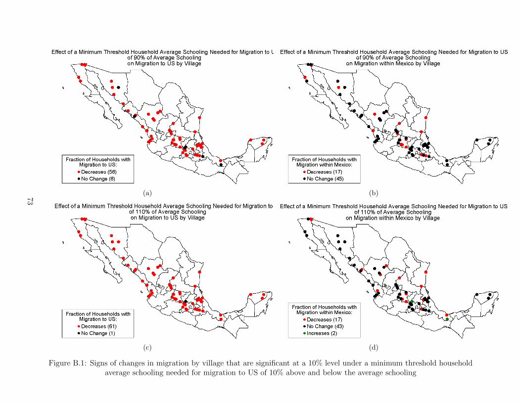
(a) (b)

(c) (d)

Figure B.1: Signs of changes in migration by village that are significant at a 10% level under a minimum threshold householdaverage schooling needed for migration to US of 10% above and below the average schooling

73

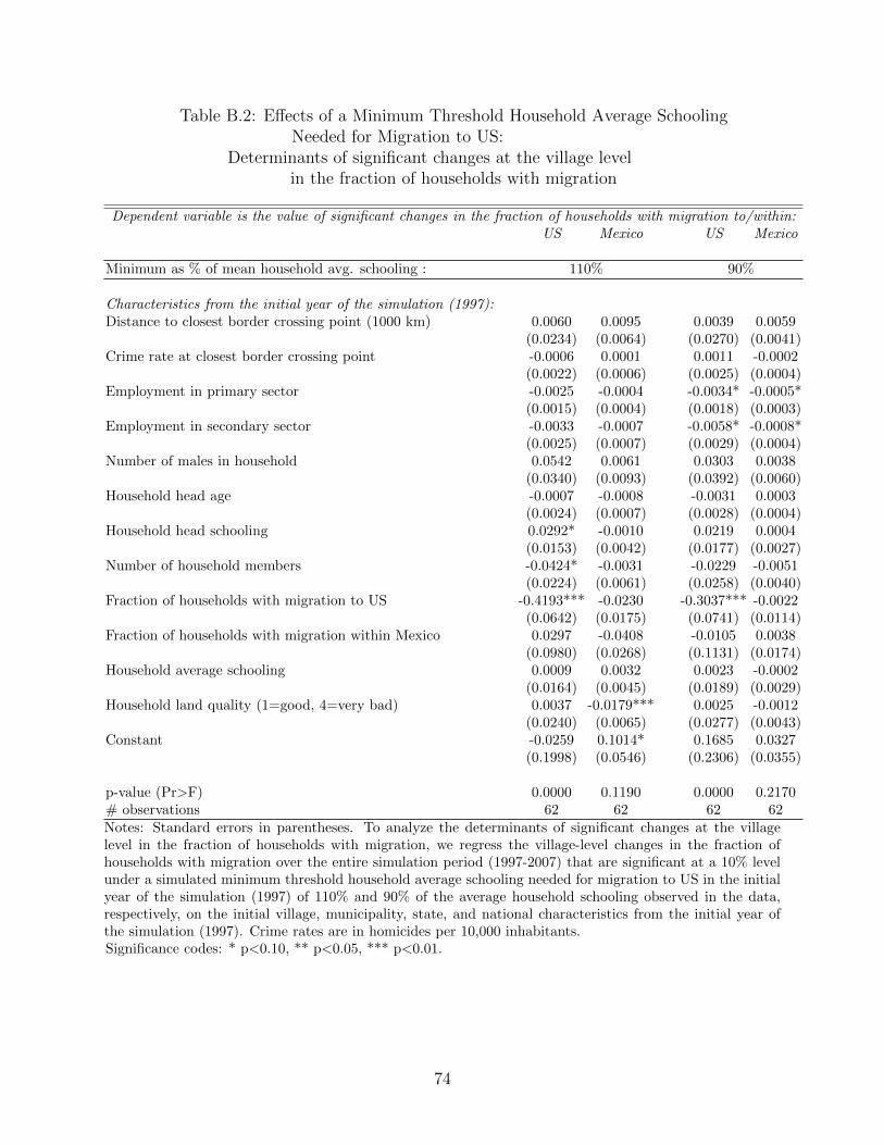
Table B.2: Effects of a Minimum Threshold Household Average SchoolingNeeded for Migration to US:

Determinants of significant changes at the village levelin the fraction of households with migration

Dependent variable is the value of significant changes in the fraction of households with migration to/within:US Mexico US Mexico

Minimum as % of mean household avg. schooling : 110% 90%

Characteristics from the initial year of the simulation (1997):Distance to closest border crossing point (1000 km) 0.0060 0.0095 0.0039 0.0059

(0.0234) (0.0064) (0.0270) (0.0041)Crime rate at closest border crossing point -0.0006 0.0001 0.0011 -0.0002

(0.0022) (0.0006) (0.0025) (0.0004)Employment in primary sector -0.0025 -0.0004 -0.0034* -0.0005*

(0.0015) (0.0004) (0.0018) (0.0003)Employment in secondary sector -0.0033 -0.0007 -0.0058* -0.0008*

(0.0025) (0.0007) (0.0029) (0.0004)Number of males in household 0.0542 0.0061 0.0303 0.0038

(0.0340) (0.0093) (0.0392) (0.0060)Household head age -0.0007 -0.0008 -0.0031 0.0003

(0.0024) (0.0007) (0.0028) (0.0004)Household head schooling 0.0292* -0.0010 0.0219 0.0004

(0.0153) (0.0042) (0.0177) (0.0027)Number of household members -0.0424* -0.0031 -0.0229 -0.0051

(0.0224) (0.0061) (0.0258) (0.0040)Fraction of households with migration to US -0.4193*** -0.0230 -0.3037*** -0.0022

(0.0642) (0.0175) (0.0741) (0.0114)Fraction of households with migration within Mexico 0.0297 -0.0408 -0.0105 0.0038

(0.0980) (0.0268) (0.1131) (0.0174)Household average schooling 0.0009 0.0032 0.0023 -0.0002

(0.0164) (0.0045) (0.0189) (0.0029)Household land quality (1=good, 4=very bad) 0.0037 -0.0179*** 0.0025 -0.0012

(0.0240) (0.0065) (0.0277) (0.0043)Constant -0.0259 0.1014* 0.1685 0.0327

(0.1998) (0.0546) (0.2306) (0.0355)

p-value (Pr>F) 0.0000 0.1190 0.0000 0.2170# observations 62 62 62 62Notes: Standard errors in parentheses. To analyze the determinants of significant changes at the villagelevel in the fraction of households with migration, we regress the village-level changes in the fraction ofhouseholds with migration over the entire simulation period (1997-2007) that are significant at a 10% levelunder a simulated minimum threshold household average schooling needed for migration to US in the initialyear of the simulation (1997) of 110% and 90% of the average household schooling observed in the data,respectively, on the initial village, municipality, state, and national characteristics from the initial year ofthe simulation (1997). Crime rates are in homicides per 10,000 inhabitants.Significance codes: * p<0.10, ** p<0.05, *** p<0.01.

74

(a)

(b)

Figure B.2: Signs of changes in average welfare per household-year by village that aresignificant at a 10% level under a minimum threshold household average schooling needed

for migration to US of 10% above and below the average schooling

75

Table B.3: Effects of a Minimum Threshold Household Average SchoolingNeeded for Migration to US:

Determinants of significant changes at the village levelin the average welfare per household-year

Dependent variable is the value of significant changes in the average welfare per household-year:

Minimum as % of mean household avg. schooling : 110% 90%

Characteristics from the initial year of the simulation (1997):Distance to closest border crossing point (1000 km) 0.0001 -0.0001

(0.0009) (0.0009)Crime rate at closest border crossing point -0.0426 0.0199

(0.0795) (0.0848)Employment in primary sector -0.0733 -0.1102*

(0.0559) (0.0597)Employment in secondary sector -0.1004 -0.1809*

(0.0923) (0.0985)Number of males in household 1.6459 1.0590

(1.2400) (1.3226)Household head age -0.0034 -0.0971

(0.0883) (0.0942)Household head schooling 1.1830** 1.0083*

(0.5588) (0.5960)Number of household members -0.7789 -0.4507

(0.8174) (0.8719)Fraction of households with migration to US -13.3467*** -8.8057***

(2.3461) (2.5024)Fraction of households with migration within Mexico -2.0534 -1.3157

(3.5787) (3.8171)Household average schooling -0.1743 -0.3158

(0.5984) (0.6383)Household land quality (1=good, 4=very bad) 0.1624 0.4884

(0.8757) (0.9340)Constant -2.1404 4.7190

(7.2982) (7.7843)

p-value (Pr>F) 0.0000 0.0000# observations 62 62Notes: Standard errors in parentheses. To analyze the determinants of significant changes at the villagelevel in the average welfare per household-year, we regress the village-level changes in the average welfareper household-year over the entire simulation period (1997-2007) that are significant at a 10% level under asimulated minimum threshold household average schooling needed for migration to US in the initial year ofthe simulation (1997) of 110% and 90% of the average household schooling observed in the data, respectively,on the initial village, municipality, state, and national characteristics from the initial year of the simulation(1997). Crime rates are in homicides per 10,000 inhabitants.Significance codes: * p<0.10, ** p<0.05, *** p<0.01.

76

(a) (b)

Figure B.3: Signs of changes in migration by village that are significant at a 10% level under a cap on migration to US of 90%of base case migration

77

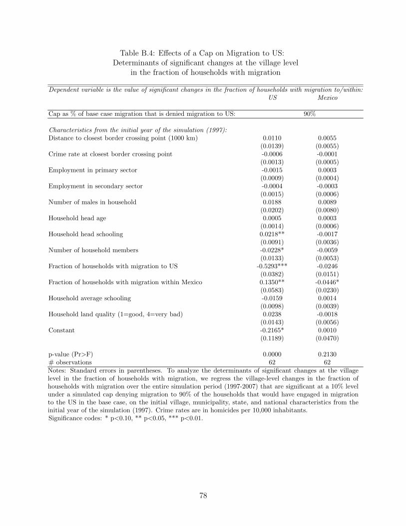
Table B.4: Effects of a Cap on Migration to US:Determinants of significant changes at the village level

in the fraction of households with migration

Dependent variable is the value of significant changes in the fraction of households with migration to/within:US Mexico

Cap as % of base case migration that is denied migration to US: 90%

Characteristics from the initial year of the simulation (1997):Distance to closest border crossing point (1000 km) 0.0110 0.0055

(0.0139) (0.0055)Crime rate at closest border crossing point -0.0006 -0.0001

(0.0013) (0.0005)Employment in primary sector -0.0015 0.0003

(0.0009) (0.0004)Employment in secondary sector -0.0004 -0.0003

(0.0015) (0.0006)Number of males in household 0.0188 0.0089

(0.0202) (0.0080)Household head age 0.0005 0.0003

(0.0014) (0.0006)Household head schooling 0.0218** -0.0017

(0.0091) (0.0036)Number of household members -0.0228* -0.0059

(0.0133) (0.0053)Fraction of households with migration to US -0.5293*** -0.0246

(0.0382) (0.0151)Fraction of households with migration within Mexico 0.1350** -0.0446*

(0.0583) (0.0230)Household average schooling -0.0159 0.0014

(0.0098) (0.0039)Household land quality (1=good, 4=very bad) 0.0238 -0.0018

(0.0143) (0.0056)Constant -0.2165* 0.0010

(0.1189) (0.0470)

p-value (Pr>F) 0.0000 0.2130# observations 62 62Notes: Standard errors in parentheses. To analyze the determinants of significant changes at the villagelevel in the fraction of households with migration, we regress the village-level changes in the fraction ofhouseholds with migration over the entire simulation period (1997-2007) that are significant at a 10% levelunder a simulated cap denying migration to 90% of the households that would have engaged in migrationto the US in the base case, on the initial village, municipality, state, and national characteristics from theinitial year of the simulation (1997). Crime rates are in homicides per 10,000 inhabitants.Significance codes: * p<0.10, ** p<0.05, *** p<0.01.

78

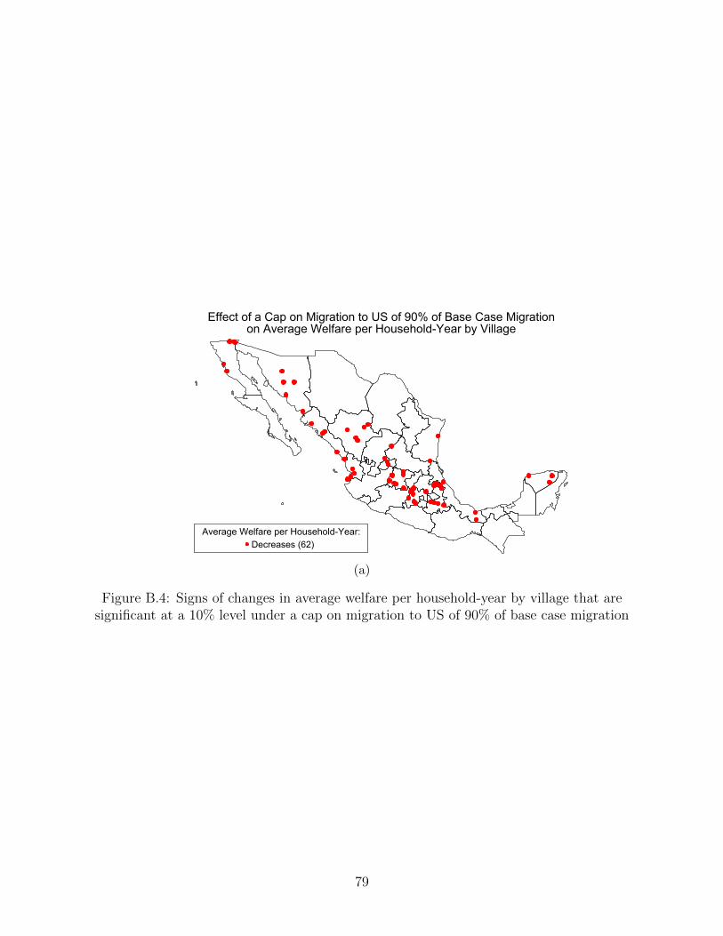
Decreases (62)Average Welfare per Household-Year:

Effect of a Cap on Migration to US of 90% of Base Case Migrationon Average Welfare per Household-Year by Village

(a)

Figure B.4: Signs of changes in average welfare per household-year by village that aresignificant at a 10% level under a cap on migration to US of 90% of base case migration

79

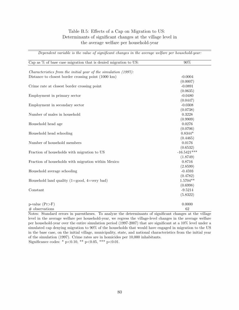
Table B.5: Effects of a Cap on Migration to US:Determinants of significant changes at the village level in

the average welfare per household-year

Dependent variable is the value of significant changes in the average welfare per household-year:

Cap as % of base case migration that is denied migration to US: 90%

Characteristics from the initial year of the simulation (1997):Distance to closest border crossing point (1000 km) -0.0004

(0.0007)Crime rate at closest border crossing point -0.0891

(0.0635)Employment in primary sector -0.0480

(0.0447)Employment in secondary sector -0.0308

(0.0738)Number of males in household 0.3228

(0.9909)Household head age 0.0276

(0.0706)Household head schooling 0.8344*

(0.4465)Number of household members 0.0176

(0.6532)Fraction of households with migration to US -16.5421***

(1.8749)Fraction of households with migration within Mexico 0.8716

(2.8599)Household average schooling -0.4593

(0.4782)Household land quality (1=good, 4=very bad) 1.5704**

(0.6998)Constant -9.5214

(5.8322)

p-value (Pr>F) 0.0000# observations 62Notes: Standard errors in parentheses. To analyze the determinants of significant changes at the villagelevel in the average welfare per household-year, we regress the village-level changes in the average welfareper household-year over the entire simulation period (1997-2007) that are significant at a 10% level under asimulated cap denying migration to 90% of the households that would have engaged in migration to the USin the base case, on the initial village, municipality, state, and national characteristics from the initial yearof the simulation (1997). Crime rates are in homicides per 10,000 inhabitants.Significance codes: * p<0.10, ** p<0.05, *** p<0.01.

80

2.4%1.4% 1.0% 0.9%

0.4%

-0.4%

-1.6% -1.9%

4.1%

1.8% 1.4%0.8%

-0.6%

-0.5%

-1.3%

-2.9%-6%

-4%

-2%

0%

2%

4%

6%

8%

-50% -25% -15% -10% +10% +15% +25% +50%

Effects of Changes inHousehold Head Schooling

on Migration

to US within Mexico

Perc

entg

ech

ange

fro

m b

ase

case

in

frac

tion

of

hous

ehol

ds w

ith

mig

rati

on

Simulated change in household head schooling

90% confidence interval

Figure B.5: Results of two-sample t-test of the effects of changes in household head schooling on the fraction of householdswith migration

81

-0.51%

-0.26%-0.13% -0.07%

0.20%0.26%

0.36%

0.69%

-0.80%

-0.60%

-0.40%

-0.20%

0.00%

0.20%

0.40%

0.60%

0.80%

1.00%

1.20%

-50% -25% -15% -10% +10% +15% +25% +50%

Effects of Changes inHousehold Head Schooling

on WelfareP

erce

ntge

chan

ge f

rom

bas

e ca

se

in a

vera

ge w

elfa

re p

er h

ouse

hold

-yea

r

Simulated change in household head schooling

90% confidence interval

Figure B.6: Results of two-sample t-test of the effects of changes in household head schooling on average welfare perhousehold-year

82

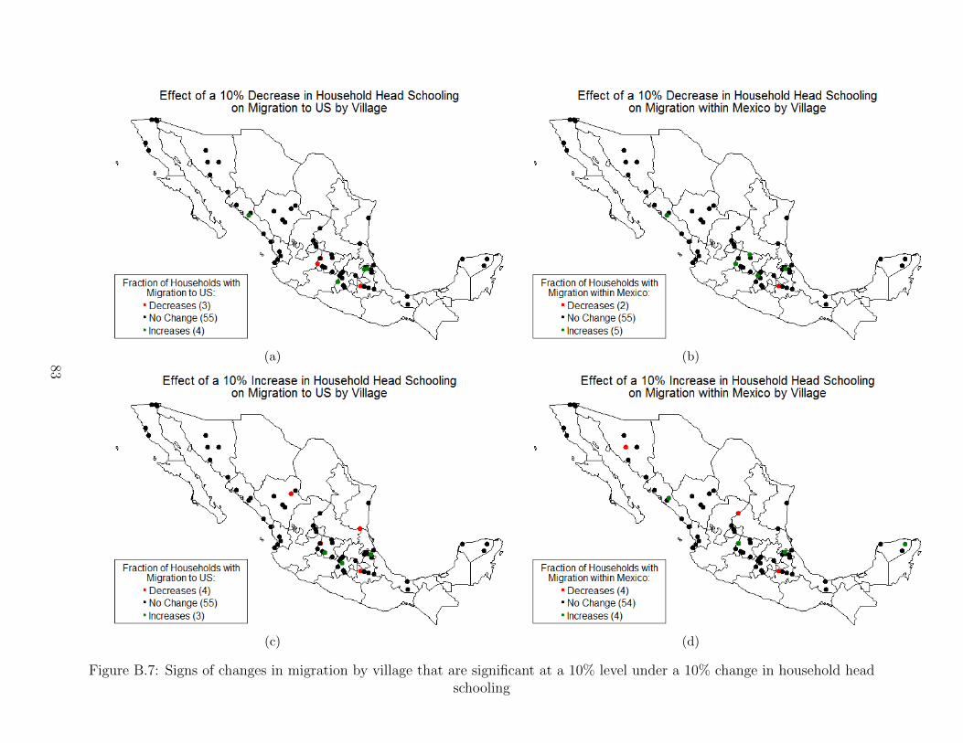
(a) (b)

(c) (d)

Figure B.7: Signs of changes in migration by village that are significant at a 10% level under a 10% change in household headschooling

83

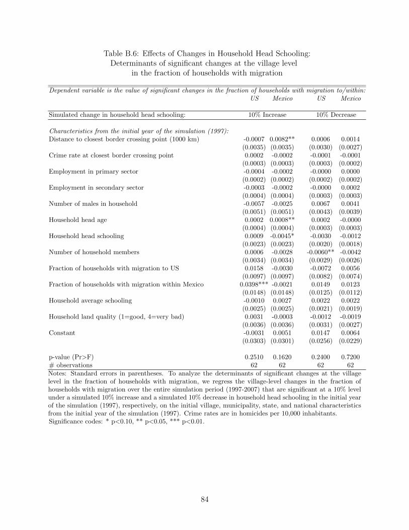
Table B.6: Effects of Changes in Household Head Schooling:Determinants of significant changes at the village level

in the fraction of households with migration

Dependent variable is the value of significant changes in the fraction of households with migration to/within:US Mexico US Mexico

Simulated change in household head schooling: 10% Increase 10% Decrease

Characteristics from the initial year of the simulation (1997):Distance to closest border crossing point (1000 km) -0.0007 0.0082** 0.0006 0.0014

(0.0035) (0.0035) (0.0030) (0.0027)Crime rate at closest border crossing point 0.0002 -0.0002 -0.0001 -0.0001

(0.0003) (0.0003) (0.0003) (0.0002)Employment in primary sector -0.0004 -0.0002 -0.0000 0.0000

(0.0002) (0.0002) (0.0002) (0.0002)Employment in secondary sector -0.0003 -0.0002 -0.0000 0.0002

(0.0004) (0.0004) (0.0003) (0.0003)Number of males in household -0.0057 -0.0025 0.0067 0.0041

(0.0051) (0.0051) (0.0043) (0.0039)Household head age 0.0002 0.0008** 0.0002 -0.0000

(0.0004) (0.0004) (0.0003) (0.0003)Household head schooling 0.0009 -0.0045* -0.0030 -0.0012

(0.0023) (0.0023) (0.0020) (0.0018)Number of household members 0.0006 -0.0028 -0.0060** -0.0042

(0.0034) (0.0034) (0.0029) (0.0026)Fraction of households with migration to US 0.0158 -0.0030 -0.0072 0.0056

(0.0097) (0.0097) (0.0082) (0.0074)Fraction of households with migration within Mexico 0.0398*** -0.0021 0.0149 0.0123

(0.0148) (0.0148) (0.0125) (0.0112)Household average schooling -0.0010 0.0027 0.0022 0.0022

(0.0025) (0.0025) (0.0021) (0.0019)Household land quality (1=good, 4=very bad) 0.0031 -0.0003 -0.0012 -0.0019

(0.0036) (0.0036) (0.0031) (0.0027)Constant -0.0031 0.0051 0.0147 0.0064

(0.0303) (0.0301) (0.0256) (0.0229)

p-value (Pr>F) 0.2510 0.1620 0.2400 0.7200# observations 62 62 62 62Notes: Standard errors in parentheses. To analyze the determinants of significant changes at the villagelevel in the fraction of households with migration, we regress the village-level changes in the fraction ofhouseholds with migration over the entire simulation period (1997-2007) that are significant at a 10% levelunder a simulated 10% increase and a simulated 10% decrease in household head schooling in the initial yearof the simulation (1997), respectively, on the initial village, municipality, state, and national characteristicsfrom the initial year of the simulation (1997). Crime rates are in homicides per 10,000 inhabitants.Significance codes: * p<0.10, ** p<0.05, *** p<0.01.

84

(a)

(b)

Figure B.8: Signs of changes in average welfare per household-year by village that aresignificant at a 10% level under a 10% change in household head schooling

85

Table B.7: Effects of Changes in Household Head Schooling:Determinants of significant changes at the village level

in the average welfare per household-year

Dependent variable is the value of significant changes in the average welfare per household-year:

Simulated change in household head schooling: 10% Increase 10% Decrease

Characteristics from the initial year of the simulation (1997):Distance to closest border crossing point (1000 km) 0.0001 -0.0004

(0.0004) (0.0003)Crime rate at closest border crossing point 0.0140 -0.0196

(0.0353) (0.0286)Employment in primary sector 0.0045 0.0202

(0.0248) (0.0201)Employment in secondary sector -0.0078 0.0288

(0.0410) (0.0332)Number of males in household 0.2115 0.3310

(0.5501) (0.4455)Household head age 0.0177 -0.0073

(0.0392) (0.0317)Household head schooling 0.3173 -0.2266

(0.2479) (0.2008)Number of household members -0.1582 -0.2908

(0.3626) (0.2937)Fraction of households with migration to US -0.1332 0.8187

(1.0408) (0.8430)Fraction of households with migration within Mexico -0.4954 3.5098***

(1.5875) (1.2859)Household average schooling 0.0407 -0.2804

(0.2655) (0.2150)Household land quality (1=good, 4=very bad) -0.3484 0.2945

(0.3885) (0.3146)Constant 1.3123 0.9217

(3.2375) (2.6223)

p-value (Pr>F) 0.1620 0.0000# observations 62 62Notes: Standard errors in parentheses. To analyze the determinants of significant changes at the villagelevel in the average welfare per household-year, we regress the village-level changes in the average welfareper household-year over the entire simulation period (1997-2007) that are significant at a 10% level under asimulated 10% increase and a simulated 10% decrease in household head schooling in the initial year of thesimulation (1997), respectively, on the initial village, municipality, state, and national characteristics fromthe initial year of the simulation (1997). Crime rates are in homicides per 10,000 inhabitants.Significance codes: * p<0.10, ** p<0.05, *** p<0.01.

86

-2.7%

-0.9% -0.6%-0.5%

-0.1%

1.0% 1.1%

4.1%

-4.3%

-2.6%-1.2%

-0.3%

0.8%1.5%

2.2%

5.4%

-7%

-5%

-3%

-1%

1%

3%

5%

7%

9%

-50% -25% -15% -10% +10% +15% +25% +50%

Effects of Changes inHousehold Average Schooling

on Migration

to US within Mexico

Perc

entg

ech

ange

fro

m b

ase

case

in

frac

tion

of

hous

ehol

ds w

ith

mig

rati

on

Simulated change in household average schooling

90% confidence interval

Figure B.9: Results of two-sample t-test of the effects of changes in household average schooling on the fraction of householdswith migration

87

1.15%

0.55%0.34%

0.23%

-0.19% -0.19%

-0.41%

-0.67%-0.80%-0.60%-0.40%-0.20%0.00%0.20%0.40%0.60%0.80%1.00%1.20%1.40%1.60%

-50% -25% -15% -10% +10% +15% +25% +50%

Effects of Changes inHousehold Average Schooling

on WelfareP

erce

ntge

chan

ge f

rom

bas

e ca

se

in a

vera

ge w

elfa

re p

er h

ouse

hold

-yea

r

Simulated change in household average schooling

90% confidence interval

Figure B.10: Results of two-sample t-test of the effects of changes in household average schooling on average welfare perhousehold-year

88

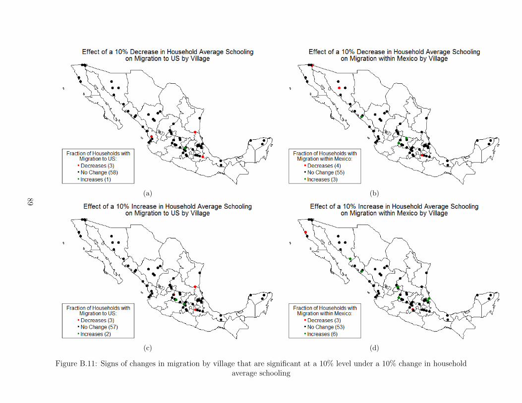
(a) (b)

(c) (d)

Figure B.11: Signs of changes in migration by village that are significant at a 10% level under a 10% change in householdaverage schooling

89

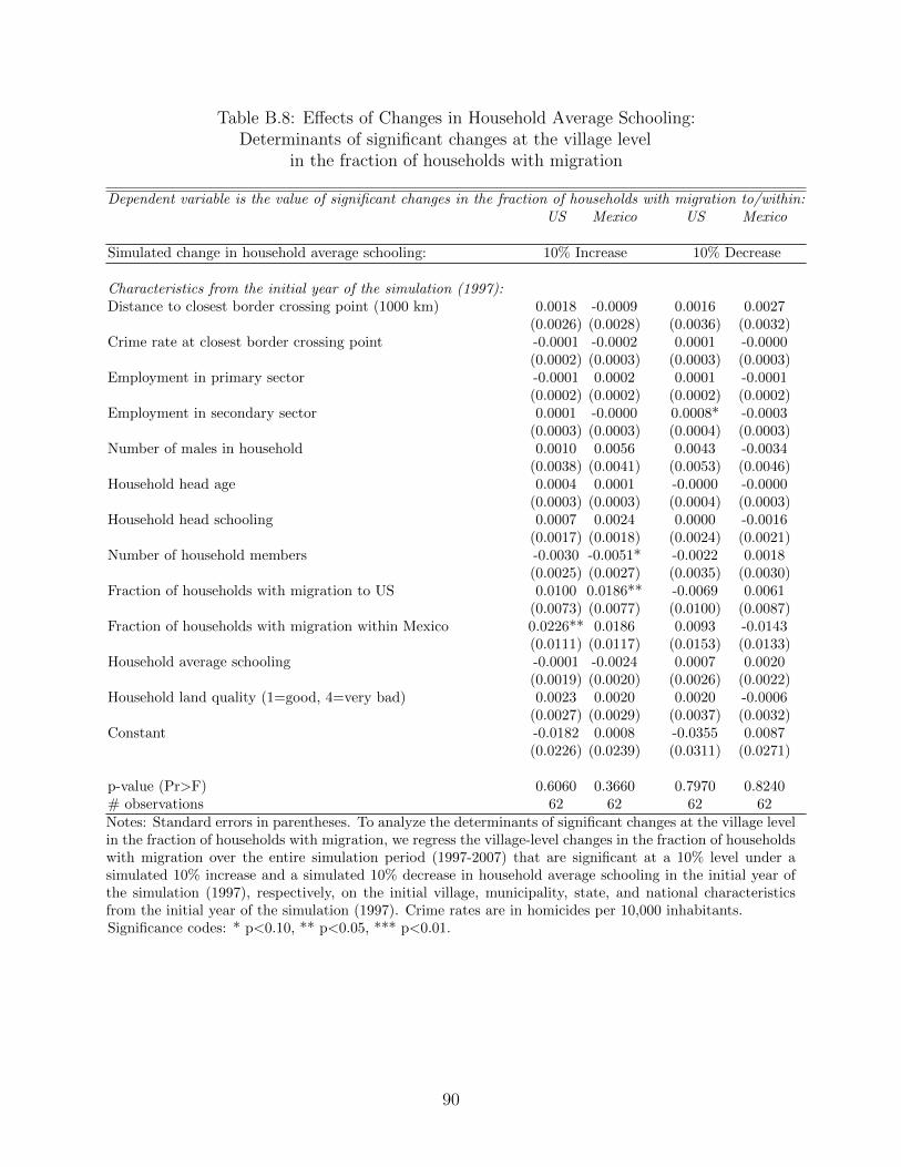
Table B.8: Effects of Changes in Household Average Schooling:Determinants of significant changes at the village level

in the fraction of households with migration

Dependent variable is the value of significant changes in the fraction of households with migration to/within:US Mexico US Mexico

Simulated change in household average schooling: 10% Increase 10% Decrease

Characteristics from the initial year of the simulation (1997):Distance to closest border crossing point (1000 km) 0.0018 -0.0009 0.0016 0.0027

(0.0026) (0.0028) (0.0036) (0.0032)Crime rate at closest border crossing point -0.0001 -0.0002 0.0001 -0.0000

(0.0002) (0.0003) (0.0003) (0.0003)Employment in primary sector -0.0001 0.0002 0.0001 -0.0001

(0.0002) (0.0002) (0.0002) (0.0002)Employment in secondary sector 0.0001 -0.0000 0.0008* -0.0003

(0.0003) (0.0003) (0.0004) (0.0003)Number of males in household 0.0010 0.0056 0.0043 -0.0034

(0.0038) (0.0041) (0.0053) (0.0046)Household head age 0.0004 0.0001 -0.0000 -0.0000

(0.0003) (0.0003) (0.0004) (0.0003)Household head schooling 0.0007 0.0024 0.0000 -0.0016

(0.0017) (0.0018) (0.0024) (0.0021)Number of household members -0.0030 -0.0051* -0.0022 0.0018

(0.0025) (0.0027) (0.0035) (0.0030)Fraction of households with migration to US 0.0100 0.0186** -0.0069 0.0061

(0.0073) (0.0077) (0.0100) (0.0087)Fraction of households with migration within Mexico 0.0226** 0.0186 0.0093 -0.0143

(0.0111) (0.0117) (0.0153) (0.0133)Household average schooling -0.0001 -0.0024 0.0007 0.0020

(0.0019) (0.0020) (0.0026) (0.0022)Household land quality (1=good, 4=very bad) 0.0023 0.0020 0.0020 -0.0006

(0.0027) (0.0029) (0.0037) (0.0032)Constant -0.0182 0.0008 -0.0355 0.0087

(0.0226) (0.0239) (0.0311) (0.0271)

p-value (Pr>F) 0.6060 0.3660 0.7970 0.8240# observations 62 62 62 62Notes: Standard errors in parentheses. To analyze the determinants of significant changes at the village levelin the fraction of households with migration, we regress the village-level changes in the fraction of householdswith migration over the entire simulation period (1997-2007) that are significant at a 10% level under asimulated 10% increase and a simulated 10% decrease in household average schooling in the initial year ofthe simulation (1997), respectively, on the initial village, municipality, state, and national characteristicsfrom the initial year of the simulation (1997). Crime rates are in homicides per 10,000 inhabitants.Significance codes: * p<0.10, ** p<0.05, *** p<0.01.

90

(a)

(b)

Figure B.12: Signs of changes in average welfare per household-year by village that aresignificant at a 10% level under a 10% change in household average schooling

91

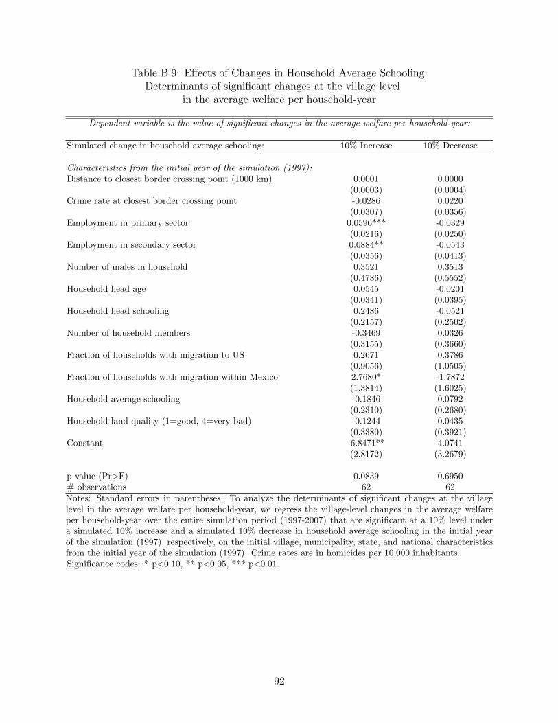
Table B.9: Effects of Changes in Household Average Schooling:Determinants of significant changes at the village level

in the average welfare per household-year

Dependent variable is the value of significant changes in the average welfare per household-year:

Simulated change in household average schooling: 10% Increase 10% Decrease

Characteristics from the initial year of the simulation (1997):Distance to closest border crossing point (1000 km) 0.0001 0.0000

(0.0003) (0.0004)Crime rate at closest border crossing point -0.0286 0.0220

(0.0307) (0.0356)Employment in primary sector 0.0596*** -0.0329

(0.0216) (0.0250)Employment in secondary sector 0.0884** -0.0543

(0.0356) (0.0413)Number of males in household 0.3521 0.3513

(0.4786) (0.5552)Household head age 0.0545 -0.0201

(0.0341) (0.0395)Household head schooling 0.2486 -0.0521

(0.2157) (0.2502)Number of household members -0.3469 0.0326

(0.3155) (0.3660)Fraction of households with migration to US 0.2671 0.3786

(0.9056) (1.0505)Fraction of households with migration within Mexico 2.7680* -1.7872

(1.3814) (1.6025)Household average schooling -0.1846 0.0792

(0.2310) (0.2680)Household land quality (1=good, 4=very bad) -0.1244 0.0435

(0.3380) (0.3921)Constant -6.8471** 4.0741

(2.8172) (3.2679)

p-value (Pr>F) 0.0839 0.6950# observations 62 62Notes: Standard errors in parentheses. To analyze the determinants of significant changes at the villagelevel in the average welfare per household-year, we regress the village-level changes in the average welfareper household-year over the entire simulation period (1997-2007) that are significant at a 10% level undera simulated 10% increase and a simulated 10% decrease in household average schooling in the initial yearof the simulation (1997), respectively, on the initial village, municipality, state, and national characteristicsfrom the initial year of the simulation (1997). Crime rates are in homicides per 10,000 inhabitants.Significance codes: * p<0.10, ** p<0.05, *** p<0.01.

92

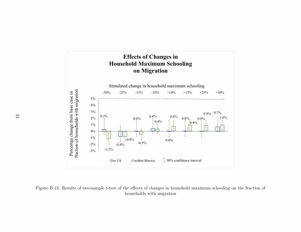
0.3%

-0.8%

0.0%0.4%

0.0%

0.0% 0.0%

0.7%

-1.2%

-0.8%-0.5%

0.4%0.8%

0.9%

0.9%1.0%

-3%

-2%

-1%

0%

1%

2%

3%

4%

5%

-50% -25% -15% -10% +10% +15% +25% +50%

Effects of Changes inHousehold Maximum Schooling

on Migration

to US within Mexico

Perc

entg

ech

ange

fro

m b

ase

case

in

frac

tion

of

hous

ehol

ds w

ith

mig

rati

on

Simulated change in household maximum schooling

90% confidence interval

Figure B.13: Results of two-sample t-test of the effects of changes in household maximum schooling on the fraction ofhouseholds with migration

93

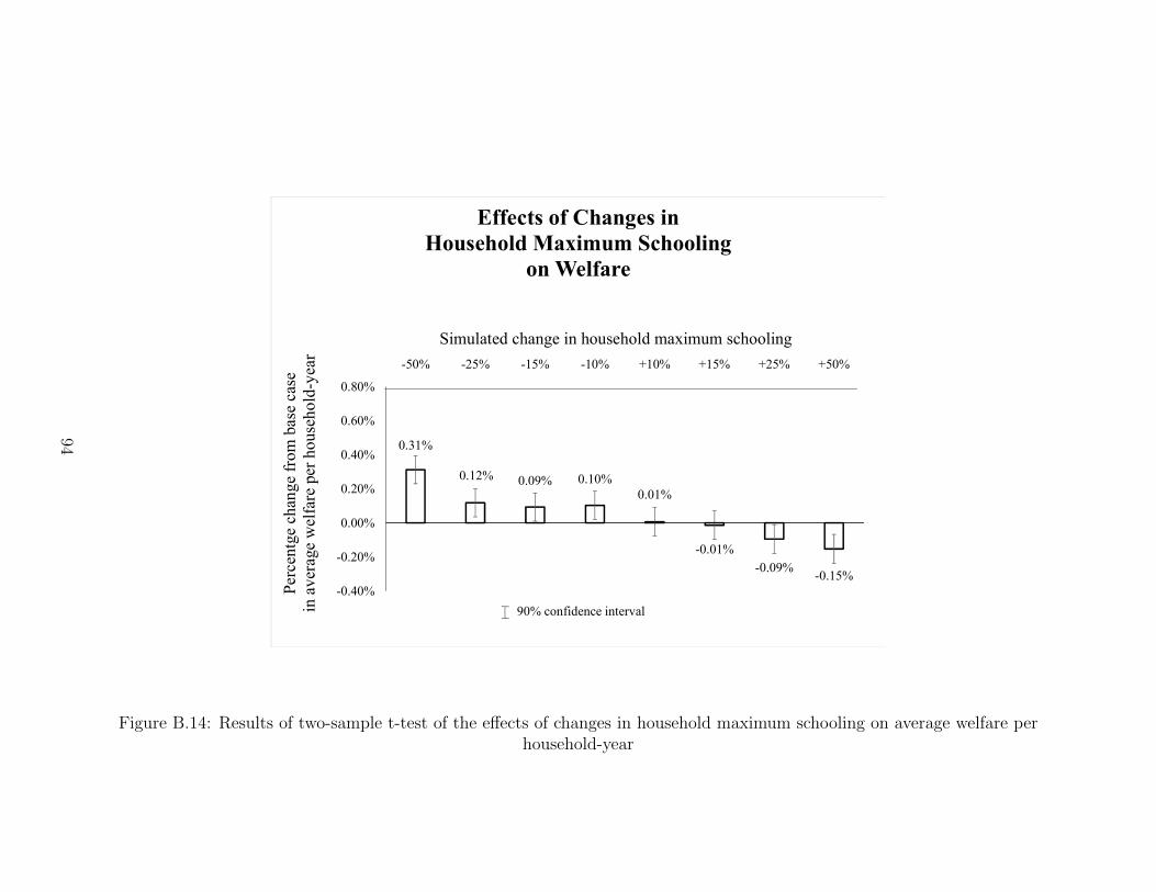
0.31%

0.12% 0.09% 0.10%0.01%

-0.01%

-0.09%-0.15%

-0.40%

-0.20%

0.00%

0.20%

0.40%

0.60%

0.80%

-50% -25% -15% -10% +10% +15% +25% +50%

Effects of Changes inHousehold Maximum Schooling

on WelfarePe

rcen

tge

chan

ge f

rom

bas

e ca

se

in a

vera

ge w

elfa

re p

er h

ouse

hold

-yea

r

Simulated change in household maximum schooling

90% confidence interval

Figure B.14: Results of two-sample t-test of the effects of changes in household maximum schooling on average welfare perhousehold-year

94

(a) (b)

(c) (d)

Figure B.15: Signs of changes in migration by village that are significant at a 10% level under a 10% change in householdmaximum schooling

95

Table B.10: Effects of Changes in Household Maximum Schooling:Determinants of significant changes at the village level

in the fraction of households with migration

Dependent variable is the value of significant changes in the fraction of households with migration to/within:US Mexico US Mexico

Simulated change in household max schooling: 10% Increase 10% Decrease

Characteristics from the initial year of the simulation (1997):Distance to closest border crossing point (1000 km) -0.0029 0.0024 -0.0016 0.0036

(0.0031) (0.0027) (0.0026) (0.0027)Crime rate at closest border crossing point 0.0001 -0.0001 -0.0000 -0.0002

(0.0003) (0.0003) (0.0002) (0.0002)Employment in primary sector -0.0005** 0.0004** -0.0002 0.0003*

(0.0002) (0.0002) (0.0002) (0.0002)Employment in secondary sector -0.0005 0.0001 -0.0001 0.0006**

(0.0003) (0.0003) (0.0003) (0.0003)Number of males in household -0.0069 0.0046 -0.0050 0.0028

(0.0045) (0.0039) (0.0038) (0.0039)Household head age 0.0004 -0.0001 0.0004 0.0002

(0.0003) (0.0003) (0.0003) (0.0003)Household head schooling 0.0011 -0.0033* 0.0004 -0.0000

(0.0020) (0.0018) (0.0017) (0.0017)Number of household members 0.0024 -0.0021 0.0000 -0.0027

(0.0030) (0.0026) (0.0025) (0.0025)Fraction of households with migration to US 0.0069 0.0009 0.0086 0.0033

(0.0086) (0.0074) (0.0072) (0.0073)Fraction of households with migration within Mexico 0.0187 -0.0217* 0.0269** -0.0051

(0.0131) (0.0114) (0.0110) (0.0111)Household average schooling -0.0012 0.0036* -0.0010 -0.0003

(0.0022) (0.0019) (0.0018) (0.0019)Household land quality (1=good, 4=very bad) -0.0004 -0.0010 -0.0001 -0.0005

(0.0032) (0.0028) (0.0027) (0.0027)Constant 0.0115 -0.0053 0.0067 -0.0171

(0.0267) (0.0232) (0.0225) (0.0227)

p-value (Pr>F) 0.2710 0.0609 0.1430 0.6210# observations 62 62 62 62Notes: Standard errors in parentheses. To analyze the determinants of significant changes at the village levelin the fraction of households with migration, we regress the village-level changes in the fraction of householdswith migration over the entire simulation period (1997-2007) that are significant at a 10% level under asimulated 10% increase and a simulated 10% decrease in household maximum schooling in the initial yearof the simulation (1997), respectively, on the initial village, municipality, state, and national characteristicsfrom the initial year of the simulation (1997). Crime rates are in homicides per 10,000 inhabitants.Significance codes: * p<0.10, ** p<0.05, *** p<0.01.

96

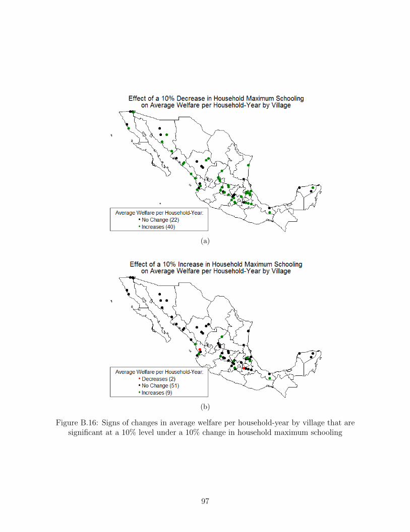
(a)

(b)

Figure B.16: Signs of changes in average welfare per household-year by village that aresignificant at a 10% level under a 10% change in household maximum schooling

97

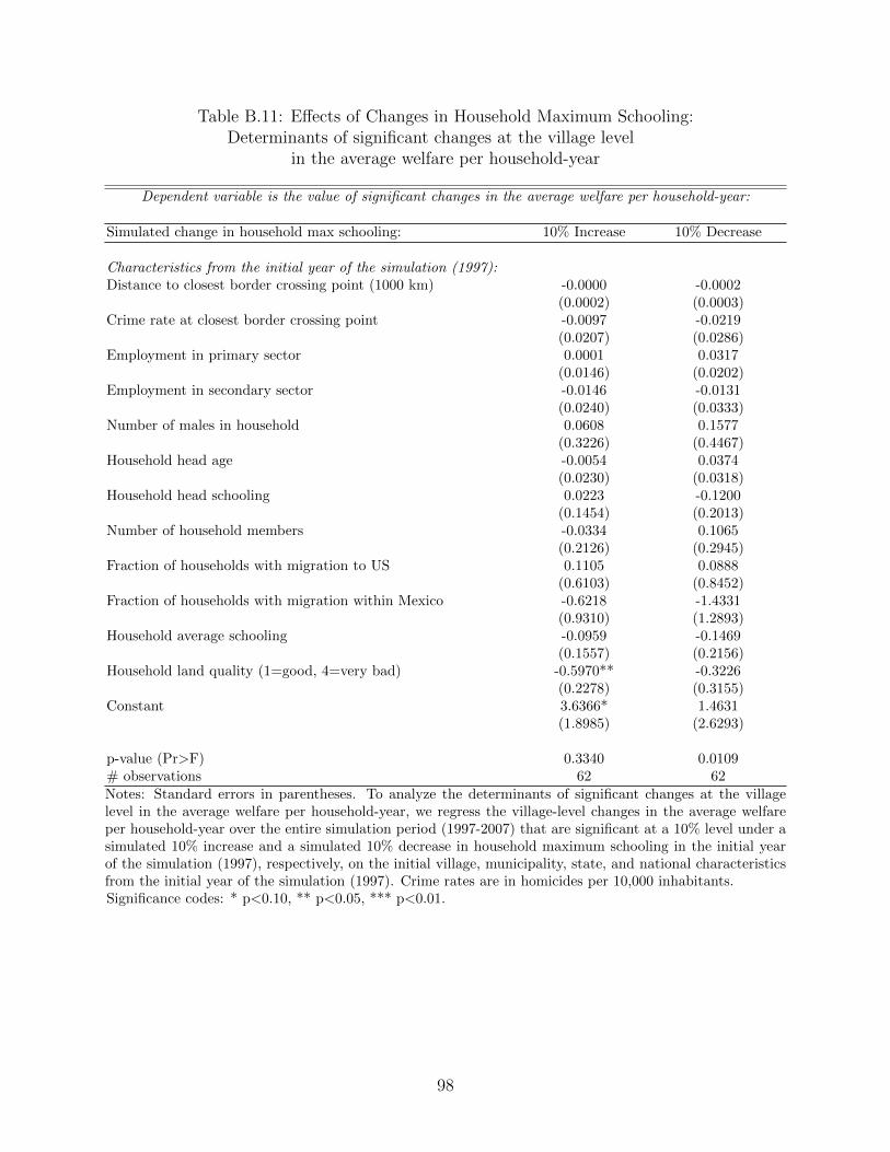
Table B.11: Effects of Changes in Household Maximum Schooling:Determinants of significant changes at the village level

in the average welfare per household-year

Dependent variable is the value of significant changes in the average welfare per household-year:

Simulated change in household max schooling: 10% Increase 10% Decrease

Characteristics from the initial year of the simulation (1997):Distance to closest border crossing point (1000 km) -0.0000 -0.0002

(0.0002) (0.0003)Crime rate at closest border crossing point -0.0097 -0.0219

(0.0207) (0.0286)Employment in primary sector 0.0001 0.0317

(0.0146) (0.0202)Employment in secondary sector -0.0146 -0.0131

(0.0240) (0.0333)Number of males in household 0.0608 0.1577

(0.3226) (0.4467)Household head age -0.0054 0.0374

(0.0230) (0.0318)Household head schooling 0.0223 -0.1200

(0.1454) (0.2013)Number of household members -0.0334 0.1065

(0.2126) (0.2945)Fraction of households with migration to US 0.1105 0.0888

(0.6103) (0.8452)Fraction of households with migration within Mexico -0.6218 -1.4331

(0.9310) (1.2893)Household average schooling -0.0959 -0.1469

(0.1557) (0.2156)Household land quality (1=good, 4=very bad) -0.5970** -0.3226

(0.2278) (0.3155)Constant 3.6366* 1.4631

(1.8985) (2.6293)

p-value (Pr>F) 0.3340 0.0109# observations 62 62Notes: Standard errors in parentheses. To analyze the determinants of significant changes at the villagelevel in the average welfare per household-year, we regress the village-level changes in the average welfareper household-year over the entire simulation period (1997-2007) that are significant at a 10% level under asimulated 10% increase and a simulated 10% decrease in household maximum schooling in the initial yearof the simulation (1997), respectively, on the initial village, municipality, state, and national characteristicsfrom the initial year of the simulation (1997). Crime rates are in homicides per 10,000 inhabitants.Significance codes: * p<0.10, ** p<0.05, *** p<0.01.

98

0.1%0.8%

0.0%

-0.4%

0.2% 0.2% 0.1%

0.7%

-0.7%-0.2%

0.0%

-0.2%

0.7%

0.0%

0.3%0.8%

-2%

-1%

0%

1%

2%

3%

4%

5%

-50% -25% -15% -10% +10% +15% +25% +50%

Effects of Changes inCrime Rate at the Border

on Migration

to US within Mexico

Perc

entg

ech

ange

fro

m b

ase

case

in

frac

tion

of

hous

ehol

ds w

ith

mig

rati

on

Simulated change in crime rate

90% confidence interval

Figure B.17: Results of two-sample t-test of the effects of changes in crime rate at the border on the fraction of householdswith migration

99

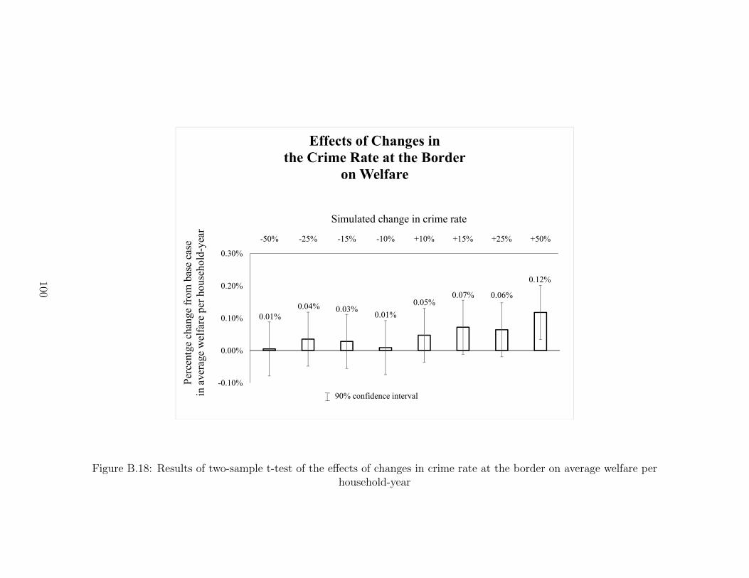
0.01%0.04% 0.03%

0.01%

0.05%0.07% 0.06%

0.12%

-0.10%

0.00%

0.10%

0.20%

0.30%

-50% -25% -15% -10% +10% +15% +25% +50%

Effects of Changes inthe Crime Rate at the Border

on WelfareP

erce

ntge

chan

ge f

rom

bas

e ca

se

in a

vera

ge w

elfa

re p

er h

ouse

hold

-yea

r

Simulated change in crime rate

90% confidence interval

Figure B.18: Results of two-sample t-test of the effects of changes in crime rate at the border on average welfare perhousehold-year

100

(a) (b)

(c) (d)

Figure B.19: Signs of changes in migration by village that are significant at a 10% level under a 10% change in crime rate atthe border

101

Table B.12: Effects of Changes in Crime Rate at the Border:Determinants of significant changes at the village level

in the fraction of households with migration

Dependent variable is the value of significant changes in the fraction of households with migration to/within:US Mexico US Mexico

Simulated change in crime rate: 10% Increase 10% Decrease

Characteristics from the initial year of the simulation (1997):Distance to closest border crossing point (1000 km) 0.0005 0.0025 -0.0001 0.0008

(0.0038) (0.0052) (0.0021) (0.0046)Crime rate at closest border crossing point 0.0001 0.0000 -0.0001 0.0000

(0.0004) (0.0005) (0.0002) (0.0004)Employment in primary sector -0.0001 -0.0003 0.0000 -0.0004

(0.0002) (0.0003) (0.0001) (0.0003)Employment in secondary sector 0.0004 -0.0012** -0.0000 -0.0010*

(0.0004) (0.0006) (0.0002) (0.0005)Number of males in household -0.0049 0.0110 -0.0058* 0.0111

(0.0055) (0.0076) (0.0030) (0.0067)Household head age 0.0003 -0.0003 0.0002 -0.0003

(0.0004) (0.0005) (0.0002) (0.0005)Household head schooling 0.0004 0.0010 -0.0017 0.0027

(0.0025) (0.0034) (0.0014) (0.0030)Number of household members 0.0010 -0.0027 0.0015 -0.0053

(0.0036) (0.0050) (0.0020) (0.0044)Fraction of households with migration to US -0.0050 0.0009 -0.0020 0.0219*

(0.0104) (0.0143) (0.0057) (0.0126)Fraction of households with migration within Mexico 0.0286* -0.0412* 0.0068 -0.0048

(0.0158) (0.0219) (0.0087) (0.0193)Household average schooling -0.0004 -0.0029 0.0018 -0.0033

(0.0026) (0.0037) (0.0015) (0.0032)Household land quality (1=good, 4=very bad) 0.0025 -0.0119** 0.0012 -0.0063

(0.0039) (0.0054) (0.0021) (0.0047)Constant -0.0264 0.0952** -0.0100 0.0747*

(0.0322) (0.0446) (0.0178) (0.0393)

p-value (Pr>F) 0.4400 0.1210 0.4930 0.3900# observations 62 62 62 62Notes: Standard errors in parentheses. To analyze the determinants of significant changes at the villagelevel in the fraction of households with migration, we regress the village-level changes in the fraction ofhouseholds with migration over the entire simulation period (1997-2007) that are significant at a 10% levelunder a simulated 10% increase and a simulated 10% decrease in crime rate at the border in the initial yearof the simulation (1997), respectively, on the initial village, municipality, state, and national characteristicsfrom the initial year of the simulation (1997). Crime rates are in homicides per 10,000 inhabitants.Significance codes: * p<0.10, ** p<0.05, *** p<0.01.

102

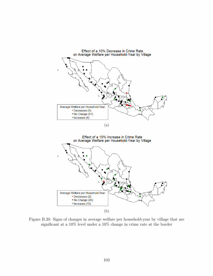
(a)

(b)

Figure B.20: Signs of changes in average welfare per household-year by village that aresignificant at a 10% level under a 10% change in crime rate at the border

103

Table B.13: Effects of Changes in Crime Rate at the Border:Determinants of significant changes at the village level

in the average welfare per household-year

Dependent variable is the value of significant changes in the average welfare per household-year:

Simulated change in crime rate: 10% Increase 10% Decrease

Characteristics from the initial year of the simulation (1997):Distance to closest border crossing point (1000 km) -0.0001 0.0002

(0.0004) (0.0002)Crime rate at closest border crossing point -0.0063 -0.0050

(0.0329) (0.0230)Employment in primary sector -0.0024 -0.0039

(0.0232) (0.0162)Employment in secondary sector -0.0291 -0.0142

(0.0382) (0.0267)Number of males in household 0.5125 -0.0046

(0.5132) (0.3583)Household head age -0.0012 0.0073

(0.0366) (0.0255)Household head schooling 0.0787 0.0447

(0.2313) (0.1615)Number of household members -0.1508 0.0368

(0.3383) (0.2362)Fraction of households with migration to US 0.0172 -0.1842

(0.9711) (0.6780)Fraction of households with migration within Mexico -1.3377 -1.0705

(1.4813) (1.0342)Household average schooling -0.2942 -0.0912

(0.2477) (0.1729)Household land quality (1=good, 4=very bad) -0.7625** -0.0564

(0.3625) (0.2531)Constant 5.1434* 0.6506

(3.0208) (2.1090)

p-value (Pr>F) 0.2450 0.9940# observations 62 62Notes: Standard errors in parentheses. To analyze the determinants of significant changes at the villagelevel in the average welfare per household-year, we regress the village-level changes in the average welfareper household-year over the entire simulation period (1997-2007) that are significant at a 10% level under asimulated 10% increase and a simulated 10% decrease in crime rate at the border in the initial year of thesimulation (1997), respectively, on the initial village, municipality, state, and national characteristics fromthe initial year of the simulation (1997). Crime rates are in homicides per 10,000 inhabitants.Significance codes: * p<0.10, ** p<0.05, *** p<0.01.

104

0.2%0.6%

0.2%2.3%

0.1%0.8% 0.5%

0.9%

-0.6%-0.2%

0.7% 0.7%

-0.1%

0.3% 0.0%0.5%

-2%

-1%

0%

1%

2%

3%

4%

5%

6%

7%

-50% -25% -15% -10% +10% +15% +25% +50%

Effects of Changesin Precipitationon Migration

to US within Mexico

Perc

entg

ech

ange

fro

m b

ase

case

in

frac

tion

of

hous

ehol

ds w

ith

mig

rati

on

Simulated change in precipitation

90% confidence interval

Figure B.21: Results of two-sample t-test of the effects of changes in precipitation on the fraction of households with migration

105

(a) (b)

(c) (d)

Figure B.22: Signs of changes in migration by village that are significant at a 10% level under a 10% change in precipitation

106

Table B.14: Effects of Changes in Precipitation:Determinants of significant changes at the village level

in the fraction of households with migration

Dependent variable is the value of significant changes in the fraction of households with migration to/within:US Mexico US Mexico

Simulated change in precipitation: 10% Increase 10% Decrease

Characteristics from the initial year of the simulation (1997):Distance to closest border crossing point (1000 km) -0.0000 0.0022 -0.0013 0.0008

(0.0024) (0.0045) (0.0046) (0.0034)Crime rate at closest border crossing point 0.0001 -0.0001 -0.0000 -0.0002

(0.0002) (0.0004) (0.0004) (0.0003)Employment in primary sector 0.0001 -0.0000 0.0002 0.0002

(0.0002) (0.0003) (0.0003) (0.0002)Employment in secondary sector -0.0001 -0.0009* 0.0003 -0.0000

(0.0003) (0.0005) (0.0005) (0.0004)Number of males in household -0.0040 0.0111* 0.0059 -0.0008

(0.0034) (0.0066) (0.0066) (0.0049)Household head age 0.0003 -0.0001 0.0001 0.0002

(0.0002) (0.0005) (0.0005) (0.0003)Household head schooling -0.0024 0.0023 0.0030 0.0004

(0.0016) (0.0030) (0.0030) (0.0022)Number of household members 0.0010 -0.0060 -0.0047 -0.0002

(0.0023) (0.0043) (0.0044) (0.0032)Fraction of households with migration to US -0.0108 0.0217* 0.0058 0.0085

(0.0065) (0.0124) (0.0126) (0.0093)Fraction of households with migration within Mexico 0.0008 -0.0078 0.0257 -0.0157

(0.0099) (0.0189) (0.0192) (0.0142)Household average schooling 0.0030* -0.0044 -0.0022 -0.0004

(0.0017) (0.0032) (0.0032) (0.0024)Household land quality (1=good, 4=very bad) 0.0014 -0.0068 -0.0013 0.0012

(0.0024) (0.0046) (0.0047) (0.0035)Constant -0.0215 0.0705* -0.0032 -0.0073

(0.0203) (0.0386) (0.0391) (0.0289)

p-value (Pr>F) 0.3010 0.1190 0.9300 0.7150# observations 62 62 62 62Notes: Standard errors in parentheses. To analyze the determinants of significant changes at the villagelevel in the fraction of households with migration, we regress the village-level changes in the fraction ofhouseholds with migration over the entire simulation period (1997-2007) that are significant at a 10% levelunder a simulated 10% increase and a simulated 10% decrease in precipitation in the initial year of thesimulation (1997), respectively, on the initial village, municipality, state, and national characteristics fromthe initial year of the simulation (1997). Crime rates are in homicides per 10,000 inhabitants.Significance codes: * p<0.10, ** p<0.05, *** p<0.01.

107

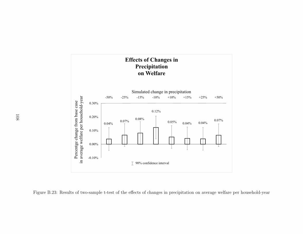
0.04%0.07%

0.08%

0.12%

0.05% 0.04% 0.04%0.07%

-0.10%

0.00%

0.10%

0.20%

0.30%

-50% -25% -15% -10% +10% +15% +25% +50%

Effects of Changes inPrecipitationon Welfare

Per

cent

gech

ange

fro

m b

ase

case

in

ave

rage

wel

fare

per

hou

seho

ld-y

ear

Simulated change in precipitation

90% confidence interval

Figure B.23: Results of two-sample t-test of the effects of changes in precipitation on average welfare per household-year

108

(a)

(b)

Figure B.24: Signs of changes in average welfare per household-year by village that aresignificant at a 10% level under a 10% change in precipitation

109

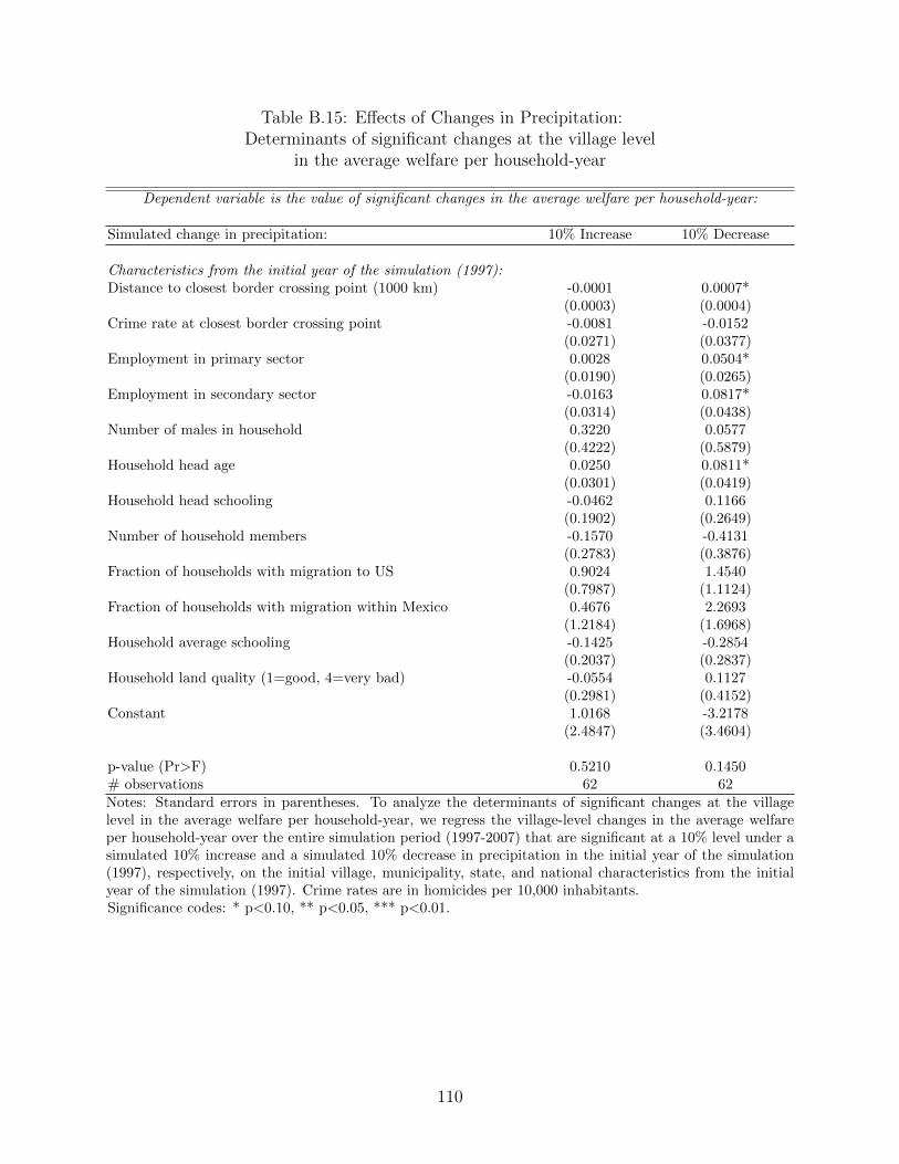
Table B.15: Effects of Changes in Precipitation:Determinants of significant changes at the village level

in the average welfare per household-year

Dependent variable is the value of significant changes in the average welfare per household-year:

Simulated change in precipitation: 10% Increase 10% Decrease

Characteristics from the initial year of the simulation (1997):Distance to closest border crossing point (1000 km) -0.0001 0.0007*

(0.0003) (0.0004)Crime rate at closest border crossing point -0.0081 -0.0152

(0.0271) (0.0377)Employment in primary sector 0.0028 0.0504*

(0.0190) (0.0265)Employment in secondary sector -0.0163 0.0817*

(0.0314) (0.0438)Number of males in household 0.3220 0.0577

(0.4222) (0.5879)Household head age 0.0250 0.0811*

(0.0301) (0.0419)Household head schooling -0.0462 0.1166

(0.1902) (0.2649)Number of household members -0.1570 -0.4131

(0.2783) (0.3876)Fraction of households with migration to US 0.9024 1.4540

(0.7987) (1.1124)Fraction of households with migration within Mexico 0.4676 2.2693

(1.2184) (1.6968)Household average schooling -0.1425 -0.2854

(0.2037) (0.2837)Household land quality (1=good, 4=very bad) -0.0554 0.1127

(0.2981) (0.4152)Constant 1.0168 -3.2178

(2.4847) (3.4604)

p-value (Pr>F) 0.5210 0.1450# observations 62 62Notes: Standard errors in parentheses. To analyze the determinants of significant changes at the villagelevel in the average welfare per household-year, we regress the village-level changes in the average welfareper household-year over the entire simulation period (1997-2007) that are significant at a 10% level under asimulated 10% increase and a simulated 10% decrease in precipitation in the initial year of the simulation(1997), respectively, on the initial village, municipality, state, and national characteristics from the initialyear of the simulation (1997). Crime rates are in homicides per 10,000 inhabitants.Significance codes: * p<0.10, ** p<0.05, *** p<0.01.

110

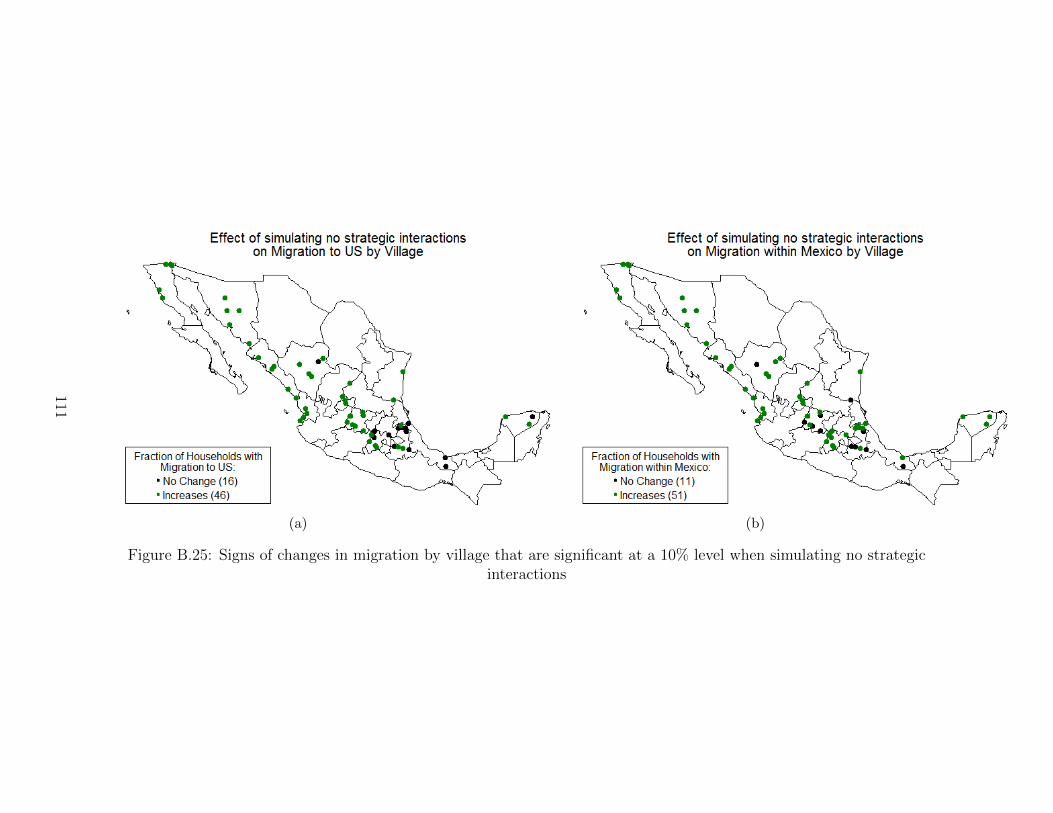
(a) (b)

Figure B.25: Signs of changes in migration by village that are significant at a 10% level when simulating no strategicinteractions

111

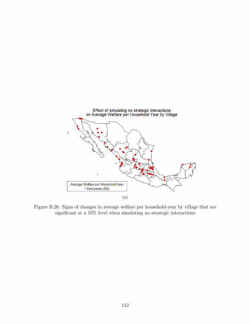
(a)

Figure B.26: Signs of changes in average welfare per household-year by village that aresignificant at a 10% level when simulating no strategic interactions

112

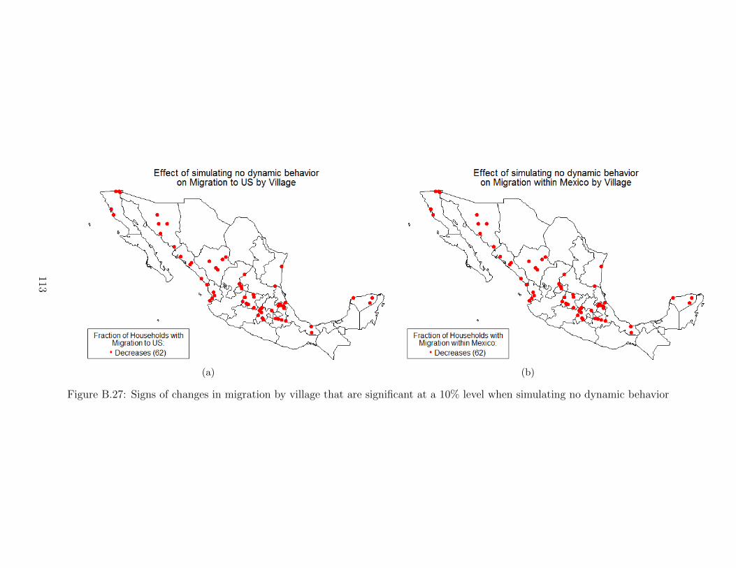
(a) (b)

Figure B.27: Signs of changes in migration by village that are significant at a 10% level when simulating no dynamic behavior

113

(a)

Figure B.28: Signs of changes in average welfare per household-year by village that aresignificant at a 10% level when simulating no dynamic behavior

114

-1.28% -1.26% -1.27% -1.28%-1.60%

-1.40%

-1.20%

-1.00%

-0.80%

-0.60%

-0.40%

-0.20%

0.00%

0.20%

50% 75% 85% 90%

Effects of a Cap on Migration to the USand No Strategic Interactions

on WelfareP

erce

ntge

chan

ge f

rom

bas

e ca

se

in a

vera

ge w

elfa

re p

er h

ouse

hold

-yea

rCap as % of base case migration that is denied migration to the US

90% confidence interval

Figure B.29: Results of two-sample t-test of the effects of a cap on migration to US with no strategic interactions on averagewelfare per household-year

115

(a) (b)

Figure B.30: Signs of changes in migration by village that are significant at a 10% level under a cap of 90% of base casemigration and no strategic interactions

116

(a)

Figure B.31: Signs of changes in average welfare per household-year by village that aresignificant at a 10% level under a cap of 90% of base case migration and no strategic

interactions

117

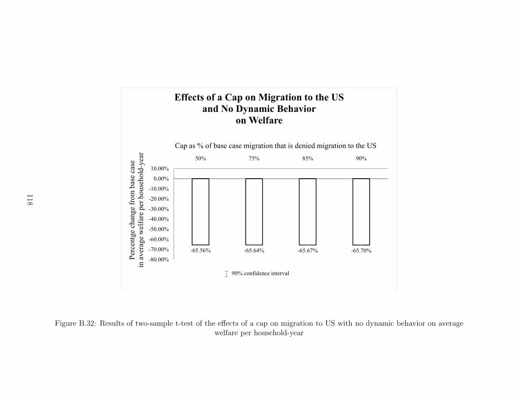
-65.56% -65.64% -65.67% -65.70%

-80.00%

-70.00%

-60.00%

-50.00%

-40.00%

-30.00%

-20.00%

-10.00%

0.00%

10.00%

50% 75% 85% 90%

Effects of a Cap on Migration to the USand No Dynamic Behavior

on WelfareP

erce

ntge

chan

ge f

rom

bas

e ca

se

in a

vera

ge w

elfa

re p

er h

ouse

hold

-yea

rCap as % of base case migration that is denied migration to the US

90% confidence interval

Figure B.32: Results of two-sample t-test of the effects of a cap on migration to US with no dynamic behavior on averagewelfare per household-year

118

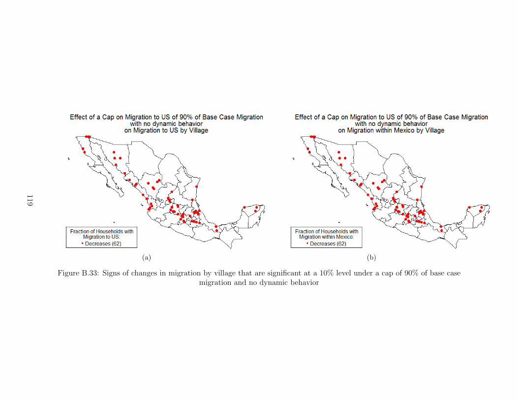
(a) (b)

Figure B.33: Signs of changes in migration by village that are significant at a 10% level under a cap of 90% of base casemigration and no dynamic behavior

119

(a)

Figure B.34: Signs of changes in average welfare per household-year by village that aresignificant at a 10% level under a cap of 90% of base case migration and no dynamic

behavior

120