THE DIRECTED FOREST

COMPLEX OF CAYLEY GRAPHS

by

Kennedy Courtney

A thesis

submitted in partial fulfillment

of the requirements for the degree of

Master of Science in Mathematics

Boise State University

May 2020

© 2020Kennedy Courtney

ALL RIGHTS RESERVED

BOISE STATE UNIVERSITY GRADUATE COLLEGE

DEFENSE COMMITTEE AND FINAL READING APPROVALS

of the thesis submitted by

Kennedy Courtney

Thesis Title: The Directed Forest Complex of Cayley Graphs

Date of Final Oral Examination: 6 March 2020

The following individuals read and discussed the thesis submitted by student KennedyCourtney, and they evaluated her presentation and response to questions during thefinal oral examination. They found that the student passed the final oral examination.

Jens Harlander, Ph.D. Chair, Supervisory Committee

Uwe Kaiser, Ph.D. Member, Supervisory Committee

Zachariah Teitler, Ph.D. Member, Supervisory Committee

The final reading approval of the thesis was granted by Jens Harlander, Ph.D., Chairof the Supervisory Committee. The thesis was approved by the Graduate College.

To all those who struggle through math, but persist.

iv

ACKNOWLEDGMENTS

I would like to express my deepest appreciation to my advisor, Dr. Jens Harlander,

whose vision and patience gave rise to an excellent research experience. I would also

like to acknowledge my committee for their sharp eyes and sharp minds in the editing

process of this thesis.

Thank you to my family for always believing and investing in me, my friends from

Portland for giving long distance support, my community here at Boise State for

sharing the joys and frustrations of graduate school with me, and my partner, Rahul,

for his endless love and support throughout the process.

In addition, I would like to thank Dr. Christopher R. Lee, without whose guidance

I would not have pursued graduate school. Thank you for meeting me where I was at

without judgement, sharing opportunities to learn, and being a model of vulnerability.

Your mentorship is invaluable element in my evolution, and I am wholly grateful for it.

v

ABSTRACT

Let Γ be a directed graph. The directed forest complex, DF(Γ), is a simplicial

complex whose vertices are the edges of Γ and whose simplices are sets of edges that

form a directed forest in Γ. We study the directed forest complex of Cayley graphs of

finite groups. The homology of DF(Γ) contains information about the graph, Γ and

about the group, G. The ultimate goal is to classify DF(Γ) up to homotopy, compute

its homology, and interpret the findings in terms of properties of Γ. In this thesis, we

present progress made toward this goal.

vi

TABLE OF CONTENTS

DEDICATION . . . . . . . . . . . . . . . . . . . . . . . . . . . . . . . . . . . . . . . . . . . . . . iv

ACKNOWLEDGMENTS . . . . . . . . . . . . . . . . . . . . . . . . . . . . . . . . . . . . . v

Abstract . . . . . . . . . . . . . . . . . . . . . . . . . . . . . . . . . . . . . . . . . . . . . . . . . . . vi

List of Figures . . . . . . . . . . . . . . . . . . . . . . . . . . . . . . . . . . . . . . . . . . . . . . viii

1 Introduction . . . . . . . . . . . . . . . . . . . . . . . . . . . . . . . . . . . . . . . . . . . . . . 1

2 Simplicial Complexes . . . . . . . . . . . . . . . . . . . . . . . . . . . . . . . . . . . . . . 4

3 Survey of Engstrom . . . . . . . . . . . . . . . . . . . . . . . . . . . . . . . . . . . . . . . 10

4 The Directed Forest Complex of a Cayley Graph . . . . . . . . . . . . . . . 22

4.1 Cayley graphs . . . . . . . . . . . . . . . . . . . . . . . . . . . . . . . . . . . . . . . . . . . . . 22

4.2 The question of purity . . . . . . . . . . . . . . . . . . . . . . . . . . . . . . . . . . . . . . 27

4.3 Actions and stabilizers . . . . . . . . . . . . . . . . . . . . . . . . . . . . . . . . . . . . . . 29

4.4 Simple connectivity . . . . . . . . . . . . . . . . . . . . . . . . . . . . . . . . . . . . . . . . 32

4.5 A fundamental domain . . . . . . . . . . . . . . . . . . . . . . . . . . . . . . . . . . . . . . 33

Bibliography . . . . . . . . . . . . . . . . . . . . . . . . . . . . . . . . . . . . . . . . . . . . . . . . 42

vii

LIST OF FIGURES

2.1 A geometric realization of the simplicial complex ∆ . . . . . . . . . . . . . . . . 5

2.2 A non-example of the geometric realization of a simplicial complex. . . . 6

2.3 1-dimensional, 2-dimensional, and 3-dimensional pure, shellable com-

plexes. . . . . . . . . . . . . . . . . . . . . . . . . . . . . . . . . . . . . . . . . . . . . . . . . . . . 7

2.4 A 1-dimensional connected simplicial complex with a shelling order. . . . 7

2.5 Caption . . . . . . . . . . . . . . . . . . . . . . . . . . . . . . . . . . . . . . . . . . . . . . . . . 8

3.1 An example of a directed forest. . . . . . . . . . . . . . . . . . . . . . . . . . . . . . . . 11

3.2 A directed graph. . . . . . . . . . . . . . . . . . . . . . . . . . . . . . . . . . . . . . . . . . . 12

3.3 The facets of DF(Γ). . . . . . . . . . . . . . . . . . . . . . . . . . . . . . . . . . . . . . . . . 12

3.4 The facets of DF{1,4}(Γ) . . . . . . . . . . . . . . . . . . . . . . . . . . . . . . . . . . . . . 12

3.5 The construction for DF{1,4}(Γ) in Example 3.0.1. . . . . . . . . . . . . . . . . . 14

3.6 The facet F = T1∪T2∪ · · · ∪Tn ∈ DF(Γ) and ri, the root of Ti, for every i19

3.7 Subcase 1. . . . . . . . . . . . . . . . . . . . . . . . . . . . . . . . . . . . . . . . . . . . . . . . . 20

3.8 Subcase 2. . . . . . . . . . . . . . . . . . . . . . . . . . . . . . . . . . . . . . . . . . . . . . . . . 20

3.9 Subcase 3. . . . . . . . . . . . . . . . . . . . . . . . . . . . . . . . . . . . . . . . . . . . . . . . . 21

4.1 General edge in a Cayley graph . . . . . . . . . . . . . . . . . . . . . . . . . . . . . . . 23

4.2 Γ = Γ(D3, {a, b}) . . . . . . . . . . . . . . . . . . . . . . . . . . . . . . . . . . . . . . . . . . 23

4.3 Γ = Γ(Z3 × Z3, {x, y}) . . . . . . . . . . . . . . . . . . . . . . . . . . . . . . . . . . . . . . 23

4.4 Cayley graph Γ(Z4). . . . . . . . . . . . . . . . . . . . . . . . . . . . . . . . . . . . . . . . . 25

viii

4.5 Top dimensional forests of DF(Z4). . . . . . . . . . . . . . . . . . . . . . . . . . . . . 25

4.6 The geometric realization of DF(Z4). . . . . . . . . . . . . . . . . . . . . . . . . . . . 26

4.7 The Cayley graph of D3 = 〈a, b | a2, b2, (ab)3〉. . . . . . . . . . . . . . . . . . . . . 29

4.8 Γ, the Cayley graph for G = Z2 × Z2 = 〈x, y|x2, y2, (xy)2〉 . . . . . . . . . . . 36

4.9 DFxy(Γ) DFy(Γ) DF1(Γ), DFx(Γ) . . . . . . . . . . . . . . . . . . . . . . . . . . . . . . 36

4.10 Some identifications made on the setDFxy(Γ) DFy(Γ) DF1(Γ), DFx(Γ). 37

4.11 The capping forests. . . . . . . . . . . . . . . . . . . . . . . . . . . . . . . . . . . . . . . . . 37

ix

1

Chapter 1

INTRODUCTION

One defines a directed tree as a directed graph that contains a vertex r (a root)

so that every other vertex v can be reached by a unique directed path from r to v.

A directed forest is a disjoint union of directed trees. Given a directed graph Γ, the

directed forest complex DF(Γ) (a simplicial complex) is defined in the following way:

the vertices of DF(Γ) are the edges of Γ, and a set of edges of Γ is a simplex of DF(Γ)

if the edges form a directed forest in Γ. The idea of a directed forest complex is due

to Richard Stanley (see Koslov [7]). The homology of DF(Γ) contains information

about the graph, for example every directed Hamiltonian cycle in Γ gives rise to a

top dimensional homology element. So the homology can “see” Hamiltonian cycles.

In this thesis, we study the directed forest complex of a Cayley graph Γ coming

from a finite group. We note that the question of whether Cayley graphs contain

Hamiltonian paths or cycles is a long standing open problem. See Curran-Gallian [4]

and also Pak-Radoicic [8]. The starting point of this thesis is a result of Engstrom

[5] that says that if Γ is an acyclic graph (and hence unlike a Cayley graph), that is

a directed graph that does not contain directed cycles, then DF(Γ) is shellable, see

definition 2.0.2. In particular DF(Γ) has the homotopy type of a wedge of spheres

(in various dimensions). Part of this thesis is a careful reworking of Engstroms result.

Here is a summary of our main results. We show that if Γ is a Cayley graph of

2

a group G then DF(Γ) might or might not be pure (i.e. all maximal simplices have

the same dimension). In either case we find that its dimension is |G| − 2. If |G| ≥ 16

then DF(Γ) is simply connected. Using a computer, we compute the homology of

some examples. One way to understand the homotopy type of DF(Γ) is by explicitely

constructing a shelling order. A daunting task. Another route is to construct a

good cover. In case DF(Γ) is pure we produce a fundamental domain DF1(Γ) for the

action of G on DF(Γ) (induced by the action of G on the Cayley graph Γ) and show

(using Engstrom [5]) that DF1(Γ) is shellable and contractible. This yields a nice

decomposition

DF(Γ) =⋃g∈G

DFg(Γ)

where each translate gDF1(Γ) = DFg(Γ) is shellable and contractible. We tried to

use this union to compute the homology of DF(Γ) using the Mayer-Vietoris spectral

sequence. This entails understanding the nerve of union on one hand, and intersec-

tions of the union members on the other hand (in order to understand the coefficient

system). We had success with the first part, but could not finish the second. We

proved that if Γ contains a Hamiltonian cycle, then the nerve is ∂∆(G), the boundary

of the full simplex on vertex set G. Topologically this is a sphere of dimension |G|−2.

Future goals are:

1. Understand purity of DF(Γ).

2. Understand shellability of DF(Γ).

3. Complete the computation of the homology of DF(Γ) for Cayley graphs in case

DF(Γ) is pure; the major part here is to understand how the DFg(Γ) intersect.

3

4. Interpret the homology in terms of properties of Γ and G. Is there a way

to decide which top-dimensional homology elements of H∗(DF(Γ)) come from

Hamiltonian cycles?

We have tried to make this thesis as self contained as possible. A good standard

reference for all matters concerning combinatorial topology is Koslov [6]. Background

on graph theory can be found in Bollobas [2].

4

Chapter 2

SIMPLICIAL COMPLEXES

Because the directed forest complex is a simplicial complex, we first define the

notion of a simplicial complex.

Definition 2.0.1. An (abstract) simplicial complex, ∆, on set of vertices, V , is a set

of finite subsets of V , generally called faces, which has the following property:

• If σ ∈ ∆ and τ ⊆ σ, then τ ∈ ∆.

Maximal faces in a simplicial complex are called facets. If σ = {v0, ..., vk} is a face

then the dimension of σ is k. The dimension of a simplicial complex ∆ is the maximal

dimension that occurs as the dimension of a facet.

Example 2.0.1. It is generally true that the set of facets determines the simpli-

cial complex. Let V = {a, b, c, d, e, f, g, h, i, j, k, l,m, n, o, p, q, r} and let ∆ be the

simplicial complex whose set of facets is

{{a, b, c, d}, {d, e, f}, {e, f, g}, {f, h, k}, {h, j}, {i, j},

{i, h}, {k, l}, {l,m}, {o, p, r}, {p, q}, {n}}

The geometric realization an abstract simplicial complex is defined in the following

way: Place the vertices into some high dimensional RN so that if σ is a face of

5

Figure 2.1: A geometric realization of the simplicial complex ∆

dimension k, then the convex hull of the corresponding points in RN is a geometric

simplex of dimension k. We denote that simplex by |σ|. Let

|∆| =⋃σ∈∆

|σ|.

|∆| is called the geometric realization of the abstract simplicial complex ∆.

Example 2.0.2. The figure 2.1 shows a geometric realization of the simplicial

complex ∆ given in the previous example.

|∆| is a union of geometric simplices, so that any two simplices either do not

intersect or intersect in a common subsimplex. Not every union of simplices is a

geometric simplicial complex. See figure 2.2.

Definition 2.0.2. An n-dimensional simplicial complex is pure if all its facets are

n-dimensional. A pure simplicial complex is shellable if its facets can be ordered

6

Figure 2.2: A non-example of the geometric realization of a simplicialcomplex.

(F1, . . . , Fk) (referred to as shelling order) so that (F1∪· · ·∪Fi−1)∩Fi is a non-empty

union of (n− 1)-dimensional faces, for every i. See figure 2.3.

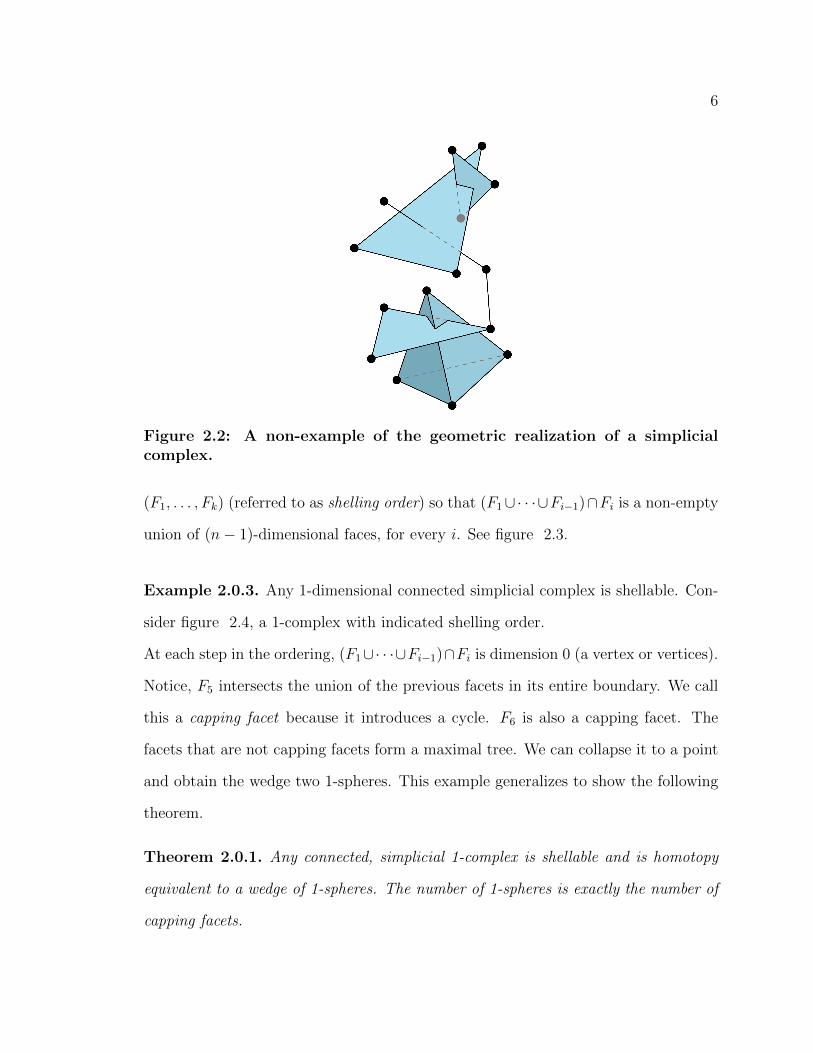
Example 2.0.3. Any 1-dimensional connected simplicial complex is shellable. Con-

sider figure 2.4, a 1-complex with indicated shelling order.

At each step in the ordering, (F1∪· · ·∪Fi−1)∩Fi is dimension 0 (a vertex or vertices).

Notice, F5 intersects the union of the previous facets in its entire boundary. We call

this a capping facet because it introduces a cycle. F6 is also a capping facet. The

facets that are not capping facets form a maximal tree. We can collapse it to a point

and obtain the wedge two 1-spheres. This example generalizes to show the following

theorem.

Theorem 2.0.1. Any connected, simplicial 1-complex is shellable and is homotopy

equivalent to a wedge of 1-spheres. The number of 1-spheres is exactly the number of

capping facets.

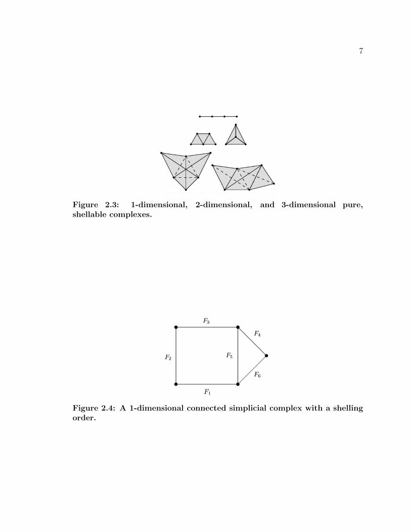
7

Figure 2.3: 1-dimensional, 2-dimensional, and 3-dimensional pure,shellable complexes.

Figure 2.4: A 1-dimensional connected simplicial complex with a shellingorder.

8

Figure 2.5: Caption

Example 2.0.4. The torus is not shellable. Consider the following simplicial com-

plex, with edge identifications made. We will attempt to put a shelling order on this

complex as follows in figure 2.5.

Notice F5 intersects the union of the previous facets in an edge and a vertex. A vertex

is not a 1-dimensional space, thus, this is not a shelling order for a torus. In fact, no

shelling order exists, and the following theorem holds.

Theorem 2.0.2. If an n-dimensional pure simplicial complex is shellable, then it is

homotopy equivalent to a wedge of n-spheres. The number of n-spheres is exactly the

number of capping facets (there could be none, in which case the complex is homotopic

to a point).

A detailed proof can be found in Koslov [6]. Nevertheless, here is a sketch of the

proof.

Proof. Let (F1, F2, . . . , Fk) be a shelling order for ∆. The proof uses two observations:

9

1. The union of (n − 1)-dimensional faces of an n-simplex which is not all of the

boundary is contractible;

2. The union ∆1 ∪ ∆2 of two contractible complexes is contractible in case the

intersection ∆1 ∩∆2 is contractible.

Let Fi1 , . . . , Fil be exactly the facets so that

(Fi1 ∪ · · · ∪ Fij−1) ∩ Fij

is the entire boundary of Fij . Let ∆0 be the union of these special facets. Using the

two observations above one can show that ∆ − ∆0 is contractible. Contracting the

subcomplex ∆0 in ∆ results in a space that is homotopy equivalent to ∆ and is a

wedge of l n-spheres.

Q.E.D.

10

Chapter 3

SURVEY OF ENGSTROM

This chapter presents some of the main results of Engstrom [5]. It does not contain

original material but in places provides more detailed arguments.

Definition 3.0.1. A directed graph Γ = (V,E, i, t) consists of sets V , E, and maps

i : E → V , and t : E → V . We refer to V as vertices, E as edges, i(e) as the initial

vertex of e and t(e) as the terminal vertex of e. We think of the edge e as directed

from i(e) to t(e).

If e is an edge and i(e) = x, t(e) = y we often write sometimes write e = (x→ y).

Graphs can be drawn in the plane: single out a point in the plane for each vertex and

draw a directed arc for every edge, connecting i(e) to t(e), putting an arrow on the

arc to indicate the direction. Some arcs might cross at points that are not vertices.

If such crossings can be avoided we call the graph planar.

Definition 3.0.2. Given a directed graph Γ.

1. A directed tree T in Γ is a directed subgraph that has a vertex r that can

connected to every other vertex v of T by a unique directed path from r to v.

The vertex r is called the root of T .

2. A directed forest F in Γ is the disjoint union of directed subtrees of Γ.

11

Figure 3.1: An example of a directed forest.

Definition 3.0.3. Given a directed graph Γ = (V,E, i, t).

1. The directed forest complex of Γ, DF(Γ), is a simplicial complex defined in the

following way: The vertex set V corresponds to the set of edges in the graph,

and a finite subset {e0, ..., ek} ⊆ E is a simplex if F =⋃i=0,...,k ei is a directed

forest in Γ.

2. Let R ⊆ V . Then the rooted directed forest complex, DFR(Γ), is a subcomplex

of DF(Γ) defined in the following way: The vertex set is V and {e0, ..., el} is a

facet if F =⋃i=0,...,l ei is a maximal directed forest in Γ with root set equal to

R.

Note that DF(Γ) is indeed a simplicial complex because every subgraph of a

directed forest is a directed forest. We specified only the facets of DFR(Γ). They

generate the simplicial complex DFR(Γ).

Example 3.0.1. Let Γ be the directed graph in figure 3.3.

The facets of DF(Γ) are shown in figure 3.3.

The facets of DF{1,4}(Γ) are shown in figure 3.4.

Definition 3.0.4. If K is a subcollection of a simplicial complex ∆ that contains

all faces of its elements, then K is another simplicial complex called a simplicial

subcomplex. An edge (x → y) of a directed graph Γ is nice in a subcomplex ∆ of

DF(Γ) if the following properties hold

12

Figure 3.2: A directed graph.

Figure 3.3: The facets of DF(Γ).

Figure 3.4: The facets of DF{1,4}(Γ)

13

1. if indeg(y) > 1, and

2. if F ∈ ∆ is a forest without an edge directed to y, then F ∪ (x→ y) ∈ ∆.

Algorithm for finding nice edges. There is a general procedure for finding nice

edges. We explain it using an example. Let Γ be the directed graph in example 3.0.1.

Let’s find some nice edges in DF{1,4}(Γ). We partition the vertices of the graph into

left and right. A vertex is on the left if

1. the tree which contains v has the same root, r, in all facets of DF{1,4}, and

2. the path from r to v is the same in all facets of DF{1,4}.

All other vertices are on the right. Then we consider the union of all the edges

of the facets. Notice that this is a subgraph of Γ. As we will see, the edges which

crossover the dotted line are nice.

Example 3.0.2. The construction for DF{1,4}(Γ) in Example 3.0.1 is given in figure

3.5.

Lemma 3.0.1. All edges crossing the dotted line in the nice construction are nice if

the maximal faces have the same roots.

Proof. First, we will show that the edges can only cross the dotted line from left to

right. For the sake of contradiction, assume that the edge (z → w) crosses from right

to left. Since w is on the left, the tree which contains w has the same root r in all

facets and the path from r to w is the same in all facets. Because w is on the left,

the vertex directed to it is always the same since all paths from r to w are the same.

Thus, the vertex directed to w is z since we know the edge (z → w) is in a maximal

facet. Because all paths from r to w are the same, all paths from r to z are the same.

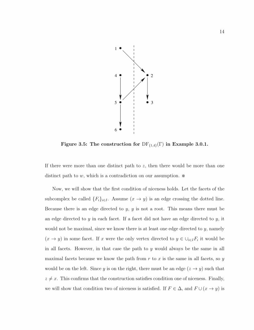
14

Figure 3.5: The construction for DF{1,4}(Γ) in Example 3.0.1.

If there were more than one distinct path to z, then there would be more than one

distinct path to w, which is a contradiction on our assumption. ※

Now, we will show that the first condition of niceness holds. Let the facets of the

subcomplex be called {Fi}i∈I . Assume (x → y) is an edge crossing the dotted line.

Because there is an edge directed to y, y is not a root. This means there must be

an edge directed to y in each facet. If a facet did not have an edge directed to y, it

would not be maximal, since we know there is at least one edge directed to y, namely

(x → y) in some facet. If x were the only vertex directed to y ∈ ∪i∈IFi it would be

in all facets. However, in that case the path to y would always be the same in all

maximal facets because we know the path from r to x is the same in all facets, so y

would be on the left. Since y is on the right, there must be an edge (z → y) such that

z 6= x. This confirms that the construction satisfies condition one of niceness. Finally,

we will show that condition two of niceness is satisfied. If F ∈ ∆, and F ∪ (x→ y) is

15

acylic, then the condition is fulfilled. A directed cycle which contains (x→ y) as an

edge would cross the dotted line at least twice, but all the edges crossing the dotted

line go from left to right. Hence, (x→ y) cannot induce a cycle, and thus, condition

two is fulfilled. We can now conclude that all edges crossing the dotted line in the

nice construction are nice if the maximal faces have the same roots.

Q.E.D.

Lemma 3.0.2. Let Γ = (V,E, i, t). If R ⊆ V is nonempty, and DFR(Γ) has more

than one facet, then there is an edge (x→ y) ∈ E(Γ) which is nice in DFR(Γ).

Proof. Suppose all vertices are on the left. Let F1 and F2 be facets of DFR(Γ). We

want to show that F1 = F2. Let e be an edge in F1. We will show that e is also in

F2. Let v be terminal vertex of e. Then v is contained in a tree T of F1 with root

r. Let p be the path T that connects r to v. Note that p contains e. The vertex v is

also contained in a tree T ′ of F2. Since v is on the left, the root of T ′ is also r and

the path connecting r to v in T2 is p. In particular p is contained in T2, and so, since

e is contained in p, e is in T2. This shows that F1 is contained in F2. Showing that

F2 is in F2 can be done by the same arguments. Q.E.D.

Here is a slightly different way to look at shellability, which also works in the

non-pure setting.

Definition 3.0.5. A simplicial complex ∆ is non-pure shellable if its maximal faces

can be ordered F1, F2, . . . Fn such that for all 1 ≤ i < k ≤ n there are 1 ≤ j < k and

e ∈ Fk such that Fi ∩ Fk ⊆ Fj ∩ Fk = Fk \ {e}.

Note that if ∆ is pure, then this definition agrees with the first definition [1]. We

give a proof.

16

Theorem 3.0.3. Pure shellable as defined in Chapter 2 and non-pure shellable as

defined here are equivalent if the simplicial complex in question is pure.

Proof. Assume ∆ is a pure n-complex, and it is non-pure shellable as in Definition

3.0.5. We want to show the complex is pure shellable as in Definition 2.0.1. Let

F1, . . . , Fm be a non-pure shelling order of ∆. We want to show that (F1 ∪ · · · ∪

Fk−1) ∩ Fk is the union of (n− 1)-dimensional faces of Fk.

By the distributivity of set operations,

(F1 ∪ · · · ∪ Fk−1) ∩ Fk = (F1 ∩ Fk) ∪ · · · ∪ (Fk−1 ∩ Fk).

Then there exists 1 ≤ j < k such that F1∩Fk ⊆ Fj ∩Fk = Fk−{e}. Therefore either

F1 ∩ Fk is (n− 1)-dimensional or it is contained in an (n− 1)-dimensional set in this

union, in which case we remove F1 ∩ Fk from the union (F1 ∩ Fk)∪ · · · ∪ (Fk−1 ∩ Fk).

We proceed in this fashion for F2∩Fk up to Fk−1∩Fk to see that (F1∩· · ·∩Fk−1)∩Fk

is indeed a union of (n − 1)-dimension faces. This show that the non-pure shellable

definition implies the pure shellable definition.

Now, we will show the other direction. Assume ∆ is pure, and we have a pure

shelling order F1, F2, . . . , Fm. Then,

(F1 ∪ F2 ∪ · · · ∪ Fk−1) ∩ Fk = (F1 ∩ Fk) ∪ · · · ∪ (Fk−1Fk)

= (Fi1 ∩ Fk) ∪ · · · ∪ (Fih ∩ Fk)

where {i1, . . . ih} ⊂ {1, . . . k−1} and Fi`∩Fk is (n−1)-dimensional. Then, (Fi∩Fk) ⊂

(Fi` ∩ Fk) = Fk − {e} is (n − 1)-dimensional. Take j = i`, and this shows that the

pure shellability definition implies the non-pure shellability definition.

17

Q.E.D.

Lemma 3.0.4. Let Fi and Fk be distinct facets in DFR(Γ) and (x→ y) ∈ Fi \ Fk a

nice edge in DFR(Γ). Then there is a facet Fj ∈ DFR(Γ) and an edge e ∈ Fk such

that Fi ∩ Fk ⊆ Fj ∩ Fk = Fk \ {e}.

Proof. Assume Fi and Fk are distinct facets in DFR(Γ) and (x → y) ∈ Fi \ Fk a

nice edge in DFR(Γ). There is an edge (z → y) ∈ Fk since it is a facet and y

in not a root. Replace (z → y) with (x → y) to construct Fj ∈ DFR(Γ). Now,

Fj ∩ Fk = Fk \ {(z → y)}. Since the nice edge (x → y) ∈ Fi and (z → y) /∈ Fi, we

can conclude that

Fi ∩ Fk = Fi ∩ (Fk \ {(z → y)}) (since we know (z → y) /∈ Fi)

⊆ Fk \ (z → y)) (by definition of intersection)

= Fj ∩ Fk (by definition of Fj)

Thus, there is a facet Fj ∈ DFR(Γ) and an edge e ∈ Fk such that

Fi ∩ Fk ⊆ Fj ∩ Fk = Fk \ {e},

namely (z → y).

Q.E.D.

Theorem 3.0.5. (Engstrom [5]) The complex DFR(Γ) is (non-pure) shellable for any

∅ 6= R ⊆ V (Γ).

Proof. We start by induction over the facets. Case 1. DFR(Γ) has only one facet. It

is then a simplex and shellable.

18

Case 2. DFR(Γ) has more than one facet. We know that DFR(Γ) has a nice edge

(x→ y) as show in lemma 3.0.2. Let’s define Γ′,Γ′′ ⊂ Γ as follows,

E(Γ′) = E(Γ) \ {(z → y)|z 6= x}, and

E(Γ′′) = E(Γ) \ {x→ y}.

A facet of DFR(Γ) has exactly one edge to y by defition of a directed tree, and thus a

facet DFR(Γ) is contained in either DFR(Γ′) or DFR(Γ′′). Because (x→ y) is nice, it

is in some, but not all facets of DFR(Γ). Both DFR(Γ′) and DFR(Γ′′) have a smaller

number of facets than DFR(Γ), so by induction, they are shellable. Taking stock, we

have a shelling order of DFR(Γ′), namely, F1, F2, . . . , Ft all of which contain (x→ y).

We also have a shelling order of DFR(Γ′′), that is, Ft+1, Ft+2, . . . , Ft+s which do not

contain the nice edge. We want to show that for all 1 ≤ i < k ≤ s + t there are

1 ≤ j < k and (z → w) ∈ Fk such that

Fi ∩ Fk ⊆ Fj ∩ Fk = Fk \ {z → w}.

This would show that DFR(Γ) is shellable where the shelling order is

F1, . . . , Ft, Ft+1, . . . , Ft+s.

Subcase 1. The inequality 1 ≤ i < k ≤ t or t + 1 ≤ i < k ≤ t + s holds. If this is

true, we’re done as we already showed this was shellable.

Subcase 2. The inequality 1 ≤ i ≤ t < k ≤ s + t holds. We know the nice edge is in

Fi, but not in Fk. Then we can construct Fj as described in Lemma 3.0.4. The edge

19

Figure 3.6: The facet F = T1 ∪ T2 ∪ · · · ∪ Tn ∈ DF(Γ) and ri, the root of Ti,for every i

(x→ y) is in Fj, so j ≤ t < k, and we have the shelling

F1, . . . , Ft, Ft+1, . . . , Ft+s.

Q.E.D.

Corollary 3.0.6. (Engstrom [5]) If Γ is a directed acyclic graph, then DF(Γ) is

shellable.

Proof. Assume that Γ is an acyclic graph, then Γ has roots. We want to show that

DF(Γ) = DFR(Γ).

Part 1. The inequality DF(Γ) ⊇ DFR(Γ) holds: Because every facet, F ∈ DFR(Γ),

with root set R is a forest, F ∈ DF(Γ).

Part 2. The inequality DF(Γ) ⊆ DFR(Γ) holds: Let F = T1 ∪ T2 ∪ · · · ∪ Tn ∈ DF(Γ)

be a facet and let ri be the root of Ti, for every i. We can visualize this in figure 3.6

We want to show that all ri ∈ R. For the sake of contradiction, assume that r1 /∈

R. If it is not in the rootset, there is an edge which terminates at r1. Let’s call this

vertex v1.

Subcase 1: There are no other vertices terminating at v1. As shown in figure 3.7.

20

Figure 3.7: Subcase 1.

Figure 3.8: Subcase 2.

In this case, we have a contradiction on maximality since F ∪ (v1 → r1) is a forest

and it has more edges than F itself.※

Subcase 2: The vertex vi ∈ Ti for some i 6= 1. As shown in figure 3.8, for example.

Similarly, this is contradiction on maximality.

Subcase 3: The vertex vi ∈ T1. As shown in figure 4.1, for example.

This is a contradiction on cyclicity, as this would form a directed cycle. Thus, if

Γ is a directed acyclic graph, then DF(Γ) is shellable.

Q.E.D.

21

Figure 3.9: Subcase 3.

22

Chapter 4

THE DIRECTED FOREST COMPLEX OF A CAYLEY

GRAPH

4.1 Cayley graphs

Definition 4.1.1. Given a group G and a generating set X. We define the Cayley

graph Γ = Γ(G,X) = (G,G×X, i, t) where i(g, x) = g and t(g, x) = gx.

Note that, using the notation of the previous chapter, we have (g, x) = (g → gx).

The group G acts on Γ via left multiplication: g′ · g = g′g, and g′ · (g, x) = (g′g, x).

This action is “continuous” in the following sense: i(g′ · (g, x)) = g′ · i(g, x) and

t(g′ · (g, x)) = g′ · t(g, x). It induces a continuous (or simplicial) action on the directed

forest complex DF(Γ) and we will say more about this later. It is common to label

the edge (g, x) with just x, if it is clear where it starts.

Example 4.1.1. Let G = D3 = 〈a, b|a2, b2, (ab)3〉. Then the Cayley graph Γ =

Γ(D3, {a, b}) can be see in figure 4.2

Example 4.1.2. Let G = Z3 × Z3 = 〈x, y|x3, y3, xyx−1y−1〉. Then the Cayley graph

Γ = Γ(Z3 × Z3, {x, y}) is seen in figure 4.3.

Note that this graph is not planar but can be drawn on a torus.

Definition 4.1.2. A Hamiltonian cycle in a Cayley graph is a simple closed edge

loop that goes through every vertex exactly once. So if G = {g1, ..., gn} and X is a

23

Figure 4.1: General edge in a Cayley graph

Figure 4.2: Γ = Γ(D3, {a, b})

Figure 4.3: Γ = Γ(Z3 × Z3, {x, y})

24

generating set then a Hamiltonian cycle is of the form (g1, x1)(g2, x2)...(gn, xn), where

xi ∈ X, gixi = gi+1, and gnxn = g1.

The following question is open:

Question. Do all Cayley graphs admit a Hamiltonian cycle? (Curran-Gallian [4])

The following however is known.

Theorem 4.1.1. (Pak-Radoicic [8]) For every finite group G there exists a generating

set X so that the associated Cayley graph does admit a Hamiltonian path.

What motivated some of this work is the fact that the homology of the directed

forest complex can see Hamiltonian cycles.

Theorem 4.1.2. Every Hamiltonian cycle in a Cayley graph Γ gives a nontrivial

element in H|G|−2(DF(Γ)).

Proof. Suppose |G| = n and e1 . . . en is a Hamiltonian cycle in Γ. Let σ = {e1, ..., en}.

Now σ is not a simplex in DF(Γ), but its boundary ∂σ is a subcomplex of DF(Γ).

Note that σ has dimension |G| − 1, so ∂σ has dimension |G| − 2. Since ∂∂σ = 0,

∂σ defines a non-trivial cycle in the top dimension, and hence a non-trivial homology

element. Q.E.D.

When we started work on this thesis, our hope was: Let Γ be a Cayley graph.

Then DF(Γ) is shellable and the dimension of the top dimensional homology equals

the number of Hamiltonian cycles in Γ. In retrospect this seems naive, but sometimes

it is true.

Example 4.1.3. Consider the Cayley graph of Γ(Z4) in figure 4.4.

25

Figure 4.4: Cayley graph Γ(Z4).

Figure 4.5: Top dimensional forests of DF(Z4).

26

Figure 4.6: The geometric realization of DF(Z4).

Notice, this graph has a Hamiltonian cycle. We can draw the top dimensional

forests which correspond to facets in the simplicial complex in figure 4.5.

Because each facet has three vertices, they are all realized geometrically by a (filled

in) triangle. We can see the geometric realization of this complex as the boundary of

a 3-simplex.

In this example, we see that DF(Γ) is shellable (we can choose any ordering of

the facets in the boundary of a simplex to get a shelling order), and we see that the

unique Hamilton cycle in the graph generates the unique homology element in DF(Γ).

More generally the dream theorem is true in the following setting.

Theorem 4.1.3. Let G = Zn = 〈x | xn = 1〉, and let Γ be the associated Cayley

complex. Then DF(Γ) is the boundary of an (n − 1)-simplex, and thus is shellable.

The dimension of Hn−2(DF(Γ)) is one and Γ contains exactly one Hamiltonian cycle.

In general the situation is more complicated. The next result is due to Koslov [7].

He studied (among other things) the homotopy type of the directed forest complex

for double directed circles.

27

Theorem 4.1.4. Let G = Dm = 〈x, y | x2 = y2 = (xy)m = 1〉 be the dihedral group

and Γ the associated Cayley graph. Then DF(Γ) is homotopic to:

S2k−1 ∨ S2k−1 ∨ S3k−2 ∨ S3k−2 if 2m = 3k,

S2k ∨ S3k−1 ∨ S3k−1 if 2m = 3k + 1,

S2k ∨ S3k ∨ S3k if 2m = 3k + 2.

Proof. Note that Γ is a double directed cycle as considered in Koslov [7] and the

result follows from his Proposition 5.2. Q.E.D.

Note that in case of D2, so 2m = 4 = 3 · 1 + 1, we get that DF(Γ) has the

homotopy type of S2 ∨ S2 ∨ S2. We will see this directly in the next chapter, where

we aslo show that in that case DF(Γ) is shellable. Using a computer we computed the

homology of DF(Γ) in the case of D3 and found that the Betti vector for H∗(DF(Γ),R)

is 〈1, 0, 0, 2, 2〉. We did this before we knew Koslov’s result that gives the homotopy

type S3 ∨ S3 ∨ S4 ∨ S4, which matches with our computation. Note that this implies

that DF(Γ) for D3 is not shellable: because DF(Γ) is pure of dimension 4 (see next

section) shellability would imply that there is no 3-dimensional homology.

4.2 The question of purity

Theorem 4.2.1. Let Γ be the Cayley graph of a finite group. Then

1. A maximal directed forest in Γ contains all the vertices of Γ;

2. Every directed tree T is contained in a maximal directed tree that contains all

the vertices of Γ.

28

Proof. 1. Let F be a maximal directed forest in a Cayley graph Γ. Suppose for the

sake of contradiction that there exists a vertex v ∈ Γ that is not contained in F . Let

e be an edge directed to v. We know e exists because Γ is a Cayley graph, and so

at every vertex, there is at least one outgoing and one incoming edge. The edge e

is either disjoint from F or connects to a component in F . In either case e ∪ F is a

larger directed forest in Γ that contains F , contradicting maximality.

2. Suppose that T a directed tree in Γ that is not contained in a bigger directed

tree. We will show that T contains all vertices of Γ. Let r be the root of T . Suppose

that v is a vertex not contained in T . Note that there is a shortest directed path γ

in Γ from r to v. This is because Γ is the Cayley graph of a finite group: if x is a

generator, then xn = 1 for some n > 1 and so x−1 = xn−1. So all elements g ∈ G can

be expressed as positive words in the generators. If γ does not intersect Γ except at

r, then T ∪ γ is a bigger directed tree containing T . If γ does intersect T , let w be

the last vertex on γ ∩ T , and let γ′ be the tail end of γ that connects w to v. Then

T ∪ γ′ is a bigger directed tree.

Q.E.D.

Corollary 4.2.2. If Γ is a Cayley graph then the dimension of DF(Γ) is |G| − 2.

Furthermore, DF(Γ) is pure if and only if all the facets come from maximal directed

trees.

Proof. Let {e0, ..., en} be a facet of DF(Γ) and let F =⋃i ei be the associated directed

forest. By Theorem 4.2.1, F contains all the vertices of Γ. Let c be the number of

components of F . We have

c = χ(F ) = |G| − (n+ 1),

29

Figure 4.7: The Cayley graph of D3 = 〈a, b | a2, b2, (ab)3〉.

so n = |G| − c − 1. Thus n ≤ |G| − 2. By Theorem 4.2.1 there exists a facet such

that F is a tree, in which case c = 1 and n = |G| − 2. This also shows that all facets

have the same dimension |G| − 2 if and only if all facets come from trees.

Q.E.D.

Not all DF(Γ) are pure. Consider figure 4.7 showing the Cayley graph of

D3 = 〈a, b | a2, b2, (ab)3〉.

Note that there is a maximal directed tree containing 5 edges, so DF(Γ) contains a

4-dimensional facet. The red edges shown in the picture show a maximal directed

forest (no edge can be added to make it a bigger directed forest) containing only 4

edges. So DF(Γ) contains a 3-dimensional facet.

4.3 Actions and stabilizers

The action of G on a Cayley graph Γ (by left multiplication) induces an action

of DF(Γ). In this and the next sections we address the question of stabilizers and

30

connectedness properties of DF(Γ).

We recall some relevant definitions. A action of a group on a set X is a homo-

morphism φ : G → Bij(X), where Bij(X) is the group of bijections. We write gx

instead of φ(g)(x) in case the action is understood.

If ∆ is a simplicial complex then a homeomorphism f : ∆ → ∆ is a bijection

f : V → V on the set of vertices so that if {v0, ..., vk} is a simplex then so is

{f(v0), ..., f(vk)}. An action ofG on ∆ is a group homomorphism φ : G→ Homeo(∆),

where Homeo(∆) is the group of homeomorphisms of ∆. If σ is a simplex we write

gσ instead of φ(g)(σ). The orbit of a simplex σ is the set

Gσ = {gσ | g ∈ G}.

The stabilizer of a simplex σ is the subgroup

stab(σ) = {g ∈ G | gσ = σ}.

We say a group acts freely on a set if all stabilizers stab(x) are trivial.

As always, let G be a finite group, Γ be a Cayley graph for G associated with a

generating set, and DF(Γ) be the directed forest complex.

Theorem 4.3.1. G acts freely on the vertices of DF(Γ).

Proof. The vertices of DF(Γ) are the edges in Γ. The group G acts freely on Γ, in

particular on its edge set: g′(g, x) = (g′g, x) = (g, x) implies that g′g = g, and it

follows that g′ = 1 Q.E.D.

31

The next result is general and applies outside the strict setting of directed forest

complexes. Let G be a finite group and ∆ be a simplicial complex on which G acts.

Theorem 4.3.2. Let k be the smallest number so that there exists a k-simplex, σ, so

that the stabilizer of σ is not trivial. Then k + 1 divides the order of G.

Proof. Let σ = {v0, ..., vk}. Let H be the stabilizer of σ and let h be a non-trivial

element of order m of H. Consider the orbit

〈h〉{v0} = {v0, hv0, h2v0, . . . , h

m−1v0} ⊆ σ = {v0, ...vk}.

This orbit has to be equal to σ by the assumption on k: if the orbit is properly

contained in σ then h is contained in the stabilizer of a proper face of σ, but we

assumed the stabilizers of such are trivial. It follows that m = k + 1, where m is the

order of h. So k + 1 divides the order of H and hence the order of G. Q.E.D.

Example 4.3.1. Let G = Zp, where p is a prime. Let Γ be a Cayley graph of G

coming from generating set with a single element. Then Γ is a single p− cycle. Then

DF(Γ) is the boundary of a p− 1 simplex (topologically a p− 2-sphere), and G acts

freely on DF(Γ).

Example 4.3.2. In case G = Zn, where n is not a prime we still have a Cayley graph

that is a single n-cycle, and DF(Γ) is still the boundary of an n− 1-simplex, but the

stabilizers are not trivial anymore. For example, if G = Z4 = 〈x〉, then the stabilizer

of {(1, x), (x2, x)} contains x2.

Example 4.3.3. Let G = Z5 × Z5, then dim(DF(Γ)) = 23. We know that G acts

freely on the 0-skeleton of DF(Γ). Now 1 + 1 = 2, 2 + 1 = 3, 3 + 1 = 4 do not divide

the order of G which is 25. Thus G acts freely on the 3-skeleton of DF(Γ). Note that

32

4 + 1 = 5 does divide the order of G, so G might stabilize a 4-simplex (but we can

not be sure without checking).

The following theorem is due to Serre.

Theorem 4.3.3. If a group G acts orientation-preserving on a tree T, then it fixes

a vertex.

Proof. We will sketch a proof in the case that G and T are finite. Let L be a longest

line in T , and let v be its midpoint. Then gv is the midpoint of the line gL. Choose

a connecting line L0 from v to gv, then half of L together with L0 and half of gL is

a line that is longer than L unless the length of L0 is 0. Thus, v = gv.

Q.E.D.

Theorem 4.3.4. Let F = {e0, ..., en} be a facet of DF(Γ) so that T =⋃i ei is a tree.

Then, stab(F ) = 1.

Proof. Let g ∈ stab(F ), then gF = F . In particular,⋃gei =

⋃ei. Then, gT = T .

By Serre’s theorem, g fixes a vertex of T . Hence, g = 1, and therefore stab(F ) = 1.

Q.E.D.

We summarize the findings from this section. If Γ is the Cayley graph of a finite

group, then G acts freely on the vertices and facets of DF(Γ) that come from directed

trees. We also have the following divisibility condition: if p is the smallest prime

factor of |G|, then G acts freely on simplices of dimension up to p− 2. However, the

action on larger simplices may fail to be free.

4.4 Simple connectivity

Let G be a finite group and Γ = Γ(G,X) a Cayley graph. Let n = |X|.

33

Theorem 4.4.1. If for every four edges e1, e2, e3, e4 ∈ Γ there exists an edge e disjoint

from the union of the ei, then DF(Γ) is simply connected.

Proof. Suppose {e1, e2}, {e2, e3}, {e3, e4}, . . . , {em, e1} is a simple edge loop in DF(Γ).

Suppose that m ≥ 4. Choose e disjoint from the union e1∪e2∪e3∪e4. Then we have

2-simplices {ei, ei+1, e}, i = 1, 2, 3 in DF(Γ) and we can cone off the first 3 edges in

the loop using the triangles. This gives a shorter loop {e1, e}{e, e4}{e4, e5}...{em, e1}.

If m = 3 (the smallest possible number) then we cone the entire loop off.

Q.E.D.

Corollary 4.4.2. If |G| > 16− 4n

, then DF(Γ) is simply connected.

Proof. Consider four edges e1, ..., e4 in Γ. Note that there are 2n − 1 edges distinct

from e1 at each vertex of e1. Thus there are 2(2n − 1) + 1 edges connected to e1

(including e1). It follows that there can not be more than 4(4n− 1) = 16n− 4 edges

connected to the union e1∪ e2∪ e3∪ e1∪ e4. Note that we have n|G| edges in Γ. Thus

if n|G| > 16n− 4, then there is an edge e in Γ disjoint from the union.

Q.E.D.

Example 4.4.1. If G = Z5×Z5 = 〈a, b | a5 = 1, b5 = 1, ab = ba〉. Here |G| = 25 > 16,

so DF(Γ) is simply connected.

4.5 A fundamental domain

Suppose a group G acts on a simplicial complex ∆. A fundamental domain is a

subcomplex D which contains exactly one simplex from every orbit Gσ, where σ is a

maximal simplex in ∆.

Consider DFg(Γ). Recall that this is the subcomplex of DF(Γ) whose facets come

from trees in Γ with root g, where Γ is a Cayley graph.

34

Theorem 4.5.1. DF 1(Γ) is shellable and contractible.

Proof. Engstrom’s Theorem 3.0.5 on rooted directed forest complexes gives shellabil-

ity. We are left to show contractibility. Let {x1, ..., xn} be the generating set used

in building of Γ. We assume that all the xi are distinct. Let ei = (1, xi). Note

that {e1, ..., en} is a simplex in DF1(Γ). Then every maximal tree in Γ with root 1

contains at least one of the ei. LetKi be the subcomplex of DF1(Γ) where the maximal

simplices contain ei. Note that Ki is the star of the vertex ei in DF1(Γ) and so Ki is

contractible (see [6]). We have DF1(Γ) =⋃Ki. Note that Ki∩Kj is the subcomplex

of DF1(Γ) whose maximal simplices come from maximal trees that contain both ei and

ej. The set {ei, ej} is an edge in DF1(Γ), so the intersection Ki∩Kj is the star of that

edge. Hence the intersection is contractible. Similarly, the intersections Ki∩Kj ∩Kk

is the star of the simplex {ei, ej, ek}, and so is contractible. This argument extends to

all intersections, so all intersections are non-empty and contractible. Contractibility

of DF1(Γ) now follows from the nerve theorem (see Brown [?], Chapter VII, Theorem

4.4). Q.E.D.

Lemma 4.5.2. If DF(Γ) is pure we have DF(Γ) =⋃g∈G

DFg(Γ).

Proof. We recall Corolary 4.2.2: DF(Γ) is pure if and only if all facets come from

maximal directed trees in Γ. We can see that DF(Γ) ⊇⋃g∈G

DFg(Γ) because each

DFg(Γ) is a subcomplex of DF(Γ). Now we will show that DF(Γ) ⊆⋃g∈G

DFg(Γ).

Suppose that σ = {e0, . . . ek} is a facet in DF(Γ). Then T =k⋃j=0

ej is a maximal

directed tree in Γ. Hence it has a root, say g. It follows that σ ∈ DFg(Γ).

Q.E.D.

Lemma 4.5.3. h ·DFg(Γ) = DFhg(Γ)

35

Proof. Let σ = {e0, . . . , ek} be a facet in DFg(Γ). Then T =⋃ej is a maximal

directed tree with root g. Then hT =⋃hej is a maximal directed tree with root hg.

So, hσ = {he0, . . . , hek} ∈ DFhg(Γ).

Q.E.D.

The last two results give the following:

Corollary 4.5.4. DF1(Γ) is a fundamental domain for the action of G on DF(Γ) in

case DF(Γ) is pure.

Question. If DF(Γ) is n dimensional, then is it true that DFg(Γ) is n dimensional,

DFg(Γ)∩DFh(Γ) is n−1 dimensional, DFg(Γ)∩DFh(Γ)∩DFf (Γ) is n−2 dimensional,

and so on...

Example 4.5.1. Let G = D3 = 〈x, y | x2, y2, (xy)3〉 and let Γ be the associated

Cayley graph. Using a computer we found that H∗(DF(Γ),R) = 〈1, 0, 0, 2, 2〉. The

fact that the 3rd homology is not trivial might be a first hint that DF(Γ) is not pure.

It might be non-pure shellable as Koslov’s Theorem 4.1.4 seems to suggest.

One can attempt to obtain all homotopical information about DF(Γ) by trying

to find a shelling order. That approach might be too optimistic, even if we asume

DF(Γ) is pure. But in that case we can work with the cover DF(Γ) =⋃

DFg(Γ). If

intersections of the pieces DFg(Γ) are shellable, then we know the homotopy type of

the pieces and their intersections and thus can compute the homology of DF(Γ) using

the Mayer-Vietoris spectral sequence.

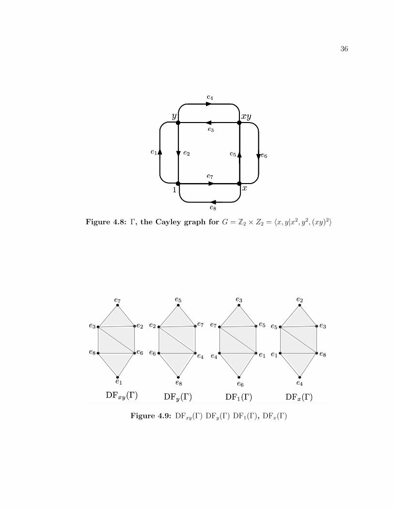
Example 4.5.2. Let Γ be the Cayley graph for G = Z2 × Z2 = 〈x, y|x2, y2, (xy)2〉,

seen in figure 4.8.

36

Figure 4.8: Γ, the Cayley graph for G = Z2 × Z2 = 〈x, y|x2, y2, (xy)2〉

Figure 4.9: DFxy(Γ) DFy(Γ) DF1(Γ), DFx(Γ)

37

Figure 4.10: Some identifications made on the setDFxy(Γ) DFy(Γ) DF1(Γ),DFx(Γ).

Figure 4.11: The capping forests.

38

From this, we can draw DFxy(Γ) DFy(Γ) DF1(Γ), DFx(Γ) respectively as seen in

figure 4.9.

Consider the following intersections,

DF1(Γ) ∩DFx(Γ) ={{e3, e5}, {e1, e5}, {e1, e4}

}DF1(Γ) ∩DFy(Γ) =

{{e5, e7}, {e4, e6}, {e4, e7}

}DF1(Γ) ∩DFxy(Γ) =

{{e1, e6}, {e3, e7}

}DF1(Γ) ∩DFx(Γ) ∩DFy(Γ) = {{e4}, {e5}}

Knowing the intersections (all are indeed shellable) we could compute the homol-

ogy using Mayer-Vietoris. But note that the complex DF(Γ) is shellable, and hence

homotopically a wedge of 2-spheres. A shelling order is indicated in the picture.

The 3 red 2-simplices shown are the “capping simplices”, the ones that produce the

2-spheres in the wedge. Note furthermore that Γ, being a double directed cycle,

contains exactly two Hamiltonian cycles, but the dimension of H2(DF(Γ),R) is 3.

Intersections of the various DFg(Γ) are difficult to understand. The above example

also shows that in general DF1(Γ) ∩DFg(Γ) 6= DF{1,g}(Γ).

Computation 1. The Betti vector of the directed forest complex of the Cayley graph

Z2 × Z2 = D2 = 〈x, y|x2, y2, (xy)2〉 is 〈1, 0, 3〉. In fact, we know that this is complex

is shellable.

Computation 2. The Betti vector of the directed forest complex of the Cayley graph

39

Z3×Z3 = 〈x, y|x3, y3, (xy)3〉 is 〈1, 0, 0, 0, 0, 0, 0, 28〉. We believe DF(Γ) is pure in this

case. We do not know if this complex is shellable.

Computation 3. The Betti vector of the directed forest complex of the Cayley graph

D3 = 〈x, y|x2, y2, (xy)3〉 is 〈1, 0, 0, 2, 2〉. We know that DF(Γ) is not pure. Is this

detected by the homology? Is DF(Γ) non-pure shellable?

Theorem 4.5.5. If Γ is the Cayley graph of a group G such that G 6= Z2, then

DFg1(Γ) ∩DFg2(Γ) 6= ∅ for every g1, g2 ∈ G.

Proof. It suffices to show that DF1(Γ)∩DFg(Γ) 6= ∅ for every g ∈ G. If G is cyclic with

minimal generating set then the statement is true as Γ is a cycle of length 3 or greater.

Now suppose Γ arises from a generating set containing at least two generators. There

exists an edge e∗ for which the the identity is the initial vertex and the element g is

not the terminal vertex. By definition, e∗ ∈ DF1(Γ). We can connect the vertex g

to the vertex e∗ by a directed edge path e1, . . . , ek that starts at g and ends at the

identity element. Then {e1, . . . , ek, e∗} ∈ DFg(Γ). Thus, e∗ ∈ DF1(Γ) ∩DFg(Γ).

Q.E.D.

For the definition of Hamiltonian cycle see Definition 4.1.2. Here are some exam-

ples of Cayley graphs with directed Hamiltonian cycle:

Γ for Dn = 〈x, y|x2 = 1, y2 = 1, (xy)n = 1〉.

Γ for

Zn × Zm = 〈x, y|xn = 1, ym = 1, xy = yx〉

.

Lemma 4.5.6. Suppose Γ is a Cayley graph that contains a directed Hamiltonian

cycle. Then

40

1. for every x ∈ G,⋂

g∈G,g 6=x

DFg(Γ) 6= ∅, and

2.⋂g∈G

DFg(Γ) = ∅.

Proof. (1) Set Z be a directed Hamiltonian cycle. Let e be the edge in Z that

terminates at the vertex x, then e ∈⋂g 6=x

DFg(Γ). (2) Note that if e is an edge in Γ

that terminates in g, then {e} /∈ DFg(Γ).

Q.E.D.

Definition 4.5.1. Suppose X is a simplicial complex and X =⋃j∈J

Xj is a cover of

X by subcomplexes. The nerve, N, is a simplicial complex is defined as follows,

1. The set of vertices is J , and

2. The set j0, . . . , jk is a simplex if Xj0 ∩ · · · ∩Xjk 6= ∅.

The nerve comes with a coefficient system. If σ = {j0, ..., jk} is a simplex of

N , we denote by Xσ = Xj0 ∩ ... ∩ Xjk . Note that if τ ⊆ σ then we have a map

Hq(Xσ)→ Hq(Xτ ) induced by inclusion. We can define a chain complex

Hq : ...→⊕σ∈X

Hq(Xσ)→⊕τ∈X

Hq(Xτ )→ ...

whose pth homology we denote by Hp(N,Hq). The spectral sequence

E2pq = Hp(N,Hq)⇒ Hp+q(X)

is called the Mayer-Vietoris spectral sequence. Details on this can be found in Brown

[3], Chapter VII. Thus, in order to compute Hn(X) one needs to get hold of the nerve

and understand the intersections of the various Xj.

41

We complete this thesis by computing the nerve of the cover DF(Γ) =⋃g∈G DFg(Γ)

in case DF(Γ) is pure.

Theorem 4.5.7. Let Γ be a Cayley graph with a directed Hamiltonian cycle. Assume

that DF(Γ) is pure. The nerve N of this covering, DF(Γ) =⋃

DFg(Γ), is ∂∆(G),

where ∆(G) is the simplex with vertex set G. Thus N is topologically a (|G| − 2)-

sphere.

Proof. Note that the nerve N can be described as follows, vertices are elements of G

and the simplicies {g0, . . . , gk} ∈ N if DFg0(Γ) ∩ · · · ∩DFgk(Γ) 6= ∅. Then by Lemma

4.5.6, N = ∂∆(G), where ∆(G) is the full simplex on vertex set G.

Q.E.D.

42

Bibliography

[1] Anders Bjorner and Michelle Wachs. Shellable nonpure complexes and posets. i.

Transactions of the American mathematical society, 348(4):1299–1327, 1996.

[2] Bela Bollobas. Modern graph theory, volume 184. Springer Science & Business

Media, 2013.

[3] Kenneth S Brown. Cohomology of groups, volume 87. Springer Science & Business

Media, 2012.

[4] Stephen J Curran and Joseph A Gallian. Hamiltonian cycles and paths in cayley

graphs and digraphs—a survey. Discrete Mathematics, 156(1-3):1–18, 1996.

[5] Alexander Engstrom. Complexes of directed trees and independence complexes.

Discrete Mathematics, 309(10):3299–3309, 2009.

[6] Dimitry Kozlov. Combinatorial algebraic topology, volume 21. Springer Science

& Business Media, 2007.

[7] Dmitry N Kozlov. Complexes of directed trees. Journal of Combinatorial Theory,

Series A, 88(1):112–122, 1999.

[8] Igor Pak and Rados Radoicic. Hamiltonian paths in cayley graphs. Discrete

Mathematics, 309(17):5501–5508, 2009.