
The Development of a Semi-empirical Barrel Engraving ...
97
i The Development of a Semi-empirical Barrel Engraving Resistance Method for Internal Ballistic Simulation Codes Nawaf S Alanazi orcid.org/0000-0002-4369-8037 Dissertation accepted in partial fulfilment of the requirements for the degree Master of Science in Mechanical Engineering at the North-West University Supervisor: Prof. Willem den Heijer Co-Supervisor: Mr Victor Schabort Graduation: June 2021 Student number: 27359875
Transcript of The Development of a Semi-empirical Barrel Engraving ...
i
The Development of a Semi-empirical Barrel Engraving Resistance Method for
Internal Ballistic Simulation Codes
Nawaf S Alanazi
orcid.org/0000-0002-4369-8037
Dissertation accepted in partial fulfilment of the requirements for the degree Master of Science in Mechanical Engineering at
the North-West University
Supervisor: Prof. Willem den Heijer
Co-Supervisor: Mr Victor Schabort
Graduation: June 2021
Student number: 27359875

ii
ACKNOWLEDGEMENT
First and foremost, I wish to express my sincerest gratitude to Rheinmetall Denel Munitions that
gave me the opportunity to conduct this research. I wish to convey my appreciation to the
research supervisor, Professor Willem den Heijer, the technical research supervisor, Mr Victor
Schabort, and Mr Hans Heunis for their valuable assistance and guidance.
I dedicate this dissertation to my parents that inspired and supported me; to my wife that sacrificed
her studies to relocate to South Africa with me whilst patiently giving me all the support and
encouragement I dearly needed; and lastly to my brothers that looked after my children while we
were abroad.
I wish to thank the Saudi Arabian Government, particularly the Military Industries Corporation,
who provided funding and gave me the opportunity to develop myself to serve my country.
I also wish to pass my sincerest appreciation to the beautiful country and people of South Africa.

iii
ABSTRACT
This research focused on the implementation of a semi-empirical projectile barrel engraving
resistance model for internal ballistic simulation codes. An alternative method is provided to
determine the engraving resistance profile by the direct measurement of projectile movement and
subsequent creation of the resistance curve. The identified research problem, subsequent
literature survey, and the development of a semi-empirical projectile barrel engraving resistance
model in internal ballistic simulation codes have not been previously investigated based on the
literature survey conducted.
The advantage of the developed approach is its relative simplicity and the elimination of the need
for detailed material and structural analyses, as well as measurements of the projectile driving
band material interaction with the gun barrel.
The developed approach greatly improves the confidence over the traditional method in defining
the shape of resistance curves for the simulation model of gun systems. This approach is based
on intermediate experimental data, whereas the traditional method estimates the resistance curve
definition only based on the final experimental velocity and maximum pressure.
KEYWORDS: Semi-empirical, barrel engraving, internal ballistic simulation, strain gauge,
resistive pressure, STANAG 4367.

iv
ABBREVIATIONS AND VARIABLES
𝐹𝑖. 𝑖 𝑡ℎ propellant force per unit mass
𝑇0𝑖 𝑖𝑡ℎ propellant adiabatic flame temperature
𝐹𝑖′ 𝑖𝑡ℎ propellant adjusted force per unit mass
𝜌𝑖 𝑖𝑡ℎ propellant density
𝛾𝑖 𝑖𝑡ℎ propellant specific heat ratio
𝑃′𝑅 Adjusted resistive pressure because of engraving and friction
𝑃𝑎 Ambient air pressure
Aw Area of the chamber wall and gun tube wall area
BD Band diameter
BL Band length
𝑃𝑅 Bore resistive pressure due to engraving and friction
𝐴𝑏𝑟 Breech face area
Z Burning rate of the mass fraction of the propellant grain
𝑉𝑐 − 𝑉0 Chamber volume enlargement due to projectile displacement
Tc Chamber wall temperature
COR Commencement of rifling
FCurve Curvature force
D Diameter of the propellant grain
d Distance
𝑥 Displacement of the projectile
𝑓𝑅 Down-tube resistance factor
𝑉0 Empty gun chamber volume
𝐸𝑑 Energy loss due to air resistance
𝐸ℎ Energy loss due to barrel walls and heat transfer to the chamber
𝐸𝑏𝑟 Energy loss due to engraving and friction of driving band
𝐸𝑟 Energy loss due to recoil
EB Exterior ballistics

v
FExt Extrusion force
𝑓𝛽 Factor of burn rate
𝑓𝛽𝑇 Factor of burning rate temperature
𝑓𝑟 Factor of down-tube resistance
𝑓𝐹𝑇 Factor of force temperature
𝜃 Forcing cone included angle
Ffriction Friction force
DL Groove diameter
G/L Groove to land width ratio
�� Gun chamber space-mean pressure
𝑥𝑟𝑝 Gun Displacement due to recoil
𝑇0𝐼 Igniter adiabatic flame temperature
𝑏𝐼 Igniter covolume
𝐶𝐼 Igniter initial mass
𝐹𝐼 Igniter propellant force per unit mass
𝛾𝐼 Igniter specific heat ratio
FInc Incision force
𝑉0 Initial chamber volume
IDE Integrated development environment
IB Interior ballistics
NB Intermediate ballistics
IBS Internal ballistics simulation
DG Land diameter
LPM Lumped parameter model
𝜀 Mass ratio of ballistic
FF Metrical code
MIC Military Industries Corporation
MC Mono Cast

vi
MV Muzzle Velocity
NC Nitrocellulose
NG Nitroglycerine
NQ Nitroguanidine
PrN Normalised resistance pressure
NATO North Atlantic Treaty Organisation
𝑛 Number of propellants
𝑉𝑃𝑖 Parasitics associated with the 𝑖𝑡ℎ propellant volume
PDV Photonic Doppler velocimeter
KNO3 Potassium nitrate
𝑃0 Pressure of the breech
A Projectile base area including rotating band
𝑃𝑏 Projectile base pressure
𝑃𝑔 Projectile gas pressure
𝑚𝑝 Projectile mass
vp Projectile velocity
𝑉𝑐 Projectile volume available for propellant gas
𝑟 Propellant burning rate
β and α Propellant chemical composition parameters
C_gas Propellant gas mass
Vg Propellant grain initial volume
C Propellant initial total mass
CT Propellants and igniter total mass
Pr Resistance pressure
𝑃𝑅 Resistive pressure
RDM Rheinmetall Denel Munition
FRif Rifling force
TW Rifling twist

vii
RDX Royal Demolition Explosive
k Small residual constant
C_solid Solid propellant mass
STANAG Standard Agreement of North Atlantic Treaty Organisation
SG Strain gauge
S Sulfur
S Surface area of the propellant grain
TB Terminal ballistics
t Time
𝑡𝑟 Time of recoil
𝑉𝑐 Total chamber volume after projectile displacement
F Total resistance of force
TNT Trinitrotoluene
𝑣𝑟𝑝 Velocity of the gun recoil
V Volume of the propellant grain
𝐺𝐿𝑅 Width ratio of land and groove

viii
TABLE OF CONTENTS
1.1 Background ...................................................................................................... 1
1.2 Ignition System ................................................................................................. 2
1.3 Gun System ...................................................................................................... 3
1.4 Propelling Charge System ............................................................................... 3
1.5 Projectile Motion ............................................................................................... 4
1.6 Interior Ballistic Cycle and Simulation Models (IBS) ..................................... 5
1.7 Problem Statement ........................................................................................... 7
1.8 Aim .................................................................................................................... 8
1.9 Research Objectives: ....................................................................................... 8
1.10 Methodology ..................................................................................................... 8
1.11 Study Limitations ............................................................................................. 9
1.12 Contributions of the Study ............................................................................... 9
1.13 Chapter Division ............................................................................................... 9
1.14 Summary ......................................................................................................... 10
2.1 Introduction of Lumped-Parameter Thermodynamic Simulation ................ 11
2.1.1 Equation of Motion ............................................................................................ 12
2.1.2 Pressure Gradient Model .................................................................................. 12
2.1.3 Combustion Models .......................................................................................... 13
2.1.4 Equation of State .............................................................................................. 15
2.1.5 Energy Model ................................................................................................... 16
2.2 Engraving and Bore Resistance Cycle .......................................................... 18
2.2.1 History of Engraving and Bore Resistance Cycle .............................................. 18

ix
2.2.2 Simulation on the engraving process of the projectile rotating band .................. 25
2.2.3 Concept of Engraving and Bore Resistance Cycle ............................................ 29
2.2.4 Resistive Pressure ............................................................................................ 30
2.3 Conclusion ...................................................................................................... 31
3.1 Background .................................................................................................... 32
3.2 Weapon System and Setup ............................................................................ 32
3.3 Gun preparation .............................................................................................. 33
3.4 Strain Gauge Installation Methodology ......................................................... 34
3.4.1 Employment of Strain Gauges, ......................................................................... 34
3.4.2 Strain Gauge Sensor ........................................................................................ 35
3.5 Test Setup ....................................................................................................... 37
3.6 Firing Trail ....................................................................................................... 39
3.7 Practical Test Instrumentation Limitation ..................................................... 40
3.8 Chapter Summary ........................................................................................... 41
4.1 Introduction .................................................................................................... 42
4.2 Test Setup ....................................................................................................... 42
4.3 Tests Results .................................................................................................. 42
4.3.1 Shot Number 1 Results ..................................................................................... 43
4.3.2 Shot Number 2 Results ..................................................................................... 44
4.3.3 Shot Number 3 Results: .................................................................................... 45
4.3.4 Shot Number 4 Results ..................................................................................... 46
4.3.5 Shot Number 5 Results ..................................................................................... 47
4.4 Test summary ................................................................................................. 48

x
4.5 Chapter summary ........................................................................................... 49
5.1 Introduction .................................................................................................... 50
5.2 Data Analysis .................................................................................................. 50
5.3 Data Summary ................................................................................................ 52
5.4 Model Construction ........................................................................................ 53
5.5 Model Verification ........................................................................................... 57
5.6 Results of the Semi-empirical Resistive Pressure Curve of 35mm
Cannon ............................................................................................................ 57
5.7 Implementation of the Semi-Empirical Resistive Pressure Curve of
35mm Cannon into the Developed Model ..................................................... 59
5.8 Limitations of the experimental data ............................................................. 60
5.9 Chapter summary ........................................................................................... 60
6.1 Research Overview......................................................................................... 61
6.2 Conclusion ...................................................................................................... 61
6.3 Future Work .................................................................................................... 62

xi
LIST OF TABLES
Table 2-1 The resistive pressure inside a gun system ............................................................. 19
Table 2-2 Material properties that affect the stability of the projectile ....................................... 24
Table 2-3 Comparison of simulation results ............................................................................. 28
Table 3-1 Locations of the strain gauges on the barrel ............................................................ 37
Table 3-2 Propellant mass in each shot ................................................................................... 39
Table 4-1 Results of the measurements at different shots ....................................................... 48
Table 5-1 RDM IB model vs Developed Model ........................................................................ 57
Table 5-2 The semi-empirical resistive pressure at different time intervals .............................. 59
Table 5-3 The effect of the resistance pressure sub-model on IB results ................................. 60

xii
LIST OF FIGURES
Figure 1-1 Sub-systems of a typical ballistic system .................................................................. 2
Figure 1-2 Ignition sub-system in the ballistic system ................................................................ 2
Figure 1-3 Rifled-bore and smooth-bore gun sub-systems in a ballistic system ......................... 3
Figure 1-4 Difference between the smooth-bore and rifled barrels ............................................ 5
Figure 1-5 Effect of the bore on projectile motion after exiting the gun muzzle (Koffler,
2015).............................................................................................................. 5
Figure 1-6 Internal layout of the loaded gun system .................................................................. 6
Figure 1-7 Chamber pressure profile for the gun system ........................................................... 6
Figure 2-1 Illustrating Flowchart of LPM of interior ballistics .................................................... 11
Figure 2-2 Pressure gradient profile ........................................................................................ 13
Figure 2-3 Schematic of a typical PDV system (Sättler, 2013) ................................................. 21
Figure 2-4 Rack with optical components (left) and oscilloscope (right) (Sättler, 2013)............ 21
Figure 2-5 Working principle of the PDV (Sättler, 2013) .......................................................... 22
Figure 2-6 Pressure and velocity as a function of time ............................................................ 22
Figure 2-7 Acceleration and velocity as a function of displacement ("Planar Doppler
Velocimetry,") ............................................................................................... 23
Figure 2-8 Partially enlarged drawing of touch between band and barrel ................................. 23
Figure 2-9 Dynamic response of projectile centre of gravity in the system with different
band materials during the engraving process ............................................... 25
Figure 2-10 Schematic drawing of rotating band engraving process (Quanzhao, 2017) ......... 26
Figure 2-11 Evolution of Von Mises stress for rotating band (Quanzhao, 2017) ..................... 27
Figure 2-12 Engraving resistance (Quanzhao, 2017) ............................................................. 28
Figure 2-13 Inside of the gun system ....................................................................................... 29
xiii
Figure 2-14 Total resistive forces acting on projectile motion (Crowley, 1999, November) ...... 30
Figure 2-15 Variation of the resistance force due to friction with projectile motion (Crowley) ... 31
Figure 3-1 experimental weapon setup .................................................................................... 33
Figure 3-2 The preparations of the gun ................................................................................... 33
Figure 3-3 Definition of strain................................................................................................... 35
Figure 3-4 Construction and the principle of the work of a strain gauge ................................... 36
Figure 3-5 Full-bridge configuration of strain gauges ............................................................... 36
Figure 3-6 Locations of the strain gauges on the barrel ........................................................... 37
Figure 3-7 Bridge of strain gauges on the barrel of the 35mm ................................................. 38
Figure 3-8 Test methodology and setup .................................................................................. 38
Figure 4-1 Shot Number 1 results ............................................................................................ 43
Figure 4-2 Shot Number 2 results ............................................................................................ 44
Figure 4-3 Shot Number 3 results ............................................................................................ 45
Figure 4-4 Shot Number 4 results ............................................................................................ 46
Figure 4-5 Shot Number 5 results ............................................................................................ 47
Figure 4-6 Breech Pressure and SGs vs time for shot number 4 ............................................. 48
Figure 5-2 Determination of shot exit pressure ........................................................................ 51
Figure 5-3 Iterative procedure for measuring the actual resistance pressures ........................ 52
Figure 5-4 Flow chart plan for the IB model ............................................................................. 56
Figure 5-5 Showing the semi-empirical resistive pressure curve of 35mm cannon .................. 58
Figure 5-6 The semi-empirical resistive curve of the 35mm cannon ........................................ 59

1
CHAPTER 1 INTRODUCTION
1.1 Background
The attention to ballistics began with the use of traditional tools such as spears, arrows, bows,
and slingshots. In the early 9th century, the revolution of the ballistics field was developed by the
discovery of gunpowder, which is an essential part of the ballistic systems. Chinese scientists
accidentally encountered gunpowder from the reaction of charcoal, potassium nitrates, and
sulphur, which recrystallised from boiling water. The generation of these materials, described as
extremely explosive, led to the development of the ballistics field. After four centuries, gunpowder
has been used as a chemical propelling charge, in which it is ignited and to push and accelerate
a projectile through the barrel of a gun. The extensive progress in the field opens the gates for a
new field of ballistics (Gray, E., Marsh, H., & McLaren, M., 1982) (Gunpowder, 2019) (Kelly,
2004).
Ballistics can be defined as the scientific investigation of projectile motion and classified into four
disciplines, namely interior, intermediate, exterior, and terminal ballistics. The principles of these
disciplines are described as follows:
Interior ballistics (IB) deals with the interaction on the gun behaviour, propelling charge,
and projectile from the ignition of the propelling charge to the point in time when the
projectile exits the gun muzzle.
Intermediate ballistics deals with the period just after the projectile exits the barrel where the combustion gasses influence the orientation of the projectile.
Exterior ballistics (EB) covers the projectile behaviour from the time that the projectile exits
the gun muzzle until it reaches the target.
Terminal ballistics (TB) encompasses the comprehensive data of all the aspects when the
projectile impacts the target. (Carlucci & Jacobson, 2018) (Okunev, 1943)
A ballistics system comprises four sub-systems as shown in Figure 1-1, namely the projectile, the
propelling charge, the gun, and the igniter,.

2
Figure 1-1 Sub-systems of a typical ballistic system
In the following sections, more details will be provided regarding these sub-systems.
1.2 Ignition System
The ballistics process starts when the projectile is loaded from the back of the barrel. Ignition
commences when the firing pin crushes the primary cartridge, which produces a flame that is
transferred through the flash hole to the propellant grain (see Figure 1-2). The main function of
the primary cartridge is to ignite the propellant grain.
The two types of primary cartridges are boxer and Berdan cartridge primers. Both types have
same role but different mechanism that boxer has one hole to transfer the ignition to the main
cartridge while Berdan has two holes between the primary and main cartridges.
(Worsfold, Townshend, Poole, & Miro, 2019.)
Figure 1-2 Ignition sub-system in the ballistic system

3
1.3 Gun System
The gun system in medium calibre applications contains the following components as shown in
Figure 1-3, namely the breech, the barrel and the chamber. A gun barrel is made from a high-
strength metallic tube that allows the projectile to travel. The front end of the barrel is called the
muzzle in which the projectile comes out from. The interior of the barrel, known as the bore, can
be classified into two types , as shown in Figure 1-3 (Deng, Sun, Chiu, & Chen, 2014).. The first
type is smooth bore which has flat surface throughout the barrel. The second type is rifled bore
which has circumferential grooves to spin the projectile throughout the barrel.
The barrel has a smaller diameter than the chamber to accommodate the propelling charge. Thus,
the diameter decreases from the chamber (chambrage) through the forced cone to the bore. This
is shown in Figure 1-3.
The purpose of the chambrage is to direct the projectile into the bore. The back-end of the
chamber is sealed by a breechblock. Interestingly, some guns have similar diameter sizes
between the chamber and bore with the absence of a forcing cone.
Figure 1-3 Rifled-bore and smooth-bore gun sub-systems in a ballistic system
1.4 Propelling Charge System
In recent years, a new type of propelling charge, known as gun propellant, has been discovered.
Gun propellant has several advantages, such as clean and smokeless combustion, hydrophobic
properties. Also, gun propellant has more applications than gunpowder owing to its ability to
produce high temperatures and a large amount of energy. (Kubota & VCH-Verlagsgesellschaft.,
2015)
The propelling charge is a granular chemical substance that is ignited by the flame transferred
from the igniter. The resulting rapid combustion of the propelling charge generates hot expanding
gases with high energy to deliver significant pressure build-up. This chemical reaction is called
deflagration which has shockwave propagation lower than sonic. This pressure is responsible for
propelling the projectile forward within the gun barrel, the path of least resistance for the pressure.

4
The explosive materials and propelling charges are produced from the same family of energetic
materials. The primary difference is that the explosive materials detonate from shockwaves,
producing uncontrollable explosions, while the propelling charges have subsonic burn rates that
are more controllable, (Kubota & VCH-Verlagsgesellschaft., 2015).
There are three types of propellants:
single-based propellant, consisting primarily of nitrocellulose (NC) as the energetic
material
double-based propellant, containing primarily nitroglycerine (NG) and NC
triple-based propellant, consisting primarily of NG, NC and Nitroguanidine (NQ)
The selection of which propellant to use is based on the energy requirement, processing
techniques available, toxicity limitations, rate of combustion, and weapon system requirements
(Kirchner, 1993).
The rate of gas generation depends on the shape of the propellant grain. There are three types
of propellant grains, classified based on their geometry:
digressive burning grains;
neutral burning grains; and
progressive burning grains.
Once a digressive burning grain begins to burn, its surface area decreases over time; thus, gas
generation decreases over time. A neutral burning grain’s surface area remains constant; thus,
gas generation remains constant. A progressive burning grain increases its total surface area
over time, subsequently, gas generation increases.
1.5 Projectile Motion
The life cycle of projectile motion inside the barrel depends on the barrel type. As mentioned
above in the gun system section, there are smooth-bore and rifled barrels. The smooth barrel is
a smooth metallic tube, and the smooth bore affects the projectile motion by not forcing the
projectile to spin after exiting the gun muzzle, reducing the stability of the projectile. The rifled
barrel has lands and grooves, which force the projectile to spin after exiting the gun muzzle. The
induced spin increases the balance, range, and stability of the projectile (Koffler, 2015). Figure 1-4
and Figure 1-5 show the differences between the smooth-bore and rifled barrels.

5
Figure 1-4 Difference between the smooth-bore and rifled barrels
Figure 1-5 Effect of the bore on projectile motion after exiting the gun muzzle (Koffler, 2015)
This research project focusses only on the life cycle of projectile motion inside the rifled barrel,
particularly during the internal ballistic cycle.
1.6 Interior Ballistic Cycle and Simulation Models (IBS)
The internal layout of the loaded ballistic system is shown in Figure 1-6. The IB cycle occurs in
several steps:
1. The primary cartridge located behind the propellant is ignited by percussion to provide a
source of heat.
2. This heat ignites the propellant causing a pressure build-up.
3. Pressure builds in the projectile’s casing.
4. At the shot start pressure, the projectile begins to move inside the barrel due to the high
pressure resulting from the propellant combustion (Schabort., 2016).

6
Figure 1-6 Internal layout of the loaded gun system
The engraving of the driving band into the circumferential grooves begins at this point. The
projectile encounters resistance encountered from friction and engraving forces during its
acceleration down the barrel, which is the main focus of this research. The friction force between
the rotational band and the bore wall increases before containing the entire rotational bond. After
that, the friction force between the two surfaces significantly reduces, causing an acceleration of
the projectile. As the projectile passes through the barrel, the volume of the chamber begins to
increase, leading to a pressure reduction. The projectile continues to travel towards the muzzle,
increasing the confined volume for the combustion gasses. When the projectile leaves the muzzle
completely, a blast is observed owing to the pressure difference between the propellant gas and
ambient pressures. Figure 1-7 shows the chamber pressure of the gun system during firing
(Schabort., 2016).
Figure 1-7 Chamber pressure profile for the gun system

7
Figure 1-7, the pressure increases significantly and rapidly to the point of maximum pressure
when the projectile is displaced. The pressure then decreases dramatically from the movement
of the projectile through the barrel that leads to an increase in the volume behind the projectile.
Scientists in ballistic fields are studying the behaviour of the projectile to determine the optimum
parameters and predict behaviour with mathematical code that describes the IB cycle. The goal
is to fill the knowledge gap of aspects within the internal ballistic system. The new simulation
pathway identified as internal ballistics simulation (IBS) models that can be categorised as follows:
zero-dimensional internal ballistic (0D-IB), one-dimensional internal ballistic (1D-IB), and two-
dimensional internal ballistic (2D-IB). These categories are used to calculate variable parameters,
including density, velocity, mass, and pressure (Schabort., 2016).
1.7 Problem Statement
IBS models make use of, amongst others, a projectile resistance model to simulate the internal
ballistic cycle. Several approaches have been proposed in the internal ballistics field, ranging from
an empirical approach with the simple fit of internal factors to a semi-empirical approach in which
projectile resistance is calculated based on theoretical modelling using prior experimental
investigations. A problem that internal ballisticians encounter is that the pure empirical, fitting
factor approach is easy to implement but has shortcomings in terms of prediction capabilities.
However, to improve general ballistic prediction capabilities, a fundamental analytical approach,
pose modelling, and experimental investigations require dedicated research and analysis
infrastructure.
The resources for such ventures are generally not available in the industry. An intermediate
approach is proposed as a solution, which is likely more reachable within the typical industry
organisation’s capabilities.
The existing models used by internal ballisticians, which comply with the Standardization
Agreement of NATO (STANAG 4367, 2012), are lumped-parameter thermodynamic simulation
(LPM) packages. These models predict propellant combustion, gas pressure, pressure gradient,
heat loss, friction resistance, projectile movement, and related internal ballistic parameters.
However, in this dissertation, an experimental approach is considered to obtain empirical
resistance values from direct measurements of projectile travel at various selected displacements
inside the barrel. These empirical values are then utilised to construct a semi-empirical resistance
curve as a function of travel for the specific gun system.
Therefore, the problem can be solved by empirically determining the resistance as a function of
projectile travel during the ballistic cycle. The experiments performed in this study use a 35mm
anti-aircraft weapon as the test platform.

8
1.8 Aim
This study offers an alternative approach to derive the resistance parameters from the empirical
measurement of the movement of the projectile down the barrel during the firing cycle. This
method could improve the quantitative and qualitative characteristics of the empirical approach
based on simple fitting factors. The advantages of the proposed approach are its relative simplicity
and operation without detailed material/structural analysis and related measurements of the
projectile driving band material interaction within the gun barrel. The method establishes nominal
resistance curves of representative ballistic systems and enhances the modelling of the
resistance curve with an improved empirical model.
1.9 Research Objectives:
The specific objectives of this study are as follows:
- Establish a test platform for measuring projectile travel and relevant ballistic parameters
during live firings.
- Develop a method and related software tools to analyse the measured data and derive a
resistance curve for the ballistic system.
- Obtain suitable data from live firings conducted from a series of experiments, which then
could be utilised to derive resistance curves to be implemented in an internal ballistic
simulation model.
- Demonstrate the implementation of such a resistance model in comparison to the
traditional empirical model.
1.10 Methodology
This research will establish a reference for the IBS model based on the STANAG standard and
its related resistance model. A complete literature study on all related topics will be performed
with complete background knowledge on all involved disciplines. The test layout for a ballistic
system of choice will be designed that will employ qualitative and quantitative methods. The
research methodology will involve the following detailed activities:
- Literature study on current models and methods;
- Definition, description, and formulation of the analysis method to be used to derive the
resistance curve from the measured data;
- Ballistics tests and data acquisition;
- Implementation and verification of an internal ballistic code based on the STANAG
standard (using the MATLAB software platform);

9
- Analysis of the data with the data reduction methods defined above to derive the
characteristic resistance curves;
- Implementation of the resistance curves into the verified IBS model; and
- Verification of the method by comparing the result to the measured data for the ballistic
configuration deployed.
1.11 Study Limitations
This study only focusses on semi-empirical barrel engraving and not on other components of the
IBS model. The data derived from this study will apply specifically to the selected testing platform
(i.e. 35mm cannon gun, rifled barrel).
1.12 Contributions of the Study
The results of this study will contribute to the fidelity of the internal ballistic model. The physics
will be more closely represented when the resistance curve is neither estimated with an educated
guess nor as a correction factor to match the muzzle velocity of the simulation with the
experimental result.
Also, the advantage of this approach is its relative simplicity and the elimination of the need for
detailed material/structural analysis and related measurements of the projectile driving band
material interaction with the gun barrel. It also may provide a more realistic initial estimation of
the resistance pressure based on experimental data for characteristic ballistic systems.
1.13 Chapter Division
The remainder of the present dissertation is structured as follows:
Chapter 2 will present a review of existing literature and the latest developments concerning
resistance models of internal ballistics systems. It will highlight available scholarly work in the field
of internal ballistics and present the various concepts necessary to explain the internal ballistic
system.
Chapter 3 deals with the methodology of the experiment, safety precaution, weapon system and
setup, gun preparation, strain gauge installation, firing trail, practical test instrumentation
limitation, and test layout for the experiment.
Chapter 4 describes the results obtained from the experimental tests, including the relationship
between pressure, time, and strain gauge (SG) variables at different shots.

10
Chapter 5 describes the data analysis and processing of the IBS model simulated by MATLAB
software. The data summary and the results of the semi-empirical resistive pressure curve of
35mm cannon are presented. The results are also verified by comparing the Rheinmetall Denel
Munition (RDM) IBS model with the developed model.
Chapter 6 concludes the research by recalling all the previous chapters and gives an overview,
the final conclusion shall be drawn. Moreover, this chapter will suggest fields and areas of future
studies that shown a gab needed to be filled and taken a place in future research and efforts.
1.14 Summary
This chapter presented an introduction to the models used and the limitations within the internal
ballistics body of work. Further information on types of gun systems and the classification of gun
barrels was given. The chapter then noted stages in which the projectile passes inside and outside
the barrel and the energy responsible for the movement of the projectile. Finally, the research
problem, aim of the research, limitation, and contributions were listed.

11
CHAPTER 2 BACKGROUND STUDY
2.1 Introduction of Lumped-Parameter Thermodynamic Simulation
The STANAG on the specifications and standards of more than 1,300 munitions, weapons,
communications, and maps is designed to facilitate the exchange of information around military
specifications. Ballisticians consider the STANAG 4367 LPM model as a critical tool in the ballistic
field because of its ability to predict the maximum pressure and the muzzle velocity of the weapon
system. (Schabort., 2016)
The STANAG 4367 LPM model comprises the following: energy model, pressure gradient model,
combustion model, equation of motion, and equation of state, as displayed in Figure 2-1.
Ballisticians generate significant predictions across the entire internal ballistic cycle, including the
maximum projectile acceleration and spin rate, maximum chamber pressure, maximum base
pressure, muzzle velocity of the projectile, barrel exit pressure, efficiency of the ballistic system,
propellant’s burn time, gun backward velocity caused by recoil, bore maximum wall temperature,
maximum gas rate created from propellants, time at the maximum pressure, maximum kinetic
energy of the projectile, exit time of the barrel, and the interior ballistic cycle duration time
(Dyckmans, 2015).
Figure 2-1 Illustrating Flowchart of LPM of interior ballistics
The energy model, pressure gradient model, combustion model, equation of motion, and equation
of state shown in Figure 2-1 are described in detail in the next sections.

12
2.1.1 Equation of Motion
The equation of motion model investigates the velocities of the projectile and the recoiling parts.
The concept of the model can be attributed to the pressure increase generated from the ignition
of the propellant causing a large force on the base of projectile and breech, leads to an
acceleration in forwards and backwards. The velocity of the projectile 𝑣𝑟𝑝 can be calculated in the
next equation:
𝑣𝑟𝑝 =
𝑑(𝑣𝑝)
𝑑𝑡=
𝐴(𝑃𝑏 − 𝑓𝑅𝑃𝑅)
𝑚𝑝,
(1)
where t is time, the projectile mass is denoted as 𝑚𝑝, the projectile pressure on the base is
denoted as 𝑃𝑏, A is the projectile area on the base, including the rotating band, and 𝑓𝑅 is the
down-tube resistance factor. The bore resistance 𝑃𝑅 is due to the engraving and friction. Now, A
can be determined by Equation 2:
𝐴 =𝜋
4𝐷𝑏
2, (2)
where 𝐷𝑏 is bore diameter, which depends on the nature of the bore as smooth or rifled. The
differences between a smooth and rifled barrel were explained previously and shown in
Figure 1-4. Hence, the rifled bore diameter can be determined using Equation 3:
𝐷𝑏
2 = [𝐺𝐿𝑅 ∗ 𝐷𝐺2
𝐺𝐿𝑅 + 1+
𝐷𝐿2
𝐺𝐿𝑅 + 1],
(3)
where GLR is the width ratio of land and groove, DL is the groove diameter, and DG is the land
diameter. In the case of the velocity of recoiling parts 𝑣𝑟𝑝 can be determined as
𝑣𝑟𝑝 = −
𝐴𝑏𝑟𝑃0 − 𝑅𝑅 − 𝐴𝑓𝑅 𝑃𝑅
𝑚𝑟𝑝,
(4)
where 𝐴𝑏𝑟 is the breech face area, 𝑃0 is the breech pressure, 𝑚𝑟𝑝 is the mass of the recoil
parts, and RR is the recoil resistance force (Moreno, 2009).
2.1.2 Pressure Gradient Model
When the acceleration of the projectile begins to grow, the expansion wave moves toward the
breech resulting in a high rarefaction wave impact. At this point, the pressures in the base and
breech are equal. After the rarefaction wave contacts the projectile, the pressure ratio drops
dramatically leading to a decrease in the kinetic energy and propellant acceleration of gases. The
13
breech pressure is relatively higher than the projectile’s base pressure, as shown in Figure 2-2.
(Hansen & Heiney)
Figure 2-2 Pressure gradient profile
The Lagrange gradient model is vital in the investigation of the pressure gradient phenomenon,
connecting the breech and base pressure (Morrison, Wren, Oberle, & Richardson, 1993). The
projectile pressure on the base 𝑃𝑏 can be calculated using the following equation:
𝑃𝑏 =
[�� +𝐶𝑇(𝑓𝑅𝑃𝑅)
3𝑚𝑝]
[1 +𝐶𝑇
3𝑚𝑝]
,
(5)
where �� is the space-mean pressure, 𝐶𝑇 is the total mass of propellants and igniter. Now, the
pressure of the breech 𝑃0 can be investigated as follows (Moreno, 2009):
𝑃0 = 𝑃𝑏 +
𝐶𝑇
2𝑚𝑝
(𝑃𝑏 − 𝑓𝑅𝑃𝑅) .
(6)
2.1.3 Combustion Models
The main role of the combustion model is to determine the gas produced by propellant during the
ignition process. The ignition of propellant depends on a) the nature of the chemical composition,
because high energetic materials burn faster than the low energetic materials, and b) the
surrounding pressure because higher surrounding pressure burns the propellant faster than the
lower surrounding pressure. The fraction of mass burned of ith propellant 𝑍𝑖 can be defined as
follows:

14
𝑑𝑍𝑖
𝑑𝑡=
𝑆𝑖𝑟𝑖
𝑉𝑔𝑖 ,
(7)
where Si is the surface area of the propellant grain, and Vgi is the propellant grain initial volume.
Si and Vgi are calculated using algebraic equations based on the shape of the propellant grain.
The adjusted propellant burning rate 𝑟𝑖 can be described as follows:
𝑟𝑖 = 𝑓𝐵𝑓𝐵𝑇𝛽𝑖(��)𝑎𝑖 + 𝑘𝑣𝑣𝑝 , (8)
where 𝛽 and 𝛼 are parameters describing the chemical composition of the propellant, 𝑓𝐵 is the
burning rate factor, 𝑓𝐵𝑇 is the burning rate temperature factor, and 𝑘𝑣 is the erosive burning
coefficient. The value of 𝑘𝑣 mainly relies on the shape of the propellant grain and ��.
As mentioned previously, the surface area S and volume V of the propellant grain are dependent
on its geometry, exemplified by the following types of grains: spherical, slab, single-perforation,
seven-perforated, and slotted stick. For a spherical grain, the value of V and S are calculated
based on the following equations:
V =1
6 π(D)3 and (9)
S = π(D)2, (10)
where D is the diameter of propellant grain. For a slab grain, V and S can be described by the
following:
𝑉 = 𝐿(𝑊𝑇)(𝑊𝑆) and (11)
𝑆 = 2[𝐿(𝑊𝑆) + 𝐿(𝑊𝑇) + (𝑊𝑆)(𝑊𝑇)], (12)
where WS is the slot width, WT represents slab thickness, and L is the length of the propellant
grain. For single-perforation grain, V and S are calculated as follows:
𝑉 =𝜋
4 (𝐿 − 2𝑥)[(𝐷 − 2𝑥)2 − 7(𝑃 − 2𝑥)2] and (13)
𝑆 =
2𝑉
(𝐿 − 2𝑋)+ 𝜋(𝐿 − 2𝑥)(𝐷 + 7𝑃 + 12𝑥),
(14)
where DL is the diameter of rifling lands. For a seven-perforated grain, V and S are determined
using the following equations:

15
𝑉 =1
4 𝜋𝐿(D2
− P2 ) and (15)
𝑆 = 𝜋 (𝐷𝐿 + 𝑃𝐿 +
D2
2−
P2
2).
(16)
Finally, for a slotted stick propellant grain, V and S can be determined using the following
equations (Moreno, 2009);
𝑉 = 2𝐿[(𝜋 − 𝜃)R2 − (𝜋 − 𝑎)r2 − (1
2 SW R cos θ −
1
2 SW r cos 𝑎)] and (17)
𝑆 = 2𝐿[(𝜋 − 𝑎)𝑟 + 𝑅 𝑐𝑜𝑠 𝜃 − 𝑟 𝑐𝑜𝑠 𝑎]. (18)
2.1.4 Equation of State
The equation of state is used to calculate the pressure of the space-mean chamber �� of the
ballistic system after determining the energy of propellants. The pressure of the space-mean
chamber can be determined using the following equation:
�� =
𝑇
𝑉𝑐 [∑
𝐹𝑖′𝐶𝑖𝑍𝑖
𝑇0𝑖+
𝐹𝐼𝐶𝐼
𝑇0𝐼
𝑛
𝑖=1
] .
(19)
Then, the projectile volume available for propellant gas 𝑉𝑐 can be determined using the equation
below:
𝑉𝑐 = 𝑉0 − ∑ 𝑉𝑃𝑖
+ 𝐴𝑥 −
𝑛
𝑖=1
∑𝐶𝑖
𝜌𝑖
𝑛
𝑖=0
(1 − 𝑍𝑖) − ∑ 𝐶𝑖𝑏𝑖𝑍𝑖 − 𝐶𝐼𝑏𝐼
𝑛
𝑖=0
,
(20)
where 𝑇 is the temperature of the gases, 𝐹𝑖′ is the adjusted force per mass of ith propellant, 𝐹𝐼 is
the force per mass of ith propellant, 𝐶𝑖 is the initial mass of ith propellant, 𝐶𝐼 is the initial mass of
igniter, 𝑇0𝑖 is the adiabatic flame temperature of ith propellant, 𝑇0𝐼 is the adiabatic flame
temperature of igniter propellant, 𝑉0 is the volume of empty cannon chamber, 𝑉𝑃i is the volume of
the parasitics associated with ith propellant, 𝜌𝑖) is the density of ith propellant, and the 𝑏𝐼 is the
igniter covolume. From Equation 20, the increasing volume of the chamber as the projectile moves
can be determined. Similarly, the chamber volume builds up as a propellant charge reduces
because of burning (Moreno, 2009).

16
2.1.5 Energy Model
Energy cannot be created or destroyed, but it can transfer from one phase to another. The
reaction of the propellant is exothermic, which means heat and work are generated during the
ignition process. The available energy in the propellant gases can be determined using the
temperature-of -the-gases equation, as shown below:
𝑇 =∑
𝐹𝑖′ 𝐶𝑖𝑍𝑖
𝛾𝑖 − 1 +𝐹𝐼𝐶𝐼
𝛾𝐼 − 1𝑛𝑖=1 − 𝐸𝑝𝑡 − 𝐸𝑝𝑟 − 𝐸𝑝 − 𝐸𝑏𝑟 − 𝐸𝑟 − 𝐸ℎ
∑𝐹𝑖
′ 𝐶𝑖𝑍𝑖
(𝛾𝑖 − 1)𝑇0𝑖+
𝐹𝐼𝐶𝐼
(𝛾𝐼 − 1) 𝑇0𝐼
𝑛𝑖=1
,
(21)
where the variables are defined as follows:
- 𝑛 is the number of propellants.
- 𝑇0𝐼 is the igniter adiabatic flame temperature.
- 𝐹𝑖′ is the 𝑖𝑡ℎ propellant adjusted force per unit mass.
- 𝑇0𝑖 is the 𝑖𝑡ℎ propellant adiabatic flame temperature.
- 𝐸ℎ is the energy loss because of barrel walls and heat transfer to the chamber.
- 𝐹𝐼 is the igniter propellant force per unit mass.
- 𝐶𝐼 is the initial igniter mass.
- 𝐸𝑟 is the energy loss due to recoil.
- 𝛾𝑖 is the 𝑖𝑡ℎ propellant specific heats ratio.
- 𝐸𝑏𝑟 is the energy loss because of engraving and friction of driving band.
- 𝛾𝐼 is the igniter specific heats ratio.
- 𝐸𝑝𝑡 is the energy consumed because of projectile translation.
- 𝐸𝑝 is the energy loss because of unburned propellant motion and propellant gas.
- 𝐸𝑝𝑟 is the energy loss because of projectile rotation.
The kinetic energy 𝐸𝑝𝑡 obtained from the total gas energy can be determined using the following
equation:
𝐸𝑝𝑡 =𝑚𝑝𝑣𝑝
2
2 ,
(22)
The energy in the projectile 𝐸𝑝𝑟 is the sum of translational kinetic energy and the rotational kinetic
energy, a relatively small value, and can be determined as follows:

17
𝐸𝑝𝑟 =𝜋2𝑚𝑝𝑣𝑝
2
4𝑇𝑊2 ,
(23)
where 𝑇𝑊 is the rifling twist. 𝐸𝑝 can be determined by the following equation:
The energy loss due to the engraving and friction of the driving band 𝐸𝑏𝑟 is determined in the
following equation:
where A is the projectile base area, including a suitable portion of the driving band, and 𝑓𝑅 is the
bore adjusted resistance during the engraving process (x < xe). More details about the engraving
and bore resistance cycle are displayed in Engraving and Bore Resistance Cycle section below.
The energy loss due to the recoil process 𝐸𝑟 can be determined using the following equation:
𝐸𝑟 =
𝑚𝑟𝑝𝑣𝑟𝑝2
2 .
(26)
𝐸ℎ can be determined using the following equation:
𝐸ℎ = ∫ 𝐴𝑤ℎ(𝑇 − 𝑇𝑐)
𝑡
0
𝑑𝑡 ,
(27)
where Tc is the chamber wall temperature, and ℎ is the Nordheim, Soodak, and Nordheim heat
transfer coefficient. The area of the chamber wall and gun tube wall area Aw can be determined
using the following equation (Moreno, 2009):
The STANAG 4367 LPM model requires assumptions to process the model owing to the limited
testing and theoretical considerations, including the following: .
All ignited materials fully burn at the same rate at the beginning of the simulation.
All propellant grains are made from the same material and, hence, have the same chemical and physical properties.
𝐸𝑝 =𝐶𝑇𝑣𝑝
2
6 ,
(24)
𝐸𝑏𝑟 = 𝐴 ∫ 𝑓𝑅
𝑥
0
𝑃𝑅𝑑𝑥 , (25)
𝐴𝑤 =𝑉0
A𝜋 𝐷𝑏 + 2A + 𝜋 𝐷𝑏(𝑥).
(28)

18
The mass of the projectile remains constant, along with the interior ballistic system
(Bougamra & Lu, 2014).
The movement of the projectile is restricted by the presence of shot-start pressure. The
pressure inside the rifled barrels is estimated to be within the range of 15 to 20 MPa
(Moreno, 2009).
There is a direct relationship between the distance and the engraving resistance inside
the barrel. These values can be estimated using the geometry interference between
forcing cone and driving band.
Several assumptions used as inputs for the Lagrange gradient model include the following:
There is uniform gas density from breech to the projectile’s base.
The diameters of the ballistic system chamber and the barrel are equal.
Propellant ignition occurs before the motion of the projectile. These assumptions
contribute to minor errors in the LPM (STANAG 4367, 2012) model (Moreno, 2009).
The computational calculations for the velocity and pressure of the STANAG 4367 LPM calibration
system introduce some error relative to the experimental calculations. Calibration factors, ranging
from zero to one, are applied to the computational equations for correction. The STANAG 4367
LPM has calibration factors that include the following: the burn rate factor 𝑓𝛽, which is used to
adjust the burn rate coefficient and exponent, the burning rate temperature factor 𝑓𝛽𝑇, which
corrects the propellant charge temperature; the force temperature factor 𝑓𝐹𝑇, which is applied to
the propellant force constant; and the down-tube resistance factor 𝑓𝑅, which adjusts the value of
the down-tube resistance (Moreno, 2009). The next section will focus on the energy loss due to
the engraving and driving band into the interior ballistic system.
2.2 Engraving and Bore Resistance Cycle
2.2.1 History of Engraving and Bore Resistance Cycle
One of the earliest studies of the engraving and bore resistance cycle was conducted by Wolf and
Cochran in 1979. They performed an empirical investigation to propose a model that accurately
calculates the resistive pressure inside a gun system for small and medium calibres. The exact

19
resistive pressure was measured at particular points along the barrel, contributing to the
mathematical model that is widely used among ballisticians. Table 2-1 shows the normalised
resistive pressures PrN inside a gun system. Equation 36
Table 2-1 The resistive pressure inside a gun system
PrN Travel band lengths
(MPa) (psi) (m)
13.8 2 000 0.0
103.4 15 000 0.2
103.4 15 000 0.8
69.0 10 000 1.0
48.3 7 000 1.5
27.6 4 000 4.0
17.2 2 500 10.0
13.8 2 000 30.0
10.3 1 500 60.0
10.3 1 500 2 000.0
Equation 35 shows the calculation for resistance pressure Pr from the normalised values:
𝑃r =𝑃𝑟𝑁(𝐵𝐷 − 1.0)(𝐵𝐿) (
1.92𝐺/𝐿
) 𝐹𝐹
𝐶𝑜𝑠𝜃2
+ 𝑘,
(35)
where Pr is resistance pressure, PrN is normalised resistance pressure, BD is band diameter,
calibres, BL is band length, calibres, FF is the metrical code (1.0 for copper or iron, 0.2 for plastic),
𝜃 is forcing cone included angle, G/L is the ratio of groove to land width, and k is small residual
constant.
More recently, the Sättler method has been considered a critical study in this field (Sättler, 2013).
The study incorporates modern techniques to investigate the projectile movement inside a gun
tube and produce near-accurate results. The results have not been verified yet; however, Sättler
published his methodology, allowing the approach to be applied in this research.
In the Sättler method, speed, time, and displacement are three essential factors that determine
the overall performance of a gun or projectile. Sättler describes speed as the strongest factor
affecting the science of internal ballistics and the life of the projectile. In 2013, Sättler et al., in

20
cooperation with the Fraunhofer Institute for High-Speed Dynamics, conducted an experiment of
the projectile movement which focused on the following:
Identification and evaluation of the performance of the gun and projectile system
Validation of mathematical models and numerical simulations for essential information,
such as initial movement, speed, and displacement
The simple concept of a photonic Doppler velocimeter (PDV) system is attributed to light scattered
by particles seeded in the flow that is Doppler-shifted in frequency. The magnitude of the shift is
dependent on both the propagating direction of the laser and the view of the region under
investigation. The velocity of the particle is associated with the Doppler shift in the frequency of
the laser light by the Doppler formula (Sättler, 2013).
A system developed two years before the experiment was published in cooperation with the
Fraunhofer Institute for High-Speed Dynamics. Different speed gauges were applied to the
experiment, based on the Doppler of electromagnetic waves that reflect off a moving object, which
incorporated shock wave research and detonation physics. A PDV uses a sound gauge to
measure the movement of the projectile inside a tube. This measurement is performed via a laser,
microwaves, or radar waves in the form of a cohesive or directed beam.
A PDV can also be used in a narrow infrared spectral laser system with a wavelength of 1550 nm,
the standard wavelength in communication technology, as shown in Figure 2-3. This research
used this measurement system of PDV light. Sättler et al. state that results obtained with this
approach are satisfactory and can be widely applied. They have been contacted through the
University of Potchefstroom to exchange knowledge and compare the results from this research.
However, no response was obtained.

21
Figure 2-3 Schematic of a typical PDV system (Sättler, 2013)
Some requirements for the PDV system include laser light, micro or radar wave, a rack with optical
components, and an oscilloscope, as shown in Figure 2-4. The calibre used in the experiment
was a 45 mm projectile with a weight of 700 g on a smooth barrel that is fired by a conventional
400 g propellant. Results indicate that it is possible to determine acceleration, velocity, and
displacement by a differential and integration method.
Figure 2-4 Rack with optical components (left) and oscilloscope (right) (Sättler, 2013)

22
A coherent beam is directed down the barrel towards the projectile, from the direction of the
muzzle through the use of a mirror. The coherent beam suffers a Doppler shift upon its reflection
by the projectile. Figure 2-5 shows the working principle of the PDV.
Figure 2-5 Working principle of the PDV (Sättler, 2013)
Figure 2-6 shows the time histories for the pressures p1 at the breech (red), p3 close to the initial
position of the projectile (violet), and the projectile velocity v(t) (blue). All three measurements
were triggered on the ignition pulse for the igniter cab at t = 0 ms. After 5.7 ms, the projectile
started moving. The initial movement of the projectile reflected the impact of the pressure waves.
The projectile then moved smoothly until it reached the muzzle at t = 11.9 ms with v0 = 1123 m/s.
After muzzle exit, the velocity slowly decreased owing to air drag.
Figure 2-6 Pressure and velocity as a function of time
Figure 2-7 shows the projectile acceleration a(x) (green) and its velocity as a function of
displacement v(x) (blue). The maximum acceleration of about 39 000 g was reached at x = 0.5
m. Here the projectile had a velocity of 535 m/s after travelling 3.6 m, which is the barrel length,
when the projectile reached the muzzle.

23
Figure 2-7 Acceleration and velocity as a function of displacement ("Planar Doppler Velocimetry,")
Figure 2-8 Partially enlarged drawing of touch between band and barrel
One study by Xue et al. explains that the engraving process plays a key role in determining
ballistic stability and performance in the projectile. Additionally, the band material type is a primary
factor in the stabilisation process. Therefore, the authors focused their research on two areas:
effects caused by the different band geometry.
effects caused by different band materials.
Xue et al. state that the friction between the band and barrel when the projectile is launched is
due to the gas propulsion caused by the combustion of gunpowder. The engraving occurs in only
a few milliseconds, and resistance R(t) reaches 123 kN and decreases at the end of the engraving
process (see Figure 2-8). Xue et al. also state that significant fluctuations occur at the beginning
of the projectile launch, as there are several factors that can affect the engraving, such as force
cone angle and rifling (Xue, Zhang, & Cui, 2014).

24
After determining the factors that affect the behaviour of the band, Xue et al. chose three types
of materials: Mono Cast (MC) nylon, copper, and steel. The materials selected have different
properties (ranging from low to high toughness) to assess the various effects of the different
materials on the band (Xue, Zhang, & Cui, 2014).
After applying the test, the results confirm that the type and properties of the material significantly
affect the stability of the projectile (see Table 2-2 and Figure 2-9).
Table 2-2 Material properties that affect the stability of the projectile
Material Density (g cm-3)
Modulus of elasticity
(GPa)
Poisson ratio Yield strength (GPa)
MC nylon 1.40 8.64 0.29 0.092
Copper 8.93 118 0.35 0.184
Steel 7.85 207 0.29 0.350

25
Figure 2-9 Dynamic response of projectile centre of gravity in the system with different band materials during the engraving process
2.2.2 Simulation on the engraving process of the projectile rotating band
A recent study contains the simulation of the deformation process on the band, simulation of the
projectile movement and resistance on the band engraving, and average movement pressure and
the pressure affecting the engraving process (Deng, Sun, Chiu, & Chen, 2014). Deng et al.
describe the default measurement in existing simulation models as inaccurate. Also, the
significant development observed in shooting operations, advanced firing rate, and high precision
require a dynamic analysis of the engraving processes. However, a dynamic analysis is a
challenge due to the distortion, high speed, high heat, and spin that occur to the band. Hence,
Deng et al. offer a logical analysis of the engraving inside the barrel, which is divided into three

26
parts. Figure 2-10 is a schematic drawing of the rotating band engraving process: (a) initial
configuration of the projectile and barrel, (b) rotating band engraving into the rifling, and (c)
rotating band completely engraved by the rifling.
Figure 2-10 Schematic drawing of rotating band engraving process (Quanzhao, 2017)
However, Sun et al. ignored the dynamic balance of the projectile and neglected the subsequent
recoil. The pressure gradient was also not taken into consideration, as the study only measured
the pressure of the chamber. Additionally, the study ignored the thermal stress and material
property of the band, which play fundamental and decisive roles in the behaviour of the engraving
process.
(Quanzhao, 2017) applied the experiment on a 155-mm (39 calibre) for all charge configurations
(charge 1 to charge 5). The experiment examines five cases with increasing charge mass ratios
from Case 1 to Case 5. The five curves are represented in Figure 2-12 from the firing of live
ammunition under different situations with an increase in the charge mass from Case 1 to Case
2. Case 1 appears in a slightly different curve owing to the charge position. Their experiment
results indicate that the engraving process on the band was completed at 7.5 ms for Case 5.
Figure 2-11 (I) shows the levels of engraving and stress as functions of time.
Figure 2-11 (I) also illustrates the evolution of Von Mises stress for the rotating band and depicts
the stress of the engraving processes on the band and how it affects the band shape. The band
had varying distortions at each time increment. Figure 2-11 (II) illustrates projectile base pressure
on the middle, and Figure 2-11 (III) illustrates projectile motion curves ((a) Displacement–time
curves of the projectile, (b) velocity–displacement curves of the projectile, (c) acceleration–
displacement curves of the projectile).

27
Figure 2-11 Evolution of Von Mises stress for rotating band (Quanzhao, 2017)
There is a slight difference in displacement with the engraving process in the five cases. Another
noticeable difference, which is normal and expected, is the increase in speed as the gas pressure
increases. The engraving process was completed quickly in Case 5, while the process was slower
(I) (II)
(III)

28
in Cases 1 and 2. All cases, except Case 5, indicate that the acceleration of the projectile
stabilises but with some vibration.
Figure 2-12 Engraving resistance (Quanzhao, 2017)
It can be noted that the engraving resistance increases in depth as it maintains a constant level
with limited vibration. All the engraving resistance curves in the five cases exhibit similar trends,
having two distinct peaks with the first peak being higher than the second, excluding Case 4.
Table 2-3 lists the differences between the five cases with respect to time, speed, displacement,
etc. Values in parentheses correspond to the first peak in Case 4.
Table 2-3 Comparison of simulation results
Case 1 2 3 4 5
Time at engraving completion point (ms) 19.8 18.9 15.3 12.7 7.5
Velocity at engraving completion point (m/s)
34.9 50.2 68.7 87.8 108.4
Displacement at engraving completion point (mm)
108.9 114.3 116.3 117.3 116.2
Projectile base pressure at engraving completion point (MPa)
58.5 78.0 116.1 161.1 225.9
Average work pressure (MPa) 16.2 14.2 18.8 24.7 45.2
Time at max engraving resistance point (ms)
16.1 16.8 13.9 12.1 6.7
Max engraving resistance value (N) 7.1×10⁵ 7.7×10⁵ 8.1×10⁵ 8.9×10⁵ 1.0×10⁵
Velocity at max engraving resistance point (m/s)
9.9 21.2 33.2 59.8 58.8
Engraving pressure value (MPa) 34.5 50.3 73.0 135.9 170.6

29
2.2.3 Concept of Engraving and Bore Resistance Cycle
The projectile diameter is slightly larger than barrel diameter, and, as the propellant is ignited, it
propels the projectile causing an engraving process inside the barrel. The diameter of the rotating
band attached to the projectile is slightly larger than the projectile diameter. Therefore, as the
projectile travels through the barrel, there is a substantial amount of energy that is lost from friction
and rotating band engraving. Sättler (2013) describes the engraving and bore resistance cycle in
a large calibre. When the propellant charge is ignited, the pressure starts to build up inside the
gun chamber. The projectile remains still until the pressure inside the chamber rises to the pre-
defined shot start pressure, after which the driving band material starts to fill the forcing cone. As
pressure continues building up, the driving band material starts to penetrate through barrel
grooves until no driving band material remains in the forcing cone. After all the driving band
material is contained within barrel grooves, the projectile begins travelling along the barrel to the
point where the projectile and all driving band material are expelled from the barrel. Figure 2-13
illustrates the inside of the gun system.
Figure 2-13 Inside of the gun system

30
Figure 2-14 Total resistive forces acting on projectile motion (Crowley, 1999, November)
Crowley (1999) explains the total forces acting upon the projectile and the driving band. From
Figure 2-14, there are five different forces, and each force has a different magnitude. The
extrusion force stresses the driving band material to its limit point. The second force is the incision
force, the force required to cut into the driving band material. There is a force required to spin up
the projectile. As mentioned previously, the projectile diameter is slightly larger than the barrel.
Thus, there is a loss in force due to friction. Finally, there are the force losses due to the curvature
of the barrel. The equilibration equation is determined in the following equation (Crowley, 1999,
November):
F = FExt + FInc + FRif + FFric + FCurv (36)
where F is the total resistance of force, FExt is the extrusion force, FInc is the incision force, FRif is
the rifling force, Ffric is the friction force, and FCurve is the curvature force.
2.2.4 Resistive Pressure
A large force is required for the projectile to overcome the engraving and bore friction. Interior
ballistics determine total engraving and bore friction forces by calculating resistive pressure.
Resistive pressure has noticeable effects on muzzle velocity and base pressure. However, the
extremely short duration of the interior ballistic cycle is considered a challenge for interior
ballisticians to determine resistive pressures along the barrel. Many ballisticians have developed
an accurate model to calculate resistive pressure. There are different approaches to formulate
resistive pressure models, including approximation, semi-empirical, and empirical approaches.

31
In the case of STANAG (STANAG 4367, 2012), the thermodynamic interior ballistic model is
considered. In this model, the energy loss due to the engraving process between the driving band
and a gun’s barrel is explained. However, research on the physical processes and internal forces
is not yet comprehensive. There are limited testing and scientific consideration on this energy
loss. Current research states that a projectile moves at its launch between 15 and 20 MPa. This
is based on a limited theoretical framework and not real measurements, mostly reliant on
assumptions. This body of work is mainly based on Gabot’s model, as discussed below.
Figure 2-15 Variation of the resistance force due to friction with projectile motion (Crowley)
Gabot’s approximation model is used to calculate the maximum engraving pressure during the
interior ballistic cycle. This research is based on Gabot’s approximation and empirical evidence.
The main parameters of the model are start pressure and engraving pressure. Engraving pressure
is the peak pressure, while the sliding pressure focuses on the projectile after its fully engraved,
as shown in Figure 2-15.
2.3 Conclusion
To conclude, the model of STANAG 4367 LPM, in terms of the energy model, pressure gradient
model, combustion model, equation of motion, and equation of state was discussed in detail.
Secondly, several assumptions related to the LPM of interior ballistics were determined. Finally,
the calibration factors were described. These factors are applied to the computational equations
to adjust the errors in the velocity and pressure of the interior ballistics system.

32
CHAPTER 3 TEST METHODOLOGY
3.1 Background
Accurate analyses of energy losses within the barrel, based on empirical data, help to understand
projectile performance and improve efficiency. In ballistics, testing is an integral part of the
development. This paper discusses the search for a non-complex sensor or device through which
the projectile movement and the engraving process inside the barrel can be evaluated. The
extreme speed in which the internal ballistic process occurs prompts the researcher to find an
adequate device, capable high-speed measurements. These measurements can then be
represented numerically, particularly considering the progress made since the computer was
introduced in the world of ballistics.
This chapter describes the experimental procedure used in this study. The experiment and its
various aspects will be discussed with elaboration on the following:
Safety precaution
Description of weapon used (35mm) and gun preparation
Test setup
Strain gauge installation
Firing trail
3.2 Weapon System and Setup
The 35mm artillery that was used in this experiment is a weapon originally for anti-aircraft,
renamed as Rheinmetall Air Defence Ag, following the merger with Rheinmetall in 2009. The anti-
aircraft weapon was customised to be used against ground targets. Many improvements have
followed over the years, such as the addition of an independent vision system and other
enhancements in performance, resulting in several variants, including GDF-001 in 1959, the
second stage GDF-002. The final version, GDF-005 in 1985, was the most comprehensive;
Figure 3-1 shows the experimental weapon setup.

33
Figure 3-1 experimental weapon setup
3.3 Gun preparation
Figure 3-2 The preparations of the gun
With reference to Figure 3-2, the following steps were required prior to the firing of the rounds
from the 35mm Oerlikon test weapon, as per RDM document 03986-N25-604001 and the
Oerlikon Operating Manual:
1. Fasten the gun mount (4) to the floor of the shooting range.
2. Check that the recoil mechanism and cradle (3) is securely fixed to the gun mount.
3. Check that the pressure barrel jacket with the breech block (2) is able to slide freely in the recoil mechanism (3) and that the locking lever is in the correct position.
4. Check that the pressure barrel with a muzzle brake (1) is inserted into the pressure barrel jacket with the breech block (2) and that the barrel pressure ports are accessible.
Muzzle Chamber Barrel

34
5. Test the firing mechanism for smooth operation.
6. Test the wedge breech block for smooth operation.
3.4 Strain Gauge Installation Methodology
The following process was used to install the strain gauges:
1. Measure barrel and assign locations for strain gauges.
2. Prepare locations with sanding paper.
3. Clean locations with acetone and gauze.
4. Remove acetone and other residues with acid and neutralise with base afterwards. Be careful about cross-contamination.
5. Place strain gauges on a clean, smooth surface (glass) and stick them down with adhesive tape.
6. Carefully remove strain gauges from the surface with tape and place on location.
7. Peel back the adhesive tape and place a small amount of cyanoacrylate underneath strain gauge.
8. Roll down the tape and squeeze excess cyanoacrylate from beneath strain gauge. Keep applying pressure to ensure strain gauge adheres to barrel.
9. Carefully remove the adhesive tape.
10. Apply catalyst to solder tabs on strain gauge and solder wires to strain gauges with soldering iron and solder.
11. Measure continuity and resistance with the multi-meter to ensure a good solder connection was made.
12. Apply protective coating to the strain gauges and connections.
13. Route wires and secure with duct tape.
14. Solder plugs and checks for continuity as well as resistance between connections/legs of the bridge.
3.4.1 Employment of Strain Gauges,
The goal of the test is to detect any corresponding pressure changes while the projectile is moving
along the barrel. A simple way to quantify the pressure is to measure the strain behaviour when
the projectile reaches a specific location within the barrel; therefore, allocating various sensors
will indirectly determine the pressure.

35
Figure 3-3 Definition of strain
Strain in a material represents the change in length caused by a force applied the material. The
internal stress of the material creates this change in length which is the result of a force acting
over a specific area. The strain is defined as the difference in length over the original length.
Figure 3-3 shows the relationship between the strain value to the change in the length of the
material.
During the engraving process, the resistance curve is subjected to the stress of the driving band
material, resulting in corresponding shear stress over a specific area.
By connecting strain measurements across the length of the barrel, the test output can produce
a curve of pressure over time. Consequently, the area of peak pressure determines the resistance
curve of the gun; subsequently, the results can be implemented in the simulation of the IB cycle.
3.4.2 Strain Gauge Sensor
A sensor is a device or subsystem designed to measure absolute or specific variables based on
the type and purpose of the sensor. It helps detect events or changes in its environment and
sends the information to electronics, frequently a computer processor. The variables can be as
simple as the temperature of a body or as complex as the computer. A paper was published that
the strain gauge, invented by Ruge (US Patent No. 2,350,97, 1944), can be the most suitable
sensor/device to measure the movement of the projectile inside the barrel.
The strain gauge sensor was chosen for this research for several reasons. It is a high-precision
sensor used to measure various mechanical quantities, including changes in physical dimensions,
by converting tension, force, and pressure into an electrical signal. Additional benefits include
large-scale and wide-range applicability, low cost, compact size, and reusability. Figure 3-4
illustrates the construction and the principle of the work of a strain gauge.
36
Figure 3-4 Construction and the principle of the work of a strain gauge
A strain gauge consists of a network of thin metal wires, 0.001 mm thick, connected directly to
the strained surface by a thin layer of epoxy resin. When a load is applied to the surface of the
strain gauge, the subsequent transformation in surface length is signalled to the resistor, and the
matching strain is measured in terms of the electrical resistance of the foil wire, which varies
linearly with strain. The external load applied to a stationary body is the result of stress and
pressure. Stress is defined as the strength of internal resistance as well as displacement and
distortion that occur; deriving the value of the measured stress gives the value of influence
(Dyckmans, 2015).
To record pressure, the strain gauge should be connected to an electric circuit that can observe
the change in resistance due to the change in strain. There are various strain gauge
configurations, depending on the application of the measurement, such as quarter-, half-, and full-
bridge configurations. Figure 3-5 shows the scheme of the full-bridge configuration of strain
gauges. This configuration allows the circuit to detect the signal of four strain gauges
simultaneously.
Figure 3-5 Full-bridge configuration of strain gauges

37
3.5 Test Setup
The test weapon was an Oerlikon 35mm anti-aircraft weapon. This weapon was adapted to fit a
base and only fire single shots. The barrel was instrumented with SGs at set intervals. The
physical value of the strain was not the focus; each SG configuration was used to determine when
the projectile passed its location. The projectile velocity could then be calculated based on the
distance between the SG bridges and the time between the strain occurrences. The first attempts
involved four full-bridge configurations (12 strain gauges), but the signal was too noisy to obtain
reasonable data. Better results were obtained when the strain circuit was changed, and four of
the strain gauges were rewired to a quarter-bridge configuration with bridge completion by the
bridge amplifier. The locations of the SGs are indicated in Table 3-1 and Figure 3-6:
Table 3-1 Locations of the strain gauges on the barrel
SG Location (m)
1 0.788
2 1.575
3 2.363
4 2.931
Figure 3-6 Locations of the strain gauges on the barrel
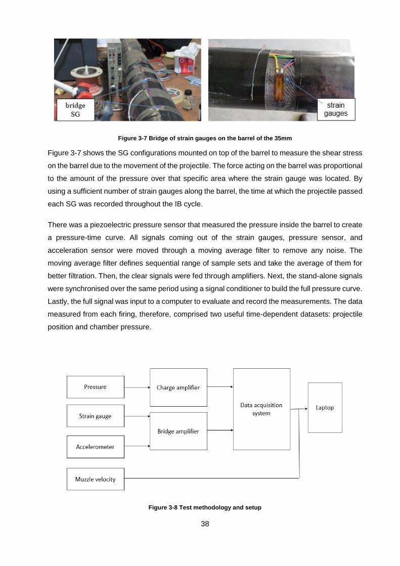
38
Figure 3-7 Bridge of strain gauges on the barrel of the 35mm
Figure 3-7 shows the SG configurations mounted on top of the barrel to measure the shear stress
on the barrel due to the movement of the projectile. The force acting on the barrel was proportional
to the amount of the pressure over that specific area where the strain gauge was located. By
using a sufficient number of strain gauges along the barrel, the time at which the projectile passed
each SG was recorded throughout the IB cycle.
There was a piezoelectric pressure sensor that measured the pressure inside the barrel to create
a pressure-time curve. All signals coming out of the strain gauges, pressure sensor, and
acceleration sensor were moved through a moving average filter to remove any noise. The
moving average filter defines sequential range of sample sets and take the average of them for
better filtration. Then, the clear signals were fed through amplifiers. Next, the stand-alone signals
were synchronised over the same period using a signal conditioner to build the full pressure curve.
Lastly, the full signal was input to a computer to evaluate and record the measurements. The data
measured from each firing, therefore, comprised two useful time-dependent datasets: projectile
position and chamber pressure.
Figure 3-8 Test methodology and setup

39
Figure 3-8 shows both the accelerometer and strain gauges connected to bridge amplifiers for
signal conditioning. The data from the accelerometer was not used for any analysis purposes.
The pressure transducer that was used to measure chamber pressure required a charge amplifier
for signal processing. The pressure transducer was mounted directly into the barrel, and the cases
were drilled to allow the pressure to be measured.
The test weapon had a contact that closed once the trigger was pulled; this contact was used to
measure T0. Radar was used to measure the muzzle velocity of the projectile. A calibrator was
used to check the calibration settings for the charge amplifier and data acquisition system. Data
acquisition of the signals was accomplished with a PicoScope 4424 data acquisition system
connected to a laptop computer. Pico3424 software on the laptop captures and stored the
unfiltered data at various sampling rates. MATLAB was used to further analyse the data.
The following data were recorded for each of the firings:
Muzzle velocity of the projectile – measured by the radar placed next to the weapon
Projectile velocity/displacement – measured by using data from strain gauges
Acceleration of the barrel – measured but not used
Pressure – measured by the piezoelectric transducer
3.6 Firing Trail
The firing trial was performed under the supervision of a specialist, and all the approval
documentation was obtained by the department of shooting range area. All safety aspects were
taken into consideration before and during the experiment. In the case of the firing trail, a projectile
was fired from the 35mm cannon. The tests were conducted at a proofing test range at
Rheinmetall Denel Munition (Somerset West). Five shots were fired during the test with different
propellant masses. The table below shows the particular propellant mass for each shot.
Table 3-2 Propellant mass in each shot
Shot Number Mass Charge (g)
1 270
2 270
3 290
4 315
5 250

40
The used sampling rate was 20 MHz (50 ns sampling time) as this was the highest sampling rate
could be accomplished with the channel count. In order to check that it was within the Nyquist
frequency, the expected time that would take a projectile to travel the shortest distance between
strain gauges has been calculated based on a muzzle velocity (MV) of 1200 m/s:
𝑑3−4 = 0.568𝑚
𝑡3−4 = 𝑑3−4
𝑀𝑉
𝑡3−4 = 473𝑚𝑠
where; d= distance, t= time, MV= Muzzle Velocity
Therefore, the sampling was almost 9500 times faster than this time and were confident that it
would be able to accurately capture the event. Also, capturing strains that resulted from the
excitation of the barrel as these would be orders of magnitude smaller that the strain caused by
the bullet was not the concern.
3.7 Practical Test Instrumentation Limitation
Below is the summary of the instrumentation limitation of the practical test:
The distance between the strain gauges was taken into consideration because of the
attenuations that can be produced by signal interference. The projectile moved too fast
between two strain gauges, leaving insufficient time for the next strain gauge to detect the
signal.
The locations where the strain gauges could be mounted were limited because there are
positions along the gun where there was no possible direct contact between the barrel
and a sensor.
Because of the nature of the projectile resistance curve, the most significant interaction
was during the first 10% of movement; however, that where it is most difficult to access
strain.
The number of available data capturing channels was limited.

41
3.8 Chapter Summary
Chapter 3 provided insights to understand and overcome problems in the current modelling
system. Projectile behaviour, methods of measuring projectile motion, the strain gauge sensor
system, and test limitations were discussed. The test layout for the experiment was presented,
along with rationality for the choice in sensor type. Finally, this chapter provided the sensor
features and elaborated on the expected results.

42
CHAPTER 4 RESULTS
4.1 Introduction
The purpose of this chapter is to presents the results obtained from the experimental tests. The
objective of the tests was to investigate the relationship between pressure, time, and SG
measurements at different shots. The experiments were performed successfully, and the results
are presented in this chapter in detail.
4.2 Test Setup
The experiments were accomplished under the following conditions:
Weighing and loading of 35mm ammunition
Propellant – S350 Final Lot 059/B/2018
Bulk density – 983 g/dm3
Receiver type – OERLIKON KV353 Nr.23 Barrel Nr. Oerlikon-020
Barrel length – 3250 mm
Top charge – 315 g
Middle charge – 290 g
Low charge – 270 g
4.3 Tests Results
The behaviour and the movement of the projectile and the challenges that face the projectile
inside the barrel were investigated during the experiment. In all shots, the pressure and time were
measured at different SG locations. Maximum pressure for each shot was recorded at SG1. Then,
the pressure slightly decreased at SG2 and continued decreasing to the lowest value at SG4.
It was observed that the projectile was affected by the friction and engraving processes due to
the contact between the projectile and the groove and lands of the rifled barrel. The influence of
the friction at the initial movement of the projectile was significant. As the projectile travelled
through the barrel, the effect of the friction decreased and, therefore, the pressure decreased.
The experiment was successful and matched the expected result. The friction and engraving
processes influenced the pressure measurements, as predicted.

43
4.3.1 Shot Number 1 Results
Figure 4-1 illustrates the measurements of the strain gauges and pressure transducer for shot
number 1. The pressure curve represents the breech pressure. The spikes in the strain gauge
curves indicate the time when the projectile passes the corresponding strain gauge.
Figure 4-1 Shot Number 1 results

44
4.3.2 Shot Number 2 Results
Figure 4-2 illustrates the measurements of the strain gauges and the pressure transducer for shot
number 2. The pressure curve represents the breech pressure. The spike of the strain gauges
indicates the time when the projectile passes them.
Figure 4-2 Shot Number 2 results
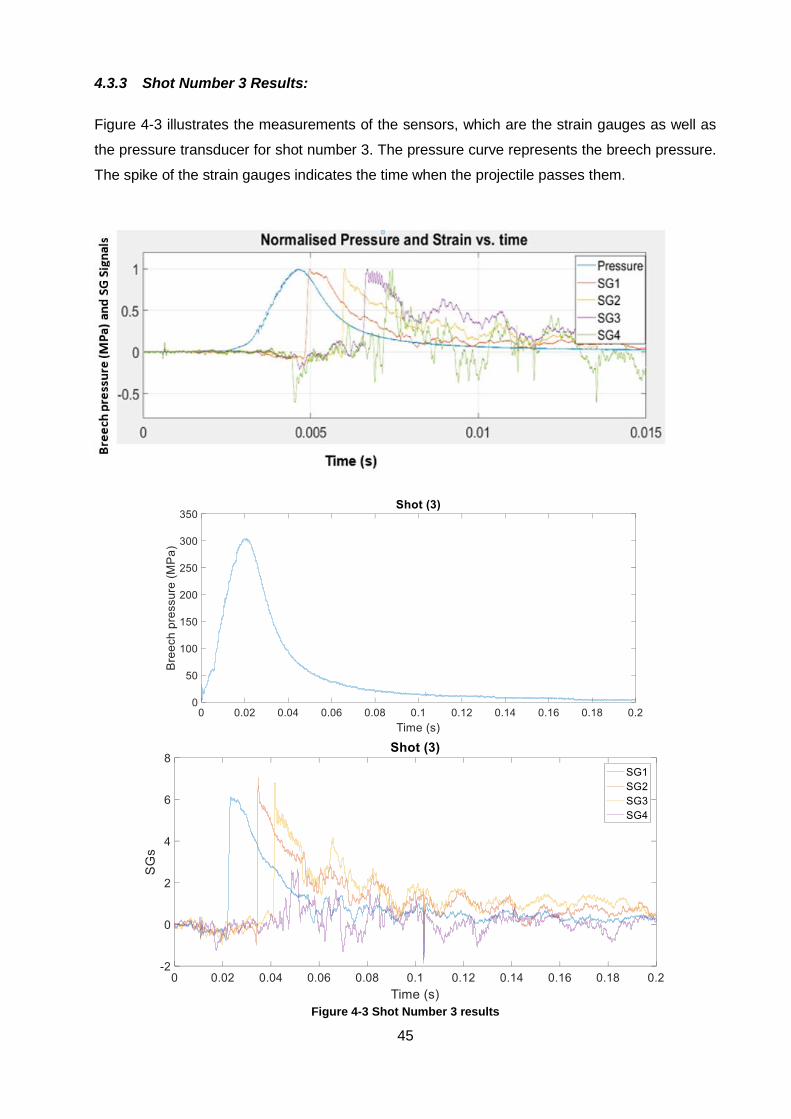
45
4.3.3 Shot Number 3 Results:
Figure 4-3 illustrates the measurements of the sensors, which are the strain gauges as well as
the pressure transducer for shot number 3. The pressure curve represents the breech pressure.
The spike of the strain gauges indicates the time when the projectile passes them.
Figure 4-3 Shot Number 3 results

46
4.3.4 Shot Number 4 Results
Figure 4-4 illustrates the measurements of the strain gauges and the pressure transducer for shot
number 4. The pressure curve represents the breech pressure. The spike of the strain gauges
indicates the time when the projectile passes them.
Figure 4-4 Shot Number 4 results
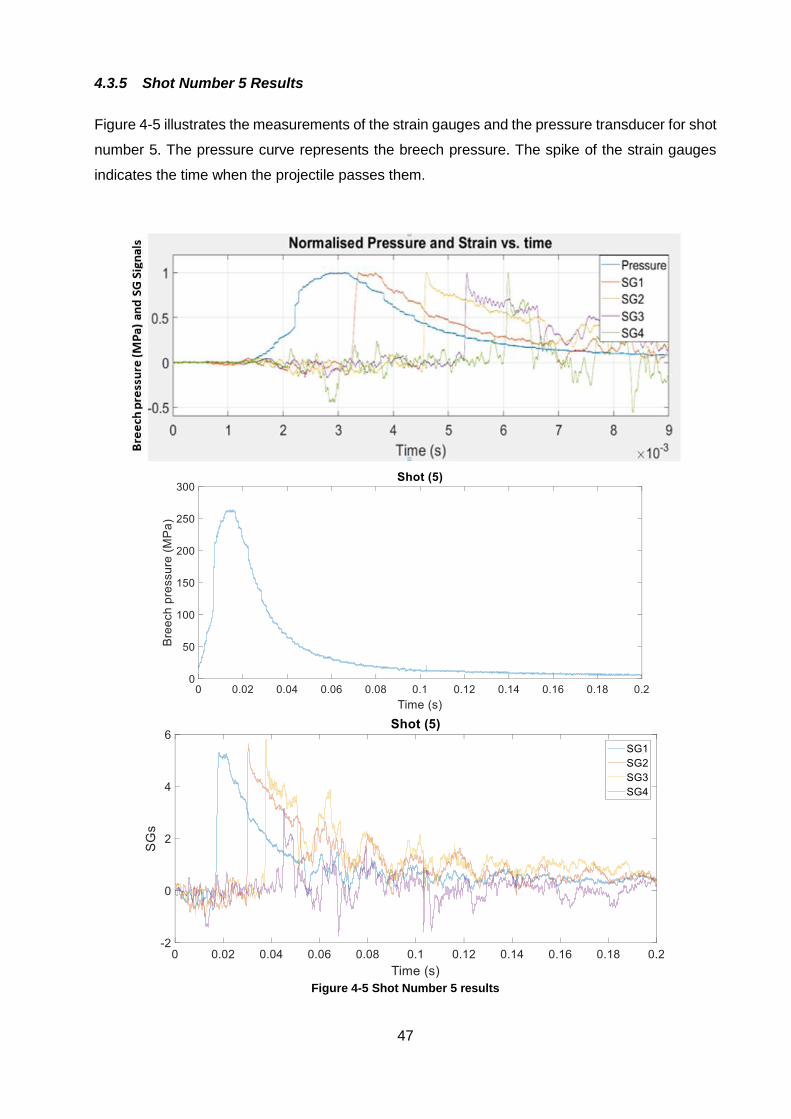
47
4.3.5 Shot Number 5 Results
Figure 4-5 illustrates the measurements of the strain gauges and the pressure transducer for shot
number 5. The pressure curve represents the breech pressure. The spike of the strain gauges
indicates the time when the projectile passes them.
Figure 4-5 Shot Number 5 results

48
Measuring data within such a short duration is difficult. Therefore, multiple attempts were
conducted to obtain accurate measurements. All attempts yielded suitable data since there were
no discontinuities or meaningless oscillations. However, the most accurate data was considered
to be from shot number 4, which exhibited the least amount of noise in the signals. Therefore,
data from shot number 4 were analysed, as shown in Figure 4-6. The corresponding results
algorithm is displayed in the appendix.
Figure 4-6 Breech Pressure and SGs vs time for shot number 4
Figure 4-6 shows the time the projectile passes each strain gauge and the value of the breech
pressure at that moment. This information was the core of this testing since these measurements
were then processed with IB simulation model to obtain the proper resistive curve to calibrate the
IB model.
4.4 Test summary
Table 4-1 presents the results of the measurements at different shots which shows different time
periods of the SGs for different charge masses.
Table 4-1 Results of the measurements at different shots
Shot
number
Muzzle velocity (m/s)
Pressure
(MPa)
Acceleration (g)
Delta t
SG1–SG2
(ms)
Delta t
SG2–SG3 (ms)
Delta t
(SG3–SG4 (ms)
Mass of Charge (g)
1 1025.69 247 2000 1,236 0,724 0,750 270
2 1035.00 257 1140 1,231 0,730 0,730 270
3 1089.29 305 2000 1,147 0,687 0,688 290
4 1171.12 397 400 1,044 0,638 0,627 315
5 1016.18 263 2000 1,222 0,744 0,747 250

49
4.5 Chapter summary
Chapter 4 provided insights into the results obtained from the experimental tests. The projectile
behaviour and the effect of the friction at the initial and final movements through the barrel were
analysed. The maximum pressure was observed at the SG1 for each test. Then, the pressure
value reduces gradually recording the lowest value at SG4. It was observed that the projectile is
affected by the friction and engraving processes due to the contact between the projectile and the
groove and lands of the rifled barrel. Finally, it was determined that shot number 4 data was the
most accurate data and can then be used in the model.

50
CHAPTER 5 DATA ANALYSIS AND PROCESSING
5.1 Introduction
The tests were conducted at the proofing test range at Rheinmetall Denel Munition, and the
results presented in the previous chapter. A 35mm artillery system was used in the experiment,
which during which the behaviour of the projectile inside the barrel due to driving band material
and the engraving process was studied. The test results were analysed using a MATLAB program
to process real data, simulate the result, and investigate variable parameters.
The test results were evaluated to derive a relationship that defines the characteristic resistance
curve for the specific gun system based on the following:
Gun barrel movement at shot start
Pressure of the gun chamber as a function of time
Position of the projectile’s drive band as a function of time
Muzzle velocity (projectile exit velocity)
The above data were utilised to derive the actual projectile resistance as a function of position in
the gun’s barrel. Testing devices and measuring tools used were carefully selected and calibrated
with respect to international standards to avoid any errors during the testing process and to limit
any discrepancies in the results.
Pico3424 software was used to capture and store the unfiltered data at various sampling rates.
MATLAB was used to further analyse the data. As mentioned previously, the shot 4 dataset was
chosen for full data analysis since it had the least noise in the signals.
In this section, experimental findings are discussed and compared to what was expected. The
data, processing, and iteration principles are discussed in detail in this section. Finally, the
limitation of the experimental data and improvements for future work are stated.
5.2 Data Analysis
All the data and relevant variables were initialised for the shot being processed. The shot start
pressure from the accelerometer measurement data was determined, as shown in Figure 5-1, by
inspecting the pressure and integrated acceleration curves. All datasets and relevant variables
were isolated for the shot being processed. The exit pressure can also be investigated by
inspecting the integrated acceleration. As soon as maximum recoil velocity is reached, this implies
barrel exit (~50 MPa), as displayed in Figure 5-1.

51
Figure 5-1 Determination of shot exit pressure
The integrated value of acceleration was plotted with the pressure, and pressure at the maximum
recoil velocity was determined, as shown in Figure 5-1. The data after the exit pressure was
discarded. The strain gauge times were used in the initial calculations of projectile velocity and
translation, which were expected to be higher than the actual values since the resistive pressures
were not yet included. This initial calculation provided an indication of whether the data reduction
process so far was valid.
The resistive pressures and the gas pressure in front of the projectile were considered. The actual
resistance pressures at the SG positions, based on the time the projectile reaches the SG
position, was determined through a multistep iterative procedure, i.e. an iterative calculation for
each strain gauge, as shown in Figure 5-2.
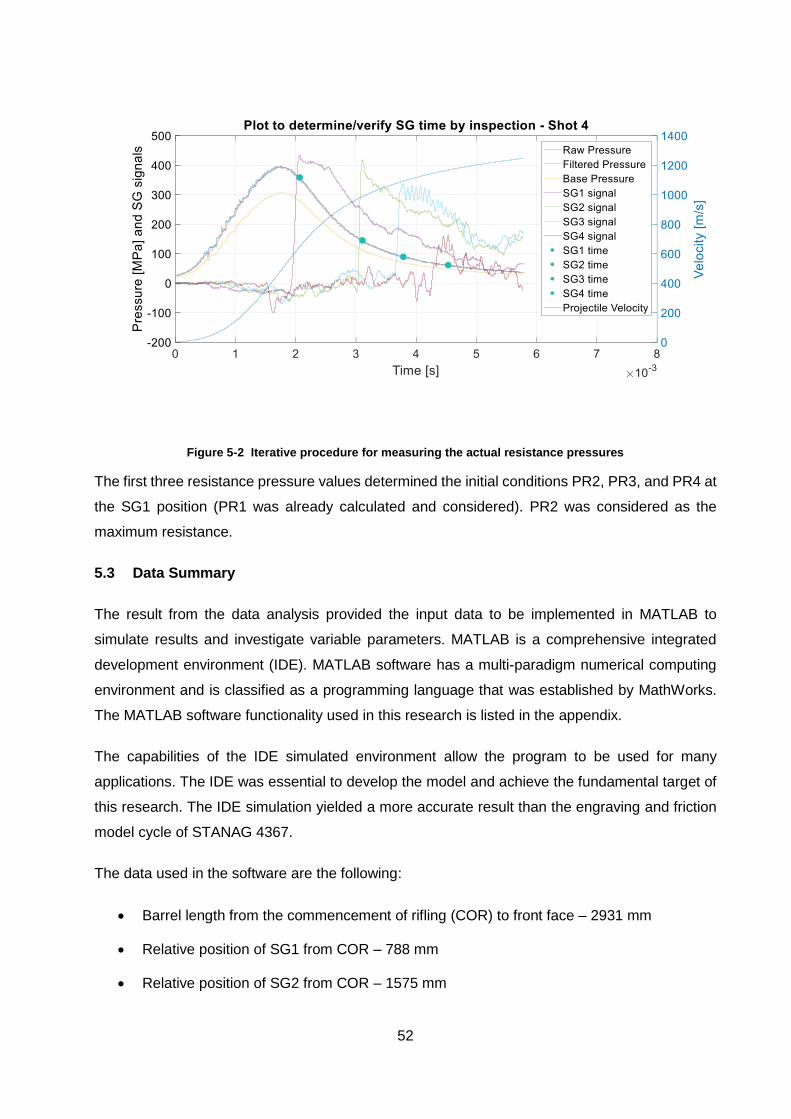
52
Figure 5-2 Iterative procedure for measuring the actual resistance pressures
The first three resistance pressure values determined the initial conditions PR2, PR3, and PR4 at
the SG1 position (PR1 was already calculated and considered). PR2 was considered as the
maximum resistance.
5.3 Data Summary
The result from the data analysis provided the input data to be implemented in MATLAB to
simulate results and investigate variable parameters. MATLAB is a comprehensive integrated
development environment (IDE). MATLAB software has a multi-paradigm numerical computing
environment and is classified as a programming language that was established by MathWorks.
The MATLAB software functionality used in this research is listed in the appendix.
The capabilities of the IDE simulated environment allow the program to be used for many
applications. The IDE was essential to develop the model and achieve the fundamental target of
this research. The IDE simulation yielded a more accurate result than the engraving and friction
model cycle of STANAG 4367.
The data used in the software are the following:
Barrel length from the commencement of rifling (COR) to front face – 2931 mm
Relative position of SG1 from COR – 788 mm
Relative position of SG2 from COR – 1575 mm

53
Relative position of SG3 from COR – 2363 mm
Relative position of SG4 from COR – 2931 mm
Mass of propellant – 315 g
Mass of projectile – 550 g
Pressure (Max) – 397 MPa
Velocity – 1171 m/s
Barrel groove diameter – 35.1 mm
Land diameter – 35 mm
Land-to-groove ratio – 1.1
5.4 Model Construction
Scientists in ballistic fields use data analysis algorithms to analyse the behaviour of the projectile,
determine the optimum parameters, and make predictions by applying mathematical code
describing the interior ballistic cycle. These algorithms also help address the lack of information
within the internal ballistic system.
The model data analysis algorithms are used to solve a specific problem using mathematical
codes. STANAG equations for pressures and projectile travel were used to build a model that
calculates the position of the projectile at a given time for each strain gauge (from strain gauge
measurements). Applying the equations listed in Chapter 2, MATLAB software was used to
compile the data analysis code. The general sequence of the MATLAB code was as follows:
1. Input Data – All input data, including that of the igniter and propellant, were analysed using
various parameters]. These data are necessary to determine the gas constant, heat
capacities, and others.
2. Initialisation – The input data were initialised to set values, e.g. derivatives and state vector
at zero time t0.
3. Calculation of IB cycle – Integrated parameters were assigned to obtain suitable variables,
such as distance, recoil distance, velocity, the energy loss of air displacement, the energy
of heat transfer, propellant distance, the mass fraction of propellant gas based on burn
distance, total burn, the average remaining propellant volume and gas properties, kinetic
energy of projectile and gas/propellant, projectile rotational velocity and energy, F\friction
energy, gas temperature, an average of the chamber pressure, breech and base
pressures, burn rates of propellant, projectile acceleration based on base pressure, and
recoil acceleration based on breech pressure. All the parameters were integrated over

54
time to the endpoint where the projectile reached the barrel. IB model calculations were
then terminated.
4. Output array: distance, acceleration, time, velocity, and average pressure (Brinson &
Brinson, 2015).
During the analysis, the sequence of MATLAB code was as follows:
1. Initialise all data sets and relevant variables for the shot being processed. The
experimental data was imported and allocated to variables for processing.
2. Determine the shot start pressure from the accelerometer measurement data. The plot is
used to determine shot start pressure by inspecting the pressure and integrated
acceleration curves.
3. Process the data. Only relevant data was prepared for display.
The shot start pressure was estimated based on the plot of the integrated acceleration curve. The
relevant datasets from the shot start onwards were isolated. The exit pressure was also
determined by inspecting the integrated acceleration. The maximum recoil velocity implies the
moment of barrel exit (~50 MPa). The integrated value of acceleration (i.e. velocity) was plotted
with the pressure, and the pressure at the maximum recoil velocity was determined. All data after
the exit pressure was discarded.
The strain gauge times were determined in the following step. The boundary effect was then
removed, and all the other datasets were followed the same procedure. The data was isolated
further and discarded all other data after the projectile. Now, the pressure data was filtered, and
the time and pressure index of strain gauges were determined where projectile passes. Then,
time and pressure for each strain gauge were recorded. Now, the time and pressure were
extracted when each strain gauge reflects the projectile moving passed.
The base pressure based on the Lagrange gradient model was then calculated, as introduced in
Chapter 2. The raw, base, and filtered pressures were plotted. Also, amplified strain gauge signals
were plotted on the same graph for visualisation. The position on the pressure curve for each
strain gauge activation by a projectile was marked. The initial nominal calculated velocity was
plotted on the secondary axis. The next step was to consider the resistive pressures and the gas
pressure in front of the projectile, as mentioned in Chapter 2.
The actual resistance pressures PR at the SG positions were determined based on the time the
projectile reached the SG, which required a multistep iterative procedure for each strain gauge.
The first three resistance values were estimated as initial conditions, which were PR2, PR3 and
PR4 (SG1 position), where PR1 was already calculated.

55
For procedure step 1, the value and iterate PR4 (SG1 position) resistance value was estimated.
Then, the value and iterate until PR2-4 were calculated. Finally, the value and iterate until SG1
time were to matched calculation.
In procedure step 2, the PR5 (SG2 position) resistance value was determined and adjusted in an
iteration. The iterate until SG2 time was matched to the calculation.
In the case of procedure step 3, PR6 (SG3 position) resistance value was determined and
adjusted in iterate until SG3 time was matched to the calculation.
For procedure step 4, PR7 (SG4 position) resistance value was determined and adjusted in
iteration until SG4 time was matched to the calculation. At this point, all the PR values are now
solved.
In procedure step 5, the calculation with a complete cycle integration using the calculated PR
values was verified. Therefore, the calculated velocity is measured as additional have more
verification.
Procedure step 6 used the simulation and calibration to verify the results. All the equations are
provided in the appendix.

56
Figure 5-3 Flow chart plan for the IB model
From Figure 5-3, the input data are assigned and then initialised to set different variables at zero
time t0. There are eight points along the barrel assessed in the calculation, including the four strain
gauge locations. All the integrated data of the IB model for SG1 were assigned to obtain suitable
variables. If the projectile transition aligned with the measured data, the integrated data were
submitted to the IB model for SG2. Otherwise, the Pr value was adjusted, and then the IB model
was rerun for SG1. Similar procedures were followed to run the IB model for SG2, SG3, and SG4.
Finally, the output data were posted, and the IB model was terminated.

57
5.5 Model Verification
After developing the interior ballistic model from this research, it required verification against the
interior ballistic simulation program of RDM, which is STANAG 4367 compliant. The RDM IB
model has been in service for almost 20 years. Throughout these years, the interior ballistic
simulation program of RDM has been continuously improved, verified, and validated and is
extensively utilised in product development. It has been tested against hundreds of ballistic
systems from small, medium, and large calibre systems (used for 35mm calibre simulation).
Table 5-1 shows the outputs generated by the developed IB model versus that of the RDM IB
model using the same inputs. Despite the relatively large deviation between the outputs of the
two models, the results of the developed model were closer to the measured data. As a result,
the developed IB model was verified.
Table 5-1 RDM IB model vs Developed Model
35mm System RDM Developed program
Maximum Pressure (MPa) 378.3 331.3
Muzzle Velocity (m/s) 917.1 969.7
5.6 Results of the Semi-empirical Resistive Pressure Curve of 35mm Cannon
By following the data analysis principles, the method worked successfully. Ballistic verification
aligned with the measured values. The factor for adjusting the base pressure was introduced.

58
Figure 5-4 Showing the semi-empirical resistive pressure curve of 35mm cannon
The semi-empirical resistive pressure curve of the 35mm cannon is shown in Figure 5-4. The
friction model was used to adjust the data to realistic values and calculate the maximum engraving
pressure and velocity during the interior ballistic cycle.
The graph contains eight points in the calculation, including four strain gauges as follows:
Point one (P1) is shot start pressure point and shows the resistance pressure before the
movement of the projectile.
Points two and three (P2 and P3) are assigned when the projectile begins to travel through
the barrel. The two points between the shot start pressure point and point four (SG1
position) are calculated during the solution from shot start pressure point to SG1 position.
The two points are used to predict the resistance values between the shot start pressure
point and the SG1 position. This is the area where the pressure peaks owing to the
engraving and friction processes.
The following points five (P5), six (P6), and seven (P7) correspond to the SG2, SG3, and SG4 positions, respectively.
Finally, Point eight (P8) represents the barrel exit.
Barrel Length (m)

59
The results are summarised in Table 5-2.
Table 5-2 The semi-empirical resistive pressure at different time intervals
Points 1 2 3 4 5 6 7 8
PR (MPa) 0.043 15 66 33 2.5 1.3 8.4 0.68
Projectile displacement (m)
0.000 0.010 0.020 0.788 1.575 2.363 2.931 3.330
5.7 Implementation of the Semi-Empirical Resistive Pressure Curve of 35mm Cannon
into the Developed Model
The following Figure 5-5 shows the semi-empirical resistive pressure curve, which was applied in
the developed IB model. The semi-empirical resistive curve of the cannon consists of eight points,
unlike the classical one, which consists of four points. In other words, the more points to measure
the pressure the more accurate the results are.
Figure 5-5 The semi-empirical resistive curve of the 35mm cannon
Table 5-3 shows the result of the developed IB model before and after implementing the resistive
semi-empirical resistive pressure curve of 35mm cannon. There is no difference in maximum
pressure predicted. The muzzle velocity only shows a slight increase of 0.15 m/s.
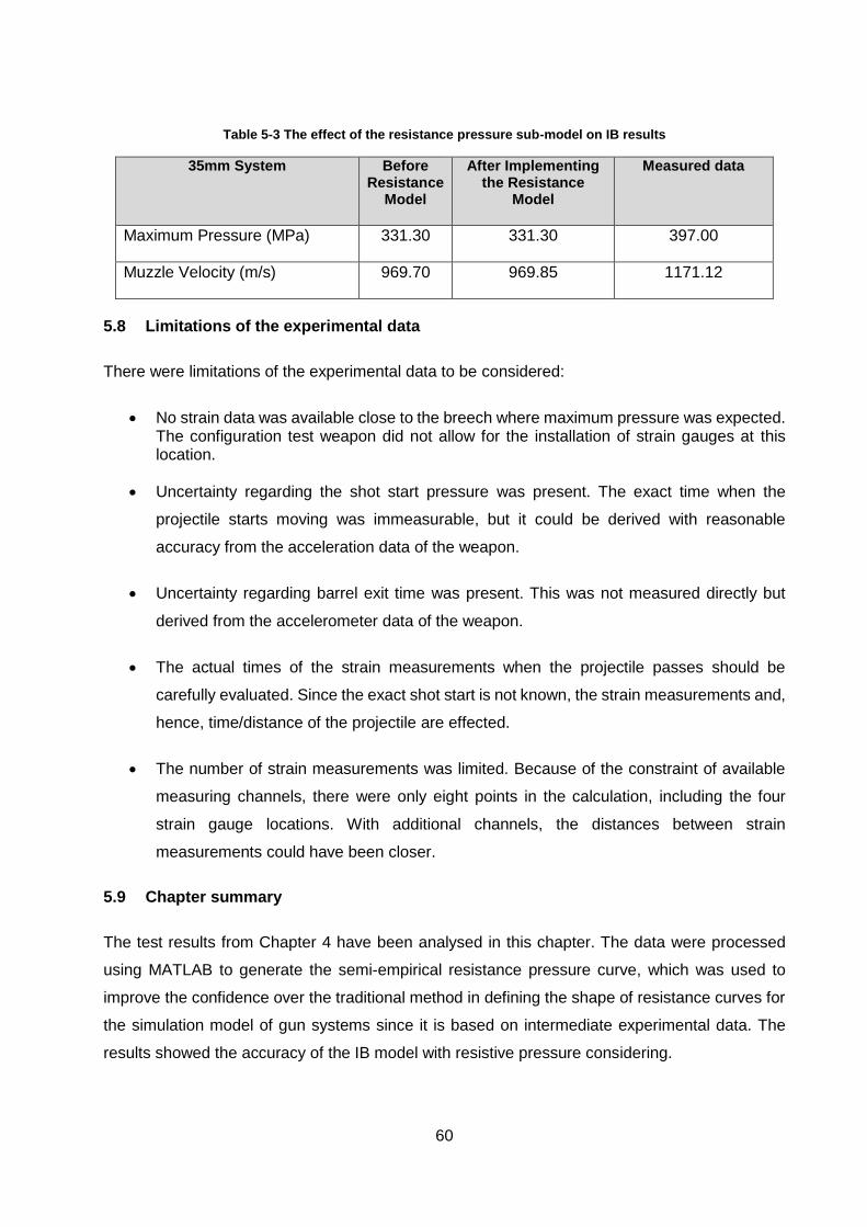
60
Table 5-3 The effect of the resistance pressure sub-model on IB results
35mm System Before Resistance
Model
After Implementing the Resistance
Model
Measured data
Maximum Pressure (MPa) 331.30 331.30 397.00
Muzzle Velocity (m/s) 969.70 969.85 1171.12
5.8 Limitations of the experimental data
There were limitations of the experimental data to be considered:
No strain data was available close to the breech where maximum pressure was expected. The configuration test weapon did not allow for the installation of strain gauges at this location.
Uncertainty regarding the shot start pressure was present. The exact time when the
projectile starts moving was immeasurable, but it could be derived with reasonable
accuracy from the acceleration data of the weapon.
Uncertainty regarding barrel exit time was present. This was not measured directly but
derived from the accelerometer data of the weapon.
The actual times of the strain measurements when the projectile passes should be
carefully evaluated. Since the exact shot start is not known, the strain measurements and,
hence, time/distance of the projectile are effected.
The number of strain measurements was limited. Because of the constraint of available
measuring channels, there were only eight points in the calculation, including the four
strain gauge locations. With additional channels, the distances between strain
measurements could have been closer.
5.9 Chapter summary
The test results from Chapter 4 have been analysed in this chapter. The data were processed
using MATLAB to generate the semi-empirical resistance pressure curve, which was used to
improve the confidence over the traditional method in defining the shape of resistance curves for
the simulation model of gun systems since it is based on intermediate experimental data. The
results showed the accuracy of the IB model with resistive pressure considering.

61
CHAPTER 6 CONCLUSION
6.1 Research Overview
This dissertation examined the implementation of the resistive pressure sub-model to enhance
the accuracy of the overall IB model. The approach was to develop a test setup to gather
information necessary to realise the resistance curve that is characterised by different firing
conditions.
Chapter 1 – This chapter gave a detailed introduction to the gun system. Current problems facing
internal ballisticians were presented. The research methodology was also outlined.
Chapter 2 – This chapter presented a review of existing literature and the latest developments
concerning resistance models of internal ballistics systems. Available scholarly work in the field
of internal ballistics was highlighted, and various concepts explaining the internal ballistic system
were presented.
Chapter 3 – This chapter dealt with the methodology of the experiment, safety precaution,
weapon system and setup, gun preparation, strain gauge installation, firing trail, practical test
instrumentation limitation, and test layout for the experiment.
Chapter 4 – This chapter described the result obtained from the experimental tests. The result of
the experiments showed the relationship between pressure, time, and variable SGs at different
shots. The results were then displayed.
Chapter 5 – This chapter described the data analysis and processing of the IB model simulated
by MATLAB software. The data summary and the results of the semi-empirical resistive pressure
curve were presented showing the adequacy of resistive curve implementation to the IB model.
6.2 Conclusion
This study developed a semi-empirical barrel engraving resistance test method for internal
ballistic simulation codes. The aim of this study was to determine the characteristic pressure
resistance curve via the stated intermediate approach through internal ballistic simulation using
experimental data from live firings. The objectives in this study were to a) establish a test platform
for measuring projectile travel and relevant ballistic parameters during live firings, b) develop a
method and related software tools to analyse the measured data and derive a resistance curve
for the ballistic system, c) obtain suitable data from live firing conducted from a series of
experiments, which then could be utilised to derive resistance curves to be implemented in an

62
internal ballistic simulation model, and d) demonstrate the implementation of such a resistance
model in comparison to the traditional empirical model.
The experiments were conducted successfully, and the required results were obtained, as
presented in the previous chapter. The measured data was processed and modelled to derive the
semi-empirical resistive curve of the 35mm cannon. After that, the IB model is developed and
verified against RDM’s IB model. Finally, the semi-empirical resistance curve was implemented
into the developed IB model, and the result was compared to the result of the IB model before
implementing the semi-empirical resistance curve with the measured data.
The difference between the simulation result before and after implementing the semi-empirical
resistance curve did not significantly vary. The maximum pressure showed no changes whereas
the muzzle velocity showed a slight difference by 0.15 m/s. This unchanging model results is
because of the following reason. The strain gauges were placed after the real engraving
phenomenon, which occurs at the beginning of the barrel. In this study’s strain gauge placement,
the driving band was already worn out by the time the projectile passes the strain gauges. As a
result, the friction that the projectile is subjected to is minimal, which might have minimal effect
on the ballistics of the projectile.
6.3 Future Work
After investigating the interior ballistic cycle and obtaining the results mentioned above, some
improvements are proposed for future work:
Shot start pressure measurement by an alternative method. The exact time the projectile
starts moving needs to be measured to accurately determine the pressure at which this
occurs. Possible solutions include a broken wire or contact screen in the barrel.
Accurate measurement of exit time to determine exit pressure. A contact screen, broken
wire, or pressure gauge could be used to measure the exact time of barrel exit.
Additional strain gauges between the shot start and maximum pressure, if possible (100–
200mm from COR). This would provide essential information to the pressure resistance
model.
Continuous displacement measurements. A promising solution could be to use a wire
fitted to the front of the projectile and isolating it from the barrel. The resistance of this
circuit can then be measured as it changes as the projectile moves through the barrel.
This measurement can address several problems, including the challenges at the shot
start and barrel exit.

63
BIBLIOGRAPHY
Bougamra, A., & Lu, H. (2014). Multiphase CFD simulation of solid propellant combustion in a
small gun chamber. International Journal of Chemical Engineering, v2014 (2014 01 01):.
Brinson, H. F., & Brinson, L. C. (2015). Polymer Engineering Science and Viscoelasticity : an
Introduction. New York: Springer.
Carlucci, D. E., & Jacobson, S. S. (2018). Ballistics : Theory and Design of Guns and
Ammunition, Third Edition. Boca Raton, FL : CRC Press.
Crowley, A. B. (1999, November). Effect on barrel wear on weapon performance. the 21st
International Symposium on Ballistics , 228-235.
Deng, S., Sun, H. K., Chiu, C.-J., & Chen, K.-C. (2014). Transient finite element for in-bore
analysis of 9 mm pistols. Applied Mathematical Modelling, v38 n9-10 (201405): 2673-
2688.
Dyckmans, G. (2015). Energy Balance. e-ballistics. Retrieved from Retrieved from https://e-
ballistics.com/ebook/internal ballistics - energy balance.htm#GasInertia
Gray, E., Marsh, H., & McLaren, M. (1982). A short history of gunpowder and the role of
charcoal in its manufacture. Journal of Materials Science, 17(12), 3385-3400.
Gunpowder. (2019, 03 1). Retrieved from Wikipedia, the free encyclopedia. Retrieved from:
https://en.wikipedia.org/wiki/Gunpowder
Hansen, E. C., & Heiney, O. K. (n.d.). Pressure and gas flow gradients behind the projectile
during the interior ballistic cycle. ; University of Florida. Department of Mechanial
Engineering: Canoga Park, CA : Rockwell Intl Corp., 1987.
Kelly, J. (2004). Gunpowder : Alchemy, Bombards, and Pyrotechnics - The History of the
Explosive That Changed the World. New York : Basic Books, 2009.
Kirchner, D. B. (1993). Combustion products of propellants and ammunition. Occupational
health–the soldier and the industrial bas. Falls Church, Va. : Office of the Surgeon
General, U.S. Dept. of the Army ; Aberdeen Proving Grounds, Md. : U.S. Army
Environmental Hygiene Agency ; Bethesda, Md. : Uniformed Services University of the
Health Sciences ; Washington, DC : For sale by the S.

64
Koffler. (2015). Rifled Barrel vs Smooth Barrel. Retrieved from Retrieved from
https://rivervalleyarms.com/2015/11/07/slug-country-debates-rifled-barrel-versus-
smooth-bore/
Kubota, N., & VCH-Verlagsgesellschaft. (2015). Propellants and explosives : thermochemical
aspects of combustion. John Wiley & Sons.
Moreno, J. A. (2009). Thermodynamic Interior Ballistic Model With Global Parameters.
Retrieved from. NATO.
Morrison, W. F., Wren, G. P., Oberle, W. F., & Richardson, S. L. (1993). The Application of
Lagrange and Pidduck-Kent Gradient Models to Guns Using Low Molecular Weight
Gases. Ft. Belvoir Defense Technical Information Center FEB 1993.
Okunev, B. O. (1943). ballistiki [Fundamentals of Ballistics]. Voenizdat, . . Moscow.
Quanzhao, S. G. (2017). Modeling and simulation on engraving process of projectile rotating
band under different charge cases. Journal of Vibration and Control, 23, 6,, 1044-1054.
Ruge, A. (1944). US Patent No. 2,350,97.
Sättler, A. P. (2013). Investigation of the Projectile Movement Inside a Gun Tube Using a
Photonic Doppler Velocimeter. (pp. 50-58).
Schabort. (2016). RDM Internal Ballistic Course. RDM. Somerset West.: 2016.
STANAG 4367. (2012). THERMODYNAMIC INTERIOR BALLISTIC MODEL WITH GLOBAL
PARAMETERS 4367. NATO.
Worsfold, P., Townshend, A., Poole, C. F., & Miro, M. (2019.). Encyclopedia of analytical
science. Amsterdam : : Elsevier,.
Xue, T., Zhang, X.-b., & Cui, D.-h. (2014). Dynamic analysis of a guided projectile during
engraving process. Defence Technology, v10 n2 (201406):, 111-118.

65
ANNEXURES
Code - Data analysis
clear all;
close all;
clc;
% I WILL DO SOME AUTOMATION HERE - FRAMEWORK TO BE ESTABLISHED
%Step1
%Step2
%Step3
%Iteration Step1
%Iteration Step2
%Iteration Step3
%Iteration Step4
%Verification
%Simulation
%% Shot 4 Summary:
% Barrel length from COR (commencement of rifling) to front face: 2931 mm ??
% Relative Position of SG1 (Strain guage 1) from COR: 788 mm
% Relative Position of SG2 (Strain guage 2) from COR: 1575 mm
% Relative Position of SG3 (Strain guage 3) from COR: 2363 mm
% Relative Position of SG4 (Strain guage 4) from COR: 2931 mm
% Mass of propellant = 315 g
% Mass of projectile = 550 g
% Pressure (Max) = 1171 [m/s]
% Velocity = 397 [MPa]
% Barrel Groove Diameter = 35.1 mm
% Land Diameter = 35 mm
% Land to Groove ratio = 1.1

66
%
%% First Step is to Initialize all data sets and relevant variables for the
Shot being processed
%
%
%
dt = 5e-08; % Time step size [s] from Sampling rate
WindowSize = 500; % Filter window size
X = 1:WindowSize; % create filter function
Filter = 1/sum(sin(pi*X/WindowSize))*sin(pi*X/WindowSize); % Moving average
filter window based on die function
LandDiam = 0.035; % mm
GrooveDiam = 0.0351; % mm
LndGrvratio = 1.1;
ProjMass = 0.550; % Projectile Mass [kg]
PropellantMass = 0.315; % Propellant Mass [kg]
BaseArea = 0.25*pi*GrooveDiam^2; %
Eps = PropellantMass/ProjMass; % See Course notes (Lagrange ratio)
% Import experimental data and allocate to variables for processing
data = importdata('Shot_4.txt');
P = data (:,1); % Pressure
x1 = data (:,2); % ?
SG1 = data (:,3); % Strain Guage 1
SG2 = data(:,4); % Strain Guage 2
x2 = data(:,5); % ?
SG3 = data(:,6); % Strain Guage 1
SG4 = data(:,7); % Strain Guage 1

67
Acc = data(:,8); % Accellerometer
Acc = filter(Filter',1,Acc); % Filtered data
AccInt = cumtrapz(Acc); % Integrate Accelleration to get
velocity (trapezium rule)
%% Next step is to determine the Shot Start Pressure form the accellerometer
measurement data
%
% Use this plot to determine shot start pressure by inspecting the P and
% integrated acceleration curves
[MaxP,MaxIndex] = max(P); % Maximum pressure index
Time = dt*(0:1:(length(P)-1))'; % Time series based on
time step value
figure(1);
plot(Time,P); % Plot pressure time
curve
hold on;
AccInt(MaxIndex+100000:length(AccInt),:) = 0; % Ignore Acc data
after max pressure (we do not need this)
Acc(MaxIndex+100000:length(AccInt),:) = 0;
ylabel("Pressure");
yyaxis right;
plot(Time,Acc*1000,'b:'); % Plot accelleration as
well as velocity vs time
plot(Time,AccInt,'r-');
grid on;
title("Plot to determine Shot Start Presure");
xlabel("Time [s]");
ylabel("Barrel Velocity");
legend('Pressure','Barrel Acc','Barrel V (Integrated Acc)');
%return; % Un-comment this stement
and first confirm the Shot Start Pressure

68
% Shot Start pressure was determined - so we can move on - comment out the
return statement
%% Next Step - Process the data - Isolate only relevant data and prepare for
display on Figure 2
%
% Please follow comments to inspect process
% You can descrive this process in you dissertation
%
ShotStartP = 35.0; % Estimated Shot Start Pressure based on plot 1 -
integrated accelleration curve
for i = 1:(length(P)) % Find the index of the shot start pressure
if P(i) >= ShotStartP % Pressure on the way up
ShotStartIndex = i;
break;
end
end
% Now Isolate relevant data from shot start onwards
P(1:ShotStartIndex,:) = []; % Discard data up to shot start
SG1(1:ShotStartIndex,:) = [];
SG2(1:ShotStartIndex,:) = [];
SG3(1:ShotStartIndex,:) = [];
SG4(1:ShotStartIndex,:) = [];
Acc(1:ShotStartIndex,:) = [];
AccInt(1:ShotStartIndex,:) = [];
Size = length(P);

69
%% Exit pressure can also be determined by inspecting the integrated Acc
% As soon as maximum recoil velocity is reached, this implies barrel exit
% (this is around 50 MPa - you can also include this in ypou dissertation!)
% Simply Plot the integrated value against the pressure, read of the
% pressure against the maximum recoil velocity - This is done in the
% following plot
figure(2);
Time = dt*(0:1:(length(P)-1))'; % Create new Time series
plot(Time,P);
hold on;
plot(Time,AccInt/10000); % You can inspect this graph and
derive exit pressure/time
title('Graph to determine shot exit pressure by inspection');
xlim([0 10/1000]); % Zoom to first 10 milliseconds
[MaxAcc,MaxAccIndex] = max(AccInt);
scatter(Time(MaxAccIndex),P(MaxAccIndex),150,300,'filled');
ExitPressure = P(MaxAccIndex); % This should be adjusted according
to inspection of data (can also be verified by simple velocity calulations)
%return; % Commnet this statment before
moving to the next step
%% Discard of all data after exit pressure
% Get the starin guage times to be used for the next step
%
for i = 10000:(length(P)) % Find the index of the shot exit pressure
if P(i) < ExitPressure % Pressure on the way down
ExitIndex = i;
break;
end

70
end
% Isolate data further
P( ExitIndex:length(P),:) = []; % Discard all data after projectile
exit
SG1(ExitIndex:length(SG1),:) = [];
SG2(ExitIndex:length(SG2),:) = [];
SG3(ExitIndex:length(SG3),:) = [];
SG4(ExitIndex:length(SG4),:) = [];
Acc(ExitIndex:length(Acc),:) = [];
% Now Filter the Pressure Data
PFilt = filter(Filter',1,P); % Filtered pressure
P(1:WindowSize,:) = []; % Discard filter boundary effect
PFilt(1:WindowSize,:) = []; % Remove boundary effect
SG1(1:WindowSize,:) = []; % Do the same for all the other
data sets
SG2(1:WindowSize,:) = [];
SG3(1:WindowSize,:) = [];
SG4(1:WindowSize,:) = [];
Acc(1:WindowSize,:) = [];
Time = dt*(0:1:(length(P)-1))'; % Create new Time series
% Find the time and pressure index of strain gauges where projectile passes
for i=1:length(P)
if(SG1(i)*60 > P(i))
I1 = i;
break;
end
end
for i=1:length(P)
if(SG2(i)*60 > P(i))
I2 = i;

71
break;
end
end
for i=1:length(P)
if(SG3(i)*60 > P(i))
I3 = i;
break;
end
end
for i=1:length(P)
if(SG4(i)*60 > P(i))
I4 = i;
break;
end
end
% Record Time and Pressure for each strain guage
tSG1 = Time(I1); PSG1 = P(I1);
tSG2 = Time(I2); PSG2 = P(I2);
tSG3 = Time(I3); PSG3 = P(I3);
tSG4 = Time(I4); PSG4 = P(I4); % This was extracted by inspection of the
data
tSG = [tSG1 tSG2 tSG3 tSG4]; % Extract the time and Pressure when each
strain gauge reflects the projectile moving passed
PSG = [PSG1 PSG2 PSG3 PSG4]; % And the related pressure
%% Initial calculation of Projectile velocity and translation
% These initial values should be higher than the actual values, since the
% resistive pressures have not been considered yet
% This will provide a good indication whether data reduction process so far
was

72
% sufficiently correct
Pbase = P/(1+Eps/2); % Calculate Base pressure from
from Lagrange
ProjA = (Pbase*1000000)*BaseArea/ProjMass; % Air and Barrel Resistance not
yet considered- First Order calculation to check the data processing
ProjV = cumtrapz(ProjA)*dt;
ProjX = cumtrapz(ProjV)*dt;
% Now create a new Figure and plot all relevant data for visualization and
inspection
figure(3);
plot(Time,P); % Plot raw and filtered pressure and Base pressure
hold on;
plot(Time,PFilt);
plot(Time,Pbase);
plot(Time,SG1*60); % Plot Strain gauge signals on same axis with some
amplification just for visualization
plot(Time,SG2*60);
plot(Time,SG3*60);
plot(Time,SG4*60);
sz = 120;
scatter(tSG1,PSG1,sz,300,'filled'); % Mark position on pressure curve for
each strain guage activation by projectile
scatter(tSG2,PSG2,sz,300,'filled');
scatter(tSG3,PSG3,sz,300,'filled');
scatter(tSG4,PSG4,sz,300,'filled');
xlabel('Time [s]');
ylabel('Pressure [MPa] and SG signals');
yyaxis right; % Plot initial nominal calculated
velocity on the secondary axis
plot(Time,ProjV);
ylabel('Velocity [m/s]');
grid on;

73
title('Resistive Pressure Data analysis - Shot 4');
legend('Raw Pressure','Filtered Pressure','Base Pressure','SG1 signal',...
'SG2 signal','SG3 signal','SG4 signal','SG1 time','SG2 time','SG3
time','SG4 time','Projectile Velocity');
%%
%% The next step is to consider the resistive pressures also as well as the
gas pressure in front of projectile
% The objective is now to calculate the actual resistance pressures at the
% SG positions, based the time the projectile reaches the SG position.
% This will require a multistep iterative procedure -
% i.e. an iterative calculation for each strain guage
% The first three resistance values are guessed as an initial condition -
% That is PR2 PR3 and PR4(SG1 position), PR1 was already calculated
% So:
% Procedure Step 1
% PR1 - Shot Start Pressure (already determined)
% PR2 - Maximum resistance - Iterative calculation 1 - Guess value
and iterate
% PR3 - Second Resistance Pressure - Iterative calculation 1 - Guess value
and iterate
% PR4 - SG1 resistance value - Iterative calculation 1 - Guess value
and iterate - Iterate until PR2-4 is % calculated
% Iterate until SG1 time matched calculation
% Procedure Step 2:
% PR4 - SG2 resistance value - Iterative calculation 2 - Adjust this
value in iteration
% Iterate until SG2 time matched calculation

74
% Procedure Step 3:
% PR4 - SG3 resistance value - Iterative calculation 3 - Adjust this
value in
% Iterate until SG3 time matched calculation
% Procedure Step 4:
% PR4 - SG4 resistance value - Iterative calculation 4 - Adjust this
value in iteration
% Iterate until SG4 time matched calculation
% All the PR value are now solved
% Procedure Step 5: verify the calculation with a complete cycle
% integration using the calculated PR values and verify that calculated
velocity = measured velocity
% Working on this - to follow!!!
% Procedure Step 6: Verify by simulation and calibration
% To follow !!!
%% Save data
% Write extracted Pressure, Time and SG Times to files
fid = fopen('Pressure.txt','wt');
fprintf(fid,'%f\n',P);
fclose(fid);
fid = fopen('SGData.txt','wt');
fprintf(fid,'%f\n',[tSG PSG]);
fclose(fid);

75
Code - Resistance Pressure model
clear all;
%%% data processing
data = importdata('pt.txt');
data1 = importdata('ts.txt');
PRdata = importdata('PR.txt'); % in Pa;
Pbr = data*1000000;
ts = data1;
dt = 5e-08;
t = dt*(0:1:(length(Pbr)-1))';
%%%
global PropGeom; % Gas properties (Input)
PropGeom =
struct('Type',0,'a',0.0,'b',0.0,'c',0.0,'L',0.0,'D',0.0,'P1',0.0,'P2',0.0,'W1
',0.0,'W2',0.0,'SlabW',0.0,'SlabL',...
0.0,'SlabT',0.0,'SlotW',0.0);
global PropChem; % Gas properties (Input)
PropChem =
struct('R',0.0,'Cv',0.0,'Cp',0.0,'Fp',0.0,'CoVol',0.0,'FlamTemp',0.0,'Rho',0.
0,'Gamma',...
0.0,'Mass',0.0,'BurnCoeff',0.0,'BurnExp',0.0);
global XR;
global PR;
%%% initial condition
% Gun Input (35 mm)
ChVolume = 550.0; % Chamber Volume [cc]
ChVolume = ChVolume/1000000.0; % to m3

76
ProjMass = 0.550; % ProjMass[kg]
GrooveLength = 2.931; % [m]
RiflingTwist = 20; % 1x360deg (2pi radians) Rotation in this
number of calibres travel [rad/m]
RecoilMass = 0.0; % Total mass of recoil - in this case the
rifle - free recoil - if mass = 0, recoil is ignored
RecoilResistance0 = 0.0; % Initial threshold recoil resistance [N]
RecoilResistance = 0.0; % Cycle Recoil resistance [N]
GrooveDiam = 0.0351; % [m]
LandDiam = 0.035; % [m]
GLRatio = 1.1; % Ratio of groove width to land width
BarrelDiamSq = LandDiam*GrooveDiam;
ProjBaseArea = 0.25*pi*BarrelDiamSq;
% Base Area according to STANAG
Fft = 1;
% Propellant 1 Input
% Thermochemical and burn rate
PropChem.Mass(1) = 0.275; % kg
PropChem.Fp(1) = 972.9*1000.0; % J/kg
PropChem.CoVol(1) = 1.043; % cc/g
PropChem.FlameTemp(1) = 2716.0; % K
PropChem.Gamma(1) = 1.2530; %
PropChem.Rho(1) = 1.589*1000.0; % kg/m3
PropChem.BurnCoeff(1) = 1.3422; %
PropChem.BurnExp(1) = 0.8950; %
PropChem.Cv(1) = Fft*PropChem.Fp(1)/((PropChem.Gamma(1) -
1)*PropChem.FlameTemp(1)); % J / (kg K)
PropChem.Cp(1) = Fft*PropChem.Fp(1)*PropChem.Gamma(1)/((PropChem.Gamma(1) -
1)*PropChem.FlameTemp(1));
PropChem.R(1) = Fft*PropChem.Fp(1)/PropChem.FlameTemp(1);
% Geometry
PropGeom.Type(1) = 2; % Single perforation - See Form.m for key

77
PropGeom.L(1) = 2.4; % Length [mm]
PropGeom.P1(1) = 0.2; % Perf diameter [mm]
PropGeom.D(1) = 2.0; % Tube diameter [mm]
% Resistance Model
XR(1) = 0.0; % [m]
XR(2) = 0.030; % Half of drive band width
XR(3) = 0.060; % Full Drive band width
XR(4) = 787.5/1000;
XR(5) = 1575/1000;
XR(6) = 2362.5/1000;
XR(7) = GrooveLength;
% PR(1) = PRdata(1); % Initial Resistance Pressure - Shot
Start [MPa]
% PR(2) = PRdata(2); % Further resistance values [MPa]
% PR(3) = PRdata(3);
% PR(4) = PRdata(4);
% PR(5) = PRdata(5);
% PR(6) = PRdata(6);
% PR(7) = PRdata(7);
k = 66*0.03;
PR(1) = 15; % Initial Resistance Pressure - Shot Start
[MPa]
PR(2) = k /(XR(2)); % Further resistance values [MPa]
PR(3) = k /(XR(3));
PR(4) = k /(XR(4));
PR(5) = k /(XR(5));
PR(6) = k /(XR(6));
PR(7) = k /(XR(7));
PR = PR *1000000;

78
% Modelling
A(1) = 0.0;
V(1) = 0.0;
X(1) = 0.0;
Pba(1) = Pbr(1);
Pba(1) = Pbr(1);
eps = PropChem.Mass(1)/ProjMass;
Pg = 0.101;
Pr(1) = 0.0;
basepressure = 1;
time(1) = 0.0;
time1(1) = 0.0;
for i = 2:length(Pbr)
if Pbr (i) >= PR(1) || X(i-1) > 0.0
time1(i) = time1(i-1)+dt;
switch basepressure
case 1
Pba(i) = Pbr(i)/(1+0.5*(eps)-
(1/(24*PropChem.Gamma(1)))*((eps)^2)+((1/(80*PropChem.Gamma(1)))+(1/(360*((Pr
opChem.Gamma(1))^2))))*(eps)^3);
case 2 %STANAG
Pba(i) = (Pbr(i)+0.5*eps*Pr(i-
1)+0.5*eps*Pg*1000000)/(1+0.5*eps); % Breech Pressure according to STANAG
[Mpa]
end
k = 1;
if X(i-1) < XR(3)

79
A(i) = (((Pba(i) - Pr(i-1)-
Pg*1000000)*ProjBaseArea))/ProjMass; % Unit in [Pa]
elseif X(i-1) >= XR(3)&& X(i-1) <= 2*XR(3)
x = 2*XR(3) - X(i-1);
if x < 0.0
x = 0.0;
end
A(i) = (((Pba(i) - Pr(i-1)-
Pg*1000000)*ProjBaseArea)+(x*k))/ProjMass; % Unit in [Pa]
else
A(i) = (((Pba(i) - Pr(i-1)-
Pg*1000000)*ProjBaseArea))/ProjMass; % Unit in [Pa]
end
V(i) = A(i)*dt+V(i-1);
% Air resistance pressure in front of projectile
VSoundAir = 343.0; %
[m/s]
Air_Gamma = 1.402;
if V(i) > 0.0
MachNo = V(i)/VSoundAir; %
MachNo of projectile
Pg = 0.101*(1 + Air_Gamma*MachNo*MachNo*... % Gas
pressure in front of projectile [MPa]
(((1+Air_Gamma^2)/4)+...
sqrt(((1+Air_Gamma)*(1+Air_Gamma(1))/4) +
1/(MachNo*MachNo))));
else
Pg = 0.101;
end
X(i) = V(i)*dt+X(i-1);
Pr(i) = CalcResistance(X(i));
else
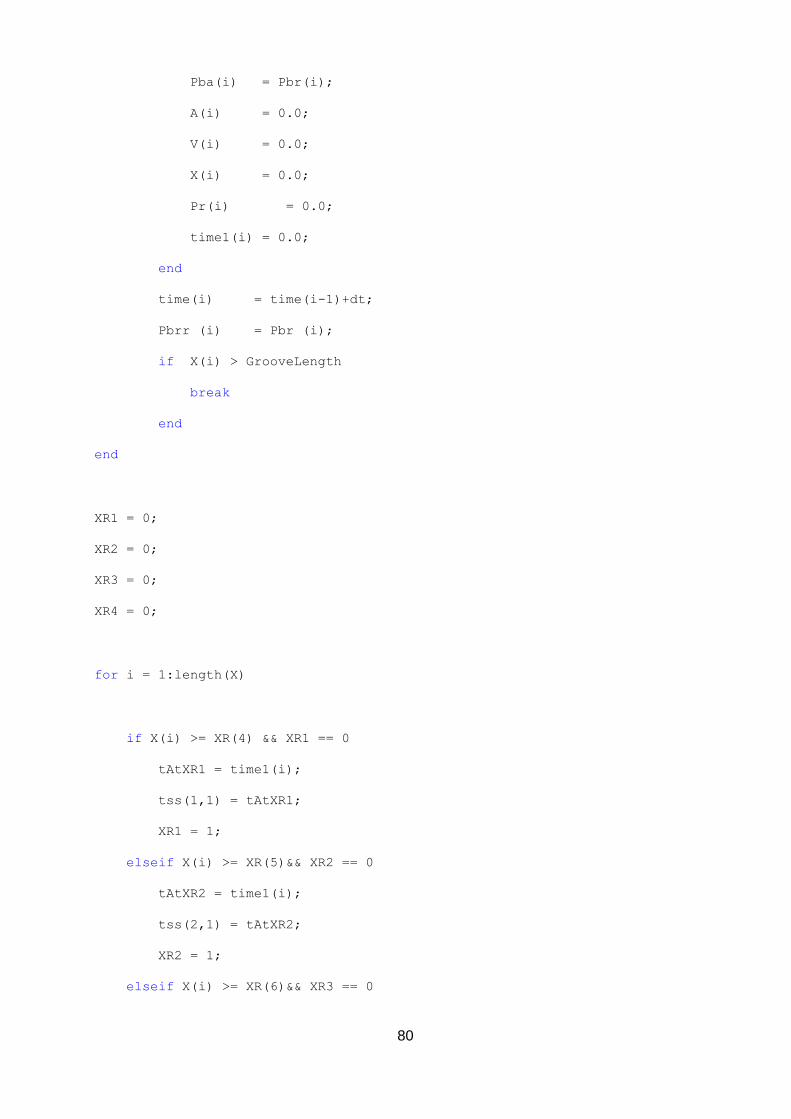
80
Pba(i) = Pbr(i);
A(i) = 0.0;
V(i) = 0.0;
X(i) = 0.0;
Pr(i) = 0.0;
time1(i) = 0.0;
end
time(i) = time(i-1)+dt;
Pbrr (i) = Pbr (i);
if X(i) > GrooveLength
break
end
end
XR1 = 0;
XR2 = 0;
XR3 = 0;
XR4 = 0;
for i = 1:length(X)
if X(i) >= XR(4) && XR1 == 0
tAtXR1 = time1(i);
tss(1,1) = tAtXR1;
XR1 = 1;
elseif X(i) >= XR(5)&& XR2 == 0
tAtXR2 = time1(i);
tss(2,1) = tAtXR2;
XR2 = 1;
elseif X(i) >= XR(6)&& XR3 == 0

81
tAtXR3 = time1(i);
tss(3,1) = tAtXR3;
XR3 = 1;
elseif X(i) >= XR(7)&& XR4 == 0
tAtXR4 = time1(i);
tss(4,1) = tAtXR4;
XR4 = 1;
end
end
display(ts)
display(tss)
V(i)
subplot(2,1,1); plot(XR,PR)
subplot(2,1,2); plot(X,Pr)
function Pr = CalcResistance(x)
% Function to determine resistance pressure as function of x
%
%
global XR;
global PR;
Pr = 0.0;
if x <= XR(2)
Pr = (PR(2)-PR(1))/(XR(2)-XR(1))*x + PR(1); % PR(1) +
Interpolate from X(1) to X(2)
end
if x > XR(2) && x <= XR(3)

82
Pr = (PR(3)-PR(2))/(XR(3)-XR(2))*(x-XR(2)) + PR(2); % PR(2) +
Interpolate from X(2) to X(3)
end
if x > XR(3) && x <= XR(4)
Pr = (PR(4)-PR(3))/(XR(4)-XR(3))*(x-XR(3)) + PR(3); % P((3) +
Interpolate from X(3) to X(4)
end
if x > XR(4) && x <= XR(5)
Pr = (PR(5)-PR(4))/(XR(5)-XR(4))*(x-XR(4)) + PR(4); % P((3) +
Interpolate from X(3) to X(4)
end
if x > XR(5) && x <= XR(6)
Pr = (PR(6)-PR(5))/(XR(6)-XR(5))*(x-XR(5)) + PR(5); % P((3) +
Interpolate from X(3) to X(4)
end
if x > XR(6) && x <= XR(7)
Pr = (PR(7)-PR(6))/(XR(7)-XR(6))*(x-XR(6)) + PR(6); % P((3) +
Interpolate from X(3) to X(4)
end
if x > XR(7) % Beyond X(4)
Pr = PR(7);
end
end

83
PR Function
function Pr = CalcResistance(x)
% Function to determine resistance pressure as function of x
%
%
global XR;
global PR;
if x <= XR(2)
Pr = (PR(2)-PR(1))/(XR(2)-XR(1))*x + PR(1); % PR(1) +
Interpolate from X(1) to X(2)
end
if x > XR(2) && x <= XR(3)
Pr = (PR(3)-PR(2))/(XR(3)-XR(2))*(x-XR(2)) + PR(2); % PR(2) +
Interpolate from X(2) to X(3)
end
if x > XR(3) && x <= XR(4)
Pr = (PR(4)-PR(3))/(XR(4)-XR(3))*(x-XR(3)) + PR(3); % P((3) +
Interpolate from X(3) to X(4)
end
if x > XR(4) && x <= XR(5)
Pr = (PR(5)-PR(4))/(XR(5)-XR(4))*(x-XR(4)) + PR(4); % P((4) +
Interpolate from X(4) to X(5)
end
if x > XR(5) && x <= XR(6)

84
Pr = (PR(6)-PR(5))/(XR(6)-XR(5))*(x-XR(5)) + PR(5); % P((5) +
Interpolate from X(5) to X(6)
end
if x > XR(6) && x <= XR(7)
Pr = (PR(7)-PR(6))/(XR(7)-XR(6))*(x-XR(6)) + PR(6); % P((3) +
Interpolate from X(6) to X(7)
end
if x > XR(7) && x <= XR(8)
Pr = (PR(8)-PR(7))/(XR(8)-XR(7))*(x-XR(7)) + PR(7); % P((3) +
Interpolate from X(7) to X(8)
end
if x > XR(8) % Beyond X(8)
Pr = PR(8);
end
end