THE DEVELOPMENT OF A MARKETING DECISION SUPPORT …

CHAPTER 6

THE DEVELOPMENT OF A MARKETING DECISION

SUPPORT SYSTEM FOR GRAIN PRODUCERS

'There is such a choice of difficulties that I am myself a loss how to

determine. '

- Robert Lowth (1710 - 1787)

6.1 INTRODUCTION

The previous chapters have paved the way for development of a model to

producers in managing investment risk by optimising the use of the various

marketing instruments available to producers. In this study, the model, which is

in this is called a marketing decision support system (MOSS).

The MOSS includes many, although certainly not all, dimensions of a farm

portfolio, concentrating on crop production. The decision alternatives will apply

to producers than to processors or middlemen. At present,

producers can market their crops in three different periods. They can sell their

crops before harvest, using forward contracts, futures contracts and options on

futures contracts; or they can wait and sell in the spot market at or after the

harvest.

The general underlying portfolio theory is a well-known principle of risk

management (Huang & Litzenberger, 1988). decision-maker, or producer,

the composition of the portfolio with the aim of maximising

expected utility. In this study, utility is assumed to refer to profitability. Utility

depends on wealth, and future wealth depends on future returns from

portfolio. Future returns, however, are uncertain. Thus, for the purposes of

166

study, the farm portfolios are assumed to be those of diversified producers of

multiple crops rather than of just single crops. Since and liabilities are an

integral part of all portfolios, allowance is made for the possible effects of debt

and credit on the choice of producers' marketing instruments.

The dynamics of production and price information and their influence on

marketing decisions are mimicked through an updated dynamic (the time

variable is explicitly contained in equations) deterministic control approach. A

deterministic model is one that makes definite predictions for quantities without

any probability distribution. The MOSS employs a of open

loop control problems, each of which is solved while assuming that in

period no additional information is forthcoming. This assumption is however,

revised after each period, when the information is directly observable (Gad &

Ginzberg, 1991). This for example, the producer uses the

information available at planting time to plan the marketing of a certain

percentage of the expected output and then implements decisions that seem

most appropriate to the planting period. Later, at the growing stage, an

additional plan is made using the information available at that point in time, again

marketing a further percentage of the expected output Similar revisions and

occur during the growing stages and at harvest. During these later

periods, the rest of the expected crop can either be sold or stored for later selling

in the spot market Such an approach reflects the fact that marketing

decisions, dependent on evolving information, are made throughout the whole

production-marketing period.

The Province was used as the location where the data necessary to

the MOSS was gathered. The chapter begins with a detailed discussion why

the Free State Province was selected and which statistical regions in the Free

State were finally used collect the data from. The discussion of the analytical

model begins with an explicit statement of the model's underlying assumptions

167

and definitions. This is followed by the development of a decision criterion that

includes both production and price uncertainty. This criterion in turn yields

marketing strategies implied by decision rules. Finally, solution of the model

provides a framework for a discussion of the expected qualitative effects of an

individual farm's characteristics on marketing decisions.

6.2 DATA

6.2.1 Farm unit prototypes

In order to test the ability of farmers to manage risk and market astutely by using

forward markets and derivatives markets, farm prototypes which epitomise the

essential dimensions of commercial grain farms are needed. The details of

prototypes are discussed in terms of marketing period, location, crop

production, production stages and statistical regions.

6.2.1.1 Marketing period

the purpose of this study, period from 1996 to 1999 was chosen because

it represents the new agricultural marketing era in South Africa. The marketing

boards were abolished in 1996 and every producer now carries the responsibility

of marketing his/her own crop. Production patterns (as discussed in Chapter 2)

changed after 1996 and therefore any data prior to 1996 would invalid for this

study_

6.2.1.2 Location

a location, the Free State was chosen. State was leeIeo for two

main reasons. Firstly, is the overall prominence of maize, sunflower seed,

168

Crop varieties and growing techniques vary from one geographical region to

another. The products from the farms of a given province are not homogeneous

in type and quality. Even within a given province, planting and harvesting does

not occur simultaneously on all farms. Because the aim of model developed

in this study is to optimise marketing profits, each farm must be investigated

individually. The crop choice, crop input costs and marketing strategies followed

by the producers were compared with the strategies proposed by model.

6.2.1.4 Production stages

The second step was to allocate months to the production-marketing period for

planting, growing, harvesting and storage. These allocations are presented in

Table 6.1.

175

Table 6.1: Allocating months to the production-marketing period of crops

Maize Planting

Growing

Harvest

Storage

October, November, December

December to April

May, June, July

August to actual selling of crop

Sunflower seed Planting

Growing

Harvest

Storage

November, December, January

January to April

May, June

July to actual selling of crop

Soybeans Planting

Growing

Harvest

Storage

October, November, December

December to April

May, June, July

August to actual selling of crop

Wheat Planting

Growing

Harvest

Storage

May, June

July to October

November, December

December to actual selling of crop

Farm size is the third dimension that needs to be determined for the farm

prototypes. Figure 6.7 depicts the average size of a farming unit for the period

from 1994 to 1996. Due to the fact that more recent data on the average size of

a farming unit in the Free State was not available when the study was done, it is

assumed that the same pattern prevailed for the period from 1996 to 1999.

176

It was not possible to find a farm unit for sunflower production for Category

C in the State. This was due to the that the total production of

sunflower seed in for 1998/99-season was 629 000 tons on

430 000 hectares, resulting in an average yield of 1.46 tons per hectare. On

average, 1 370 hectares of sunflower seed have to planted to qualify for

Category C. The average farm in the State is only 1006 hectares, well

below the required for Category C. By looking at the chosen magisterial

districts (as discussed later in this chapter), it was again not possible to find a

suitable farm unit for Category C.

It is not a prerequisite for the chosen for this investigation to have used the

futures market or derivatives market as a mechanism to manage their investment

risk. Futures markets or derivative markets only provide alternative marketing

strategies to producers. It is the aim of the MOSS to determine optimal

strategy, and a producer might achieve optimum results by ignoring the futures

market.

6.2.1.5 Statistical regions

The fourth entailed the identification of statistical regions, in other words the

regions that have the biggest total income from summer cereals, oil-seeds, and

winter statistically speaking. Figure indicates each statistical region

in the Free State with the percentage gross income from summer cereal. 011

.::>c;~::;u.::> and winter cereals.

179

Districts from Region 28 were used for data on summer cereals and oil seeds,

and Districts from Region 29 for winter crops. Farms from the above

districts in Category A, Category B and Category C are used in the model. Farm

selection, however, was random to ensure that the MOSS could be tested on

producers that had used the derivatives market and also on producers that had

not used the derivatives market. The only requirement was that at least one crop

had been planted and that the total tons produced would be represented in

Categories A, Band C.

6.3 ASSUMPTIONS AND DEFINITIONS

6.3.1 Stage definitions

Assumptions of discrete time were the first step towards making the analysis

viable. The production-marketing time span was divided into a small enough

number of intervals to reduce the dimensions of the model sufficiently to make it

manageable. Yet, time span of the intervals was narrow enough to reflect

the evolution of price and yield information.

and yield uncertainties are strongly related to the dynamics of information.

At planting time, of the current forward contract is assumed to be

known. This assumption ignores the possibility that inflation could change the

value of the forward spot price by the time the contract is exercised. futures

price (for the harvesting period) is also known to the producer. At planting,

however, expected yields are only vague expectations and harvest and post

harvest prices already exist, but the final price expected is only a vague

expectation. By the growing stage and especially as harvest nears, the

uncertainty of yield and price expectations lessens as producers monitor growing

and marketing conditions. At harvest, yields and spot prices during harvest

181

become known and the range of spot prices expected during the storage period

narrows.

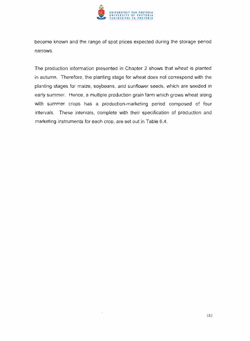
The production information presented in Chapter 2 shows that wheat is planted

in autumn. Therefore, the planting stage for wheat does not correspond with the

planting stages for maize, soybeans, and sunflower , which are in

early summer. Hence, a multiple production grain farm which grows wheat along

with summer crops has a production-marketing period composed of four

intervals. intervals, complete with their specification of production and

marketing instruments for each crop, are out in Table 6.4.

182

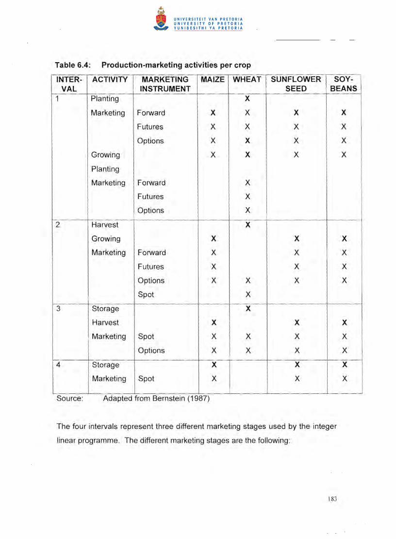
Table 6.4: Production-marketing activities per crop

INTERVAL

ACTIVITY MARKETING INSTRUMENT

MAIZE WHEAT SUNFLOWER SEED

SOYBEANS

1 Planting

Marketing

Growing

Planting

Marketing

Forward

Futures

Options

Forward

Futures

Options

X

X

X

X

X

X

X

X

X

X

X

X

X

X

X

X

X

X

X

X

2 Harvest

Growing

Marketing Forward

Futures

Options

Spot

X

X

X

X

X

X

X

X

X

X

X

X

X

X

X

3 Storage

Harvest

Marketing Spot

Options

X

X

X

X

X

X

X

X

X

X

X

X

4 Storage

Marketing Spot

X

X

X

X

X

X

Source: Adapted from Bernstein (1987)

The four intervals represent three different marketing stages used by the integer

linear programme. The different marketing stages are the following :

183

• Pre-harvest marketing stage. The pre-harvest marketing represents

the time from planting (and any actions taken before planting) to the end of

the growing season. The pre-harvest marketing is reflected by Interval

1 for wheat and by Interval 1 and Interval 2 for summer crops, as depicted

by Table 6.4.

• Harvesting stage. The harvesting stage the time span necessary

for producers to harvest crop. The harvesting stage for wheat is

represented by Interval 2 in Table 6.4 and the harvesting for summer

crops is represented by Interval 3.

• Post-harvesting stage. The post-harvesting stage reflects only the

timespan for crops stored after the harvesting It represents the time

from the end of harvesting to the actual selling of the crops. The post

harvesting stage does not have an upper limit on the time it takes to sell the

crop. producer can store the crop until the harvesting season for the

next year, or even later before selling the crop. post-harvesting stage for

wheat is represented by Interval 3 in Table 6.4 and for summer crops by

interval 4.

6.3.2 Price assumptions

For the purposes of this study, it is assumed that all farms, no matter what their

have the same marketing instruments available to them. farms do

not have any advantages over their smaller counterparts. It is also postulated

that, although production costs are stochastic, they are independent of the prices

of all marketing instruments.

184

Hedgers are temporary substitutes for anticipated actual transactions. This

definition is reflected by the assumption that obligations from short sales in the

futures market are not satisfied through delivery. In addition, once a short

position is taken, the hedge is not lifted by an offsetting futures purchase until the

corresponding harvest occur simultaneously. This implies that, if a

producer into a futures contract during the planting this futures

position will only be offset during harvest time. Speculation is disregarded.

6.3.3 Crop choice

Although the model is based on well-diversified farms, the producer has the

option to choose between the four selected crops, namely white yellow

wheat, sunflower seed and soybeans, as discussed in Chapter 2. The

only prerequisite is that producers must plant at one of the specified crops.

6.3.4 Marketing decisions

The producer can choose between the marketing instruments available in any of

the four production-marketing stages, The producer uses the information

available at Interval 1 to plan the pricing of a percentage of the expected output.

During the early parts of Interval another percentage of the output is

priced. The rest of the expected output is priced during the later parts of Interval

Interval 3 and Interval The same principle applies to producers who plant

only winter crops. They focus on Intervals 1 to and the same principles apply.

185

it that this is not the case in South Africa. indicates the average

tons and the standard deviation thereof for maize, sunflower seeds,

soybeans and wheat obtained in the State.

Table 6.5 Average tons per hectare and standard deviations from

1995/96 to 1998/99

Average yield

1.22 t/Ha 0.24

1.44 t/Ha 0.32

1.29 t/Ha 0.26

2.48 tlHa 0.10

Using the mean as a forecaster of a random variable with a positively skewed

distribution does not result in repeated overestimation. It is therefore not

necessary to adjust yields by making use of Chebyshev's inequalities (Day,

1965).

It is assumed that the decision-maker does not believe that the probability

distributions of crop yields are positively skewed. The MOSS functions on a

continuous basis and the producer can adjust the information as the crop nears

maturity. No producer is committed to sell 100 percent of the crop at planting.

Decision-makers tend to be cautious and want to avoid forward cash and futures

oversales. Therefore, a safety-first strategy is assumed. To obtain this safety

first strategy, only a portion of the expected crop is sold before the critical

growing stages have passed. The rest the expected crop can sold after the

critical growing stages or can be reserved to be sold in the harvest or post

harvest reserves are then available to satisfy forward and futures

commitments if an unanticipated production shortfall occurs. If a producer

decided not to make use of a safety-first strategy the MOSS then also ignored

the safety-first strategy. In order to compare the results obtained by the

187

producer with those of the MOSS, the MOSS must use the same percentage of

crop sold in every stage as the producer.

As the crop year advances and especially as the critical stages of growth for

each product are reached, yield uncertainty diminishes. The probability

distribution of yields becomes more concentrated around the expected value as

weather information is accumulated and the critical growing stages for each crop

are passed. Although the yield uncertainties lessen as the season progresses,

the price risk faced by producers does not diminish over time. This makes it all

the more important to develop an MOSS to producers in managing their

price risk.

6.4 ELEMENTS OF THE MOSS

Decision support systems (DSSs) are an important application of management

information systems (Davis & Olsen, 1985). According to Fang and Puthenpura

(1993), DSSs require use of computers to improve decision-making, and to

allow users data and evaluate alternatives based on models

appropriate to the decisions to be made. Reports on DSSs to optimize

marketing returns for crop farms in South Africa are not available.

MOSS developed in this chapter allows for the possible effects of farm location,

size, and debt on marketing decisions. It also provides for variations in attitude

towards production and price uncertainty.

aim of MOSS is to maximise net return. Net return is the sum of all the

net cash flows generated by all the marketing activities in the different marketing

stages. Net cash flow the difference between cash inflows and cash

outflows associated with crops produced on the farm. Other returns and non-

production are excluded.

188

MOSS aims to determine the optimal combination of marketing strategies

available to producers to maximise net return, given the constraints imposed by

the individual producers. In order to present the model logically, all the cost

components are discussed, followed by the marketing components.

6.4.1 Input cost components

For the purposes of this study, production costs are grouped into three broad

categories:

• Pre-harvest variable cost

Pre-harvest variable include items as

pesticides, labour, transport, fuel and repairs. Interest on production loans

incurred prior to harvesting the crop also have to be included

• Harvest cost per hectare

Harvesting per include costs such as fuel, repairs, labour and

contract work when crop is harvested. These are not affected by

crop yield. reason for treating these costs separately from pre-harvest

costs is the possibility that the crop may not be harvested due to crop failure.

• Harvest per production unit

Harvesting costs per unit of production include cash costs for such as

drying, transport and contract work, which are sensitive to crop yield.

Contract work represents work done by additional labour on a contract basis.

This is normally done in one of two ways. The contract worker can either be paid

per hectare or per ton, so that contract work is distinguished both in harvest cost

189

per hectare and harvest cost per production unit. Farm overhead expenses

should not be included in any of the three input cost categories. For example,

items such as general farm insurance premiums, and returns to operator and

family living expenses should be excluded. The aim of the MOSS is to optimize

crop return by optimizing the net cash flows generated by the various marketing

instruments. Overhead expenses should also be allocated to the rest of the farm

operations. Due to the difficulty in deciding the percentage allocation of

overhead expenses to the crop production process, overhead expenses were

ignored in the development of the MOSS.

Due to the fact that the MOSS aims to maximise net return by choosing an

optimal marketing strategy, the MOSS attempts not to determine the type of crop

to planted, but only the marketing strategy to be used for marketing the crop.

AI! input costs used ignore the influence of the time value of money because the

aim is to optimise the marketing strategy and not to optimise crop choice.

Production in general are assumed to be independent of marketing return.

However, marketing strategies cannot be taken in isolation from input costs.

There is a direct relationship between input cost and the importance of price risk

management. The higher the input cost, the more important effective price risk

management

The requirements for managing cash flows so as to service debt obligations can

also influence marketing decisions. The MOSS incorporates the effects of debt in

the input cost categories by allocating the interest on debt proportionally to the

above categories, and in the discount rate used to determine the present value

of the net cash flow generated by a marketing instrument.

190

6.4.2 Marketing information

For the purposes of this study, producers can decide between pricing their crops

preceding harvest using forward contracts, options on futures contracts and

futures contracts or waiting and selling in the spot market at or after harvest.

The effect of the time value of money is taken into consideration because the

different marketing instruments available lead to different timings of cash flows.

All strategies are discounted back to the harvest date the representative crop.

If a producer has debt obligations, the interest rate associated with debt is used

as the discount rate to calculate the present value of the relevant cash flows. If

the producer has investments, the applicable percentage interest return on these

investments is used as discount rate. If the producer has neither debt nor

investments, the SAFEX interest rate is as the appropriate discount rate.

every marketing instrument, the following information is required:

• selling price (contract price);

• cost (if any);

• handling (if any);

• transport cost (if any);

• brokerage fees (if any);

• premium costs (option contracts);

• delivery date;

• prevailing interest rate (lending rate or investment rate); and

• initial margin costs (futures contracts).

In order to determine the net cash flow of each marketing instrument, the cash

inflows and cash outflows of each marketing instrument must be calculated.

Below, cash outflows are defined and discussed, followed by cash inflows.

191

6.4.2.1 Cash outflows of a marketing strategy

Cash outflows represent all costs that producers incur during the pre-harvest

marketing stage, the harvest marketing stage and the post-harvest marketing

stage. Cash outflows are therefore all costs associated with the planting,

harvesting, storing and marketing of crops. following costs are used in the

equations developed for the model, and they are defined as follows:

.. Storage cost is the cost producers incur if they choose to store their crops to

sell at a later stage.

.. Initial margin is the initial amount required by SAFEX before a producer can

into a contract. Due to the varying of the mark-to-market

prices and the fact that all deposits to SAFEX are paid back after the contract

has been fulfilled, the influence of the maintenance margin is ignored. It is

also assumed that the full amount is always payable.

.. Transaction costs consist of the SAFEX contract cost and commission

charged by the trader.

.. Area differential cost consists of basis cost (the difference between the local

spot price and the futures price of a crop), transport cost from the local

elevator to Randfontein, and handling for loading the crop in and out of

the elevator.

.. Premium cost is the cost per ton to purchase an option on a futures contract.

.. Commission fees represent the total amount to paid when engaging in a

futures or an option contract. It includes commission fees payable to the

trader and all the SAFEX costs (except margin costs) associated with the

action.

Table 6.6 indicates the cost item associated with each marketing instrument.

[92

Table 6.6: Cost items associated with marketing alternatives

x

x

Only spot sales during harvest incur no marketing but the risk associated

with spot sales is much greater. The reason being that producers cannot protect

themselves against any possible downside movement of prices. Normally,

during harvest, the spot price is lower than usual, due to an oversupply of

crop. The opposite can be true as well. Dramatic weather phenomena can push

prices upwards, resulting in higher than average spot sales during harvest.

price movement during harvest cannot be predicted at any time

during the growing season of the crop, it is risky to wait and sell all the crop

during harvest only.

6.4.2.2 Cash inflows of a marketing strategy

Cash inflows represent all cash receipts from the sale of the crop. Cash inflows

therefore represent all receipts of crop during the harvesting and

post-harvesting marketing stage. The effect of the time value of money is taken

into consideration and all cash inflows are discounted back to the harvest date of

the respective crop. The MOSS does not take a short put and a short call option

into consideration. For the purposes of the study, it is assumed that all producers

are not speculative and are only trying to obtain the highest possible price for

their crop. (2000) confirmed that it is more often larger companies who

participate in short puts and short calls. Therefore, the cash inflows from the

193

various marketing instruments are only the price received for the selling and/or

for buying of the crop and not for selling the right to sell crop or to buy the

crop, as is the case with a short put and a short call.

The aim of the MOSS is to the optimal combination of marketing

instruments to optimize the net of producers by taking specific

limitations of the producers into consideration. Equations were developed to

enable the MOSS to choose the optimal combination of marketing instruments.

In order to test the MOSS, the net cash flows of the producers in every marketing

stage are compared to net cash flows of the MOSS. Finally, the net return

generated by the producer's decisions is compared to the net return generated

by the decisions suggested by the MOSS. The first step was to develop

equations to determine the net cash flow of producers for marketing

instrument. equations are adapted to enable the MOSS to

determine the optimal combination of marketing instruments. In Section 6.4.3,

the net cash flow of producers, as a result of their marketing actions, is

determined. Section 6.4.3 is followed by an explanation of integer

programming and the development of the MOSS in this study.

6.4.3 Net cash flow per crop of producers

First, the net cash flow per crop is determined. The net cash flow per crop

represents the difference between cash inflows and the outflows of a

given marketing instrument. The net flow crop is determined by

summarising net cash flows for instrument used To obtain the total

flow of crop sales, the following determinants of net cash flow and

equations to calculate these cash flows are developed:

194

6. 3.1 Net cash flow from spot sales during harvest

The net cash flow from spot sales during harvest is comprised of the following

equations. First, the cash inflow from spot during harvest is determined:

::: P*Q (6.1

Where:

cash inflow from spot

:::P price per ton

:::Q number of tons allocated

Thereafter, the cash outflows of crop sold on the spot market during harvest is

determined:

CFinput ::: {(PHVCN) + (HCPHeN) + (6.2)

Where:

CFlnput :::

y :::

PHVC:::

HCPHe:::

HCPU:::

input cost

yield per hectare (ton)

pre-harvest variable cost per hectare

harvest cost per hectare

harvest cost per ton

combination of Equations 6.1 and 6.2 results in the net cash flow from spot

sales during harvest for all the crops covered by the MOSS.

:::NCFspot

Where:

195

::NCFspot net cash flow from spot during harvest

Equations 6.1, 6.2 and 6.3 can only used to determine the cash flows from

spot during harvest. The receipts from the spot sales during harvest are

received immediately and it is therefore not necessary to take the of the

time value of money into consideration. If a producer decides to delay the selling

and delivery of the crop, the of time value of money must be taken into

consideration and not form part of the harvesting marketing

6. 3.2 Net flow from storage

The equations developed to determine the net cash flow from storage (all the

that occur in the post-harvesting marketing stage) differ from the equations

developed in Section 6.4.3.1. The reason for this is the of the time value

of money. The discount rate used in determining the present value is influenced

by the producer's debt position. If the producer uses a production loan from a

co-operative, and/or makes use of a bank overdraft facility in the crop production

process, the highest debt interest rate is used. If the producer not use any

debt financing and has investments, the percentage interest return on these

investments is used in the discounting process. If the producer does not use any

debt financing, nor has any investments, the interest on the day the

contract is entered into, is used as a fixed rate throughout the marketing season.

To determine the net income from storage, the equations below therefore apply.

First, the cash outflows associated with the storage decision is calculated:

Where:

C F store/out cash outflows resulting from the storage decision ::

196

PV present value

S storage cost per ton per day

T length of storage (in days)

The net flow from storage decision is determined by:

Netstore == PV(P*Q) - CF,nput - CFstore,out

Where:

Nets\ore ::: net cash flow from store alternative

CF,nput == input costs (Equation 6.2)

C F store/out ::: cash outflows resulting from storage decision

The cash inflows and cash outflows are discounted to the value at

harvest time. This enables a comparison between the different marketing

strategies. The storage alternative only forms part of the post-harvesting

marketing and the net return generated by storage is therefore only

reflected in the post-harvest marketing stage.

6.4. 3 Net cash flow from forward contracts

net cash flow for forward contracts (all the forward sales that occur in the

pre-harvest marketing stage) can consist of two possible equations. If the

delivery is made during harvest, the following equation is applicable:

net cash flow from forward sales delivered during harvest

cash inflow from spot sales (Equation 6.1)

J97

CFlnput ::::: input cost (Equation 6.2)

Although the producer can already enter into the forward contract during the pre

marketing stage, the payment is only received on delivery. Because the

payment is received during harvest, the effect of the time value of money can be

ignored and the flow represents a spot sale during harvest.

If delivery on the forward contract is delayed to a later stage, the following

equation that takes the storage cost and time value of money into account is

used:

NCF fw = PV(P*Q) - CFlnput

Where:

CFstore/out cash outflows resulting from the storage decision

(Equation 6.4)

6.4.3.4 Net flow from futures contracts

In the case of futures contracts, the net flow can be influenced by the

following two sets of scenarios:

• whether the producer can maintain the margin calls or not; and

• whether the producer closes out his/her futures position, or delivers on the

futures position.

Futures contracts are discounted to harvest time to enable comparison between

the various instruments. The length of time used in the discounting process is

the time from harvest to the expiry date of the futures contract.

198

If the producer maintain the margin calls and decided to deliver on the futures

position, the net cash flow is determined by the equations below.

First, the cash inflow resulting from a futures position is determined:

Where:

inflow from futures sales

FP :::: futures price per ton

:::: interest per day

Mar :::: initial margin

The cash outflow resulting from futures position is determined:

CFfUt!out :::: (TC*n)

Where:

CFfUt!out= cash outflows resulting from futures contracts

:::TC total transaction cost per contract

:::;n number of contracts

net cash flow from delivery on futures is determined by:

CFlnput (6.10)

Where:

NCFfut :::: cash flow from contract sales

A :::: area differential cost

199

If the producer cannot maintain margin calls and has decided to deliver on

the futures position, following equations apply:

cash inflow from futures position is determined:

CFfUtfin :::: PV(FP*Q) (6.

Where:

CFfUtfin =. cash inflow from futures sales

net cash flows resulting from the futures position is thereafter determined.

Where:

NCFfUtfidl =. net cash flow resulting from futures contracts

to the fact that the producer has to borrow the initial margin, the interest

by the margin account (i*Mar) is seen as a cost. If the producer could

maintain the margin interest generated by the margin account is seen

as a cash inflow and it is assumed that the producer could have invested the

initial margin amount to earn an income.

If the producer can maintain the margin calls and decides to close out the

short futures position with a long position, the net cash flow is determined

by following equations:

(6.13)

Where:

200

NCFsfutc!= net cash inflow of short futures position closed out

FPs = short futures price per ton

FPI = long futures price per ton

And if the producer decides to close out the long futures position with a short

futures contract, the net cash flow resulting from this action is determined by

Equation 6.14:

NCFlfutc, = PV(FPI - FPs)*Q - (TC*n) (6 .14) I

Where:

NCFlfutci = net cash inflow of long futures position closed out

On the other hand if the producer cannot maintain the margin calls and

decides to close out the short futures position with a long futures position , the

net cash flow is determined by the following equation:

NCFsfut = PV(FPs - FPI)*Q - (TC*n) - (i*Mar) (6 .15) I

Where:

NCFsfut = net cash inflow of short futures position

And if the producer cannot maintain the margin calls and decides to close out

the long futures position with a short futures contract, the net cash flow resulting

from this action is determined by Equation 6.16:

NCFlfut = PV(FPI - FPs)*Q - (TC*n) - (i*Mar) (6.16) I

Where :

NCFlfut = net cash inflow of long futures position

201

It is assumed that in the pre-harvesting marketing stage the producer will deliver

on futures contract. Equation 6.10 is therefore used in determining the

cash flow of futures during the pre-harvest marketing stage.

6.4.3.5 Net cash flow from options on futures contracts

When producers use option contracts, a choice can be made between put

options and call options. Producers normally enter into a put option contract if

they expect prices to decline. Producers normally into a call option

contract to protect themselves against a price jf they forward contracts

to sell a percentage of their crop. If producers choose a call option contract, they

have the right to buy the commodity at a specific price. Producers can also use

call option contracts to lengthen the marketing time of their crops. Producers sell

their crop during harvest and purchase, for instance, a March call option contract

if they expect prices to If the price of the grain producers can, for

example, their option before the expiry date of the call option, buy the

commodity at the predetermined price and sell it immediately in the spot market

for a higher price. To determine the net cash flow from options on futures

contracts, the following scenarios apply:

• put option contracts exercised and delivered;

• put option contracts exercised and futures position closed out;

• put option contracts expired worthless;

• call option contracts exercised and delivery received;

• call option contracts exercised and futures position closed out; and

• call option contracts that expired worthless.

The following equations were developed to determine the cash flow for

various scenarios of options on futures contracts.

202

If a producer decides to exercise a put option contract and to deliver on the

contract, the following equation is to determine the net cash flow:

NCFputJex = PV{(P*Q) - (A*Q)} (TC*n) - CFinput (6.1

Where:

NCFputJex= net cash flow from put option contracts exercised and

delivered upon

Prem = premium per ton

If a producer decides to exercise a put option contract, to close out the futures

position and the sell the crop on spot market, the following equation is used

in determining the net cash flow:

NCFputJcI = PV{(P*Q) + NCFsfut} (TC*n) CFinput

Where:

NCFputic, ::: net cash flow from put option contracts exercised

and closed out

NCFsfut ::: net cash inflow of short futures position

If the put option contract expired worthless, the net cash flow is determined as

follows:

:::NCFputinex -{(TC*n) + (Prem*Q)} (6.

Where:

::::NCFputinex Net cash flow from put option contracts not

exercised

203

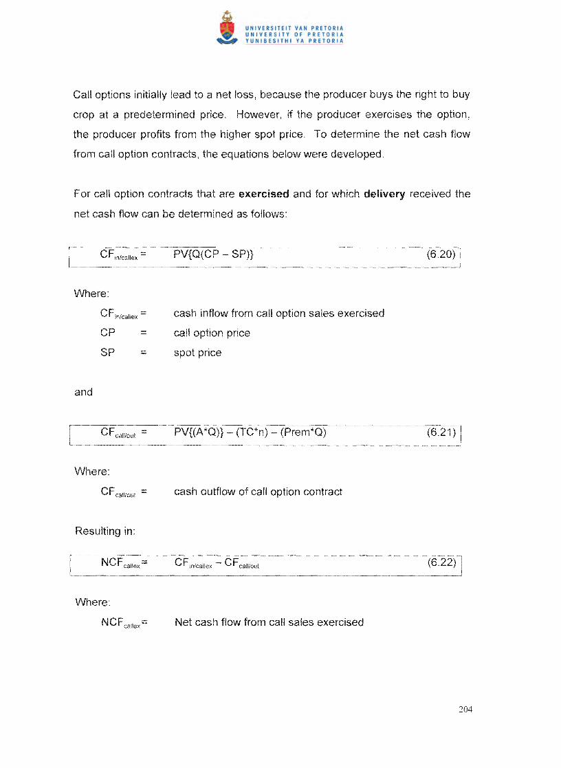
Call options initially lead to a loss, producer buys the right to buy

crop at a predetermined However, if the producer the option,

the producer profits from the higher spot To determine the net cash flow

from call option contracts, the equations below were developed.

For call option contracts that are exercised and for which delivery received the

net cash flow can determined as follows:

:::: PV{Q(CP - SP)}

Where:

:::: inflow from call option sales exercised

CP :::: call option price

:::: spot price

and

C F call/out ::: PV{(A *Q)} - (TC*n) (Prem*Q) (6.21 )

Where:

CFcall/out :::: cash outflow of call option contract

Resulting in'

CFin/callex - CFcall/out

Where:

N C F callex::: Net cash flow from call sales exercised

204

If a call option contract is exercised and the position is closed out, the net cash

flow is determined by:

NCFcaliCI ::: PV{(Q* NCFlfut )} - (TC*n) (6.23)

Where:

NCFlfut :::; net cash inflow of long position

NCFcallcl :::; net cash flow from call option sales exercised and

closed out

call option contracts that expired worthless,

developed:

the following equation is

:::: + (Prem*Q)} (6

Where:

NCFcallnex :::: net cash flow of call option

worthless

contract that expired

In the pre-harvest marketing it is assumed that all option contracts are

exercised and delivered. The net cash flow from put option contracts is therefore

determined by Equation 17.

205

Finally, the net return generated by the producer is determined as follows:

+ NCFfwh + NCFfw + NCFfut + (6Net return :: NCFspot +

NCFsfutel+ NCFlfwel + NCFsfut + NCFlfut + +

NCFputiCI + NCFputinex + NCFcallex + NCFcalicl + NCFcallnex

Where:

Net reurn :: net return of crop

Appendix A serves as an example to illustrate how the various flows

and returns is calculated and shows the marketing making process of

producers.

6.5 SOLUTION METHOD

Optimisation problems can be divided into unconstrained and constrained (any

restriction the decision variables must satisfy) variables, and the latter into

problems with equality constraints (where x :: 0) and problems with inequality

constraints (where normally x ~ 0). Inequality constraint problems also

x > O. Thus there are three broad categories in which problems can be

classified, and the corresponding solution methods were determined in two

different eras.

Unconstrained optimisation problems were first solved with the methods of

calculus, developed in the seventeenth century by Newton (1642-1727)

and Gottfried Wilhelm Leibniz (1646-1716). The solution to optimisation

problems constrained by equalities was found a century later by Joseph-Louis

Lagrange (1736-181 For inequality-constrained problems, the solution

206

procedures were not found until the 1940's, by John von Neumann and George

Dantzig (Fang & Puthenpura, 1993). Optimisation with inequality constraints

differs in one fundamental respect from the earlier problems: is no closed,

analytic expression describes the solution. Therefore, it is necessary to

know the optimal basis, or the list of the variables that appear in the optimal

solution.

Linear programming is a mathematical that is often helpful In solving

decisions requiring a choice between a number of

theoretical concepts underlying the methods of linear programming been

known for many However, it was during World War II and immediately

thereafter that the application of linear programming to planning problems was

Since then techniques have been applied increasingly to

management decisions in various industries, including in agriculture. Linear

programming is concerned with problems in which a linear objective function in

terms of decision variables is to optimised (Le., either minimised or

maximised) while a set of linear equations, inequalities, and signs (positive or

negative values) are imposed on the decision variables as requirements.

Optimisation problems for linear programming are made up of three basic

ingredients:

• an objective function which has to minimised or maximised;

• a set of unknowns or variables which affect the value of the objective

function; and

• a set of constraints that allow the unknowns to take on certain values but

exclude others.

207

If the objective function is for example:

and x2 so as to: x1

Maximise Z ::: 5x1 + 2X2

Where:

x1 ::: variable 1

x2 ::: variable 2

The following step entails the identification of all the different constraints on the

problem. Assume the constraints are the following:

model formulation the above maximisation problem is presented

graphically in Figure 6.11 In order to graph the two constraint inequalities (~), it

is necessary to as an equality By finding two points common to

each equation, the lines can be determined and plotted on the graph. A method

of plotting a line is to let one variable in an equation equal zero. For example, in

x1 + x2 ~ 8 let x1 ::: 0, then ::: 8 and let ::: 0, then x1 ::: 8. paints are

connected with a line in Figure 6.11 (a). For the constraint, 4Xi + x2 ~ 12 x1

then ::: 12 and let x2 == 0, then 4x1 ::: 12 and X1 ::: points (Xi == 0, :::

12 and X1 ::: 3, ::: 0) are then plotted on each axis and connected with a line in

Figure 6.11 (b).

208

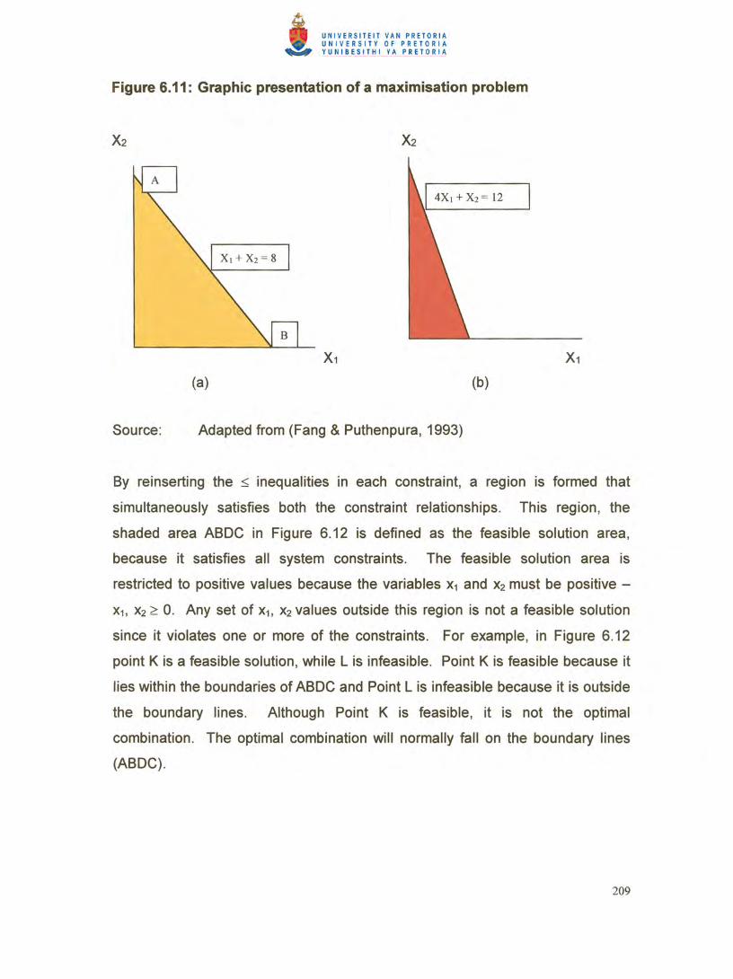
Figure 6.12: Feasible and infeasible solutions

X1

Adapted from (Fang and Puthenpura, 1993)

c

Source:

The final step is to evaluate the objective function (5X1 + 2X2) at pOints A , B, D

and C to determine which one(s) is optimal. This is accomplished in Table 6.7 .

Table 6.7: Candidate solutions

Extreme points Co-ordinates

(Xh X2)

Objective function value

(5X1 + 2X2)

A

B

C

D

0,8

(4/3),(20/3)

0,0

3,0

16

20

° 15

Point B occurs at the intersection of (X1 + X2 = 8) and (4X1 + X2 = 12), or {X1 = (4/3)

and X2 = (20/3)}. Since point B gives the maximum value (20) for the objective, it

is the optimal combination.

210

The mathematical specification of an integer linear programming problem is the

same as for a linear programming problem, with one exception. In addition to

requiring the levels of all variables in a solution to be greater than or equal to

zero, some or all variables can be required to take only zero or values, as

opposed to fractional values. Integer linear programmes have the advantage of

more valuable for the purposes of study as compared to ordinary

linear programming, in the sense that integer values is now also taken into

consideration. The most widely used approach in integer linear

programming requires a series of linear programmes to manage the search for

integer solutions and to prove optimality.

Integer programming has proved valuable for modelling many and diverse types

of problems in planning, routing, assignment and design. Industries that use

integer programming include transport, energy, telecommunications,

manufacturing and agriculture (Ferris, 1998).

Mixed integer programming requires that only some of the variables need to

have integer values, whereas pure integer programming requires all variables to

be MOSS developed in this chapter is based on mixed integer

linear programming. The reason for this lies in the fact that futures contracts

and options on futures contracts can only be for values of 100 tons and the

multiples thereof.

6.5.1 Net cash flow used by MOSS

mathematical model developed in this chapter consists of marketing

activities as the basic building blocks. With the aid an integer linear

programme built on a spreadsheet, various combinations of these actions can

211

evaluated in terms of their impact on cash inflows and cash outflows, as well as

other constraints that might be placed on their combination, and the objectives of

the farm concerned.

The MOSS uses constraint optimisation to determine the optimal combination of

marketing instruments that result in the highest net return. The net return is

defined as the sum of the net cash flows from all the various marketing

instruments available. Before integer linear programming can be used to solve

an optimisation problem, certain constraints must be defined. The constraints

used in this MOSS were the minimum and maximum number of tons that a

producer was willing to allocate to a marketing instrument and the cash

flow position of the producer. If the producer experienced flow problems,

futures contract can be excluded from determining the optimal combination.

In order to determine the optimal cornbination of marketing instruments, net

cash flow per ton of each marketing instrument has to be determined.

Furthermore, the various equations developed in Section 1 to Section

6.4.3.5 were adjusted for application to the MOSS to determine the net cash flow

per ton. The MOSS used therefore the same equations with the only change

that the net cash flow is determined per ton.

Appendix A serves as an example to illustrate how the various net cash flows

and returns by the MOSS is calculated in determining the optimal combination of

marketing actions.

6.6 CONCLUSION

Producers must repeatedly make decisions about what commodities to produce,

by what production method, in what quantities, and how to sell them. Decisions

212

are made subject to the prevailing physical and financial constraints of the farm

and often in the face of considerable uncertainty about the planning period

ahead. Uncertainty may in the expected yields, costs and for the

individual farm enterprises, in fixed requirements and in the total supplies

of the fixed assets available.

Traditionally, producers have relied on experience, intuition and comparisons

with their neighbours to make their financial decisions. However. formal

techniques of budgeting and comparative analysis have now developed by

farm management specialists, and these can be useful aids for making decisions

in complex situations or for analysing selected decisions when all the other

farm decisions are taken as given. More advances in computers and in

mathematical programming software mean that satisfactory procedures have

now been developed for total farm planning in more complex situations.

Total farm planning can assist producers to adapt efficiently to a changing

economic and technological environment. Mathematical programming in

agriculture had its origins in attempts to model the economics of agricultural

production, including spatial dimension. mathematical programming

format is particularly suitable for agriculture. Producers, agronomists, and other

agricultural specialists share a common way of thinking about agricultural inputs

and outputs in terms of the annual crop cycle, and about input-output coefficients

per Yields are conceived in tons per hectare, fertiliser applications in

kilograms per hectare and so on.

By means of integer linear programming, attempts were made develop first

MOSS suitable for South African producers. The aim of the MOSS developed in

this chapter is to determine optimal combination of marketing instruments to

optimize crop net return. First, the net cash flows of producers by using various

marketing instruments were determined. Thereafter, the return per ton for

2J3

marketing instrument was determined. Using integer linear programming

the optimal combination of marketing was determined. The next

chapter indicates how the MOSS was tested to prove its viability.

214

CHAPTER 7

APPLICATION OF THE MARKETING DECISION

SUPPORT SYSTEM

If a man look sharply and attentively, he shall see Fortune; for though she

is blind, she is not invisible

- Francis Bacon (1561 - 1626)

7.1 INTRODUCTION

The previous chapters the changing agricultural environment in South

Africa, different types of risk that producers are with and pricing

instruments available to producers who wish to manage price risk. Chapter 6

focused on the development of a Marketing Decision Support System (MOSS)

for grain producers in South Africa. This chapter discusses the application of the

MOSS and its empirically testing. MOSS allows for the possible of

farm location, farm debt on marketing decisions. It also provides for

variations in attitudes towards production and price uncertainty.

In economic terms, a well-managed farm is one that consistently makes larger

net profits than similarly structured neighbouring farms. random

localized such as weather patterns mask differences or similarities

in management, it is important to observe differences in profits that persist over

time. A crop producer can enhance the farm's revenue by better use and

application of technology, improved cost management, improved yields and

higher prices due to better marketing strategies. This chapter focuses on the

application of MOSS in primary function of managing price risk. Producers

have many alternatives for managing agricultural risk. They can diversify the

2]5

farm business or the financial structure of the business. in addition, producers

have access to various instruments, such as insurance and hedging, that can

help reduce their farm's level of risk. Indeed, most producers combine many

different strategies and instruments and formulate strategies to hedge against

the risk possible losses.

Because producers vary in their attitudes towards risk, risk management cannot

be viewed using a 'one fits all' approach. Different producers have to

confront different situations, and their regarding risk and their

return trade-offs an important effect on decision-making in each given

situation. This chapter investigates the application and usefulness of the MOSS

as developed in this study for grain producers in South Africa.

7.2 AREAS OF RISK EXPOSURE

The preceding chapters various price risk management

instruments available to producers in South Africa. It is essential that producers

understand how to use various pricing instruments to manage price risk and

how to select the most appropriate pricing instrument to accomplish their

objectives of sustainable, profitable farming. Some instruments manage only

one of the primary market risks, while others may manage several types risk.

Knowing how use the various instruments involves understanding the

mechanics of such aspects as opening a trading account with placing

orders with a broker and meeting margin requirements. It also includes

understanding obligations and responsibilities for delivery, and conditions under

which contracts can cancelled or modified.

216

Selecting the most appropriate pricing instrument for a farm's financial and

marketing situation is complex. The most appropriate pricing instrument is

mainly determined by the following aspects:

• the producer's risk management and expectations regarding

future price movements;

• current price relationships and expectations regarding changes in those

relationships;

• the producer's attitude towards risk.

More than one pricing instrument may be available to accomplish a producer's

objective. An important aspect of the decision process is to assess the risk

with each pricing instrument. The following two questions provide

guidelines in choosing the right instrument:

(i) What does the producer want to accomplish?

(ii) What is the best way to reach the financial objectives of the producer?

The main areas of farm risk were identified and examined in Chapter 3 as yield

risk, price risk, institutional risk, personal risk, exchange rate risk and financial

risk. risks affect a producer's net income and should also be considered

in the selection and implementation of pricing instruments. risks can be

summarised as follows:

• Cash flow risk is typically associated with trading in futures. It is the risk that

the producer is unable to maintain a margin account to a shortfall cash

on hand. a margin account is established and a futures position is

taken, adverse price movements may require additional deposits in the

margin account. Rising from a short futures position, for example,

would result margin calls. Conversely, declining prices would in

money flowing into the margin account a short futures position to the

decline in the of the grain owned.

217

• Business or counter-party risk is the risk associated that the grain buyer

will not be able to fulfil part or all of the contract agreement. The risk is

especially important for producers who have forfeited their title to the grain,

but have not yet received payment. Business failure is likely to result in the

cancellation of forward contracts, leaving the producer in an open position on

grain that was priced earlier.

• Volatility risk (as discussed in Chapter 5) is associated with the options

market. The risk lies in the fact that option premiums do not change one-for

one with cash or futures prices, so that the net prices on such contracts do

not move one-for-one with the change in price level. The extent of the risk

varies with market volatility, the closeness of the options strike price to the

underlying futures price, the length of time until the contract expires and

whether the producer intends to hold the option position until maturity or to

exit early.

• Yield risk arises when the producer sells a crop prior to harvest. The primary

concern is that production volumes may fall short of expectation. The extent

of yield risk varies with the type of pricing instrument used. When a producer

enters into a short futures position or a forward contract, the producer is liable

to deliver on the size of the contract When yield is lower than expected, the

producer can offset a short futures position by entering into a long futures

position. This might occur at a higher price than the original short futures

position. Producers can protect themselves against lower than expected

production volumes in forward contracts by a force majeure. A force majeure

gives producers the right to deliver volumes smaller than originally signed for.

The seller of the forward contract normally grants this protection at a

discounted price compared to a forward contract without a force majeure.

2]8

Although the following risks are not discussed length in Chapter 3, they also

affect price risk management alternatives:

.. Grain quality risk is the risk that grain is graded lower due to disease or

extreme weather conditions, and is subject to price discounts. This risk is

associated with all pricing instruments.

.. Tax risk includes the risk that losses associated with positions in the futures

and options markets will be capital versus ordinary business

.. Control risk is the risk associated with the number of decisions required to

implement a pricing instrument fully. Some instruments require only one

decision, a cash grain sale, for example. Other instruments, such as futures

and options, require an initial decision and one or more subsequent

decision(s). When a series of decisions is required, there is a risk of adverse

market action that will reduce the profit before subsequent decisions are

made.

Farming, like any business enterprise, involves taking risks to obtain a higher

income than might be obtained otherwise. Some producers appear to virtually

disregard risk. But for most, the risk they can accept is limited. Thus, price risk

management is not a matter of minimiSing price risk, but of determining how

much risk to take, given a producer's alternatives and preference trade-offs.

the producer's choice between different pricing instruments is also

influenced by the sensitivity of the pricing instruments towards the areas of risk

exposure, as indicated by Table 1.

219

Table 7.1: Areas of risk exposure

(I) ~ In> 0 ~ InPricing alternative (I) ;;:: (I) 0 ~ Risk rating

:;:; c '(I) ~ - "C (J In C\J In >< C C\J .~ C\J 0 = C\J 0 Q) = a.. u > m I U > 0

Selling out of inventory or establishing pre-harvest price levels

Cash sales x x x Moderate to high

Forward contracts x x x Low to high

Short futures x x x x Low to high

Buy put options x x x x x Low

Price grain & buy call option x x x x x x x Low

Minimum price contracts x x x x x x Low

Retaining ownership

Storage x x Moderate to high

Sell grain , buy futures x x x x Moderate to high

Sell grain , buy call options x x x x Low

Minimum price contracts x x x x Low

Delayed pricing contracts x x x Moderate to high

Source: Adapted from Ferris (1998)

220

It is from Table 1 that some grain pricing instruments are exposed to

higher risk than others. instruments are designed to manage

aspects of risk. Instruments can be used in combination to risk

management capabilities. The usefulness of the MOSS is compared with the

areas of risk exposure of instrument. Some producers in the study

indicated that they are not interested in certain instruments, due to the level of

risk exposure of that instrument, and they were consequently excluded from the

analysis. Table 1 serves as a guideline for producers in their decision-making

process and instruments of the MOSS are examined in of

risk exposure Table 7.16).

THE SURVEY

A questionnaire was developed to collect data from crop producers in the

State Province. The data was collected in the form of a postal survey, followed

by telephonic interviews and personal interviews. Crop producers in Statistical

Regions 28 and in Free State Province were randomly selected from

address lists provided by local co-operatives and agri-businesses. From the

postal survey, a response rate of 28% was obtained postal survey was

augmented by telephonic interviews and personal visits. The for the

analysis were obtained from 14 producers in above statistical regions. This

resulted in a final response rate of 78%. None of the questionnaires were

unusable due to incomplete information. Information regarding marketing

strategies was collected from producers during the 1998/99-marketing

season for summer crops and the 1999/2000-marketing season for wheat.

reason why the MOSS was not tested for longer periods was that during its initial

was used as a guaranteed forward pricing market with high levels

of physical Options on futures contracts only started trading in March

221

1998 and therefore the marketing seasons before the 1998/99 marketing season

were unusable.

From the responses to the questionnaire, it seems that respondents spend an

average of 3.2 hours per week reviewing marketing information. Weekly

agricultural magazines were rated the most important sources of price

information, followed by subscription-based information providers and SAFEX.

When producers were asked to identify their needs for additional information and

services to manage their grain marketing better, the most commonly requested

service was information on price and production trends in international markets.

Producers generally rated their skills in marketing management lower, than their

production and financial management skills.

7 .4 EVALUATION PROCUOURE FOR THE MOSS

The MOSS is based on the principles of integer linear programming. Firstly, the

information pertaining to the producer was entered into the model. Every time a

producer made a decision, the result was compared to the net effect suggested

by the MOSS. From there on, the decisions suggested by the linear programme

were taken into consideration in future decisions. For instance, when the model

suggested that the producer should engage in a short futures position, the

futures position was reflected in the next set of decisions. All option contracts

suggested by the model were at-the-money, due to the difficulty in deciding how

much an option must be in- or out-of-the-money.

Secondly, one month prior to harvest, the MOSS was run again to sell a total of

about 80% of the producer's crop. If the producer had already sold more than

80% of the crop one month prior to harvest, this action of the MOSS was

ignored. The primary reason for this action was that the spot price during

222

harvest normally tends to be lower than prior to the harvest. By selling about

80% of the crop, a producer protects himself/herself from price risk, and the

possibility of yield risk is much smaller than earlier in the season .

It is important to take note that in the case of sunflower seed, the first contracts

were traded on 1 February 1999. Any decisions made by producers before that

date could not be compared with other marketing alternatives available to

producers. Soybean prices and strategies available to producers were limited to

local prices. No international price risk instrument was taken into consideration ,

due to the fact that South Africa is a net importer of soybeans and therefore the

soybean prices always reflect the import parity price of international soybeans.

All the pricing tools available to producers for maize and wheat were taken into

consideration by the MDSS (except in cases where producers specifically

excluded certain instruments).

7.5 ANTICIPATED EFFECTS AND CASES INVESTIGATED

The analytical model used in this study allows for the possible effects of farm

location , size and debt on marketing decisions. The model also provides for

variations in attitudes towards production and price uncertainty. The complexity

of the solution presented by the model resulting from the interrelatedness of

these factors, however, is not conducive to simple, mathematically derivable

comparative statistics. The purpose of this investigation , as stated previously,

was therefore to investigate the sensitivity of the model to the instruments used

in order to obtain the highest possible profit generated from the crops planted .

223

7.5.1 Investigation results

The marketing strategies corresponding to the 14 cases investigated are set out

in Tables 7.2 to 7.15. For each case, information on the actual quantities (in

tons) of each crop sold using each marketing alternative during the 1998/99

marketing season for summer crops and the 1999/2000 marketing season for

wheat are also given. The net returns obtained by the producer and the MOSS

are calculated using Equations 6.1 to Equation 6.25.

The sales in tons reported in these tables were not conducive to comparisons in

terms of farm size or location . Therefore , the information was converted to the

percentage of annual output marketed by the producer using each alternative.

The marketing actions of the producers and the MOSS were divided into three

different marketing stages:

• pre-harvest stage (actions taken before planting, during the growing season

until harvest time);

• harvest stage (actions taken during the harvest season); and

• post-harvest stage (actions pertaining to the current marketing season after

the harvest period, with no time limitation on the post-harvest stage).

The dates used in the testing of the MOSS are the same dates as those used by

the individual producer when a marketing decision was made. Producers did not

make marketing decisions on the same date, however, which means that the

dates used in the testing of the model also vary for each individual producer.

7.5.1.1 White maize producers

The investigation took into account the different categories discussed in Section

6.2.1.4, Category A with a total crop production of less than 1 00 tons, Category

224

B with a total crop production between 1 000 tons and 1 999 tons, and Category

C with a total crop production of 2 000 tons and more.

• Producer A 1

The farm unit of Producer A 1 is situated in Statistical Region 28 of the Free State

Province. Producer A 1 planted 133 hectares of white maize with a realised yield

of 4,7 tons per hectare (classified in Category A) . On 25 February 1999 he

entered into a forward contract to deliver 200 tons of maize, which represents

32% of the total white maize crop, to a local elevator owner at a price of R850

per ton. During the harvest period, he sold the remainder of his crop on the spot

market, at a price of R700/ton. Table 7.2 displays the results of Producer A 1 's

actions as well as the results of the actions suggested by the MOSS.

Table 7.2 Comparative net returns - Producer A1

Actions Pre-harvest stage

25/2/99

Producer A1 MOSS

Pricing instrument and % sold

Net cash flow

Forward (32%)

R93715

Forward (32%)

R93715

14/05/99


Net cash flow

Harvest stage

14/06/99

0% Short futures (48%)

R99387


Net cash flow

Spot market (68%)

R105768

Long futures (48%)

Spot market (68%)

R115400

Net return

% improvement

R199483 R209116

4.85%

225

The MOSS suggested the following marketing instruments during the 1998/99

marketing season:

Pre-harvesting stage

In the pre-haNesting stage the MOSS suggested that 32% of the crop should be

sold using forward contracts. One month prior to haNest, the MOSS was run

again to sell a total of 80% of the expected crop of Producer A 1. The

instruments suggested by the MOSS were to:

• sell 200 tons of maize on a forward contract on 25 February 1999; and

• engage in a short futures position (three contracts) at a price of R884/ton on

14 May 1999.

Harvest stage

The MOSS suggested that the producer should:

• deliver on the forward contract; and

• close out the short futures position with long futures contracts at a price of

R863/ton and sell the rest of the crop on the spot market.

Producer A 1 sold all the crop during harvest and did not participate in any post

haNesting strategies. The actions suggested by the MOSS generated an

improvement of 4.85% on the net return of Producer A 1. Producer A 1 received

exceptionally good prices from his forward contract compared to the futures

contracts at that stage. The prevailing futures price during the same time was

only R723 per ton , resulting in a very strong basis. The only negative aspect of

the producer's strategy was that the producer had locked himself out of any

possible future price increase.

226

• Producer A2

The farm unit of Producer A2 is in Statistical Region 28 of the Free State

province. Producer A2 planted 400 hectares of white maize with a realised yield

of 4 tons per hectare. The total production volume of Produce A2 is 1 600 tons

and he is therefore classified in Category B. The producer followed the following

marketing strategies:

• On 15 March 1999 he entered into a forward contract to deliver 800 tons of

maize to a local elevator owner at a price of R550 per ton .

• He sold the remainder of his crop (800 tons) on the spot market during the

harvest period and received an average price of R550 per ton .

The producer indicated that he did not want to sell any maize on the futures

market due to cash flow problems. No further constraints were indicated on any

other pricing alternative. Table 7.3 combines the results of Producer A2 to those

of the MOSS.

227

Table 7.3: Comparative net returns - Producer A2

Actions Producer A2 MOSS

Pre-harvest stage

15/03/99


Net cash flow

Forward (50%)

R129120

R880 put (50%)

R336236

21/05/99


Net cash flow

Harvest stage

20/06/99


Net cash flow

0%

Spot market (50%)

R129 120

R900 put (30%)

R249402

Exercise puts (80%)

Spot market (20%)

R511 223

Net return

% improvement

R258240 R511223

97.96%

The MDSS suggested the following actions during the 1998/99 marketing

season, which generated a 97.96% increase in net returns :

Pre-harvest stage

• Eight put option contracts with a strike price of R880/ton should be purchased

on 15 March 1999.

• Six put option contracts with a strike price of R900/ton should be purchased

on 21 May 1999, one month prior to harvest.

Harvest stage

• On 21 June 1999 all the put option contracts were to be exercised and 200

tons of maize were to be sold on the spot market.

228

• Producer A3

The farm unit of Producer A3 was in Statistical Region 28 of the Free State

Province. Producer A3 planted 850 hectares of white maize with a realised yield

of 4 .59 tons per hectare (classified in Category C) . The producer followed the

following marketing strategies:

• On 12 November 1998, he entered into a forward contract to deliver 1 000

tons of maize to a local elevator owner at a price of R540 per ton.

• On 10 December 1998, he bought five put option contracts with a strike price

of R680/ton .

• He sold 2 200 tons of his crop on the spot market during harvest and

received an average price of R602 per ton .

• He exercised his put option contracts at a strike price of R680/ton.

• The producer chose a storage alternative, storing 200 tons of maize until

March and sold the maize for R800 per ton on the spot market.

The producer indicated that he did not want to sell more than 600 tons of maize

on the futures market. No further constraints were indicated on any other pricing

alternative. Table 7.4 displays the results achieved by Producer A3 actions as

well as those of the MOSS proposals.

229

Table 7.4: Comparative net returns - Producer A3

Actions

Pre-harvest stage

12/11198


Net cash flow

Producer A3

Forward (25.6%)

R306363

MOSS

Short futures (15.4%)

R650 put (10.2%)

R374413

10/12/98


Net cash flow

R680 put (12 .8%)

R133941

R650 put (12.8%)

R159766

26/05/99


Net cash flow

Harvest stage

22/06/99


Net cash flow

Post-harvest stage

01/07/99 - 01/03100


Post-harvest return

Net return

% improvement

0%

Spot market (56.4%)

Exercise R680 puts

R957838

Storage until March

Spot market (5.1 %)

R96077

R1 360278

R870 put (43 .6%)

R1 049 855

Exercise R870 puts

Spot market (66.4%)

Long futures (15.4%)

R1 432 398

Short futures (5.1 %)

Long futures (5.1 %)

Spot market (5.1 %)

R141 641

R1 948452

43.24%

I

The MOSS suggested the following actions which resulted in a net improvement

of 43.24%:

230

Pre-harvest stage

• Four put option contracts with a strike price of R650/ton were to be bought on

12 November 199B.

• A short futures position (six contracts) at R650/ton was to be taken on 12

November 199B.

• Five put option contracts with a strike price of R650/ton were to be bought on

10 December 199B.

• Seventeen put option contracts with a strike price of RB70/ton were to be

bought on 26 May 1999.

Harvest stage

• The short futures position was to be closed out and the maize was to be sold

on the spot market.

• The nine put option contracts, with strike price of R650, were to be allowed to

expire worthless and the maize was to be sold on the spot market.

• The 17 put option contracts with a strike price of RB70 were to be exercised.

Post-harvest stage

• A short position was to be taken on 1 July 1999 on the futures market for two

March futures contracts at a price of R943/ton.

• The short futures position was to be closed out on 1 March 2000 at a price of

RB16/ton and the 200 tons of maize were to be sold on the spot market at a

price of RBOO/ton.

In all three instances, the MDSS delivered better results than the producers did .

Therefore, the development of the MDSS could be regarded as successful in the

case of white maize. The MDSS improved the results by 4.B3% for the producer

in Category A, 97.96% for the producer in Category Band 43.24% for the

producer in Category C. The choice of the various marketing instruments varied

from forward contracts to futures contracts and options on futures contracts. The

231

improvement obtained by the MOSS for Producer A 1 was relatively low. This

was due to the fact that the producer had engaged in a forward contract at a

price higher than the prevailing futures contract. The dramatic improvement

achieved by the MOSS for Producer A2 was due to the fact that the producer

had closed a forward contract for 50% of the crop at a low price and had given

up his chances of benefiting from future price increases. The improvement

achieved by the MOSS for Producer A3 was mainly due to better post-harvest

marketing actions such as engaging into a short futures position. The MOSS

improved on the returns of all three producers by engaging in further marketing

actions one month prior to harvest, resulting in a sale of 80% of the expected

harvest.

7.5.1.2 Yellow maize producers

• Producer 81

The farm unit of Producer 81 is in Statistical Region 28 of the Free State

Province. Producer B 1 planted 150 hectares of yellow maize with a realised

yield of 3.7 tons per hectare (classified in Category A) . The producer did not

enter into any pre-harvest marketing strategies. He sold 355 tons of his crop on

the spot market during harvest and stored 200 tons until March 2000. On 1

March 2000 he sold the maize for R700/ton . The producer did not place a

constraint on any marketing alternative. Table 7.5 sets out the results of

Producer 81's actions as well as of those proposed by the MOSS.

232

Table 7.5: Comparative net returns - Producer 81

Actions Producer 81 MOSS

Pre-harvest stage

18/05/99


Net cash flow

0% Short futures (36%)

R143 000

Harvest stage

18/06/99


Net cash flow

Spot market (64%)

R106850

Long futures (36%)

Spot market (64%)

R105429

Post-harvest stage

01107199 - 01103/00


Net cash flow

Storage until March

Spot market (36%)

R74575

Short future (36%)

Long future (36%)

Spot market (36%)

R104976

Net return

% improvement

R181425 R210405

15.97%

The MOSS suggested the following marketing actions:

Pre-harvest stage

• The MOSS engaged in two short futures contracts at a price of R795/ton on

18 May 1999.

Harvest stage

• The MOSS closed out the short futures position and sold the maize on the

spot market on 18 June 1999.

233

Post-Harvest stage

• On 1 July 1999 the MOSS entered into two short futures contracts for March

at a price of R895/ton.

• The March futures contract was closed out on 1 March 2000 at R816/ton and

the maize was sold on the spot market for a price of R700/ton .

These actions resulted in an improvement of 15.97%. During the harvest stage,

the return of the MOSS was smaller than the return of the producer. The reason

was that the futures hedge resulted in a loss, due to the fact that there was a

small difference between the short and long futures position and a low spot

market price.

• Producer 82


Province. Producer 82 planted 250 hectares of yellow maize with a realised

yield of 4.8 tons per hectare (classified in Category 8) . The producer engaged in

the following marketing actions:

• On 15 March 1999, he sold 600 tons of his crop on a forward contract at a

price of R600/ton .

• The remainder of the crop was sold on the spot market during harvest at a

price of R600/ton.

Producer 82 did not place any constraints on any marketing alternative. Table

7.6 sets out the results of Producer 82's actions as well as of those proposed by

the MOSS.

234



Pre-harvest stage

15/03/99

Pricing instrument and % sold Forward (50%) Short futures (50%)

Net cash flow R186250 R210455

10/05/99

Pricing instrument and % sold 0% Short futures (33%)

Net cash flow R203367

Harvest stage

10/06/99

Pricing instrument and % sold Spot market (50%) Long futures (83%)

Spot market (100%)


Net return R372500 R401992

% improvement 7.91%

To achieve an increase of 7.91 %, the MDSS suggested the following marketing

actions:

Pre-harvest stage

• A short position was to be taken for six July 1999 contracts for R735/ton on

15 March 1999.

• A short position was to be taken for four July 1999 contracts for R795/ton 10

May 1999, one month prior to harvest.

Harvest stage

• The short futures contracts were to be closed out and the crop was to be sold

on the spot market during harvest.

235

• Producer 83

The farm unit of Producer 83 was in Statistical Region 28 of the Free State

Province. Producer 83 planted 650 hectares of yellow maize with a realised

yield of 3.57 tons per hectare. The total production volume of yellow maize for

Producer 83 was 2 320ton. Producer 83 was therefore classified in Category C.

The producer engaged in the following marketing actions:

• On 19 February 1999, he sold 1 300 tons of his crop on a forward contract at

a price of R650/ton .

• The remainder of the crop was sold on the spot market during harvest

acquiring a price of R850/ton.

Producer 83 placed a constraint of 800 tons on any futures position. Table 7.7

displays the results of Producer 83's actions as well as of those proposed by the

MOSS.

236



Pre-harvest stage

19/02/99

Pricing instrument and % sold Forward (56%) Forward (56%)


21/05/99



Harvest stage

21/06/99


Spot market (44%)



% improvement (1.13%)

In this example, the producer obtained better results (1 .13%) than the MOSS.

The MOSS suggested the following marketing actions, but failed to produce

better results :

Pre-harvest stage

• Forward contracts were to be engaged in at a price of R500/ton on 19

February 1999.

• A short position was to be taken for six July 1999 contracts for R795/ton on

21 May 1999.

Harvest stage

• The short futures position was to be closed out and the remainder of the crop

was sold on the spot market.

237

The primary reason for the producer's achieving a higher return was that the spot

price he received was R45/ton higher than the prevailing futures price. No

marketing instrument of the futures or derivatives market would have beaten the

returns obtained by this producer.

The MOSS obtained better results for Producers 81 and 82 but not for Producer

83. Given the explanation, the MOSS may be regarded as having been

successfully developed for yellow maize producers.

7.5.1.3 Sunflower seed producers

Only two categories are investigated . This was due to the fact that the total

production of sunflower seed in the Free State Province for the 1998/99 season

was 629 000 tons on 430 000 hectares, resulting in an average yield of 1.46 tons

per hectare. On average, 1 370 hectares of sunflower seed have to be planted

to qualify for Category C. The average farm size in the Free State is only 1006

hectares, well below the required size for Category C. It is important also to bear

in mind that the first futures contracts on sunflower seed were traded for the first

time only on 1 February 1999. Therefore, if a producer engaged in forward

contracts before this date, the MOSS can only suggest the same marketing

actions.

• Producer C1

The farm unit of Producer C1 is in Statistical Region 28 of the Free State

Province. Producer C 1 planted 135 hectares of sunflower seed with a realised

yield of 2.1 tons per hectare (classified in Category A). The producer engaged in

the following marketing actions:

238

• On 7 December 1998, the producer sold 170 tons of sunflower seed on a

forward contract at a price of R1 250/ton .

• The remainder of his crop was sold on the spot market during harvest at a

price of R 1 150/ton.

The producer did not put a constraint on any marketing alternative . Table 7.8

sets out the results of Producer C1 IS actions as well as of those proposed by the

MOSS.

Table 7.8: Comparative net returns - Producer C1

Actions Producer C1 MDSS

Pre-harvest stage

07/12/98


Net cash flow

12103199


Net cash flow

Forward (60%)

R132248

0%

Forward (60%)

R132248

Short futures (35%)

R70888

Harvest stage

12/04/99


Net cash flow

Spot market (40%)

R77284

Long futures (35%)

Spot market (40%)

R88907

Net return

% improvement

R209532 R221 155

5.56%


239

Pre-harvest stage

• 170 tons of sunflower seed were to be sold with a forward contract at a price

of R 1 250/ton on 7 December 1998.

• In order to secure a selling level of 80%, a short futures position was to be

taken on 12 March 1999, one month prior to harvest, for one contract at a


Harvest stage

• The futures position was to be closed out on 12 April 1999 with a long futures

contract at a price of R1 080/ton and the sunflower seed was to be sold on

the spot market at a price of R1 150/ton.

These marketing actions resulted in an improved return of 5.56%. It is important

to note that the number of marketing instruments available during the first

decision was limited due to the fact that contracts on sunflower seed only started

trading on 1 February 2000. This example proves that the MOSS can be used

by even very small producers. Producer C 1 only harvested 284 tons of

sunflower seed .

• Producer C2

Producer C2 also operated in Statistical Region 28 of the Free State Province.

Producer C2 planted 650 hectares of sunflower seed with a realised yield of 1.9

tons per hectare (classified in Category B). The producer engaged in the

following marketing actions:

• On 2 October 1998, he sold 370 tons of sunflower seed on a forward contract

at a price of R 1 250/ton.

• He sold 670 tons of his crop during harvest on the spot market at a price of

R1 080/ton .

240

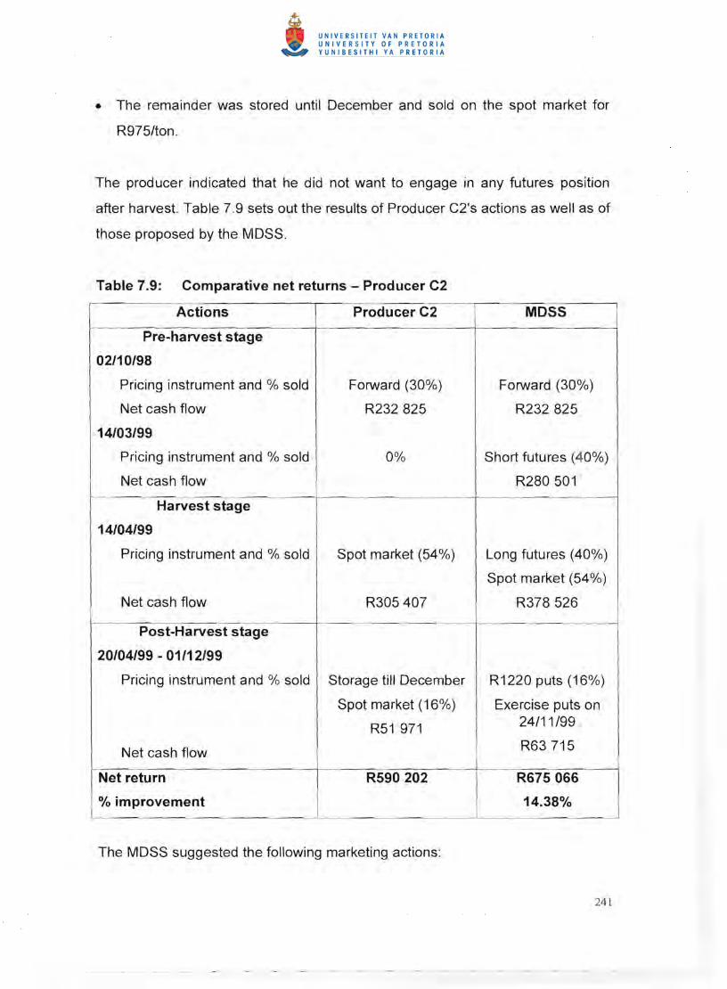
• The remainder was stored until December and sold on the spot market for

R975/ton.

The producer indicated that he did not want to engage in any futures position

after harvest. Table 7.9 sets out the results of Producer C2's actions as well as of

those proposed by the MOSS.

Table 7.9: Comparative net returns - Producer C2

Actions Producer C2 MDSS

Pre-harvest stage

02/10/98

Pricing instrument and % sold Forward (30%) Forward (30%)


14/03/99



Harvest stage

14/04/99


Spot market (54%)


Post-Harvest stage

20/04/99 - 01/12/99

Pricing instrument and % sold Storage till December R1220 puts (16%)

Spot market (16%) Exercise puts on

R51 971 24/11/99


Net return R590202 R675 066

% improvement 14.38%


241

Pre-harvest stage

• 30% of the expected crop was to be sold on 2 October 1998 with a forward

contract at a price of R 1 250/ton.

• Five short futures contracts were to be taken on 14 March 1999 at a price of

R1 200/ton.

Harvest stage

• The short futures position was to be closed on 14 April 1999 with long futures

contracts at a price of R 1 050/ton and the crop was sold on the spot market.

Post-Harvest stage

• Two December put option contracts were to be bought on 20 April 1999 with

a strike price of R 1 220/ton and the contract was to be exercised just before

the expiry date of 24 November 1999.

The MOSS provided better results than both producers. The MOSS was

successfully developed for sunflower seed producers. Although the choice of

marketing instruments was limited by Producer C2, the MOSS could still improve

on the return by 14.38%. If producers use a greater variety of marketing

instruments, not only forward contracts, producers could ensure higher returns .

This proves the importance of using of futures and derivative contracts.

7.5.1.4 Soybean producers

It is important to bear in mind that there are no futures contracts for soybeans in

South Africa. Due to the fact that South Africa is a net importer of soybeans, the

South African price closely follows import parity prices for soybeans. Because

242

no SAFEX marketing alternatives are available to producers, the MOSS can only

suggest the same marketing actions as those followed by the producers.

• Producer 01


Province. Producer 01 planted 105 hectares of soybeans with a realised yield of

2.23 tons per hectare (classified in Category A). The producer engaged in the


• On 1 March 1999, he entered into a forward contract to deliver 100 tons of

soybeans to a local buyer at a price of R 1 200/ton .

• He sold the remainder of his crop on the spot market during harvest,

receiving a price of R1 050/ton.

There was no forward contract available to the producer between the date that

he entered into the contract and his harvest date. The MOSS did not suggest

any other marketing action and the results obtained by the MOSS were thus

obviously the same as those of Producer 01 . The net return of Producer 01's

actions (endorsed by the MOSS) is reflected in Table 7.10.

243



Pre-harvest stage

01103/99


Net cash flow

Forward (42.7%)

R49761

Forward (42.7%)

R49761

Harvest stage

01/05/99


Net cash flow

Spot market (57 .3%)

R42756

Spot market (57.3%)

R42756

Net return

% improvement

R92517 R92514

0%

The MOSS followed exactly the same actions as the producer, due to the fact

that the MOSS could not propose any other marketing instruments.

• Producer 02


Province. Producer 02 planted 550 hectares of soybeans with a realised yield of

2.3 tons per hectare (classified in Category 8). The producer engaged in the


• On 1 December 1998, he entered into a forward contract to deliver 380 tons

of soybea ns at a price of R 1 1 OO/ton.

• He sold 630 tons of his crop on the spot market, receiving a spot price of

R1 050/ton .

• The remainder of his crop was stored until 1 December 1999 and sold on the

spot market at a price of R1 300/ton.

244

The producer could enter into a forward contract during the latter half of March

for a price of R1 200/ton. The producer expected higher spot prices and

declined the offer. The net returns of Producer D2's actions and of those

proposed by the MOSS are reflected in Table 7.11

Table 7.11 : Comparative net returns - Producer 02

MOSS

Pre-harvest stage

Actions Producer 02

01/12/98

Forward (30%) Forward (30%)

Net cash flow


R215774 R215774

23/03/99

0% Forward (40%)

Net cash flow


R155348

Harvest stage

12/05/99

Spot market (10%)

Net cash flow

Pricing instrument and % sold Spot market (50%)

R232466 R122 118

Post-harvest stage

20/05/99 - 01/12/99

Pricing instrument and % sold Storage until Storage until December December

Spot market (20%) Spot market (20%)

R134952 R134952Net cash flow


% improvement 7.72%

The higher return obtained by the MOSS was due to the fact that the producer

disregarded the forward contract presented to him at a later stage.

245

• Producer 03


Province .. Producer 03 planted 525 hectares of soybeans with a realised yield of

4 tons per hectare. Producer 03 was classified in Category C because the total

production volume of soybeans is 2 100 tons. Producer 03 produced soybeans

under irrigation, which explains the higher yield . The producer engaged in the


• On 2 November 199B, he entered into a forward contract to deliver 1 200 tons

of soybeans to a local buyer at a price of R1 100/ton.

• He sold the remainder of his crop (900 tons) on the spot market during

harvest, receiving a price of R1 OBO/ton.

No further forward contracts were available to the producer between the date

when he entered into the contract and his harvest date. The MOSS did not

suggest any other marketing action and the results obtained by the MOSS are

the same as those of Producer 03. The net return of Producer 03's actions is

reflected in Table 7.12.

246



Pre-harvest stage

02/11/98


Net cash flow

Forward (57%)

R392700

Forward (57%)

R392700

Harvest stage

01/05/99


Net cash flow

Spot market (43%)

R276525

Spot market (43%)

R276525

Net return

% improvement

R669225 R669225

0%

From the above examples one can deduce that an MDSS cannot yet

successfully be developed for soybean producers in South Africa. The only

application for the MDSS so far is that producers can use the model to hedge

their crops on the Chicago Board of Trade (CBOT). The usefulness of hedging

on the CBOT has, to date, not yet been established, mainly due to the fact that

South Africa is not a soybean exporter and the spot prices reflect the import

parity prices of soybeans. The I\IIDSS might become more applicable once the

total soybean production in South Africa exceeds the total consumption of

soybeans and soybean products in this country.

7.1 .5.5 Wheat producers

The MDSS used December futures and options contracts in attempting to

optimise the returns of the producers in the sample. All contracts referred to

represent December contracts, unless a post-harvest action is indicated. In

post-harvest actions, the MDSS used May contracts. The December contracts

247

were used because they reflect the harvesting time of wheat, as with the July

contract for maize.

• Producer E1

The farm unit of Producer E1 is in Statistical Region 29 of the Free State

Province. Producer E1 planted 200 hectares of wheat with a realised yield of 2

tons per hectare (classified in Category A) . The producer engaged in the


• On 2 August 1999, he sold 120 tons of his crop on a forward contract at a

price of R1 200/ton.

• The remainder of the crop was sold on the spot market during harvest,

attaining a price of R1 150/ton.

Producer E1 did not want to participate in any futures contracts or derivative

contracts. Table 7.13 displays the results of Producer E1's actions as well as of

those proposed by the MDSS.

248

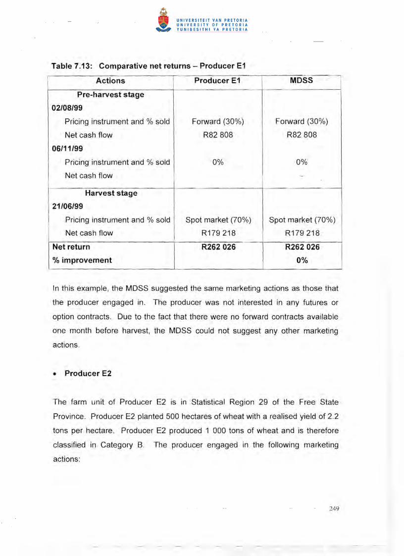
Table 7.13: Comparative net returns - Producer E1

Actions Producer E1 MDSS

Pre-harvest stage

02/08/99


Net cash flow

06/11/99


Net cash flow

Forward (30%)

R82808

0%

Forward (30%)

R82808

0%

-

Harvest stage

21/06/99


Net cash flow

Spot market (70%)

R179218

Spot market (70%)

R179218

Net return

% improvement

R262 026 R262 026

0%

In this example, the MOSS suggested the same marketing actions as those that

the producer engaged in. The producer was not interested in any futures or

option contracts. Due to the fact that there were no forward contracts available

one month before harvest, the MOSS could not suggest any other marketing

actions.

• Producer E2


Province. Producer E2 planted 500 hectares of wheat with a realised yield of 2.2

tons per hectare. Producer E2 produced 1 000 tons of wheat and is therefore

classified in Category B. The producer engaged in the following marketing

actions:

249

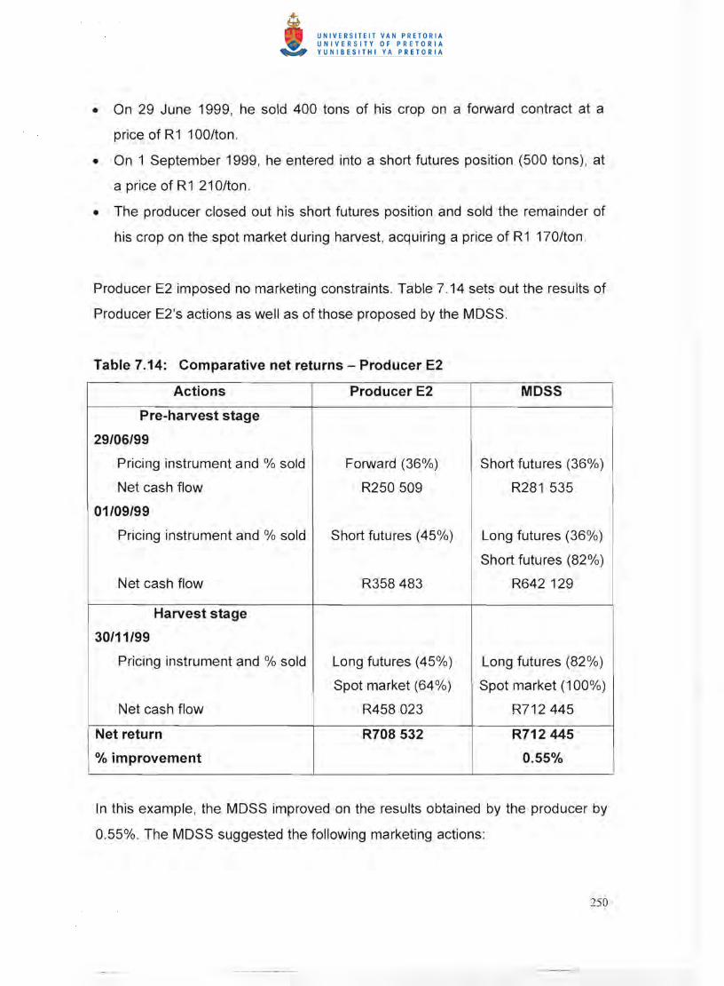
• On 29 June 1999, he sold 400 tons of his crop on a forward contract at a

priceofR1100/ton.

• On 1 September 1999, he entered into a short futures position (500 tons), at

a price of R1 210/ton.

• The producer closed out his short futures position and sold the remainder of

his crop on the spot market during harvest, acquiring a price of R1 170/ton.

Producer E2 imposed no marketing constraints. Table 7.14 sets out the results of

Producer E2's actions as well as of those proposed by the MOSS.


Actions Producer E2 MOSS

Pre-harvest stage

29/06/99


Net cash flow

01/09/99


Net cash flow

Forward (36%)

R250509

Short futures (45%)

R358483

Short futures (36%)

R281 535

Long futures (36%)

Short futures (82%)

R642129

Harvest stage

30/11/99


Net cash flow

Long futures (45%)

Spot market (64%)

R458 023

Long futures (82%)

Spot market (100%)

R712445

Net return

% improvement

R708532 R712445

0.55%

In this example, the MOSS improved on the results obtained by the producer by

0.55%. The MOSS suggested the following marketing actions:

250

Pre-harvest stage

• Four short futures contracts were to be purchased on 29 June 1999 at a price

of R1 189/ton.

• The short futures contracts were to be closed out on 1 September 1999 and a

short position was to be taken for nine December 1999 contracts at a price of

R1210/ton.

Harvest stage

• The short futures position was to be closed out and the crop was sold on the

spot market during harvest.

No marketing action was suggested for 30 October 1999 (one month prior to

harvest) because 82% of the expected crop had already been committed.

• Producer E3


Province. Producer E3 planted 800 hectares of wheat with a realised yield of 2.6

tons per hectare (classified in Category C). The producer engaged in the


• On 10 August 1999, he sold 1 000 tons of his crop on the futures market at a

price of R1 200/ton .

• On 4 November 1999, he closed out his futures position at R 1 180/ton.

• During harvest he sold 1 300 tons of wheat on the spot market, obtaining a


• The remainder of the crop was stored until 15 May 2000 and sold on the spot

market, acquiring a price of R1 250/ton.

251

Producer E3 imposed no marketing constraints . Table 7.15 sets out the results of

Producer E3's actions as we" as of those proposed by the MOSS.



Pre-harvest stage

10108/99


Net cash flow

04/11/99


Net cash flow

Short futures (48%)

R304156

Long futures (48%)

R15932

Short futures (48%)

R304156

Long futures (48%)

R15932

Harvest stage

04/12/99


Net cash flow

Spot market (62%)

R949319

Spot market (100%)

R1575515

Post-harvest stage

10/12/99 - 15/05/00


Net cash flow

Storage

Spot market (38%)

R591 918

Long futures (38%)

Short futures (38%)

R16800

Net return

% improvement

R1 557 169 R1 608247

3.28%

The MOSS achieved an improvement of 3.28% on the producer's actions. The

MOSS suggested the following marketing actions:

Pre-harvest stage

• A short futures position was to be taken on 10 August 1999 on ten December

wheat contracts at a price of R1 200/ton .

252

• The short futures position was to be closed out on 4 November 1999 at a


Harvest stage

• The entire crop was to be sold on the spot market at a price of R1 150/ton.

Post-Harvest stage

• A long futures position was to be taken on eight May 2000 wheat contracts on

10 December 1999 at a price of R1 296/ton .

• The long futu res position was to be closed out at a price of R 1 32 Olton on 15

May 2000.

The MOSS could not improve on the net return of Producer E1. Producer E1 was

not interested in any derivative contract, therefore the same net return was

achieved. The MOSS obtained better returns for both Producer E2 (0.55%) and

Producer E3 (3.28%). It can therefore be declared that the MOSS was

successfully developed for wheat producers in South Africa.

7.6 SUMMARY

When one compares the results obtained using the MOSS with the results

obtained by the individual producers, the following conclusions can be drawn:

• White maize producers: The MOSS produced better results than the

individual producers did in Categories A, Band C.

• Yellow maize producers: The MOSS produced better results in Categories A

and B, but failed to produce better results in Category C. Producer B3

received a spot market price of R45/ton more than the prevailing futures

price.

253

determining the net returns of the marketing actions taken. Cross-hedging

alternatives should be investigated to ensure better price risk management

for crops not traded on SAFEX.

• The MOSS also improved the results of producers already participating on

SAFEX. Producer A3's return was improved by 43.24%, Producer E2's return

was improved by 0.55% and producer E3's return was improved by 3.28% .

This indicates that the MOSS was also successfully developed even for

producers making use of a wider variety of marketing instruments.

In order to manage price risk effectively, producers should use more than one

type of marketing instrument. Producers should strive to secure marketing

instruments that protect them from downside price movements, but also provide

opportunities to participate in an upward price movement. It is important for

producers to sell more of the expected crop during the pre-harvest marketing

phase . Prices normally tend to be lower during the harvest period and any pre

harvest decision could enhance the return.

Table 7.16 analyses the sensitivity to risk exposure of the strategies followed by

the producers (marked as +) and the strategies suggested by the MOSS

(marked as ofo) .

258

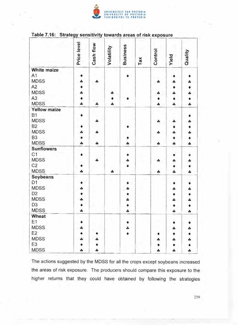
Table 7.16: Strategy sensitivity towards areas of risk exposure

(1) U)~ >> U)0 -(1);;::~ >0-. ~:;; r:::(1) ..r::: "0 -U)U) C'G -r:::~ >< (1)..:(.)

:J:JC'G 00 C'G a.. aJ0 t- O 0~> White maize A1 •• • •MOSS

"'""'"• "'" "'"• "'"•A2 MOSS

"'"• "'"• "'"• "'"• "'" A3 • • MOSS

"'""'" "'" "'" "'" "'" Yellow maize 81 • •MOSS

"'""'" "'"• "'" 82 • ••MOSS

"'" "'" "'" "'" "'"•83 • • • MOSS

"'""'" "'" "'" "'" "'" Sunflowers C1 • • • • MOSS

"'""'" "'" "'" "'"C2 • • ••MOSS

"'""'" "'" "'" "'" Soybeans 01 • • • •MOSS

"'" "'" "'"• "'"02 • • •MOSS

"'""'"• "'"• "'"•03 •MOSS

"'" "'" "'" "'" Wheat E1 • • • •MOSS

"'""'"• "'"• "'" E2 • • ••MOSS

"'""'" "'"• "'" "'" E3 • • ••MOSS

"'" "'" "'" "'" "'" The actions suggested by the MOSS for all the crops except soybeans increased

the areas of risk exposure. The producers should compare this exposure to the

higher returns that they could have obtained by following the strategies

259

suggested by the MOSS. The more complex the strategy, the higher the return

and the more the areas of risk exposure. This therefore requires a constant

revision of the marketing plan. The risk rating of the various marketing actions

was decreased by the fact that the MOSS suggested that about 80% of the crop

must be priced prior to harvesting. Doing so decreased the level of price risk

dramatically.

Marketing is too often an afterthought in the production process. Consequently,

producers are often forced to accept the spot price at harvest in a highly variable

spot market. Thus, price variability in the market translates into price risk, which

compounds with production risk and increases income variability. Effective

management of marketing activities will become increasingly important for farm

business survival as the market becomes more volatile.

7.7 CONCLUSION

This chapter investigated the application of the MOSS developed in Chapter 6.

This chapter shows how producers can manage investment risk with the aid of

an MOSS. While some general conclusions can be drawn from this chapter, they

do not apply to all producers because marketing risk varies across different

crops. Furthermore, price levels and price variability vary from year to year,

depending on market conditions. For example, in years of high planting time

prices, the chances that prices will fall increase, because producers (if weather

allows) may respond to the high prices with a lot of plantings, resulting in an

oversupply of the crop. If the high planting season price is due to short carryover

from the previous year, then the chances of a very high price also increases, due

to the good chance that crops will be in short supply for two years . Producers

need to look at the forward, futures and options markets during planting. They

must consider their own yield potential and variability to understand the degree

260

of investment risk during the marketing season. The MOSS developed in the

previous chapter can be used by producers to customise the results obtained in

this chapter for their own farm conditions and a particular year's price conditions .

261

CHAPTER 8

CONCLUSION AND RECOMMENDATIONS

Nam et ipsa scientia potestas est.

Francis Bacon (1561 - 1626)

8.1 INTRODUCTION

Unfortunately, agricultural producers cannot dictate what price they receive for

their products . The price is determined by the market and, given the transition to

freer global trade and the abolition of the various marketing boards, the market is

likely to become increasingly volatile. All too often, marketing is an afterthought

in the production process. Hence, producers are often forced to accept the price

at harvest. Thus, price variability in the market translates into price risks , which

compound production risks and increase income variability and investment risk.

In future, effective management of marketing activities will become increasingly

important for the survival of any farm business.

Against this backdrop, the overall objective of this study, as formulated in the

introductory chapter, was therefore to develop a marketing decision support

system (an MOSS) for crop producers to manage their investment risk. Decision

support systems are an important application of management information

systems (Davis & Olson, 1985). According to Keen and Morton (1978), decision

support systems imply the use of technology to improve decision-making , and

allow users to retrieve data and evaluate alternatives based on models fitted for

the decisions that have to be made. There are virtually no reports available on

decision support systems for crop marketing in South Africa .

262

8.2 APPROACH FOLLOWED

In order to accomplish the objectives, the following approach was adopted in the

study:

• A critical overview of grain production in South Africa was given. In this

overview the most important crops were established and the deregulation of

the marketing process was discussed.

• Risk management in agriculture was examined. The study also analysed risk

management tools available to producers in South Africa to manage

investment risk.

• The history and application of the futures market in South Africa was

investigated.

• The development and applications of options on futures contracts as viable

risk management tools were investigated .

• A theoretical description, and the development and testing of a proposed

decision support system to aid producers to manage their production risk

were set out.

From this study, a number of conclusions can be drawn, as is set out in Section

8.3 below.

8.3 RESEARCH RESULTS

The aim of the study was to develop a decision support system to help crop

producers to manage investment risk. A postal survey, followed by telephonic

interviews and personal interviews, was conducted during the 1998/1999

marketing season for summer crops and the 1999/2000 marketing season for

wheat, using a sample of grain producers in Statistical Regions 28 and 29 in the

263

Free State Province. Data collected from producers in the Free State were used

in the study for two main reasons . Firstly , there was the overall prominence of

the province (27.3% of the total production) in the production of maize (33.4%),

sunflower seed (54.5%), wheat (43.9%) and soybeans (6 .7%) in South Africa .

Secondly, most of the farming units (18,5%) in South Africa are situated in the

Free State. From the postal survey, a response rate of 28% was obtained . The

postal survey was augmented by telephonic interviews and personal visits . This

resulted in a final response rate of 78%. None of the questionnaires were

unusable due to incomplete information.

The farm units were divided into three different categories. Category A refers to

a farm unit size less than 1000 hectares, the farm unit size for Category B is from

1000 hectares to 1999 hectares, and for Category C, the farm unit size is from

2000 hectares upwards. Due to the fact that the products from farms are not

homogeneous in type and quality, each farm was investigated individually. The

crop choice , input costs and marketing strategies followed by each producer

were compared to the strategies proposed by the model. It was assumed that

producers were hedgers and that obligations from short sales in the futures

market are not satisfied through delivery. Speculation was disregarded in the

testing of the decision support system.

In the testing of the MOSS, the following steps were followed:

• Firstly, the information regarding input costs and marketing strategies

followed by the producer was entered into the programme. Every time when

a producer made a decision, the result was compared to the net effect

suggested by the linear programme. From there on, the decisions suggested

by the linear programme were taken into consideration in future decisions.

For instance, when the programme suggested that the producer should

engage in a short futures position, the futures position would be reflected in

264

the next set of decisions. All option contracts suggested by the model were

at-the-money.

• Secondly, one month prior to harvest, the MOSS was run again to sell a total

of about 80% of the producer's crop. If the producer did sell more than 80%

of the crop one month prior harvest, this action by the MOSS was ignored .

After comparing the results obtained by the MOSS with the results obtained by

the individual producers, the following conclusions could be drawn:

• White maize producers: In all three categories (from 4.8% in Category A to

98% in Category B) the MOSS produced better results than the individual

producers.

• Yellow maize producers: In Categories A (16%) and B (7 .9%) , the MOSS

produced better results, but it reduced the return in Category C (-1.1%) .

• Sunflower seed producers: The MOSS produced better results in both

Categories A (5.6%) and B (14.4%).

• Soybean producers: The MOSS could only improve the results of Category B

(7.7%).

• Wheat producers: The MOSS improved the results of Category B (0.55%)

and C (3.28%) . It failed to improve the results in Category A, due to the

unwillingness of the producer concerned to participate in any SAFEX

contracts.

Table 8.1 shows the individual and average improvement of the MOSS obtained

per crop and per category.

265

Table 8.1: Individual and average improvement using the MOSS

Percentage improvement

Category A Category B Category C Average

White maize 4.8 98.0 43.2 48.7

Yellow maize 16.0 7.9 -1.1 7.6

Sunflower seed 5.6 14.4 10.0

Soybeans 0 7.7 0 2.6

Wheat 0 0.6 3.3 1.3

Average 5.3 25.7 11.3

From the table, some conclusions can be drawn:

• An MOSS has been successfully developed, and producers can apply it

successfully to manage marketing risk and minimise investment risk .

• An MOSS system has been successfully developed for white maize, yellow

maize, sunflower seed and wheat.

• An MOSS system has not yet been developed for crops such as soybeans,

which are not actively traded on the South African Futures Exchange.

• Any size producer, from a small producer to a large producer, can use the

MOSS developed in this study.

• The MOSS developed in this study incorporates all the different marketing

tools available in South Africa to producers to manage their investment risk.

It is the first model developed that implements more than one or two

strategies at a time.

• The MOSS has added value to agricultural risk management in South Africa .

266

8.4 RECOMMENDATIONS AND AREAS FOR FURTHER RESEARCH

This investigation may be regarded as an exploratory step towards the

development of an intelligent decision support system to aid producers to

manage their investment risk. The results by no means provide the final answer

to understanding the complicated processes involved in price risk management.

Within the stated limitations, the findings nevertheless represent, in addition to

obvious financial benefits and implications, a new approach to price risk

management for producers, with direct implications and research opportunities in

the following areas:

• empowering producers with knowledge to make more use of SAFEX in their

quest for price risk management;

• empowering producers to see price risk management as part of total farm risk

management - producers should focus on the farm's risk-bearing capacity

when they develop their marketing plan;

• the proposed model employs very elementary methods for optimising the net

returns of producers, but research in the application of synthetic strategies

must be undertaken;

• tax implications on the net returns of the various strategies should be

investigated;

• daily price changes and their effects on margin accounts were ignored, which

implies that an investigation on daily closing price movements could produce

additional information that should be taken into consideration when

comparing the different marketing alternatives; and

• the proposed model was implemented and tested for one marketing season

only, suggesting that testing the model over a longer period with different

price movements may provide further proof of the viability of the application of

the decision support system.

267

8.5 CONCLUSION

The risks confronted by crop producers are of particular interest, given the

changing role of the government since the 1996 Agricultural Products Marketing

Act was passed. A more sophisticated understanding of risk and risk

management is important to help producers make better decisions in marketing

their produce in the new deregulated environment. An ideal price risk

management tool would cost a small amount, reduce the chances of low net

returns, and not sacrifice upside price potential. Against this background, the

question posed in this study is whether a decision support system could be

developed to manage investment risk faced by grain producers in the marketing

of their crop. This chapter has provided a summary of the most important

conclusions of this investigation . The important limitations and the implications

of this investigation have also been discussed and the areas that warrant further

research indicated.

Learning from mistakes can be an effective educational tool, but learning from

marketing mistakes may be too costly a lesson. Provided they are used with

sufficient realism, decision support systems can help producers to explore

marketing management matters without having to pay too much for possible

mistakes.

268

THE DEVELOPMENT OF A MARKETING DECISION SUPPORT …

Documents

Transcript of THE DEVELOPMENT OF A MARKETING DECISION SUPPORT …