The Development Of A High Resolution Deep-UV Spatial ...
134
University of South Carolina Scholar Commons eses and Dissertations 6-30-2016 e Development Of A High Resolution Deep- UV Spatial Heterodyne Raman Spectrometer Nirmal Lamsal University of South Carolina Follow this and additional works at: hps://scholarcommons.sc.edu/etd Part of the Chemistry Commons is Open Access Dissertation is brought to you by Scholar Commons. It has been accepted for inclusion in eses and Dissertations by an authorized administrator of Scholar Commons. For more information, please contact [email protected]. Recommended Citation Lamsal, N.(2016). e Development Of A High Resolution Deep-UV Spatial Heterodyne Raman Spectrometer. (Doctoral dissertation). Retrieved from hps://scholarcommons.sc.edu/etd/3422
Transcript of The Development Of A High Resolution Deep-UV Spatial ...

University of South CarolinaScholar Commons
Theses and Dissertations
6-30-2016
The Development Of A High Resolution Deep-UV Spatial Heterodyne Raman SpectrometerNirmal LamsalUniversity of South Carolina
Follow this and additional works at: https://scholarcommons.sc.edu/etd
Part of the Chemistry Commons
This Open Access Dissertation is brought to you by Scholar Commons. It has been accepted for inclusion in Theses and Dissertations by an authorizedadministrator of Scholar Commons. For more information, please contact [email protected].
Recommended CitationLamsal, N.(2016). The Development Of A High Resolution Deep-UV Spatial Heterodyne Raman Spectrometer. (Doctoral dissertation).Retrieved from https://scholarcommons.sc.edu/etd/3422

The Development of a High Resolution Deep-UV Spatial Heterodyne Raman
Spectrometer
by
Nirmal Lamsal
Master of Science
Tribhuvan University, 2008
Submitted in Partial Fulfillment of the Requirements
For the Degree of Doctor of Philosophy in
Chemistry
College of Arts and Sciences
University of South Carolina
2016
Accepted by:
S. Michael Angel, Major Professor
Donna A. Chen, Committee Member
Hui Wang, Committee Member
MVS Chandrashekhar, Committee Member
Lacy Ford, Senior Vice Provost and Dean of Graduate Studies

ii
© Copyright by Nirmal Lamsal, 2016
All Rights Reserved.

iii
Dedication
I dedicate this work to my parents who relentlessly helped me in every step of my
life to achieve my goals.

iv
Acknowledgements
First and foremost, I would like to express my heartfelt gratitude to my advisor Dr.
S. Michael Angel for giving me an opportunity to pursue an excellent research work in his
lab. I am grateful to him for his guidance, support and exceptional supervision throughout
my graduate career, without which I would not have been able to complete the difficult
journey of the graduate program. The knowledge, skills, and thoughtfulness that I have
learned from him will always help me move forward in the future.
I would also like to thank my committee members, Dr. Donna A Chen, Dr. Hui Wang and
Dr. MVS Chandrasekhar for serving on my committee. Their constructive criticism and
feedback helped me be a better researcher.
Thank you to my lab mates in the Angel group, past and present. I would like to start with
Janna Register, she was very friendly and has always been a great help no matter the task
or circumstance. Nate Gomer, thank you for all support and mentoring me early on in my
career. Thanks to Joseph Bonvallet, Alicia Strange, Pattrick Barnet, Josh Hungtington and
Ashely Allen for your support and guidance throughout years. I learned a lot from you and
I feel proud to be a part of such a nice group.
Special thanks go to Dr. Shiv K Sharma, one of our collaborators from the University of
Hawaii for giving me a wonderful opportunity to conduct a significant part of my research
work in his lab. I also owe my sincere gratitude to his student Tayro Acosta for assisting
me throughout my time at the University of Hawaii.

v
Abstract
Raman spectroscopy is a light scattering technique that has a huge potential for
standoff measurements in applications such as planetary exploration because a Raman
spectrum provides a unique molecular fingerprint that can be used for unambiguous
identification of target molecules. For this reason, NASA has selected a Raman
spectrometer as one of the major instruments for its new Mars lander mission, Mars 2020,
in the search for biomarkers that would be the indicators of past or present life. Raman
scattering is strongest at UV wavelengths because of the inherent increase in the Raman
cross section at shorter wavelengths and because of the possibility of UV resonance
enhancement. Thus, a Raman spectrometer for planetary exploration would ideally be a
UV instrument. However, existing UV Raman spectrometers are not optimal to integrate
for planetary exploration because they are large and heavy. Existing UV Raman
spectrometers also offer very low light throughput due to the need for narrow entrance slits
to provide high spectral resolution.
This thesis discusses the development of a new type of Fourier transform (FT)
Raman spectrometer; a spatial heterodyne Raman spectrometer (SHRS), which offers
several advantages for field-based UV Raman applications. The SHRS generates a spatial
interferogram using stationary diffraction gratings and an imaging detector. The SHRS is
lightweight, contains no moving parts, and allows very high spectral resolution Raman
measurements to be made in an exceptionally small package, even in the deep UV.

vi
In this study, for the first time, we developed a SHRS system for deep UV
applications using 244 nm excitation that has a spectral resolution less than 5 cm-1 and a
spectral bandpass of 2600 cm-1. Raman spectra of several liquid and solid compounds were
measured using a 244 nm laser to demonstrate the spectral resolution and range of the
system. The SHRS has a large entrance aperture and wide collection angle, which was
shown to be beneficial for the deep UV measurements of photosensitive materials like
NH4NO3 by using a large laser spot size with low laser irradiance on the sample. This is
not possible using conventional UV Raman systems where the need to focus the laser on
sample often leads to photodecomposition. In addition, the use of deep-UV excitation to
mitigate fluorescence was demonstrated by measuring Rh6G, a highly fluorescent
compound, in acetonitrile solution. We also evaluated the performance of the SHRS for
standoff Raman measurements in ambient light conditions using pulsed lasers and a gated
ICCD detector. Standoff UV and visible Raman spectra of a wide variety of materials were
measured at distances of 3-18 m, using 266 nm and 532 nm pulsed lasers, with 12.4” and
3.8” aperture telescopes, respectively. We observed that the wide acceptance angle of the
SHRS simplifies optical coupling of the spectrometer to the telescope and makes alignment
of the laser on the sample easier. More recently, we improved the SHRS design by
replacing the cube beamsplitter with a custom-built higher quality plate beamsplitter,
designed to operate in the range of 240-300 nm, with higher transmission, higher surface
flatness and better refractive index homogeneity. The new design addresses two major
issues of the previous UV SHRS design, namely, optical losses and poor fringe visibility;
as a result, the Raman spectra obtained with new design have much higher signal to noise
ratio than the measurements made using previous design.

vii
Table of Contents
Dedication .......................................................................................................................... iii
Acknowledgements ............................................................................................................ iv
Abstract ................................................................................................................................v
List of tables .........................................................................................................................x
List of figures ..................................................................................................................... xi
Chapter 1. General Discussion of Deep UV Raman Spectroscopy .....................................1
1.1 Introduction ........................................................................................................1
1.2 Raman Theory ....................................................................................................2
1.3 Raman Instrumentation ......................................................................................3
1.4 UV Raman Spectroscopy ...................................................................................7
1.5 References ..........................................................................................................9
Chapter 2. Spatial heterodyne Raman spectroscopy ..........................................................14
2.1 Introduction to Interferometry .........................................................................14
2.2 Theoretical Consideration to Interferometry ...................................................15
2.3 Spatial Heterodyne Raman Spectrometer ........................................................17
2.4 References ........................................................................................................29
Chapter 3. Deep-UV Raman Measurements Using a Spatial Heterodyne Raman
Spectrometer (SHRS).............................................................................................33
3.1 Abstract ............................................................................................................33
3.2 Introduction ......................................................................................................34
3.3 Experimental ....................................................................................................35
3.4 Results and Discussions ...................................................................................38

viii
3.5 Conclusions ......................................................................................................47
3.6 Acknowledgements ..........................................................................................47
3.7 References ........................................................................................................48
Chapter 4. Standoff Spatial Heterodyne Raman Spectroscopy .........................................61
4.1 Background ......................................................................................................61
4.2 Standoff Raman system Instrumentation Overview ........................................62
4.3 Geometry of Collection optics .........................................................................63
4.4 Standoff system coupling .................................................................................64
4.5 References ........................................................................................................65
Chapter 5. UV Standoff Raman Measurements Using a Gated Spatial Heterodyne Raman
Spectrometer ..........................................................................................................69
5.1 Abstract ............................................................................................................69
5.2 Introduction ......................................................................................................70
5.3 Experimental ....................................................................................................72
5.4 Result and Discussions ....................................................................................75
5.5 Conclusions ......................................................................................................82
5.6 Acknowledgements ..........................................................................................82
5.7 References ........................................................................................................83
Chapter 6. Performance Assessment of a Plate Beamsplitter for Deep-UV Raman
Measurements with a Spatial Heterodyne Raman Spectrometer ...........................93
6.1 Abstract ............................................................................................................93
6.2 Introduction ......................................................................................................94
6.3 Experimental ....................................................................................................95
6.4 Results and Discussions ...................................................................................98
6.5 Conclusions ....................................................................................................106
6.6 Acknowledgements ........................................................................................106
6.7 References ......................................................................................................107

ix
Appendix A: Permission to Reprint Chapter 3 ................................................................118
Appendix B: Permission to Reprint Chapter 5 ................................................................119

x
List of Tables
Table 3.1. The table shows the change in interferogram cross section, fringe visibility (FV)
and band intensity of Hg 254.5 nm (39370 cm-1) line with the increase in Littrow
wavenumber .......................................................................................................................50

xi
List of Figures
Figure 1.1. Energy level diagram showing energy transitions for Rayleigh and Raman. The
energy changes that produce stokes and anti-Stokes emissions are depicted on the right.
The two differ from the Rayleigh radiation by frequencies corresponding to νm, the energy
of the first vibrational level of the ground state .................................................................12
Figure 1.2. Raman Spectra of argenine using 532nm (top) and 244 nm laser excitation, and
phenylalanine (lower) using 244 nm laser excitation. The spectra were measured in Angel’s
lab .......................................................................................................................................13
Figure 2.1. Optical layout of a spatial heterodyne Raman spectrometer ...........................31
Figure 2.2. Optical layout that shows the working principle of SHRS. For specific
wavelength, λ, figure on top (A) corresponds to the Littrow configuration in which angle
of incidence will be equal to the angle of diffraction and no interference pattern is formed.
But for any wavelength other than λ, figure on the bottom (B) diffraction occurs and
crossed wavefront is formed resulting into interference pattern which on Fourier
transformation gives intensity spectrum ............................................................................32
Figure 3.1. Spatial heterodyne Raman spectrometer system layout for UV Raman
measurements, with symbols meaning: (M) Mirror, (NF) notch filter/ laser rejection filter,
(I) iris/aperture, (BS) beamsplitter, (G) grating, (IL) imaging lens and (CCD) charge
coupled device. The sample was illuminated with the 244 nm laser incident on the sample,
at 150o with respect to the collection lens optical axis ......................................................51
Figure 3.2. Schematic of a spatial heterodyne spectrometer used for Raman measurements.
S= scattered light, L=lens, CL= collimated light, E= entrance aperture, G= grating; BS=
beam splitter; CW= crossed wavefronts exiting the SHRS ...............................................52
Figure 3.3. SHRS Raman spectrum of diamond shown is the Fourier transform of the
interferogram (I) cross section, which is formed by summing the intensity of each column
of pixels in the fringe image (FI). The spectrum was acquired using 13 mW, 244 nm
excitation, 60 second integration time and Littrow set to 1300 cm-1 ................................................53
Figure 3.4. SHRS Raman spectra of (A) Teflon, (B) potassium perchlorate and (C) calcite
measured using the SHRS spectrometer with Littrow set to ~590 cm-1. The arrows above
each spectrum refer to the appropriate intensity axis for that spectrum. The other
parameters include integration time 60 seconds, 244 nm excitation and 5 mW laser power
at the sample. Spectra are offset vertically for clarity .......................................................54
Figure 3.5. SHRS Raman spectrum of acetonitrile and interferogram fringe image cross
section (top inset). The spectrum was acquired with the sample in a 1 cm quartz cuvette
using 244 nm excitation and 13 mW laser power at the sample with 60 second exposure

xii
time. Dashed line: instrument response function for the SHRS system. The SHRS
instrument response function was determined by measuring the 253.5 nm Hg emission line
intensity (filled circle) as a function of Littrow wavelength and fitting a polynomial curve
to the resultant response .....................................................................................................55
Figure 3.6. SHRS Raman spectrum of acetonitrile acquired by collecting three separate
spectra using Littrow settings of ~700 cm-1, ~2800 cm-1 and 2800 cm-1, and stitching the
resultant spectra together. Each spectrum was acquired using 244 nm excitation, 5 mW
laser power and 60 second exposure time with the samples placed in 1 cm quartz
cuvette ................................................................................................................................56
Figure 3.7. SHRS Raman spectra of sodium sulfate for (A) focused (30 μm diameter) and
(B) unfocused (2500 μm) laser spots on the sample. The spectra were obtained using 244
nm excitation, 5 mW laser power at the sample and 60 second exposure time with Littrow
setting to ~600 cm-1 ...........................................................................................................57
Figure 3.8. SHRS Raman spectra of ammonium nitrate for (A) focused (25 μm diameter)
and (B) unfocused (1500 μm) laser on the sample. The spectra were acquired using 244 nm
excitation, 5 mW laser power at sample and 60 seconds exposure time with Littrow set to
670 cm-1 .............................................................................................................................58
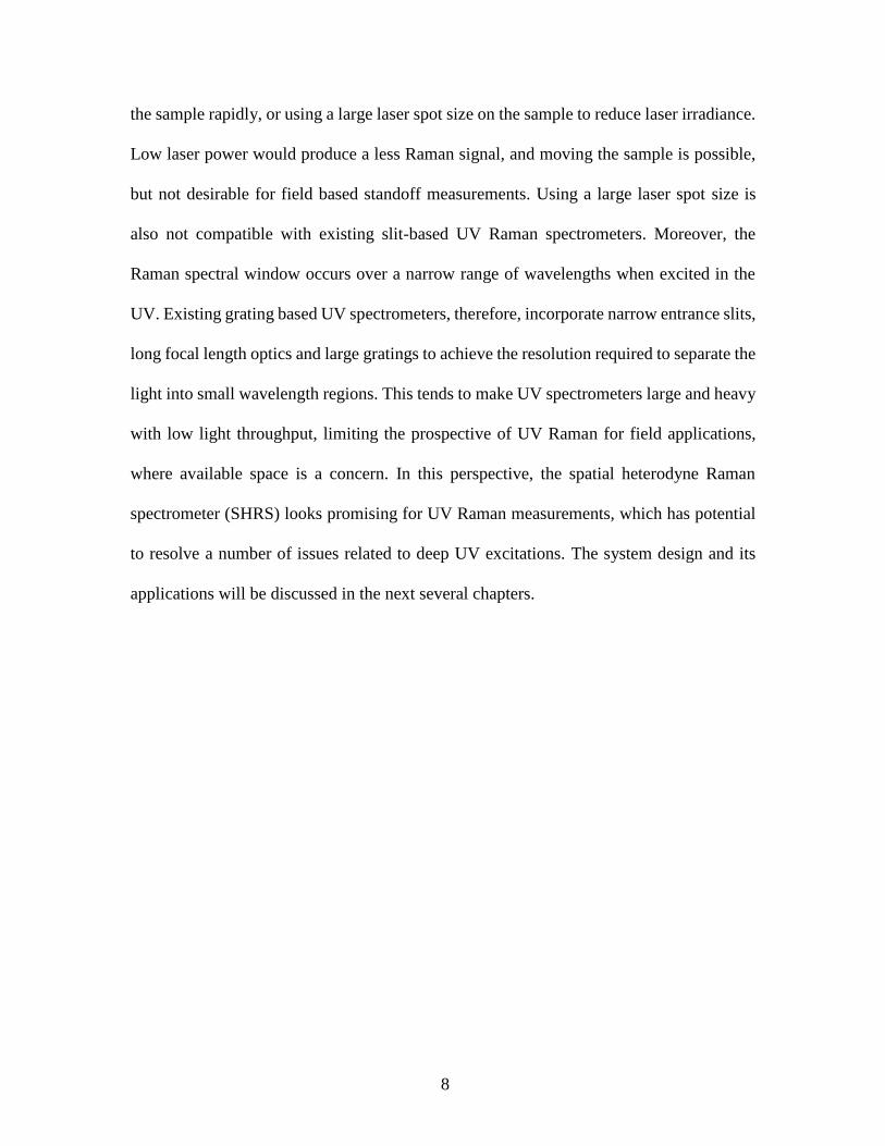
Figure 3.9. SHRS Raman spectrum of acetonitrile spiked with 1.45 ppm Rhodamine 6G.
The spectra were acquired using 244 nm excitation, 5 mW laser power at the sample and
60 second exposure time with the Littrow set to ~2000 cm-1. A 300 nm short pass optical
filter was used to block fluorescence .................................................................................59
Figure 3.10. UV excited fluorescence spectrum of 1.45 ppm Rhodamine 6G in acetonitrile,
measured using ocean optics spectrometer (Model: USB4000-UV-VIS) The dashed line
shows the transmission profile of the 300 nm short pass filter that was used to acquire the
UV Raman spectrum shown in Fig. 9. Other parameters include 244 nm excitation, 5 mW
laser power at sample and one second acquisition time ....................................................60
Figure 4.1. Typical optical system schematic for a standoff Raman spectroscopy ...........67
Figure. 4.2. Schematic of standoff Raman system showing (A) co-axial, used for UV
excitation, and (B) oblique, used for visible excitation, geometries for laser and telescope
optical paths .......................................................................................................................68
Figure 5.1. Schematic of standoff Raman system showing (a) co-axial, used for UV
excitation, and (b) oblique, used for visible excitation, geometries for laser and telescope
optical paths. Note: coupling optics for UV telescope are not shown ...............................86
Figure 5.2. Detailed schematic showing the layout and illustrating the working principle of
the SHRS. S=light from sample, CL=collection lens, E=entrance aperture, IW=input
wavefront, BS=beamsplitter, G=diffraction grating, CW=crossed wavefronts, IL=imaging
lens, θL=Littrow angle ........................................................................................................87
Figure 5.3. UV standoff Raman spectra of (a) potassium chlorate, KClO3 (b) urea, (c)
calcite, and (d) potassium perchlorate, KClO4 at ~18 m, measured using the SHRS

xiii
spectrometer with Littrow set to ~600 cm-1. The arrows above each spectrum refer to the
appropriate intensity axis for that spectrum. Spectra were measured using 10.3 mJ/pulse,
10 Hz pulse rate, 266 nm laser pulses with a total integration time of 60 s. Spectra are offset
vertically for clarity............................................................................................................88
Figure 5.4. Teflon interferogram fringe image (top inset), intensity cross-section (middle
inset) and Raman spectrum for sample at ~18 m, obtained using the SHRS with Littrow set
to ~500 cm-1. The spectrum was measured using 10.3 mJ/pulse, 10 Hz pulse rate, 266 nm
excitation laser pulses with a total integration time of 60 s ...............................................89
Figure 5.5. Visible standoff Raman spectra of (a) NH4NO3, (b) TiO2, and (c) sulfur at 3, 10
and 14 m, with 62, 103 and 106 mW laser power at the samples, respectively, and 60 s
integration time. The spectra were measured using a 532 nm pulsed laser operating at 20
Hz. The Littrow wavelength was different for each sample and is given in the text. The
inset shows the fringe image and cross section of sulfur. The arrows above each spectrum
refer to the appropriate intensity axis for that spectrum. Spectra are offset vertically for
clarity .................................................................................................................................90
Figure 5.6. SHRS Raman spectra of diamond measured in triplicate, using 16 mW, 244 nm
CW laser with 0.5 s and 60 s exposure times, with SHRS mounted on floating (F) and non-
floating (NF) optical table. Twelve total spectra are shown in this plot. The triplicate
measurements overlap to the extent that they cannot be discerned, indicating vibrational
stability in the SHRS during the time required to make the measurements ......................91
Figure 5.7. SHRS Raman spectra of sulfur at 10 m standoff distance recorded using 20, 60
and 1200, 532 nm laser pulses, 5.3 mJ/pulse and 20 Hz pulse rate with 9.6 cm diameter
collection optics .................................................................................................................92
Figure 6.1. Schematic of the spatial heterodyne Raman spectrometer. (S) Light source,
(CL) Collection/collimated lens, (LF) Laser rejection filter, (IA) Iris/Input Aperture, (BS)
Beamsplitter, (CP) Compensator plate, (G) Grating, (IL) Imaging lens .........................109
Figure 6.2. SHRS Raman spectrum of diamond measured illuminating 10 mw 244 nm laser
for 10 s with improved SHRS design. The interferogram image and its cross section are
shown in the inset. The Littrow was set at 1050 cm-1 ......................................................110
Figure 6.3. The SHRS Raman spectrum of Na2SO4 spectrum, which is the Fourier
transform of the image cross section intensity shown in top inset. The integration time is
10 s with 244 nm 8mW laser power at the sample and Littrow is ~500 cm-1.................. 111
Figure 6.4. Raman spectra of rocks and minerals with major constituents of (A) Gypsum,
(B) Quartz, (C) calcite, (D) snail shell. The spectra were obtained by illuminating 10 mW,
244 nm laser at the samples for 30 seconds. The major Raman peak of each samples are
labelled .............................................................................................................................112
Figure 6.5. Raman Spectra of Teflon measured using 244 nm laser excitation with the
SHRS of two different designs (A) with plate BS (B) with cube BS. The experimental
conditions including the laser power (5 mW), acquisition time (30 s) and Littrow position

xiv
(~700 cm-1) were same for both measurements. Figure (C) and (D) show the corresponding
interferogram fringe image and the image cross section for plate BS and cube BS
respectively ...................................................................................................................... 113
Figure 6.6. A plot showing the effect of fringe visibility of an interferogram on the SNR of
reconstructed spectrum. The plot was obtained by recording the interferogram by moving
one of the gratings off from its zero path difference position. The sample was Na2SO4 and
other experimental conditions include 8 mW 244 nm laser and 10 s acquisition time. The
figure in inset shows the change in the 993 cm-1 intensity with fringe visibility ............114
Figure 6.7. Acetonitrile interferograms and Fourier recovered Raman Spectra measured
using SHRS with (A) plate and (B) cube beamsplitter with Littrow set close to 800 cm-1.
The two measurements were carried out in different experimental conditions. For the
measurement involving a plate beamsplitter, 244 nm 6 mW laser was illuminated on the
sample for 10 s. For the measurement involving a cube beamsplitter, 244 nm 13 mW laser
was illuminated on the sample for 30 s ............................................................................ 115
Figure 6.8. The Raman spectra of acetonitrile generated by partitioning the interferogram
into three symmetrical halves along Y-axis (vertical) and applying a Fourier transform to
each halves individually and correspond to SHRS with (A) a plate beamsplitter (B) a cube
beamsplitter. For the CCD camera with 512 pixels along Y- axis, the top spectrum
corresponds to 512-341 pixels, the middle spectrum corresponds to 341-170 pixels and the
bottom spectrum corresponds to 170-1 pixels .................................................................116
Figure 6.9. SHRS Raman spectrum of cyclohexane measured over (A) wide spectral range
(B) limited spectral range using 254 nm bandpass filter. The spectra were acquired using 9
mW, 244 nm laser with 10 s acquisition time. Inset: the cyclohexane’s interferogram
measured over (C), wide spectral range (D) limited spectral range. The arrows above each
interferograms refer to the appropriate intensity axis for that spectrum. The spectra and
interferogram cross sections are offset vertically for clarity ...........................................117

1
Chapter 1
General Discussion of Deep UV Raman Spectroscopy
1.1 Introduction
The phenomenon of inelastic scattering of light was first discovered by Indian
Professor C. V Raman in 1928,1 for which he was awarded the Nobel Prize in Physics in
1930. Raman spectroscopy is a non-destructive vibrational technique that provides detailed
molecular and structural information of the sample under investigation. The technique is
based on the inelastic scattering of the light, where a photon interacts with matter to
produce scattered radiation at different wavelengths or frequencies. Since, the difference
in frequency corresponds to the vibrational or rotational energy level of a molecule, the
Raman spectrum can be treated as a molecular “fingerprint” and can be used to determine
molecular structure.
Although highly versatile, historically, the technique of Raman spectroscopy was
limited to a few sophisticated research labs and was rarely used for ‘real-world’ chemical
analysis because of fundamental and technical limitations, including extremely weak
Raman intensity, fluorescence interference, and the unavailability of efficient light
collection and detection systems. In recent years, instrumental and technological
developments such as the invention of charge coupled device (CCD) detectors, holographic
optical filters, and efficient spectrometers have led to major improvements in Raman

2
spectrometers. As a result, the technique is widely used today in many applications
including pharmaceutical analysis,2–4 explosive detection,5–10 forensic science,11–13 and
planetary exploration14–19, biochemistry and medical applications etc. Raman is beneficial
for these applications because it is a non-invasive in situ technique that does not require
sample preparation and provides accurate chemical information for the samples in many
forms (gas, liquid or solid state).
1.2 Raman Theory
Raman spectroscopy is an inelastic light scattering technique, in which the sample
is excited from the ground state energy level to a higher, shorter-lived virtual state by
illuminating with a monochromatic light source, typically a laser with wavelength λo or
frequency νo. Most light scattering take place with no loss in energy, and therefore no
frequency (νo). This is known as Rayleigh or mie scattering. However, a very small fraction
of light (1 in every 106-108 photons)20 scatter with a loss of energy to the molecule and this
is known as Raman scattering. As illustrated in Fig. 1.1, Raman scattered photons are
shifted in frequencies (i.e. Raman shift) because the excitation photon energy is either
transferred to or received from the sample, as a result of a change in vibrational or rotational
modes of the molecules in the sample. Photons with lower energy (νo – νm) than the incident
photon are known as Stokes Raman photon, while the photon with higher energy (νo + νm)
are known as anti-Stokes Raman photons. Raman spectra are plotted as scattered light
intensity versus Raman shift, (Δ cm-1), the energy difference between the laser photons and
the Raman scattered photons. Elastically scattered light is removed using a combination of
extremely narrow band notch filters and proper design of the spectrograph.

3
Although IR and Raman are both vibrational “fingerprint” techniques, the selection
rules are different. Raman requires a change in molecular polarizability while IR requires
a change in the dipole moment during a normal mode of vibration. Due to the different
selection rules, many molecules, which are not IR active such as H2, N2, and O2, which can
be measured using Raman spectroscopy. By the same token, Raman spectroscopy can be
used to measure bands of symmetric linkages such as -S-S-, -C-S-, -C=C-, which are weak
in an infrared spectrum.20
1.3 Raman Instrumentation
A typical Raman system consists of four major components: a monochromatic light
source to excite the sample, filtering and collection optics to collect the scattered light of
specific interest, a spectrometer to disperse the light into its spectral components, and a
detector to record the spectrum. In the following section, each of the components are
described in detail.
1.3.1 Excitation Source
Since Raman cross sections are very low, a powerful light source is required to
produce sufficient Raman scattered photons. Although the first Raman measurements were
made using sunlight,1 all modern Raman spectrometers use lasers exclusively as the light
source. Lasers are ideal for Raman spectroscopy because they are highly monochromatic,
possess low divergence, and are therefore easy to collimate, can provide high power density
on the sample and most importantly are available in the wavelength regions ranging from
UV to IR. Both CW and pulsed lasers are used for Raman. Pulsed lasers combined with
gated detectors have been shown to be very effective in eliminating background light while

4
conducting the Raman measurements in ambient light conditions.7 The proper selection of
laser wavelength is a critical for the success of Raman spectroscopy. Raman cross section
is inversely proportional to the fourth power of excitation wavelength (1/ λ4). thus shorter
wavelengths can yield higher Raman signals.21 Therefore, visible wavelengths are most
commonly used in Raman. Also, visible lasers produce relatively high power and are cost
effective. However, a strong fluorescence background, from either the analyte or
impurities, can be a significant problem when using visible excitation. Lower energy NIR
wavelengths reduce the likelihood of fluorescence background but are not very desirable,
because the Raman scattering is inherently weak. Deep-UV excitation can be used to avoid
fluorescence interference, while preserving the sensitivity of the system, as the Raman shift
occurs in a spectral region far from fluorescence wavelengths. The use of UV excitation,
however, is limited to a few applications largely due to laser-induced damage to the sample,
the lack of suitable UV transmissive optics, and larger, more complex, and expensive UV
lasers.
1.3.2 Filtering and Collection optics
With Raman scattering, being a very weak phenomenon, a big part of experimental
effort goes into setting up the excitation and collection optics to gather as much scattered
light as possible. Typically, lenses are used to focus the laser onto the sample and to collect
the scattered radiation. Either a single lens or a combination of lenses can be used to
transfer the light into the spectrometer. Normally, 90o collection geometry is used for
transparent liquids, whereas 180o backscattering collection geometry is typically employed
for opaque samples. The light gathering capacity of a lens is defined in terms of an F-
number (F#), which is the ratio of focal length (f) to diameter (D) of the lens (i.e., F#=f/D).

5
It is necessary to match the F# of the lens with the spectrometer in order to
maximize the optical throughput. Fiber optic cables are also employed to collect light,
mainly in handheld instruments and for online monitoring, and in-situ analysis.22,23 Fiber
optic systems consist of single fiber or multiple fibers, where one fiber delivers the laser to
the sample and adjacent fibers collects and transmit the scattered light into the
spectrometer. In remote Raman measurements, telescopes are employed to compensate for
the decrease in signal due to sample distance. The telescope is coupled to the spectrometer
either through fiber optics or using intermediate lenses.24,25 Standoff measurements are of
great benefit for hazardous samples such as explosives5,7,8,26,27, where direct contact could
be potentially harmful or for planetary exploration,17,19,24 to extend the range over which
the samples are accessible.
Since most of the scattered photons have the same frequency as the laser (Rayleigh
scattering), it is essential to block these photons from entering the system. Usually, notch
filters or long pass filters are incorporated to block laser scattered light while transmitting
Raman scattered light. Notch filters blocks a small wavelength band, a few nanometers
wide, centered on the laser wavelength. This allows both Stokes and anti-Stokes band to
be recorded, while blocking the Rayleigh scattered light.
1.3.3 Spectrometers
The available spectrometers for Raman systems can be divided into two categories;
dispersive grating based spectrometers and Fourier transform interferometers. In dispersive
system, the collected light is first focused onto the entrance slit of the spectrometer, which
is then collimated by a concave mirror or lens and directed to a diffraction grating. The
light is dispersed into its component wavelengths, a small bandpass of which is then

6
allowed to exit towards the detector. The extent of dispersion depends on the gratings
groove density and the focal length of the spectrometer. Although optically efficient, the
tradeoff between the resolution and sensitivity sometimes create difficulty implementing
dispersive spectrometer especially for high-resolution measurements. The Fourier
transform (FT) Raman uses multiplex spectrometer such as Michelson interferometer,
which measure all wavelengths of light simultaneously producing interferogram as output.
The intensity spectrum is then recovered by applying Fourier transformation to the
interferogram. Unlike dispersive spectrometers, the noise from each of the wavelengths are
distributed throughout the spectrum. Therefore, it is essential to block any scattered light
like laser, fluorescence or any out of band light for successful operation of FT
interferometer. FT Raman spectroscopy was first developed by Hirschfeld and Chase28 and
used infrared excitation to avoid fluorescence background. The less energetic IR
excitations were difficult to implement with dispersive spectrometers because of the shot
noise limited detectors29, such as PMT, which had very low quantum efficiency in IR.
1.3.4 Detectors
The charge coupled device (CCD) and the intensified charge coupled device
(ICCD) are the preferred detectors for low light measurements such as for Raman
spectroscopy. Both have a two dimensional array of pixels to store and manipulate the
photons in the form of electrical charges. The choice of the CCD detectors depends on the
excitation wavelength, spectral range, sensitivity and speed of the data acquisition. The
properties that influence the performance of CCD detectors include quantum efficiency,
number of channels, dark noise and readout noise. Most of the modern CCD detectors
possess extremely low thermal and readout noise (i.e., shot noise limited) and have high

7
quantum efficiency from UV to IR. They can also record a full Raman spectrum in a single
measurement, typically without scanning the spectrometer. The two dimensional CDD
array also allows to perform spatial resolution of the sample and can be used to take the
full image of the sample.
1.4 UV Raman Spectroscopy
As stated previously, there are several advantages using UV excitation in Raman
spectroscopy. Short wavelength excitation can provide richest Raman sensitivity, since the
Raman scattering efficiency is proportional to 1/λ4. 21 Also, there is a possibility of
resonance enhancement, which occurs when excitation wavelength is close to the
wavelength of an electronic state within the molecule. Many organic and inorganic
materials show resonance enhancement30,31 up to 106 times when excited in the deep-UV.
As an example of increased sensitivity in the UV, Fig. 2 compares Raman spectra of
argenine measured using both 532-nm and 244-nm excitation. The 244-nm Raman spectral
intensity was 4670 times higher for argenine using 244-nm excitation because of the 1/λ4
scattering efficiency dependence and resonance effects, in addition to lower fluorescence
using UV excitation. In addition to enhanced Raman scattering, fluorescence suppression
is an advantage at deep UV wavelengths, since the Raman spectrum will be shifted to
wavelengths below the longer wavelength fluorescence.32 Fluorescent samples will still
fluoresce, but the fluorescence will appear at wavelengths that are far removed from the
Raman bands and thus the two signals can be completely isolated using optical filters.
There are many practical difficulties and disadvantages using UV for Raman
measurements. A major disadvantage of UV excitation is photo-and thermal-degradation
of the sample. Some solutions to this problem include the use of low laser power, moving
8
the sample rapidly, or using a large laser spot size on the sample to reduce laser irradiance.
Low laser power would produce a less Raman signal, and moving the sample is possible,
but not desirable for field based standoff measurements. Using a large laser spot size is
also not compatible with existing slit-based UV Raman spectrometers. Moreover, the
Raman spectral window occurs over a narrow range of wavelengths when excited in the
UV. Existing grating based UV spectrometers, therefore, incorporate narrow entrance slits,
long focal length optics and large gratings to achieve the resolution required to separate the
light into small wavelength regions. This tends to make UV spectrometers large and heavy
with low light throughput, limiting the prospective of UV Raman for field applications,
where available space is a concern. In this perspective, the spatial heterodyne Raman
spectrometer (SHRS) looks promising for UV Raman measurements, which has potential
to resolve a number of issues related to deep UV excitations. The system design and its
applications will be discussed in the next several chapters.

9
1.5 References
1. C.V. Raman, K.S. Krishnan. “A New Type of Secondary Radiation”. Nature. 1928.
121(3048): 501–502.
2. T. Vankeirsbilck, A. Vercauteren, W. Baeyens, G. Van der Weken, F. Verpoort, G.
Vergote, “Applications of Raman spectroscopy in pharmaceutical analysis”. TrAC
Trends Anal. Chem. 2002. 21(12): 869–877.
3. B. D. Patel, P. J. Mehta. “An Overview: Application of Raman Spectroscopy in
Pharmaceutical Field”. Curr. Pharm. Anal. 2010. 6(2): 131–141.
4. S. Sasic, Pharmaceutical applications of Raman spectroscopy. Wiley-Interscience,
Hoboken, N.J, 2008.
5. K.L. McNesby, R.A. Pesce-Rodriguez. “Applications of Vibrational Spectroscopy in
the Study of Explosives”. In: J.M. Chalmers, P.R. Griffiths, editors. Handbook of
Vibrational Spectroscopy. John Wiley & Sons, Ltd, Chichester, UK, 2006.
6. K.L. McNesby, C.S. Coffey. “Spectroscopic Determination of Impact Sensitivities of
Explosives”. J. Phys. Chem. B. 1997. 101(16): 3097–3104.
7. J.C. Carter, S.M. Angel, M. Lawrence-Snyder, J. Scaffidi, R.E. Whipple, J.G.
Reynolds. “Standoff Detection of High Explosive Materials at 50 Meters in Ambient
Light Conditions Using a Small Raman Instrument”. Appl. Spectrosc. 2005. 59(6):
769–775.
8. S. Sadate. “Standoff Raman Spectroscopy of Explosive Nitrates Using 785 nm Laser”.
Am. J. Remote Sens. 2015. 3(1): 1-10.
9. M.L. Ramírez-Cedeño, N. Gaensbauer, H. Félix-Rivera, W. Ortiz-Rivera, L. Pacheco
Londoño, S.P. Hernández-Rivera. “Fiber Optic Coupled Raman Based Detection of
Hazardous Liquids Concealed in Commercial Products”. Int. J. Spectrosc. 2012.
2012:1–7.
10. G. Tsiminis, F. Chu, S. Warren-Smith, N. Spooner, T. Monro. “Identification and
Quantification of Explosives in Nanolitre Solution Volumes by Raman Spectroscopy
in Suspended Core Optical Fibers”. Sensors. 2013. 13(10): 13163–13177.
11. F.J. Bergin. “A microscope for fourier transform Raman spectroscopy”. Spectrochim
Acta Part Mol. Spectrosc. 1990. 46(2): 153–159.
12. A.H. Kuptsov. “Applications of Fourier transform Raman spectroscopy in forensic
science”. J. Forensic Sci. 1994. 39(2).

10
13. E.G. Bartick, P. Buzzini. “Raman Spectroscopy in Forensic Science”. In: R.A. Meyers,
editor. Encyclopedia of Analytical Chemistry. John Wiley & Sons, Ltd, Chichester,
UK, 2009.
14. National Research Council (U.S.), National Research Council (U.S.), eds. Vision and
voyages for planetary science in the decade 2013-2022. National Academies Press,
Washington, D.C, 2011.
15. Wang, B.L. Jolliff, L.A. Haskin. “Raman spectroscopic characterization of a highly
weathered basalt: Igneous mineralogy, alteration products, and a microorganism”. J.
Geophys. Res. 1999. 104 (E11): 27067.
16. P. Vandenabeele, J. Jehli ka. “Mobile Raman spectroscopy in astrobiology research”.
Philos. Trans. R. Soc. Math. Phys. Eng. Sci. 2014. 372(2030): 20140202–20140202.
17. N. Tarcea, T. Frosch, P. Rösch, M. Hilchenbach, T. Stuffler, S. Hofer, et al. “Raman
Spectroscopy—A Powerful Tool for in situ Planetary Science”. Space Sci. Rev. 2008.
135(1-4): 281–292.
18. S.E. Jorge Villar, H.G.M. Edwards. “Raman spectroscopy in astrobiology”. Anal.
Bioanal. Chem. 2006. 384(1): 100–113.
19. S.M. Angel, N.R. Gomer, S.K. Sharma, C. McKay. “Remote Raman Spectroscopy for
Planetary Exploration: A Review”. Appl. Spectrosc. 2012. 66(2): 137–150.
20. E. Smith, G. Dent. Modern Raman spectroscopy: a practical approach. J. Wiley,
Hoboken, NJ, 2005.
21. R.L. McCreery. Raman spectroscopy for chemical analysis. John Wiley & Sons, New
York, 2000.
22. I.R. Lewis, M.L. Lewis. “Fiber-Optic Probes for Raman Spectrometry”. In: J.M.
Chalmers, P.R. Griffiths, editors. Handbook of Vibrational Spectroscopy. John Wiley
& Sons, Ltd, Chichester, UK, 2006.
23. R.L. McCreery, M. Fleischmann, P. Hendra. “Fiber optic probe for remote
Ramanspectrometry”. Anal. Chem. 1983. 55(1): 146–148.
24. S.K. Sharma. “New trends in telescopic remote Raman spectroscopic instrumentation”.
Spectrochim. Acta. A. Mol. Biomol. Spectrosc. 2007. 68(4): 1008–1022.
25. S.M. Angel, N.R. Gomer, S.K. Sharma, C. McKay. “Remote Raman Spectroscopy for
Planetary Exploration: A Review”. Appl. Spectrosc. 2012. 66(2): 137–150.
26. M. Gaft, L. Nagli. “UV gated Raman spectroscopy for standoff detection of
explosives”. Opt. Mater. 2008. 30(11): 1739–1746.

11
27. J. Moros, J.A. Lorenzo, K. Novotný, J.J. Laserna. “Fundamentals of stand-off Raman
scattering spectroscopy for explosive fingerprinting: Raman scattering spectroscopy
for explosive fingerprinting”. J. Raman Spectrosc. 2013. 44(1): 121–130
28. T. Hirschfeld, B. Chase. “FT-Raman spectroscopy: development and justification”.
Appl. Spectrosc. 1986. 40(2): 133–137.
29. B. Chase. “FT–Raman Spectroscopy: A Catalyst for the Raman Explosion?” J. Chem.
Educ. 2007. 84(1): 75.
30. S.A. Asher. “Ultraviolet Raman Spectrometry”. In: J.M. Chalmers, P.R. Griffiths,
editors. Handbook of Vibrational Spectroscopy. John Wiley & Sons, Ltd, Chichester,
UK, 2006.
31. M. Ghosh, L. Wang, S.A. Asher. “Deep-Ultraviolet Resonance Raman Excitation
Profiles of NH4NO3, PETN, TNT, HMX, and RDX”. Appl. Spectrosc. 2012. 66(9):
1013–1021.
32. S. Asher, C. Johnson. “Raman spectroscopy of a coal liquid shows that fluorescence
interference is minimized with ultraviolet excitation”. Science. 1984. 225(4659): 311–
313.

12
Figure 1.1. Energy level diagram showing energy transitions for Rayleigh and Raman. The
energy changes that produce stokes and anti-Stokes emissions are depicted in the middle
and in the right respectively. The two differ from the Rayleigh radiation with frequencies
corresponding to νm, the energy of the first vibrational level of the ground state.

13
Figure 1.2. Raman Spectra of argenine using 532nm (top) and 244 nm laser excitation, and
phenylalanine (lower) using 244 nm laser excitation. The spectra were measured in Angel’s
lab.

14
Chapter 2
Spatial Heterodyne Raman Spectroscopy
This chapter describes the working principle, design, and development of the spatial
heterodyne spectrometer for Raman measurements. The first part of the chapter discusses
the interferometer and the design considerations of two-beam interferometers. The second
part of the chapter describes the details of various aspects of the spatial heterodyne Raman
spectrometer including resolving power, bandpass, optical throughput and instrumentation.
2.1 Introduction to Interferometry
Interferometry refers to techniques, in which electromagnetic waves, such as light
waves are combined to produce an interference pattern, which contains information about
the original waves. Interferometry is based on the superposition principle, which means
when two oscillating electromagnetic waves with the same frequency interfere with each
other; the resulting pattern at some point in space is determined by the phase or the path
difference between the two waves. 1 If two waves are in phase they will reinforce each
other, and undergo constructive interference; waves that are out of phase will cancel each
other, and undergo destructive interference. An instrument based on this technique is
known as interferometer and has numerous applications in astronomy, spectroscopy,
quantum mechanics, remote sensing, seismology, nuclear and particle physics.1 Although
physicist Thomas Young led the way for interferometry from his double slit experiments

15
performed in 1801, a major breakthrough in interferometry was brought about by Albert
Michelson and Morley in 18872 from their famous failed experiment where they attempted
to detect luminiferous aether using the Michelson interferometer. Their failed experiments
changed the way scientists view the workings of the universe.
The Michelson interferometer is the most widely used interferometer to date and
works by splitting a beam of light into two beams. The light reflects by using two mirrors
back towards the beamsplitter where it recombines to create an interference pattern.
Spectroscopic techniques based on interferometry such as FTIR and FT-Raman3 have
several advantages over conventional grating based spectrometers. Interference
spectrometers enjoy much higher light throughput as they lack an entrance slit, and are
therefore useful to make measurements of faint and extended sources. 4 Additionally,
interferometers measure all wavelengths simultaneously and a high resolving power can
be attained in a very small package, which is rather difficult to achieve in grating based
spectrometer.3
2.2 Theoretical Consideration to Interferometry
Interference is the phenomenon that occurs when the light is combined in space.
The phenomenon can be defined more explicitly using the classical wave theory of light.
Light is an electromagnetic wave made up of oscillating electric and magnetic fields,
however, only electric field (E) is relevant to optics. Even more accurately, it is the field
intensity, or, the time average of the electric field intensity squared, E * E = E2, which is
of most importance in optics. This value, also known as irradiance (I), is actually sensed
by a detector. If we consider two coherent electromagnetic waves, with amplitude E0 and

16
the angular frequency (ω), emanating from two sources very close to each other, then the
electric field of two waves at some point in space would be:
E1 = E0 sin ωt (1)
E2 = E0 sin (ωt +ϕ) (2)
Where, ϕ is the phase difference between two waves. The sum of the combined electric
field during interference is given by,
E = E1 + E2 = E0 sin ωt + E0 (sin ωt +ϕ) (3)
Using the trigonometric identity,
sin 𝐴 + sin 𝐵 = 2 sin(𝐴 + 𝐵)
2cos
(𝐴 − 𝐵)
2
and considering, A= ωt +ϕ, B= ωt, Eq. 3 can be written in the form:
𝐸 = 2𝐸0 cos (𝜙
2) sin (𝜔𝑡 +
𝜙
2) (4)
Then irradiance may be written as,
𝐼 = 𝐸 ∗ 𝐸 = 4𝐸02 𝑐𝑜𝑠2 (
𝜙
2) (5)
Equation 5 shows that the intensity will be maximum, or constructive interference will
occur when ϕ=2mπ, and destructive interference will occur when ϕ = (2m+1) π for any
integer m and zero. In this way, the intensity pattern i.e. bright or dark pattern depends
upon the phase difference between the waves interfering with each other. Since, a path
difference of ‘λ’ corresponds to the phase difference of 2π rad for constructive interference;
equation 5 can also be written in the form of a path difference (δ) between two waves. The
path difference δ is related to phase difference by
𝜙 =2𝜋
𝜆 𝛿 (6)

17
In order to observe a high quality interference fringe pattern between the two beams,
several conditions must be met.1 First the phase difference between the two light beams
should not exceed the coherence length, which will be discussed in detail later. Secondly,
the polarization properties of two light waves must match with each other and thirdly the
relative intensities of the two beams should be close to each other.
2.3 Spatial Heterodyne Raman Spectrometer
2.3.1 General Overview
The spatial heterodyne Raman spectrometer (SHRS) is a type of Fourier Transform
spectrometer, first described by Gomer et al.,5 for visible Raman measurements, and
extended into the deep UV by Lamsal et al.6,7 The goal was to develop a small, lightweight
and high throughput spectrometer with no moving parts that offered the resolving power
required for high resolution UV Raman measurements, and overcome issues in
conventional grating based UV spectrometers, which tend to be rather large and bulky with
low throughput. The SHRS follows the design of the basic spatial heterodyne spectrometer
(SHS) as described by John Harlander.8,9 The basic design of the SHS is similar to a
Michelson interferometer but with tilted diffraction gratings instead of moving mirrors.
There are no moving parts, and like a Michelson interferometer, there is no entrance slit.
The small footprint, large input aperture, and lack of moving parts makes the SHRS ideal
for space applications. The SHRS design also offers other advantages, including high
spectral resolution, equal to the resolving power of the combined diffraction gratings, very
high optical etendue, high resolution in the UV and the ability to do 2D imaging. The SHS
has been utilized for applications like atmospheric sensing,9,10 flame absorption
spectroscopy,11 and infrared spectroscopy.12 The SHS boasts a wide acceptance angle at

18
the gratings, from 1° or 10° using field widening prisms,10 and thus a wide-area
measurement capability. SHRS is also compatible with a pulsed laser and gated detector
and the measurement can be performed in ambient light conditions. The use of pulsed laser
also helps to “freeze out” vibrational instabilities in the SHRS.
The high resolution and high throughput offered by the SHRS design is ideal for
deep-UV Raman spectroscopy where the Raman spectrum covers a very small wavelength
range, thus requiring a high-resolution spectrometer to resolve the Raman bands. Because
of the large acceptance angle, the SHRS allows the use of large laser spots on the sample.
This gives lower laser irradiance and minimizes laser-induced damage caused by focusing
a laser onto the sample; consequently, samples can be illuminated using relatively high
laser power. It is also worth noting that the SHRS has only a weak coupling of resolution
and throughput, and as a result, a high-resolution SHRS instrument can be built in a very
small package, useful for space applications where the instrument size is a concerned.
2.3.2 Spatial Heterodyne Raman Spectrometer Working Principle
The SHRS follows the design of the basic spatial heterodyne interferometer as
described by Harlander,8 modified for Raman applications by the inclusion of holographic
laser line rejection filters (Figure 2.1). Despite the modifications, the SHRS maintains the
advantages of a Fourier Transform interferometer including high light throughput (as there
is no input slit), small size, larger field of view and the multiplex advantage. The use of
stationary diffraction gratings makes the SHRS design free from any moving parts, a
distinct advantage over the Michelson interferometer where a mirror has to be continuously
moved during measurements.

19
During SHRS measurements, the scattered Raman light is collected, collimated and
passed through the entrance aperture and divided into two coherent beams by a 50/50 fused
silica beamsplitter. The two beams are then diffracted by the tilted diffraction gratings back
towards the beamsplitter, where they recombine. The SHRS operates in the Littrow
configuration, that is, the gratings are tilted to a specific angle at which a wavelength of
interest retro-reflects, i.e., the angle of incidence will be equal to the angle of diffraction,
producing a zero optical path difference between the beams and producing no interference
pattern. (Figure 2.2, left). This wavelength of interest is known as the Littrow wavelength,
and grating angle is known as the Littrow angle, which can be calculated using grating
equation,
𝑛 𝜆 = 𝑑(𝑠𝑖𝑛𝛼 + 𝑠𝑖𝑛𝛽) (7)
where n is the order, λ is the desired wavelength, m is grating groove density, α is the angle
of incidence and β is the angle of diffraction. The Littrow angle for specific wavelength λ,
will be
Ɵ𝐿 = 𝑠𝑖𝑛−1 (𝜆
2𝑑) (8)
All wavelengths other than the Littrow wavelength will diffract at a slightly
different angle and will cross each other when combining at the beamsplitter thus
producing an interference pattern (Figure 2.2 right). Since, the extent of diffraction (or
crossing angle between two wavefronts) is directly related to the wavelength of light, for
each wavelength, a unique fringe pattern is formed. The frequency of the fringe pattern is
given by,8–10
𝑓 = 4 (σ − σL) tanθL (9)

20
Where f is in fringes/cm, L is the Littrow wavenumber, is a wavenumber other than the
Littrow wavenumber and ƟL is the Littrow angle. Since, the Littrow angle and Littrow
wavenumber are fixed, any change in input wavenumber will change the fringe spacing in
such a way that bands close to Littrow band will produce wide less frequent fringes, while
bands further from Littrow will have thinner, more frequent fringes. The resultant fringe
pattern is imaged onto the two dimensional array detector, typically a CCD or ICCD
camera,8-10 with the fringe modulation intensity varying along the horizontal axis of the
detector, which also corresponds to the dispersion plane of the gratings. The intensity
distribution of the fringe pattern I(x), for a complex spectrum as a function of detector
position, x, along the dispersion plane of the grating is given by,8–10
𝐼(𝑥) = ∫ 𝐵(σ)[1 + cos8π(σ − σL) 𝑥 tan θL]
∞
0
𝑑σ (10)
where B (σ) is the input spectral intensity at wave number σ. The Fourier transform of I(x)
recovers the power spectrum. Figure 2.2 illustrates the process with a fringe image, the
image cross section and the corresponding power spectrum obtained by applying a one
dimensional Fourier transform to the cross section. The measurement is accomplished
without mechanically scanning or moving any parts of the system. Also, as the Littrow
position can be tuned to any wavenumber by tilting the gratings, the measurements can be
performed at any wavelength.
It is to be noted that light does not propagate as a perfect sinusoidal wavefront but
rather in bundles of wavefronts where the individual wavefronts of light are in phase with
each other only for a specified interval of length, known as the coherence length. The
optimum interference pattern can only be obtained from the superposition of light beams

21
propagating in phase (i.e., from coherent source). The coherence length of light is a
function of the bandwidth of the light,13 which is given by,
𝑙 =𝑐
𝛥𝜈 =
𝜆2
𝛥𝜆 (11)
where l is the coherence length, c is the speed of light, Δν and Δλ are the spectral width in
terms of frequency and wavelength respectively. As Eq. 11 shows, monochromatic sources
like lasers have very long coherence lengths, for example, a 632 nm He-Ne laser with
bandwidth 1GHz has a coherence length of 30 cm. Raman bands are typically broad with
very short coherence lengths, in the range of micrometers. In the SHRS, the path length of
each arm of the SHRS is adjusted to match within the coherence length of the Raman band.
When adjusting the Littrow wavelength, the rotational angle of the gratings must be
matched to the a few hundredths of a degree. A mismatch in the arm lengths can lead to
interferogram fringe distortion and reduction in fringe visibility resulting in retrieval error
and increased noise in the spectrum. The optical path difference between the two arms can
be precisely matched by measuring the white light fringe image, as white light has
extremely short coherence length14 (i.e., in an order of a few microns).
2.3.3 Optical Throughput of the SHRS
The sensitivity of any spectrometer is related to the light throughput. One measure
of light throughput in an optical system is etendue15 (E), defined as E=Ω Al, where Ω is
the collection solid angle of the optical system and Al is the area of the limiting aperture of
the collection system. The etendue provides a good comparison of system sensitivity, since
it describes the maximum collection and throughput of an optical system. In dispersive
spectrometers, the entrance slit often limits the system etendue because of the entrance slit

22
being smaller than the image of the excited region of the sample. For a dispersive
spectrometer, the entrance aperture slit size can range from 10-300 microns wide. Utilizing
the SHRS with a 1-inch aperture would give it a throughput advantage 104 times greater
than a dispersive system with a 10-micron entrance slit. (Calculations shown below). An
f/4 monochromator (very fast for a UV system) with a 10-micron entrance slit has an
optical etendue of ~4.8x10⁻⁵ sr cm2. The basic SHRS design provides a much larger
etendue, where the limiting aperture is the diffraction grating and Ω is defined by the
resolution. Of the system as Ωmax =2π/R. In the case of the SHRS system described below
with R=7500, Ωmax =~8 x10⁻⁴ sr, and E =~5x10⁻³ sr cm2, about two orders of magnitude
larger than the monochromator.
2.3.4 Spectral Resolution and Bandpass
The spectral resolution of the SHRS does not depend on a slit and is not a strong
function of spectrometer size. At a given wavenumber the resolving power, R, is
determined by the total number of grooves illuminated on the two gratings. For the SHRS
incorporating gratings of size W mm with d grooves per millimeter,16
𝑅 = 2 𝑊 𝑑 =𝜆
𝛥𝜆=
𝛥 (12)
In equation 12, λ is the center wavelength (or wavenumber) and Δλ, or, Δ is the smallest
resolvable wavelength difference that can be measured by the spectrometer. For the SHRS
instruments, the resolving power is the same as a diffraction limited dispersion
monochromator with equivalent gratings and an infinitely small slit8 i.e., equal to the total
number of grooves illuminated on the diffraction grating—physically impossible using a
conventional dispersive-grating Raman spectrometer. Thus, small gratings can be used in

23
the SHRS and still give high spectral resolution. For example, a 50-mm diffraction grating
with 600 grooves per mm will produce a resolving power of 30,000 when used in first
order, providing spectral resolution of ~1 cm-1 using a 266 nm excitation laser. This is
much higher than is required for most Raman measurements and demonstrates one of the
key design issues. A moderate resolving power of ~7500 is sufficient to provide spectral
resolution (~ 5 cm-1) over a wide spectral range.
The theoretical maximum band pass of the SHRS is determined by the resolving
power, R, and the number of pixels, N, in the horizontal direction (i.e., x-axis) on the
detector. The Nyquist limit sets the highest frequency that can be measured by the detector
to the frequency that produces N/2 fringes.8 For wavelength (λ), the maximum band pass
of the SHRS can be written as:
𝑅 =𝑁 𝜆
2 𝑅 (13)
For samples related to planetary exploration, a spectral range for a typical Raman
measurement is about 300-3500 cm -1. Using a 244 nm laser, this corresponds to a
wavelength range of ~246 to ~267 nm, for a band pass of ~21 nm. For the measurements
that require a larger spectral range, the bandpass can be extended by using the detector with
more horizontal pixels or by reducing the resolution of the system.
2.3.5 The Significance of Spatial Heterodyne Raman Spectroscopy in Planetary
Applications
It is generally accepted that Raman spectroscopy is useful for planetary missions.
NASA has already selected a Raman spectrometer as one of the major instruments for its
upcoming Mars lander mission, Mars 202017,18 that is proposed to be launched in 2020.
Two Raman spectrometers are being developed for this mission, a visible and a UV

24
spectrometer. UV Raman provides much higher sensitivity than infrared or visible Raman
because of the 1/λ4 dependence of Raman scattering19 (e.g., ~100 times higher signal using
266 nm versus 785 nm excitation), the possibility of resonance Raman enhancement20,21
for highly absorbing molecules, and the relative absence of fluorescence22 in this
wavelength region. However, existing UV Raman spectrometers do not meet the following
necessary criteria to be considered for planetary missions: high spectral resolution (5 cm-1
or better), large spectral band pass (250-3500 cm-1), high sensitivity, small size and low
weight. Dispersive, diffraction grating based, UV Raman systems are inherently large in
order to provide the required spectral resolution, and have a very low light throughput
because of the resolution requirement of small slit widths.
A typical commercial UV spectrometer for Raman applications (e.g., Acton
Model, F/6.7) provides 6.5 cm-1 spectral resolution with a 266 nm laser. The dimensions
are 76x30x20 cm3 and it weighs ~21 kg (46 lbs), without the detector or input optics. The
size of such an instrument is inherent in the design of any dispersive diffraction grating
system because of the requirements of long focal length optics and large gratings to achieve
high spectral resolution. Existing non-dispersive UV Raman systems have very poor
spectral resolution (e.g., tunable filter, FT Raman, Hadamard, coded-aperture, etc.) or are
not compatible with pulsed laser excitation and gated detection. Pulsed excitation and gated
detection have been shown to be essential for daylight Raman measurements.23.
2.3.6 The SHRS Design Considerations
The typical spatial heterodyne Raman spectrometer is comprised of the following
major components: collection and filtering optics, two diffraction gratings, a beamsplitter,

25
imaging or relay optics and a two-dimensional photo detector. The success of the SHRS
operation depends on the careful selection of each of these components.
One of the limitations of interferometer-based spectrometers, including the SHRS,
is the multiplex noise, which comes from signals outside the pass band of interest24 and
must be controlled properly. Therefore, filtering unwanted light is an essential part of
SHRS measurements. For Raman measurements, potential sources of multiplex noises are
scattered laser light, fluorescence, unresolved Raman bands, stray light and grating order
overlap. These sources contribute in background noise, and can also reduce the contrast of
the interference pattern. Laser scattering can be easily controlled using commercially
available Raman edge filters or holographic notch filters. Short pass or bandpass filters are
employed to restrict longer wavelength fluorescence. Band pass filters with a spectral
window in the desire spectral range should be used to eliminate unresolved bands or any
bands out of the spectrometer spectral range.
The beamsplitter is another critical component of SHRS. It is the heart of the
interferometer, and any optical losses in it can result into the poor sensitivity. The ability
of the beamsplitter to transmit and reflect the input light intensity is functionalized by its
efficiency (η),25
𝜂 = 4𝑅𝜆𝑇𝜆 (14)
where, T and R are the transmission and reflectance coefficient of the beamsplitter at
wavelength λ. Equation (14) infers that η =1 only when, Tλ = Rλ= 0.5. Any losses or uneven
ratio of transmission and reflectance decreases the efficiency of the beamsplitter.
Additionally, any deviation in optical qualities like surface flatness, material homogeneity
and the presence of defects may distort the transmitted wavefront. Therefore, it is essential

26
to use a beamsplitter with higher efficiency, good surface flatness and fewer surface defects
in order to observe a high quality interferogram. Beamsplitters can typically be found as
plates or as cubes. For visible applications, cube beamsplitters are preferred because they
are easy to align and are cost effective. But it is rather difficult to find a cube beamsplitter
for deep UV because the cement used for binding the prisms tends to absorb UV light
strongly. In this context, the plate beamsplitter seems to be a good option for UV Raman.
The selection of diffraction gratings is also very important. The gratings disperse
the light. The extent of dispersion controls the resolving power, which in turn affect the
bandpass of the system. The gratings with higher groove density yield greater resolving
power, but that will also reduce the bandpass of the system, therefore, it is required to select
the gratings wisely to achieve the best compromise between the resolution and usable
bandpass. Ideal deep UV Raman applications require a resolution 5 cm-1 and a bandpass of
3500 cm-1. Apart from bandpass and resolution, it is also necessary to block higher
diffraction order from reaching the detector, which may significantly increase the noise of
the system. The gratings and beam splitters must be separated at least by a distance that
will prevent 0-order and 2nd-order diffraction from the grating from entering the beam
splitter For example, for an SHRS with 25.4 mm 150 gr/mm gratings the required minimum
separation is about 300 mm for Raman measurements with 532 nm excitation laser.
The physical properties of the gratings, primarily surface properties, plays a
significant role in the performance of the gratings. Defects such as dust, scratches, pinholes
and unevenness in the gratings lead to unwanted scattering, resulting into higher
background. In addition, irregularities in groove spacing and unevenness in the depth of
the grooves leads to wavefront distortions resulting in poor fringe contrast. Holographic

27
gratings have fewer aberrations than ruled reflection gratings, but holographic gratings are
not usually made with coarse groove spacings. Therefore, while a holographic grating is
the best choice for higher resolution measurements, for measurements that require a large
bandpass, ruled gratings are typically the best available option.
Another important component of the SHRS is imaging lenses or relay optics, which
transfer the fringe image onto the detector. Since the overlap of diffracted wavefronts
occurs virtually in front of each of the gratings, an optic or set of optics is required to
precisely image this plane onto the detector. High quality single or multi-component lens
systems are required to eliminate any optical aberrations and to preserve the integrity of
the interferogram. It is important to note that the lenses have inherent limitations to spatial
resolution of the formed image. The ability of a lens to transfer information from object to
image is defined in terms of the modulation transfer function (MTF), which will be
described in detail in chapter 7. Bands with larger wavenumber shifts produce more closely
spaced fringes. It is critical to use the lenses with the highest MTF to maintain high and
presence of high frequency information in the interferogram
While the spectral resolution is determined by the gratings, the spectral range is
determined by the number of pixels on the CCD or ICCD camera in the SHRS instrument.
A large format CCD camera is needed to build SHRS instruments with high-resolution and
broad spectral coverage. Scientific grade large format CCD cameras such as 2048 × 2048
formats are commercially available. The performance of the CCD camera depends on
quantum efficiency, thermal noise and readout noise. In a thermoelectrically cooled CCD,
thermal noise is very low, and the CCD can be built with unichrome coating for enhanced
UV performance to allow for higher quantum efficiency in the UV region. For field-based

28
measurements, an ICCD detector is ideal, which along with a pulsed laser helps to avoid
ambient light background, and allows so an entire Raman spectrum to be acquired with
each laser pulse. The pulsed laser can also “freeze out” vibrational instabilities in the
SHRS.

29
2.4 References
1. P. Hariharan. Basics of interferometry. 2nd ed. Elsevier Academic Press, Amsterdam,
Boston, 2007.
2. A.A. Michelson, E.W. Morley. “On the relative motion of the Earth and the
luminiferous ether”. Am. J. Sci. 1887.3-34(203): 333–345.
3. T. Hirschfeld, B. Chase. “FT-Raman spectroscopy: development and justification”.
Appl. Spectrosc. 1986. 40(2): 133–137.
4. F.L. Roesler. “Fabry-Perot Instruments for Astronomy”. Methods in Experimental
Physics. Elsevier, 1974. Pp. 531–569.
5. N.R. Gomer, C.M. Gordon, P. Lucey, S.K. Sharma, J.C. Carter, S.M. Angel. “Raman
Spectroscopy Using a Spatial Heterodyne Spectrometer: Proof of Concept”. Appl.
Spectrosc. 2011. 65(8): 849–857.
6. N. Lamsal, S.M. Angel, S.K. Sharma, T.E. Acosta. Visible and UV Standoff Raman
Measurements in Ambient Light Conditions Using a Gated Spatial Heterodyne Raman
Spectrometer. Lunar and Planetary Science Conference. 2015. P. 1459.
7. N. Lamsal, S.M. Angel. “Deep-Ultraviolet Raman Measurements Using a Spatial
Heterodyne Raman Spectrometer (SHRS)”. Appl. Spectrosc. 2015. 69(5): 525-534.
8. J.M. Harlander. “Spatial Heterodyne Spectroscopy: Interferometric Performance at any
Wavelength Without Scanning.” PhD Thesis. 1991. 62.
9. J. Harlander, R. Reynolds, F. Roesler. “Spatial Heterodyne Spectroscopy for the
Exploration of Diffuse Interstellar Emission-Lines at Far-Ultraviolet Wavelengths”.
Astrophys. J. 1992. 396(2): 730–740.
10. J.M. Harlander, F.L. Roesler, C.R. Englert, J.G. Cardon, R.R. Conway, C.M. Brown,
“Robust monolithic ultraviolet interferometer for the SHIMMER instrument on
STPSat-1”. Appl. Opt. 2003. 42(15): 2829.
11. R.J. Bartula, J.B. Ghandhi, S.T. Sanders, E.J. Mierkiewicz, F.L. Roesler, J.M.
Harlander. “OH absorption spectroscopy in a flame using spatial heterodyne
spectroscopy”. Appl. Opt. 2007. 46(36): 8635.
12. C. Englert. “Long-wave IR sensing using spatial heterodyne spectroscopy”. SPIE
Newsroom. 2009.

30
13. S.K. Saha. Aperture Synthesis: Methods and Applications to Optical Astronomy.
Springer New York, NY, 2011.
14. A. Donges. “The coherence length of black-body radiation”. Eur. J. Phys. 1998. 19(3):
245.
15. J.D. Ingle, S.R. Crouch. Spectrochemical analysis. Prentice Hall, Englewood Cliffs,
N.J, 1988.
16. W. Harris, F. Roesler, L. Ben-Jaffel, E. Mierkiewicz, J. Corliss, R. Oliversen, et al.
“Applications of spatial heterodyne spectroscopy for remote sensing of diffuse UV–vis
emission line sources in the solar system”. J. Electron Spectrosc. Relat. Phenom. 2005.
144-147: 973–977.
17. A. Burton, S. Clegg, P.G. Conrad, K. Edgett, B. Ehlmann, F. Langenhorst, et al.
“SHERLOC: Scanning Habitable Environments With Raman & Luminescence for
Organics & Chemicals, an”. n.d.
18. “SHERLOC-2020MissionPlans”.http://mars.nasa.gov/mars2020/mission/science/for-
scientists/instruments/sherloc/
19. R.L. McCreery. Raman spectroscopy for chemical analysis. John Wiley & Sons, New
York, 2000.
20. S.A. Asher. “UV resonance Raman spectroscopy for analytical, physical, and
biophysical chemistry. Part 1”. Anal. Chem. 1993. 65(2): 59A–66A.
21. M. Ghosh, L. Wang, S.A. Asher. “Deep-Ultraviolet Resonance Raman Excitation
Profiles of NH4NO3, PETN, TNT, HMX, and RDX”. Appl. Spectrosc. 2012. 66(9):
1013–1021.
22. S.A. Asher, C.R. Johnson. “Raman Spectroscopy of a Coal Liquid Shows that
Fluorescence Interference is Minimized with Ultraviolet Excitation”. Science. 1984.
225(4659): 311–313.
23. J.C. Carter, S.M. Angel, M. Lawrence-Snyder, J. Scaffidi, R.E. Whipple, J.G.
Reynolds. “Standoff Detection of High Explosive Materials at 50 Meters in Ambient
Light Conditions Using a Small Raman Instrument”. Appl. Spectrosc. 2005. 59(6):
769–775.
24. D.B. Chase. “Fourier transform Raman spectroscopy”. J. Am. Chem. Soc. 1986. 108
(24): 7485–7488.
25. P.R. Griffiths, J.A. de Haseth. Fourier Transform Infrared Spectrometry. John Wiley
& Sons, Inc., Hoboken, NJ, USA, 2007.

31
Figure 2.1. Optical layout of a spatial heterodyne Raman spectrometer.

32
Figure 2.2. Optical layout that shows the working principle of SHRS. For specific wavelength, λ, figure on top (A)
corresponds to Littrow configuration in which angle of incidence will be equal to angle of diffraction and no
interference pattern is formed. But for any wavelength other than λ, figure on bottom (B) diffraction occurs and
crossed wavefront is formed resulting into interference pattern which on Fourier transformation gives intensity
spectrum

33
Chapter 3
Deep-UV Raman Measurements Using a Spatial Heterodyne Raman Spectrometer
(SHRS)A
3.1 Abstract
A deep-UV, 244-nm excitation, spatial heterodyne Raman spectrometer (SHRS) is
demonstrated for the first time. The deep-UV SHRS has no moving parts and though it is
small for a deep-UV Raman spectrometer the spectral resolution is shown to be about 4
cm-1. The deep-UV SHRS also has a large input aperture and acceptance angle, and the
resulting large field of view is shown to be useful to avoid laser-induced sample
degradation. In this feasibility study, Raman spectra of several compounds are measured
to demonstrate the spectral resolution and range of the system. A photosensitive compound
is also measured to demonstrate the ability of using a large laser spot to minimize UV laser-
induced sample degradation.
AThe final, definitive version of this paper has been published in Applied Spectroscopy,
Vol. 69, Issue 5, May 2014 by SAGE Publications Ltd, All rights reserved. © [Nirmal
Lamsal, S. Micheal Angel)]. The online version of this article can be found at
http://asp.sagepub.com/content/69/5/525.short.

34
3.2 Introduction
One of the motivations for developing a UV SHRS is for planetary exploration using a
lander or rover. There is a need for smaller more powerful instruments for geochemical
measurements, and to measure biomarkers, both organic and inorganic, in
research for past or present life on other planets.1 Raman spectroscopy is ideally suited for
planetary exploration because Raman spectra provide detailed structural information for
both organic and inorganic samples, including crystallinity, polymorphism, solvates, phase
and intrinsic stress/strain for mineralogical analysis.2–7 The advantage of the SHRS for
planetary exploration is that it is small, robust and can be used for deep-UV, UV or visible
Raman measurements.
Although a highly versatile technique, Raman spectroscopy has inherent
limitations. Raman scattering is an extremely weak phenomenon, and the fluorescence
background from sample impurities can mask the Raman signal completely. Both of these
difficulties can be addressed by moving the excitation wavelength to the deep-UV. Deep-
UV excitation can yield larger Raman signals because the Raman scattering cross section
increases exponentially at shorter wavelengths8 proportional to 1/λ4. Also, in the deep-UV
the Raman spectrum occurs at much shorter wavelengths, in a spectral region that is free
from longer wavelength fluorescence.9,10 Additionally, there is a possibility of resonance
enhancement at UV wavelengths that can result in several orders of magnitude
enhancement in Raman signals.11 Utilizing UV excitation for Raman is rather challenging.
It requires a high-resolution spectrometer, thus low light throughput, to discern the Raman
signal that occurs over a very narrow wavelength or spectral range. Moreover, there is a
high risk of UV laser induced photo or thermal degradation of the sample, which is usually
minimized by moving or spinning the sample in the laser beam. Spectrometers that provide

35
sufficiently high spectral resolution for deep-UV Raman typically are large and have very
low light throughput because of the need for large, high dispersion gratings, long focal
length optics, and narrow slits.
In the context of a small UV Raman spectrometer for planetary exploration, the
SHRS design looks very promising. The SHRS is small, lightweight and compact with no
moving parts, properties important for an instrument that will be flown in space. The SHRS
can provide high-resolution spectra (5 cm-1 or better using deep-UV excitation) with a
spectral band pass >2450 cm-1. In addition, the SHRS has a large entrance aperture with a
large acceptance angle, i.e. high light throughput. Furthermore, the SHRS is compatible
with pulsed laser excitation and gated detection, an essential feature for standoff
measurements in ambient light conditions. All these characteristics together make the
SHRS potentially suitable for planetary exploration.
In an earlier proof-of principle study, the Raman spectra of several solid and liquid
samples were measured with a SHRS using 532 nm excitation12. In this work, we present
the first use of the SHRS to perform deep-UV Raman measurements using 244 nm
excitation. Example Raman spectra are shown with a discussion of the performance of the
SHRS, namely the spectral resolution, system bandpass, the ability to conduct wide area
measurements and fluorescence rejection.
3.3 Experimental
The UV spatial heterodyne Raman spectrometer is shown schematically in Fig. 1.
The basic design of the SHRS is similar to one described earlier12. The SHRS
interferometer consists of a pair of 300 grooves/mm 25 mm square reflective diffraction
gratings blazed for 300 nm wavelength, and a 20 mm fused silica quartz beamsplitter. The

36
gratings were mounted in piezo motor driven optical mounts (Newport, AG-UC8 model)
with a piezo motor controller and positioned on a precision rotation stepper (Newport,
URS75BPP model) for setting the angle precisely to the desired Littrow wavelength.
Images of the diffraction gratings were imaged onto a thermo-electrically-cooled back-
illuminated UV-enhanced CCD detector with 2048×512, 13.5 micron pixels (PIXIS-2048
2KBUV, Princeton Instruments) using a 105 mm focal length, f/4.5 fused silica lens
(JENOPTIK CoastalOpt® 105 mm UV-Vis SLR lens). The imaging lens (IL in Fig. 1) was
placed approximately 245 mm (~2.33 focal length, m ~0.75) from the gratings and ~185
mm from the detector to form a 15 mm square interferogram image on the 7 mm high CCD.
A 244-nm, intracavity frequency-doubled Ar-ion laser (Lexel, 95 SHG model) was
used as the excitation source for all spectra shown. The UV laser power varied from 5 to
13 mW at the sample. The laser beam was directed onto the sample using 45o dielectric
laser line mirrors (M in Fig. 1), with >98% reflectivity over a 244-257 nm range, to clean
up the 244 nm line from the 488 nm fundamental wavelength. The laser was focused onto
the sample using a 75 mm focal length quartz lens (not shown in Fig. 1), mounted on a
translational microstage to allow changing the size of the laser spot on the sample. Liquid
samples were placed in a 1-cm quartz cuvette, centered on the focus of both the collection
lens and the laser focus. Solid samples, either ground and packed in quartz cuvettes or
pressed into pellets, were illuminated in the same way, but were mounted on an x-y stage
for front-surface illumination. Scattered light from the sample was collected using either a
50 mm or 75 mm focal length quartz lens, with the laser incident on the sample at 150o
with respect to the optical axis of the collection lens. Collimated light was guided into the
interferometer by two high performance dielectric mirrors placed in a 900 arrangement (not

37
shown in Fig. 1). These mirrors have reflectivity over 95% in the wavelength range 244-
266 nm, which is equivalent to a Raman range of 0-3400 cm-1 using 244 nm excitation.
The diameter of the SHRS entrance aperture was 20 mm, to match the size of the
beamsplitter. A long pass filter (Semrock, 229/244 nm stopline dual-notch filter) with OD
>4 (at 244 nm) was used to block scattered laser light.
The interferometer Littrow wavelength (i.e., grating angles) was set using either the
laser line, narrow lines from a low-pressure mercury lamp, or a narrow Raman line. CCD
fringe images were measured using Princeton Instruments Light Field software provided
with the detector. Apart from the fringe image, three other images were acquired for each
spectrum; two by blocking each of the gratings separately and one by blocking both
gratings simultaneously. These additional images were sometimes used for background
corrections of the fringe images. Fourier transforms of the fringe images were performed
using the fast Fourier transform (FFT) function in Matlab. Each spectrum was apodized
using a Hamming function to reduce ringing effects in the spectral baseline. The Raman
spectra were calibrated by locating the position of known Raman bands and using a
polynomial fit.
For this feasibility study, no flat field or instrument efficiency corrections,
smoothing, sharpening, or any other post-processing was used for any of the data presented
in this paper. For this reason some of the spectra shown show artifacts that are caused by
such things as pixel-to-pixel variations in the CCD, optical imaging aberrations, and
wavefront distortions caused by imperfections in the optics such as poor surface flatness in
the beam splitter, the presence of grating scratches and irregularities, and other
irregularities in the optics. Post image processing and phase corrections in the SHRS

38
images are essential to eliminate spectral artifacts and improve signal to noise ratio. This
is the subject of a future study. Exposure times for all spectra are shown in the figure
captions but were typically 60 seconds.
3.4 Results and Discussions
The basic design of the spatial heterodyne Raman spectrometer is similar to the
previously described setup.13–17 In the interferometer (Fig. 2), light from the sample is
collimated and passed through a 50/50 quartz beam splitter, which divides the beam into
two parts which are directed onto tilted diffraction gratings. Light diffracted from the
gratings recombines at the beamsplitter as crossing wave fronts, generating an interference
pattern as shown in Fig. 2. The interference pattern is imaged onto the CCD to produce a
fringe image. A Fourier transform of the fringe image provides the intensity spectrum13,14.
For a specific grating tilt angle, ‘θL’, there is one wavelength, known as the Littrow
wavelength, for which the crossing angle is zero and no interference pattern is produced.
For any wavelength other then Littrow, the crossed wave fronts generate a fringe pattern
that is imaged onto the detector. The number of fringes produced is given by:
𝑓 = 4 (σ − σL) tanθL (1)
where f is fringes/cm, σ is the wave number of the Raman band of interest, σL is Littrow in
wavenumbers, and θL is the Littrow angle.13,14 The intensity of resultant fringes obtained
as a function of position, x, is given by:
𝐼(𝑥) = ∫ 𝐵(σ)[1 + cos8π(σ − σL) 𝑥 tan θL]∞
0𝑑σ (2)
where B(σ) is the input spectral intensity at wave number σ, x is the position on the detector,
and the Fourier transform of I(x) yields the Raman spectrum13–16.

39
3.4.1 Spectral Resolution of the Deep-UV SHRS
For the SHRS incorporating gratings of size W mm with d grooves per millimeter, the
resolving power (R) is equal to the total number of grooves illuminated on both gratings,
expressed as:
𝑅 = 2𝑊𝑑 (3)
where resolving power is defined in equation 4.
𝑅 = λ/Δλ = σ/Δσ (4)
In equation 4, λ is the center wavelength (or wavenumber) and Δλ, or Δ, is the smallest
resolvable wavelength difference that can be measured by the spectrometer. The theoretical
resolving power of the SHRS using 300 grooves/mm 25 mm diffraction gratings and a 20
mm beamsplitter is 12,000, where the number of grooves illuminated is limited by the 20
mm beam splitter. Based on equation 3, the theoretical spectral resolution for the SHRS is
3.4 cm-1 (40,984 cm-1/12,000) or 0.02 nm at 244 nm, the laser excitation wavelength.
In order to estimate the actual resolution of the SHRS in the UV, we measured the
Raman spectrum of an industrial grade diamond crystal using 244 nm excitation. Diamond
was selected as a resolution standard because it has a very sharp band at 1332 cm-1 (C-C
stretch), the FWHM of which is reported as 1.2 cm-1.18 Figure 3 shows the UV Raman
spectrum of diamond that was recorded using the SHRS with the Littrow wavelength set
to 1300 cm-1. Note: the feature that looks like a cutoff band around 1300 cm-1 is an artifact
caused by laser light that is not completely blocked by the laser rejection filter. Similar
features are seen in Figures 5, 7 and 8. The top inset in Fig. 3 (FI) shows the diamond
interferogram fringe image. The two bright side lobes in the image are caused by grating
order overlap from higher order diffracted light striking the detector, resulting in poor

40
interferogram fringe visibility and increased background. This type of background
contribution can be eliminated by careful placement of the interferometer optical
components and by the use of spatial filters. Background issues in the SHRS are the topic
of a future paper. The middle inset in Fig. 3 (I) shows the intensity cross section of the
CCD interferogram fringe image, where the intensities in each column of CCD pixels are
summed. In the spectrum the full width half-maximum (FWHM) of the 1332 cm-1 band is
~4.2 cm-1, only a wavenumber larger than the theoretical resolution of 3.4 cm-1. The
spectrum is shown without apodization, background correction or post processing of any
kind in order to minimize spectral broadening. The small discrepancy in spectral resolution
could be due to imperfect focusing of the CCD imaging lens or imprecise alignment of the
gratings. For the other Raman measurements, the interferogram is apodized and
background corrections are performed to improve the SNR.
Figure 4 shows the SHRS-Raman spectra of three solid compounds; Teflon (a),
potassium perchlorate, KClO4, (b) and calcite (c), acquired using 244 nm laser excitation
and 5 mW of laser power. The arrows above each spectrum refer to the appropriate intensity
axis for that spectrum. There was no evidence of laser induced sample damage for any of
these samples so the laser was focused to a small spot on the sample. In the Teflon spectrum
(a), the prominent band at 734 cm-1, with a FWHM of about 16 cm-1, is due to a symmetric
F-C-F stretching vibration.18,19 The three closely spaced bands in the 1200 to 1400 cm-1
region are due to an anti-symmetric F-C-F vibrational mode at 1215 cm-1, and C-C
vibrational modes at 1296 and 1378 cm-1. Although no attempt was made to correct the
intensity of these bands for the instrument response, the relative intensities and band widths
of these Raman bands look qualitatively like published UV Raman spectra of these

41
compounds20–22. The SHRS Raman spectrum of KClO4 (b) exhibits bands in the 629-1125
cm-1 region. The strong Raman band at 942 cm-1 with a FWHM of ~11 cm-1, corresponds
to the symmetric vibrational mode of ClO4-. The weaker band at 629 cm-1 corresponds to
the antisymmetric bending mode, and the weak bands at 1087 and 1125 cm-1 correspond to
the antisymmetric stretching mode. All of these observed features are in good agreement
with previously published results.23,24 Figure 4(c) shows the SHRS-Raman spectrum of
calcite with a prominent band at 1087 cm-1, from the symmetric stretching vibration of the
CO32- ion.25 The weak Raman features at 715, 1437, and 1749 cm-1 are due to asymmetric
stretching, symmetric deformation and combination of symmetric stretch and symmetric
deformation bands, respectively.25
3.4.2 Band Pass of the SHRS
The theoretical maximum band pass of the SHRS is determined by the resolving
power, R, and the number of pixels, N, in the horizontal direction (i.e., x-axis) on the
detector. The Nyquist limit sets the highest frequency that can be measured by the detector
to the frequency that produces N/2 fringes14-15. For wavenumber λ, the maximum band pass
of the SHRS can be written as15:
𝐵𝑃 = 𝑁 λ/2 𝑅 (5)
For the SHRS with 12,000 resolving power and with ~1536 pixels illuminated on the CCD
(only 75% of the 2048 CCD pixels in the x direction are illuminated because of the system
magnification), the maximum spectral bandpass at the laser wavelength of 244 nm (40984
cm-1) is 15.6 nm or ~2623 cm-1. The spectral range would be larger if all the pixels on the
detector were fully illuminated. However, the grating image was reduced on the CCD from
20 mm to 15 mm so that less light would be lost on the 7 mm high detector.

42
Figure 5 shows the SHRS Raman spectrum of acetonitrile obtained by setting
Littrow to ~700 cm-1. The interferogram cross section is shown in the inset. The spectrum
shows Raman bands from 921 cm-1 (C-C stretching region) to 2943 cm-1 (C-H stretching
region) and the total spectral range shown, 2800 cm-1, is slightly larger than the theoretical
spectral bandpass. The resolution of the bands at 2263 cm-1 and 2943 is ~18 and 20 cm-1
respectively, lower than expected partly because of the large spectral range shown. In
comparison to previously published UV Raman spectra of acetonitrile,20-21 the relative
intensities of the 2943 and 2263 cm-1 (CN stretching) bands are much lower relative to the
921 cm-1 band, because the instrument response function (see dashed line in Fig. 5)
decreases rapidly for the highest energy bands that are far away from the Littrow
wavelength.
The interferogram shown in the inset of Fig. 5 illustrates another issue with the
current deep-UV SHRS system, poor fringe visibility. Fringe visibility (FV) is one measure
of the efficiency of the interferometer and calculated using Eqn. 6:
𝐹𝑉 = (Imax − Imin)/(Imax + Imin ) (6)
where, Imax and Imin are the bright and dark line intensity of the interferogram fringes. The
fringe visibility is equal to one for an ideal interferogram. Values less than one indicate
incoherent light reaching the detector that does not contribute to the spectral intensity, and
thus increases the background leading to higher levels of shot noise in the spectrum. The
fringe visibility for the acetonitrile Raman fringe pattern is about 0.08 and this is one of
the main sources of the high noise level in the spectrum shown. Some of the main reasons
for the poor fringe visibility in the current deep-UV SHRS system include imperfect
focusing of the fringe image onto the CCD, poor optical quality of the beam splitter and

43
diffraction gratings, and high levels of background from grating order overlap and other
reflected light that reaches the CCD. We also sometimes have issues with table vibrations
that can wash out the highest frequency fringes. A higher quality UV beam splitter would
solve the former problem while background light issues might be addressed by a
combination of spatial filters at the entrance and exit of the interferometer along with more
careful component layout. Poor fringe visibility is currently the main limitation of the deep-
UV SHRS.
The instrument response is estimated by the dashed line in Fig. 5. The response was
estimated by measuring the intensity of the 253.6 nm Hg emission line (closed circles in
Fig. 5) as the Littrow wavelength was changed from a ~254 nm to ~277 nm (e.g., a range
of wavelengths that corresponds to a Raman shift of 0 to ~3200 cm-1). This is only an
estimate because for this measurement the grating angle is changed so that the 253.6 nm
Hg emission line is further and further from the Littrow wavelength. In the Raman
spectrum measurement, the grating is not moved so the two measurements are not exactly
the same. During the instrument response measurement the Hg emission line intensity
drops significantly as the wavelength difference between the emission line and the Littrow
wavelength increases. However, total intensity of the interferogram cross section remains
constant as the Littrow wavelength is changed (see Table 2.1). This suggests that the
decrease in the Hg line intensity is not caused by optical light losses. Rather, the emission
intensity drops because the fraction of the total collected light that produces a fringe pattern
is reduced for the longer wavelengths (e.g., large Raman shifts). This result is consistent
with a loss of contrast or focus in the fringe image for fringes that correspond to longer
wavelengths, possibly the result of imperfect focusing of the CCD image or table vibrations

44
that can wash out high frequency fringes during an exposure. Optical imperfections in the
diffraction gratings might also lead to lower quality fringe images and a reduced ability to
fully resolve closely spaced interference fringes in the CCD image. It is important to note
that none of the fringe images that were used to produce the Raman spectra shown were
processed in any way. For example, image artifacts were not removed, fringes were not
straightened and no phase corrections were made before calculating the Raman spectra.
correcting issues that lead to decreased fringe visibility will be more fully addressed in a
future paper.
Figure 6 shows the SHRS Raman spectrum of acetonitrile for the same spectral
region as Fig. 5, but this spectrum was obtained by splicing three separate spectra together,
each measured using a Littrow wavelength close to the desired bands of interest. In this
way, each region covers a spectral range that is small compared to the theoretical maximum
bandpass so that the relative intensities are not as much affected by the instrument response
function and fewer artifacts are observed. The low energy Raman bands, from 700 cm-1 to
2000 cm-1, were acquired in one measurement by setting Littrow close to 650 cm-1 and
using a 254 nm bandpass filter to block longer wavelengths. The bands at 2263 cm-1 and
2943 cm-1 were measured by setting Littrow to 2000 cm-1 and 2800 cm-1, respectively,
using long pass filters centered at 248 nm and 257 nm to eliminate the low energy Raman
bands. The acetonitrile spectrum obtained in this way matches well with the previously
published results20-21. Moreover, the spectral resolution also improved. For example, the
peaks at 2263 cm-1 and 2943 cm-1 exhibit the resolution ~10 cm-1 and 14 cm-1 respectively,
better than the Figure 5 acetonitrile spectrum measured in a single attempt. The spectrum

45
in Fig. 6 demonstrates the need for proper bandpass filtering in the SHRS because light
that lies outside the spectral bandpass contributes shot noise to the spectrum.
3.4.3 Wide Area Measurements
UV Raman measurements can be difficult because strong sample absorption in the
UV leads to a very short optical path length and reduced Raman signals. Also, strong UV
absorption often leads to photodecomposition of the sample. To minimize laser induced
damage, samples are often moved or spun during the measurement. The wide field of view
and large entrance aperture of the SHRS allows a different approach to reduce laser-
induced sample damage that does not require reducing the laser power. For the SHRS used
in these studies the field of view (FOV) is about 1° or 2.5 mm using an f/3, 75 mm focal
length collection lens. By comparison, the FOV of a typical f/6 UV dispersive Raman
spectrometer using 30 m slits and the same 75 mm focal length collection lens, f/#
matched to the spectrometer would be 15 m. In this example, the area of the sample that
is viewed by the SHRS is ~7000 times larger than the area viewed by the dispersive system.
The use of a large laser spot on the sample allows the irradiance at the sample to remain
low, avoiding laser sample damage, while still maintaining an overall high laser power.
Figure 7 shows 244-nm excited Raman spectra of sodium sulfate measured using 5
mW at the sample, for a tightly focused 30 μm laser spot (a) and for a much larger 2500
μm laser spot (b), a difference in irradiance of about 7000. Sodium sulfate is very stable in
the UV laser beam and the two spectra have similar intensities, showing that no light is lost
by the SHRS when a large laser spot is used. In addition, the spectral resolution (~12 cm-
1) for the 993 cm-1 band is the same for spectra acquired using the focused or unfocused
laser.

46
Figure 8 shows UV Raman spectra of ammonium nitrate excited at 244-nm using
5 mW with a 25 μm laser spot on the sample (a), and 1500 μm laser spot (b), a difference
in irradiance of about 3600. In A, no Raman bands are observed due to decomposition of
the ammonium nitrate by the high laser irradiance, while in (b) the Raman spectrum is
observed and the spectral features in Fig. 8(b) match those of ammonium nitrate that were
recorded using visible excitation.26-27
3.4.4 Fluorescence-Free Deep UV Raman
Exciting the sample at 244 nm, sample or impurity fluorescence is not expected to
overlap the Raman spectral range. This is known as the fluorescence-free region. However,
with the SHRS any fluorescence that occurs will still contribute shot noise to the Raman
spectrum even though fluorescence does not show up in the Raman spectrum itself.
Therefore, it is important to use optical filters to restrict light outside of the Raman spectral
region from reaching the detector. Fig. 9 shows the Raman spectrum using 244-nm
excitation of acetonitrile spiked with 1.45 ppm of Rhodamine 6G (Rh6G), a highly
fluorescent compound. To obtain this spectrum a 300 nm short pass filter (Semrock FF01-
300/SP) was used to block the long wavelength fluorescence without effecting the Raman
signal that occurs at much shorter wavelengths. Fig. 10 shows the fluorescence spectrum
of Rh6G along with the transmission profile of the 300 nm short pass filter and the position
of the 244-nm laser line. In the absence of this filter, the Raman spectrum was extremely
noisy. The Raman spectrum in Fig. 9 clearly shows that fluorescence-free Raman spectra
can be acquired using deep UV excitation for the first time with the SHRS. This study also
shows the importance of proper bandpass filtering in the SHRS, or any nondispersive

47
spectrometer, to minimize shot noise contributions from light collected outside the spectral
bandpass range of the instrument.
3.5 Conclusions
For the first time, a spatial heterodyne Raman spectrometer is demonstrated for
deep UV Raman measurements. Using 244 nm excitation wavelength and SHRS with ~4
cm-1 spectral resolution and ~2623 cm-1 bandpass, we measured the Raman spectra of
several solid and liquid samples with good signal to noise ratio and showed near-theoretical
resolution and spectral bandpass. The significance of the wide acceptance angle of the
SHRS was also demonstrated by using a large laser spot to eliminate laser-induced damage
to a UV-light sensitive compound, ammonium nitrate. In addition the use of deep-UV
excitation to mitigate fluorescence was demonstrated by measuring acetonitrile spiked with
Rhodamine 6G. Although the deep-UV SHRS Raman instrument looks promising, the
SNR of the SHRS is currently limited by poor fringe visibility caused by high background
signals from imperfections in the optical components. Future work will focus on assessing
the effect of optical quality on interferogram fringe visibility, SNR of the resulting spectra
and the use postprocessing techniques to remove spectral artifacts.
3.6 Acknowledgements
We would like to thank the National Science Foundation for supporting this work
under grant CHE-1308211 and NASA for support under grant NNX14AI34G and
NASA/SC Space Grant 21-NE-USC_Angel-RGP. We also thank the Research Corporation
of the University of Hawaii (RCUH) /NAVSEA/DOD, for partial support of this work
under contract No. ZA01339.

48
3.7 References
1. M. Angel, N.R. Gomer, S.K. Sharma, C. McKay. “Remote Raman Spectroscopy for
Planetary Exploration: A Review”. Appl. Spectrosc. 2012. 66(2): 137-150.
2. C.S. Garcia, M.N. Abedin, S. Ismail, S.K. Sharma, A.K. Misra, T. Nguyen, H. Elsayed-
Ali. “Study of Minerals, Organic, and Biogenic Materials through Time-Resolved Raman
Spectroscopy”. In: T. Vo-Dinh, R.A. Lieberman,G. Gauglitz, editors. Advanced
Environmental, Chemical, and Biological Sensing Technologies VI. Proc. SPIE. 2009.
7312:
3. J.J. Freeman, A. Wang, K.E. Kuebler, B.L. Jolliff, L.A. Haskin. “Characterization of
Natural Feldspars by Raman Spectroscopy for Future Planetary Exploration”. Can.
Mineral. 2008. 46(6): 1477-1500.
4. I.A. Degen, G.A. Newman. “Raman Spectra of Inorganic Ions”. Spectrochimica Acta,
Part A. 1993. 49: 859-887
5. H.G.M. Edwards, F. Sadooni, P. Vitek, J. Jehlicka. “Raman Spectroscopy of the Dukhan
Sabkha: Identification of Geological and Biogeological Molecules in an Extreme
Environment”. Phil. Trans. R. Soc. A. 2010. 368: 3099-3107.
6. T.F. Cooney, E.R.D. Scott, A.N. Krot, S.K. Sharma, A. Yamaguchi. “Vibrational
Spectroscopic Study of Minerals in the Martian Meteorite ALH 84001”. American
Mineralogist. 1999. 84 (10): 1569-1576.
7. A. Ellery, D. W. Williams. “Why Raman Spectroscopy on Mars?-A Case of the Right
Tool for the Right Job”. Astrobiology. 2003. 3(3): 565-579.
8. R. Bhartia, W.F. Hug, R.D. Reid. “Improved Sensing Using Simultaneous Deep UV
Raman and Fluorescence Detection”. In: A. W. Fountain, editor. Chemical, Biological,
Radiological, Nuclear, and Explosives (CBRNE) Sensing XIII. Proc. SPIE. 2012. 83581:
83581A/1-83581A/9.
9.S.A. Asher and C. R. Johnson, “Raman Spectroscopy of a Coal Liquid Shows that
Fluorescence Interference is Minimized with Ultraviolet Excitation”. Science. 1984. 225:
311-313.
10. M. Ghosh, L. Wang, S.A. Asher. “Deep-Ultraviolet Resonance Raman Excitation
Profiles of NH4NO3, PETN, TNT, HMX, and RDX”. Appl. Spectrosc. 2012. 66(9):
1013-1021.
11. S.A. Asher. “UV Resonance Raman Spectroscopy for Analytical, Physical, and
Biophysical Chemistry. Part 1”. Anal. Chem. 1993. 65(2): 59-66.

49
12. N.R. Gomer, C.M. Gordon, P. Lucey, S.K. Sharma, J.C. Carter, S.M. Angel. “Raman
Spectroscopy Using a Spatial Heterodyne Spectrometer: Proof of Concept”. Appl.
Spectrosc. 2011. 65(8): 849-857.J.M. Harlander. Spatial Heterodyne Spectroscopy:
Interferometric Performance at any Wavelength Without Scanning. [Ph.D. Thesis].
Madison, Wisconsin: The University of Wisconsin, 1991.
13. J.M. Harlander, F.L. Roesler, S. Chakrabarti. “Spatial Heterodyne Spectroscopy: A
Novel Interferometric Technique for the FUV”. In: O. H. W. Siegmund; H. S. Hudson,
editors. EUV, X-Ray, and Gamma-Ray Instrumentation for Astronomy. Proc. SPIE.
1990. 1344: 120-131.
14. J.M. Harlander, F.L. Roesler, J.G. Cardon, C.R. Englert, R.R. Conway. “Shimmer: A
Spatial Heterodyne Spectrometer for Remote Sensing of Earth’s Middle Atmosphere”.
Appl. Opt. 2002. 41(7): 1343-1352.
15. J. Harlander, R. Reynolds, F. Roesler. “Spatial Heterodyne Spectroscopy for the
Exploration of Diffuse Interstellar Emission-Lines at Far-Ultraviolet Wavelengths”.
Astrophys. J. 1992. 396(2): 730-740.
16. W. Harris, F. Roesler, L. Ben-Jaffel, E. Mierkiewicz, J. Corliss, R. Oliversen, T. Neef.
“Applications of Spatial Heterodyne Spectroscopy for Remote Sensing of Diffuse UV–
Vis Emission Line Sources in the Solar System”. Journal of Electron Spectroscopy and
Related Phenomena. 2005. 144-147(0): 973-977.
17. S. Prawer, R.J. Nemanich. “Raman Spectroscopy of Diamond and Doped Diamond”.
Philosophical Transactions of the Royal Society A: Mathematical, Physical and
Engineering Sciences. 2004. 362(1824): 2537-2565.
18. A.W. Birley. “Atlas of Polymer and Plastics Analysis (2nd Edition)”. British Polymer
Journal. 1990. 22(2): 173-174.
19. M. Wu, M. Ray, K.H. Fung, M.W. Ruckman, D. Harder, A.J. Sedlacek. “Stand-off
Detection of Chemicals by UV Raman Spectroscopy”. Appl. Spectrosc. 2000. 54(6):
800-806.

50
Table 3.1. Table shows the change in interferogram cross section, fringe visibility (FV)
and band intensity of Hg 254.5 nm (39370 cm-1) line with increase in Littrow wavenumber.
Littrow Position
(nm)
Raman shift
(cm-1)
Interferogram
Cross section(X107) FV Intensity (X106)
253.8 733 8.72 0.301 4.02
256.9 1200 8.74 0.300 4.54
259.2 1547 8.71 0.284 3.18
263.0 2105 8.66 0.202 0.98
268.0 2824 8.47 0.188 0.48
270.8 3204 8.69 0.064 0.23

51
Figure 3.1. Spatial heterodyne Raman spectrometer system layout for UV Raman
measurements, with symbols meaning: (M) Mirror, (NF) notch filter/ laser rejection filter,
(I) iris/aperture, (BS) beamsplitter, (G) grating, (IL) imaging lens and (CCD) charge
coupled device. The sample was illuminated with the 244 nm laser incident on the sample,
at 150o with respect to the collection lens optical axis.

52
Figure 3.2. Schematic of a spatial heterodyne spectrometer used for Raman measurements.
S= scattered light, L=lens, CL= collimated light, E= entrance aperture, G= grating; BS=
beam splitter; CW= crossed wavefronts exiting the SHRS.
CCD
CL
S
G
G
BS
CW
L
E

53
Figure 3.3.SHRS Raman spectrum of diamond shown is the Fourier transform of the
interferogram (I) cross section, which is formed by summing the intensity of each column
of pixels in the fringe image (FI).The spectrum was acquired using 13 mW, 244 nm
excitation, 60 second integration time and Littrow set to 1300 cm-1.
I
1332 cm-1
Inte
nsi
ty
Raman shift (cm-1
)
10x10 6
8
6
4
2
0
1700 1650 1600 1550 1500 1450 1400 1350
Pixel
CC
D c
ou
nts
FI

54
Figure 3.4. SHRS Raman spectra of (A) Teflon, (B) potassium perchlorate and (C) calcite
measured using the SHRS spectrometer with Littrow set to ~590 cm-1. The arrows above
each spectrum refer to the appropriate intensity axis for that spectrum. The other
parameters include integration time 60 seconds, 244 nm excitation and 5 mW laser power
at the sample. Spectra are offset vertically for clarity.

55
Figure 3.5. SHRS Raman spectrum of acetonitrile and interferogram fringe image cross
section (top inset). The spectrum was acquired with the sample in a 1 cm quartz cuvette
using 244 nm excitation and 13 mW laser power at the sample with 60-second exposure
time. Dashed line: instrument response function for the SHRS system. The SHRS
instrument response function was determined by measuring the 253.5 nm Hg emission line
intensity (filled circle) as function of Littrow wavelength and fitting a polynomial curve to
the resultant response.
Raman shift (cm-1
)
Inte
nsi
ty
10x10 6
8
6
4
2
0
.
3500 3000 2500 2000 1500 1000

56
Figure 3.6. SHRS Raman spectrum of acetonitrile acquired by collecting three separate
spectra using Littrow settings of ~700 cm-1, ~2800 cm-1 and 2800 cm-1, and stitching the
resultant spectra together. Each spectrum was acquired using 244 nm excitation, 5 mW
laser power and 60 second exposure time with the samples placed in 1 cm quartz cuvette.
Inte
nsi
ty
7x10 6
5
4
3
2
1
0
.
3000 2500 2000 1500 1000
Raman shift (cm-1
)

57
Figure 3.7. SHRS Raman spectra of sodium sulfate for (A) focused (30 μm diameter) and
(B) unfocussed (2500 μm) laser spots on the sample. The spectra were obtained using 244
nm excitation, 5 mW laser power at the sample and 60 second exposure time with Littrow
setting to ~600 cm-1
Inte
nsi
ty
(B)
(A)
7x10 6
6
5
4
3
2
1
0
.
2000 1800 1600 1400 1200 1000 800
Raman shift (cm-1
)

58
Figure 3.8 SHRS Raman spectra of ammonium nitrate for (A) focused (25 μm diameter)
and (B) unfocussed (1500 μm) laser on the sample. The spectra were acquired using 244
nm excitation, 5 mW laser power at sample and 60 seconds exposure time with Littrow
set to 670 cm-1.
Inte
nsi
ty
(B)
(A)
2.5x10 6
2.0
1.5
1.0
0.5
0.0
.
3000 2500 2000 1500 1000
Raman shift (cm-1)
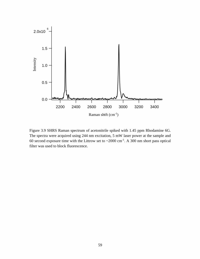
59
Figure 3.9 SHRS Raman spectrum of acetonitrile spiked with 1.45 ppm Rhodamine 6G.
The spectra were acquired using 244 nm excitation, 5 mW laser power at the sample and
60 second exposure time with the Littrow set to ~2000 cm-1. A 300 nm short pass optical
filter was used to block fluorescence.
Raman shift (cm-1)
Inte
nsi
ty
2.0x10 6
1.5
1.0
0.5
0.0
.
3400 3200 3000 2800 2600 2400 2200
.

60
Figure 3.10 UV excited fluorescence spectrum of 1.45 ppm Rhodamine 6G in acetonitrile,
measured using ocean optics spectrometer (Model: USB4000-UV-VIS) The dashed line
shows the transmission profile of the 300 nm short pass filter that was used to acquire the
UV Raman spectrum shown in Fig. 9. Other parameters include 244 nm excitation, 5 mW
laser power at sample and one second acquisition time.

61
Chapter 4
Standoff Spatial Heterodyne Raman Spectroscopy
4.1. Background
Standoff Raman spectroscopy has been defined as Raman spectroscopy performed
where the spectrometer (and therefore the operator) is some distance from the sample under
interrogation.1 The basic idea of standoff Raman spectroscopy is well illustrated in Fig.
4.1. In general, a laser is used to illuminate the sampling region, which can potentially be
at any distance from the instrument and the return light is collected by a telescope. Standoff
Raman spectroscopy is a valuable tool for remote detection and identification of chemicals
for the applications where close proximity to the target is potentially hazardous2 (e.g.,
explosives), or where remote measurement is the only option, like space applications.3 The
key features that make Raman spectroscopy an ideal tool for standoff measurements
include:1)Raman is a scattering technique, that is, there is no need for sample preparation;
a necessary condition for field-based measurements where the sample is inaccessible, 2)
Raman shifts are independent of excitation wavelength, consequently, the daylight
measurements can be accomplished using a deep UV laser in the solar blind region,4 3)
The use of a pulsed laser and fast-gated detection system allows measurements to be made
in ambient light conditions and also enables real time monitoring of samples, 4) Raman

62
measurements can also be conducted in extreme environmental conditions such as in fog 4
heavy rain,5 snow6 and at elevated temperatures7.
The basic concept of standoff Raman spectroscopy was first described in 1968.8
However, it was not until the early 1970s that instrumentation was developed to the point
that remote Raman of atmospheric gases was possible.9-12 The first truly portable, stand-
off Raman spectrometer was described in 1992 by Angel13 and his group for the
measurement of inorganic compounds such as K4[Fe(CN)6], NaNO2 and NaNO3, as well
as organic substances like CCl4 and acetaminophen, at tens of meters for analysis of
radioactive wastes in underground storage tanks. Since 1992 the number of publications
describing standoff Raman systems and applications has steadily increased with
measurements described at ranges from meters, up to 500 meters.14,15Applications of
standoff Raman include analysis of art and archeological artifacts,16 hazardous chemical
detection,2,17,18 environmental and geochemical measurements,19 and measurements in
space science3. The application of standoff Raman to geological measurements is a very
active area, pioneered by Sharma and his groups.19
4.2. Standoff Raman system and Instrumentation Overview
The essential parts of a standoff Raman system are similar to that of a traditional
Raman system, with the main component being a laser, collection optics, spectrometer,
detector, and optical filters. The major difference is the use of a telescope for collection of
scattered radiation from the remote target. The telescope is incorporated to compensate for
the diminished signal with distance. Like in conventional Raman measurements, both
pulsed and CW lasers have been used, but pulsed lasers are usually preferred for their

63
ability to be coupled with gated detectors, helpful in reducing ambient light background
during daytime measurements. Most standoff Raman systems utilize a charge-coupled
device (CCD) or intensified CCD (ICCD) detectors. ICCD detectors are most common
because they can be synchronized with the pulsed laser, allowing collection only during
the arrival time of Raman photons at the detector so that ambient light can be effectively
minimized. Additionally a pulsed laser with a gated ICCD detector offers the opportunity
of conducting time-resolved measurements, which helps to discriminate fluorescence in
luminescent minerals.21 A number of spectrometer designs have been proposed for
analyzing collected light, some of them include, dispersive, coded aperture,21 AOTF,22
among which the dispersive spectrometers are the most commonly used. A study by
Sharma et al.23 revealed that small f/# number spectrometers perform better than larger f/#
spectrometers for standoff systems.
4.3 Geometry of Collection optics
Since, the scattered radiation is collected from a distance, the sample being
illuminated with a laser must be in a line of sight of the collection optics, and a minor
misalignment could result in a huge loss in signal. Therefore, the collection optics and laser
must be properly aligned. The geometry of the laser and the telescope relative to the sample
location can be set up in two ways, coaxial and oblique (sometimes referred to as bi-axial).
Figure 2 shows a typical co-axial optical layout for standoff configuration. In a co-axial
geometry (path A in Fig 2), the sample is illuminated with the laser, which is the optical
axis of the telescope, by using small mirrors or prisms. The benefit of this configuration is
that the realignment is not necessary while changing the sample position.23 However, there
is the possibility of decrease in signal intensity due to a loss of laser power at the beam

64
steering optics. In an oblique geometry (path B in Fig. 2), the excitation laser is placed next
to the telescope, and is focused onto the target that also corresponds to the focal point of
the telescope. The primary benefit of oblique geometry is that it retains the full power of
the laser. However, the system has to be realigned if the target or sample distance
changes.23 Sharma and his research group showed that co-axial configuration offers a wider
range of sampling depth while oblique preserve the scattering signal.13
4.4 Standoff system coupling
Coupling the SHRS to the light collection optics is relatively straightforward.
However, the overall system must be designed accurately to avoid optical losses. Light
from the output of the telescope after passing through laser blocking filters can be
efficiently transferred to the spectrometer in two ways; directly using intermediate lenses
or by using fiber optic cables. The choice of method largely depends on the size of the
spectrometer and the available space. A fiber optic coupling is easy to implement, and gives
more freedom and flexibility in placing the individual components, but can lead to system
inefficiency due to the small fiber size and optical losses inside the fiber. A study by Mishra
et al. showed that a directly coupled system offers better performance over a fiber coupled
system by a factor of 10 for a system with coaxial geometry.18 However, directly coupled
systems need more space as all components have to be on the same axis and can be much
heavier than a fiber optic couple. Both types of coupling have been proven useful for
planetary measurements because of their small size, mass, and low power requirements 18

65
4.5 References
1. A.J. Hobro, B. Lendl. “Stand-off Raman spectroscopy”. TrAC Trends Anal. Chem. 2009.
28(11): 1235–1242.
2. Existing and Potential Standoff Explosives Detection Techniques. National Academies
Press, Washington, D.C., 2004.
3. S.M. Angel, N.R. Gomer, S.K. Sharma, C. McKay. “Remote Raman Spectroscopy for
Planetary Exploration: A Review”. Appl. Spectrosc. 2012. 66(2): 137–150.
4. M. Wu, M. Ray, K.H. Fung, M.W. Ruckman, D. Harder, A.J. Sedlacek. “Stand-off
Detection of Chemicals by UV Raman Spectroscopy”. Appl. Spectrosc. 2000. 54(6):
800–806.
5. A. Pettersson, S. Wallin, H. Östmark, A. Ehlerding, I. Johansson, M. Nordberg, et al.
Explosives standoff detection using Raman spectroscopy: from bulk towards trace
detection. In: R.S. Harmon, J.H. Holloway, Jr., J.T. Broach, editors. 2010. P. 76641K–
76641K–12.
6. A. Pettersson, I. Johansson, S. Wallin, M. Nordberg, H. Östmark. “Near Real-Time
Standoff Detection of Explosives in a Realistic Outdoor Environment at 55 m Distance”.
Propellants Explos. Pyrotech. 2009. 34(4): 297–306.
7. J.P. Young, S. Dai, Y. Lee, H. Xizo. Application of Raman Spectroscopy to High-
Temperature Analytical Measurements. Oak Ridge National Lab., TN (United States),
1997.
8. J. Cooney. "Satellite Observations Using Raman Component of Laser Backscatter". In:
Ralph Zirkind editor. New York: Polytechnic Institute of Brooklyn Press, 1967. Pp. P1-
P1
9. .T. Hirschfeld. “Remote spectroscopic analysis of ppm-level air pollutants by Raman
spectroscopy”. Appl. Phys. Lett. 1973. 22(1): 38.
10. J. Cooney, K. Petri, A. Salik. “Measurements of high resolution atmospheric water-
vapor profiles by use of a solar blind Raman lidar”. Appl. Opt. 1985. 24(1): 104.
11. D.A. Leonard. “Observation of Raman Scattering from the Atmosphere using a Pulsed
Nitrogen Ultraviolet Laser”. Nature. 1967. 216(5111): 142–143.
12. U.N. Singh, Z. Chu, R. Mahon, T.D. Wilkerson. “Optimization of a Raman shifted dye
laser system for DIAL applications”. Appl. Opt. 1990. 29(12): 1730.

66
13. S.M. Angel, T.J. Kulp, T.M. Vess. “Remote-Raman Spectroscopy at Intermediate
Ranges Using Low-Power cw Lasers”. Appl. Spectrosc. 1992. 46(7): 1085–1091.
14. S.K. Sharma, A.K. Misra, P.G. Lucey, S.M. Angel, C.P. McKay. “Remote Pulsed
Raman Spectroscopy of Inorganic and Organic Materials to a Radial Distance of 100
Meters”. Appl. Spectrosc. 2006. 60(8): 871–876.
15. R.L. Aggarwal, L.W. Farrar, D.L. Polla. “Measurement of the absolute Raman
scattering cross sections of sulfur and the standoff Raman detection of a 6-mm-thick
sulfur specimen at 1500 m”. J. Raman Spectrosc. 2011. 42(3): 461–464.
16. P. Vandenabeele, J. Jehli ka. “Mobile Raman spectroscopy in astrobiology research”.
Philos. Trans. R. Soc. Math. Phys. Eng. Sci. 2014. 372(2030): 20140202–20140202.
17. S. Sadate. “Standoff Raman Spectroscopy of Explosive Nitrates Using 785 nm Laser”.
Am. J. Remote Sens. 2015. 3(1):1.
18. G. Tsiminis, F. Chu, S. Warren-Smith, N. Spooner, T. Monro. “Identification and
Quantification of Explosives in Nanolitre Solution Volumes by Raman Spectroscopy in
Suspended Core Optical Fibers”. Sensors. 2013. 13(10): 13163–13177.
19. A.K. Misra, S.K. Sharma, C.H. Chio, P.G. Lucey, B. Lienert. “Pulsed remote Raman
system for daytime measurements of mineral spectra”. Spectrochim. Acta. A. Mol.
Biomol. Spectrosc. 2005. 61(10): 2281–2287.
20. A.K. Misra, S.K. Sharma, P.G. Lucey. “Remote Raman Spectroscopic Detection of
Minerals and Organics Under Illuminated Conditions from a Distance of 10 m Using a
Single 532 nm Laser Pulse”. Appl. Spectrosc. 2006. 60(2): 223–228.
21. B.J. Bozlee, A.K. Misra, S.K. Sharma, M. Ingram. “Remote Raman and fluorescence
studies of mineral samples”. Spectrochim. Acta. A. Mol. Biomol. Spectrosc. 2005.
61(10): 2342–2348.
22. E.C. Cull, M.E. Gehm, B.D. Guenther, D.J. Brady. Standoff raman spectroscopy system
for remote chemical detection. In: A.J. SedlacekIII, S.D. Christesen, R.J. Combs, T. Vo-
Dinh, editors. 2005. P. 59940H–59940H–8.
23. N. Gupta, R. Dahmani. “AOTF Raman spectrometer for remote detection of
explosives”. Spectrochim. Acta. A. Mol. Biomol. Spectrosc. 2000. 56(8): 1453–1456.

67
Figure 4.1. Typical optical system schematic for a standoff Raman spectroscopy. The
picture in bottom inset was taken from www.pict.ru.

68
Figure. 4.2. Schematic of standoff Raman system showing (A) co-axial, used for UV
excitation, and (B) oblique, used for visible excitation, geometries for laser and telescope
optical paths.

69
Chapter 5
UV Standoff Raman Measurements Using a Gated Spatial Heterodyne Raman
SpectrometerB
5.1 Abstract
A spatial heterodyne Raman spectrometer (SHRS) is evaluated for standoff Raman
measurements in ambient light conditions using both UV and visible pulsed lasers with a
gated ICCD detector. The wide acceptance angle of the SHRS simplifies optical coupling
of the spectrometer to the telescope and does not require precise laser focusing or
positioning of the laser on the sample. If the laser beam wanders or loses focus on the
sample, as long as it is in the field of view of the SHRS, the Raman signal will still be
collected. The SHRS is not overly susceptible to vibrations, and a vibration isolated optical
table was not necessary for these measurements. The system performance was assessed by
measuring standoff UV and visible Raman spectra of a wide variety of materials at instance
up to 18 m, using 266 nm and 532 nm pulsed lasers, with 12.4” and 3.8” aperture
telescopes, respectively
B N. Lamsal, S.M. Angel, S.K. Sharma, T.E. Acosta. “UV Standoff Raman Measurements
Using a Gated Spatial Heterodyne Raman Spectrometer.” Appl. Spectrosc. 2016. 70(4).
Published online ahead of print by Sage Publications Ltd. The online version of this article
can be found at http://asp.sagepub.com/content/early/2016/02/16/0003702816631304.full

70
5.2 Introduction
Raman spectroscopy is a valuable tool for chemical identification because the
relatively sharp Raman bands provide detailed molecular structural information for organic
and inorganic compounds.1 Raman is a scattering technique and no sample preparation is
required, thus Raman measurements can in principle be made for any sample within line
of sight. This is taken advantage in standoff Raman spectroscopy where samples are
measured from a distance, often desirable to minimize the risk associated with measuring
hazardous samples like explosives, and also useful for measuring inaccessible samples. In
standoff Raman spectroscopy, a laser is used to excite the sample at a distance (e.g., tens
to hundreds of meters) from which the inelastic scattered Raman photons are collected
using a large aperture optical system such as a telescope that is coupled to a Raman
spectrometer.
Standoff Raman spectroscopy was initially developed in the 1960s,2,3 and later used
primarily for the detection of atmospheric gases such as sulfur dioxide, nitrogen and
oxygen.3-5 In 1992, standoff Raman was extended by Angel et al.,6 to include the
measurement of inorganic compounds such as K4[Fe(CN)6], NaNO2 and NaNO3, as well
as organic substances like CCl4 and acetaminophen, at tens of meters using a portable
standoff Raman system that was developed for analysis of radioactive wastes in
underground storage tanks. Some recent improvements in standoff Raman systems include,
the use of gated detection for daylight operations,7,8 extreme range measurements up to
1500 m,9 systems for explosives detection8, 10-12 and planetary exploration,13-15 and deep-
UV systems which take advantage of higher Raman cross sections and resonance
enhancement in the UV.10, 16-22 UV excitation provides larger Raman cross sections and it

71
has been shown that deep-UV Raman spectra are free from interference from longer
wavelength fluorescence, which often plagues visible wavelength Raman measurements.23
Utilizing UV excitation for standoff Raman generally requires a high-resolution
spectrometer to discern the Raman signal that occurs over a very narrow spectral range.
Moreover, low laser irradiance must often be used to avoid laser-induced photodegradation
of the sample. Spectrometers that provide sufficiently high spectral resolution for deep-UV
standoff Raman typically are large and have low light throughput because of the need of
large, high dispersion gratings, and long focal length optics.
The spatial heterodyne Raman spectrometer is a compact, high resolution
instrument that has been shown to be useful in the deep-UV,24,25 and might be well suited
for standoff UV Raman measurements. The first spatial heterodyne Raman spectrometer
(SHRS) was described by Gomer et al. for visible Raman measurements,26 and extended
into the deep UV by Lamsal et al.24,25 The SHRS is based on a stationary diffraction grating,
heterodyned interferometer. As such, there is no entrance slit; light enters the spectrometer
through a large aperture, and the resolution of the spectrometer is not a strong function of
the aperture size. Heterodyning in the interferometer allows high spectral resolution to be
achieved with a relatively small number of samples, fixed by the number of horizontal
pixels on the imaging detector. The large entrance aperture and wide acceptance angle of
the SHRS provides high light throughput and allows large laser spots to be used on the
sample without light loss or the loss of spectral resolution.
In the case of standoff Raman, this also makes the SHRS relatively easy to couple
with telescopic optics and minimizes laser pointing stability issues, because small

72
movements of the laser spot on the target do not reduce the amount of light collected by
the spectrometer slit, unlike the case of a dispersive spectrometer where the output of the
telescope has to be held in focus on a narrow input slit. In addition, all wavelengths are
measured simultaneously in the SHRS, making it compatible with pulsed lasers and gated
detection, which has been shown to be useful for making Raman measurements in
daylight.8 The SHRS is also not overly susceptible to vibrations and does not necessarily
require a vibration isolation system. These characteristics make the SHRS especially
suitable for UV standoff Raman measurements. In this work, we present standoff Raman
spectra of several types of samples located up to 18 m from the spectrometer, using 266
and 532 nm pulsed laser excitation in bright light conditions, and without the use of a
vibration isolation system.
5.3 Experimental
A schematic of the standoff SHRS instrument for Raman measurements is shown
in Fig. 1.1 The system consists of three components; the excitation source, the light
collection optics and the SHRS spectrometer.
5.3.1 The excitation source
Q-switched Nd:YAG lasers were used to generate 532 nm (Quantel, Ultra CFR)
and 266 nm (Quantel, Brilliant Eazy) laser pulses of pulse width 6 ns and 4 ns, respectively.
The visible laser was operated at 20 Hz using 5.3 mJ/pulse, and the sample was illuminated
at an angle of about 30° relative to the optical axis of the telescope (path b in Fig. 1). Note:
180° backscatter would have been preferred for this measurement but the proper mirrors
were not available at the time of this study. The UV laser was operated at 10 Hz using 10.3

73
mJ/pulse, and the beam was collinear with the telescope optical axis. A beam expander was
used to defocus the beam, creating large laser spots on the sample from ~7 mm for the
closest samples, to ~25 mm for the samples at 20 m (path a in Fig. 1), to avoid laser-induced
photodecomposition and sample heating. The average laser power was monitored using a
power meter. In some cases laser pulse energy is provided, calculated form the average
power measurement and the known laser pulse frequency.
5.3.2 Collection optics
For 532 nm standoff measurements, an f/16, 3.8-inch aperture telescope (Questar
FR-1 MK III) with a collimated beam output was used for light collection. Light collected
by the telescope was directly coupled to the SHRS, with laser rejection and spectral
bandpass filters placed in the collimated beam before the SHRS entrance aperture. For 266
nm standoff measurements, an f/9.1, 12.4-inch aperture custom-made Ritchey Chretien
telescope (Optical Guidance Systems, Model RC12.5), with UV optics was used for light
collection. Light collected by the telescope was collimated using an anti-reflection coated,
1-inch diameter, f/12, fused silica lens, and guided to the SHRS by two flat aluminum
coated mirrors.
5.3.3 SHRS spectrometer
The SHRS interferometer, shown in more detail schematically in Fig. 2, consists of
a 20 mm fused silica cube beam splitter (Esco Optics, Model O420120, λ/10 Beamsplitter
Cube) and a pair of 300 grooves/mm, 25 mm square diffraction gratings blazed at 300 nm.
Two 532 nm or 266 nm laser-blocking filters were employed (Semrock RazorEdge, LP03-
532RE-25 and LP02-266RS-25, respectively) before the entrance of the SHRS. In addition,

74
short-pass filters for UV (Semrock BrightLine, FF01-300/SP-25) or band-pass filters for
visible (Semrock BrightLine, FF01-558/20-25) were used to block longer wavelengths.
The gratings were mounted in piezo motor driven optical mounts connected with a piezo
motor controller (Newport, Model AG-UC8) and positioned on a precision rotation stage
(Newport, Model URS75BPP) for setting the Littrow angle precisely to the desired
wavelength. The interference fringe pattern was produced by imaging the gratings onto a
thermo-electrically cooled, gated, 25 mm wide by 6.7 mm high, 1024 by 256 ICCD array
detector, (Princeton Instruments, Model PIMAX 3), using a 105 mm focal length, f/4 fused
silica lens (JENOPTIK CoastalOpt® 105 mm UV-Vis SLR lens). The imaging lens was
placed approximately 245 mm from the gratings and ~185 mm from the detector to form a
15 mm square fringe image on the ICCD detector, with substantial clipping in the vertical
direction. The ICCD gate width and delay time were adjusted at each measurement distance
to maximize the Raman signal and reduce ambient light.
For most spectra three additional images were acquired for background corrections;
two blocking each of the gratings separately and one blocking both gratings. The Fourier
transform of the fringe images was performed using the Fast Fourier transform (FFT)
function in Matlab. Each spectrum was apodized using a Hamming function to reduce
ringing effects in the spectral baseline, though no studies were done to determine if this
apodiztaion function was optimal. No flat field or instrument response corrections,
smoothing, sharpening, or any other post-processing was used.

75
5.4 Result and Discussions
The working principle of the SHRS has been described in earlier papers.24-26 As
illustrated in Fig. 2, collected light is collimated and directed through the SHRS entrance
aperture. A 50/50 beamsplitter divides the light into two coherent beams, directed to the
diffraction gratings that are tilted at an angle, the Littrow angle ƟL, with respect to the
grating normal. Heterodyning in the interferometer occurs at the Littrow wavenumber, ƟL,
which corresponds to the wavelength of light that is exactly retro-reflected, back along the
optical axis, and hence recombines at the beamsplitter without interference. For any
wavenumber () other than Littrow, the diffracted light leaves the gratings at an angle,
resulting in crossed wavefronts in the beamsplitter, generating an interference pattern,
which produces a series of wavelength dependent fringes on the array detector. The fringe
frequency on the detector is given by Eq. 1, where f is in fringes/cm.24, 27-29 According to
Eq. 1, Raman bands above or below the Littrow wavenumber show identical fringe patterns
and can lead to degenerate Raman bands. This is discussed in more detail below. The
intensity, I(x), of fringes obtained as a function of detector position, x, is given by Eq. 2,
where B() is the input spectral intensity at wavenumber σ. The Fourier transform of I(x)
yields the Raman spectrum.24, 27-29
𝑓 = 4 (σ − σL) tanθL (1)
𝐼(𝑥) = ∫ 𝐵(σ)[1 + cos8π(σ − σL) 𝑥 tan θL]
∞
0
𝑑σ (2)
Like all interferometers, it is important to block all wavelengths outside the spectral
regions of interest. Shot noise is distributed equally at all wavelengths in an interferometer,

76
so strong bands outside the spectral region of interest add noise at all wavelengths. Of
particular concern is scattered laser light and strong fluorescence. Thus, the use of optical
filters to limit the bandpass of the spectrometer is crucial in the SHRS. To prevent
elastically scattered laser light entering the spectrometer two 532 nm or 266 nm laser-
blocking filters (RazorEdge, Semrock) were employed before the entrance of the SHRS.
In addition, short-pass or band-pass optical filters were used to block longer wavelengths.
The theoretical spectral bandpass of the SHRS is a function of the resolving power
and the number of detector elements on the ICCD in the spectral direction. The resolving
power is equal to the number of grooves illuminated, so in this case R=12,000, giving a
theoretical resolution of ~3 cm-1 for a 1000 cm-1 Raman shift, using 266 nm excitation and
~1.5 cm-1 using 532 nm excitation. The measured UV spectral resolution was previously
determined to be 4.5 cm-1 using a diamond sample.24 Factors that affect the resolution
include camera focusing, collimation of input beam, and quality of the gratings and
imaging optics, with grating imperfections appearing to be the most important in our
current setup. The ICCD used had 1024 spectral resolution elements and can thus be used
to measure 512 wavelength elements, giving a theoretical ICCD-limited UV spectral range
of ~1600 cm-1. The maximum, resolution-limited solid angle field of view (FOV) of the
SHRS is, Ωmax = 2π/R steradian.27 Thus the solid angle FOV for this spectrometer is 5.2 x
10-4 sr, and the full acceptance angle is 1.3°.
Although UV excitation offers potential sensitivity advantages for standoff Raman,
UV excitation is difficult to implement because strong sample absorption in the UV often
leads to photodecomposition of the sample. For example, in these UV standoff studies, it
was found that using the 266 nm laser, calcite was damaged by 23 mJ pulses but was not

77
affected using 10 mJ pulses. Acetaminophen on the other hand was damaged at all laser
energies tested. Lowering the laser power is effective at reducing sample decomposition;
however, it also has the effect of reducing Raman signal. An alternative approach is to
reduce the laser irradiance on the sample while keeping the laser power high, by increasing
the size of the laser spot on the sample. In this case, the Raman signal is not reduced as
long as the field of view of the spectrometer is at least as large as the laser spot on the
sample. We demonstrated this in a previously published study by measuring a
photosensitive compound, NH4NO3, using the SHRS with 244 nm excitation with a large
laser spot on the sample.24 Thus, in this standoff study, using 266 nm excitation, to avoid
sample decomposition, the largest possible laser spot that could be viewed by the SHRS
was used. As shown above, the full acceptance angle of the UV SHRS was ~1.3o. The
magnification of the telescope at 18 m was about 5.3, corresponding to a ~37 mm diameter
spot on the sample at 18 m standoff distance (note: the telescope at this range was
effectively f/11). The laser spot size for all UV standoff Raman measurements was about
25 mm diameter, well within the FOV of the standoff spectrometer. It is interesting to
compare the SHRS FOV to a hypothetical dispersive standoff spectrometer. The slit image
of an f/6.7 dispersive spectrometer using a 100-micron wide input slit, f/# matched to the
same telescope would be ~0.9 mm wide at 18 m, and the total area viewed at the sample
would be ~1800 times smaller, assuming a circular field of view in each case, limited by
the shape of the focused laser beam.
5.4.1 UV Wavelength Standoff Raman Measurements
Figure 3 shows standoff SHRS UV Raman spectra of several samples that were
placed at a distance of 18 m from the telescope. The samples, KClO3 (a), urea (b), calcite

78
(c), and KClO4 (d), were measured using 600, 10.3 mJ laser pulses (i.e., 60 s exposure
time) with all laboratory lights on and using a 0.18 s gate delay and 0.05 s gate width.
The SHRS was tuned to cover the spectral range 600-2000 cm-1 (by setting Littrow at ~600
cm-1) because this range contains the key spectral features of these samples. The prominent
Raman bands of KClO3 at 937 cm-1 (ClO3- vibrational mode), urea at 1013 cm-1 (C-N
vibrational mode), calcite at 1087 cm-1 (CO3- vibrational mode), and KClO4 at 942 cm-1
(ClO4- vibrational mode), are clearly observed, free from any background ambient light,
with a measured spectral resolution of ~10 cm-1.
Figure 4 shows the standoff SHRS UV Raman spectrum of Teflon with the sample
18 meters from the telescope using 600, 10.3 mJ, 266 nm pulses (i.e., 60 s exposure time).
Littrow was set to ~495 cm-1 and all lab lights were on. The gate delay and gate width were
0.18 s and 0.05 s, respectively. The fringe image (top inset) and fringe image cross
section (middle inset) are also shown in Fig. 4. The fringe visibility (FV) value is ~0.32,
much less than the 1.0 theoretical value for monochromatic light. The reason for the low
FV is poor UV transmission and optical imperfections in the beam splitter. Poor fringe
visibility leads to increased noise in the SHRS spectra and is one of the current limitations
of the UV SHRS. A possible improvement to this part of the system would be to use a plate
beam splitter, since plate beam splitters are available with much better UV transmission
and surface flatness than cube beam splitters.
The SHRS Teflon spectrum in Fig. 4 displays several characteristic Raman bands
with no significant ambient light background. The sharp Raman band of Teflon at 734 cm-
1 corresponds to the F-C-F stretching mode, and the 1200-1400 cm-1 spectral region shows
bands for the F-C-F anti-symmetric stretching mode (1215 cm-1) and C-C vibrational

79
modes (~1296 cm-1 and ~1378 cm-1). The measured resolution of this band was 11 cm-1,
much larger than the ~4.5 cm-1 spectral resolution of the SHRS as verified previously using
a diamond sample.24 For this measurement, the input beam was focused slightly so that
more light hit the small ICCD (e.g., was less clipped vertically), leading to reduced
resolution but higher sensitivity.
The Raman bands at ~ 576 cm-1 are related to crystal defect structures.30 The
position of the Raman bands and the relative intensities shown in Fig. 4 are in qualitative
agreement with published data,16,31 even though no correction was made for the instrument
response function. The two bands at ~611 and ~693 cm-1 are likely the 291 cm-1 (F-C-F
twisting) and 387 cm-1 (F-C-F bending) Teflon bands, respectively. As shown by Eq. 1,
there is no discrimination between bands that are higher or lower than the Litrrow
wavenumber. Heterodyning of Raman bands below the Littrow wavenumber can lead to
low energy bands being shifted to higher energy spectral regions. This effect can be useful
for extending the spectral range of the SHRS, or this degeneracy can be completely avoided
by tilting one of the gratings in the vertical direction.26
5.4.2 Visible Wavelength Standoff Raman Measurements
Visible wavelength standoff SHRS measurements were made by simply adjusting
the Littrow angle of the gratings to the visible wavelength range. Figure 5 shows the
standoff Raman spectra of NH4NO3, TiO2, and sulfur, acquired using the SHRS with a 532
nm, 20 Hz pulse rate laser, and a 96 mm aperture telescope. The spectra were recorded
from various standoff distances in the range 3 to 14 m with the laser power from 60-106

80
mW using a 60 s exposure time. The laser spot size at the sample varied from 7 mm for the
closest samples to 25 mm for the most distant samples.
Fig. 5(a) shows the Raman spectrum of NH4NO3 at a sample distance of 3 m using
62 mW laser power with a 7 mm laser spot size on the sample. Using a 7 mm laser spot,
no sample decomposition was observed. The spectrum was obtained using the SHRS with
a Littrow wavelength of 550 nm (700 cm-1 Raman shift from the laser line) and using a 558
nm band pass filter to block lower frequency Raman signals. Ammonium nitrate is widely
used as a precursor for explosives manufacture. Therefore, remote measurements of
ammonium nitrate could be useful for explosives detection. The SHRS spectrum of
ammonium nitrate shows a strong Raman band at 1040 cm-1 due to the NO3- symmetric
stretching mode, the FWHM of which was 5.4 cm-1. Figure 5(b) shows the Raman spectrum
of TiO2 measured with the sample 10 m from the telescope, using 103 mW laser power at
the sample with the Littrow wavelength set to the laser wavelength (0 cm-1 Raman shift).
The laser spot size on the sample was ~20 mm, much smaller than the >45 mm field of
view (0.27o FOV) of the SHRS at this distance, calculated assuming a collimated beam.
The Raman spectrum of sulfur shown in Fig. 5(c) was measured with the sample at a
standoff distance of 14 m using 106 mW laser power with Littrow set to 532 nm and using
a 25 mm laser spot on the sample. Figure 5(c) also shows the sulfur fringe image (inset
top) and the fringe image cross section (inset middle). The FV value of the fringe cross
section is only 0.22, much less than the theoretical value of 1.0 for monochromatic light.
The low FV value in this case is because the UV beamsplitter used had poor visible
wavelength transmission. The main sulfur Raman bands in the spectrum are at 85 cm-1, 154
cm-1, 219 and 473 cm-1. The relative intensity of the Raman band at 473 cm-1 is lower than

81
the band at 85 cm-1 because of the decreasing response of SHRS in the higher frequency
region.
5.4.3 UV Stability Study
An interferometer is susceptible to changes in the optical path length in the arms,
usually caused by vibrations, and for this reason, interferometer-based spectrometers are
commonly used on a vibration-isolation table. In the standoff SHRS studies described here,
it was found that the SHRS was not highly susceptible to vibrational misalignment. Fig. 6
shows Raman spectra of diamond, which has a very sharp band at ~1333 cm-1, measured
using a 244 nm continuous wave laser, with and without vibration isolation (i.e., using a
floating and non-floating optical table). The FV was 0.36 for all spectra. Also, the spectral
position of the band and the FWHM are unchanged using short, 0.5 s, and long, 60 s
exposures with or without vibration isolation, indicating no effect of system vibrations on
the Raman spectrum over this measurement time. Figure 7 shows the results of a similar
test using the standoff SHRS. The bandwidth and position of sulfur bands were measured
using short, 1s, and long, 60s, exposures with the laser on a lab bench that was not vibration
isolated. Figure 7 shows Raman spectra of sulfur measured by integrating 20 (1 s), 600 (30
s) and 1200 (60 s) laser pulses, respectively with the sample at a 10 meter standoff distance.
The fringe visibility was the same, 0.25, and the FWHM of the 154 and 219 cm-1 bands
was 10-11 cm-1, for all three exposures. The band positions were also the same within one
pixel. This indicates vibrational stability of the standoff SHRS at this time scale.

82
5.5 Conclusions
The spatial heterodyne Raman spectrometer is well suited for both UV and visible
standoff Raman measurements. The large aperture and wide acceptance angle of the SHRS
simplifies optical coupling of the spectrometer to the telescope, and makes alignment of
the laser on the sample very forgiving. The use of a pulsed laser and a gated detector allows
SHRS measurements to be made in bright ambient light. The SHRS is sufficiently
unaffected by system vibrations for the exposure times used, that a vibration isolated
optical table was not necessary for the measurements described. Although signal to noise
comparisons between the SHRS and dispersive Raman systems for standoff Raman were
not part of this study, this was addressed recently in regard to FT Raman spectrometers.32
5.6 Acknowledgements
We would like to thank the National Science Foundation for supporting this work
under grant CHE-1308211 and NASA for support under grant NNX14AI34G and
NASA/SC Space Grant 21-NE-USC_Angel-RGP. We also thank the Research Corporation
of the University of Hawaii (RCUH) /NAVSEA/DOD, for partial support of this work
under contract number. ZA01339. This work has also benefited in part by the support from
the Office of Naval Research under the grant #N00014-12-1-0087.

83
5.7 References
1. J.R. Ferraro, K. Nakamoto, C.W. Brown. “Industrial, Environmental and Other
Applications”. In: F. K. Nakamoto C. W. Brown, editors. “Introductory Raman
Spectroscopy”. San Diego: Academic Press, 2003. Pp. 325–361.
2. J. Cooney. "Satellite Observations Using Raman Component of Laser Backscatter". In:
Ralph Zirkind editor. New York: Polytechnic Institute of Brooklyn Press, 1967. Pp.
P1- P10.
3. D.A. Leonard. “Observation of Raman Scattering from the Atmosphere using a Pulsed
Nitrogen Ultraviolet Laser”. Nature. 1967. 216(5111): 142–143.
4. T. Hirschfeld. “Range Independence of Signal in Variable Focus Remote Raman
Spectrometry”. Appl. Opt. 1974. 13(6): 1435-1437.
5. R.M. Measures. Laser Remote Sensing: Fundamentals and Applications. New York:
John Wiley & Sons, 1984.
6. S.M. Angel, T.J. Kulp, T.M. Vess. “Remote-Raman Spectroscopy at Intermediate
Ranges Using Low-Power CW Lasers”. Appl. Spectrosc. 1992. 46(7): 1085–1091.
7. J.C. Carter, J. Scaffidi, S. Burnett, B. Vasser, S.K. Sharma, S.M. Angel. “Stand-off
Raman Detection using Dispersive and Tunable Filter Based Systems”. Spectrochim.
Acta. A. Mol. Biomol. Spectrosc. 2005. 61(10): 2288–2298.
8. J.C. Carter, S.M. Angel, M. Lawrence-Snyder, J. Scaffidi, R.E. Whipple, J.G.
Reynolds. “Standoff Detection of High Explosive Materials at 50 Meters in Ambient
Light Conditions Using a Small Raman Instrument”. Appl. Spectrosc. 2005. 59(6):
769–775.
9. R.L. Aggarwal, L.W. Farrar, D.L. Polla. “Measurement of the Absolute Raman
Scattering Cross Sections of Sulfur and the Standoff Raman Detection of a 6 mm thick
Sulfur Specimen at 1500 m”. J. Raman Spectrosc. 2011. 42(3): 461–464.
10. M. Gaft, L. Nagli. “UV Gated Raman Spectroscopy for Standoff Detection of
Explosives”. Opt. Mater. 2008. 30(11): 1739–1746. doi:10.1016/j.optmat.2007.11.013.
11. J. Moros, J.A. Lorenzo, K. Novotný, J.J. Laserna. “Fundamentals of Stand-off Raman
Scattering Spectroscopy for Explosive Fingerprinting”. J. Raman Spectrosc. 2013.
44(1): 121–130.
12. A. Pettersson, S. Wallin, H. Östmark, A. Ehlerding, I. Johansson, M. Nordberg, H.
Ellis, A. Al-Khalili. “Explosives Standoff Detection using Raman spectroscopy: From
Bulk Towards Trace Detection”.Proc. SCIE. 2010.76641K: 1–12.

84
13. P.G. Lucey, T.F. Cooney, S.K. Sharma. “A Remote Raman Analysis System for
Planetary Landers”. Paper presented at LPSC. 1998. Houston TX; March 16-20 1998.
14. Horton, K. A., N. Domergue-Schmidt, S. K. Sharma, P. Deb, and P. G. Lucey. “Remote
Raman System for Planetary Landers: Data Reduction and Analysis”. Paper presented
at LPSC. 200. Houston TX; March 13-17 2000.
15. S.M. Angel, N.R. Gomer, S.K. Sharma, C. McKay. “Remote Raman Spectroscopy for
Planetary Exploration: A Review”. Appl. Spectrosc. 2012. 66(2): 137–150. 10.
16. M. Wu, M. Ray, K.H. Fung, M.W. Ruckman, D. Harder, A.J. Sedlacek. “Stand-off
Detection of Chemicals by UV Raman Spectroscopy”. Appl. Spectrosc. 2000. 54(6):
800-806.
17. M.D. Ray, A.J. Sedlacek, M. Wu. “Ultraviolet Mini-Raman Lidar for Stand-off, In Situ
Identification of Chemical Surface Contaminants”. Rev. Sci. Instrum. 2000. 71(9):
3485–3489.
18. M. Skulinova, C. Lefebvre, P. Sobron, E. Eshelman, M. Daly, J.-F. Gravel, J. F.
Cormier, F.Châteauneuf, G. Slater, W. Zheng, A. Koujelev, R. Léveillé. “Time-
resolved Stand-off UV-Raman Spectroscopy for Planetary Exploration”. Planet. Space
Sci. 2014. 92: 88–100.
19. T.J. Kulp, S.E. Bisson, T.A. Reichardt. “Standoff Ultraviolet Raman Scattering
Detection of Trace Levels of Explosives”. Sandia Natl. Lab. [Tech. Rep.] SAND.
2011.7955.
20. R.L. McCreery. “Magnitude of Raman Scattering”. In: T.D. Winefordner editor.
Raman Spectroscopy for Chemical Analysis. New York: John Wiley & Sons, Inc.,
2000. Pp.15-33.
21. S.A. Asher. “UV Resonance Raman Spectroscopy for Analytical, Physical, and
Biophysical Chemistry. Part 1”. Anal. Chem. 1993. 65(2): 59A–66A.
22. M. Ghosh, L. Wang, S.A. Asher. “Deep-Ultraviolet Resonance Raman Excitation
Profiles of NH4NO3, PETN, TNT, HMX, and RDX”. Appl. Spectrosc. 2012. 66(9):
1013-1021.
23. S.A. Asher, C.R. Johnson. “Raman Spectroscopy of a Coal Liquid Shows that
Fluorescence Interference is Minimized with Ultraviolet Excitation”. Science. 1984.
225(4659): 311–313.
24. N. Lamsal, S.M. Angel. “Deep-Ultraviolet Raman Measurements Using a Spatial
Heterodyne Raman Spectrometer (SHRS)”. Appl. Spectrosc. 2015. 69(5): 525–534.

85
25. N. Lamsal, S.M. Angel, S.K. Sharma, T.E. Acosta. “Visible and UV Standoff Raman
Measurements in Ambient Light Conditions Using a Gated Spatial Heterodyne Raman
Spectrometer”. Paper presented at: LPSC 2015. Woodland TX, March 16-20.2015.
26. N.R. Gomer, C.M. Gordon, P. Lucey, S.K. Sharma, J.C. Carter, S.M. Angel. “Raman
Spectroscopy Using a Spatial Heterodyne Spectrometer: Proof of Concept”. Appl
Spectrosc. 2011. 65(8): 849–857.
27. J..M. Harlander. Spatial Heterodyne Spectroscopy: Interferometric Performance at any
Wavelength Without Scanning. [Ph.D. Thesis]. Madison, Wisconsin: The University
of Wisconsin, 1991.
28. J.M. Harlander, F.L. Roesler, S. Chakrabarti. ‘‘Spatial HeterodyneSpectroscopy: A
Novel Interferometric Technique for the FUV’’. In: O.H.W. Siegmund, H.S. Hudson,
editors. EUV, X-Ray, and Gamma-Ray Instrumentation for Astronomy. Proc. SPIE.
1990. 1344: 120-131.
29. J. Harlander, R. Reynolds, F. Roesler. “Spatial Heterodyne Spectroscopy for the
Exploration of Diffuse Interstellar Emission-Lines at Far-Ultraviolet Wavelengths”.
Astrophys. J. 1992. 396(2): 730–740.
30. D.I Bowers W. F. Maddams. “The Characterization of Polymers”. The Vibrational
Spectroscopy of Polymers. Cambridge, UK: University Press, Cambridge, 1989. Pp.
185-190.
31. A.J. Sedlacek III, S.D. Christesen, T. Chyba, P. Ponsardin. ‘‘Application of UV-Raman
Spectroscopy to the Detection of Chemical and Biological Threats’’. In: A.J. Sedlacek,
R. Colton, T. Vo-Dinh, editors. Chemical and d Biological Point Sensors for Homeland
Defense. Proc. SPIE. 2004. 5269: 23-33.
32. S. Dzsaber, M. Negyedi, B. Bernáth, B. Gyüre, T. Fehér, C. Kramberger, T.
Pichlerband F. Simona, “A Fourier Transform Raman Spectrometer With Visible Laser
Excitation,” J. Raman Spectrosc. 201 (5). 46: 327–332.

86
Figure 5.1. Schematic of standoff Raman system showing (a) co-axial and (b) oblique
geometries for laser and telescope optical paths. The co-axial geometry was used for UV
excitation and oblique geometry was used for visible excitation.

87
Figure 5.2 Detailed schematic showing the layout and illustrating the working principle of
the SHRS. S= light source, CL= collection lens, E= entrance aperture, IW= input
wavefront, BS= beamsplitter, G= diffraction grating, CW= crossed wavefront, IL=imaging
lens, θL= Littrow angle.

88
Figure 5.3. UV standoff Raman spectra of (a) potassium chlorate, KClO3 (b) urea (c) calcite
(d) potassium perchlorate, KClO4 at ~18 m, measured using the SHRS spectrometer with
Littrow set to ~600 cm-1. The arrows above each spectrum refer to the appropriate intensity
axis for that spectrum. Spectra were measured using 10.3 mJ/pulse, 10 Hz pulse rate, 266
nm excitation laser and a total integration time of 60 s. Spectra are offset vertically for
clarity
7x10 6
6
5
4
3
2
2000 1800 1600 1400 1200 1000 800
20x10 6
15
10
5
0
Inte
nsi
ty
Raman shift (cm-1
)
Inte
nsi
ty
Inte
nsi
t
y
(a)
(c)
(d)
(b)

89
Figure 5.4. Teflon interferogram fringe image (top inset), intensity cross-section (middle
inset) and Raman spectrum at ~18 m, obtained using the SHRS with Littrow set to ~500
cm-1. The spectrum was measured using 10.3 mJ/pulse, 10 Hz pulse rate, 266 nm excitation
laser and a total integration time of 60 s.

90
Figure 5.5. Visible standoff Raman spectra of (a) NH4NO3, (b) TiO2 and (c) sulfur at 3, 10
and 14 m, respectively.The spectra were measured using 532 nm pulsed laser with 62, 103
and 106 mW laser power respectively and 60 s integration time. Littrow was different in
each case. The inset shows the fringe image and cross section of sulfur. Spectra are offset
vertically for clarity. The arrows above each spectrum refer to the appropriate intensity axis
for that spectrum.

91
Figure 5.6 SHRS Raman spectra of diamond measured in triplicate, using 16 mW, 244 nm
CW laser with 0.5 s and 60 s exposure times, with SHRS mounted on floating (F) and non-
floating (NF) optical table. Twelve total spectra are shown in this plot. The triplicate
measurements overlap to the extent that they cannot be discerned, indicating vibrational
stability in the SHRS during the time required to make the measurements.

92
Figure 5.7 SHRS Raman spectra of sulfur at 10 m standoff distance recorded using 20, 60
and 1200, 532 nm laser pulses, 5.3 mJ/pulse and 20 Hz pulse rate with 9.6 cm diameter
collection optics.

93
Chapter 6
Performance Assessment of a Plate Beamsplitter for Deep-UV Raman
Measurements with a Spatial Heterodyne Raman SpectrometerC
6.1 Abstract
In earlier works, we demonstrated a high resolution Spatial Heterodyne Raman
Spectrometer (SHRS) for deep UV Raman measurements, and showed its ability to
measure UV light sensitive compounds using a large laser spot size. We recently modified
the SHRS by replacing the cube beamsplitter with a custom-built plate beamsplitter with
higher light transmission, higher surface flatness and better refractive index homogeneity
than the cube beamsplitter. UV Raman measurements were performed using the modified
SHRS and compared to the previous setup. The Raman spectra obtained using the modified
SHRS exhibits much higher signal to noise ratio and show fewer spectral artifacts. In this
paper, we discuss the new spectrometer design features, the advantages over previous
designs and, and discusses some general SHRS issues such as spectral bandwidth, signal
to noise ratio characteristics and optical efficiency.
C N. Lamsal, S. M. Angel. “Performance Assessment of a Plate Beamsplitter for Deep-UV
Raman Measurements with a Spatial Heterodyne Raman Spectrometer”. Appl. Spectrosc.,
to be submitted, March.2016.

94
6.2 Introduction
Recently, we developed a new type of Fourier transform (FT) Raman spectrometer;
the spatial heterodyne Raman spectrometer (SHRS)1,2 which addresses many of the issues
related to conventional UV Raman spectrometers for planetary and other applications in
extreme environments. The SHRS uses an interferometer with stationary diffraction
gratings that utilizes a two-dimensional array detector such as a CCD or ICCD to record
the interferogram, the design of which was first introduced by Harlander3,4 for astronomical
remote sensing measurements; later modified by Gomer et al for Raman measurements.5
The SHRS system is small and lightweight, contains no moving parts, and offers the high
resolution and wide spectral range needed for deep-UV Raman measurements.
Additionally, the absence of entrance slit and the large field of view relieves the necessity
to focus the energetic laser onto a sample, thus helps to avoid sample damage. The SHRS
is compatible with pulsed lasers and gated detectors allowing the standoff measurements
in ambient light conditions. All these characteristics together make the SHRS potentially
suitable for planetary exploration such as for Mars missions.
In recent study, we demonstrated the potential of SHRS for deep-UV Raman
measurements by collecting the Raman spectra of several solid and liquid samples using
SHRS with 4.5 cm-1 resolution and ~2600 cm-1 bandpass, using a 244 nm excitation laser.1
We also showed the importance of the wide acceptance angle in reducing the laser induced
damage with defocused laser.1,2 However, the design was not optimal because of likely due
to poor optical efficiency, and low fringe visibility caused by the imperfections in the
optical components especially the beamsplitter.

95
In this paper, we report an improved UV SHRS that uses cube beamsplitter by a
narrow-band, high-grade plate beamsplitter specifically designed for UV applications. The
plate beamsplitter addresses two major issues with the previously described UV SHRS,
high optical losses and poor fringe visibility. In this paper, we discuss the performance of
the modified UV SHRS with regard to fringe visibility, SNR and instrument response and
issues with the SHRS design and instrument response.
6.3 Experimental
A schematic of the SHRS for UV Raman measurements is shown in Fig. 1. The
spectrometer design follows the one described in previous studies,1,2 but modified for deep-
UV applications by including a high precision plate beamsplitter, designed to operate in
the UV range. The SHRS interferometer consists of a pair of one inch, 300 grooves/mm
square diffraction gratings blazed for 300 nm, and a 6.25 mm thick, 25.4 mm fused silica
plate beamsplitter with Reflectance/Transmission ratio (R/T) of 50/50 (+5) in the range
240-300 nm. A compensator plate with exactly the same material and same dimension as
that of the beamsplitter was introduced in the arm reflection in order to equalize the path
length for each arms of the interferometer. The front and back surfaces of both the
beamsplitter and the compensator are vacuum UV polished with a scratch/dig specification
of 10/05. The transmitted wavefront error through each optic is less than λ/10 in the 240-
300 nm range or λ/25 at 633 nm, and each optic is provided with a broadband antireflection
coating. The gratings were mounted in piezo motor-driven optical mounts (Newport Model
AGUC8) with a piezo motor controller and positioned on a precision rotation stepper
(Newport URS75BPP Model) for setting the angle precisely to the desired Littrow
wavelength. The diffraction gratings were imaged onto a thermo-electrically cooled back-

96
illuminated UV-enhanced 2048×512, 13.5 m pixels charge-coupled detector (CCD)
(Princeton Instruments, Model PIXIS-2048 2KBUV;) using a 105 mm focal length, f/4.5
fused silica achromatic camera lens (JENOPTIK CoastalOpt 105 mm UV visible [Vis]
single-lens reflex [SLR] lens;). The imaging lens (IL in Fig. 1) was placed approximately
210 mm (~2 focal lengths) from the gratings and 210 mm from the detector, magnification~
1, to form a the interferogram image on the 6.9 mm high CCD. After recording an
interferogram, the interferogram image on the CCD is binned to produce a single-channel
interferogram cross section for each of the 2048 columns of pixels, which is then Fourier
transformed to recover the power (i.e., intensity) spectrum.
A CW 244 nm intracavity frequency-doubled Ar-ion laser (95 SHG model; Lexel),
was used for excitation with an average power up to 15 mw on the sample. The laser beam
was directed onto the sample using two 45o laser line dielectric mirrors with reflectivity
higher than 98% over the 244–257 nm range, to clean up the 244 nm line from the 488 nm
fundamental laser line. The laser was focused onto the sample using a 75 mm focal-length
quartz lens mounted on a translational microstage to allow changing the size of the laser
spot on the sample. Liquid samples were placed in a 1 cm quartz cuvette, centered on the
focus of both the collection lens and the laser focus. Solid samples, either ground and
packed in quartz cuvettes or pressed into pellets, were illuminated in the same way but
were mounted on an x,y stage for front-surface illumination. Scattered light from the
sample was collected using either a 50 mm or 75 mm focal length AR-coated quartz lens,
with the laser incident on the sample at 150o with respect to the optical axis of the collection
lens. To help reduce fluorescence, collimated light was guided into the interferometer by
two high performance dielectric mirrors placed in a 90o arrangement. These mirrors have

97
reflectivity over 95% in the wavelength range 244-266 nm, which is equivalent to a Raman
range of 0-3400 cm-1 using 244 nm excitation. In order to avoid overfilling of light on the
25.4 mm beamsplitter tilted at 45°, the input beam size was reduced to 13 mm by using
several irises in the beam path before entering into the spectrometer. A long pass filter
(Semrock, 229/244 nm stopline dual-notch filter) with OD >4 (at 244 nm) was used to
block scattered laser light.
The interferometer Littrow wavelength (i.e., grating angles) was set using either the
laser line, narrow lines from a low-pressure mercury lamp, or a narrow Raman band. CCD
fringe images were recorded using Princeton Instruments Light Field software provided
with the detector. Apart from the fringe image, three other images were acquired for each
spectrum; two by blocking each of the gratings separately and one by blocking both
gratings simultaneously. These additional images were sometimes used for background
corrections of the fringe images. Fourier transforms of the fringe images were performed
using the fast Fourier transform (FFT) function in Matlab. Each spectrum was apodized
using a Hamming function to reduce ringing effects in the spectral baseline. We examined
several other apodizing functions including Hanning, Gaussian, Blackman and Blackman-
Harris, but found the Hamming function to be best for retaining the resolution and SNR of
the recovered spectrum. The Raman spectra were calibrated by locating the position of
known Raman bands and using a polynomial fit. No flat field or instrument efficiency
corrections, phase correction, smoothing, sharpening, or any other post-processing such as
zero filling was used for any of the data presented in this paper.
98
6.4 Results and Discussions
6.4.1 Working Principle of the SHRS
During SHRS measurements, the scattered Raman light is collected, collimated and
passed through the entrance aperture and divided into two coherent beams by the 50/50
fused silica plate beamsplitter. The two beams are then diffracted by the diffraction gratings
at an angle that depends on the wavelength as:
𝑛 𝜆 = 𝑑(𝑠𝑖𝑛𝛼 + 𝑠𝑖𝑛𝛽) (1)
Where n is diffraction order, λ is the wavelength of interest, d is diffraction grating groove
density, and α and β are the angles of incidence and diffraction. Heterodyning in the
interferometer is achieved by setting the grating angles in such a way that the light at
wavelength (λL) or wavenumber (σL) is exactly retroreflected back along the same beam
path. For 1st order diffraction,
Ɵ𝐿 = 𝑠𝑖𝑛−1(𝜆 2𝑑⁄ ) (2)
Light at this wavelength, knows as the Littrow wavelength or wavenumber (σL),
recombines at the beamsplitter without producing an interference pattern. However, for
any wavenumber other than Littrow, the diffracted beams leave the gratings at an angle,
resulting in crossed wavefronts, generating an interference pattern, which produces a series
of wavelength dependent fringes on the detector. The number of fringes produced on the
detector is given by Eqn. 3, where f is in fringes/cm.4,6,7 The intensity of fringes obtained
as a function of detector position, x, is given by Eqn. 4,4,6,7 where B(σ) is the input spectral
intensity at wave number σ. The Fourier transform of I(x) yields the Raman spectrum:

99
𝑓 = 4 (σ − σL) tanθL (3)
𝐼(𝑥) = ∫ 𝐵(σ)[1 + cos8π(σ − σL) 𝑥 tan θL]
∞
0
𝑑σ (4)
6.4.2 The performance of the SHRS with a plate beamsplitter
Figure 2 shows the UV Raman spectrum of diamond along with the interferogram
fringe image (top inset) and the image cross section (bottom inset) measured with the
modified SHRS system. The Littrow was set to approximately 1050 cm-1 in order to
observe the band at 1332 cm-1. Similarly, Fig. 3 shows the UV Raman spectrum of Na2SO4
and its interferogram cross section that was measured using modified SHRS with the
Littrow wavenumber at 550 cm-1.The high quality interferogram image and the image cross
sections are evident from Fig. 2 and 3. The quality of interferograms are far better than that
were measured using the UV SHRS previously described. with a cube beamsplitter.1 A
measurement of the quality of the interferogram is the fringe visibility (FV):8
𝐹𝑉 =𝐼𝑚𝑎𝑥 − 𝐼𝑚𝑖𝑛
𝐼𝑚𝑎𝑥 + 𝐼𝑚𝑖𝑛 (5)
where, Imax and Imin are the maximum and minimum intensity in the interference fringe
pattern. A FV value of one represents the ideal condition, which means all coherent light
interferes to yield a fringe pattern. The diamond and Na2SO4interferogram shown in Fig 2
and 3 exhibits the FV of a ~0.6 0 and 0.53 respectively, which implies that in the SHRS
more than half of the input light that reaches the detector is modulated to form the fringe
pattern. Note that the FV of 0.6 is higher than typical FV values reported in the literature
for visible FT-Raman spectroscopy.9,10 FV values up to 0.8 are common for IR

100
interferomters,9 but this is difficult to achieve in the UV because of the more stringent
requirements of optical qualities for UV optics.
6.4.3 Raman measurements of rocks and minerals
Figure.4 shows UV SHRS Raman spectra of some rock samples and a sea snail
shell along with their pictures in the inset. The measurements were performed in their
natural state without pre-cleaning or any other sample treatment. The samples fluoresce in
the visible. For these spectra, 254 nm bandpass or 300 short pass filters were used to avoid
fluorescence in the UV Raman spectra. The Raman spectra of gypsum, quartz and calcite
exhibit strong bands at 1005, 457 and 1080 cm-1 indicative of minerals containing SO42-,
O-Si-O and CO32- respectively. The Raman spectrum of the snail shell shows a strong
calcite band at 1085 cm-1 as the major constituent of the shell is calcium carbonate. Few
weak spurious bands, mainly in the quartz spectrum are from the plasma line leaking from
laser tubes. For each sample measurement, we measured blank in order to identify the
plasma lines, labeled with * are laser plasma lines.
6.4.4 Performance comparison with a previous design
Figure 5 shows the Teflon UV Raman spectra measured using both the plate and
cube beamsplitter SHRS systems with the same experimental conditions. We also
maintained a similar laser spot size on the sample, and the collection optics and the
geometry of collection were the same for both measurements. The only major difference
between the two measurements is the size of the input beam. A 20 mm diameter collimated
light input was used in the cube beamsplitter measurement, while for the plate beamsplitter
measurements, we limited the input beam to approximately 13 mm diameter using irises in

101
order to avoid the overfilling the 45 degree tilted 1-inch diameter plate beamsplitter. For
6.9 mm high CCD detector used, this means that about 40% of light is lost in the new
design because of the smaller input beam diameter. Since, the smaller beam diameter
illuminates fewer grooves on the gratings; the modified SHRS design has lower resolving
power. Consequently, the Raman bands appear relatively broader in the spectrum measured
using the new SHRS design.
A quantitative comparison reveals that the higher intensity or SNR for Raman peak
obtained with a new design than the old design for measurements performed in the same
experimental conditions, even though the theoretical calculation shows the loss of 40% of
light for the new design due to smaller input beam. For example, we observed SNR of 250
and 1157 for the Raman peak at 734 cm-1 for old and new SHRS designs respectively. This
means that a new design outperforms the old design by almost five times, in spite of the
fact that the old design measured with 40% more light. In the Teflon spectrum obtained
with a new SHRS design (Fig.5A), 1378 cm-1 band is almost 30% higher relative to the
734 cm-1 band because the improved fringe visibility for Fig.5A leads to less error in the
intensity of higher frequency bands.
One of the reasons for the improvement in the SNR using the plate beamsplitter is
the better quality of the interferogram. This is apparent from Fig 5(C) and (D), which
compares the fringe image and the image cross section of the Teflon Raman spectra shown
in Fig. 5(A) and (B) respectively. The interferogram image recorded with a plate
beamsplitter (Top) has higher contrast, with FV of 0.23, compared to FV of 0.07 for the
cube beamsplitter, even though both spectra were recorded in similar experimental
conditions. A primary reason for the FV improvement is a higher surface flatness (λ/25 at

102
632 nm), better refractive index homogeneity, and minimum surface defects, all of which
minimize optical aberrations and wavefront distortion. In the earlier SHRS design, the cube
beamsplitter used had a surface flatness less than ~ λ/4 at 250 nm. UV cube beamsplitters
with higher surface flatness tolerance and low wavefront distortion are difficult to find.
Since the quality of the SHRS Raman spectra largely depends on the interference
fringe visibility, it is worth studying the relationship between the fringe visibility and the
SNR of the intensity spectrum. We established this relationship by comparing the SNR of
Raman spectra measured as the interferogram FV was intentionally varied, by deliberately
offsetting the SHRS arm lengths, by moving one of the gratings from the zero path-
difference position. When the path length difference exceeds the coherence length of the
input light, phase relations between rays from the two arms become random, yielding lower
fringe visibility. Figure 6 depicts one such plot that relates the SHRS fringe visibility and
SNR of the resulting Raman spectrum. The experiment was performed using Na2SO4,
which has a single strong band at 993 cm-1 and few weaker bands capable to yield high FV
interferogram but not too narrow, therefore very sensitive to the interferometer path length
difference. As expected, the, the SNR declines with the decreasing FV. It is worth noting
that that the plot shows a linear relationship between the interferogram fringe visibility and
the SNR of the reconstructed spectrum. This validates the importance of using high quality
beamsplitter (i.e., the one that introduces less wavefront distortion) to obtain Raman
spectrum with the highest possible SNR.
The beamsplitter is a crucial component of an interferometer, any losses in it also
results into the poor sensitivity and poor SNR. The ability of the beamsplitter to transmit

103
and reflect the input light intensity determines the efficiency (η) of the beamsplitter as
shown in equation 6,
𝜂 = 4𝑅𝜆𝑇𝜆 (6)
where, Tλ and Rλ are the transmission and reflection coefficients of the beamsplitter at
wavelength λ. Equation (6) infers that η =1 only when, Tλ = Rλ= 0.5. An uneven ratio of
transmission to reflectance decreases the efficiency of the beamsplitter leading to less light
throughput and thus lower Raman intensity. Therefore, low quality beamsplitter decreases
the SNR of SHRS spectrum. Unfortunately, the cement used for binding the prisms to make
cube beamsplitter tends to absorb UV light strongly. The cube beamsplitter used in earlier
system has Tλ = Rλ~ 30/30 +/-5% (in the range 200-400 nm) yielding an efficiency of
approx. ~0.3. The plate beamsplitter specifically designed for the new SHRS system has
Tλ = Rλ~ 50 (+5 %), in the wavelength range of 240-300 nm, and therefore has a much
higher optical efficiency, approx. 1.0, which significantly lowers the optical losses. This is
the reason that the Raman band intensity recorded with the plate beamsplitter is always
high even with less light throughput compared to the old system. For example, Teflon 734
cm-1 band intensity measured with a new SHRS is almost 4 times higher than the 734 cm-
1 measured using old design in same experimental conditions (Fig. 4A and 4B).
In addition to the SNR improvement, the ability to produce evenly spaced, straight
fringes on the CCD produces a more accurate, artifact free spectrum. This is illustrated in
Fig. 7, which compares acetonitrile Raman spectra measured using the old (B) and new
(A) SHRS designs. Using the plate beamsplitter (with FV 0.17), the major Raman bands at
~ 920, 2263 and 2943 cm-1, and a small peak at ~2750 cm-1 are clearly visible without any

104
spurious bands. The spectrum measured with the older SHRS design (with FV 0.07)
exhibits artifacts in the form of sidebands, and the weak band around 2263 cm-1 is buried
in the baseline noise. Sidebands can result from fringes that are not straight resulting from
vertical aberration. This is mainly observed for high frequencies.
The bands located further from Littrow wavenumber are more vulnerable to optical
aberrations than bands close to Littrow as they yield closely spaced high frequency lines.
Figure 8 shows the Raman spectra generated from the top, middle and bottom sections of
the interferogram image for each system. Considerable variations in the band intensity,
bandwidth are observed among the three spectra measured with earlier SHRS design,
which was expected, as the low-grade cube beamsplitter introduces optical aberrations,
which reduce the fringe quality, such as straightness and spacing, which must be preserved
to a few microns over the entire CCD chip. The weak spectral feature and the high
frequency peak at the 2250 cm-1 and the peak 2943 cm-1 are much affected. In contrast,
spectra obtained from different sections of the interferogram image with the SHRS
incorporating a plate beamsplitter are nearly identical with similar intensities and without
any serious band artifacts. This demonstrates that the incorporation of high quality plate
beamsplitter not only help to elevate the SNR, but also reduces the inaccuracies in the
SHRS Raman spectra. It is worth mentioning that the fringe defects or wavefront distortion
can be corrected to some extent using image correcting software.8–10 However, such
software corrections may result in poor SNR and are limited to narrow spectral range
measurements,7 and are not applicable to broad spectral range measurements such as the
Raman measurements of acetonitrile mentioned here.

105
The difficulty in imaging high frequency lines onto the CCD implies the need of
blocking the higher frequency Raman bands, especially those further from Littrow position
(even within the bandpass), to retain the quality of Fourier recovered spectra. The inability
to accurately image the higher frequency Raman bands may lead to increase in the
background and thus decrease the SNR of the system. The possible effect of high frequency
bands on the spectrum SNR is illustrated in Fig.9, which compares the Raman spectra of
cyclohexane and their interferogram cross sections measured in two different spectral
range. Figure 9 (top) shows the spectrum over the wide spectral range from 700 to 3000
cm-1 and Fig. 9 (bottom) shown the spectrum in the narrow spectral range from 700 to 1800
cm-1 measured setting Littrow at 700 cm-1.
It seems that measurements performed over the limited spectral range by blocking
the bands far from Littrow wavenumber, those at around 2900 cm-1, have a huge advantage
on the sensitivity of the system. For example, the SNR of 803 cm-1 peak is found to be
more than two times higher for the spectrum acquired over narrow spectral coverage with
band pass filter. The removal of high frequency band has been shown to be so effective
that even the 803 cm-1 band intensity drops by a factor of two due to the low transmission
profile of a bandpass filter, the overall SNR increased more than two times because the
background noise decreases by a factor of 5, see Fig. 9 for details. Note that the increase
in the SNR is much higher than expected from decrease in the multiplex noise due to
elimination of higher order bands. The calculation based on the number of photons
indicates that the background noise should decrease by only a factor of two as opposed to
a factor of 5. This is further verified by the quality of interferograms as shown in the inset
of Fig. 9, which shows the FV of 0.26 for the cyclohexane measured with limiting bandpass

106
as compared to FV of 0.08 for cyclohexane measured without bandpass filter. Therefore,
proper filtering is necessary not only to avoid fluorescence, but also to suppress higher
wavenumber bands to which the system responds poorly.
6.5 Conclusions
An improved deep-UV SHRS Raman spectrometer based on the use of a plate beamsplitter
has been demonstrated, and addresses two major issues in the previously described deep
UV SHRS spectrometer i.e. large optical losses and poor fringe visibility. The plate
beamsplitter has higher transmission and surface flatness with higher transmission. The
new system outperforms the old design by more than a factor of 5 in terms of SNR and by
factor of 3 in terms of fringe visibility. In this study, we established that the SNR in the
SHRS is a linear function of FV, and demonstrated how improved FV of the interferogram
helps to minimize high frequency artifacts in the spectrum.
6.6 Acknowledgements
We would like to thank the NSF (grant number, CHE-1308211) NASA (grant number,
NNX14AI34G) and NASA/SC (Space Grant 21-NE-USC_Angel-RGP) for supporting this
work. We also thank the Research Corporation of the University of Hawaii (RCUH)
/NAVSEA/DOD, for partial support of this work under contract No. ZA01339.

107
6.7 References
1. N. Lamsal, S.M. Angel. “Deep-Ultraviolet Raman Measurements Using a Spatial
Heterodyne Raman Spectrometer (SHRS)”. Appl. Spectrosc. 2015. 69(5): 525–534.
2. N. Lamsal, S.M. Angel, S.K. Sharma, T.E. Acosta. “Visible and UV Standoff Raman
Measurements in Ambient Light Conditions Using a Gated Spatial Heterodyne Raman
Spectrometer”. Lunar and Planetary Science Conference. 2015. P. Abstract# 1459.3.
3. J.M. Harlander. Spatial Heterodyne Spectroscopy: Interferometric Performance at any
Wavelength Without Scanning. [Ph.D. Thesis]. Madison, Wisconsin: The University
of Wisconsin, 1991.
4. J. Harlander, R.J. Reynolds, F.L. Roesler. “Spatial heterodyne spectroscopy for the
exploration of diffuse interstellar emission lines at far-ultraviolet wavelengths”.
Astrophys. J. 1992. 396: 730. 10.1086/171756.
5. N.R. Gomer, C.M. Gordon, P. Lucey, S.K. Sharma, J.C. Carter, S.M. Angel. “Raman
Spectroscopy Using a Spatial Heterodyne Spectrometer: Proof of Concept”. Appl.
Spectrosc. 2011. 65(8): 849–857.
6. J.M. Harlander, F.L. Roesler, S. Chakrabarti. Spatial heterodyne spectroscopy: a novel
interferometric technique for the FUV. 1990. Pp. 120–131.
7. J.E. Lawler, Z.E. Labby, J.M. Harlander, F.L. Roesler. “Broadband, high-resolution
spatial heterodyne spectrometer”. Appl. Opt. 2008. 47(34): 6371.
8. P. Hariharan. “Basics of Interferometry”. Boston: Elsevier Academic Press, 2007. Pp.
6–7.
9. S. Dzsaber, M. Negyedi, B. Bernáth, B. Gyüre, T. Fehér, C. Kramberger, et al. “A
Fourier transform Raman spectrometer with visible laser excitation: Fourier transform
Raman spectrometer”. J. Raman Spectrosc. 2015. 46(3): 327–332.
10. R. Savoie, P. Beauchesne, D. Lévesque. “Fourier transform Raman spectroscopy in the
visible region”. Microchim. Acta. 1988. 95(1-6): 223–225. 10.1007/BF01349757.
11. M.L. Forman, W.H. Steel, G.A. Vanasse. “Correction of Asymmetric Interferograms
Obtained in Fourier Spectroscopy”. J. Opt. Soc. Am. 1966. 56(1): 59.
12. C.R. Englert, J.M. Harlander, J.G. Cardon, F.L. Roesler. “Correction of Phase
Distortion in Spatial Heterodyne Spectroscopy”. Appl. Opt. 2004. 43(36): 6680.
13. .M. Harlander, H. Tran, F.L. Roesler, K.P. Jaehnig, S.M. Seo, W.T. Sanders III, Field-
Widened Spatial Heterodyne Spectroscopy - Correcting For Optical Defects And New

108
Vacuum-Ultraviolet Performance Tests. In: O.H.W. Siegmund, J.V. Vallerga, editors.
1994. Pp. 310–319.

109
Figure 6.1. Schematic of the spatial heterodyne Raman spectrometer. (S) Light source,
(CL) Collection/collimated lens, (LF) Laser rejection filter, (IA) Iris/Input Aperture, (BS)
Beamsplitter, (CP) Compensator plate, (G) Grating, (IL) Imaging lens.
IL
CP
G
G
BS
CL
CCD detector
S
LF IA

110
Figure 6.2. SHRS Raman spectrum of diamond measured illuminating 10 mw 244 nm laser
for 10 s with improved SHRS design. The interferogram image and its cross section are
shown in inset. The Littrow was set at 1050 cm-1.
Raman shift (cm-1
)
2.5x10 6
2.0
1.5
1.0
0.5
0.0
2600 2400 2200 2000 1800 1600 1400 1200
Inte
nsi
ty
340x10 3
335
330
325
320
315 1600 1400 1200 1000 800 600 400
CCD pixel
Co
un
ts

111
Figure 6.3. The SHRS Raman spectrum of Na2SO4 spectrum, which is the Fourier
transform of the image cross section intensity shown in top inset. The integration time is
10 s with 244 nm 8mW laser power at the sample and Littrow is ~500 cm-1.
310x10
0
3
30
0
29
0
280
27
0
260
Co
un
ts
160
0
140
0
120
0
100
0
80
0
60
0
40
0 Pixel
s
Inte
nsi
ty
3.0x10 6
2.5
2.0
1.5
1.0
0.5
0.0
2500 2000 1500 1000
Raman shift (cm-1
)

112
Figure 6.4. Raman spectra of rocks and minerals with major constituents of (A) Gypsum,
(B) Quartz, (C) calcite, (D) snail shell. The spectra were obtained by illuminating 10 mW,
244 nm laser at the samples for 30 seconds. The major Raman peak of each samples are
labelled.

113
Figure 6.5. Raman Spectra of Teflon measured using 244 nm laser excitation with the
SHRS of two different designs (A) with plate BS (B) with cube BS. The experimental
conditions including the laser power (5 mW), acquisition time (30 s) and Littrow position
(~700 cm-1) were same for both measurements. Figure (C) and (D) show the corresponding
interferogram fringe image and image cross section for plate BS and cube BS respectively.

114
Figure 6.6. A plot showing the effect of fringe visibility of an interferogram on the SNR of
reconstructed spectrum. The plot was obtained by recording the interferogram by moving
one of the gratings off from its zero path difference position. The sample was Na2SO4 and
other experimental conditions include 8 mW 244 nm laser and 10 s acquisition time. The
figure in inset shows the change in the 993 cm-1 intensity with fringe visibility.
1400
1200
1000
800
600
400
200
0.5 0.4 0.3 0.2 0.1 0.0
Fringe visibility (FV)
SN
R 9
93 c
m-1

115
Figure 7. Acetonitrile interferograms and Fourier recovered Raman Spectra measured
using SHRS with (A) plate and (B) cube beamsplitter with Littrow set close to 800 cm-1.
The two measurements were carried out in different experimental conditions. For the
measurement involving a plate beamsplitter, 244 nm 6 mW laser was illuminated on the
sample for 10 s. For the measurement involving a cube beamsplitter, 244 nm 13 mW laser
was illuminated on the sample for 30 s.
(A)
(B)
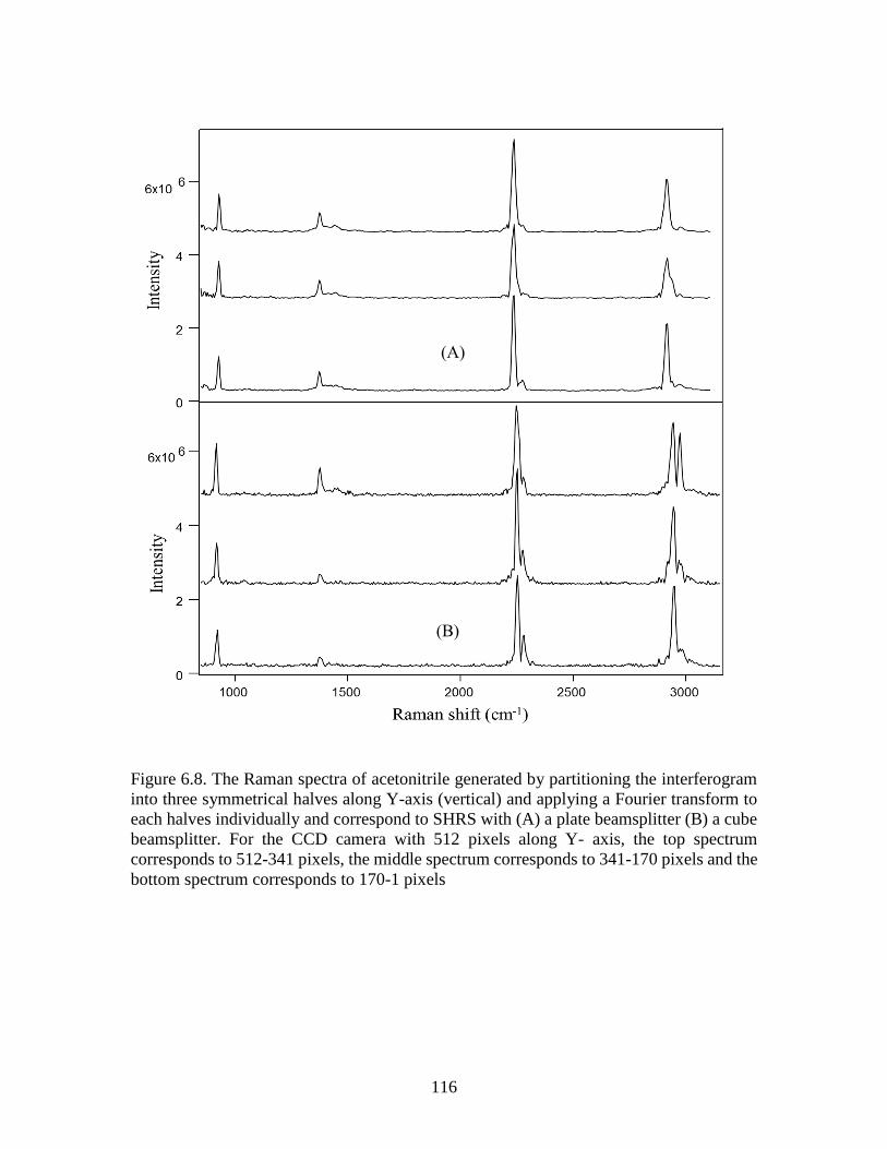
116
Figure 6.8. The Raman spectra of acetonitrile generated by partitioning the interferogram
into three symmetrical halves along Y-axis (vertical) and applying a Fourier transform to
each halves individually and correspond to SHRS with (A) a plate beamsplitter (B) a cube
beamsplitter. For the CCD camera with 512 pixels along Y- axis, the top spectrum
corresponds to 512-341 pixels, the middle spectrum corresponds to 341-170 pixels and the
bottom spectrum corresponds to 170-1 pixels
(A)
(B)

117
Figure 6.9. SHRS Raman spectrum of cyclohexane measured over (A) wide spectral range
(B) limited spectral range using 254 nm bandpass filter. The spectra were acquired using 9
mW, 244 nm laser with 10 s acquisition time. Inset: the cyclohexane’s interferogram
measured over (C), wide spectral range (D) limited spectral range. The arrows above each
interferograms refer to the appropriate intensity axis for that spectrum. The spectra and
interferogram cross sections are offset vertically for clarity.

118
Appendix A
Permission to Reprint Chapter 3

119
Appendix B
Permission to Reprint Chapter 5