STUDY OF THE EFFECTS OF OBSTACLES IN LIQUEFIED NATURAL GAS

(LNG) VAPOR DISPERSION USING CFD MODELING

A Thesis

by

ROBERTO EDUARDO RUIZ VASQUEZ

Submitted to the Office of Graduate Studies of Texas A&M University

in partial fulfillment of the requirements for the degree of

MASTER OF SCIENCE

August 2012

Major Subject: Safety Engineering

2

Study of the Effects of Obstacles in Liquefied Natural Gas (LNG) Vapor Dispersion

using CFD Modeling

Copyright 2012 Roberto Eduardo Ruiz Vásquez

STUDY OF THE EFFECTS OF OBSTACLES IN LIQUEFIED NATURAL GAS

(LNG) VAPOR DISPERSION USING CFD MODELING

A Thesis

by

ROBERTO EDUARDO RUIZ VASQUEZ

Submitted to the Office of Graduate Studies of Texas A&M University

in partial fulfillment of the requirements for the degree of

MASTER OF SCIENCE

Approved by:

Chair of Committee, M. Sam Mannan

Committee Members, Charles J. Glover Cesar O. Malave Head of Department, Charles J. Glover

August 2012

Major Subject: Safety Engineering

iii

ABSTRACT

Study of the Effects of Obstacles in Liquefied Natural Gas (LNG) Vapor Dispersion

using CFD Modeling. (August 2012)

Roberto Eduardo Ruiz Vásquez, B.S., Pedro Ruiz Gallo University, Peru

Chair of Advisory Committee: Dr. M. Sam Mannan

The evaluation of the potential hazards related with the operation of an LNG

terminal includes possible release scenarios with the consequent flammable vapor

dispersion within the facility; therefore, it is important to know the behavior of this

phenomenon through the application of advanced simulation tools. Computational Fluid

Dynamic (CFD) tools are often used to estimate the exclusion zones in an event of

accidental LNG spill. In practice these releases are more likely to occur in the confines

of complex geometries with solid obstacles such as LNG terminals, and LNG processing

plants.

The objective of this research is to study the effects that different obstacles have

over the LNG vapor dispersion and the safety distance reduction caused by enhanced

mixing. Through parametric analysis it is demonstrated that height, width and shape of

the obstacles play an important role in the vapor concentration reduction. The findings of

this research may be applied in the design stage of an LNG terminal, to improve the

design of passive barriers, and for designing better layout configurations for storage

iv

tanks. Simulations results performed with FLACS (Flame Acceleration Simulator), a

CFD solver, confirmed that these applications help to reduce safety distances.

v

DEDICATION

To my parents Mario and Lila, for their motivation and advices during all this

time, I will always be proud of being their son.

To my brother and sisters, Mario, Karla and Cecilia, who always believed in me.

To Isabel an especial person in my life, who is my partner and support in difficult

times.

vi

ACKNOWLEDGEMENTS

I would like to express my sincere gratitude to my advisor Dr. Sam Mannan, for

his support and guidance throughout the course of my graduate studies and for giving me

the opportunity to work on such an interesting topic.

I also would like to acknowledge to Dr. Subramanya Nayak for his excellent

guidance and knowledge in computational fluid dynamics.

I would like to thank to Dr. Charles Glover and Dr. César Malavé, for serving as

members of my advisory committee, for their time and suggestions in the development

of this research.

Thanks also go to Towanna Arnold, Donna Startz and Valerie Green for making

the paperwork easier during my time at Texas A&M University.

Finally, thanks to my family for their encouragement and love during all this

process.

vii

NOMENCLATURE

LNG Liquefied Natural Gas

CFD Computational Fluid Dynamics

FLACS Flame Acceleration Simulator

t Time

T Temperature

LFL Lower Flammability Limit

UFL Upper Flammability Limit

MKOPSC Mary Kay O’Connor Process Safety Center

NFPA National Fire Protection Association

viii

TABLE OF CONTENTS

Page

ABSTRACT .............................................................................................................. iii

DEDICATION .......................................................................................................... v

ACKNOWLEDGEMENTS ...................................................................................... vi

NOMENCLATURE .................................................................................................. vii

TABLE OF CONTENTS .......................................................................................... viii

LIST OF FIGURES ................................................................................................... xi

LIST OF TABLES .................................................................................................... xiv

CHAPTER

I BACKGROUND ON LNG .................................................................. 1

1.1 LNG definition ............................................................................. 1 1.2 LNG safety hazards ...................................................................... 2

1.2.1 Cryogenic hazards ............................................................. 2 1.2.2 Vapor-cloud fire ................................................................ 3 1.2.3 Pool fire ............................................................................. 4 1.2.4 Torch fire ........................................................................... 5 1.2.5 Rapid phase transition ....................................................... 6 1.2.6 Confined space explosion .................................................. 6

1.3 Standards and regulations ............................................................ 6 1.3.1 DOT 49 CFR 193 .............................................................. 6 1.3.2 NFPA 59A ......................................................................... 7 1.3.3 U.S. Coast guard (USCG) regulations .............................. 7

1.4 Consequence analysis requirements ............................................ 7 1.4.1 Estimation of the vapor cloud fire exclusion zone ............ 8 1.4.2 Estimation of the pool fire thermal exclusion zone .......... 8

1.5 Dispersion modeling and models classification ........................... 9 1.5.1 Dispersion modeling ......................................................... 9 1.5.2 Dispersion models classification ...................................... 11

1.5.2.1 Workbooks/correlation models .......................... 12 1.5.2.2 Shallow layer models ......................................... 12

ix

CHAPTER Page

1.5.2.3 Integral models ................................................... 12 1.5.2.4 CFD models ........................................................ 13 1.6 LNG experiments ........................................................................ 14

1.6.1 Large scale experiments: Falcon tests ............................... 14 1.6.2 Medium and small scale experiments ............................... 16 1.6.2.1 BA-Hamburg trials ............................................... 16 1.6.2.2 MKOPSC experiments ......................................... 16 1.6.2.3 Other wind tunnel experiments ............................ 19 II INTRODUCTION ................................................................................ 21

2.1 Motivation .................................................................................... 21 2.2 Objectives .................................................................................... 21 2.3 Methodology ............................................................................... 22 2.4 Relationship with previous research in MKOPSC ....................... 24

III FLACS CAPABILITIES AND VALIDATION .................................. 27 3.1 Capabilities of FLACS in dispersion modeling ........................... 28 3.2 Mathematical models used in FLACS ........................................ 28 3.2.1 Dispersion model .............................................................. 29 3.2.2 LNG pool model ............................................................... 33 3.3 Validation of FLACS against Falcon 1 test ................................. 39 3.3.1 Computational geometry and meshing ............................. 39 3.3.2 Simulation set up .............................................................. 41 3.3.3 Simulation results ............................................................. 42

IV PARAMETRIC ANALYSIS AND SIMULATION ............................... 45 4.1 Simulation set up .......................................................................... 45 4.2 Vapor cloud behavior on different parameters ............................ 47

4.2.1 Shape effect ...................................................................... 47 4.2.2 Height effect ..................................................................... 49 4.2.3 Width effect ...................................................................... 51 4.2.4 Roughness effect .............................................................. 53 4.2.5 Wind velocity effect ......................................................... 55

4.3 Parametric analysis ...................................................................... 57 4.3.1 Analysis of pool release case ........................................... 60 4.3.2 Analysis of jet release case ............................................... 66

V POTENTIAL APPLICATIONS ............................................................ 72

x

CHAPTER Page

5.1 Analysis of aspect ratio and porosity ........................................... 72 5.2 Special applications ...................................................................... 78

5.2.1 Storage tanks’ layout ........................................................ 78 5.2.2 Dike design ....................................................................... 81

VI CONCLUSIONS AND FUTURE WORK .......................................... 86

6.1 Conclusions .................................................................................. 86 6.2 Future work ................................................................................... 88

REFERENCES .......................................................................................................... 89

VITA ......................................................................................................................... 94

xi

LIST OF FIGURES

Page

Fig. 1.1 Vapor cloud fire in China lake ............................................................... 4

Fig. 1.2 LNG pool fire......................................................................................... 5

Fig. 1.3 LNG vapor dispersion phenomena ........................................................ 11

Fig. 1.4 Falcon 1 test configuration .................................................................... 15

Fig. 1.5 Position of measurement instrumentation in MKOPSC 2008 experiments (Data report of MKOPSC LNG spill tests: 2005-2009) .... 18

Fig. 1.6 Pit with wooden vapor fences used in MKOPSC experiments

(Data report of MKOPSC LNG spill tests: 2005-2009) ........................ 18 Fig. 1.7 Flow around a cube normal to the flow in a wind tunnel ...................... 19 Fig. 1.8 Flow around a cylinder normal to the flow in a wind tunnel. ................ 20

Fig. 2.1 Research methodology ........................................................................... 24

Fig. 2.2 Relationship of this research with previous work in LNG vapor dispersion at MKOPSC .......................................................................... 26

Fig. 3.1 Computational geometry generated in FLACS for Falcon1 test ........... 40

Fig. 3.2 Detail of meshing and refinement on the simulation domain. ............... 41

Fig. 3.3 FLACS validation against experimental data and FLUENT simulation. .............................................................................................. 44

Fig. 4.1 Location of the source and measurement points for gas concentration

in the cases of: cube (a) and cylinder (b) ............................................... 46 Fig. 4.2 Shape effect on vapor cloud for cube (a) and cylinder (b). ................... 48

Fig. 4.3 Concentration values along the centerline for cube and cylinder .......... 49

xii

Page

Fig. 4.4 Height effect on vapor cloud for a 3m cube (a) and increased height of cube to 6m (b) ......................................................................... 50

Fig. 4.5 Concentration values and reduction efficiency for cube and cylinder ... 51

Fig. 4.6 Width effect on vapor cloud for a 3m cube (a) and increased width of cube to 6m (b) ................................................................................... 52

Fig. 4.7 Concentration values and concentration reduction for cube and cylinder with increased width ................................................................ 53

Fig. 4.8 Cloud shape for the cube with roughness 0.0002 (a) and 0.03 (b) ........ 54

Fig. 4.9 Concentration values and concentration reduction for cube and cylinder with different roughness values ............................................... 55

Fig. 4.10 Wind velocity effect for a velocity of 1.5 m/s (a) and 6 m/s (b) ........... 56

Fig. 4.11(a) Pareto chart with effects and significance of parameters at downwind distance: x = 3m. .................................................................. 61

Fig. 4.11(b) Pareto chart with effects and significance of parameters at

downwind distance: x = 82.5m .............................................................. 62 Fig. 4.12 Surface plots of parameter interaction at distance: x = 3m.................... 64

Fig. 4.13 Surface plots of parameter interaction at distance x = 82.5m ............... 65

Fig. 4.14(a) Pareto chart with effects and significance of parameters at downwind distance: x = 3m ................................................................... 66

Fig. 4.14(b) Pareto chart with effects and significance of parameters at

downwind distance: x = 82.5m .............................................................. 67 Fig. 4.15 Surface plots for parameter interaction at distance: x = 3m .................. 70

Fig. 4.16 Surface plots for parameter interaction at distance: x = 82.5m ............. 71

Fig. 5.1 Linear tank’s arrangement for aspect ratio and porosity analysis ......... 73

Fig. 5.2 Flammability contours through tanks with three different aspect ratios: (a) 1, (b) 1.5, and (c) 2 ..................................................... 75

xiii

Page

Fig. 5.3 Concentration reductions at different aspect ratios and porosities at 50m from the storage area border line ................................................... 76

Fig. 5.4 Flammability contours through tanks with three different aspect ratios

(staggered layout) .................................................................................. 79 Fig. 5.5 Comparison of flammability contours at different tank’s layout,

with aspect ratio =2, at t = 750 s ............................................................ 80 Fig. 5.6 Comparison between two different dike designs,

dike 1: 110 x 110 x 5 m, dike 2: 85 x 85 x 8 m ..................................... 82 Fig. 5.7 Pool formation within dike 2 at time 600 seconds................................. 83

Fig. 5.8 Comparison between safety distances with the two different analyzed dikes ........................................................................................ 84

Fig. 5.9 Safety distance reduction with two different dike dimensions .............. 85

xiv

LIST OF TABLES

Page

Table 1.1 Physical properties of methane .............................................................. 2

Table 3.1 Relationship between Monin-Obukhov length and atmospheric stability. .................................................................................................. 30

Table 3.2 Wind profile parameters: Ls, Zs, and h (adapted from Bosch & Weterings, 2005; Golder, 1972; and Han et al., 2000). ..................... 31 Table 4.1 Simulation details for parametric analysis in pool release case. ............ 58

Table 4.2 Simulation details for parametric analysis in jet release case. ............... 59

Table 4.3 Parameter values for pool and jet releases. ............................................ 60

Table 4.4 Parameter contribution in the concentration reduction for pool release case at distances: x = 3 m and x = 82.5 m ................................. 63 Table 4.5 Parameter contribution in concentration reduction for jet release case at distances: x = 3 m and x = 82.5 m ................................. 68 Table 5.1 Concentration reduction percentage at different tanks’ layout .............. 81

1

CHAPTER I

BACKGROUND ON LNG

1.1 LNG DEFINITION

Liquefied Natural Gas (LNG) is an odorless, clear cryogenic liquid produced by

cooling natural gas to about 111 Kelvin (K). In its liquid state, the volume of LNG is

about 600 times less than its gaseous state. This reduction in volume allows economical

long distance transportation of LNG by ships to LNG terminals. In these terminals, LNG

is reconverted to its gaseous state to be used in houses, industries, and power plants

(EIA, 2009).

The LNG composition is mainly 95% methane; however, it also contains ethane,

propane and other heavier hydrocarbons. An important property of cold LNG vapor is

that it is heavier than air by a factor of 1.5; therefore, LNG spills results initially into

heavy gas clouds. Table 1.1 shows the main physical properties of methane.

____________ This thesis follows the style of the Journal of Loss Prevention in the Process Industries.

2

Table 1.1 Physical properties of methane (adapted from white paper: LNG pool fire

modeling-MKOPSC, 2008):

Property Value Units

Molecular Weight 16.04 kmol/kg

Freezing point 90.00 K

Boiling point (B.P) 111.70 K

Liquid density at B.P 450.00 kg/m3

Critical temperature 190.60 K

Critical pressure 4.64E+06 Pa

1.2 LNG SAFETY HAZARDS

Following potential hazards are identified in the case of an LNG release in a

facility: cryogenic hazards, vapor c8loud fire, pool fire, torch fire, rapid phase transition,

and confined space explosion (MKOPSC, 2008).

These hazards are explained in detail in the paragraphs that follow.

1.2.1 Cryogenic hazards

This type of hazard is created because LNG has to be stored and transported at

very low temperatures, around 111 K. At these below freezing temperatures there are

negative effects on a living tissue.

3

Also, the containment and structural materials containing the LNG can be

damaged and fail by embrittlement. Therefore, special attention is needed in selecting

adequate materials to withstand cryogenic temperatures. For instance, structures with 5-

9% of nickel steel are required in LNG tanks and other process components in contact

with the LNG (Cormier et al., 2009).

1.2.2 Vapor-cloud fire

In the case of a release, a vapor cloud is generated by the LNG boiling and

mixing with the surrounding air. When the cloud is first dispersed it is heavier than air,

then it is further mixed and diluted with more air as it goes downwind. Flammable

limits of the LNG cloud range from 5 to 15% in volume concentration, and it becomes

hazardous when during its traveling path an ignition source is found. If this flammable

cloud ignites, the resulting flame will propagate through the cloud and then back to the

source. Figure 1.1 shows an example of vapor cloud fire from the China Lake

experiments. Vapor cloud fire can cause severe burns to people in its influence zone, and

also it could damage equipment depending on the exposure time (Raj, 2007).

4

Fig 1.1. Vapor cloud fire in China lake (Raj, 2007)

1.2.3 Pool fire

LNG releases of sufficient flow rate and time could create a pool on the ground.

In the case of ignition it will create a pool fire. As can be seen in figure 1.2, the effects of

a pool fire are localized but it has a longer duration in comparison with a vapor cloud

fire; therefore, it is possible that the pool fire will remain and expand if a spill continues

feeding the pool (Qiao et al., 2006).

5

Fig. 1.2. LNG pool fire (Raj, 2005)

1.2.4 Torch fire

When a release comes from pressurized containment, a spray with liquid droplets

is formed. In the case of ignition, a torch fire is developed leading to direct flame with

radiant heating. In comparison with pool fires, torch fires present the same type of

hazard, but a torch fire is often greater than a pool fire; because the torch fire tends to

produce a larger flame.

6

1.2.5 Rapid phase transition

This phenomenon has been observed in the case of LNG release on or under

water, with a characteristic spontaneous generation of vapor as the cold LNG is

vaporized from heat gained from the spill surface, and with a flameless explosion.

The hazard potential of rapid phase transitions can be severe; however, they will not

propagate further than in the immediate vicinity of the spill area (Qiao et al., 2006).

1.2.6 Confined space explosion

This type of hazard occurs when the vapor cloud traveling downwind finds a

confined space, where in the case of ignition the accumulated vapor could lead to an

explosion. The damage caused by this explosion could be small or large depending on

whether the pressure limit of a building is exceeded.

1.3 STANDARDS AND REGULATIONS

1.3.1 DOT 49 CFR 193

This U.S. Federal standard was promulgated by the Department of

Transportation (DOT) under the title: 49 CFR 193, “Liquefied Natural Gas Facilities:

Federal Safety Standards”. This regulation covers siting requirements, design and

construction, equipment, operations, maintenance, fire protection, and security.

Regarding the safety requirements in an LNG facility, an impounding system is

necessary as well as calculations of vapor dispersion and thermal exclusion zones to

ensure public safety beyond a given facility’s fence line.

7

1.3.2 NFPA 59A

The National Fire Protection Association (NFPA) covers information related to

safety and security in process systems, storage areas, piping systems handling LNG

through the NFPA 59A: “Standard for the Production, Storage, and Handling of

Liquefied Natural Gas (LNG)”. Impounding systems that can contain a possible LNG

spill, as well as dispersion and thermal exclusion zones, also are required under NFPA

59A. Exclusion zones extend from the point of the release to the distance reached by the

vapor cloud in terms of the half Lower Flammability Limit (LFL).

1.3.3 U.S. Coast guard (USCG) regulations

This regulation entitled as “Liquid Flammable Gases,” is related to tanker design

and facility sitting. It determines how to transport LNG safely and requires the use of

manuals where ships operate. Safety rules also are required for specific ports to reduce

accident risk.

1.4 CONSEQUENCE ANALYSIS REQUIREMENTS

Vapor cloud fires and pool fires are two main hazards in an LNG facility, which

have a delayed and immediate potential of ignition, respectively. Regulations such as

NFPA 59A and 49 CFR 193 provide procedures to analyze the consequences of these

hazards in an LNG facility, allowing the design engineer to apply creative solutions to

mitigate catastrophic events.

8

1.4.1 Estimation of the vapor cloud fire exclusion zone

Regulations such as 49 CFR 193 require the estimation of pool fire and vapor

cloud safety distances through simulation tools (U.S. Department of Transportation,

2002). This regulation allows using software such as DEGADIS and FEM3A to perform

vapor dispersion simulations; while for pool fire simulations the allowed software is

LNGFIRE3.

NFPA 59A defines “accidental design spill” as the most representative and

likely-to-occur spill; based on historical experience and special features in an LNG

facility. Design spills must be used as inputs in consequence analysis of an LNG facility

and its surrounding area.

The spill volume is calculated using the following equation:

Spill Volume = [(Spill Time) × (Flow Rate)] + Pipe Drainage (1.1)

Definition of a design spill is basically the same in 49 CFR 193 regulation, with

exception of the process transfer area. The use of a continuous release is present in both

NFPA 59A and 49 CFR 193 standards.

1.4.2 Estimation of the pool fire thermal exclusion zone

In the event of a pool fire, people and property could be severely affected by the

radiation and contact with flames; therefore, determination of fire thermal exclusion

zone is necessary and required by U.S regulations. The estimation of this exclusion zone

9

has different approaches depending on the assumed scenario involved, although the

equations to calculate them are similar.

Requirements for modeling hazard scenarios are given by 49 CFR 193 and

NFPA 59A (section 2) regulations, and they are focused on large volume LNG storage

areas. LNGFIRE simulation model is required by NFPA to calculate thermal radiation

distances, and its predictions are based on calculation of basic flame geometry and

surface radiation flux. Other alternative models are available, and they have been

validated by experimental data taking into account the same physical factors.

Regulations such as the European EN 1473:1997 describe maximum thermal

radiation flux at the property boundary in an LNG facility, with values of 5 kW/m2 for

urban areas, and 1.5 kW/m2 for critical areas.

1.5 DISPERSION MODELING AND MODELS CLASIFICATION

1.5.1 Dispersion modeling

The modeling of the vapor dispersion phenomena is mainly due to two main

steps: the source term and vapor dispersion. For this research the source term is modeled

by a pool formation from an LNG spill; on the other hand, the vapor dispersion describes

the physical process of the gas entrainment in the air and its posterior dilution.

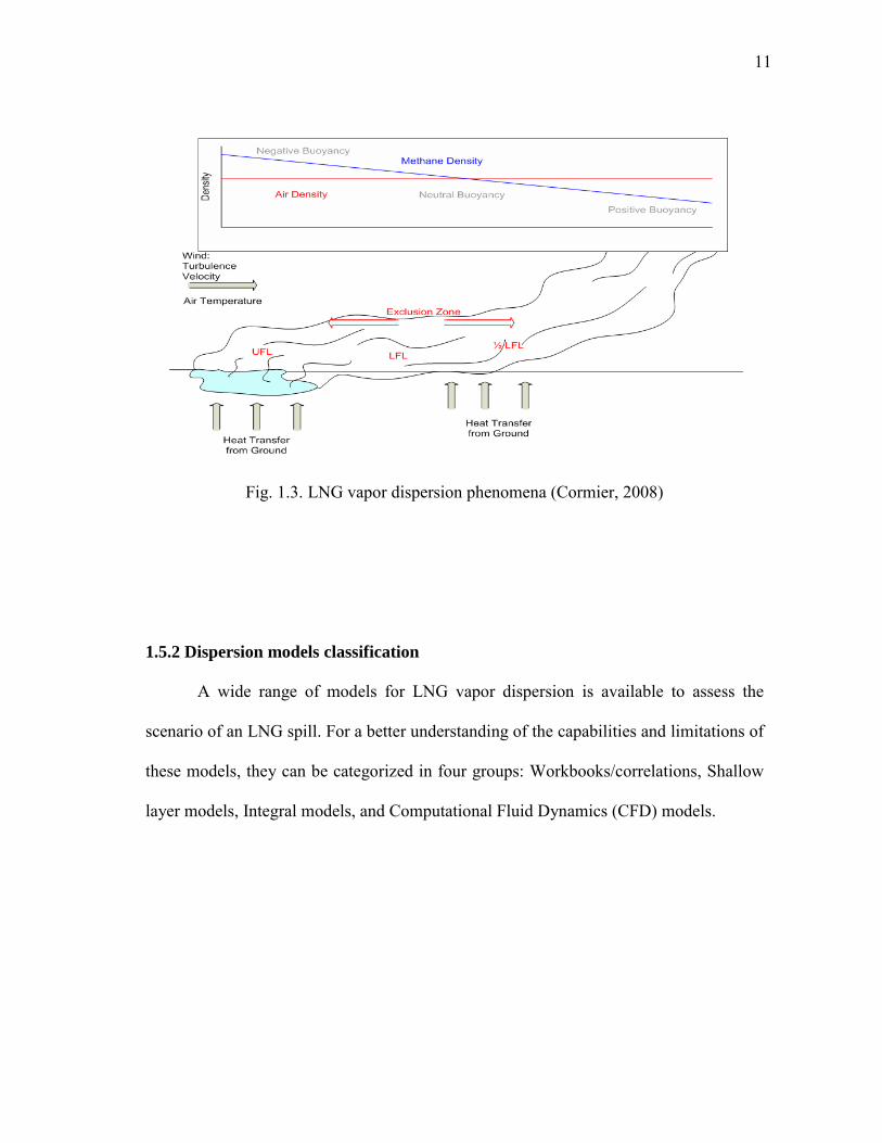
Figure 1.3 describes the phenomena involved in vapor dispersion. The source

term represents the evaporation rate for a given release scenario. The most common

scenario is the pool formation due to a continuous LNG release in a confined area. The

evaporation rate depends mainly on the heat transfer between the liquid pool and the

10

contacted surface. In the case of a release on ground, the evaporation rate will decrease

over time, because the freezing effect of the ground in contact with the cold LNG. If the

pool is formed on water, the evaporation rate will be more continuous, and it will depend

on the turbulence created during the release (Cormier, 2008).

Once the source term is initiated, the phenomenon of vapor dispersion downwind

follows. In the case of LNG, the dispersion follows a heavier-than-air gas behavior,

because its density and cold temperature.

At the beginning, the evaporation is caused by the heat transfer from the

surroundings, with a quick vapor expansion and negative buoyancy effects. Then, the

wind entrainment creates a horizontal mixing and dilution of the vapor. In this stage, the

vapor has a neutral buoyancy but as it travels downstream it becomes positive buoyant.

Atmospheric conditions also play an important role; for instance, during unstable

atmospheric conditions the buoyancy turbulence is present, while during stable

conditions the turbulence is negligible (Cormier, 2008).

Figure 1.3 also indicates the flammable region of LNG, which ranges from 5%

(Lower Flammability Limit, LFL) to 15% (Upper Flammability Limit, UFL). The

concept of exclusion zone or safety distance is defined as the point when the LNG gas

mixture is below the Lower Flammability Limit (LFL); therefore, after that distance the

vapor cloud will not ignite.

The purpose of this section was to explain briefly the phenomena involved in the

dispersion modeling; the equations for pool formation and vapor dispersion are

explained in detail in Chapter III.

11

Fig. 1.3. LNG vapor dispersion phenomena (Cormier, 2008)

1.5.2 Dispersion models classification

A wide range of models for LNG vapor dispersion is available to assess the

scenario of an LNG spill. For a better understanding of the capabilities and limitations of

these models, they can be categorized in four groups: Workbooks/correlations, Shallow

layer models, Integral models, and Computational Fluid Dynamics (CFD) models.

12

1.5.2.1 Workbooks/correlation models

This type of model uses empirical relations to solve two given quantities. The

model expresses the spreading rate in terms of correlations between downstream

distance and atmospheric stability. The main advantages of this model are its simplicity

and quick application; however, it can only be applied to simple scenarios because it

presents limitations in complex situations (Crowl & Louvar, 2002).

1.5.2.2 Shallow layer models

They have a combination of some features of integral and CFD models. For a

dense gas simulation, depth-averaged variables are used to predict the flow behavior.

This model is physically realistic and ideal to simulate dispersion over sloping terrain,

because they are less empirical than integral models but easier to use than CFD models.

However, they need more computational time in comparison with integral models; for

that reason, they are not broadly used in commercial applications and are more popular

for research purposes (Hankin, 2003).

1.5.2.3 Integral models

Differential equations are used in these models to describe the integral properties

of a flow. In the case of heavy gas clouds, this model uses a cylindrical box considering

radius and volume properties varying over time. For this reason, this model is also

known as a box model.

13

Source and dispersion are commonly used separately in integral models; for the

case of LNG, the source is often modeled as a pool. For the case of dispersion, this

model allows different properties such as wind speed, surface roughness and

atmospheric stability, but these properties are modeled as constant over time (Spicer &

Havens, 1987).

Some advantages of using this model are its good prediction capability and its

quick run on the simulated scenarios. For this reason, they are broadly used for hazard

assessments. The main disadvantage of these models is that they usually do not take into

account obstacles or non-flat terrain in the calculation; therefore, sometimes the results

obtained with these models are conservative. Some examples of common integral

models include SLAB, DEGADIS, and PHAST (Puttock, 1987).

1.5.2.4 CFD models

This type of model develops a numerical solution using Navier-Stokes equations

for three dimensional time-dependent flow equations. Its main advantage is the inclusion

of the effects of complex geometries, such tanks or dikes, in the simulation solution on

flow and dispersion. The approach in simulating vapor dispersion is more realistic and

accurate than other models (Chan, 1992). The main disadvantage of this model is the

required simulation time, which can be a few hours or many days, depending on the

complexity of the scenario and computational meshing involved. Another disadvantage

is the relative difficulty during the set up process and the significant computer resources

14

needed; for this reason, this type of simulation must be performed by an experienced

user (Chan, 1994).

Some examples of CFD models widely used are FEM3A, FLUENT, CFX, and

FLACS. Most of them have been validated against full scale or wind tunnels

experiments.

1.6 LNG EXPERIMENTS

1.6.1 Large scale experiments: Falcon tests

The most significant field trial experiments of LNG release in the presence of

obstructions are the Falcon trials undertaken in 1987. The Falcon tests were large scale

experiments developed in 1987 by Lawrence Livermore National Laboratories at

Frenchman Flat, Nevada. The intention of the tests were to evaluate the effectiveness of

vapor barriers on mitigating the hazard distance produced in an eventual LNG release

and also to provide broad data for future validation studies (Brown et al., 1990).

Five LNG spills were created with volumes from 20 m3 to 63 m3 onto a water

pond equipped with a water circulation system to stimulate rapid vaporization of the

LNG and to assure that the evaporation rate was as close as possible to the spill rate.

An uniform LNG distribution on the pond was provided by a spill “spider” system,

which consisted of a main pipe with 4 smaller pipes in its extreme; each small pipe had

0.11 m in diameter and was spaced 90 degrees between each other.

A vapor fence was constructed around the water pond using fiberglass material,

with dimensions of 44 m by 88 m and a height of 8.7 m. A billboard structure with

15

dimensions of 17.1 m wide and 13.3 m height, was located upwind the water pond in

order to simulate the turbulence effect of a storage tank inside the fence. The

experimental setup of the Falcon 1 test is shown in Figure 1.4.

Temperature and gas concentration values along the path of the vapor cloud were

of special interest in this experiment. An array of sensors for these parameters were

located in stations at 50 m, 150 m, and 250 m downwind the water pond; at heights of 1

m, 5 m, 11 m and 17 m above to the ground.

Fig. 1.4. Falcon 1 test configuration (Gavelli et al., 2008)

16

1.6.2 Medium and small scale experiments

In previous years, a series of medium and small scale experiments have been

performed to analyze the behavior of vapor dispersion including the presence of

obstacles. Some of the most relevant experiments carried out are explained below.

1.6.2.1 BA-Hamburg trials

These experiments were carried out by the Meteorological Institute at the

University of Hamburg. Open wind tunnel was used to study several configurations

during the BA-Hamburg trials, under scenarios of instantaneous and continuous releases.

Some of these configurations include crosswind canyons, sloping terrain,

semicircular fence placed upwind or downwind from a release, and a fence completely

surrounding a release (Coldrick et al., 2010). The fences were located downwind from

the release, perpendicular or in angle with the wind direction.

These experiments provided of useful data on dense gas dispersion for further studies

and validation purposes.

1.6.2.2 MKOPSC experiments

From the years 2005 to 2009, six series of small and medium scale experiments

were performed by MKOPSC and TEEX, at the Brayton Fire Training Field (BFTF).

During the development of these experiments, LNG containing 98-99.8% methane was

spilled inside three different concrete pits. The pits contained water inside them, with the

purpose to promote a constant amount of LNG vaporization, equal to the LNG discharge

17

rate. In order to reduce the vertical fluid momentum at the moment of the discharge, a

metal plate was located under the pipe discharge end.

Weather conditions were measured before and during the tests; for instance

humidity, wind direction and velocity, atmospheric temperature and pressure. Also,

other parameters of interest for vapor dispersion, such as gas concentration and

temperature were also measured at different locations and heights along the path of the

vapor cloud. Figure 1.5 shows the position of the poles with the measurement

instrumentation over the predicted path of the vapor cloud, using the setup for the

experiments of the year 2008 (MKOPSC, 2010).

In the experiments performed from the years 2007 to 2009, wooden boards with

a height of 6 feet were located around the pits. The reason was to simulate the effect of

vapor fences in retaining the LNG vapor inside the pits. The experiment results

demonstrated that vapor fences hold up the vapor cloud increasing the turbulence effects

inside the pit and for that reason, they help to reduce significantly the safety distance

downwind.

Figure 1.6 illustrates the pit with wooden vapor fences around it. Also, poles with

measurement instruments and the metal plate under the discharge pipe are showed.

18

Fig. 1.5. Position of measurement instrumentation in MKOPSC 2008 experiments (Data

report of MKOPSC LNG spill tests: 2005-2009).

Fig. 1.6. Pit with wooden vapor fences used in MKOPSC experiments (Data report of

MKOPSC LNG spill tests: 2005-2009).

1

23

45

6

7

8

11

12

13

14

15

17

(0,0)(50,0)

(-50,0)

Large Pit33 ft by 21 ft

(10 m by 6.4 m)

33 ft

21 ft

(0,-33)

(0,67)

19

1.6.2.3 Other wind tunnel experiments

Previous wind tunnel and full scale experiments were developed in order to

evaluate the effects that simple geometries, such as cube and cylinder, have over the

vapor dispersion. Robins and Castro first addressed this topic in 1977, through wind

tunnel experiments analyzing the process involved in plume dispersion in the vicinity of

a cube, finding flow patterns and concentration values downwind (Robins & Castro,

1977). Further experiments were developed in 1993 (Martinuzzi & Tropea, 1993) and in

2003 (Mavroidis et al., 2003).

With regard to the full scale experiments, Ogawa and Oikawa developed field

studies in 1982, intended to study the cavity wake behind a cube with different wind

directions (Ogawa & Oikawa, 1982). Also Macdonald studied the effects of an array of

these geometries in 1998 (Macdonald et al, 1982). Figures 1.7 and 1.8 show the flow

around cube and cylinder geometries in wind tunnel experiments (Mavroidis et al.,

2003).

Fig 1.7. Flow around a cube normal to the flow in a wind tunnel (Mavroidis et al., 2003)

20

Fig 1.8. Flow around a cylinder normal to the flow in a wind tunnel (Mavroidis et al., 2003)

21

CHAPTER II

INTRODUCTION

2.1 MOTIVATION

The design of an LNG (Liquefied Natural Gas) terminal and facility requires the

evaluation of the potential hazards related with its operation, which includes possible

release of LNG, resulting in flammable vapor dispersing within the facility (NFPA,

2009). Safety distances are required to prevent damage outside the facilities in the case

of an LNG release, and regulations such as 49 CFR 193 and standard NFPA 59A require

the application of advanced simulation tools to assess safety distances for accidental

release scenarios.

Several studies in vapor dispersion have been performed in the past; however,

there are few studies about the effects of passive barriers in reducing the safety distance

by using CFD (Computational Fluid Dynamic) models. This research has the purpose to

fill this gap.

2.2 OBJECTIVES

The main goal of this research is to acquire a better understanding about the

effects that different geometries (obstacles) may have over LNG vapor dispersion, and

how much the safety distance could be reduced in presence of these obstacles. To

accomplish these objectives, commercial CFD software FLACS (Flame Acceleration

22

Simulator) is used; given its ability to accurately simulate the dispersion of an LNG

vapor cloud (Hansen et al., 2010).

The main objectives of this research include:

To develop a CFD model tool that can be used for simulating LNG vapor

dispersion through obstacles.

Validation of developed model against a large scale experiment (Falcon 1 test).

To perform a parametric analysis over the main parameters involved in vapor

dispersion to determine their significance in vapor concentration reduction.

To develop a methodology to assess the vapor concentration reduction through

the study of tank aspect ratios and porosities within an LNG storage area.

Application of a CFD model to assess two specific cases: a better design for

dikes, as well as a better layout configuration for storage tanks in an LNG

facility. The goal of both applications was to obtain a reduction in the vapor

concentration, reducing the safety distance.

2.3 METHODOLOGY

The method used in this research includes the validation of the Flame

Acceleration Simulator (FLACS) in accurately simulating LNG vapor dispersion. For

validation purposes, large scale experimental data from the Falcon tests, and small scale

experimental data from the MKOPSC tests are used. Large scale experiments considered

spill volumes of about 40 m3 per release while small scale that amount was about 5 m3.

23

The next step is to study the effects of the obstacles in vapor dispersion. The

main geometries found in an LNG facility (for instance, in an LNG terminal) are tanks

and buildings. In this analysis they will be represented as solid cylinders and cubes; the

exact details of these geometries will be not considered. In future, the methodology

developed in this study can be easily applied to a specific detailed geometry.

Concentration measurement points were considered downwind of the studied obstacles

to gather vapor concentration values.

In order to know which parameters play a more important role in the vapor

concentration reduction, a parametric analysis will be done. The knowledge gained from

this analysis will then be applied to determine optimal passive barriers and LNG tank

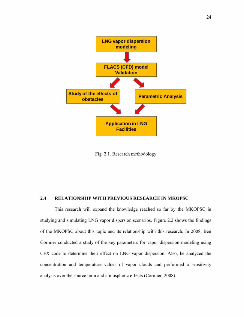
farm layout. Figure 2.1 shows the steps that are used to achieve the research objectives.

24

Fig. 2.1. Research methodology

2.4 RELATIONSHIP WITH PREVIOUS RESEARCH IN MKOPSC

This research will expand the knowledge reached so far by the MKOPSC in

studying and simulating LNG vapor dispersion scenarios. Figure 2.2 shows the findings

of the MKOPSC about this topic and its relationship with this research. In 2008, Ben

Cormier conducted a study of the key parameters for vapor dispersion modeling using

CFX code to determine their effect on LNG vapor dispersion. Also, he analyzed the

concentration and temperature values of vapor clouds and performed a sensitivity

analysis over the source term and atmospheric effects (Cormier, 2008).

LNG vapor dispersion

modeling

FLACS (CFD) model

Validation

Parametric Analysis

Application in LNG

Facilities

Study of the effects of

obstacles

25

In 2011, Ruifeng Qi performed a source term study on LNG underwater release.

His research focused on the measurement of the reduction in the safety distance with the

use of vapor fences around a pit, comparing a scenario with-fence versus with-no-fence.

Validation of the experimental data of the MKOPSC using the CFX code was

performed, along with a sensitivity analysis for the mesh size and the source term

turbulence (Qi, 2011).

As mentioned earlier, this research will use the previous findings in order to

analyze the effects of passive barriers in vapor dispersion using CFD code by modifying

the shape, height, and width of passive barriers and also the roughness and wind speed.

Parametric analysis will be used to quantify the effects of obstacles and passive barriers

in vapor dispersion phenomena.

26

Fig 2.2. Relationship of this research with previous work in LNG vapor dispersion at

MKOPSC

Ben Cormier

MKOPSC tests: Concentration &

Temperature analysis

Parameters effect on vapor

dispersion

Sensitivity analysis: Source term &

atmospheric effects

Roberto Ruiz

FLACS validation (large & medium

scale tests)

Parametric analysis for

geometry effects

Propose a new design or

configuration for passive barriers

Ruifeng Qi

Source term study on LNG

underwater release

CFX mesh size & source term

turbulence effects

Findings in MKOPSC tests: Vapor Fences

effect

This study Year 2008 Year 2011

27

CHAPTER III

FLACS CAPABILITIES AND VALIDATION

FLACS is a CFD tool that can address complex scenarios and it is commonly

used for dispersion modeling of flammable and toxic gases. This tool was developed in

1980 at the Department of Science and Technology at Christian Michelsen Institute

(CMI); some years later they established Gexcon as a consultant company which

currently holds the property rights of the FLACS code (Gexcon AS, 2011).

Previous studies have been carried out reviewing many aspects of FLACS such

as the studies performed in 2004 (Hanna et al., 2004) and in 2008 (Hansen et al., 2008).

Also, independent studies by the Health and Safety Laboratory have been done. Lately,

a validation of FLACS against gas dispersion experiments was performed following the

Model Evaluation Protocol (Hansen et al., 2010).

On October 7, 2011, FLACS was approved to be used for modeling vapor

dispersion scenarios by The Pipeline and Hazardous Materials Safety Administration

(PHMSA) of the U.S. Department of Transportation. In this manner, FLACS is the only

approved model for simulating LNG dispersion scenarios for facility siting in the United

States (Gexcon website, 2012).

This chapter will explain the capabilities and mathematical models used by

FLACS; for instance, the dispersion model which solves the Reynolds-averaged-Navier-

Stokes (RANS) equations on a non-uniform Cartesian grid. In the case of the pool

model, governing equations and the expressions for a spreading pool are presented.

28

3.1 CAPABILITIES OF FLACS IN DISPERSION MODELING

This software presents many advantages in simulating different scenarios such as

dense or buoyant gases in open or obstructed environments. Documentation for

validation of FLACS is available from different papers or from Gexcon website, and the

results obtained are in good agreement with experimental data.

A feature that makes FLACS distinct from other CFD models is its distributed

porosity model for small and sub-grid scale obstacles; which allows a relative rapid

simulation in comparison with other CFD codes. In general purpose CFD codes the

source model is not usually available; however, FLACS includes source models for

evaporating pools as well as for flashing and high-pressure releases.

Set up options for different boundary conditions also are available in this

software, which takes into account atmospheric stability classes and surface roughness in

the simulation domain. Furthermore, FLACS includes a suitable turbulence model and

solution methods such as wall functions, pressure correction algorithms and spatial

discretization schemes.

3.2 MATHEMATICAL MODELS USED IN FLACS

LNG dispersion modeling involves two main steps: the pool source and its

posterior vapor dispersion. This section will cover the mathematical equations used by

FLACS to address both phenomena.

29

3.2.1 Dispersion model

FLACS approaches vapor dispersion by solving the Reynolds-averaged-Navier-

Stokes (RANS) equations on a non-uniform Cartesian grid. The model allows including

temperature profiles as a function of Pasquil-Gifford stability classes; and also wind

velocity, turbulence, and surface roughness length (z0) are considered.

Properties of the atmospheric boundary layer on the floor’s surface are

reproduced by using wind boundaries. The buoyancy effects on the atmospheric

boundary layer are explained by the characteristic length scale, which is shown in the

equation 3.1 (Monin & Obukhov, 1954).

(3.1)

In equation, u* is the friction velocity and Hs is the sensible heat flux from the

surface. Stability of the atmospheric boundary can be measured by the value of the

Monin-Obukov length.

Table 3.1 shows the relationship between Monin-Obukov lengths and the atmospheric

stability (Bosch & Weterings, 2005).

30

Table 3.1 Relationship between Monin-Obukhov length and atmospheric stability

(adapted from Bosch & Weterings, 2005).

Monin-Obukhov length Stability Condition

Small negative, -100m < L0 Very unstable

Large negative, -105 < L < -100 Unstable

Very large, L > 105 Neutral

Large positive, 10 < L < 105 Stable

Small positive, 0 < L < 10 Very stable

To estimate the Monin-Obukhov length, FLACS uses the Pasquill stability

classes which indicate the level of turbulence present in the atmosphere. In the initial set

up the user has to include the wind velocity (U0) at a reference height (zref), the Pasquill

stability class, and also the atmospheric roughness length (z0).

The logarithmic velocity profile is given by equation 3.2.

(3.2)

(3.3)

31

In the equation (3.3), u* is the friction velocity and zd is the canopy height.

Term is defined in the next equation:

(3.4)

where = (1 – 16 z/L)1/4 (3.5)

Table 3.2 shows the wind profile parameters used to calculate velocity, k, and ε values at

wind boundaries.

Table 3.2 Wind profile parameters: Ls, Zs, and h (adapted from Bosch & Weterings,

2005; Golder, 1972; and Han et al., 2000).

Pasquill class Stability Boundary layer

height, h Ls Zs

A Unstable 1500 m 33.162 m 1117 m

B Unstable 1500 m 33.258 m 11.46 m

C Slightly unstable 1000 m 51.787 m 1.324 m

D Neutral

1.0 m 0 m

E Slightly stable

- 48.33 m 1.262 m

F Stable

- 31.323 m 19.36 m

32

A simpler way to calculate the Monin-Obukhov length is by Golder’s equation

which uses the values from Table 3.2 (Golder, 1972).

(3.6)

In the case of the wind boundary profiles for turbulent kinetic energy, FLACS

uses the equations proposed by Han et al. (2000) to calculate k and ε.

The heated air close to the ground surface causes unstable boundary layers, because the

air density close to the ground is lower than the air above, generating unstableness.

For unstable boundary layers (A, B, and C), the inlet profiles are:

(3.7)

and

(3.8)

33

The heat velocity w* is given by the next expression:

(3.9)

For neutral and stable boundary layers; relations between friction velocity and

Monin-Obukhov length are given:

(3.10)

and

(3.11)

3.2.2 LNG pool model

The governing equations for a spreading pool in FLACS takes into account the

friction, heat and mass transfer. This model has been validated for a spreading pool with

and without obstacles under different conditions: adiabatic, on water, and on soil.

For cryogenic liquids such as LNG, the heat transfer is dominated by the heat

from the substrate where the pool is formed. The equation 3.12 gives the heat transfer

from all types of ground at non-boiling conditions:

34

(3.12)

Equation 3.12 is only valid for conductive heat transfer; some parameters are: αg

which is the thermal diffusivity, λg is the thermal conductivity, tgw is the time when the

pool starts, and is the ground temperature before the ground is wetted.

Besides the conductive heat transfer, there is a convective contribution between

the spreading pool and the ground, which is showed in equation 3.13.

(3.13)

where:

λl: Conductivity

Prl: Prandtl number of the pool liquid

: Ground temperature at the surface.

Therefore, the total heat transfer for pools at non-boiling conditions, and on all

types of ground can be calculated by using the cubic blending function:

35

(3.14)

The term given in equation 3.13 indicates the ground temperature at the

surface, which can be calculated by the next equation:

(3.15)

When the pool develops on smooth surfaces such as water; instead using the

equations explained above, the boiling heat transfer equations are used. When the

surface temperature where the pool is formed is at least 4 K higher than the boiling point

temperature of the pool liquid, a phenomenon called slight superheat occurs. Nucleate

boiling of a pool is assumed for slight superheats; and Cooper’s correlation is used to

calculate the heat transfer generated:

(3.16)

and

pr = psat/pc (3.17)

36

where:

psat: Saturation pressure

pc: Critical pressure

Then, the nucleate boiling heat transfer is used instead of the conductive heat

transfer in the cubic blending function to calculate the total heat transfer.

During the film-boiling regime, expressions for transition boiling and film

boiling heat transfer are used according to (Conrado & Vesovic, 2000):

(3.18)

where the term q˙g,film is the film boiling heat transfer for a fluid in rest.

The convective heat transfer, based on boundary layer theory, is given by the next

expression:

(3.19)

37

Term T+ is given by a two-layer model:

(3.20)

The convective mass transfer is given by the next expression:

(3.21)

where x = Pg/P0

and x+ is calculated by:

(3.22)

The radiative heat transfer caused by the contribution of the sun and surroundings can be

calculated by:

(3.23)

38

where:

w: Albedo

Ɛg : Emission coefficient of the surrounding gas

Ɛp: Emission coefficient of the pool liquid

Σ: Stefan-Boltzmann constant.

The total evaporation rate is given by the sum of the convective mass transfer and

boiling:

(3.24)

where:

(3.25)

The next equation shows the heat transfer due to evaporation:

(3.26)

39

3.3 VALIDATION OF FLACS AGAINST FALCON 1 TEST

Previous validation studies of Falcon tests were performed using CFD tools; for

instance, FLUENT code was used to simulate the Falcon 1 test, providing some of the

necessary parameters to accurately predict this test. Also, a comparison between

experimental and simulation results was provided (Gavelli et al., 2008).

On the other hand, FLACS code was validated against Falcon tests using the

model evaluation database for LNG vapor dispersion, showing reliable results in its

prediction (Hansen et al., 2010).

For the purpose of this research, it is important to demonstrate that the results

obtained by different authors with regard to the Falcon 1 test, can be replicated using

FLACS. By doing this, it can be inferred that the model is reliable and can be applied to

other scenarios involving LNG releases.

This section is going to develop the validation for the Falcon 1 test using

FLACS, and the results obtained are going to be compared with previously reported

results in FLUENT (Gavelli et al., 2008).

3.3.1 Computational geometry and meshing

The Falcon 1 test considered an LNG release inside a water pond surrounded by

vapor fences and a billboard structure located upwind. The details of this experiment

were explained in detail in Chapter I.

40

The simulation domain considered the x axis as horizontal and parallel to the

wind direction, y axis as horizontal in the crosswind direction, and the z axis as vertical.

The origin point was located in the center of the downwind fence, at ground level.

The computational domain considered ranges from -200 m to 300 m in the x-direction,

from -250 m to 250 m in the y-direction, and from 0 m to 50 m in the z-direction.

Water pond, vapor fences, and the billboard were included in the model to take

into account their effects in vapor dispersion. Figure 3.1 shows the computational

geometry generated in FLACS for the Falcon 1 test.

Fig. 3.1. Computational geometry generated in FLACS for Falcon 1 test

41

Meshing process was performed on the domain, with a grid refinement close to

the pool leak and the obstacles considered in the set up.

The total control volumes were 382,000; with Cartesian grid cells about 0.8 x 0.8 x 0.5

m in the refinement zone. Figure 3.2 shows the details of the meshing and refinement on

the simulation domain.

Fig. 3.2. Detail of meshing and refinement on the simulation domain

3.3.2 Simulation set up

Monitor points for measuring vapor concentration were located downwind the

vapor fence, using the same location as in the Falcon 1 experiment. Boundary

conditions, which are a set of differential equations at the boundary of a given domain,

42

were considered for the outlet simulation domain. Wind inflow boundary was assumed

in the x direction (upwind from the vapor fence) and along the y direction. Nozzle

condition was considered for the outflow boundary in the x direction (downwind from

the vapor fence), and also on the top of z direction.

As initial conditions, wind velocity of 1.7 m/s measured at 2 m height. Pasquill

stability class “D” and an ambient temperature of 32.8 ºC were selected. The

aerodynamic roughness length (z0) was 0.03, similar to typical values for flat terrain.

FLACS pool model was used to calculate the pool formed during the LNG spill

and the vaporization rate generated from it. LNG with a composition of 95% methane,

4% ethane and 1% propane was released inside the water pond with a spill rate of 202

kg/s, during a total time of 131 s. The model takes turbulence caused by the LNG

discharge into consideration by a relative turbulence intensity of 0.05, similar to medium

turbulence intensity.

3.3.3 Simulation results

Comparison between the experimental data in Falcon test 1 and the results

obtained with FLUENT (Gavelli et al., 2008) and FLACS (this work) are shown in

Figure 3.3.

The continuous blue line represents the experimental data, while the FLUENT

simulation result is shown by the profile green line. The FLACS simulation result

obtained in this research is shown by the continuous black line.

43

The results obtained with FLACS indicated that the cloud pass over the fence at

approximately a time of 70 s, when it reaches the analyzed concentration measurement

point. Afterwards, the concentration will build up until it reaches 7.5% v/v at a time of

260 s, and then it finally decreases.

Both models (FLACS and FLUENT) showed the same pattern and they are

reasonable accurate despite the under-prediction in the simulation results. The reason for

this under-prediction was the peculiar release conditions during the Falcon 1

experiments, where a high pressure jet was observed, with associated flashing and

aerosol formation. Therefore, it is concluded that the difference between experimental

and simulation results are given because the definition of the source term, rather than a

deficiency with the model.

44

Fig. 3.3. FLACS validation against experimental data and FLUENT simulation

0

2

4

6

8

10

12

14

0 100 200 300 400 500 600 700

Time (s)

Gas concentration (%)

Experimental Fluent simulation

FLACS simulation

Ga

s C

on

cen

tra

tion

(V

ol.

%)

Time (s)

45

CHAPTER IV

PARAMETRIC ANALYSIS AND SIMULATION

The first chapter explained that vapor dispersion modeling includes two main

phenomena: the source term and vapor dispersion. This research is focused on the vapor

dispersion and the effects of the key parameters in reducing the concentration values by

enhancing mixing of LNG vapor with air. Five key parameters were selected and

studied: height, width, and shape of the obstacles as well as ground roughness and wind

velocity (Cormier, 2008).

This chapter is divided in two main sections: vapor cloud behavior under

different parameters, and parametric analysis. The first section explains the different

behavior that a vapor cloud when a variation in the parameters mentioned above is

performed. The second section discusses the parametric analysis performed on the

analyzed parameters and finds the parameters contribution in the concentration

reduction.

4.1 SIMULATION SETUP

Previous wind tunnel experiments studied the behavior and dispersion of heavier-

than-air gases passing through two main obstacles: cube and vertical cylinder (Mavroidis

et al., 2003). Although LNG was not used for these experiments, its properties are

comparable to a heavier-than-air gas; therefore, a similar behavior can be expected.

46

2L

2L

2L

2L

2L

L = 3.0 m

0.5 L

Source

location

Wind

direction

0.5 L

2L

2L

2L

2L

2L

L = 3.0 m

0.5 L

Source

location

Wind

direction

0.5 L

Inside an LNG facility, for instance an LNG terminal, the main obstacles that can

be found are buildings and tanks, which for simulation purposes can be generalized as

cubes and cylinders, respectively. The effects that these obstacles may have over an

LNG vapor dispersion scenario are going to be analyzed by using FLACS code. The

setup for the simulation analysis is similar to the wind tunnel experiments developed by

Mavroidis in 2003, and explained in Chapter I.

The release source was located upwind from the analyzed obstacles, at a distance

2 times larger than their width, which for these simulations was 3 meters. In the same

manner, concentration measurement points were considered downwind from the rear

face of the obstacle, and located at distances 2 times their width, as observed in Figure

4.1.

(a) (b)

Fig. 4.1. Location of the source and measurement points for gas concentration in the

cases of: cube (a) and cylinder (b).

47

4.2 VAPOR CLOUD BEHAVIOR ON DIFFERENT PARAMETERS

For this analysis a base case scenario was considered, with continuous gas

release rate of 4.5 kg/s initiated at the source point, as indicated in Figure 4.1. FLACS

diffuse model was used for the simulations, because it allows a release with low

momentum and velocity, similar to the gas release characteristics in wind tunnels.

Neutral stability conditions were considered with a low wind velocity of 1.5 m/s, and

ground roughness value of 0.03.

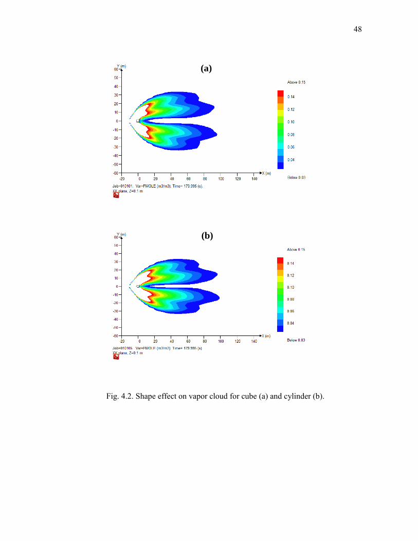
4.2.1 Shape effect

The effect that shape of the obstacles plays on the vapor dispersion was evaluated

by analyzing two different obstacles: cylinder and cube. The simulation results for these

obstacles are shown in Figure 4.2. This figure shows the contours of the flammable

region with a gas concentration from the ½ Lower Flammability Limit (LFL) to the

Upper Flammability Limit (UFL). For LNG vapor the LFL and UFL values are 5 and

15% by volume, respectively. At time t= 180 seconds, it can be seen that the

concentration values downwind from both the cube and cylinder along the centerline are

lower than the ½ LFL value, falling out the flammability region. This region is plotted

with no color, and it is more pronounced for the case of the cube compared with the

cylinder. The reason for this behavior is because cylinders and cubes produce different

flow patterns, causing a faster reattachment of the cloud in the case of cylinder, after the

gas cloud passed through it

48

Fig. 4.2. Shape effect on vapor cloud for cube (a) and cylinder (b).

(b)

(a)

49

Figure 4.3 compares concentration values obtained with the cylinder and cube obstacles

at different distances (in meters) downwind from the obstacles at t= 180 seconds.

Fig. 4.3. Concentration values along the centerline for cube and cylinder.

4.2.2 Height effect

In this case, the height of the obstacles was increased from 3 meters to 6 meters;

however, the width was kept constant at 3meters. Figure 4.4 shows the flammable region

contours of the vapor cloud for the cube case. The wider region (with no color)

downwind from the cube indicates that the concentration values along the centerline

were decreased by augmenting the height of the cube.

0.00E+00

5.00E-03

1.00E-02

1.50E-02

2.00E-02

2.50E-02

3.00E-02

3.50E-02

0 20 40 60 80 100 120 140

Cube

Cylinder

Va

po

r co

nce

ntr

ati

on

(V

ol.

%)

Distance (m)

50

Fig. 4.4. Height effect on vapor cloud for a 3m cube (a) and increased height of cube to

6m (b).

(b)

(a)

51

Figure 4.5 shows the concentration values and the concentration reduction (in

percentage) along the centerline, for the cube and cylinder obstacles. In this case, the

concentration values were decreased by 90% for the cube, while for the cylinder this

reduction was 85%.

Fig. 4.5. Concentration values and reduction efficiency for cube and cylinder.

4.2.3 Width effect

Modification in the obstacles was done by doubling their width from 3m to 6m, but

keeping the height at 3m. A similar behavior as the previous case was obtained. Figure

4.6 shows the comparison between the flammable regions of the vapor clouds, for the

cube case. It is concluded that an increment in the width of the obstacle results in a

0.0

10.0

20.0

30.0

40.0

50.0

60.0

70.0

80.0

90.0

100.0

0.00

0.20

0.40

0.60

0.80

1.00

1.20

Obstacle Height (m)

Vap

or

con

cen

trat

ion

(V

ol.

%)

Co

nce

ntr

atio

n R

ed

uct

ion

(%

)

3m 6m

Cube

3m 6m

Cylinder

52

decrement in the concentration values along the centerline, as indicated by the region

with no color downwind from the cube.

Fig. 4.6. Width effect on vapor cloud for a 3m cube (a) and increased width of cube to

6m (b).

(a)

(b)

53

Figure 4.7 shows the concentration values and concentration reduction (in

percentage) along the centerline for the cube and cylinder cases. The concentration

reduction was 84.5 % for the cylinder and 82.6 % for the cube.

Fig. 4.7. Concentration values and concentration reduction for cube and cylinder with

increased width.

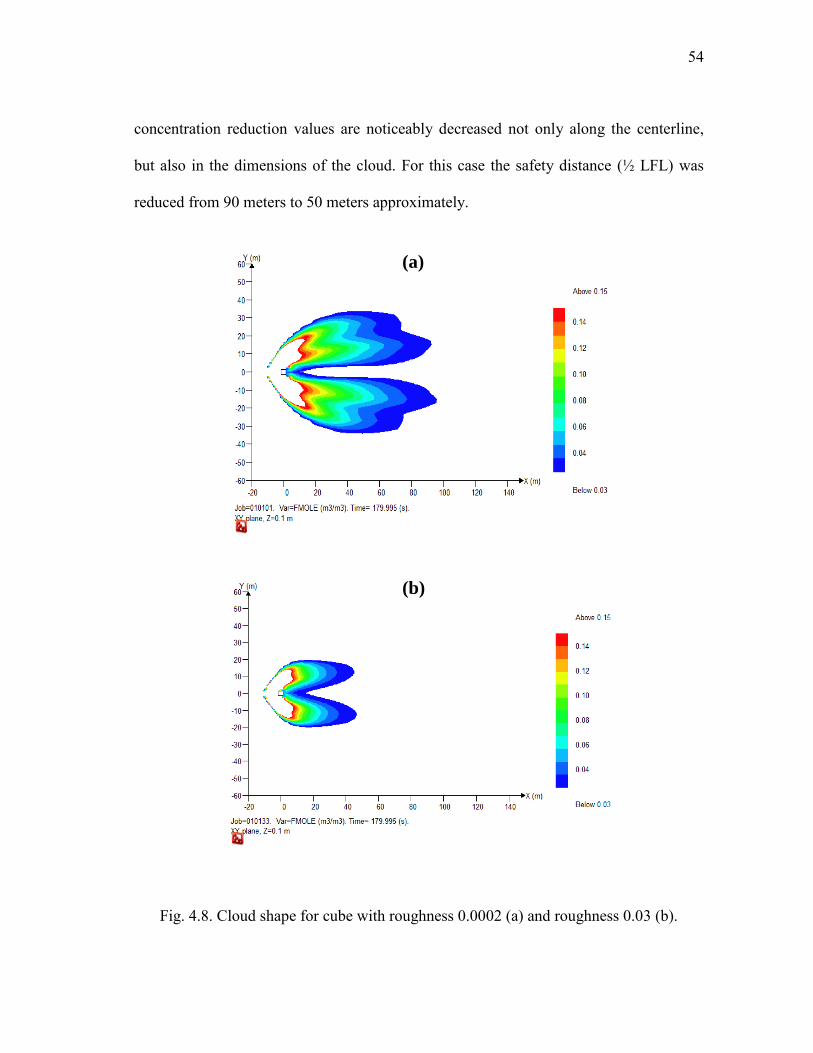
4.2.4 Roughness effect

Roughness is an important parameter in vapor dispersion, because a large

homogeneous roughness can considerably reduce the concentration values downwind

(Petersen, 1990). In this case, Figure 4.8 (a) shows the flammable contours for the vapor

cloud with a roughness value of 0.0002 and (b) with a roughness value of 0.03. The

65.0

70.0

75.0

80.0

85.0

90.0

0.00

0.20

0.40

0.60

0.80

1.00

1.20

Obstacle Width (m)

Co

nce

ntr

atio

n R

ed

uct

ion

(%

)

3m 6m

Cube

3m 6m

Cylinder

Vap

or

con

cen

trat

ion

(V

ol.

%)

54

concentration reduction values are noticeably decreased not only along the centerline,

but also in the dimensions of the cloud. For this case the safety distance (½ LFL) was

reduced from 90 meters to 50 meters approximately.

Fig. 4.8. Cloud shape for cube with roughness 0.0002 (a) and roughness 0.03 (b).

(a)

(b)

55

Figure 4.9 shows the concentration values and the reduction efficiency along the

centerline for the cube and cylinder cases. For the cube, a concentration reduction of 85

% was obtained and for the cylinder this reduction was 80 % when surface roughness

was increased from 0.0002 to 0.03.

Fig. 4.9. Concentration values and concentration reduction for cube and cylinder with

different roughness values.

4.2.5 Wind velocity effect

Also it is important to analyze other parameters unrelated to the geometry of the

obstacles such as the wind velocity. Figure 4.10 shows the effect of wind velocity over

the vapor dispersion for the cube case. A noticeable reduction in the width of the

flammable region is found, and also along the centerline downwind from the cube when

65.0

70.0

75.0

80.0

85.0

90.0

0.00

0.20

0.40

0.60

0.80

1.00

1.20

Obstacle Roughness (m)

Co

nce

ntr

atio

n R

ed

uct

ion

(%

)

0.0002 0.03

Cube

0.0002 0.03

Cylinder

Vap

or

con

cen

trat

ion

(V

ol.

%)

56

the wind velocity was 6 m/s. However, there also are some traces of flammable mixture

on the sides, caused by the separation of the cloud after it passed through the cube.

Fig. 4.10. Wind velocity effect for a velocity of 1.5 m/s (a) and 6 m/s (b).

(a)

(b)

57

4.3 PARAMETRIC ANALYSIS

The previous analysis allowed us to understand the effect of a single parameter

on LNG vapor behavior; however, not a combined effect of all of them. Parametric

analysis allows combining all the levels involved in the vapor dispersion through

obstacles, investigating the effects of each simple factor (parameter) and also the

interaction of them; therefore, it is possible to find the joint effect of the factors on a

given response (Montgomery & Runger, 2006). Different factors that will be

investigated in this section are the same as discussed earlier: height, width, geometry

shape, surface roughness and wind speed.

A special case of 2k factorial design is used in this research. In this design, k

represents the five factors discussed earlier, and they are analyzed at two levels. The 2k

factorial design is applied to two accidental scenarios. In first of these, LNG spilled onto

the ground and pool formation was assumed. In the second scenario an LNG jet was

released. The resulting amounts of simulations were 32 for each case, and they were

compared with a case of dispersion without obstacles, in order to know the difference in

concentration reduction.

Tables 4.1 and 4.2 list all the 32 runs for the pool and jet release cases,

respectively. The symbols – 1 and + 1 represent the low and high levels of the factors;

the table also shows the concentration values without obstacles and with obstacles at 3 m

and 82.5 m downwind the obstacles. Efficiency in concentration reduction also is

showed for these points.

58

Table 4.1 Simulation details for parametric analysis in pool release case

Run Wind Shape Height Width Roughness

Concentration

with no obstacle

Concentration

with obstacle Reduction Efficiency (%)

x = 3m x =

82.5m x = 3m

x =

82.5 m

Effic.

(x=3m)

Effic.

(x=82.5m)

1 -1 -1 -1 -1 -1 0.1786 0.0519 0.0410 0.0107 77.0 79.5

2 1 -1 -1 -1 -1 0.5648 0.0268 0.0405 0.0119 92.8 55.6

3 -1 1 -1 -1 -1 0.1786 0.0519 0.0503 0.0154 71.8 70.3

4 1 1 -1 -1 -1 0.5648 0.0268 0.1298 0.0119 77.0 55.6

5 -1 -1 1 -1 -1 0.1786 0.0519 0.0172 0.0061 90.4 88.2

6 1 -1 1 -1 -1 0.5648 0.0268 0.0325 0.0078 94.2 70.8

7 -1 1 1 -1 -1 0.1786 0.0519 0.0279 0.0081 84.4 84.3

8 1 1 1 -1 -1 0.5648 0.0268 0.0292 0.0082 94.8 69.4

9 -1 -1 -1 1 -1 0.1786 0.0519 0.0277 0.0078 84.5 85.0

10 1 -1 -1 1 -1 0.5648 0.0268 0.0410 0.0204 92.7 23.8

11 -1 1 -1 1 -1 0.1786 0.0519 0.0311 0.0118 82.6 77.2

12 1 1 -1 1 -1 0.5648 0.0268 0.0463 0.0095 91.8 64.7

13 -1 -1 1 1 -1 0.1786 0.0519 0.0073 0.0036 95.9 93.1

14 1 -1 1 1 -1 0.5648 0.0268 0.0064 0.0032 98.9 87.9

15 -1 1 1 1 -1 0.1786 0.0519 0.0103 0.0046 94.2 91.2

16 1 1 1 1 -1 0.5648 0.0268 0.0079 0.0032 98.6 88.0

17 -1 -1 -1 -1 1 0.1912 0.0134 0.0498 0.0086 85.0 95.3

18 1 -1 -1 -1 1 0.4784 0.0385 0.0448 0.0113 90.6 70.5

19 -1 1 -1 -1 1 0.1912 0.0134 0.0579 0.0098 80.5 93.0

20 1 1 -1 -1 1 0.4784 0.0385 0.1134 0.0146 76.3 62.1

21 -1 -1 1 -1 1 0.1912 0.0134 0.0263 0.0073 86.3 45.1

22 1 -1 1 -1 1 0.4784 0.0385 0.0192 0.0021 96.0 94.6

23 -1 1 1 -1 1 0.1912 0.0134 0.0326 0.0089 82.9 33.6

24 1 1 1 -1 1 0.4784 0.0385 0.0398 0.0042 91.7 89.2

25 -1 -1 -1 1 1 0.1912 0.0134 0.0261 0.0068 86.3 49.0

26 1 -1 -1 1 1 0.4784 0.0385 0.0144 0.0043 97.0 88.8

27 -1 1 -1 1 1 0.1912 0.0134 0.0329 0.0078 82.8 41.6

28 1 1 -1 1 1 0.4784 0.0385 0.0375 0.0054 92.2 86.0

29 -1 -1 1 1 1 0.1912 0.0134 0.0095 0.0047 95.0 65.1

30 1 -1 1 1 1 0.4784 0.0385 0.0006 0.0003 99.9 99.2

31 -1 1 1 1 1 0.1912 0.0134 0.0095 0.0052 95.0 60.7

32 1 1 1 1 1 0.4784 0.0385 0.0022 0.0010 99.5 97.4

59

Table 4.2 Simulation details for parametric analysis in jet release case

Wind Shape Height Width Roughness

Concentration no

obstacle

Concentration with

obstacle

Reduction Efficiency

(%)

x = 3m x =

82.5m x = 3m

x = 82.5

m

Effic.

(x=3m)

Effic.

(x=82.5m)

1 -1 -1 -1 -1 -1 0.0935 0.0276 0.0199 0.0060 78.8 78.3

2 1 -1 -1 -1 -1 0.0733 0.0343 0.0321 0.0085 56.2 75.2

3 -1 1 -1 -1 -1 0.0935 0.0276 0.0863 0.0327 7.7 -18.4

4 1 1 -1 -1 -1 0.0733 0.0343 0.0625 0.0230 14.8 33.0

5 -1 -1 1 -1 -1 0.0935 0.0276 0.0323 0.0169 65.5 38.9

6 1 -1 1 -1 -1 0.0733 0.0343 0.0246 0.0051 66.4 85.2

7 -1 1 1 -1 -1 0.0935 0.0276 0.0791 0.0328 15.5 -18.9

8 1 1 1 -1 -1 0.0733 0.0343 0.0627 0.0315 14.5 8.2

9 -1 -1 -1 1 -1 0.0935 0.0276 0.0169 0.0061 81.9 77.9

10 1 -1 -1 1 -1 0.0733 0.0343 0.0265 0.0054 63.8 84.2

11 -1 1 -1 1 -1 0.0935 0.0276 0.0325 0.0134 65.2 51.5

12 1 1 -1 1 -1 0.0733 0.0343 0.0353 0.0159 51.9 53.5

13 -1 -1 1 1 -1 0.0935 0.0276 0.0126 0.0078 86.5 71.9

14 1 -1 1 1 -1 0.0733 0.0343 0.0104 0.0056 85.9 83.6

15 -1 1 1 1 -1 0.0935 0.0276 0.0353 0.0104 62.2 62.3

16 1 1 1 1 -1 0.0733 0.0343 0.0199 0.0083 72.9 75.8

17 -1 -1 -1 -1 1 0.0914 0.0282 0.0226 0.0064 75.3 77.3

18 1 -1 -1 -1 1 0.0743 0.0357 0.0309 0.0092 58.4 74.1

19 -1 1 -1 -1 1 0.0914 0.0282 0.0844 0.0339 7.6 -20.1

20 1 1 -1 -1 1 0.0743 0.0357 0.0624 0.0200 15.9 44.1

21 -1 -1 1 -1 1 0.0914 0.0282 0.0221 0.0079 75.8 72.0

22 1 -1 1 -1 1 0.0743 0.0357 0.0307 0.0036 58.7 89.9

23 -1 1 1 -1 1 0.0914 0.0282 0.0794 0.0340 13.2 -20.4

24 1 1 1 -1 1 0.0743 0.0357 0.0669 0.0219 10.0 38.7

25 -1 -1 -1 1 1 0.0914 0.0282 0.0187 0.0071 79.5 74.9

26 1 -1 -1 1 1 0.0743 0.0357 0.0228 0.0063 69.3 82.3

27 -1 1 -1 1 1 0.0914 0.0282 0.0370 0.0146 59.6 48.4

28 1 1 -1 1 1 0.0743 0.0357 0.0418 0.0132 43.7 63.2

29 -1 -1 1 1 1 0.0914 0.0282 0.0127 0.0067 86.1 76.1

30 1 -1 1 1 1 0.0743 0.0357 0.0093 0.0052 87.5 85.5

31 -1 1 1 1 1 0.0914 0.0282 0.0299 0.0126 67.3 55.4

32 1 1 1 1 1 0.0743 0.0357 0.0184 0.0081 75.2 77.3

60

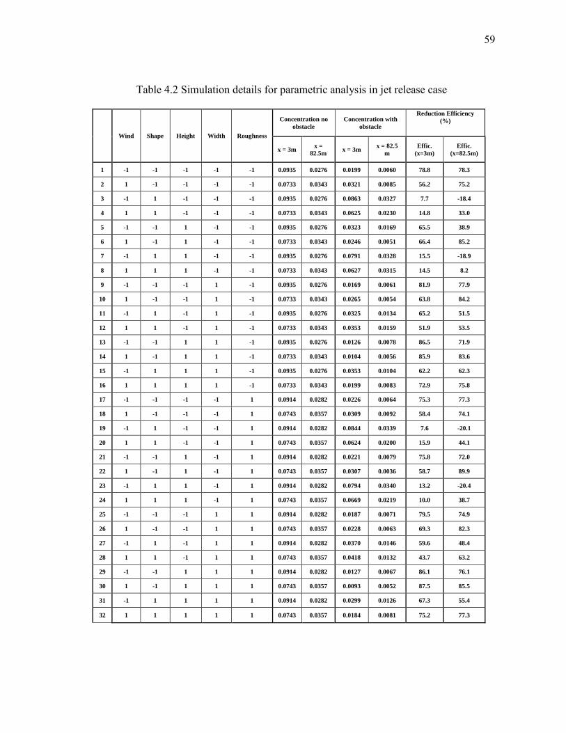
The maximum and minimum values for each analyzed parameter are shown in Table 4.3.

These values were selected according with worst case and most favorable case scenarios.

Table 4.3 Parameter values for pool and jet releases

Parameter Min (-) Max (+)

Wind 1.5 m/s 6 m/s

Shape Cube Cylinder

Height 3.0 m 6 m

Width 3.0 m 6 m

Roughness 0.0002 0.03

4.3.1 Analysis of pool release case

This research uses a statistical experimental design tool called Design Expert 8.7

for statistical analysis. Figure 4.11 shows a Pareto chart, the result of statistical analysis

for LNG pool scenario. Here the objective was to determine the significant effect of each

parameter and their combination in reducing downwind concentration of LNG vapor.

Pareto chart ranks the effects of the parameters by their magnitude, as a multiple

of the standard deviation (t-value). This chart provides confidence about the significant

effects of the parameters (non-zero); for instance, values above the t-Value limit provide

a 95% confidence that certain effects are possibly significant, while values below the t-

Value limit are not likely to be significant. The Bonferroni limit (red line in Pareto chart)

61

approaches to a 95% confidence level; therefore, the effects sufficiently large will pass

this limit and they are almost certainly significant (DeLoach & Ulbrich, 2008).

Generally, it was observed that the height and width of the obstacles compared to

other factors play a more significant role in reducing LNG concentration downwind and

enhancing the turbulence when vapor is mixing with the air.

Fig. 4.11(a). Pareto chart with effects and significance of parameters at downwind

distance: x = 3 m

Design-Expert® SoftwareConcentration Reduction

A: Wind Veloc.B: ShapeC: HeightD: WidthE: Roughness

Positive Effects Negative Effects

Pareto Chart

t-V

alu

e o

f |E

ffe

ct|

Rank

0.00

2.30

4.59

6.89

9.18

11.48

1 2 3 4 5 6 7 8 9 10 11 12 13 14 15 16 17 18 19 20 21 22 23 24 25 26 27 28 29 30 31

Bonf erroni Limit 3.55369

t-Value Limit 2.0639

C

DA

B

BDBC

AC

A: Wind

B: Shape

C: Height

D: Width

E: Roughness

(a)

62

Fig. 4.11(b). Pareto chart with effects and significance of parameters at downwind

distance: x = 82.5 m

From Figure 4.11(a) it is founded that the height, width, and wind velocity, play

the most important role in the reduction of the vapor concentration, close to the obstacle

(at 3m). When the concentration measurement is done far away point from the obstacle

(at 82.5 m), a combination effect of wind velocity and ground roughness becomes more

important, as can be seen in Figure 4.11 (b).

Table 4.4 shows the effect list of the parameters analyzed and their contribution

in the concentration reduction at 3 m and 82.5 m downwind from the obstacle.

Design-Expert® Software(Concentration Reduction) 2̂.2

A: Wind Veloc.B: ShapeC: HeightD: WidthE: Roughness

Positive Effects Negative Effects

Pareto Chart

t-V

alu

e o

f |E

ffe

ct|

Rank

0.00

2.69

5.37

8.06

10.74

1 2 3 4 5 6 7 8 9 10 11 12 13 14 15 16 17 18 19 20 21 22 23 24 25 26 27 28 29 30 31

Bonf erroni Limit 3.51981

t-Value Limit 2.05553

AE

C

DA

E

A: Wind

B: Shape

C: Height

D: Width

E: Roughness

(b)

63

Table 4.4 Parameter contribution in the concentration reduction for pool release case at

distances: x = 3 m and x = 82.5 m

Parameter

Contribution in the

concentration reduction (%)

x= 3m x = 82.5m

Height 34 19.8

Width 25.4 7.7

Wind Velocity 23.3 6.8

Shape 5.9 0.5

Roughness 0.1 2.6

Wind Velocity&Roughness 0.2 51.4

Other parameters combination 11.2 11.1

Reduction of vapor concentration values by interaction between two parameters

can be better understood by using surface plots. For instance, Figure 4.12 (a) shows the

efficiency in concentration reduction (in percentage) when the wind velocity or height of

the obstacle were modified. By increasing, either wind velocity or height, the

concentration values can be reduced by about 91%. However, if both parameters are

increased at the same time, a reduction of 97% could be achieved. Figure 4.12 (b) shows

the interaction between height and width of an obstacle. The values were measured at

3m from the rear face of the analyzed obstacle.

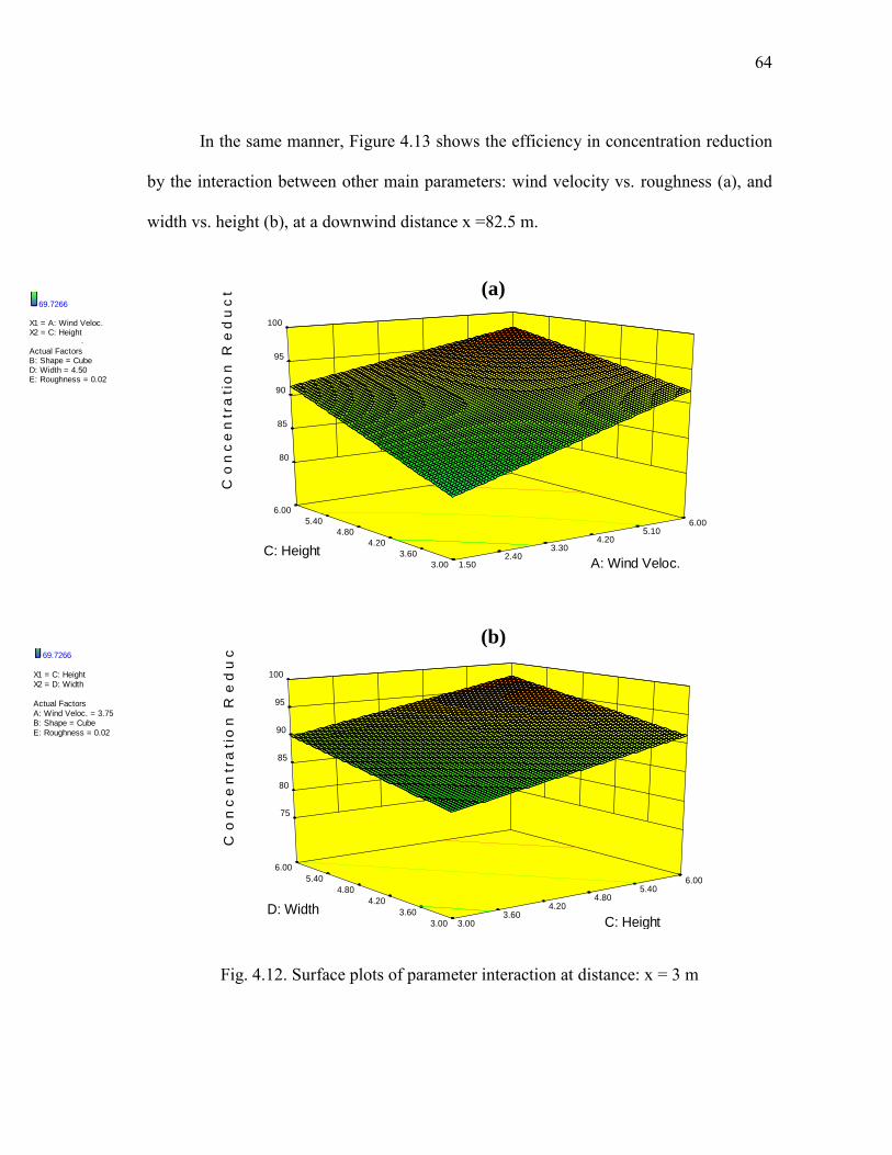
64

In the same manner, Figure 4.13 shows the efficiency in concentration reduction

by the interaction between other main parameters: wind velocity vs. roughness (a), and

width vs. height (b), at a downwind distance x =82.5 m.

Fig. 4.12. Surface plots of parameter interaction at distance: x = 3 m

Design-Expert® SoftwareFactor Coding: ActualConcentration Reduction

99.8782

69.7266

X1 = A: Wind Veloc.X2 = C: Height

Actual FactorsB: Shape = CubeD: Width = 4.50E: Roughness = 0.02

3.00

3.60

4.20

4.80

5.40

6.00

1.50 2.40

3.30 4.20

5.10 6.00

80

85

90

95

100

C

on

ce

ntr

ati

on

Re

du

cti

on

A: Wind Veloc. C: Height

Design-Expert® SoftwareFactor Coding: ActualConcentration Reduction

99.8782

69.7266

X1 = C: HeightX2 = D: Width

Actual FactorsA: Wind Veloc. = 3.75B: Shape = CubeE: Roughness = 0.02

3.00

3.60

4.20

4.80

5.40

6.00

3.00 3.60

4.20 4.80

5.40 6.00

75

80

85

90

95

100

C

on

ce

ntr

ati

on

Re

du

cti

on

C: Height D: Width

(a)

(b)

65

Fig. 4.13. Surface plots of parameter interaction at distance: x = 82.5 m

Design-Expert® SoftwareFactor Coding: ActualOriginal Scale (median estimates)Concentration Reduction

99.189

23.7896

X1 = A: Wind Veloc.X2 = E: Roughness

Actual FactorsB: Shape = CubeC: Height = 4.50D: Width = 4.50

0.00 0.01

0.01 0.02

0.02 0.03

0.03

1.50

2.40

3.30

4.20

5.10

6.00

30

40

50

60

70

80

90

C

on

ce

ntr

ati

on

Re

du

cti

on

A: Wind Veloc.

E: Roughness

Design-Expert® SoftwareFactor Coding: ActualOriginal Scale (median estimates)Concentration Reduction

99.189

23.7896

X1 = C: HeightX2 = D: Width

Actual FactorsA: Wind Veloc. = 3.75B: Shape = CubeE: Roughness = 0.02

3.00

3.60

4.20

4.80

5.40

6.00

3.00

3.60

4.20

4.80

5.40

6.00

30

40

50

60

70

80

90

C

on

ce

ntr

ati

on

Re

du

cti

on

C: Height

D: Width

(a)

(b)

66

4.3.2 Analysis of jet release case

A similar approach as described above was used for the jet release case. The

effects and significance of the parameters at a distance of 3 m and 82.5 m downwind the

obstacles are shown in Figure 4.14, using Pareto charts.

Fig. 4.14 (a). Pareto chart with effects and significance of parameters at downwind

distance: x = 3 m.

Design-Expert® SoftwareConcentration Reduction

A: Wind Veloc.B: ShapeC: HeigthD: WidthE: Roughness

Positive Effects Negative Effects

Pareto Chart

t-V

alu

e o

f |E

ffe

ct|

Rank

0.00

1.50

2.99

4.49

5.99

7.48

8.98

10.47

11.97

13.47

14.96

1 2 3 4 5 6 7 8 9 10 11 12 13 14 15 16 17 18 19 20 21 22 23 24 25 26 27 28 29 30 31

Bonf erroni Limit 3.51981

t-Value Limit 2.05553

B

D

BD

C CD

A: Wind

B: Shape

C: Height

D: Width

E: Roughness

(a)

67

Fig. 4.14 (b). Pareto chart with effects and significance of parameters at downwind

distance: x = 82.5 m (b)

Design-Expert® SoftwareConcentration reduction

A: Wind VelocB: ShapeC: HeightD: WidthE: Roughness

Positive Effects Negative Effects

Pareto Chartt-

Va

lue

of

|Eff

ec

t|

Rank

0.00

2.80

5.60

8.40

11.19

1 2 3 4 5 6 7 8 9 10 11 12 13 14 15 16 17 18 19 20 21 22 23 24 25 26 27 28 29 30 31

Bonf erroni Limit 3.536

t-Value Limit 2.05954

B

D

BD

A

ADAB

A: Wind

B: Shape

C: Height

D: Width

E: Roughness

(b)

68

From the Figure 4.14 (a), it is evident that the shape, width, and a combination of

shape and width are the most important parameters in the reduction of the concentration

values close to the obstacle. Shape of the obstacle plays an important role in the

concentration reduction downwind; this behavior is different from the pool case, where

the shape of the obstacle doesn’t play an important role in the concentration reduction.

The other important parameters are the height and width of the obstacle, similar

compared with the pool case; however, with less contribution.

When the concentration is measured far away from the obstacle (at 82.5 m),

besides the importance of the shape and width, a combined effect of both plays an

important role in the concentration reduction, as shown in Figure 4.14 (b).

Table 4.5 summaries the effect list of the analyzed parameters and their

contribution in the concentration reduction at 3 m and 82.5 m downwind the obstacle.

Table 4.5 Parameter contribution in concentration reduction for jet release case at

distances: x = 3m and x = 82.5m

Parameter

Contribution in concentration

reduction (%)

x= 3m x = 82.5m

Shape 45.4 42.0

Width 34.5 20.6

Height 1.8 0.0

Wind Velocity 0.9 10.5

Shape&Width 11.7 13.7

Other parameters combination 11.2 13.2

69

Figure 4.15 and Figure 4.16 show the surface plots by interaction between the

main parameters in the concentration reduction at a downwind distance x = 3m and

x=82.5 m. Figure 4.15 (a) shows the efficiency in concentration reduction (in

percentage) when either the wind velocity or the width of the obstacle are modified. By

increasing the wind velocity, a concentration reduction of 90% can be obtained, while if

the roughness is increased the concentration reduction is 82%. If both parameters are

increased, the total reduction achieved is 92%. The same analysis could be done for

Figure 4.15 (b) where an interaction between width and height of an obstacle is showed.

In the same way, Figure 4.16 shows the efficiency in concentration reduction by

the interaction between other main parameters: wind velocity vs. height (a), and width

vs. wind velocity (b); at a downwind distance x =82.5 m.

70

Fig. 4.15. Surface plots for parameter interaction at distance: x = 3 m

Design-Expert® SoftwareFactor Coding: ActualConcentration Reduction

87.4939

7.63371

X1 = D: WidthX2 = E: Roughness

Actual FactorsA: Wind Veloc. = 3.75B: Shape = CubeC: Heigth = 4.50

0.00 0.01

0.01 0.02

0.02 0.03

0.03

3.00

3.60

4.20

4.80

5.40

6.00

0

20

40

60

80

100

C

on

ce

ntr

ati

on

Re

du

cti

on

D: Width E: Roughness

Design-Expert® SoftwareFactor Coding: ActualConcentration Reduction

87.4939

7.63371

X1 = C: HeigthX2 = D: Width

Actual FactorsA: Wind Veloc. = 3.75B: Shape = CubeE: Roughness = 0.02

3.00

3.60

4.20

4.80

5.40

6.00

3.00

3.60

4.20

4.80

5.40

6.00

0

20

40

60

80

100

C

on

ce

ntr

ati

on

Re

du

cti

on

C: Heigth D: Width

(b)

(a)

71

Fig. 4.16. Surface plots for parameter interaction at distance: x = 82.5 m

Design-Expert® SoftwareFactor Coding: ActualConcentration reduction

89.9025

-20.4293

X1 = A: Wind VelocX2 = C: Height

Actual FactorsB: Shape = CubeD: Width = 4.50E: Roughness = 0.02

3.00

3.60

4.20

4.80

5.40

6.00

1.50

2.40

3.30

4.20

5.10

6.00

0

20

40

60

80

100

C

on

ce

ntr

ati

on

re

du

cti

on

A: Wind Veloc C: Height

Design-Expert® SoftwareFactor Coding: ActualConcentration reduction

89.9025

-20.4293

X1 = A: Wind VelocX2 = D: Width

Actual FactorsB: Shape = CubeC: Height = 4.50E: Roughness = 0.02

3.00

3.60

4.20

4.80

5.40

6.00

1.50

2.40

3.30

4.20

5.10

6.00

0

20

40

60

80

100

C

on

ce

ntr

ati

on

re

du

cti

on

A: Wind Veloc D: Width

(b)

(a)

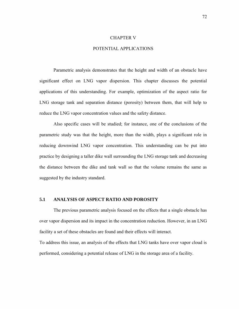
72

CHAPTER V

POTENTIAL APPLICATIONS

Parametric analysis demonstrates that the height and width of an obstacle have

significant effect on LNG vapor dispersion. This chapter discusses the potential

applications of this understanding. For example, optimization of the aspect ratio for

LNG storage tank and separation distance (porosity) between them, that will help to

reduce the LNG vapor concentration values and the safety distance.

Also specific cases will be studied; for instance, one of the conclusions of the

parametric study was that the height, more than the width, plays a significant role in

reducing downwind LNG vapor concentration. This understanding can be put into

practice by designing a taller dike wall surrounding the LNG storage tank and decreasing

the distance between the dike and tank wall so that the volume remains the same as

suggested by the industry standard.

5.1 ANALYSIS OF ASPECT RATIO AND POROSITY

The previous parametric analysis focused on the effects that a single obstacle has

over vapor dispersion and its impact in the concentration reduction. However, in an LNG

facility a set of these obstacles are found and their effects will interact.

To address this issue, an analysis of the effects that LNG tanks have over vapor cloud is

performed, considering a potential release of LNG in the storage area of a facility.

73

Aspect ratio of an obstacle is defined as the proportional relationship between its

width and its height, as shown in equation 5.1:

(5.1)

On the other hand, porosity area is defined as the proportional relationship

between the void-space and the total space of a determined surface. For this case study,

they were considered tanks in a linear arrangement as indicated in Figure 5.1. The

diameter of the tanks is represented by “d” and the distance between them is represented

by “L”.

Fig. 5.1. Tanks’ linear arrangement for aspect ratio and porosity analysis

d: diameter

L: space between

tanks

Wind

direction

74

Then, the porosity along the x axis is given by the equation 5.2:

(5.2)

The aspect ratio and porosity along the axis are related in this analysis, since an

increase in the tank diameter produces a decrease in the porosity over the analyzed axis.

The aspect ratios considered were 1, 1.5 and 2; while the porosity values obtained were

0.45, 0.38, and 0.34. How the aspect ratio of a tank influences in the concentration

reduction of a vapor cloud has not been previously addressed; therefore, this analysis

will provide new knowledge on this topic.

The release scenario simulated was an LNG leak due to a pipe rupture; the

location of the leak was at x= 20 m, in front of the first tank of the storage area. Pool

formation from the release was assumed, generating a vaporization rate of 110 kg/s for a

total time of 10 minutes. The vapor generated will flow through the tanks from left to

right, because the wind is assumed blowing in that direction with a velocity of 1.5 m/s. A

roughness value of 0.03m was considered along the cloud path.

Figure 5.2 illustrates the flammability contours of the vapor cloud through three

tank aspect ratios: 1, 1.5, and 2, at time t = 600 seconds. In Figure 5.2 can be seen the

different behavior for the flammable contours of the vapor cloud when it passes through

the tanks. It was observed that the distance traveled by the vapor cloud is slightly

reduced when the porosity is reduced (diameter increase).

75

Fig. 5.2. Flammability contours through tanks with three different aspect ratios: (a) 1, (b)

1.5, and (c) 2.

(a)

(b)

(c)

76

A total of nine simulations were performed to combine the three different aspect

ratios and porosities of the tanks. The vapor concentration values were taken at the end

of the centerline of the storage area, and were compared in order to determine the vapor

concentration reduction.

Figure 5.3 illustrates the concentration reductions (difference between

concentrations with obstacles and without obstacles) obtained with the tanks at the

analyzed aspect ratios and porosities along the x axis, measured at a distance of 50 m

from the border line of the storage area.

Fig. 5.3. Concentration reductions at different aspect ratios and porosities at 50 m from

the storage area border line.

78.5

79.0

79.5

80.0

80.5

81.0

81.5

82.0

82.5

83.0

0.300 0.320 0.340 0.360 0.380 0.400 0.420 0.440 0.460

Aspect Ratio 1.5

Aspect Ratio 1

Aspect Ratio 2

Porosity

Co

nce

ntr

ati

o R

edu

ctio

n(%

)

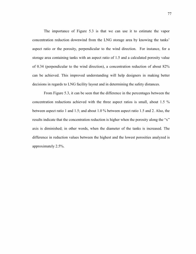
77

The importance of Figure 5.3 is that we can use it to estimate the vapor

concentration reduction downwind from the LNG storage area by knowing the tanks’

aspect ratio or the porosity, perpendicular to the wind direction. For instance, for a

storage area containing tanks with an aspect ratio of 1.5 and a calculated porosity value

of 0.34 (perpendicular to the wind direction), a concentration reduction of about 82%

can be achieved. This improved understanding will help designers in making better

decisions in regards to LNG facility layout and in determining the safety distances.

From Figure 5.3, it can be seen that the difference in the percentages between the

concentration reductions achieved with the three aspect ratios is small, about 1.5 %

between aspect ratio 1 and 1.5; and about 1.0 % between aspect ratio 1.5 and 2. Also, the

results indicate that the concentration reduction is higher when the porosity along the “x”

axis is diminished; in other words, when the diameter of the tanks is increased. The

difference in reduction values between the highest and the lowest porosities analyzed is

approximately 2.5%.

78

5.2 SPECIAL APPLICATIONS

5.2.1 Storage tanks’ layout

Tanks’ layout in an LNG facility is generally linear in arrangement of rows,

similar to the arrangement showed in Fig 5.1. This case study analyzes a proposed new

staggered configuration for the tanks within the storage area. The proposed new

configuration of the tanks is intended to achieve lower concentration values downwind

from the tanks, because of the diminishment in the porosity along the x axis created by

this new tank arrangement. The wind was assumed to be blowing in the x direction from

left to right at a velocity of 1.5 m/s, at neutral atmospheric stability conditions. A typical

roughness of 0.03m was considered along the cloud path.

A scenario of a pipe rupture and LNG leak is assumed to begin at a location x=

20 m at the beginning of the tank storage area. The release time is 10 minutes and pool

formation is assumed, with a vaporization rate of 110 kg/s. The vapor cloud generated

will pass through the tanks from left to right and measurements of the vapor

concentration are taken at the end of the storage area, along the centerline.

Figure 5.4 shows the flammable vapor cloud (5-15% in concentration volume) at a time

t= 650 seconds, for a set of tanks with three different aspect ratios: 1, 1.5, and 2.

79

Fig. 5.4. Flammability contours through tanks with three different aspect ratios

(staggered layout): (a) 1, (b) 1.5, and (c) 2.

(a)

(b)

(c)

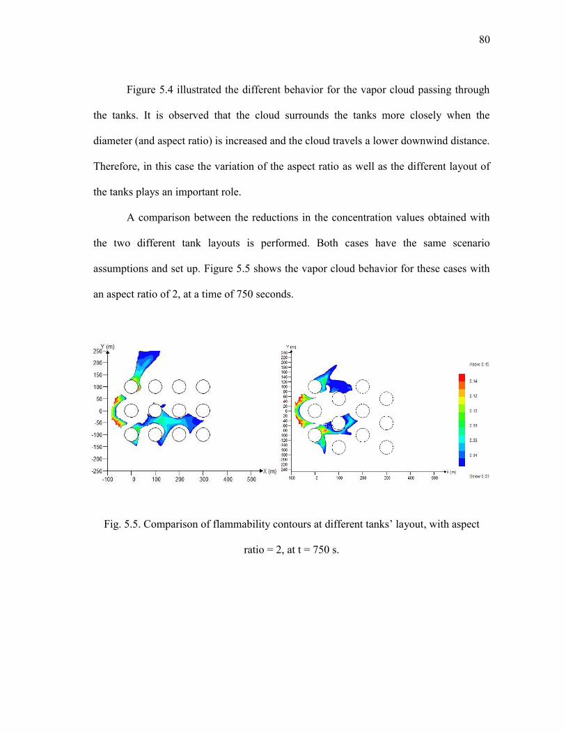
80

Figure 5.4 illustrated the different behavior for the vapor cloud passing through

the tanks. It is observed that the cloud surrounds the tanks more closely when the

diameter (and aspect ratio) is increased and the cloud travels a lower downwind distance.

Therefore, in this case the variation of the aspect ratio as well as the different layout of

the tanks plays an important role.

A comparison between the reductions in the concentration values obtained with

the two different tank layouts is performed. Both cases have the same scenario

assumptions and set up. Figure 5.5 shows the vapor cloud behavior for these cases with

an aspect ratio of 2, at a time of 750 seconds.

Fig. 5.5. Comparison of flammability contours at different tanks’ layout, with aspect

ratio = 2, at t = 750 s.

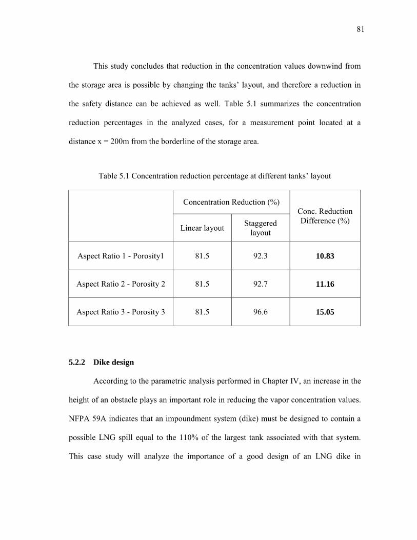
81

This study concludes that reduction in the concentration values downwind from

the storage area is possible by changing the tanks’ layout, and therefore a reduction in

the safety distance can be achieved as well. Table 5.1 summarizes the concentration

reduction percentages in the analyzed cases, for a measurement point located at a

distance x = 200m from the borderline of the storage area.

Table 5.1 Concentration reduction percentage at different tanks’ layout

Concentration Reduction (%) Conc. Reduction Difference (%)

Linear layout Staggered layout

Aspect Ratio 1 - Porosity1 81.5 92.3 10.83

Aspect Ratio 2 - Porosity 2 81.5 92.7 11.16

Aspect Ratio 3 - Porosity 3 81.5 96.6 15.05

5.2.2 Dike design

According to the parametric analysis performed in Chapter IV, an increase in the

height of an obstacle plays an important role in reducing the vapor concentration values.

NFPA 59A indicates that an impoundment system (dike) must be designed to contain a

possible LNG spill equal to the 110% of the largest tank associated with that system.

This case study will analyze the importance of a good design of an LNG dike in

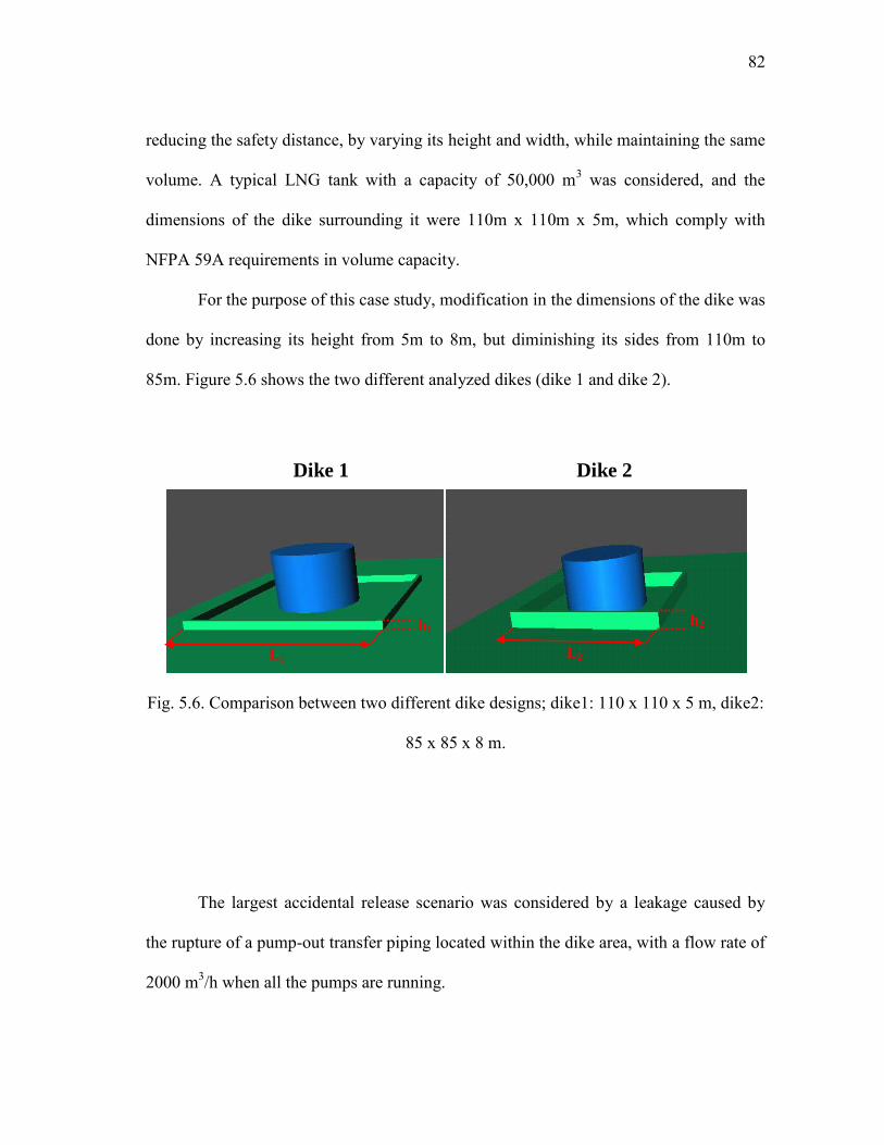
82

reducing the safety distance, by varying its height and width, while maintaining the same

volume. A typical LNG tank with a capacity of 50,000 m3 was considered, and the

dimensions of the dike surrounding it were 110m x 110m x 5m, which comply with

NFPA 59A requirements in volume capacity.

For the purpose of this case study, modification in the dimensions of the dike was

done by increasing its height from 5m to 8m, but diminishing its sides from 110m to

85m. Figure 5.6 shows the two different analyzed dikes (dike 1 and dike 2).

Fig. 5.6. Comparison between two different dike designs; dike1: 110 x 110 x 5 m, dike2:

85 x 85 x 8 m.

The largest accidental release scenario was considered by a leakage caused by

the rupture of a pump-out transfer piping located within the dike area, with a flow rate of

2000 m3/h when all the pumps are running.

h1 h2

L2 L1

Dike 1 Dike 2

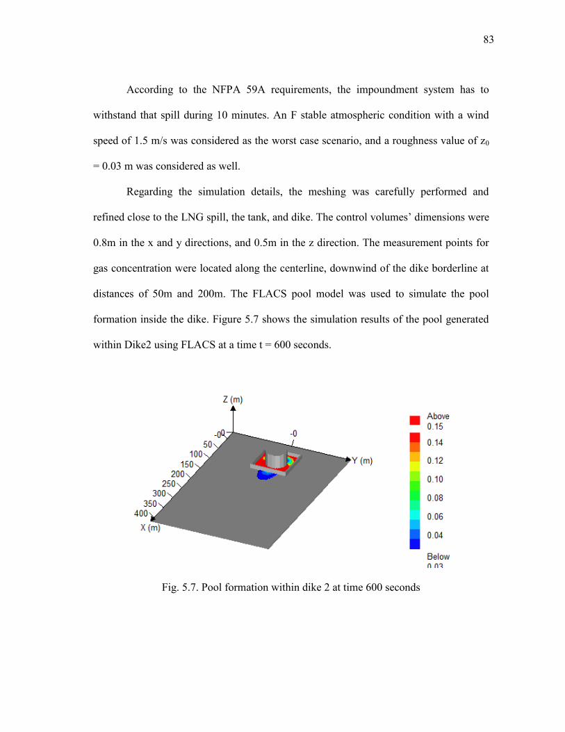
83

According to the NFPA 59A requirements, the impoundment system has to

withstand that spill during 10 minutes. An F stable atmospheric condition with a wind

speed of 1.5 m/s was considered as the worst case scenario, and a roughness value of z0

= 0.03 m was considered as well.

Regarding the simulation details, the meshing was carefully performed and

refined close to the LNG spill, the tank, and dike. The control volumes’ dimensions were

0.8m in the x and y directions, and 0.5m in the z direction. The measurement points for

gas concentration were located along the centerline, downwind of the dike borderline at

distances of 50m and 200m. The FLACS pool model was used to simulate the pool

formation inside the dike. Figure 5.7 shows the simulation results of the pool generated

within Dike2 using FLACS at a time t = 600 seconds.

Fig. 5.7. Pool formation within dike 2 at time 600 seconds

84

The same conditions of the explained scenario were used in the second type of

dike, maintaining the location of the leakage considered previously. The results obtained

indicate that by increasing the height of a dike, the vapor concentration is reduced and

therefore the safety distance, defined as the distance where the half of the LFL is

obtained. Figure 5.8 shows the comparison between the safety distances obtained with

the two different dikes.

Fig. 5.8. Comparison between safety distances with the two different analyzed dikes

85

It is important to note that constructing a dike involves money and time

investment; therefore, a cost/benefit assessment needs to be done in order to make the

decision if a dike with higher walls is necessary. The second type of dike (with higher

walls) provides advantages in terms of space within the facility. Also, risk reduction is

achieved because the flammable LNG vapor will travel a lower distance. Figure 5.9

shows the comparison between the safety distances obtained with both type of dikes; for

Dike1 the distance obtained was 220 m, while for Dike 2 it was 140 m. The results also

indicate a reduction in about 35% for the safety distance based on the ½ LFL standard.

Fig. 5.9. Safety distance reduction with two different dike dimensions

0.0

5.0

10.0

15.0

20.0

25.0

30.0

35.0

0.0

50.0

100.0

150.0

200.0

250.0

Dike design types

Safe

ty d

ista

nce

( m

)

Safe

tyd

ista

nce

re

du

ctio

n(%

)

Dike 1 Dike 2

86

CHAPTER VI

CONCLUSIONS AND FUTURE WORK

6.1 CONCLUSIONS

This research demonstrated that the effect of obstacles over LNG vapor

dispersion plays an important role in reducing downwind concentration values and

achieving lower safety distances. This knowledge may be applied in facility layout of an

LNG terminal and also in the design of an LNG impoundment dike.

This research provides several contributions as follows:

Establish a CFD model suitable to simulate LNG vapor dispersion through

obstacles, similar to those found in an LNG facility.

Validation of developed model. The result obtained by the FLACS model in this

work was compared with the Falcon experimental data and with previous

simulation result obtained by FLUENT model. It was demonstrated that FLACS

model indeed provides a reasonably accurate simulation of LNG source and

vapor dispersion.

Perform a parametric analysis over the selected key parameters involved in vapor

dispersion through obstacles: height, width, and shape of the obstacle as well as

wind velocity and surface roughness, for cases of LNG pool release and jet

release. For the pool release case, the results of the analysis demonstrated that

height and width of an obstacle are the most significant parameters in the LNG

vapor concentration reduction, for values measured close to the obstacle. If the

87

measurement is done far away from the obstacles, a combination of the wind

velocity and surface roughness also becomes more important. For the jet release

case, shape and width of the obstacle are the two most significant parameters in

LNG vapor concentration reduction, for values measured either near or far from

the obstacle.

Propose a methodology which may be used in an LNG facility to estimate the

LNG vapor concentration reduction downwind from the storage area. Using

Figure 5.3, one can estimate the concentration reduction by knowing either the

tanks’ aspect ratio or the porosity perpendicular to the wind direction. This

methodology could help to assess safety distances during the design stage of an

LNG facility.

Based on the research finding two possible design improvements were suggested

for reducing downwind LNG vapor concentration and safety distance.

They are staggered configuration for the LNG storage tanks and increased height

of the impoundment dike wall. It was demonstrated that staggered layout

provides an improvement of about 15% in the concentration reduction compared

to the usual linear layout. In the case of the new dike design, the reduction of the

safety distance was about 35% (reduced from 220 m to 140 m) providing

advantages in terms of space within the facility as well as in risk reduction.

88

6.2 FUTURE WORK

This research increased the knowledge acquired so far by MKOPSC about the

effects of obstacles in vapor dispersion; however, there are some potential possibilities to

further explore this topic; they are:

Study the effects of turbulence inside a storage area for different LNG tank

configurations. This research focused on the effects of obstacles over the vapor

concentration reduction; however, it is promising to study the increase in

turbulence generated by tank configurations.

The increment in turbulence by tank configurations, similar to the proposed

staggered layout, may create an explosion hazard inside the storage area. An

analysis using a CFD tool may be useful to assess this scenario.

Possible small or medium scale experiments which account for the effects of

different obstacles on LNG vapor dispersion can be performed. In this manner,

the proposed tank configurations and dike design could be studied and the results

of this research validated.

Evaluate new possible dike designs which intend to reduce the vapor

concentration and the safety distance. This research demonstrated the importance

of height in dikes; however, this design can be improved in future by adding a

overhang portion on the top of the dike. This may cause recirculation of the

vapor, retaining it for more time and promoting turbulence and mixing with air.

89

REFERENCES

Bosch, C., & Weterings, R. (2005). Methods for the calculation of physical effects due to

releases of hazardous materials (liquids and gases) ‘Yellow Book’ (3rd ed.). The

Hague: Gevaarlijke Stoffen.

Brown, T., Cederwall, T., Chan, S., Ermak, D., Koopman, R., Lamson, K., McClure, J.,

& Morris, L. (1990). Falcon series data report: 1987 LNG vapor barrier

verification field, Gas Research Institute. Report No. GRI-89/0138.

Chan, S.T. (1992). Numerical simulations of LNG vapor dispersion from a fenced

storage area. Journal of Hazardous Materials, 30, 195-224.

Chan, S.T. (1994). FEM3C: An improved three-dimensional heavy-gas dispersion

model: user's manual. California: Lawrence Livermore National Laboratory.

Coldrick, S., Lea, C., & Ivings, M. (2010). Validation Database for Evaluating Vapor

Dispersion Models for Safety Analysis of LNG Facilities - Guide to the LNG

Model Validation Database. Massachusetts: The Fire Protection Research

Foundation.

Conrado, C., & Vesovic, V. (2000). The influence of chemical composition on

vaporization of LNG and LPG on unconfined water surfaces. Chemical

Engineering Science, 5, 4549–4562.

Cormier, B. (2008). Computational fluid dynamics for LNG vapor dispersion modeling:

A key parameter study. PhD dissertation, Texas A&M University. College

Station, Texas.

90

Cormier, B., Suardin, J., Rana, M., & Zhang, Y. (2009). Development of design and

safety specifications for LNG facilities based on experimental and theoretical

research, in: E.R. Pitt, C.N. Leung (Eds.). Nova Science Publishers, 2009.

Crowl, D.A., & Louvar, J.F. (2002). Chemical Process Safety Fundamentals with

Applications (2nd Ed). New Jersey: Prentice Hall PTR.

DeLoach, R., & Ulbrich, N. (2008). A Comparison of Two Balance Calibration Model

Building Methods. Report by American Institute of Aeronautics and

Astronautics. Virginia: NASA.

EIA (Energy Information Administration). (2009). Energy in brief - What everyone

should know about energy. http://www.eia.gov. Last accessed 06.14.12.

Gavelli, F., Bullister, E., & Kytomaa, H. (2008). Application of CFD (Fluent) to LNG

spills into geometrically complex environments. Journal of Hazardous

Materials, 159, 158-168.

Gexcon AS. (2011). FLACS v9.1 User’s Manual. Norway: GexCon AS.

Gexcon website. (2012). FLACS software information. http://www.gexcon.com/. Last

accessed 06.14.12.

Golder, D. (1972). Relations among stability parameters in the surface layer. Boundary-

Layer Meteorology, 3, 47–58.

Han, J., Arya, S.P., Shaohua Shen, & Yuh-Lang. (2000). An Estimation of Turbulent

Kinetic Energy and Energy Dissipation rate Based on Atmospheric Boundary

Layer Similarity Theory. North Carolina: NASA.

91

Hankin, R. (2003). Heavy gas dispersion: Integral models and shallow layer models.

Journal of Hazardous Materials, 102, 1–10.

Hanna, S., Hansen, O., & Dharmavaram, S., (2004). FLACS CFD air quality model

performance evaluation with Kit Fox, MUST, Prairie Grass, and EMU

observations. Atmospheric Environment, 38, 4675-4687.

Hansen, O., Melheim, J. & Storvik, I. (2008). Validating the data, LNG Industry – a

supplement to Hydrocarbon Engineering. Spring Issue.

Hansen, O., Gavelli, F., Ichard, M & Davis, S. (2010). Validation of FLACS against

experimental data sets from the model evaluation database for LNG vapor

dispersion. Journal of Loss Prevention in the Process Industries, 23, 857-877.

MacDonald, R., Griffiths, R. & Hall, D. (1998). An improved method for the estimation

of surface roughness of obstacles arrays. Atmospheric Environment, 11, 1857-

1864.

Martinuzzi, R., & Tropea, C. (1993). The Flow Around Surface-Mounted, Prismatic

Obstacles Placed in a Fully Developed Channel Flow (Data Bank Contribution).

Journal of Fluids Engineering, 1, 85-93.

Mavroidis, I., Griffiths, & R., Hall, D. (2003). Field and wind tunnel investigations of

plume dispersion around single surface obstacles. Atmospheric Environment, 37,

2903-2918.

MKOPSC (Mary Kay O’Connor Process Safety Center). (2008). White Paper: LNG

Pool Fire Modeling, M.S. Mannan (Editor). Texas A&M University. College

Station, Texas.

92

MKOPSC (Mary Kay O’Connor Process Safety Center). (2010). Data report of

MKOPSC LNG spill tests: 2005-2009. Texas A & M University, College Station,

Texas.

Monin, A. S., & Obukhov, A. M. (1954). Basic laws of turbulent mixing in the surface

layer of the atmosphere. Tr. Akad. Nauk SSSR Geofiz. Inst. 24, 163-187.

Montgomery, D., & Runger, G. (2006). Applied Statistics and Probability for Engineers

(5th Ed.). New Jersey: John Wiley & Sons, Inc.

NFPA (National Fire Protection Agency). (2009). Standard for the production, storage,

and handling of liquefied natural gas (LNG). NFPA 59 A: Edition 2009.

Ogawa, Y., & Oikawa, S. (1982). A field investigation of the flow and diffusion around

a model cube. Atmospheric Environment, 16, 207 – 222.

Petersen, R. (1990). Effect of homogeneous and heterogeneous surface roughness on

heavier-than-air gas dispersion. Journal of wind engineering and industrial

aerodynamics, 36, 643-652.

Puttock, J. (1987). Comparison of Thorney Island data with predictions of

HEGABOX/HEGADAS. Journal of Hazardous Materials, 16, 439-455.

Qi, R. (2011). Liquefied Natural Gas (LNG) Vapor Dispersion Modeling with

Computational Fluid Dynamics Codes. PhD dissertation, Texas A&M

University. College Station, Texas.

Qiao, Y., West, H., Mannan, M., Johnson, D., & Cornwell, J. (2006). Assessment of the

Effects of Release Variables on the Consequences of LNG Spillage onto Water

using FERC models. Journal of Hazardous Materials, 130, 155-162.

93

Raj, P. (2005). Large LNG Fire Thermal Radiation – Modeling Issues & Hazard Criteria

Revisited. Process Safety Progress, 3, 192-202.

Raj, P. (2007). LNG fires: A review of experimental results, models and hazard

prediction challenges. Journal of Hazardous Materials, 140, Issue 3.

Robins, A., Castro, I. (1977). A wind tunnel investigation of plume dispersion in the

vicinity of a surface mounted cube – I. The flow field. Atmospheric Environment,

11, 291 – 297.

Spicer, T.O., & Havens, J.A. (1987). Field test validation of the Degadis model. Journal

of Hazardous Materials. 16, 231-245.

U.S. Department of Transportation. (2002). Liquefied Natural Gas Facilities: Federal

Safety Standards. Code of Federal Regulations: 49 CFR 193, Part 193. New

York: USDOT.

94

VITA

Roberto Eduardo Ruiz Vásquez received his Bachelor of Science degree in

electro-mechanical engineering from Pedro Ruiz Gallo University at Lambayeque – Peru

in 2001. He started the Master of Science in Safety Engineering at Texas A&M

University in January 2010 and received his Master of Science degree in August 2012.

His research interests include consequence modeling and LNG vapor dispersion

modeling.

Mr. Ruiz may be reached at 3122 TAMU College Station, TX 77843. His email

address is ponciano@neo.tamu.edu.