The Designer's Guide to High-Purity Oscillators

The Designer's Guide Book Series - - -- -- - --

Consulting Editor: Kenneth S. Kundert

Books in the Series:

The Designer's Guide to Verilog-AMS ISBN: 1-4020-8044- 1

The Designer's Guide to SPICE and Spectre* ISBN: 0-7923-9571-9

Emad Hegazi Jacob Rae1 Asad Abidi

The Designer's Guide to High-Purity Oscillators

$@ I<luwer Academic Publishers

Library of Congress Cataloging-in-Publication Data

A C.I.P. Catalogue record for this book is available from the Library of Congress.

ISBN 1-4020-7666-5 e-ISBN 0-387- 23294-X Printed on acid-free paper.

63 2005 Kluwer Academic Publishers All rights reserved. This work may not be translated or copied in whole or in part without the written permission of the publisher (Springer Science+Business Media, Inc., 233 Spring Street, New York, NY 10013, USA), except for brief excerpts in connection with reviews or scholarly analysis. Use in connection with any form of information storage and retrieval, electronic adaptation, computer software, or by similar or dissimilar methodology now know or hereafter developed is forbidden. The use in this publication of trade names, trademarks, service marks and similar terms, even if the are not ~dentificd as such, is not to be taken as an expression of opinion as to whether or not they are subject to proprietary rights.

Printed in the United States of America.

9 8 7 6 5 4 3 2 1 SPIN 11053576

Contents

................................................................................................. Preface ix

...................................................... Chapter 1 Basics of LC Oscillators 1 1 Introduction ....................................................................................................... 1

............................................................................. 2 The Mathematical Oscillator 1 3 Additive White Noise in LC Oscillators ............................................................ 3 4 The Linear Oscillator ......................................................................................... 3

4.1 Walming ............................................................................................................ 3 4.2 Linear System Theory Applied to Oscillators ........................................................ 4

....................................................................... 5 Linear Oscillator Noise Analysis 6 6 How Is This Book Different? ............................................................................. 8

Chapter 2 Oscillator Purity Fzmdarnentals ........................................ 1 1 ..................................................................................................... 1 Introduction 1 1

2 Timing Jitter ..................................................................................................... 12 3 Recognizing Phase Noise ................................................................................. 17 4 Single Sideband Contains AM and PM ........................................................... 19 5 Phase Noise ...................................................................................................... 19 6 Oscillator Phase Noise Models: Post-Leeson .................................................. 24

................................................................................................. 6.1 Hajimiri's Model 25 .................................................................................................. 6.2 Demir's Model 28

6.3 A Mechanistic Physical Model for LC Oscillators .................... ........ .......... 31

.................................................. Chapter 3 Current Biased Oscillator 35 1 Steady-State Operation .................................................................................... 35 2 Linear Analysis of Differential Oscillator ....................................................... 37 3 Thermally Induced Phase Noise ...................................................................... 39

3 1 Resonator Noise ................................................................................................. 44 3.7- Differential Pair Noise ........................................................................................... 50 3.3 Tail Current Noise ................ .... ........................................................................ 57 3.4 Proving Leeson's Hypothesis ................................................................................. 62

4 Validation of Thermal Noise Analysis ............................................................. 63

Chapter 4 Colpitts Oscillator .............................................................. 67 1 Introduction ...................................................................................................... 67 2 Steady-State ..................................................................................................... 67

Contents

...................................................................................... 3 Phase Noise Analysis 72 ........................................................................................................ 3.1 Noise Sources 72

.................... 3.2 Noise in the Resistor .... ............................................................ 74 ..................................................... 3.3 Noise of the Current Source and the Transistor 78

..................................................................... 3.4 Noise Factor of Colpitts Oscillator 78 4 Conclusions ..................................................................................................... 80

Chapter 5 Design for Low Thermal Phase Noise .............................. 83 ..................................... 1 Introduction ... .............................................................. 83

1 . 1 Oscillator Figure of Merit .............. .... .................................................... 83 .......................................... 2 Note About Harmonic Balance in LC Oscillators 84

3 Amplitude in Differential LC Oscillators ..................................................... 85 3.1 Curent-Biased Differential Oscillators ........................................................... 85 3.2 Voltage-Biased Oscillator ...................................................................................... 88 3.3 Colpi tts Oscillators ...................................... A 3.3 Complementary Differential Oscillator ................................... .. ....................... 94

.......................................... 4 Design of Current-Biased Differential Oscillators 96 5 A Design Example .......................................................................................... 99

5.1 Design Requirements .......................... ... ........ 6 Intuitive Explanation of Phase Noise Sources ............................................ 104

......................................................... 7 Loading in Current-Biased Oscillators 106 8 Sizing of the Current Source Device ........................................................ 109 9 Noise Filtering in Oscillators ......................................................................... 110

9.1 Role of the Current Source .................................................................................. 110 ............................................................. 9.2 Noise Filtering .............................. .......... 112

10 Prototype Oscillator ....................................................................................... 116 11 Practical Considerations ................................................................................. 119

11.1 Power Supply Rejection with Noise Filtering .................... ....... . . . . . . . . . . . 119 11.2 Device Lim~tations on Maximum Swing ............................................................. 122 11.3 Extending the Tuning Range ......................................................................... 123

.......................................................................... 11 . 4 Noisc Filterlng in Earlier Works 125 11.5 Noise Filtering in Other Oscillators ........... ... .................................................. 126

12 Example: Redesign of GSM VCO ................................................................ 129 13 Anatomy of the Figure-of-Merit .................................................................. 132

Chapter 6 Flicker Noise .................................................................... 139 1 Flicker Induced Phase Noise ......................................................................... 139

................................................... 2 FM Due to Modulated Frequency Content 139 2.1 Groszkowski in a van der Pol Oscillator ............................................................ 142 2.2 Groszkowski in the Differential Pair Oscillator ............................................. 144 2.3 Critical Oscillation ......................................................................................... 146 2.4 Hard Limiting .................................................................................................. 149

3 Switch Voltage Noise Modulates Capacitance ......................................... 151 .............................................. 4 Frequency Modulation by the Current Source 155

1 Contents

Chapter 7 Design for Low Flicker Phase Noise .............................. 165 1 Introduction ................................................................................................ 1 6 5 2 Flicker Noise Minimization ........................................................................... 166 3 Nulling Flicker Noise ..................................................................................... 168 4 Wideband Nulling of Flicker Noise Up Conversion ...................................... 172

Chapter 8 The Role of the Varactor ................................................. 175 1 Fundamentals ................................................................................................. 175 2 Types of Varactors ..................................................................................... 179 3 Varactor Tuning .............................................................................................. 180 4 Analytical Evaluation of Noise Sensitivity .................................................. 181 5 AM-to-FM Noise Conversion ................................................................... 186 6 Tuning and Supply Sensitivity ....................................................................... 187 7 Measurements and Simulation Results .......................................................... 190 8 Discussion ...................................................................................................... 194

Appendix A .................................................................................................... 194 Appendix B .................................................................................................... 197 Appendix C .................................................................................................... 200

Index .................................................................................................. 203

vii /

Oscillatory systems exist everywhere, from our planet circulating around the sun with a period of 365.2422 days in an average tropical year; to a pendulum in an antique clock ticking every second; to the vibrations of a quartz crystal in a wrist watch. The study of oscillators was initiated centuries ago in basic mechanics. Some of the very complicated problems of injection locking in coupled oscillators were experimentally verified in the 1 7 ~ ~ century by Huy- gens. He used coupled pendulums using elastic threads to move energy from one pendulum to another. Oscillators belong to a class of systems known as autonomous systems. As opposed to driven systems, oscillators possess the unique feature that they do not need a time varying input to produce a time varying output. The periodicity and amplitude of the produced oscillation are regulated by the system's energy balance rather than an external input. This unique property makes the study of oscillators both complicated and fascinat- ing.

In the field of electrical circuits, the study of oscillators was pioneered by radio scientists and particularly flourished during World War 11. Some inge- nious circuit implementations were devised to produce the best oscillators possible. Along with the circuit implementations, came the formal mathemat- ical analysis. One of the earliest models is due to Van Der Pol in the 1920s. Rigorous nonlinear analysis was carried out throughout the 1920's until today.

Despite the long history, most of the literature, until recently, focused on two questions: 'what is the precise amplitude of oscillation?' and 'what is the exact period of oscillation?'

The question of noise behavior was addressed much later. The work of Edson was one of the earliest to discuss the output spectrum of an autonomous oscil- lator in circuit terms. The work of Leeson in 1964 was perhaps one of the first to address phase noise as a distinct class of noise in electronic oscillators and

Preface I

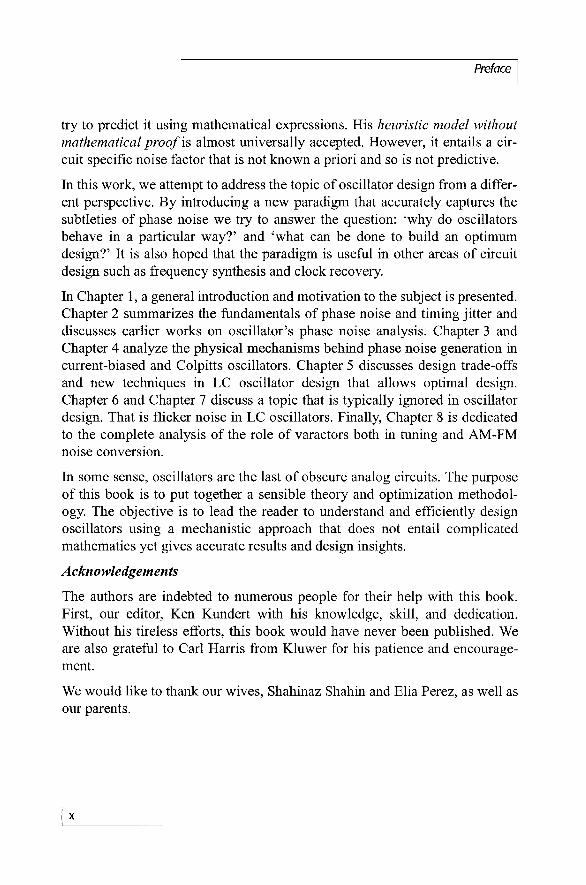
try to predict it using mathematical expressions. His heuristic model without mathematical proof is almost universally accepted. However, it entails a cir- cuit specific noise factor that is not known a priori and so is not predictive.

In this work, we attempt to address the topic of oscillator design from a differ- ent perspective. By introducing a new paradigm that accurately captures the subtleties of phase noise we try to answer the question: 'why do oscillators behave in a particular way?' and 'what can be done to build an optimum design?' It is also hoped that the paradigm is useful in other areas of circuit design such as frequency synthesis and clock recovery.

In Chapter 1, a general introduction and motivation to the subject is presented. Chapter 2 summarizes the fundamentals of phase noise and timing jitter and discusses earlier works on oscillator's phase noise analysis. Chapter 3 and Chapter 4 analyze the physical mechanisms behind phase noise generation in current-biased and Colpitts oscillators. Chapter 5 discusses design trade-offs and new techniques in LC oscillator design that allows optimal design. Chapter 6 and Chapter 7 discuss a topic that is typically ignored in oscillator design. That is flicker noise in LC oscillators. Finally, Chapter 8 is dedicated to the complete analysis of the role of varactors both in tuning and AM-FM noise conversion.

In some sense, oscillators are the last of obscure analog circuits. The purpose of this book is to put together a sensible theory and optimization methodol- ogy. The objective is to lead the reader to understand and efficiently design oscillators using a mechanistic approach that does not entail complicated mathematics yet gives accurate results and design insights.

Acknowledgements

The authors are indebted to numerous people for their help with this book. First, our editor, Ken Kundert with his knowledge, skill, and dedication. Without his tireless efforts, this book would have never been published. We are also grateful to Carl Harris from Kluwer for his patience and encourage- ment.

We would like to thank our wives, Shahinaz Shahin and Elia Perez, as well as our parents.

1 Preface

The authors would like to thank Linda Jaramillo, Henry and Sarah Rael. We would also like to thank Nikolaus Klemmer for multiple discussions and Wen Suter for encouragement.

Ernad Hegazi Jacob Rael Asad Abidi

August 12,2004

Basics of LC Oscillators 1

1 Introduction

Phase noise has been one of the most interesting yet poorly understood topics in circuit design. The challenge of predicting the amount of phase noise in a given circuit has been approached from a variety of angles, from using a "heu- ristic model without formal proof' [l] to simulation techniques that lead to accurate results [2][3]. Completing this book involved hours of computer sim- ulation, pages of algebra, translation of antiquated notation, and utilizing archeological-type efforts to unearth significant but otherwise forgotten papers.

With regard to this work, three major steps lead to the solution of this prob- lem. The first is Lesson's equation. All works on phase noise must reference Lesson's equation because it is simple, intuitive, and has withstood the test of time [I]. The second innovation was in the development of Cadence, Inc.3 SpectreRF simulation tool [2]. This tool accurately predicts phase noise and served as a test bench to validate all derived equations. Finally, Huang [4] showed it was possible to write out equations for phase noise explicitly. This work takes inspiration and elements from all these works and forms a model that is as intuitive as Leeson, as accurate as SpectreRF, and as rigorous as Huang.

2 The Mathematical Oscillator

The mathematical model of an ideal voltage-controlled oscillator starting at t = 0 is described by the following expression:

Chapter 1 Basics of LC Oscillators

where v, is the control voltage of the oscillator as a function of time. The cen- ter frequency of oscillation is o, and the instantaneous frequency of oscilla- tion is given by:

where Kv is the oscillator sensitivity and typically given in rad~seclvolt.

As can be seen from (I), the small signal model of an oscillator in frequency1 phase domain, with voltage as an input and phase as an output, functions as an integrator. The frequency of oscillation is directly proportional to the control voltage and the oscillator phase is the time-integral of frequency. Being a self- timed system, the oscillator lacks the ability to correct for its own phase. Imagine an oscillator running at some frequency with a constant bias applied to its control voltage line. Any disturbance on the control line will result in instantaneous frequency shift that integrates over the time the disturbance lasts. The resulting phase error will last indefinitely and can never be recov- ered even though the disturbance lasted for a short amount of time as shown in Figure 1.

FIGURE 1 Phase jitter accumulation.

, Time Grid

Control Voltage h

Time

1 3 Additive White Noise in LC Oscillato~s

3 Additive White Noise in LC Oscillators

An oscillation is fully characterized by its amplitude and phase. When white noise is added to an oscillation, noise corrupts both the amplitude and phase of oscillation. Assume a noise signal n(t) added to an oscillation v(t). It is cus- tomary to model noise as an infinite number of uncorrelated sinusoids sepa- rated by l Hz each. The sum of the oscillation signal at o, and a noise signal at frequency (I>, + con is given by:

where a, is the noise amplitude and (P, is a random phase. This equation can re-written as

The first three terms constitute an amplitude modulated carrier with the mod- ulating tones at w,. The last two terms together with the carrier, approximate a narrow band phase modulation signal. This means that a single sideband noise component added to the oscillator modulates both the amplitude and phase of the oscillation. The power of amplitude modulation sidebands is equal to the power of phase modulation sidebands.

In Chapter 2, we will rigorously define phase noise. For now, any noise that modulates the phase of oscillation is phase noise. Any noise that modulates the amplitude is considered amplitude noise and is unimportant in most prac- tical cases, except when it later converts to phase or frequency noise.

4 The Linear Oscillator

4.1 Warning

In this section, we develop a misleading analysis of oscillators based on linear system theory. Despite looking reasonable, we will show later why it is not accurate or even correct.

Chapter 1 Basics of LC Oscillators

4.2 Linear System Theory Applied to Oscillators

Oscillators are fundamentally nonlinear. In fact oscillator's nonlinearity is the reason for their "stable" amplitude. Yet linear models are often used to describe oscillatory behavior. This is acceptable when oscillation start-up conditions are pursued because oscillation at start-up is a small signal. How- ever, the periodically stable frequency can be far different from the small sig- nal "linear" prediction. Furthermore, a linear oscillator model cannot predict the oscillation amplitude. In fact, the assumption of linearity, leads to an un- determined amplitude. This is because in a linear system, if the input doubles, the output doubles. In an oscillator, this leads to an amplitude that is arbitrary P I . So what is a linear model good for?

1. It can yields a startup condition for oscillation, and

2. it gives a rough estimate of the frequency of oscillation.

FIGURE 2 Basic LC oscillator:

Consider the LC oscillator shown in Figure 2. If the oscillator loop is cut at any point, the gain around the loop is given by:

1 4 The Linear Odlator

For a sustained oscillation, Barkhausen criterion mandates that the gain around the loop is exactly unity and the phase shift around the loop is pre- cisely 360 degrees. This leads to the following:

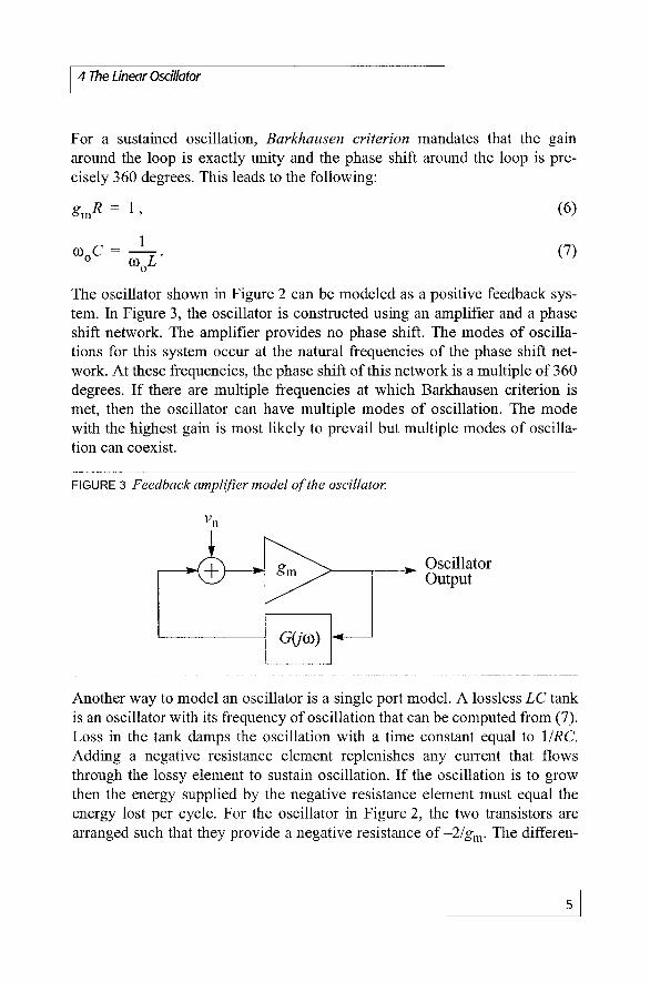
The oscillator shown in Figure 2 can be modeled as a positive feedback sys- tem. In Figure 3, the oscillator is constructed using an amplifier and a phase shift network. The amplifier provides no phase shift. The modes of oscilla- tions for this system occur at the natural frequencies of the phase shift net- work. At these frequencies, the phase shift of this network is a multiple of 360 degrees. If there are multiple frequencies at which Barkhausen criterion is met, then the oscillator can have multiple modes of oscillation. The mode with the highest gain is most likely to prevail but multiple modes of oscilla- tion can coexist.

FIGURE 3 Feedback amplEfier model o f the oscillator:

Another way to model an oscillator is a single port model. A lossless LC tank is an oscillator with its frequency of oscillation that can be computed from (7). Loss in the tank damps the oscillation with a time constant equal to 1IRC. Adding a negative resistance element replenishes any current that flows through the lossy element to sustain oscillation. If the oscillation is to grow then the energy supplied by the negative resistance element must equal the energy lost per cycle. For the oscillator in Figure 2, the two transistors are arranged such that they provide a negative resistance of -2/g,. The differen-

Chapter 1 Basics of LC Oscillators

tial resistance of the tank is 2R. Therefore, for a sustained oscillation, the neg- ative resistance should be equal to the positive resistance at all times. This leads back to (6). Redrawn in Figure 4, this circuit is known as the voltage- biased oscillator.

FIGURE 4 Basic LC oscillator (redrawn).

r̂

5 Linear Oscillator Noise Analysis Imagine an oscillator constructed using a parallel LC tank and a transconduc- tor in a positive feedback loop. The frequency of oscillation is of course given by (7). Note that the resonant frequency of the LC tank is the same as the oscillation frequency because both the resistor and the transconductor do not provide any extra phase shift as they carry no reactive current. The reader can readily prove that if the resistive loss is modeled in series with the inductor rather than it parallel, the oscillation frequency will be different from that given by (7).

Now let's consider the noise. Noise can come from two sources in this sys- tem: the resistor and the transconductor. Resistor noise is modeled by a white thermal noise current whose density is given by:

Noise in the transconductor is also modeled as a white noise current whose density is given by:

1 5 Linear Oscillator Noise Analysis

nL

i,(f 1 = 4kTg,J (9)

where y is the noise figure of the transconductor element.

The combined noise can be referred to the input of the transconductor as a white noise voltage given by:

Substituting from (6), the input referred noise voltage at the transconductor input is given by:

where F = 1 + y is the noise figure of the entire oscillator.

The tank impedance at a frequency 6o away from the resonance frequency can be approximated by

where Q is the tank quality factor.

Using basic feedback theory, it is trivial to prove that the closed-loop transfer function from the noise input to the oscillator output is given by:

In noise analysis, it is customary to represent noise by a sine wave in a 1 Hz bandwidth. Let's consider a noise component at a frequency do away fi-om the carrier (i.e. oscillation fundamental tone). Noise power at the output of the oscillator can be deduced using (1 1) and (13),

Chapter 1 Basics of LC Oscilato~~ 1

As shown earlier, additive noise shows as half amplitude noise and half phase noise. The noise-to-carrier ratio is obtained by dividing the output phase noise by the carrier power. We should also consider noise in the lower side band at o, + 6o. The single side band noise to carrier ratio is obtained by add- ing noise power at +6o and -60 resulting in the following expression:

This is the renowned Leeson's equation [I]. In the original paper it was given as a heuristic equation without formal prooj The preceding analysis is not part of the original paper that was based on measurements and observations. Many other researchers and design engineers derived, over the years, proofs similar to the one we derived here and ended up with one version or another of (1 5).

What's wrong with the above analysis? First, it is linear and time invariant. Therefore, no frequency translations of noise can occur. This means that low frequency noise, such as flicker noise, cannot create phase noise under the assumptions of this model. The only type of noise that can create phase noise in this model is noise originating around the oscillation frequency. Moreover, it has to have an equivalent amount of amplitude noise because it is in essence, additive noise. In any LC oscillator, this is not true. As we will show later, some elements contribute pure phase noise and no amplitude noise. Finally, linear analysis cannot predict the amplitude of oscillation. The ampli- tude limiting mechanism is fundamentally nonlinear and cannot be captured in the context of a linear time-invariant analysis.

6 How Is This Book Different?

In the following chapters we will show in detail why the derivation in Section 4 is wrong. We will show how to use circuit theory to derive an accu- rate model for phase noise in electrical oscillators. We will describe what we call a mechanistic model that captures the dominant nonlinearities in an oscil- lator and provides a closed form expression for phase noise. No fudge factors utilized!

1 References

Concepts from nonlinear circuit theory are sometimes utilized yet we tried to keep that to the minimum necessary.

By doing so, this book provides deep insight into the operation of oscillators and provides simple procedures for designing high-purity oscillators. We are answering the seldom tackled questions: 'why does the oscillator behave that way?' and 'how is an optimal oscillator designed?'

References

D. B. Leeson, "A simple model of feedback oscillator noise spectrum," Pro- ceedings of the IEEE, vol. 54, pp. 329-330, 1966.

K. S. Kundert, "Introduction to RF simulation and its application," IEEE J. Solid-state Circuits, pp. 1298-3 19, 1999. Also available from www. designers- guide. com/Analysis.

A. Hajimiri and T. H. Lee, "A general theory of phase noise in electrical oscilla- tors," IEEE Journal of Solid-state Circuits, vol. 33, pp. 179-94, 1998.

Q. Huang, "On the exact design of RF oscillators," Proceedings of the IEEE 1998 Custom Integrated Circuits Conference, 1 99 8.

Thomas Lee, Radio Frequency Integrated Circuits, Cambridge University Press, 1998.

Oscillator Purity

A sinusoidal oscillation is described completely by its amplitude and fre- quency. The purity of the oscillation pertains typically to only the frequency or period of oscillation. This is because an oscillator is typically used to syn- chronize events in time. This applies to wireless transceivers as well as digital circuits. The amplitude of oscillation, once above a threshold value, is typi- cally irrelevant as long as it can generate an action (event) on the subsequent circuit block. An oscillation that is perfectly pure has a constant period of rep- etition. In frequency domain, the perfect repetition translates into a single tone, for a sinusoidal oscillation anyway.

Historically, observing periodicity in time predates the observation of spectral purity for obvious reasons. Ancient Egyptians noted that Sirius rises to its place besides the sun exactly every 365 days. They divided the year into twelve 30-day months and a short 5 day month that was called the "little month". Their calendar is still used today by peasants in the countryside of Egypt, side-by-side with the Gregorian calendar, as it fits perfectly the Egyp- tian climate and the flooding of the Nile. Their calendar was the basis of the modern calendar we use today. The Babylonians of today's Iraq used a lunar calendar that follows the periodicity of the moon, a cycle of 29 to 30 days. They are the ones who divided the day into smaller units that relate to their base-60 numeral system. Around the 1 6 ~ ~ century, in the era of great expedi- tions, there was a great need for accurate clocks for navigation. Determining longitude accurately was not possible without a tool that can tell time with

Chapter 2 Oscillator Purify Fundamentals

great accuracy [I]. Galileo sketched out the concept of the first pendulum- based clock. It was Harrison who first implemented a clock that can tell time within one second of error per day [I]. Various designs of mechanical move- ments were implemented over the centuries that followed and are perfected today in Swiss mechanical watches. The 1920s witnessed the first quartz clock that enabled much higher frequencylperiod stability. Later, this fueled the clock industry in Japan. For more accurate time bases, the atomic clock is used as a calibration source. The search for the most accurate clock is in essence the search for a high long-term stability signal source. The question of noise in signal sources was not of concern until World War 11. Only then was the study of noise in the oscillator's phase was born. In essence, phase noise relates to the short-term stability of the oscillator's period, frequency, or phase.

Signal purity measures can be divided into two main categories: deterministic and stochastic. Deterministic impurity comes from spurious signals that show in the signal spectrum as delta-Dirac impulses, known as spurs at a fixed fre- quency offset from the main tone. Stochastic impurity arises from stochastic variation of signal phase and are manifested in noise skirts around the funda- mental frequency. Another way of quantifying stochastic purity is by looking at the signal in time domain where stochastic perturbations are manifested as perturbations in the zero crossings of the sinusoidal waveform. For practical RF receiver design purposes, amplitude perturbations are typically of little concern because mixers are not sensitive to them. In transmitters, however, the situation is somewhat different. Amplitude noise would interfere with neighboring channels just as phase or frequency noise does if it spills out of its allotted bandwidth.

In this chapter we briefly describe the basic concepts of signal purity both in time and frequency domains. The reader who is familiar with these concepts can skip this chapter and advance to chapter 3.

2 Timing Jitter A pure oscillation repeats in time precisely every T seconds, where T is called the oscillation period. In other words, if we set a particular threshold voltage level, the oscillation waveform will cross this threshold in a given direction precisely every T seconds. In the presence of noise, the points in time where

1 2 Timing Jitter

the oscillation waveform crosses this threshold are dithered around their ideal noiseless locations. In statistical terms, the oscillation waveform is a random process described by:

where $, is a stochastic process that produces a random phase fluctuation.

Consider now different realizations of this random process, i.e. different pos- sible waveforms that fulfill (1). Such realizations are shown in Figure 1. The first waveform is an ideal noiseless oscillation. The other two waveforms are sample realizations for different values of $,(t) that have the same statistical properties. The threshold is held at the V(t) = 0. As shown, each of the two realizations rises through the threshold at random time points around the ideal waveform crossing points. The difference in the crossing time between the ideal waveform and the various realizations is a random process denoted by Aji. It is assumed that all of the realizations of the random process V(@,, t ) start from the same zero initial phase. The subscript j denoted the realization number whereas the subscript i denotes the count of the threshold crossing starting from the initial phase at i = 0.

At any particular zero crossing i, the difference in crossing times is a random variable that has some particular mean and variance. Consider the zeroth crossing, i.e. at the initial point; all values of Ajo are equal to zero because all realizations of V(8, t ) start at the same initial phase. Therefore, the random variable Ajo has zero mean and zero variance. In other words, the probability distribution of Ajo is an impulse,

where 6 is the delta-Dirac impulse.

Now comes into play, the most characteristic property of oscillators; they are autonomous circuits. The phase of the oscillator is determined only from within. This means that the ending point of cycle 1 is the starting point of cycle 2 and the phase error incurred in cycle 1 is carried over without correc- tion to cycles 2 and 3, .... indefinitely. This is manifested in the basic mathe- matical model of oscillators shown in Chapter 1; the oscillator is a phase integrator. This means that if we try to evaluate the statistical properties of A at the end of cycle m (Ai,), we are actually looking at the accumulation (inte-