UNLV Theses, Dissertations, Professional Papers, and Capstones

May 2018

The Design, Modeling, and Optimization of a Biomimetic Soft The Design, Modeling, and Optimization of a Biomimetic Soft

Robot for Fluid Pumping and Thrust Generation Using Robot for Fluid Pumping and Thrust Generation Using

Electroactive Polymer Actuators Electroactive Polymer Actuators

Zakai Jedidiah Olsen

Follow this and additional works at: https://digitalscholarship.unlv.edu/thesesdissertations

Part of the Mechanical Engineering Commons

Repository Citation Repository Citation Olsen, Zakai Jedidiah, "The Design, Modeling, and Optimization of a Biomimetic Soft Robot for Fluid Pumping and Thrust Generation Using Electroactive Polymer Actuators" (2018). UNLV Theses, Dissertations, Professional Papers, and Capstones. 3301. http://dx.doi.org/10.34917/13568638

This Thesis is protected by copyright and/or related rights. It has been brought to you by Digital Scholarship@UNLV with permission from the rights-holder(s). You are free to use this Thesis in any way that is permitted by the copyright and related rights legislation that applies to your use. For other uses you need to obtain permission from the rights-holder(s) directly, unless additional rights are indicated by a Creative Commons license in the record and/or on the work itself. This Thesis has been accepted for inclusion in UNLV Theses, Dissertations, Professional Papers, and Capstones by an authorized administrator of Digital Scholarship@UNLV. For more information, please contact digitalscholarship@unlv.edu.

THE DESIGN, MODELING, AND OPTIMIZATION OF A BIOMIMETIC SOFT ROBOT

FOR FLUID PUMPING AND THRUST GENERATION USING ELECTROACTIVE

POLYMER ACTUATORS

By

Zakai J. Olsen

Bachelor of Science in Engineering – Mechanical Engineering University of Nevada, Las Vegas

2016

A thesis submitted in partial fulfillment of the requirements for the

Master of Science in Engineering – Mechanical Engineering

Department of Mechanical Engineering Howard R. Hughes College of Engineering

The Graduate College

University of Nevada, Las Vegas May 2018

ii

Thesis Approval

The Graduate College

The University of Nevada, Las Vegas

April 13, 2018

This thesis prepared by

Zakai J. Olsen

entitled

The Design, Modeling, and Optimization of a Biomimetic Soft Robot for Fluid Pumping

and Thrust Generation Using Electroactive Polymer Actuators

is approved in partial fulfillment of the requirements for the degree of

Master of Science in Engineering – Mechanical Engineering

Department of Mechanical Engineering

Kwang Kim, Ph.D. Kathryn Hausbeck Korgan, Ph.D. Examination Committee Chair Graduate College Interim Dean

Mohamed Trabia, Ph.D. Examination Committee Member

Woosoon Yim, Ph.D. Examination Committee Member

Rebecca Martin, Ph.D. Graduate College Faculty Representative

iii

Abstract

Nature is a constant source of inspiration for engineers and scientists through its simple,

effective, and elegant solutions to many complex problems. Smart materials and soft robotics

have been seen to be particularly well suited for developing biomimetic devices and are active

fields of research. In this study, the design, modeling, and optimization of a new biomimetic soft

robot is described. Preliminary work was made in the modeling of a biomimetic robot based on

the locomotion and kinematics of jellyfish. Modifications were made to the governing equations

for jellyfish locomotion that accounted for geometric differences between biology and the

robotic design. Particularly, the capability of the model to account for the mass and geometry of

the robot design. A simple geometrically defined model is developed and used to show the

feasibility of a proposed biomimetic robot. With the concept verified, a more robust physics-

based model is developed. In this model, linear beam theory is coupled to an equivalent circuit

model to actuate the robot with ionic polymer-metal composite (IPMC) actuators. The circuit

model is verified using a robust, Multiphysics finite element model of the IPMC actuator. The

newly created physics-based model of the soft robot is compared to that of the geometric model

as well as biological jellyfish swimming to highlight its improved efficiency. The design is then

optimized using a sequential quadratic programming algorithm for nonlinear multivariable

optimization. Standard deviations of the optimized values are used to verify their accuracy, and

the propulsion efficiency of the unoptimized and optimized model are compared to verify the

improvement in efficiency and overall performance. Scale effects on the optimal design are also

examined as an initial form of dimensional analysis. The optimized design shows clear

improvement over the unoptimized counterpart, and the modularity of the modeling approach

allows for more complex models that include nonlinearities to be easily added.

iv

Acknowledgements

I would like to thank my advisor, Dr. Kwang Kim, for his immense support and advice

throughout my undergraduate and graduate studies. His mentorship, teaching, financial support,

research guidance, and amazing travel opportunities given to me have greatly shaped my career

as an engineer and researcher. I am profoundly grateful for Dr. Kim’s generosity and interest

invested in these many areas of my life, all of which have helped lead me to graduating at this

time.

I would also like to thank committee members, Dr. Mohamed Trabia, Dr. Woosoon Yim,

and Dr. Rebecca Martin for their teaching and advice during my career at UNLV. I truly

appreciate their time and interest spent on my studies and development as a researcher.

All of the faculty and staff who have had such a positive impact on me throughout my

time at UNLV are very much appreciated and my sincere thanks go to each of them. The

incredible professors I have studied under have given me the education necessary to pursue a

graduate career, and beyond. I would like to specifically thank Joan Conway for all her

incredible assistance, encouragement, and support. All my colleagues in the AMSL lab who

helped me throughout my graduate studies are well-deserving of my thanks. Their advice and

support are greatly appreciated, equally as much as their friendship. I also thank the National

Science Foundation PIRE program and the Nevada NASA Space Grant Consortium for the

funding and support for my graduate research.

Finally, an acknowledgement of warmhearted gratitude for my friends and family. Their

continual support of my academic and professional endeavors has helped me stay focused and

level-headed. I particularly give special thanks to my younger brother, Luke Olsen, for always

being there to give his advice and perspective whenever I needed it.

v

Table of Contents

Abstract .......................................................................................................................................... iii

Acknowledgements ........................................................................................................................ iv

List of Tables ................................................................................................................................ vii

List of Figures .............................................................................................................................. viii

Nomenclature ................................................................................................................................. xi

Chapter 1. Introduction ................................................................................................................... 1

Chapter 2. Biological Inspiration .................................................................................................... 3

2.1. Kinematics of Swimming Jellyfish .................................................................................... 3

2.1.1. Derivation of Governing Equations .......................................................................... 4

2.1.2. Modeling of Jellyfish Locomotion............................................................................ 8

2.2. Design Principle of a Biomimetic Jellyfish ..................................................................... 12

Chapter 3. Electromechanical Modeling of Ionic Polymer-Metal Composite Actuators ............. 14

3.1. Physics-Based Modeling .................................................................................................. 14

3.1.1. Governing Partial Differential Equations ............................................................... 15

3.1.2. Multi-Physics Modeling in COMSOL .................................................................... 18

3.2. Equivalent Circuit Modeling............................................................................................ 26

3.2.1. RCW Circuit Model ................................................................................................ 27

3.3. Comparison and Utility of Modeling Approaches ........................................................... 30

Chapter 4. Modeling of a Biomimetic Soft Robot ........................................................................ 32

4.1. Governing Equation and Model Inputs ............................................................................ 32

4.2. Geometry Based Modeling .............................................................................................. 35

4.2.1. Description of Robot Body as Geometric Surface .................................................. 35

vi

4.2.2. Derivation of Model Parameters ............................................................................. 36

4.2.3. Comparison to Biological Jellyfish ......................................................................... 39

4.3. Physics-Based Modeling .................................................................................................. 43

4.3.1. Beam Theory Approach .......................................................................................... 44

4.3.2. Derivation of Model Parameters ............................................................................. 53

4.3.3. Addition of IPMC Electromechanical Effects ........................................................ 56

4.3.4. Evaluation and Comparison to Previous Model ..................................................... 58

Chapter 5. Design Optimization ................................................................................................... 64

5.1. Sequential Quadratic Programming Optimization ........................................................... 64

5.1.1. Selection of Design Variables ................................................................................. 64

5.1.2. Optimization of Design Variables .......................................................................... 69

5.2. Comparison of Unoptimized and Optimized Design ....................................................... 73

5.3. Scale Effects on Optimal Parameter Values .................................................................... 76

5.4. Discussion ........................................................................................................................ 79

Chapter 6. Conclusion ................................................................................................................... 81

Chapter 7. Future Work ................................................................................................................ 84

7.1. Fabrication of Prototype .................................................................................................. 84

7.2. Structure of Future Experimental Study .......................................................................... 87

7.3. Additions to Physics-Based Model .................................................................................. 88

Appendix A: Additional Figures of COMSOL Domains and Mesh............................................. 89

Appendix B: Coefficients for Volume and Cross-Sectional Area in Physics-Based Model ........ 92

Bibliography ................................................................................................................................. 94

Curriculum Vitae ........................................................................................................................ 105

vii

List of Tables

Table 3.1 Model parameters for 2D vs 1D PNP Comparison....................................................... 20

Table 3.2 Metrics for 1D vs 2D PNP Comparison ....................................................................... 22

Table 3.3 Metrics for 1D vs Refined 1D PNP Comparison .......................................................... 24

Table 3.4 Parameters and Dimensions of IPMC Used for Experimental Comparison ................. 26

Table 3.5 Parameter Values for Equivalent Circuit Model ........................................................... 29

Table 4.1 Direction Cosine Angles for Inlet and Outlet During Different Swimming Modes ..... 39

Table 4.2 Beam Geometry and Loading for COMSOL Comparison ........................................... 51

Table 4.3 Physics-Based Model Comparison Parameters ............................................................ 60

Table 5.1 Simulation Parameters for IPMC Length Optimization ............................................... 66

Table 5.2 Simulation Parameters for Pairwise Optimization........................................................ 67

Table 5.3 Parameter Values for Unoptimized and Expected Optimal Designs ............................ 69

Table 5.4 Parameters for SQP Optimization of Design Variables................................................ 71

Table 5.5 Results of SQP Optimization ........................................................................................ 73

Table 5.6 Propulsion Efficiency for Unoptimized and Optimized Models .................................. 75

Table 5.7 Results of Optimization with Scaled Shell Radius ....................................................... 77

viii

List of Figures

Figure 2.1 Illustration of Jet Propulsion Mechanism Found in Biological Jellyfish ................... 4

Figure 2.2 Illustration of Jellyfish Body Structure ...................................................................... 6

Figure 2.3 Free Body Diagram of Swimming Jellyfish .............................................................. 8

Figure 2.4 Position, Velocity, and Acceleration of Biological Jellyfish ................................... 12

Figure 2.5 Illustrative Cross-Section of Proposed Soft Robot Design ...................................... 13

Figure 3.1 Cantilever IPMC Diagram for COMSOL Multiphysics Modeling ......................... 19

Figure 3.2 COMSOL Domain for 1D PNP FEM ...................................................................... 20

Figure 3.3 Domain for 2D Solid Mechanics in COMSOL........................................................ 21

Figure 3.4 Comparison of 1D and 2D PNP Models .................................................................. 22

Figure 3.5 Differences in 1D Domain Structures Used in COMSOL ....................................... 23

Figure 3.6 Comparison of 1D and Refined 1D PNP Models .................................................... 24

Figure 3.7 Unconstrained IPMC Deformation Under External Stress Loading ........................ 25

Figure 3.8 Comparison Between Refined 1D COMSOL Model and Experimental Data ........ 26

Figure 3.9 Circuit Diagram Used for Equivalent Circuit IPMC Model .................................... 27

Figure 3.10 Comparison Between RCW Circuit Model and Experimental Data ....................... 30

Figure 3.11 Comparison of FEM, Equivalent Circuit, and Experimental IPMC Deflection ...... 31

Figure 4.1 Illustration of Direction Cosine for Inlet and Outlet Valves.................................... 34

Figure 4.2 Representative Waveforms Generated with Fourier Series Square Wave ............... 35

Figure 4.3 Geometric Description of Robot Body as an Ellipsoid ............................................ 36

Figure 4.4 Drag Coefficient as a Function of Reynold’s Number ............................................ 39

Figure 4.5 Input Half-Axis Dimension for Geometric Model, 1000th Partial Sum Input ......... 40

Figure 4.6 Simulation of Geometric Model with Various Inputs and Swimming Modes ........ 42

ix

Figure 4.7 Thrust Profile for Geometric Model in Both Swimming Modes ............................. 43

Figure 4.8 Diagram of Physics-Based Description of Robot Body .......................................... 44

Figure 4.9 Illustrative Cross-Section of Proposed Physics-Based Model ................................. 45

Figure 4.10 Comparison of Beam Theory to FEM Implementation ........................................... 51

Figure 4.11 Error of Straight Beam Assumption ........................................................................ 52

Figure 4.12 RCW Model Charge Response for Fourier Series Input ......................................... 58

Figure 4.13 Comparison of Physics-Based Model to Geometric and Jellyfish Models .............. 59

Figure 4.14 Thrust Profile for Physics-Based Model .................................................................. 61

Figure 4.15 Mass Flux for Physics-Based Model ....................................................................... 61

Figure 4.16 Velocity Profiles for Fluid Pump Operation ............................................................ 63

Figure 5.1 Distance vs IPMC Length ........................................................................................ 65

Figure 5.2 Surface Plot of Distance vs Length and Contraction Time...................................... 67

Figure 5.3 Surface Plot of Distance vs Length and Time Ratio ................................................ 68

Figure 5.4 Surface Plot of Distance vs Time Ratio and Contraction Time ............................... 68

Figure 5.5 Probability Density Function: IPMC Length ........................................................... 72

Figure 5.6 Probability Density Function: Time Ratio ............................................................... 72

Figure 5.7 Probability Density Function: Contraction Time ..................................................... 73

Figure 5.8 Comparison of Unoptimized and Optimized Models: Distance Traveled ............... 74

Figure 5.9 Velocity Profiles for Efficiency Calculation............................................................ 75

Figure 5.10 Optimized IPMC Length Versus Radius of Shell .................................................... 77

Figure 5.11 Optimized Time Ratio Versus Radius of Shell ........................................................ 78

Figure 5.12 Optimized Contraction Time Versus Radius of Shell .............................................. 78

Figure 7.1 Engineering Sketch of Prototype Mold Design ....................................................... 84

x

Figure 7.2 Second Mold Design CAD Image ........................................................................... 85

Figure 7.3 First 3D Printed Mold .............................................................................................. 86

Figure 7.4 Second 3D Printed Mold .......................................................................................... 86

Figure 7.5 Current Status of Elastomer Prototype Body ........................................................... 87

Figure A.1 Finite Element Mesh for 2D PNP Domain .............................................................. 89

Figure A.2 Enhanced View of Figure A.1 ................................................................................. 89

Figure A.3 Finite Element Mesh of 2D Solid Mechanics Domain ............................................ 89

Figure A.4 Enhanced View of Figure A.3 ................................................................................. 90

Figure A.5 Finite Element Mesh of 1D PNP Domain................................................................ 90

Figure A.6 Enhanced View of Figure A.5, Electrode-Polymer Interface .................................. 90

Figure A.7 Enhanced View of Figure A.5, Membrane-Membrane Interface ............................ 90

Figure A.8 Finite Element Mesh of 2D Solid Mechanics Domain for 1D PNP Modeling ........ 91

Figure A.9 Enhanced View of Figure A.8 ................................................................................. 91

xi

Nomenclature

𝐴𝐴𝑣𝑣 Velar / valve aperture area (m2) 𝛼𝛼ℎ Hydrofilicity coefficient

(N-m/mol) 𝛼𝛼𝐴𝐴𝐴𝐴 Added mass coefficient 𝛼𝛼𝑅𝑅𝑅𝑅𝑅𝑅 Hydrofilicity coefficient for

circuit model (N/m-C) 𝛼𝛼𝑐𝑐 Hydrofilicity coefficient in

COMSOL (N/C) 𝛼𝛼 Starting polar angle 𝛽𝛽ℎ Hydrofilicity coefficient

(N-m4/mol2) 𝛽𝛽 Ending polar angle 𝐶𝐶𝑑𝑑 Drag coefficient 𝑐𝑐0 Anion concentraction (mol/m3) 𝐶𝐶 Stiffness tensor (Pa) 𝑐𝑐 Cation concentration (mol/m3) 𝐷𝐷𝑒𝑒 Electric displacement (C/m2) 𝐷𝐷𝑓𝑓𝑓𝑓𝑓𝑓𝑐𝑐𝑒𝑒 Drag force of jellyfish / robot

(N) 𝛿𝛿𝑖𝑖 Perturbation of ith SQP variable 𝛿𝛿𝑡𝑡 Time ratio 𝐷𝐷 Cation diffusivity (m2/s) 𝑑𝑑𝑑𝑑 Volume change for jellyfish

swimming model (m3) 𝐸𝐸�⃗ Electric field strength (N/C) 𝜀𝜀0 Dielectric constant in vacuum

(F/m) 𝜀𝜀𝑑𝑑 Strain tensor 𝜀𝜀𝑓𝑓 Relative dielectric constant 𝜂𝜂𝑝𝑝𝑓𝑓𝑓𝑓𝑝𝑝 Propulsion efficiency 𝜖𝜖𝐿𝐿 Minimum allowable passive

material (m) 𝐸𝐸 Young’s modulus (Pa) 𝜀𝜀 Absolute dielectric constant

(F/m) 𝜖𝜖 Axial strain 𝐹𝐹𝑏𝑏 Body forces (N/m3) 𝐹𝐹𝑖𝑖𝑖𝑖𝑒𝑒𝑓𝑓𝑡𝑡𝑖𝑖𝑖𝑖 Inertial force (N) 𝐺𝐺𝑝𝑝 Gauss-Legendre point 𝐺𝐺𝑤𝑤 Gauss-Legendre weight

𝐺𝐺 Acceleration reaction (N) ℎ Bell height (m) ℎ𝑡𝑡 Integrator time step (s) 𝐼𝐼 Moment of inertia (m4) 𝐽𝐽 Cation flux (mol/m3-s) 𝜅𝜅 Bending strain (1/m) 𝐿𝐿𝑐𝑐 Characteristic length (m) 𝑚𝑚 Mass of jellyfish / robot (kg) 𝜇𝜇 Cation mobility (s-mol/kg) 𝑁𝑁𝑤𝑤 Number of shape functions 𝑵𝑵𝒔𝒔 Vector of shape functions 𝑵𝑵𝜻𝜻 Vector of nondimensional shape

functions 𝜈𝜈 Kinematic viscosity of water

(m2/s) 𝑂𝑂𝐺𝐺 Order of gauss quadrature 𝑃𝑃𝑤𝑤 Transverse loading (N/m) 𝜙𝜙 Electric potential (V) 𝑄𝑄 Charge in IPMC (C) 𝜌𝜌𝑤𝑤 Density of water (kg/m2) 𝜌𝜌𝑐𝑐 Charge density (C/m3) 𝜌𝜌𝑚𝑚 Material density (kg/m3) 𝑅𝑅𝑅𝑅 Reynold’s number 𝑟𝑟 Instantaneous bell radius (m) 𝜌𝜌 Radius of curvature (m) 𝑆𝑆0 Initial cross-sectional area (m2) 𝑆𝑆𝐴𝐴 Cross-sectional area w.r.t flow

(m2) 𝜎𝜎𝑒𝑒𝑒𝑒𝑡𝑡 External stress (Pa) 𝜎𝜎 Stress tensor (Pa) 𝑡𝑡𝑐𝑐 Contraction time (s) 𝑡𝑡𝑚𝑚 Time since last contraction cycle

start (s) 𝑡𝑡𝑓𝑓 Relaxation time (s) 𝜃𝜃𝑠𝑠 Polar angle of beam (rad) 𝑇𝑇 Thrust force of jellyfish / robot

(N) 𝑡𝑡 Time (s) 𝑢𝑢𝑒𝑒 Velocity of exchanged fluid

(m/s)

xii

𝑢𝑢�⃗ Material displacement field (m) 𝑢𝑢𝑒𝑒 Deflection along x-axis (m) 𝑢𝑢𝑦𝑦 Deflection along y-axis (m) 𝑢𝑢 Swimming velocity (m/s) 𝑑𝑑𝑓𝑓 Total volume of fluid (m3) 𝑑𝑑𝑖𝑖 Internal volume 𝑣𝑣𝑒𝑒 Ejected fluid velocity (m/s) 𝑣𝑣 Axial deflection (m) 𝑤𝑤 Transverse deflection (m) 𝑤𝑤� Trial displacemnt (m) 𝑤𝑤� Galerkin coefficient 𝑤𝑤�� Modified Galerkin coefficient 𝒘𝒘� Vector of coefficients 𝑋𝑋𝑖𝑖,0 Initial value of ith SQP variable 𝑥𝑥𝑖𝑖 Nominal value of ith SQP

variable 𝑍𝑍𝑅𝑅𝑖𝑖𝑝𝑝 Capacitive impedance (1/F) 𝑍𝑍𝑅𝑅 Resistive impedance (Ohm) 𝑍𝑍𝑅𝑅𝑖𝑖𝑓𝑓𝑏𝑏𝑊𝑊𝑓𝑓𝑊𝑊 Warburg ipmedance (1/Ohm-s2) 𝑧𝑧 Charge number 𝜁𝜁 Nondimensional axial

coordiante

1

Chapter 1. Introduction

Over the last 25 years, electroactive polymers (EAP) have emerged and grown into a vast

and diverse field of research, with numerous potential applications in soft robotics and smart

materials. Due to their similar behavior to biological muscle, these materials are commonly

referred to as artificial muscles [1]. O’Halloran et al give an overview of EAP technology in [2],

but the basic operation of these materials is a transduction of electrical stimuli into mechanical

deformation. Most EAP materials have the capability of both electromechanical transduction,

where they can act as actuators [3–5], as well as mechanoelectrical transduction, where they

work as sensors [6–9]. This duality lies in the fundamentals of the electrochemical nature that

governs both transduction modes, and is explored throughout literature [10–13]. The class of

EAP includes materials such as dielectric elastomers, ferroelectric polymers, ionic polymer gels,

and many more [2].

In this work the focus is placed on the ionic polymer-metal composite (IPMC). This

material consists of an ionic polymer, typically Nafion® or Aquivion® [4,14], that is composited

between two electrodes, most commonly platinum or gold. While there are a few fabrication

methods for such materials, typically the electrodes are plated to an activated polymer membrane

through an electroless process [15]. IPMC actuators have a unique characteristic in that they

exhibit large mechanical deformations in response to a relatively low voltage [1,11,14,16,17],

making them attractive for compact, low power soft robotics.

IPMCs achieve their electromechanical transduction due to free moving cations within

the polymer that are hydrated with water molecules. Under an applied electric potential to the

electrodes, these hydrated cations migrate to the cathode and cause swelling at the polymer-

electrode interface, which in turn bends the IPMC towards the anode. Due to the similarities of

2

EAP to biological muscle, biology inspires many soft robotic designs seen in literature. This

gives rise to an entire field of soft robotics, namely, biomimetic soft robotics [5,18].

The IPMCs ability to actuate in water [19–22] has focused the soft robotics development

heavily on aquatic animals. The biomimetic applications of IPMCs range from small scale

biological structures such as cilia [23] all the way up to full size robots [24]. Fabrication of fin-

like actuators has been demonstrated in [15,25,26], while the authors in [27–32] all worked on

developing small fish-like robots. Manta ray robots are seen in the works of [33,34], and a tiny

dolphin robot is found in [35]. As will be elaborated on later, the jellyfish is of interest for this

research. Many others have developed biomimetic jellyfish robots, using EAPs as well as

traditional robotic actuators. A few of these designs can be found in [36–42].

The jellyfish has been the focus of many researchers in the biology and engineering field,

with varying interests in its swimming mechanism. As will be discussed in the next chapter, the

jellyfish utilizes what is known as a jet propulsion method of locomotion. This has been

extensively explored throughout literature from hydrodynamic, kinematic, and geometric

perspectives. The interest here is to examine the behavior of the swimming jellyfish and develop

a new biomimetic soft robot that builds on the basic mechanisms used in biology for locomotion

and address any observed limitations.

3

Chapter 2. Biological Inspiration

2.1. Kinematics of Swimming Jellyfish

The work of [43] gives a great overview on biological and bioinspired forms, and has a

wide breadth of information on the propulsion mechanisms used in nature by aquatic animals.

There, the mechanism of jet propulsion is described as a method for fish locomotion. Jet

propulsion is broken into three categories, bell constriction, mantel constriction, and shell

compression. The jellyfish, as noted in the aforementioned work, mainly utilizes the bell

constriction form of jet propulsion.

This swimming behavior is characterized by the movement of a flexible bell, and

propulsion is generated during alternating contraction and relaxation phases of the bell muscles,

ejecting or refilling water into the volume of the bell. Two forms of bell constriction are

available to jellyfish, depending on their geometry. Namely, jet and rowing propulsion, which

are similar in the muscles activated during swimming, but differentiated by size of the muscle

necessary to achieve each. The jet method of propulsion is of interest in this work, and it will be

assumed from here onward that when referring to jellyfish swimming that jet propulsion will be

the mechanism that is used. An illustrative graphic of the bell deformation that occurs during the

contraction and relaxation phases is provided in Figure 2.1.

Numerous studies have been conducted into the self-propulsion of aquatic animals.

Specifically, Lauder et al. researched the use of bio-robotic models and how they may provide

insight into the hydrodynamics and kinematics of aquatic propulsion, Lu et al. investigated the

hydrodynamics of fish-like swimming through the use of numerical and experimental studies,

and Triantafyllou et al. worked on the optimal thrust generated via jet-like flows from oscillating

4

foils similar to that of fish fins [44–46]. More in line with the work presented here, the jet

propulsion of aquatic animals such as the jellyfish has been studied in [47–49].

The jellyfish itself has been the center of numerous studies involving a wide range of

topics, such as the flow patterns during swimming, bell deformation kinematics, dynamics and

structure, and the hydrodynamic effects of the biological structure and locomotion of the animal.

These topics can be found throughout literature in [50–57]. Of particular interest is the work

found in [51,58,59] where dynamic equations of motion (EoM) can be found that can be used to

model the biological jet propulsion of jellyfish. These will be used and modified later in order to

simulate the swimming of a proposed biomimetic soft robot.

Figure 2.1 Illustration of Jet Propulsion Mechanism Found in Biological Jellyfish In between contraction and relaxation phases the fluid contained within the body of the jellyfish is exchanged with the surrounding fluid and the momentum exchanged in this process results in a net-positive thrust over the duration of a complete swimming cycle.

2.1.1. Derivation of Governing Equations

The jet propulsion mechanism of the jellyfish as studied in [58] follows a simple dynamic

EoM that can be used to simulate the swimming behavior of biological jellyfish. This also

provides a source point for modeling jellyfish-like robotics, which will be demonstrated later in

Chapter 4.1. Here, the governing equation is re-derived from [58] and analyzed to visualize how

Contraction

Relaxation

5

biological jellyfish swim, as well as give rise to the inspiration that leads to the development of

the soft robot design presented later in this chapter.

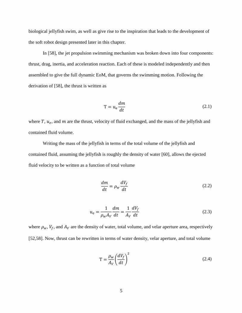
In [58], the jet propulsion swimming mechanism was broken down into four components:

thrust, drag, inertia, and acceleration reaction. Each of these is modeled independently and then

assembled to give the full dynamic EoM, that governs the swimming motion. Following the

derivation of [58], the thrust is written as

T = ue𝑑𝑑𝑚𝑚𝑑𝑑𝑡𝑡

(2.1)

where 𝑇𝑇, 𝑢𝑢𝑒𝑒, and 𝑚𝑚 are the thrust, velocity of fluid exchanged, and the mass of the jellyfish and

contained fluid volume.

Writing the mass of the jellyfish in terms of the total volume of the jellyfish and

contained fluid, assuming the jellyfish is roughly the density of water [60], allows the ejected

fluid velocity to be written as a function of total volume

𝑑𝑑𝑚𝑚𝑑𝑑𝑡𝑡

= 𝜌𝜌𝑤𝑤𝑑𝑑𝑑𝑑𝑓𝑓𝑑𝑑𝑡𝑡

(2.2)

ue =1

𝜌𝜌𝑤𝑤𝐴𝐴𝑉𝑉𝑑𝑑𝑚𝑚𝑑𝑑𝑡𝑡

=1𝐴𝐴𝑉𝑉

𝑑𝑑𝑑𝑑𝑓𝑓𝑑𝑑𝑡𝑡

(2.3)

where 𝜌𝜌𝑤𝑤, 𝑑𝑑𝑓𝑓, and 𝐴𝐴𝑉𝑉 are the density of water, total volume, and velar aperture area, respectively

[52,58]. Now, thrust can be rewritten in terms of water density, velar aperture, and total volume

T =𝜌𝜌𝑤𝑤𝐴𝐴𝑉𝑉

�𝑑𝑑𝑑𝑑𝑓𝑓𝑑𝑑𝑡𝑡

�2

(2.4)

6

The drag component in the EoM is governed by the standard drag equation, given as

Dforce =12

Cd𝜌𝜌𝑤𝑤𝑆𝑆𝐴𝐴𝑢𝑢2 (2.5)

where 𝐷𝐷 is the drag force, 𝐶𝐶𝑑𝑑 is the drag coefficient, 𝑆𝑆𝐴𝐴 is the cross-sectional area with respect to

the swimming direction, and 𝑢𝑢 is the swimming speed of the jellyfish. Both the drag coefficient

and cross-sectional area change as the jellyfish body deforms during swimming. To obtain the

cross-sectional area, the truncated bell shape is used to derive the following expression for area

as a function of volume

SA = 𝑆𝑆0 +32ℎ

𝑑𝑑𝑑𝑑𝑓𝑓𝑑𝑑𝑡𝑡

𝑡𝑡 (2.6)

with 𝑆𝑆0 being the initial cross-sectional area and ℎ the height of the bell geometry at the start of a

contraction phase. The structure of this truncated bell shape is shown in Figure 2.2.

Bell

Subumbrellar muscle

Velum

Height

Figure 2.2 Illustration of Jellyfish Body Structure The hemiellipsoid structure of the jellyfish body can be defined through the bell height and the velar aperture radius.

7

The drag coefficient can be related to the Reynold’s number by assuming that the jellyfish bell

behaves roughly the same as that of a sphere, providing a simple relation between flow speed

and drag coefficient

Cd =24

(𝑅𝑅𝑅𝑅)𝑖𝑖 = 24 �𝜈𝜈𝑢𝑢𝐿𝐿𝑐𝑐

�𝑖𝑖

(2.7)

where the definition of the Reynold’s number has been used with a kinematic viscosity of 𝜈𝜈 and

characteristic length of 𝐿𝐿𝑐𝑐, calculated here as the ratio of volume to cross-sectional area. The

exponent 𝑛𝑛 is defined as [58]

n = � 1.00.7 𝑅𝑅𝑅𝑅 < 1

𝑅𝑅𝑅𝑅 < 500 (2.8)

Acceleration reaction is an inertial type force that arises when an object accelerates

through a fluid and is related to the inertia of the fluid that must be accelerated around the

geometry of the object. Here, the acceleration reaction is

G = −αAM𝜌𝜌𝑑𝑑𝑓𝑓𝑑𝑑𝑢𝑢𝑑𝑑𝑡𝑡

(2.9)

where 𝛼𝛼𝐴𝐴𝐴𝐴 is the added mass coefficient. From the form of this equation it is clear where the

terms acceleration reaction and added mass come from. This force can be viewed as an

additional mass the object must accelerate through the fluid, which is a function of the physical

geometry of the object itself. Experiments have determined an added mass coefficient for a

hemiellipsoid to be given by the following regression equation [58]

αAM = �ℎ𝑟𝑟�1.4

(2.10)

8

in which 𝑟𝑟 is the instantaneous bell radius. These force components must balance with the

jellyfish’s inertial force, written using Newton’s Laws, and thus yields the following governing

equation. Figure 2.3 gives a free body diagram of the forces involved in the jet propulsion

swimming of a jellyfish.

Finertia = ρw𝑑𝑑𝑓𝑓𝑑𝑑𝑢𝑢𝑑𝑑𝑡𝑡

= 𝑇𝑇 − 𝐷𝐷 + 𝐺𝐺

(1 + 𝛼𝛼𝐴𝐴𝐴𝐴)𝜌𝜌𝑤𝑤𝑑𝑑𝑓𝑓𝑑𝑑𝑢𝑢𝑑𝑑𝑡𝑡

=𝜌𝜌𝑤𝑤𝐴𝐴𝑉𝑉

�𝑑𝑑𝑑𝑑𝑓𝑓𝑑𝑑𝑡𝑡

�2

−12

Cd𝜌𝜌𝑤𝑤𝑆𝑆𝐴𝐴𝑢𝑢2

(2.11)

Figure 2.3 Free Body Diagram of Swimming Jellyfish The inertial, acceleration reaction, and drag forces work against the thrust generation during the swimming cycle.

2.1.2. Modeling of Jellyfish Locomotion

A few points of discussion on the form of the governing equation are necessary prior to

using it as a framework for soft robotics. First, it should be noted that the added mass coefficient

used here is not applicable for geometries other than the hemiellipsoid shape assumed to define

that of the biological jellyfish. Additionally, this component is normally defined in terms of an

added mass tensor, which is highly dependent on surface geometry of an object and in some

cases can be very complex to calculate [61,62].

Inertia

Acceleration Reaction

Drag

Thrust

9

Next, it is important to take note of the strong dependence of the acceleration on the rate

of change in the volume. This will be seen to play a critical role in designing an efficient

swimming mechanism through a careful balance of the contraction and relaxation phases that

dictate the internal volume. The lack of body forces in the equation is also of interest. This

restricts the model to horizontal swimming where gravity will not contribute to the acceleration.

Lastly, these equations will necessarily need some modification to account for differences

between the body of a jellyfish, and that of a soft robot. Later, as the design of the robot is

thoroughly defined, these changes will be elaborated on in more detail.

The governing equation obtained in Equation (2.11) constitutes a first order

nonhomogeneous nonlinear ODE in the variable 𝑢𝑢, and a second order ODE in the variable 𝑥𝑥

defining the position. The solution of this equation is obtained numerically via a state-space

representation and a 4th order Runge-Kutta method, as outlined next.

First, the equation is written in state-space form using two state variables, 𝑦𝑦1 and 𝑦𝑦2,

which are defined as

�⃗�𝑦(𝑥𝑥, 𝑡𝑡) = �𝑦𝑦1(𝑥𝑥, 𝑡𝑡)𝑦𝑦2(𝑥𝑥, 𝑡𝑡)� = �𝑥𝑥�̇�𝑥� = �𝑥𝑥𝑢𝑢� (2.12)

where the overhead dot short hand notation for differentiation with respect to time has been used.

With these state variables, Equation (2.11) can now be rewritten

�̇⃗�𝑦 = �𝑦𝑦1̇𝑦𝑦2̇� =

⎩⎨

⎧𝑦𝑦2

𝜌𝜌𝑤𝑤𝐴𝐴𝑉𝑉

�𝑑𝑑𝑑𝑑𝑓𝑓𝑑𝑑𝑡𝑡 �

2

− 12 Cd𝜌𝜌𝑤𝑤𝑆𝑆𝐴𝐴𝑦𝑦22

(1 + 𝛼𝛼𝐴𝐴𝐴𝐴)𝜌𝜌𝑤𝑤𝑑𝑑𝑓𝑓 ⎭⎬

⎫= 𝑓𝑓(�⃗�𝑦, 𝑡𝑡) (2.13)

this allows both the position and velocity of the jellyfish to be integrated forward in time using

any first order ODE solver. In this instance, a 4th order Runge-Kutta method (RK4) was used as

10

follows. Using the state space representation, the state at time 𝑡𝑡𝑖𝑖 + ℎ𝑡𝑡 can be written in terms of

the state at the current time 𝑡𝑡𝑖𝑖 with a weighted average of four increments

�⃗�𝑦𝑖𝑖+1 = �⃗�𝑦𝑖𝑖 +ℎ𝑡𝑡6

(𝑓𝑓1 + 2𝑓𝑓2 + 2𝑓𝑓3 + 𝑓𝑓4) (2.14)

where ℎ𝑡𝑡 is the integrator time step and the terms in parenthesis are the increments that are

estimations of the slope of the function being integrated, given by the following equations.

𝑓𝑓1 = 𝑓𝑓(�⃗�𝑦𝑖𝑖, 𝑡𝑡𝑖𝑖) (2.15)

𝑓𝑓2 = 𝑓𝑓 ��⃗�𝑦𝑖𝑖 +12𝑓𝑓1, 𝑡𝑡𝑖𝑖 +

12ℎ𝑡𝑡� (2.16)

𝑓𝑓3 = 𝑓𝑓 ��⃗�𝑦𝑖𝑖 +12𝑓𝑓2, 𝑡𝑡𝑖𝑖 +

12ℎ𝑡𝑡� (2.17)

𝑓𝑓4 = 𝑓𝑓(�⃗�𝑦𝑖𝑖 + 𝑓𝑓3, 𝑡𝑡𝑖𝑖 + ℎ𝑡𝑡) (2.18)

Then the acceleration of the jellyfish may be calculated by evaluating �̇�𝑦2 at each time step.

As modeled in the literature, the volume rate of change is taken to be constant over both

the contraction and relaxation phases. This can be achieved by defining a volume percentage

change that should occur over these intervals, denoted 𝑑𝑑𝑑𝑑, and calculating the rate of change

over the interval as

𝑑𝑑𝑑𝑑𝑓𝑓𝑑𝑑𝑡𝑡

=

⎩⎨

⎧−𝑑𝑑𝑑𝑑𝑡𝑡𝑐𝑐

𝑐𝑐𝑐𝑐𝑛𝑛𝑡𝑡𝑟𝑟𝑐𝑐𝑐𝑐𝑡𝑡𝑐𝑐𝑐𝑐𝑛𝑛

𝑑𝑑𝑑𝑑𝑡𝑡𝑓𝑓

𝑟𝑟𝑅𝑅𝑟𝑟𝑐𝑐𝑥𝑥𝑐𝑐𝑡𝑡𝑐𝑐𝑐𝑐𝑛𝑛 (2.19)

11

where 𝑡𝑡𝑐𝑐 and 𝑡𝑡𝑓𝑓 are the durations of the contraction and relaxation phases, respectively. This

gives the volume for the jellyfish as

𝑑𝑑𝑓𝑓 = �𝑑𝑑𝑑𝑑𝑓𝑓𝑑𝑑𝑡𝑡

𝑡𝑡

0𝑑𝑑𝑡𝑡 = 𝑑𝑑0 +

⎩⎨

⎧ −𝑑𝑑𝑑𝑑𝑡𝑡𝑐𝑐𝑡𝑡𝑚𝑚 𝑐𝑐𝑐𝑐𝑛𝑛𝑡𝑡𝑟𝑟𝑐𝑐𝑐𝑐𝑡𝑡𝑐𝑐𝑐𝑐𝑛𝑛

𝑑𝑑𝑑𝑑𝑡𝑡𝑓𝑓

(𝑡𝑡𝑚𝑚 − 𝑡𝑡𝑐𝑐) 𝑟𝑟𝑅𝑅𝑟𝑟𝑐𝑐𝑥𝑥𝑐𝑐𝑡𝑡𝑐𝑐𝑐𝑐𝑛𝑛 (2.20)

for an initial volume of 𝑑𝑑0 at the start of the contraction phase and 𝑡𝑡𝑚𝑚 represents the time since

the last complete swimming cycle. For the jellyfish modeled in [58] the results shown in Figure

2.4 were obtained. As evident from the figure, the swimming mechanism of the jellyfish has a

characteristic oscillation due to the alternating contraction and relaxation phases. This behavior

is most easily seen in the velocity results but is also evident in the position and acceleration.

While somewhat difficult to see, the velocity also shows an asymptotic behavior as the thrust

slowly balances the drag and inertia forces to reach a steady-state average velocity.

A major take-away from these results is the negative acceleration created during the

relaxation phase of the swimming cycle. This is due to the mass-flux of water into the enclosed

volume of the jellyfish bell, causing a negative momentum exchange that pulls the jellyfish

backwards. If the contraction and relaxation phases were equal in time, it would be seen that the

momentum exchange during each cycle would identically cancel, and after each cycle the

jellyfish would return to a zero-velocity state. Thus, the relation between contraction and

relaxation times is a crucial aspect of efficient jet propulsive swimming and must be carefully

considered when designing a soft robot.

12

Figure 2.4 Position, Velocity, and Acceleration of Biological Jellyfish The characteristic position, velocity, and acceleration profiles of a swimming jellyfish are recreated using the derived model, and can be compared to the results obtained in [58].

2.2. Design Principle of a Biomimetic Jellyfish

As noted previously, the jellyfish swimming mechanism has a disadvantage due to the

intake of water during the relaxation phase. This causes a negative momentum exchange that

pulls back on the animal, thus slowing it down. Here is where the proposed biomimetic robot

seeks to modify the jet propulsion swimming mechanism. If the water that is drawn into the

enclosed volume is redirected as to assist the propulsion of the device, then continual forward

motion is achieved by an always increasing velocity until a steady-state is reached. This,

Posi

tion

[cm

]0

2

4

6

Velo

city

[cm

/s]

0

2

4

6

Time [s]

0 0.2 0.4 0.6 0.8 1 1.2 1.4 1.6 1.8Acce

lera

tion

[cm

/s2

]

-10

0

10

20

30

13

theoretically, should allow for a more efficient and effective swimming mechanism for a

potential soft robot.

To achieve this necessary modification, the addition of a distinct inlet and outlet to the

enclosed volume is proposed. During contraction, only the outlet valve allows fluid flow, thus

constraining the direction of the mass flux and hence the momentum exchanged. Then, during

relaxation, the inlet would allow for the mass flux to occur along the same direction, therefore

contributing a positive acceleration. A simple illustrative cross-section of such a design is given

in Figure 2.5. A soft robot utilizing this sort of structure may be deformed via EAP actuators, as

will be elaborated on later.

Figure 2.5 Illustrative Cross-Section of Proposed Soft Robot Design The inlet and outlet valves illustrated here are intended to operate with a leaf-valve type mechanism wherein they allow fluid flow in only one direction.

Inlet Outlet

Direction of travel

14

Chapter 3. Electromechanical Modeling of Ionic Polymer-Metal Composite Actuators

The modeling and simulation of IPMC actuators is a rich and diverse research field. A

general overview of the electrochemistry and electromechanical transduction of IPMCs can be

found in [10,13,63–67], while a few of the many modeling techniques and approaches are seen in

[3,6,10,12,68–72]. The electromechanical modeling of IPMC actuators presented here falls into

two categories, physics-based and equivalent circuit. These approaches differ in both robustness

as well as difficulty. Physics-based models typically utilize continuum mechanics equations to

describe the electrochemical interactions within the polymer. Circuit models are found

throughout literature as an alternative to physics-based models and have the advantage of simple

implementation while providing adequate results for most modeling applications. In both cases,

the actuation of the IPMC is related to the charge or charge density within the polymer through

an electromechanical coupling equation, as in [12,73]. To develop soft robotic systems utilizing

EAPs accurate models for their electromechanical transduction are critical.

3.1. Physics-Based Modeling

To construct a physics-based model of the IPMC electrochemistry, the Poisson-Nernst-

Planck (PNP) system described in [12] and seen throughout literature [7,10,13,17,65,67,74–79].

The PNP equations can be used to describe an IPMC’s cation concentration and electric potential

as two scalar fields in space and time. Actuation is achieved by coupling the PNP equations with

continuum equations describing the polymer deformation through an electromechanical coupling

equation. Below, a derivation of the governing equations is given, and these equations will be

used to model an IPMC actuator in COMSOL Multiphysics similar to what is described in [80].

15

3.1.1. Governing Partial Differential Equations

Following the procedure of [17,67,77,81], the electric potential distribution within the

ionic polymer may be calculated by the Gauss Law

∇ ∙ 𝐷𝐷𝑒𝑒 = 𝜌𝜌𝑐𝑐 (3.1)

where 𝐷𝐷𝑒𝑒 and 𝜌𝜌𝑐𝑐 are the electric displacement and charge density within the polymer,

respectively. The electric displacement can be related to the electric field strength, 𝐸𝐸�⃗ , as

𝐷𝐷𝑒𝑒 = 𝜀𝜀𝐸𝐸�⃗ (3.2)

for a material with an absolute dielectric constant of 𝜀𝜀. Combining Equation (3.1) and Equation

(3.2), the electric potential within the polymer is found to be governed by the Poisson equation

for electrostatics

∇ ∙ 𝐸𝐸�⃗ = −∇2𝜙𝜙 = 𝜌𝜌𝑐𝑐𝜀𝜀

= 𝐹𝐹(𝑐𝑐 − 𝑐𝑐0)𝜀𝜀0𝜀𝜀𝑓𝑓

(3.3)

where 𝜙𝜙, 𝐹𝐹, 𝑐𝑐, 𝑐𝑐0, 𝜀𝜀0, and 𝜀𝜀𝑓𝑓 are the electric potential, Faraday’s constant, mobile cation

concentration, fixed anion concentration, dielectric constant in vacuum, and relative dielectric

permittivity, respectively.

The electro-chemical model is completed by writing the mass balance equation for the

mobile cation species in terms of the ion concentration time evolution and the cation flux within

the polymer. This mass balance equation is written as

𝜕𝜕𝑐𝑐𝜕𝜕𝑡𝑡

= −∇ ∙ 𝐽𝐽 (3.4)

16

for an ion flux within the polymer of 𝐽𝐽. Considering only migrative and diffusive flux

components, the ion flux is related to the concentration and electric potential within the polymer

through

𝐽𝐽 = −(𝐷𝐷∇𝑐𝑐 + 𝑧𝑧𝜇𝜇𝐹𝐹𝑐𝑐∇𝜙𝜙) (3.5)

where 𝐷𝐷, 𝑧𝑧, and 𝜇𝜇 are diffusivity, charge number, and mobility of the ions, respectively. This is

an extension of Fick’s law that accounts for the migration of ions in an electric field. Flux

associated with mechanical deformation of the polymer is neglected because it has been shown

that during electromechanical transduction it is of much lower order than the migrative and

diffusive components [80]. Substituting Equation (3.5) into Equation (3.4) we obtain the Nernst-

Planck equation

𝜕𝜕𝑐𝑐𝜕𝜕𝑡𝑡

= ∇ ∙ (𝐷𝐷∇𝑐𝑐 + 𝑧𝑧𝜇𝜇𝐹𝐹𝑐𝑐∇𝜙𝜙) (3.6)

which frequently arises throughout literature to determine the migration and diffusion of the free

cations in IPMC.

Under an externally applied voltage, the free cations migrate towards the cathode while

the anions remain fixed, which is defined via Equation (3.6). As the cations collect near the ion-

blocking electrode, a non-zero net charge is formed which results in an electric field that opposes

the applied one [75], governed by Equation (3.3). These two equations define a set of coupled

partial differential equations known as the Poisson-Nernst-Planck system, and fully govern the

electrochemical nature of the IPMC actuator.

17

Mechanical deformation of the actuator can be described using Newton’s second law

𝜌𝜌𝑚𝑚𝜕𝜕𝑢𝑢�⃗𝜕𝜕𝑡𝑡

= ∇𝜎𝜎 + 𝐹𝐹𝑏𝑏 (3.7)

where 𝑢𝑢�⃗ , 𝜌𝜌𝑚𝑚, 𝜎𝜎 and 𝐹𝐹𝑏𝑏 are the displacement field, material density, stress tensor, and body

forces, respectively. The stress strain relationship can be written as

𝜎𝜎 = 𝐶𝐶: 𝜀𝜀𝑑𝑑 (3.8)

where 𝐶𝐶 and 𝜀𝜀𝑑𝑑 are the stiffness tensor and strain tensor, respectively. The fourth order stiffness

tensor retains the various material constants that describe the deformation behavior of the

material. Here, linear elasticity is used which reduces the material constants to two elastic

moduli, the Young’s modulus and Poisson’s ratio. Furthermore, to construct a simple model an

assumption of infinitesimal strain is made resulting in the following strain displacement relation

𝜀𝜀𝑑𝑑 =12

(∇𝑢𝑢�⃗ + (∇𝑢𝑢�⃗ )𝑇𝑇) (3.9)

These equations dictate the mechanical deformation of the polymer when viewed as a

continuum. During an electromechanical transduction, an additional equation is needed to couple

the electrochemical behavior to the mechanical deformation of the IPMC actuator. From [12,17]

the internal stress of the polymer as a function of the ionic charge density is written as

𝜎𝜎𝑒𝑒𝑒𝑒𝑡𝑡 = 𝛼𝛼ℎ𝜌𝜌𝑐𝑐 + 𝛽𝛽ℎ𝜌𝜌𝑐𝑐2 (3.10)

18

where 𝛼𝛼ℎ and 𝛽𝛽ℎ are electromechanical coupling coefficients. Due to the nature of IPMC

actuation, wherein the hydrated mobile cations induce the bending behavior, these coefficients

can be seen as hydrophilicity coefficients of the ions [79,82,83] as they directly correlate to the

amount of water that travels with the free moving cations under the electrical input. The linear

term is typically fitted to a small voltage step response, where the charge density is more

symmetric and thus quadratic effects are not as prominent. The quadratic term is then used to

correct the linear model at larger voltage inputs [17]. This external stress can then be added to

the material stress tensor to provide the necessary electromechanical coupling that governs the

IPMC actuation. When Newton’s EoM are solved for the mechanical deformation, the material

stress tensor accounts for the body’s elastic response to the external loading while the external

stress calculated with Equation (3.10).

3.1.2. Multi-Physics Modeling in COMSOL

Due to the highly nonlinear nature of the PNP system, as well as the equations of

elasticity, many scholars commonly employ the finite element method [7,12,65,74–

77,79,80,84,85]. Here, COMSOL Multiphysics is used to solve the described equations.

When attempting to solve the PNP system analytically it is common to see the equations

be reduced to a single spatial dimension to obtain a solution more easily [8,9,67–69,74]. This is

normally justified by noting that the cation migration within the polymer generates a charge

density and electric potential that is virtually constant in the length and width directions, so the

equations are solved along the thickness of the IPMC only. While this is not as common in

numerical modeling when using commercial software such as COMSOL Multiphysics, it is just

19

as justified and leads to smaller stiffness matrices and faster computation, as will be

demonstrated next. The approach is similar to what has been recently seen in [72].

In COMSOL, the Multiphysics module of Transport of Diluted Species with migration in

electric field is used to model the Nernst-Planck equation, Electric Currents is used to solve for

the electric potential in the electrodes, and a general form PDE module calculates the Poisson

equation for the electrostatics within the ionic polymer. As with many models, a cantilever

configuration is used; a schematic of which is shown in Figure 3.1 below.

Figure 3.1 Cantilever IPMC Diagram for COMSOL Multiphysics Modeling Thickness of both the polymer membrane and the metallic electrodes have been exaggerated here for illustrative purposes. The cantilever configuration is commonly used throughout literature for modeling IPMC actuators and serves as a good baseline model for verification.

The governing PDEs are solved along the y-axis seen in Figure 3.1, where the dashed line

is an arbitrary representative slice along this direction. This reduction in dimensionality leads to

a smaller computational domain in COMSOL, shown in Figure 3.2, where only the through the

thickness profiles for concentration and electric potential are calculated. To verify the validity of

this approach, a comparable model to that found in [80] was created. Both models utilize the

same mesh density, 5000 elements, along the thickness of the membrane and simulate an IPMC

with the parameters found in Table 3.1. In contrast to Equation (3.10), this model uses an

electromechanical coupling equation found in [80,86] of the form

𝐹𝐹 = 𝛼𝛼𝑐𝑐𝜌𝜌𝑐𝑐 (3.11)

Membrane

Electrodes

y

x

20

where the coupling is now between the charge density and an external force, and only the linear

term has been retained, as in [80]. Later the original form of Equation (3.10) will be used, but for

consistency with [80] this equation has been chosen for now.

Figure 3.2 COMSOL Domain for 1D PNP FEM The COMSOL domain shown consists of two small domains that model the electrical current within the electrodes, and a larger domain which models the PNP equation along the thickness of the IPMC.

Table 3.1 Model parameters for 2D vs 1D PNP Comparison

Parameter Value

Width (mm) 9.94

Length (mm) 51.07

Thickness, Polymer (mm) 0.57

Thickness, Electrodes (mm) 0.08

Diffusion Coefficient (m^2/s) 7e-11

Permittivity (mF/m) 2

Anion Concentration (mol/m^3) 1,200

Poisson Ratio (1) 0.49

Young’s Modulus (MPa) 249

Density (kg/m^3) 2,000

𝛼𝛼𝑐𝑐 (N/C) 2e-5

A 2D domain is then used to calculate the mechanical deformation of the IPMC based on

the results of the 1D PNP simulation. The domain is shown in Figure 3.3, where it is important to

Electrodes Membrane

21

note that the vertical y-axis has its zero-line at the lower polymer-electrode interface. More

detailed views of the COMSOL domains and meshes can be found in Appendix A.

Figure 3.3 Domain for 2D Solid Mechanics in COMSOL The COMSOL domain used in the calculation of the mechanical deformation under the electromechanical transduction of the IPMC.

The cation concentration, charge density, and electric potential calculated on the 1D

domain must be mapped to the 2D domain to calculate the electromechanical transduction. In

this model, the coupling is one-way, and mechanical deformation has no effect on the anion

concentration and hence the charge density. This has been shown to be acceptable for actuation

type transduction [80]. To link the 1D and 2D domains, a general extrusion operator is used to

map the 1D domain through a mathematical equation defining the geometry of the 2D domain.

For the simple case of a cantilever IPMC, this can be written as

𝑥𝑥𝑖𝑖 − 𝑡𝑡𝑒𝑒 = 𝑦𝑦 (3.12)

where 𝑥𝑥𝑖𝑖, 𝑡𝑡𝑒𝑒, and 𝑦𝑦 are the x-axis variable in the 1D domain, thickness of the electrode, and y-

axis variable in the 2D domain, respectively. This equation maps all values obtained in the 1D

PNP to their respective location in the 2D geometry along the thickness direction of the polymer

membrane. The subtraction of the electrode thickness is necessary to ensure that both 𝑥𝑥𝑖𝑖 and 𝑦𝑦

start at zero at the lower polymer-electrode interface.

The comparison of the 1D and 2D COMSOL results can be seen in Figure 3.4, where it is

evident that both solutions are in very good agreement. The maximum difference between the

results occurs at approximately 4.65 seconds and yields a percent error of only 0.31%, thus

22

verifying the accuracy of the new approach. A few metrics for evaluating the efficiency of the

model are given in Table 3.2, where the key result is the computation time. In using a 1D

approach for the PNP system, the time required to obtain the results shown was reduced by a

factor of ~23, which is a dramatic improvement. This can be further improved upon by

leveraging the fact that charge density and concentration and potential gradients along the

thickness direction are virtually negligible.

Figure 3.4 Comparison of 1D and 2D PNP Models The comparison between 1D and 2D PNP solutions shown highlights the value in using a reduced dimensionality domain for the computation of the complicated PDE system.

Table 3.2 Metrics for 1D vs 2D PNP Comparison

Parameter 1D PNP 2D PNP

Time step (s) 0.1 0.1

Sim. Time (s) 6 6

DoF (1) 51,780 329,119

Comp. Time (s) 102 2,308

Time (s)

0 1 2 3 4 5 6

Tip

Dis

plac

emen

t (m

m)

-0.3

-0.2

-0.1

0

0.1

0.2

0.3

0.4

0.5

0.6

2D PNP Solution

1D PNP Solution

23

A modification is made to address this behavior of the PNP solution in these problems.

Specifically, the membrane domain is partitioned into three segments, two located at each of the

polymer-electrode interfaces, and one in the middle constituting the bulk of the membrane. The

exterior partitions, referred to as buffer regions, are meshed with a higher mesh density than the

bulk region, while the overall element count is reduced. Mesh reduction is conducted until the

results would rise above a 0.1% change. This allows the 1D model to capture the steep gradients

located in the buffer regions more easily, while not wasting computational resources in the bulk

of the polymer where gradients are small. A schematic comparison of the two domains is given

in Figure 3.5.

Figure 3.5 Differences in 1D Domain Structures Used in COMSOL The refined domain uses insight into the nature of the PNP system, wherein large concentration gradients arise near the electrode polymer interface and within the bulk polymer the concentration is near constant. This is most clearly demonstrated in [67].

With the newly refined domain, further reduction in computational overhead is achieved

without loss of accuracy, as demonstrated in Figure 3.6, again with some of the metrics for

comparison given in Table 3.3. Of importance to note is the reduction in computation time by

another factor of 2, as well as the refinement in temporal accuracy from a timestep of 0.1 to 0.01

seconds. Displacement is accurate within 4% error between the two results and is further reduced

Electrode Membrane Electrode

Global 1D mesh structure

Electrode Membrane Electrode Membrane (refined)

Membrane (refined)

Refined 1D mesh structure

24

with increased mesh density within the refined regions of the new domain. This increase in the

time resolution allows for more accurate simulations in time while still requiring minimal

computational efforts and demonstrates an advancement in the modeling procedures for IPMC

based system. This potentially allows for more complex and dynamic soft robotics to be modeled

with full IPMC physics included.

Figure 3.6 Comparison of 1D and Refined 1D PNP Models Here the comparison between the refined mesh with buffer regions near the electrode polymer interface and the globally meshed domain is provided, again highlighting the accuracy obtained when using the more efficient mesh and domain structure.

Table 3.3 Metrics for 1D vs Refined 1D PNP Comparison

Parameter 1D PNP Refined 1D PNP

Time step (s) 0.01 0.01

Sim. Time (s) 6 6

DoF (1) 51,780 30,180

Comp. Time (s) 174 90

Time (s)

0 1 2 3 4 5 6

Tip

Dis

plac

emen

t (m

m)

-1

-0.5

0

0.5

1

1.5

2

Refined Mesh (1404 Elements)

Global Mesh (5004)

25

Upon examination of this model, it is clear that the use of a boundary load as in [80] will

not work in all circumstances. For instance, in the case of an unconstrained IPMC, the boundary

load would result in an unconstrained force resulting in constant rigid body acceleration of the

IPMC, which is obviously unreasonable. To remedy this, the external stress physics was added

into the material model in COMSOL. This allows for an electromechanical coupling equation of

the form in Equation (3.10) to be used, and results in no rigid body acceleration when modeled

as an unconstrained IPMC. This is illustrated in Figure 3.7, where an IPMC was given a step

response in an unconstrained state and deforms as expected.

Figure 3.7 Unconstrained IPMC Deformation Under External Stress Loading With a boundary load applied to the IPMC model, an unconstrained actuator would see an unbalanced force and experience rigid body motion. The alternative external stress electromechanical coupling fixes these issues, as demonstrated in this figure.

The refined 1D PNP model has been compared to experimental actuation results from an

IPMC made with off-the-shelf Nafion®. A plot of the actuation results is seen in Figure 3.8, and

Table 3.4 contains the physical dimensions and electromechanical coupling coefficient used to

obtain these results. From the figure, it is clearly seen that the COMSOL model can accurately

capture the performance of the physical IPMC in the steady-state, while the initial transient

portion is not quite as good. The phase-lag between the results is a result of the experimental data

being captured not quite at the instant the actuation started and is not due to any missing physics

in the COMSOL model.

26

Figure 3.8 Comparison Between Refined 1D COMSOL Model and Experimental Data The described IPMC model is shown to give good results when compared to a physical IPMC actuator and the collected experimental deformation.

Table 3.4 Parameters and Dimensions of IPMC Used for Experimental Comparison

Parameter Value

Length (mm) 45.08

Width (mm) 11.57

Thickness (mm) 0.67

Diffusion Coefficient (m^2/s) * 7e-11

𝛼𝛼𝑐𝑐 (N/C) * 2e-5

Voltage (V) 1

Frequency (Hz) 1

* Denotes an assumed value for the simulated model obtained from literature [80].

3.2. Equivalent Circuit Modeling

Throughout literature, the use of an equivalent circuit representation for electrochemical

nature of IPMCs has been used to provide a simple, relatively accurate model that is easily

incorporated into soft robotics research [67,70,87–89]. Electrochemical transduction is modeled

Time (s)

0 2 4 6 8 10 12

Tip

Dis

plac

emen

t (m

m)

-1.5

-1

-0.5

0

0.5

1

1.5

2

COMSOL

Experimental

27

using lumped circuit components, which can be determine both experimentally [88], or through

the linearization of an analytical solution to the PNP system in order to explore the sources of the

lumped impedance values from a physics standpoint [78]. The benefits of using a circuit-based

model is that closed form solutions can be easily obtained for a variety of external potential

inputs and the IPMC response to such inputs can be easily combined into models of physical

devices. This requires no computational overhead, as compared to a finite element method

approach that may give more accurate and meaningful results. The interest in investigating the

equivalent circuit model is primarily for its ease of incorporation into other models of soft

robotic systems using IPMC actuators.

3.2.1. RCW Circuit Model

Similar to [14,78], a circuit model that incorporates resistive, capacitive, and Warburg

(RCW) impedances is used. These impedances model the surface and polymer resistance,

inherent polymer capacitance and double layer capacitance due to cation migration, and charge

transfer and diffusion within the polymer [78,90], respectively. A diagram of this circuit is

provided in Figure 3.9.

R

C

W

Figure 3.9 Circuit Diagram Used for Equivalent Circuit IPMC Model The shown circuit diagram can be used to construct an accurate model for the electromechanical transduction of IPMC actuators.

28

The electrical impedance of each of these lumped circuit elements is written below,

where 𝑅𝑅, 𝐶𝐶, and 𝑊𝑊 are the lumped electrical resistance, lumped capacitance, and Warburg

impedance, respectively

𝑍𝑍𝑅𝑅 = 𝑅𝑅 (3.13)

𝑍𝑍𝑅𝑅𝑖𝑖𝑝𝑝 = 1𝑗𝑗𝑗𝑗𝑅𝑅

(3.14)

𝑍𝑍𝑅𝑅𝑖𝑖𝑓𝑓𝑏𝑏𝑊𝑊𝑓𝑓𝑊𝑊 =𝑊𝑊�𝑗𝑗𝑗𝑗

(3.15)

A transfer function may be written between an input voltage and the respective current

generated through the circuit [78].

𝐻𝐻(𝑠𝑠) =𝐼𝐼(𝑠𝑠)𝑑𝑑(𝑠𝑠) =

𝐶𝐶𝑠𝑠 + 𝑊𝑊√𝑠𝑠𝑅𝑅𝐶𝐶𝑠𝑠 + 𝑅𝑅𝑊𝑊√𝑠𝑠 + 1

(3.16)

Akin to Equation (3.10), an electromechanical coupling equation can be written in the following

form [73]

𝑃𝑃 = 𝛼𝛼𝑅𝑅𝑅𝑅𝑅𝑅𝑄𝑄 (3.17)

where 𝑃𝑃, 𝛼𝛼𝑅𝑅𝑅𝑅𝑅𝑅, and 𝑄𝑄 are the mechanical loading of the IPMC, electromechanical coupling

coefficient, and total charge within the polymer, respectively. The actuation response of an

IPMC under the RCW circuit model can then be obtained from the current via

𝑄𝑄(𝑡𝑡) = � 𝑐𝑐(𝜏𝜏)𝑑𝑑𝜏𝜏𝑡𝑡

0= ℒ−1 �

1𝑠𝑠𝐼𝐼(𝑠𝑠)� = ℒ−1 �

1𝑠𝑠𝐻𝐻(𝑠𝑠)ℒ{𝑑𝑑𝑒𝑒𝑒𝑒𝑡𝑡(𝑡𝑡)}� (3.18)

29

where 𝑐𝑐(𝑡𝑡) is the electrical current through the circuit, 𝑑𝑑𝑒𝑒𝑒𝑒𝑡𝑡(𝑡𝑡) is an externally applied voltage,

and ℒ is the Laplace transform operator and an assumption of zero initial current was made.

A physics-based model for the impedances used in the RCW circuit is found in [78],

which gives a starting point for finding the correct parameters that fit the model to physical

IPMC actuators. Here, the parameters were manually tuned from the baseline given by the

physics-based model to arrive at suitable values to compare this model approach to that of

COMSOL and to the experimental data collected from the physical IPMC. The parameter values

used are given below in Table 3.5.

Table 3.5 Parameter Values for Equivalent Circuit Model

Parameter Value

R (Ohm) 3.21

C (mF) 1.62

W (1/Ohm*s^2) 5e-1

𝛼𝛼𝑅𝑅𝑅𝑅𝑅𝑅 (N/C*m^2) 2.55

Using the parameters given in Table 3.5, the circuit model was compared to the same

experimental data as the physics-based COMSOL FEM model. A quasi-static linear beam

equation was used with a distributed load calculated using Equation (3.17). More details on the

beam theory equation used are given in 4.3.1. The results of the comparison can be seen in

Figure 3.10, where again there is a good agreement of the circuit model to the experimental

displacement. The input voltage and frequency for the model are the same as those found in

Table 3.4. When using different physical IPMC samples, a tuning process will be necessary to

capture the exact behavior of the sample’s electrochemical nature. Nevertheless, this approach is

attractive due to the simplified mathematics behind it, and its ease of implementation as a

component of a larger, more complex model, as will be discussed in the next section.

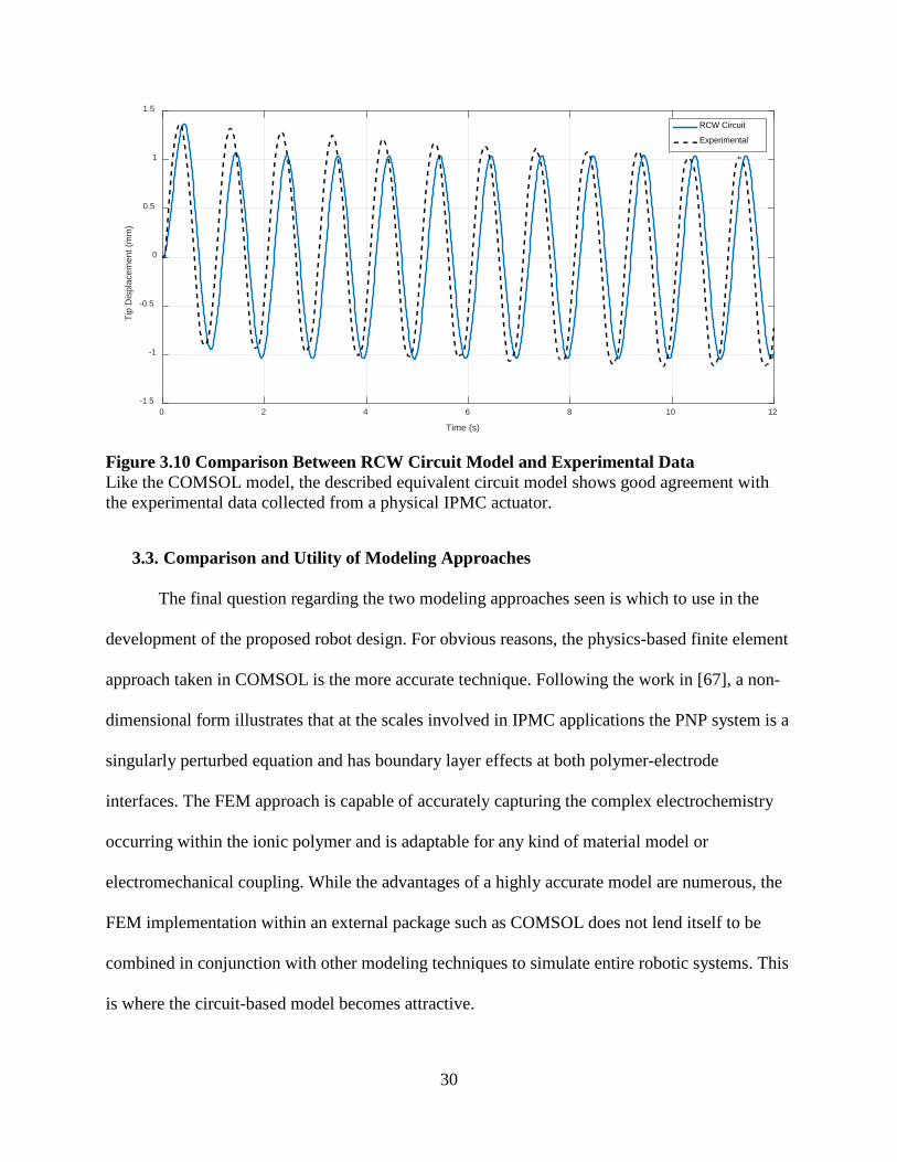
30

Figure 3.10 Comparison Between RCW Circuit Model and Experimental Data Like the COMSOL model, the described equivalent circuit model shows good agreement with the experimental data collected from a physical IPMC actuator.

3.3. Comparison and Utility of Modeling Approaches

The final question regarding the two modeling approaches seen is which to use in the

development of the proposed robot design. For obvious reasons, the physics-based finite element

approach taken in COMSOL is the more accurate technique. Following the work in [67], a non-

dimensional form illustrates that at the scales involved in IPMC applications the PNP system is a

singularly perturbed equation and has boundary layer effects at both polymer-electrode

interfaces. The FEM approach is capable of accurately capturing the complex electrochemistry

occurring within the ionic polymer and is adaptable for any kind of material model or

electromechanical coupling. While the advantages of a highly accurate model are numerous, the

FEM implementation within an external package such as COMSOL does not lend itself to be

combined in conjunction with other modeling techniques to simulate entire robotic systems. This

is where the circuit-based model becomes attractive.

Time (s)

0 2 4 6 8 10 12

Tip

Dis

plac

emen

t (m

m)

-1.5

-1

-0.5

0

0.5

1

1.5

RCW Circuit

Experimental

31

The physical basis for the circuit model is not as sound as the direct solution obtained via

FEM, but there are many methods for determining suitable parameters [3,35,70,73,88,91,92] for

a simple circuit model that yields accurate electromechanical transduction results for a given

IPMC. Furthermore, the circuit model is easily integrated into larger modeling approaches,

which will be the focus of Chapter 4.3.3, and gives researchers more flexibility with how the

mechanical deformation of the IPMC is solved. For these reasons, the circuit model will be used

for including the electromechanical effects of the IPMCs used in the proposed soft robot design.

One final comparison between both methods and the experimental data is given in Figure 3.11

for a comprehensive comparison and conclusion of the discussion in this chapter.

Figure 3.11 Comparison of FEM, Equivalent Circuit, and Experimental IPMC Deflection Here, all pair-wise comparisons between the two described models as the experimental data are provided for compactness.

Time (s)

0 2 4 6 8 10 12

Tip

Dis

plac

emen

t (m

m)

-1.5

-1

-0.5

0

0.5

1

1.5

2

RCW Circuit

Experimental

Time (s)

0 2 4 6 8 10 12

Tip

Dis

plac

emen

t (m

m)

-1.5

-1

-0.5

0

0.5

1

1.5

COMSOL

Experimental

Time (s)

0 2 4 6 8 10 12

Tip

Dis

plac

emen

t (m

m)

-1.5

-1

-0.5

0

0.5

1

1.5

2

RCW Circuit

COMSOL

Time (s)

0 2 4 6 8 10 12

Tip

Dis

plac

emen

t (m

m)

-1.5

-1

-0.5

0

0.5

1

1.5

2

RCW Circuit

COMSOL

Experimental

32

Chapter 4. Modeling of a Biomimetic Soft Robot

Prior to constructing any models of the biomimetic soft robot shown in Chapter 2, the

governing EoM must be modified to account for the differences between biological jellyfish and

the proposed design. To model the soft robot design proposed in Chapter 2, two different

approaches are taken. A preliminary model is constructed that considers the body of the robot as

a geometric surface, and that the body retains this geometric description throughout the

deformation process. The necessary derivations for the deformation, volume, and surface area

are described and the model is compared to an equivalently sized biological jellyfish. This model

is primarily used as a proof of concept of the robot design and demonstrates the feasibility of

such a robot. The second model expands the concept and spirit of the first through an

implementation of beam theory to ground the mechanical deformation of the robot body within

solid mechanics. Further derivations are given for the pertinent parameters seen in EoM, and the

equivalent circuit model for IPMCs is coupled with the beam theory implementation to model

the electro-chemo-mechanical behavior of the final robot.

4.1. Governing Equation and Model Inputs

In deriving Equation (2.11), an assumption was made that the body of a jellyfish is

approximately the same density as water. This assumption is no longer universally valid for all

constructions of the biomimetic robot as the material used to construct the body of the device

may vary in density. To remedy this, the mass of the robot is split into a persistent mass that

encompasses the materials that make up the shell of the body and the mass of water contained

within the robot. Furthermore, the added mass is an effect that occurs on the external interface

with the water, and as such its effect should be based on the external volume of the robot shell.

33

This differentiation between internal and external volume amounts to accounting for the

thickness of the material that is used to construct the robot.

Lastly, to model the effect of having directional control over the inlet and outlet of water,

the direction cosine of the outlet/inlet vector is included, as illustrated in Figure 4.1. This comes

with an assumption that these outlet/inlet locations are symmetric about the direction of travel.

For example, an inlet located perpendicular to the swimming direction would allow for the

internal volume to refill but would not contribute any acceleration to the robot, while an inlet

directed in the direction of swimming would allow for water intake and contribute a positive

acceleration to the robot. This simple addition allows for the robot to have better control over its

velocity profile during swimming and will be shown to be more effective than the swimming

mechanism of biological jellyfish.

The modified EoM can now be written as

(𝑚𝑚𝑏𝑏 + 𝜌𝜌𝑤𝑤𝑑𝑑𝑖𝑖 + 𝛼𝛼𝐴𝐴𝐴𝐴𝜌𝜌𝑤𝑤𝑑𝑑𝑓𝑓)𝑑𝑑𝑢𝑢𝑑𝑑𝑡𝑡

= cos(𝜃𝜃)𝜌𝜌𝑤𝑤𝐴𝐴𝑉𝑉

�𝑑𝑑𝑑𝑑𝑖𝑖𝑑𝑑𝑡𝑡�2

−12

Cd𝜌𝜌𝑤𝑤𝑆𝑆𝐴𝐴𝑢𝑢2 (4.1)

where 𝑚𝑚𝑏𝑏 is the mass of the robot body assumed to be fixed with a density not equal to water, 𝑑𝑑𝑖𝑖

is the internal fluid volume, 𝑑𝑑𝑓𝑓 is the external volume of the body, and cos(𝜃𝜃) is the direction

cosine illustrated in Figure 4.1. These modifications are necessary to capture a more accurate

swimming behavior of the proposed robot.

34

Figure 4.1 Illustration of Direction Cosine for Inlet and Outlet Valves The direction cosine of an inlet or outlet for the proposed design is based off the polar angle starting on the positive x-axis and trending positive counterclockwise.

In the modeling of biological jellyfish, the change in volume was assumed to be constant

during the contraction and relaxation phase with a distinct rate during each phase. In anticipation

of using an EAP actuator for the final model, a similar input source is constructed that can be

used to mimic this kind of behavior. Here, a variable amplitude and duty cycle square wave is

used as an input. This both serves to define the rate of change in volume for the original jellyfish

model, as well as model an electric potential input that could be created with a function

generator. This waveform was constructed via the Fourier series given below

𝐹𝐹(𝑡𝑡) =𝐴𝐴𝑡𝑡𝑐𝑐 + 𝐵𝐵𝑡𝑡𝑓𝑓𝑡𝑡𝑐𝑐 + 𝑡𝑡𝑓𝑓

+ �𝐴𝐴−𝐵𝐵𝑛𝑛𝑛𝑛

�𝑠𝑠𝑐𝑐𝑛𝑛 �2𝑛𝑛𝑛𝑛𝑡𝑡𝑐𝑐 + 𝑡𝑡𝑓𝑓

𝑡𝑡𝑐𝑐� 𝑐𝑐𝑐𝑐𝑠𝑠 �2𝑛𝑛𝑛𝑛𝑡𝑡𝑐𝑐 + 𝑡𝑡𝑓𝑓

𝑡𝑡�∞

𝑖𝑖=1

+ �1 − 𝑐𝑐𝑐𝑐𝑠𝑠 �2𝑛𝑛𝑛𝑛𝑡𝑡𝑐𝑐 + 𝑡𝑡𝑓𝑓

𝑡𝑡𝑐𝑐�� 𝑠𝑠𝑐𝑐𝑛𝑛 �2𝑛𝑛𝑛𝑛𝑡𝑡𝑐𝑐 + 𝑡𝑡𝑓𝑓

𝑡𝑡��

(4.2)

Direction of travel

Outlet Inlet

𝜃𝜃

35

where 𝐴𝐴 and 𝐵𝐵 are the contraction and relaxation phase amplitudes, respectively. An example of

the waveforms generated by the 3rd,.10th, and 1,000th partial sums of the Fourier series is given in

Figure 4.2. As demonstrated in the figure, the series can construct a square wave of varying duty

cycle with distinct amplitudes during each phase in a given cycle. This will be a very important

feature that is leveraged in both models further on. Later it will become relevant to references the

time ratio of relaxation time to contraction time, so it will be defined below.

Figure 4.2 Representative Waveforms Generated with Fourier Series Square Wave The characteristic contraction and relaxation phases of the jellyfish can be captured by the Fourier series shown here.

4.2. Geometry Based Modeling

4.2.1. Description of Robot Body as Geometric Surface

As discussed at the beginning of the chapter, this first modeling approach describes the

body of the robot as a geometric surface. Specifically, the shell of the robot is defined as an

ellipsoid with half-axis dimensions 𝑐𝑐, 𝑏𝑏, and 𝑐𝑐 as illustrated in Figure 4.3. This simplified

geometric approach is mainly used as a proof of concept and feasibility study, while also helping

𝛿𝛿𝑡𝑡 =𝑡𝑡𝑓𝑓𝑡𝑡𝑐𝑐

(4.3)

Time (s)

0 1 2 3 4 5 6

Ampl

itude

0.8

1

1.2

1.4

1.6

1.8

2

2.23rd Partial Sum

10th Partial Sum

1000th Partial Sum

Contraction Phase Relaxation Phase

36

aid in determining what parameters might play important roles in more robust and physics-based

modeling approaches. A constraint is placed on the model that all deformed states of the body

can be described though the definition of an ellipsoid, given by the well-known equation

Figure 4.3 Geometric Description of Robot Body as an Ellipsoid The body of the robot can be approximated as an ellipsoid for initial feasibility study of the proposed design.

4.2.2. Derivation of Model Parameters

To use a geometric approach for modeling the biomimetic robot, the volume, deformation

of the volume, cross-sectional area, drag, and added mass effects must be determined. The

internal volume of the given ellipsoid is calculated with Equation (4.5), and, with an added wall

thickness of 𝑑𝑑, the external volume with Equation (4.6) below.

𝑑𝑑𝑖𝑖 = 43𝑛𝑛𝑐𝑐𝑏𝑏𝑐𝑐 (4.5)

� 𝑥𝑥𝑐𝑐

�2

+ � 𝑦𝑦𝑏𝑏

�2

+ � 𝑧𝑧𝑐𝑐

�2

= 1 (4.4)

x

z

y

a

b c

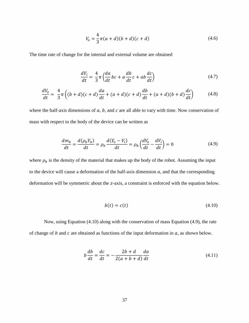
37

𝑑𝑑𝑓𝑓 =43𝑛𝑛(𝑐𝑐 + 𝑑𝑑)(𝑏𝑏 + 𝑑𝑑)(𝑐𝑐 + 𝑑𝑑) (4.6)

The time rate of change for the internal and external volume are obtained

𝑑𝑑𝑑𝑑𝑖𝑖𝑑𝑑𝑡𝑡

= 43𝑛𝑛 �

𝑑𝑑𝑐𝑐𝑑𝑑𝑡𝑡

𝑏𝑏𝑐𝑐 + 𝑐𝑐𝑑𝑑𝑏𝑏𝑑𝑑𝑡𝑡𝑐𝑐 + 𝑐𝑐𝑏𝑏

𝑑𝑑𝑐𝑐𝑑𝑑𝑡𝑡� (4.7)

𝑑𝑑𝑑𝑑𝑓𝑓𝑑𝑑𝑡𝑡

= 43𝑛𝑛 �(𝑏𝑏 + 𝑑𝑑)(𝑐𝑐 + 𝑑𝑑)

𝑑𝑑𝑐𝑐𝑑𝑑𝑡𝑡

+ (𝑐𝑐 + 𝑑𝑑)(𝑐𝑐 + 𝑑𝑑)𝑑𝑑𝑏𝑏𝑑𝑑𝑡𝑡

+ (𝑐𝑐 + 𝑑𝑑)(𝑏𝑏 + 𝑑𝑑)𝑑𝑑𝑐𝑐𝑑𝑑𝑡𝑡� (4.8)

where the half-axis dimensions of 𝑐𝑐, 𝑏𝑏, and 𝑐𝑐 are all able to vary with time. Now conservation of

mass with respect to the body of the device can be written as

𝑑𝑑𝑚𝑚𝑏𝑏

𝑑𝑑𝑡𝑡=𝑑𝑑(𝜌𝜌𝑏𝑏𝑑𝑑𝑏𝑏)𝑑𝑑𝑡𝑡

= 𝜌𝜌𝑏𝑏𝑑𝑑(𝑑𝑑𝑓𝑓 − 𝑑𝑑𝑖𝑖)

𝑑𝑑𝑡𝑡= 𝜌𝜌𝑏𝑏 �

𝑑𝑑𝑑𝑑𝑓𝑓𝑑𝑑𝑡𝑡

−𝑑𝑑𝑑𝑑𝑖𝑖𝑑𝑑𝑡𝑡� = 0 (4.9)

where 𝜌𝜌𝑏𝑏 is the density of the material that makes up the body of the robot. Assuming the input

to the device will cause a deformation of the half-axis dimension 𝑐𝑐, and that the corresponding

deformation will be symmetric about the 𝑧𝑧-axis, a constraint is enforced with the equation below.

𝑏𝑏(𝑡𝑡) = 𝑐𝑐(𝑡𝑡) (4.10)

Now, using Equation (4.10) along with the conservation of mass Equation (4.9), the rate

of change of 𝑏𝑏 and 𝑐𝑐 are obtained as functions of the input deformation in 𝑐𝑐, as shown below.

𝑏𝑏𝑑𝑑𝑏𝑏𝑑𝑑𝑡𝑡

=𝑑𝑑𝑐𝑐𝑑𝑑𝑡𝑡

= −2𝑏𝑏 + 𝑑𝑑

2(𝑐𝑐 + 𝑏𝑏 + 𝑑𝑑)𝑑𝑑𝑐𝑐𝑑𝑑𝑡𝑡

(4.11)

38

The cross-sectional area with respect to the swimming direction can be calculated based on the

external volume

𝑆𝑆𝐴𝐴 =3𝑑𝑑𝑓𝑓

4(𝑐𝑐 + 𝑑𝑑) (4.12)

Extending from the drag coefficient formulation seen in Equation (2.7), the formulation

found in [93] is used. This allows for a wide range of Reynold’s numbers, 10-1 to 106, but still

assumes a spherical body, which will introduce small errors into the model. A plot of this drag

coefficient is provided in Figure 4.4.Overall though, the results should be accurate enough for a

first approximation and feasibility study.

𝐶𝐶𝑑𝑑 = 24𝑅𝑅𝑅𝑅

+ 2.6 𝑅𝑅𝑅𝑅5.0

1 + �𝑅𝑅𝑅𝑅5.0�1.52 +

0.411 � 𝑅𝑅𝑅𝑅263000�

−7.94

1 + � 𝑅𝑅𝑅𝑅263000�

−8.00 +0.25 𝑅𝑅𝑅𝑅

106

1 + 𝑅𝑅𝑅𝑅106

(4.13)

Finally, the added mass coefficient for an ellipsoid body is found using [94]:

𝐴𝐴0 = 𝑐𝑐𝑏𝑏𝑐𝑐 ∫ 𝑑𝑑𝑊𝑊(𝑐𝑐2+𝑊𝑊)�(𝑖𝑖2+𝑊𝑊)(𝑏𝑏2+𝑊𝑊)(𝑐𝑐2+𝑊𝑊)

∞0 , 𝛼𝛼𝐴𝐴𝐴𝐴 = 𝐴𝐴0

2 −𝐴𝐴0 (4.14)

With these parameters fully defined, the EoM given in Equation (4.1) can be used to simulate the

biomimetic robot swimming.

39

Figure 4.4 Drag Coefficient as a Function of Reynold’s Number The drag coefficient correlation given in Equation (4.13) is valid over a large range of Reynold’s numbers, as shown here.

4.2.3. Comparison to Biological Jellyfish

In the proposed model, the biomimetic robot has a forward-facing inlet that, under ideal

circumstances, allows for unidirectional mass flow through the body of the robot, which will be

referenced as the P1 swimming mode. This effect manifests itself in the direction cosine term in

Equation (4.1). A side effect of allowing this kind of control is that the model can be used to

simulate a jellyfish, P2, mode, in which the inlet is directed rearward, simulating the familiar

swimming characteristics seen in Figure 2.4. The direction cosine angle for each swimming

mode is given in Table 4.1.

Table 4.1 Direction Cosine Angles for Inlet and Outlet During Different Swimming Modes

Propulsion Mode 1 (P1) Propulsion Mode 2 (P2)

Inlet 𝜃𝜃 = 0 𝜃𝜃 = 𝑛𝑛

Outlet 𝜃𝜃 = 0 𝜃𝜃 = 0

Re

10 -2 10 0 10 2 10 4 10 6

Cd

10 -2

10 -1

10 0

10 1

10 2

10 3

40

As an input to the geometric model, the rate of change of the half-axis dimension 𝑐𝑐 is

defined through the Fourier series found in Equation (4.2). A constraint is placed on the

magnitude of the contraction and relaxation amplitudes that ensures that after one complete

swimming cycle the volume returns to its initial state. This is written as

𝐵𝐵 = −𝑡𝑡𝑐𝑐𝑡𝑡𝑓𝑓𝐴𝐴 (4.15)

For an input rate of change to 𝑐𝑐 of -0.3 𝑐𝑐𝑚𝑚 𝑠𝑠⁄ , the half-axis dimension varies in time as shown in

Figure 4.5, where it is clear that the rate of change in the half-axis dimension is constant

throughout both the contraction and relaxation phases, and the constraint given by

Equation (4.15) forces the dimensions of the shell to return to their initial state after each cycle.

Figure 4.5 Input Half-Axis Dimension for Geometric Model, 1000th Partial Sum Input Using the ellipsoid model, the input half-axis dimension 𝑐𝑐 takes on the above rate of change and numeric values during deformation.

half-

axis

a (c

m)

2.35

2.4

2.45

2.5

2.55

Time (s)

0 0.5 1 1.5 2 2.5 3

half-

axis

rate

da/

dt (c

m/s

)

-0.4

-0.2

0

0.2

41

Using this input waveform, a short simulation comparing the two swimming modes is

presented in Figure 4.6. The 3rd and 1,000th partial sums are compared to illustrate the effect of

a non-ideal input. As evident from the plots, the proposed P1 mode performs better when using

the more efficient inlet/outlet directions as compared to the P2 mode. This was expected as the

mass-flux into the internal volume is in the same direction as the mass-flux out during the

contraction phase.

The effects of the non-ideal input are also expected. A lower partial sum of the Fourier

series leads to a larger transition region between contraction and relaxation phases, so the robot

slows down and begins to refill the internal volume sooner than in the idealized case. This effect

is also seen in the plot, where at approximately 𝑡𝑡 = 0.4 the robot begins to decelerate when the

non-ideal partial sum is used. This contrasts with the sharp acceleration change seen in the plot

for the idealized input. Ultimately, both input waveforms yield higher swimming performance

than the biological swimming mode, and the proposed robot design looks to be a promising

concept.

42

Figure 4.6 Simulation of Geometric Model with Various Inputs and Swimming Modes From the plots shown, the P1 swimming mode far out performs the P2 mode, and the higher partial sum that correlates to a more ideal input results in an increased performance.

A plot of the thrust profile is given in Figure 4.7 where the effect of the forward-facing

inlet is more easily seen. During the contraction phases, both thrust profiles are identical, but

when the robot body begins to relax and take water into the internal volume, the P1 mode

generates a positive thrust while the P2 mode is negative. An important consequence of this is

that the relation between contraction and relaxation time is no longer as important in generating a

net positive thrust.

Dis

tanc

e (c

m)

0

0.02

0.04P1, 3rd Partial Input

P1, 1000th Partial Input

P2, 1000th Partial InputVe

loci

ty (c

m/s

)

0

0.02

0.04

Time (s)

0 0.5 1 1.5 2 2.5 3Acce

lera

tion

(cm

/s2

)

-0.1

0

0.1

43

Figure 4.7 Thrust Profile for Geometric Model in Both Swimming Modes The P1 swimming mode shows a positive thrust profile throughout both the contraction and relaxation phases of the swimming cycle, as opposed to the positive and negative profile of the P2 swimming mode.

4.3. Physics-Based Modeling

To advance from the simplified geometric based approach taken in the previous model, a

more physics-based route is explored. Here, the deformation of the robot body will be governed

through an implementation of beam theory to describe the shell wall displacement in response to

mechanical loading from an EAP actuator. The beam theory is used to simplify the computation

of mechanical deformation by reducing the problem from the continuum model of solid

mechanics. As will be demonstrated, the use of beam theory here is modular, in the sense that

more robust and higher order models can be easily implemented in its place. Again, the

necessary model parameters for the dynamic EoM are derived and related back to the beam

theory deformation used as the method of input. Then, focusing on IPMC actuators, the

equivalent circuit model discussed before is implemented to inform the beam model on the

electromechanical response of an IPMC.

Time (s)

0 0.5 1 1.5 2 2.5 3

Thru

st (m

N)

-0.02

-0.01

0

0.01

0.02

0.03

0.04

0.05

0.06

P1 Mode

P2 Mode

44

4.3.1. Beam Theory Approach

Relating back to Figure 4.3, the new modeling approach breaks away from the constraint

of the robot body being fully defined by the equation of an ellipsoid. Instead, as illustrated in

Figure 4.8, the body is broken into active and passive regions, where the active region is

physically deformed under the IPMC loading, and the passive region is completely dictated by

the boundary conditions imposed on the geometry. Again, the deformation is assumed to be

symmetric about the z-axis. A cross-section is illustrated in, where the length measurement of the

actuator is more apparent, and the planes of symmetry are highlighted. Throughout the modeling

process, only the first quadrant of the cross-section is analyzed and the axis symmetry about the

z-axis and mirror symmetry about the xy-plane is enforced.

Figure 4.8 Diagram of Physics-Based Description of Robot Body Active portions of the robot body can be deformed using a wide variety of EAP actuators.

x

z

y

Active

Passive

45

Figure 4.9 Illustrative Cross-Section of Proposed Physics-Based Model The symmetry z-axis and xy-plane are shown in the illustration, as well as the actuator length within the active portion of the shell wall, and the radius describing the neutral axis of the beam used within the beam theory.

To describe the deformation of the shell wall, a cross-section slice along the y-z plane is

taken and the upper portion of the shell is modeled as a curved beam. Using virtual displacement,

a functional of the form below is obtained

� 𝑀𝑀𝛿𝛿𝜅𝜅 + 𝑁𝑁𝛿𝛿𝜖𝜖 − 𝑃𝑃𝑤𝑤𝛿𝛿𝑤𝑤 − 𝑃𝑃𝑣𝑣𝛿𝛿𝑣𝑣𝐿𝐿

0𝑑𝑑𝑠𝑠 = 0 (4.16)

where 𝑀𝑀, 𝑁𝑁, 𝑃𝑃, 𝑤𝑤 𝑣𝑣, and 𝑠𝑠 are the internal bending moment, internal axial load, external loading

broken into transverse (𝑃𝑃𝑤𝑤) and axial (𝑃𝑃𝑣𝑣) directions, transverse and axial displacements, and the

Sym., xy-plane

Sym., z-axis

Actuator Length

Neutral Axis

46

local axial coordinate along the length of the beam, respectively. The infinitesimal strain of the

beam is defined in terms of the curvature and axial strain, 𝜅𝜅 and 𝜖𝜖 , given by

𝜖𝜖 = 𝑣𝑣′ −𝑤𝑤𝜌𝜌

(4.17)

𝜅𝜅 = 𝑤𝑤′′ + �𝑣𝑣𝜌𝜌�′ (4.18)

where 𝜌𝜌 is the undeformed radius of curvature of the beam, assumed to be constant for

simplicity. The first terms in both strain expressions are the familiar axial and curvature strain

found in the Euler-Bernoulli beam theory for straight beams [95]. Not as familiar are the second

terms, which are couplings of the transverse and axial deformation to the axial and curvature

strains which is found only in curved beams. It can be easily verified that as the radius of

curvature tends towards infinity, these terms tend to zero and thus the straight beam theory is

recovered.

Now, the assumptions of an inextensible beam, transverse external load, and linear

elasticity are applied which yields the new functional for the beam

� 𝐸𝐸𝐼𝐼 �𝑤𝑤′′ +𝑤𝑤𝜌𝜌2�𝛿𝛿 �𝑤𝑤′′ +

𝑤𝑤𝜌𝜌2� − 𝑃𝑃𝑤𝑤𝛿𝛿𝑤𝑤

𝐿𝐿

0𝑑𝑑𝑠𝑠 = 0 (4.19)

with Young’s modulus 𝐸𝐸 and cross-sectional moment of inertia 𝐼𝐼. Using the standard virtual

displacement procedure, the functional shown can be used to construct the governing ODE for

the beam’s deformation seen below. Similarly, it can be easily shown that as the radius of

curvature tends towards infinity, the Euler-Bernoulli equation for straight beams is recovered.

𝑤𝑤𝑖𝑖𝑣𝑣 +𝑤𝑤′′

𝜌𝜌2+𝑤𝑤𝜌𝜌4

=𝑃𝑃𝑤𝑤𝐸𝐸𝐼𝐼

(4.20)

47

with a general solution obtained by solving the homogenous and particular solutions of

Equation (4.20)

𝑤𝑤(𝑠𝑠) = 𝐴𝐴𝑐𝑐𝑐𝑐𝑠𝑠 �𝑠𝑠𝜌𝜌� + 𝐵𝐵𝑠𝑠𝑐𝑐𝑛𝑛 �

𝑠𝑠𝜌𝜌� + 𝐶𝐶𝑐𝑐𝑐𝑐𝑠𝑠 �

𝑠𝑠𝜌𝜌� 𝑠𝑠 + 𝐷𝐷𝑠𝑠𝑐𝑐𝑛𝑛 �

𝑠𝑠𝜌𝜌� 𝑠𝑠 +

𝑃𝑃𝑤𝑤𝜌𝜌4

𝐸𝐸𝐼𝐼 (4.21)

In anticipation of finding an easily modified model with as close to a closed form

solution as possible, a volume integral of the form below must be calculated for use in the

dynamic EoM.

𝑑𝑑𝑖𝑖 = �𝑟𝑟2 𝑠𝑠𝑐𝑐𝑛𝑛 𝜃𝜃 𝑑𝑑𝑟𝑟𝑑𝑑𝜃𝜃𝑑𝑑𝜙𝜙 (4.22)

where 𝑟𝑟 = (𝜌𝜌 + 𝑤𝑤) describes the outer shell walls deformation, and hence internal volume. This

form depends nonlinearly on the transverse deflection, 𝑤𝑤, of the beam model. Due to the form

seen in Equation (4.21), which is entirely dependent on boundary conditions, an alternative

approach is taken to ease the work necessary to compute the volume integral.

Due to its ease in changing boundary conditions without a great deal of additional work,

the Galerkin method is used to form a trial function for the functional in Equation (4.19) to

approximate the transverse deflection. More precisely, the Galerkin method is used to construct

approximations to the deflection in terms of monomials of the local axial coordinate, seen below.

This facilitates easier calculation of the parameters used in the EoM, as will be demonstrated in

the next section. The approximation is constructed as

𝑤𝑤� = �𝑠𝑠𝑖𝑖𝑤𝑤�𝑖𝑖

𝑁𝑁𝑤𝑤

𝑖𝑖=0

= 𝑵𝑵𝑠𝑠𝒘𝒘� (4.23)

where 𝑤𝑤� is the trial function, 𝑁𝑁𝑤𝑤 is the number of monomial shape functions used, 𝑵𝑵𝒔𝒔 is a vector

of the shape functions, and 𝒘𝒘� is a vector of the Galerkin coefficients 𝑤𝑤�𝑖𝑖. Boundary conditions

48

are enforced by influencing the resulting stiffness matrix directly using the Galerkin form of the

displacement, slope, bending moment, and shear force of the beam, given below.

𝑤𝑤� = 𝑵𝑵𝑠𝑠𝒘𝒘� (4.24)

𝑤𝑤�′ = 𝑵𝑵𝑠𝑠′𝒘𝒘� (4.25)

𝑀𝑀�𝑚𝑚𝑓𝑓𝑚𝑚𝑒𝑒𝑖𝑖𝑡𝑡 = (𝑵𝑵𝑠𝑠′′ +

𝑵𝑵𝑠𝑠

𝜌𝜌2)𝒘𝒘� (4.26)

𝑑𝑑�𝑠𝑠ℎ𝑒𝑒𝑖𝑖𝑓𝑓 = (𝑵𝑵𝑠𝑠′′′ +

𝑵𝑵𝑠𝑠′

𝜌𝜌2)𝒘𝒘� (4.27)

where the moment and shear relations have been derived from the Euler-Bernoulli expressions

and introductory beam theory. Substitution of the Galerkin trial function into the functional in

Equation (4.19) results in:

𝛿𝛿𝒘𝒘�𝑻𝑻 � 𝑵𝑵𝑠𝑠𝑇𝑇 �𝐸𝐸𝐼𝐼 �𝑵𝑵𝑠𝑠

(𝑖𝑖𝑣𝑣) +𝑵𝑵𝑠𝑠′′

𝜌𝜌2+𝑵𝑵𝑠𝑠

𝜌𝜌4�𝒘𝒘� − 𝑃𝑃𝑤𝑤� 𝑑𝑑𝑠𝑠

𝐿𝐿

0 (4.28)

which can be written as:

𝑲𝑲𝒘𝒘� = 𝑷𝑷� (4.29)

with stiffness matrix and load vector defined as:

𝑲𝑲 = � 𝑵𝑵𝑠𝑠𝑇𝑇 �𝐸𝐸𝐼𝐼 �𝑵𝑵𝑠𝑠

(𝑖𝑖𝑣𝑣) +𝑵𝑵𝑠𝑠′′

𝜌𝜌2+𝑵𝑵𝑠𝑠

𝜌𝜌4�� 𝑑𝑑𝑠𝑠

𝐿𝐿

0 (4.30)

𝑷𝑷� = 𝑵𝑵𝑠𝑠𝑇𝑇𝑃𝑃𝑤𝑤 (4.31)

49

which is a system of linear equations to solve for the unknown Galerkin coefficients 𝑤𝑤�𝑖𝑖. The

integration of the stiffness matrix is achieved using Gauss-Legendre quadrature. Because the

shape functions are simple monomials, the quadrature scheme is easily implemented after a few

modifications.

The local axial coordinate is first normalized with respect to the length using the

following coordinate transformation.

𝜁𝜁 =𝑠𝑠𝐿𝐿

(4.32)

Traditional Gauss-Legendre quadrature is conducted on the domain [-1,1], so the quadrature

weights and Gauss points are transformed as well with:

𝐺𝐺𝑝𝑝′ = 1 − �1 − 𝐺𝐺𝑝𝑝

2� (4.33)

𝐺𝐺𝑤𝑤′ =𝐺𝐺𝑤𝑤2

(4.34)

Where Equation (4.33) transforms the domain [-1,1] of the traditional Gauss points to the domain

of [0,1] of the normalized local axial coordinate, and Equation (4.34) transforms the Gauss

weights accordingly to obtain the correct integration. The integrand of the stiffness matrix can

then be written as

𝑵𝑵𝜁𝜁𝑇𝑇 �𝐸𝐸𝐼𝐼 �𝑵𝑵𝜁𝜁

(𝑖𝑖𝑣𝑣) +𝑵𝑵𝜁𝜁′′

𝜌𝜌2+𝑵𝑵𝜁𝜁

𝜌𝜌4�� = 𝑁𝑁�𝜁𝜁(𝜁𝜁) (4.35)

with 𝑵𝑵𝜁𝜁 being the new shape functions in terms of the normalized length coordinate. Now the

stiffness matrix, calculated using Gauss-Legendre quadrature, becomes

50

𝑲𝑲 = 𝐿𝐿� 𝑵𝑵𝜁𝜁𝑇𝑇 �𝐸𝐸𝐼𝐼 �𝑵𝑵𝜁𝜁

(𝑖𝑖𝑣𝑣) +𝑵𝑵𝜁𝜁′′

𝜌𝜌2+𝑵𝑵𝜁𝜁

𝜌𝜌4�� 𝑑𝑑𝜁𝜁

1

0= 𝐿𝐿� 𝑁𝑁�𝜁𝜁(𝜁𝜁)𝑑𝑑𝜁𝜁

1

0= 𝐿𝐿�𝐺𝐺𝑤𝑤,𝑖𝑖

′ 𝑁𝑁�𝜁𝜁�𝐺𝐺𝑝𝑝,𝑖𝑖′ �

𝑂𝑂𝐺𝐺

𝑖𝑖=1

(4.36)

where 𝑂𝑂𝐺𝐺 is the order of the quadrature scheme. Now, with the transverse deformation able to be

computed, the condition of inextensibility can be used to determine the local axial deformation

induced in the beam.

𝜖𝜖 = 𝑣𝑣′ −𝑤𝑤𝜌𝜌

= 0 (4.37)

𝑣𝑣� =1𝜌𝜌� 𝑤𝑤�𝑑𝑑𝑥𝑥𝐿𝐿

0=

1𝜌𝜌� �𝑠𝑠𝑖𝑖𝑤𝑤�𝑖𝑖

𝑁𝑁𝑤𝑤

𝑖𝑖=0

𝐿𝐿

0𝑑𝑑𝑠𝑠 =

1𝜌𝜌�

𝐿𝐿𝑖𝑖+1

𝑛𝑛 + 1𝑤𝑤�𝑖𝑖

𝑁𝑁𝑤𝑤

𝑖𝑖=0

(4.38)

The last step in this process illustrates how the use of monomial shape functions facilitates easier

integration in the process of deriving these necessary equations. With the transverse and axial

deformations computed in a frame local to the curved beam, they can be transformed into

standard Cartesian coordinates via:

�𝑢𝑢𝑒𝑒𝑢𝑢𝑦𝑦� = � 𝑐𝑐𝑐𝑐𝑠𝑠

(𝜃𝜃𝑠𝑠) 𝑠𝑠𝑐𝑐𝑛𝑛(𝜃𝜃𝑠𝑠)−𝑠𝑠𝑐𝑐𝑛𝑛(𝜃𝜃𝑠𝑠) 𝑐𝑐𝑐𝑐𝑠𝑠(𝜃𝜃𝑠𝑠)� �

𝑣𝑣�𝑤𝑤�� (4.39)

where 𝜃𝜃𝑠𝑠 = 𝑠𝑠 𝜌𝜌� is the angle defining the position along the beam in polar coordinates with

𝜃𝜃𝑠𝑠 = 0 starting at the beginning of the beam moving in a clockwise positive direction.

An important question must be raised regarding the accuracy of the approach described.

A simple beam model on the scale expected for the proposed design was created in COMSOL in

which the continuum mechanics equations for mechanical deformation are solved under a linear

elastic assumption and serves as a benchmark for the beam model. A plot comparing the

deformation is given in Figure 4.10, while information regarding the beam geometry, material,

and loading is given in Table 4.2. From the figure it’s clear that the proposed implementation of

51

the curved beam theory is acceptable and is in very good agreement with the robust finite

element solution of the continuum equations.

Figure 4.10 Comparison of Beam Theory to FEM Implementation The proposed modeling approach where a Galerkin approximation is used to model a curved beam is shown here to be valid when compared to the COMSOL FEM solution.

Table 4.2 Beam Geometry and Loading for COMSOL Comparison

Parameter Value

Length (cm) 0.5

Width (cm) 0.25

Thickness (cm) 0.25

Modulus (cm) 50

Radius of Curvature (cm) 0.5

Load (N/m) 0.1

x-axis (cm)

0 0.1 0.2 0.3 0.4 0.5 0.6

y-ax

is (c

m)

-0.3

-0.25

-0.2

-0.15

-0.1

-0.05

0

0.05Undeformed Beam

Curved Beam Model

COMSOL

52

One more point of concern is whether the use of a curved beam model is necessary in the

given circumstance. In the limit as the radius of curvature of a beam approaches infinity, the

solution should approach that of the straight beam. Therefore, it is proposed that an accurate

measure of the effect of curvature would be to examine the error incurred in a beam’s deflection

as a function of the radius of curvature to length ratio.

Figure 4.11 demonstrates such an analysis, where the curvature aspect ratio of the beam

used in this model is highlighted and shows that a maximum percent error of approximately

3.5% is incurred when using a straight beam assumption. While this error is not necessarily

outside the range of a reasonable approximation, the ease of the Galerkin approximation makes

the decision to stay with a curved beam model obvious.

Figure 4.11 Error of Straight Beam Assumption The abscissa measures the curvature aspect ratio of a curved beam, while the ordinate is a measure of the maximum error obtained in assuming an infinite radius of curvature, i.e. a straight beam.

p/L (1)

1 2 3 4 5 6 7 8 9 10

Max

imum

Per

cent

Erro

r (%

)

0

2

4

6

8

10

Error Curve

Ratio of Beam

53

4.3.2. Derivation of Model Parameters

To derive an expression for the internal volume in this new model, Equation (4.22) is

integrated first with respect to the azimuthal angle, 𝜙𝜙, and the radial distance to obtain:

𝑑𝑑𝑖𝑖 =4𝑛𝑛3� 𝑟𝑟3 𝑠𝑠𝑐𝑐𝑛𝑛(𝜃𝜃𝑠𝑠)𝑑𝑑𝜃𝜃𝑠𝑠

𝜋𝜋2

0 (4.40)

where the symmetry of the deformation has been leveraged. The integration bounds are left as

variable because the integrand, which is dependent on the Galerkin trial function, changes as the

polar angle transitions from the active portion to the passive portion of the body. Substituting the

trial function into the expression for radial position and factoring out the dependence on the

loading and bending stiffness from the Galerkin coefficients yields

𝑟𝑟 = (𝜌𝜌 + 𝑤𝑤�) = �𝜌𝜌 +𝑃𝑃𝑤𝑤𝐸𝐸𝐼𝐼

�𝜃𝜃𝑠𝑠𝑖𝑖𝑤𝑤��𝑖𝑖

𝑁𝑁𝑤𝑤

𝑖𝑖=0

� (4.41)

where a change of variable has been made from the local axial coordinate into the polar angle,

and the Galerkin coefficients 𝑤𝑤�𝑖𝑖 have absorbed the dependence on 𝜌𝜌 from this change of

variable and become 𝑤𝑤��𝑖𝑖. The radial position is seen to have two components, the nominal radius

of curvature with an addition of the transverse deflection along the beams length. Substitution of

this into the volume integral results in the expression below.

𝑑𝑑𝑖𝑖 =4𝑛𝑛3� �𝜌𝜌3 + 3𝜌𝜌2

𝑃𝑃𝑤𝑤𝐸𝐸𝐼𝐼

�𝜃𝜃𝑠𝑠𝑖𝑖𝑤𝑤��𝑖𝑖

𝑁𝑁𝑤𝑤

𝑖𝑖=0

+ 3𝜌𝜌�𝑃𝑃𝑤𝑤𝐸𝐸𝐼𝐼

�𝜃𝜃𝑠𝑠𝑖𝑖𝑤𝑤��𝑖𝑖

𝑁𝑁𝑤𝑤

𝑖𝑖=0

�

2𝜋𝜋2

0

+ �𝑃𝑃𝑤𝑤𝐸𝐸𝐼𝐼

�𝜃𝜃𝑠𝑠𝑖𝑖𝑤𝑤��𝑖𝑖

𝑁𝑁𝑤𝑤

𝑖𝑖=0

�

3

� 𝑠𝑠𝑐𝑐𝑛𝑛(𝜃𝜃𝑠𝑠)𝑑𝑑𝜃𝜃𝑠𝑠

(4.42)

54

In what is to follow, some notation is introduced to simplify the expressions and write the

parameters for the EoM in terms of the mechanical loading. First, the summation terms risen to a

power are condensed into a single expression.

��𝜃𝜃𝑠𝑠𝑖𝑖𝑤𝑤��𝑖𝑖

𝑁𝑁𝑤𝑤

𝑖𝑖=0

�

𝑝𝑝

= 𝑊𝑊𝑝𝑝(𝜃𝜃𝑠𝑠) (4.43)

which allows Equation (4.42) to be rewritten as:

𝑑𝑑𝑖𝑖 =4𝑛𝑛3� �𝜌𝜌3 + 3𝜌𝜌2

𝑃𝑃𝑤𝑤𝐸𝐸𝐼𝐼𝑊𝑊1(𝜃𝜃𝑠𝑠) + 3𝜌𝜌 �

𝑃𝑃𝑤𝑤𝐸𝐸𝐼𝐼�2

𝑊𝑊2(𝜃𝜃𝑠𝑠) + �𝑃𝑃𝑤𝑤𝐸𝐸𝐼𝐼�3

𝑊𝑊3(𝜃𝜃𝑠𝑠)�𝑠𝑠𝑐𝑐𝑛𝑛(𝜃𝜃𝑠𝑠) 𝑑𝑑𝜃𝜃𝑠𝑠

𝜋𝜋2

0 (4.44)

Integrating this expression term by term is a cumbersome task, but can be made

significantly easier by noticing that if expanded, the integral is a series of integrals of the form

� 𝑐𝑐𝑖𝑖𝜃𝜃𝑖𝑖 𝑠𝑠𝑐𝑐𝑛𝑛 𝜃𝜃 𝑑𝑑𝜃𝜃𝛽𝛽

𝛼𝛼 (4.45)

and using integration by parts on this integral gives a series representation of the indefinite

integral, denoted by 𝐼𝐼𝑖𝑖(𝜃𝜃)

𝐼𝐼𝑖𝑖(𝜃𝜃) = 𝑐𝑐𝑐𝑐𝑠𝑠(𝜃𝜃) �(−1)𝑚𝑚+1𝑛𝑛!(𝑛𝑛 − 2𝑚𝑚)!

𝜃𝜃𝑖𝑖−2𝑚𝑚�𝑖𝑖2�

𝑚𝑚=0

+ 𝑠𝑠𝑐𝑐𝑛𝑛 (𝜃𝜃) �(−1)𝑘𝑘𝑛𝑛!

(𝑛𝑛 − 2𝑘𝑘 − 1)! 𝜃𝜃𝑖𝑖−2𝑘𝑘−1

�𝑖𝑖−12 �

𝑘𝑘=0

(4.46)

where ⌊ ⌋ is the floor operation, which gives the lowest integer value of its argument through

truncation of the decimal. This allows the definite integrals of the form Equation (4.45) to be

written as

𝐼𝐼�̅�𝑖𝛼𝛼𝛽𝛽 = 𝐼𝐼𝑖𝑖(𝛽𝛽) − 𝐼𝐼𝑖𝑖(𝛼𝛼) (4.47)

55

The integration of the internal volume can now be written in a compact form. From the

form of Equation (4.44), it is clear that the integral can be resolved into a polynomial in the

mechanical loading, with coefficients that are combinations of 𝐼𝐼�̅�𝑖𝛼𝛼𝛽𝛽 and 𝑤𝑤��𝑖𝑖. The expansion and

collection of these terms can be easily written in compact form using summations, the results of

which are given in Appendix B, where the integration bounds and are properly taken care of for

the active and passive portions of the shell. Finally, the internal volume is resolved into the cubic

polynomial shown in Equation (4.48). The simple polynomial form is a result of the Galerkin

approximation used. The time dependence of the volume has now been highlighted and stems

solely from the time variations in the loading. The beam theory used has assumed static

deflection, and thus the entire model is quasi-static, neglecting inertial effects in the mechanical

deformation.

𝑑𝑑𝑖𝑖(𝑡𝑡) =4𝑛𝑛3�𝐴𝐴0 + 𝐴𝐴1 �

𝑃𝑃𝑤𝑤(𝑡𝑡)𝐸𝐸𝐼𝐼

� + 𝐴𝐴2 �𝑃𝑃𝑤𝑤(𝑡𝑡)𝐸𝐸𝐼𝐼

�2

+ 𝐴𝐴3 �𝑃𝑃𝑤𝑤(𝑡𝑡)𝐸𝐸𝐼𝐼

�3

� (4.48)

The cross-sectional area with respect to the flow direction can be derived with a similar

approach as that taken for the volume. Specifically, the area integral necessary is:

𝑆𝑆 = �𝑟𝑟 𝑑𝑑𝑟𝑟𝑑𝑑𝜃𝜃𝑠𝑠 (4.49)

With the radial distance defined in Equation (4.41), the integral becomes:

𝑆𝑆𝐴𝐴 = 4� 𝜌𝜌2 + 2𝜌𝜌𝑃𝑃𝑤𝑤𝐸𝐸𝐼𝐼

�𝜃𝜃𝑠𝑠𝑖𝑖𝑤𝑤��𝑖𝑖

𝑁𝑁𝑤𝑤

𝑖𝑖=0

+ �𝑃𝑃𝑤𝑤𝐸𝐸𝐼𝐼

�𝜃𝜃𝑠𝑠𝑖𝑖𝑤𝑤��𝑖𝑖

𝑁𝑁𝑤𝑤

𝑖𝑖=0

�

2

𝑑𝑑𝜃𝜃𝑠𝑠𝜋𝜋2�

0 (4.50)

56

The integral is in terms of only monomials of the polar angle thus its integration is relatively

straight forward and can be evaluated to the expression below, with the coefficients 𝐵𝐵0, 𝐵𝐵1, and

𝐵𝐵2 provided in Appendix B.

𝑆𝑆𝐴𝐴(𝑡𝑡) = 𝐵𝐵0 + 𝐵𝐵1 �𝑃𝑃𝑤𝑤(𝑡𝑡)𝐸𝐸𝐼𝐼

� + 𝐵𝐵2 �𝑃𝑃𝑤𝑤(𝑡𝑡)𝐸𝐸𝐼𝐼

�2

(4.51)

For the added mass and drag coefficient, additional assumptions were made that allow the

same relations of the geometric model to be used. The added mass was initially calculated based

on an ellipsoid of largest volume that fit the material points along the x, y, and z-axis of the robot

body. After some numerical experimentation though, it was found that the added mass

coefficient maintained very small oscillations around a value of 0.5, the value for a sphere, and

due to the first approximation nature of this model the coefficient has been fixed to this value.

Since the deformation to the body is relatively small, the assumption of a spherical geometry is a

reasonable approximation. This also influences the approximation for the drag coefficient, where

the same sphere drag equation used previously has been implemented in this model.

4.3.3. Addition of IPMC Electromechanical Effects

To couple the electromechanical transduction of an IPMC to the beam theory model, the

mechanical loading of the beam, 𝑃𝑃𝑤𝑤, is related to the electrochemical behavior of the IPMC

through Equation (3.17).

𝑃𝑃𝑤𝑤 = 𝛼𝛼𝑅𝑅𝑅𝑅𝑅𝑅𝑄𝑄 (4.52)

57

Again, where the charge, 𝑄𝑄, of the IPMC is found through the Laplace transform of the RCW

circuit transfer function below.

𝑄𝑄(𝑡𝑡) = ℒ−1 �1𝑠𝑠𝐻𝐻(𝑠𝑠)ℒ{𝑑𝑑𝑒𝑒𝑒𝑒𝑡𝑡(𝑡𝑡)}� (4.53)

The Fourier series in Equation (4.2) is still used as the model input here, where it defines the

input voltage to the IPMC. Using Equation (4.53), the charge response of the IPMC to the

Fourier series input is given by

𝑄𝑄(𝑡𝑡) = 𝐴𝐴𝑡𝑡𝑐𝑐+𝐵𝐵𝑡𝑡𝑟𝑟𝑡𝑡𝑐𝑐+𝑡𝑡𝑟𝑟

2𝑐𝑐1+𝑐𝑐22

�1 − 𝑅𝑅𝑥𝑥𝑒𝑒 �− 2𝑡𝑡2𝑐𝑐3+𝑐𝑐4

��+

�𝐴𝐴−𝐵𝐵𝑛𝑛𝑛𝑛

2𝑐𝑐1 + 𝑐𝑐24 + �𝑓𝑓𝑖𝑖(2𝑐𝑐3 + 𝑐𝑐4)�

2 ��2 𝑠𝑠𝑐𝑐𝑛𝑛(𝑓𝑓𝑖𝑖𝑡𝑡𝑐𝑐) − (2𝑐𝑐3 + 𝑐𝑐4)𝑓𝑓𝑖𝑖(1 − 𝑐𝑐𝑐𝑐𝑠𝑠(𝑓𝑓𝑖𝑖𝑡𝑡𝑐𝑐))�𝑐𝑐𝑐𝑐𝑠𝑠(𝑓𝑓𝑖𝑖𝑡𝑡)∞

𝑖𝑖=0+

(2(1 − 𝑐𝑐𝑐𝑐𝑠𝑠(𝑓𝑓𝑖𝑖𝑡𝑡𝑐𝑐)) + (2𝑐𝑐3 + 𝑐𝑐4)𝑓𝑓𝑖𝑖 𝑠𝑠𝑐𝑐𝑛𝑛(𝑓𝑓𝑖𝑖𝑡𝑡𝑐𝑐))𝑠𝑠𝑐𝑐𝑛𝑛(𝑓𝑓𝑖𝑖𝑡𝑡) +

�(2𝑐𝑐3 + 𝑐𝑐4)𝑓𝑓𝑖𝑖(1 − 𝑐𝑐𝑐𝑐𝑠𝑠(𝑓𝑓𝑖𝑖𝑡𝑡𝑐𝑐)) − 2 𝑠𝑠𝑐𝑐𝑛𝑛(𝑓𝑓𝑖𝑖𝑡𝑡𝑐𝑐)�𝑅𝑅𝑥𝑥𝑒𝑒 �−2𝑡𝑡

2𝑐𝑐3 + 𝑐𝑐4��

(4.54)

with

𝑐𝑐1 = 𝐶𝐶, 𝑐𝑐2 = 𝑊𝑊, 𝑐𝑐3 = 𝑅𝑅𝐶𝐶, 𝑐𝑐4 = 𝑅𝑅𝑊𝑊, 𝑓𝑓𝑖𝑖 =2𝑛𝑛𝑛𝑛𝑡𝑡𝑐𝑐 + 𝑡𝑡𝑓𝑓

(4.55)

The charge response to a representative input for the model is given in Figure 4.12. The

capacitive charge and discharge profiles are clearly visible, and even in this short simulation the

beginning of the decay to a steady state response is seen in the peaks of the charge during the

contraction phases.

58

Figure 4.12 RCW Model Charge Response for Fourier Series Input Noting the input voltage, the charge response shows a non-net-zero charge over each swimming cycle due to the equal voltage amplitudes over different time periods. This can be remedied with an input that follows the constraint of Equation (4.15).

4.3.4. Evaluation and Comparison to Previous Model

A comparison of the swimming behavior of this physics-based model to the two previous

models is given in Figure 4.13. For the comparison, the original model in Chapter 2 was used. A

jellyfish of comparable size and volume exchange was modeled, the parameters of which are

given in Table 4.3. An important note must be made here. The simulation of the biological

jellyfish used was matched to a comparable volume exchange of the two proposed models. From

[58], the typical volume change for a jellyfish is on the order of 50%, where here a change of

only 7.5% is used. While Figure 4.13 demonstrates that the two proposed biomimetic robot

models do perform better than the biological counter-part, the biological jellyfish model is not

operating at full capacity.

This comes from the limitations on the amount of deformation allowed within the newly

proposed physics-based model. By using a linear beam theory, small strain limitations do not

0 2 4 6 8 10 12 14 16

Volta

ge (V

)

-5

0

5

Time [s]

0 2 4 6 8 10 12 14 16

Cha

rge

(C)

-2

-1

0

1

2

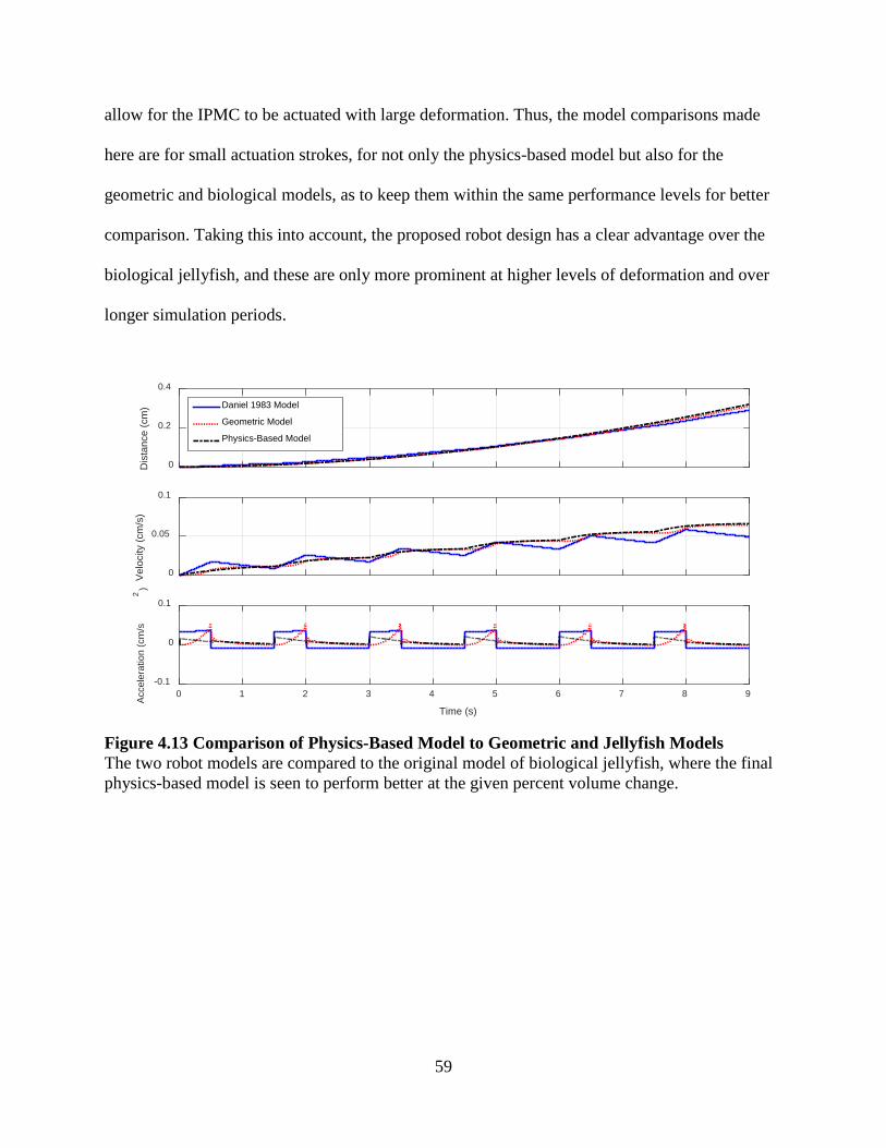
59

allow for the IPMC to be actuated with large deformation. Thus, the model comparisons made

here are for small actuation strokes, for not only the physics-based model but also for the

geometric and biological models, as to keep them within the same performance levels for better

comparison. Taking this into account, the proposed robot design has a clear advantage over the

biological jellyfish, and these are only more prominent at higher levels of deformation and over

longer simulation periods.

Figure 4.13 Comparison of Physics-Based Model to Geometric and Jellyfish Models The two robot models are compared to the original model of biological jellyfish, where the final physics-based model is seen to perform better at the given percent volume change.

Dis

tanc

e (c

m)

0

0.2

0.4

Daniel 1983 Model

Geometric Model

Physics-Based Model

Velo

city

(cm

/s)

0

0.05

0.1

Time (s)

0 1 2 3 4 5 6 7 8 9

Acce

lera

tion

(cm

/s2

)

-0.1

0

0.1

60

Table 4.3 Physics-Based Model Comparison Parameters

Parameter Value

Daniel 1983 Geometric Physics-Based

Radius of Body (mm) ~ 25.4 25.4

Height of Bell (mm) 25.4 ~ ~

Half-Axis Rate (mm/s) ~ 3 ~

Volume Change (%) 7.5 ~ ~

IPMC Length (mm) ~ ~ 20.5

IPMC Width (mm) ~ ~ 9.94

IPMC Thickness (mm) ~ ~ 0.57

Voltage (V) ~ ~ 4

Contraction Time (s) 0.5 0.5 0.5

Time Ratio (1) 2 2 2

Outlet Radius (mm) 12.7 1 1

Evaluating the physics-based model on its own, the thrust profile given in Figure 4.14 for

both P1 and P2 swimming modes is reminiscent of the geometric model. The biomimetic mode

shows a constant positive thrust where the relaxation phase component is seen to be mirror over

the zero-line. Furthermore, the longer simulation allows for the transient behavior of the initial

IPMC actuation to be more easily seen. The peak thrust during the contraction phase is at the

initial contraction, which is followed by a steep decay in thrust. Similarly, the relaxation phase

sees a high initial thrust value, followed by a slower decay until the next contraction occurs. This

is due to the initial expelling or intake of water and can be directly related to the mass flux

through the system, as shown in Figure 4.15.

61

Figure 4.14 Thrust Profile for Physics-Based Model As seen before for the geometric based model, the physics-based model shows a positive thrust profile throughout the swimming cycle in the P1 swimming mode.

Figure 4.15 Mass Flux for Physics-Based Model The mass flux throughout the body of the robot is characteristic of the momentum exchanged through the fluid pumped out of the device.

Time (s)

0 1 2 3 4 5 6 7

Thru

st (m

N)

-0.01

-0.005

0

0.005

0.01

0.015

0.02P1 Mode

P2 Mode

Time (s)

0 1 2 3 4 5 6 7

Mas

s Fl

ux (k

g/s)

10 -4

-2.5

-2

-1.5

-1

-0.5

0

0.5

1

1.5

62

Observing the mass flux profile, during the contraction phase there is a negative flux as

water leaves the internal volume. If a control volume is drawn at the outlet of the robot, and if

the robot were constrained and fixed in place, the fluid motion through the control volume may

be plotted. The ejected fluid through the control volume has a velocity given by

𝑣𝑣𝑒𝑒 =�̇�𝑚

𝜌𝜌𝑤𝑤𝐴𝐴𝑣𝑣 (4.56)

where �̇�𝑚 is the mass flux through the control volume. It can be easily visualized that during the

relaxation phase, the velocity through this control volume is zero, assuming the inlet is forward

facing. Thus, the system now behaves as a unidirectional fluid pump. Clearly, the longer the

relaxation phase is the more pulsating the flow through the control volume becomes. If the time

ratio for the robot is then lowered, the velocity through the control volume becomes more

continuous. This is illustrated in Figure 4.16, where velocity profiles for the device in normal

operation and the described low time ratio are shown for comparison.

This type of operation transforms the robot into a fluid pump, allowing for a near

constant mass flow or a pulsating flow, making it suitable for multiple applications in low

volume fluid pumping, akin to the proposed design in [96]. An interesting feature is the

unidirectional aspect of this pump, where using one-way valves inherent in the structure of the

shell, back flow is restricted. The IPMC driven actuation also makes the system a low voltage

component. An alternative input voltage waveform may also allow for a more uniform flow

velocity, but this is a question for future optimization and experimentation.

63

Figure 4.16 Velocity Profiles for Fluid Pump Operation Fluid velocity profile at outlet of device. The outlet fluid velocity during a swimming operation shows the distinct pulse during contraction phases. By extending the contraction phase over a longer period and shortening the relaxation phase, the outlet velocity becomes more continuous and the device may be used as a fluid pump. (Top) Swimming operation. (Bottom) Fluid pumping operation.

Time (s)

0 1 2 3 4 5 6 7

Flui

d Ve

loci

ty (c

m/s

)

0

5

10

Time (s)

0 1 2 3 4 5 6 7 8 9 10 11

Flui

d Ve

loci

ty (c

m/s

)

0

5

10

64

Chapter 5. Design Optimization

With a physics-based model for the swimming behavior of the proposed robot, there is a

question of whether the original design can be improved upon. Here, a simple design

optimization is conducted to search for model parameters that give largest swimming distance

over a given period. To conduct the optimization, a sequential quadratic programming (SQP)

routine is implemented in MATLAB on a few, hand selected design parameters. These

parameters are investigated from a qualitative view to gain some understanding of how they

might interact with each other during the optimization process. From there, an optimization

routine is run to search for the optimal parameters, and the newly optimized design is compared

to the originally proposed model. Some preliminary work on the scalability of the device is also

presented and a discussion on the limitations of the model as it relates to its optimization

capabilities is discussed.

5.1. Sequential Quadratic Programming Optimization

5.1.1. Selection of Design Variables

The design variables selected for optimization were chosen manually with some insight

into the model and its limitations. Of all the possible variables involved in the physics-based

model, the three chosen as design parameters were the IPMC length, contraction time, and time

ratio. Other parameters, such as IPMC thickness, IPMC width, valve aperture, input voltage, and

many more have significant effects on the performance of the robot, but due to a few model

limitations which will be discussed later, these were not viable selections.

As expected, the IPMC length plays an important role, but its exact effects on the

performance of the robot were not fully understood. To begin the optimization process, the

65

model was made into an executable MATLAB function that took an input of the IPMC length

and would output the maximum distance traveled over a 30 second period. This gives a

qualitative understanding of how the parameter affects the swimming behavior. The results of

this numerical experiment are given in Figure 5.1, where there is a noticeable peak in

performance around 𝐿𝐿 = 26 (mm). While the increase in performance with increasing length was

expected, the rapid decay in distance traveled when passing the peak value was not. This is

attributed to the degree the shell wall is deformed as the length increases. After the length passes

the observed optimal value, the contraction and relaxation phases switch roles in the sense that

during the “contraction” phase, the internal volume is increased, and the “relaxation” phase sees

a decrease in volume. This effectively changes the operation behavior of the device and when

keeping the contraction time and time ratio constant, this results in decreased performance. The

parameters for the model simulation are given in Table 5.1.

Figure 5.1 Distance vs IPMC Length A simple plot of distance traveled as a function of IPMC length shows that an optimal value for the length is located near 26 (mm).

Length (mm)

0 5 10 15 20 25 30 35

Dis

tanc

e Tr

avel

ed (c

m)

0

0.2

0.4

0.6

0.8

1

66

Table 5.1 Simulation Parameters for IPMC Length Optimization

Parameter Value

Simulation Time (s) 30

Time Step (s) 0.001

Contraction Time (s) 0.5

Time Ratio (1) 2

To gain further insight in the design variables in question, a surface plot of distance

traveled was constructed for the pairwise combinations of the three parameters. These surface

plots are a kind of brute force optimization aid where one can visually identify the trends in the

performance of the model based on the two-parameter combination. Since the approach requires

repeated simulations, the accuracy of the model has been sacrificed to a degree to speed up the

process, as reflected by the increased time step shown in Table 5.2. Because these surface plots

are more qualitative, the loss in accuracy is not an issue, and a more robust optimization will be

conducted in the next chapter.

The surface plot for the combination of IPMC length and the contraction time shows an

unsurprising trend. The familiar optimal value for the length parameter is evident, and a

monotonically decreasing distance in the contraction time is seen. These results are expected, but

it at least verifies the behavior seen in Figure 5.1. Turning to the plot of IPMC length and the

time ratio, the surface profile is a little more interesting. The profile observed in Figure 5.1 is still

prevalent, but the behavior of the surface shows a global maximum near a time ratio value of

𝛿𝛿𝑡𝑡 ≅ 2.5. This means that there may be an optimal design solution in this neighborhood that

could be found using a more robust optimization routine. For now, it will be taken only for a

qualitative understanding of where a more optimal design may reside. Finally, the results of

pairing the contraction time and time ratio give a predictable surface plot. The monotonically

67

decreasing behavior of the contraction time is evident while the peak value associated with the

time ratio discussed previously is clearly seen. These qualitative results are presented in Table

5.3, where the original unoptimized design parameters are listed alongside of the expected

optimal parameter values.

Table 5.2 Simulation Parameters for Pairwise Optimization

Parameter Value Range

Simulation Time (s) 20 ~

Time Step (s) 0.005 ~

Contraction Time* (s) 0.5 0.2-2

Time Ratio* (1) 2 1-10

Length* (mm) 20.5 5-35

* Indicates the value taken when the variable is not selected as design parameter for optimization plots.

Figure 5.2 Surface Plot of Distance vs Length and Contraction Time The two-parameter surface plot shows the interaction between the length and contraction time and their effect on distance traveled.

3530

25

Length (mm)

2015

105

0.5Contraction Time (s)

1

1.5

0.6

0.4

0.2

0

0.8

2

Dis

tanc

e Tr

avel

ed (c

m)

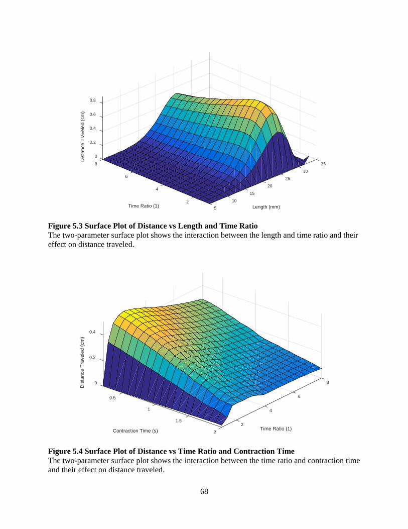
68

Figure 5.3 Surface Plot of Distance vs Length and Time Ratio The two-parameter surface plot shows the interaction between the length and time ratio and their effect on distance traveled.

Figure 5.4 Surface Plot of Distance vs Time Ratio and Contraction Time The two-parameter surface plot shows the interaction between the time ratio and contraction time and their effect on distance traveled.

3530

25

Length (mm)

2015

105

2Time Ratio (1)

4

6

0.2

0

0.8

0.6

0.4

8

Dis

tanc

e Tr

avel

ed (c

m)

8

Time Ratio (1)

6

4

2

2

1.5

Contraction Time (s)

1

0.5

0.2

0.4

0

Dis

tanc

e Tr

avel

ed (c

m)

69

Table 5.3 Parameter Values for Unoptimized and Expected Optimal Designs

Parameter Unoptimized Design Expected Optimal Value

IPMC Length (mm) 20.5 26

Contraction Time (s) 0.5 0.2

Time Ratio (1) 2 2.5

5.1.2. Optimization of Design Variables

There are numerous methods for constrained nonlinear optimization, many of which are

excellently described in [97]. To conduct a more thorough optimization of these design

parameters, an implementation of the SQP method is performed in MATLAB using the fmincon

function. This algorithm is capable of handling constrained nonlinear optimization problems.

The constraints used here consist only of bounding limits on the design variables and an

inequality constraint on the IPMC length. The boundary limits are given as

10 < 𝐿𝐿𝑖𝑖𝑝𝑝𝑚𝑚𝑐𝑐 ≤ 𝑛𝑛2𝜌𝜌 − 𝜖𝜖𝐿𝐿 (5.1)

1 < 𝛿𝛿𝑡𝑡 < 5 (5.2)

0.05 < 𝑡𝑡𝑐𝑐 < 2 (5.3)

where 𝜖𝜖𝐿𝐿 is the minimum amount of passive material that makes up the shell wall after the end of

the IPMC. The inequality constraint ensures that the length of the IPMC does not exceed the

hemisphere that is being modeled after symmetry planes have been addressed. The remaining

boundaries for the design parameters have been chosen based on experience with the model. The

lower boundary for the time ratio is chosen such that the relaxation time will be no shorter than

the contraction, which is an implied assumption in the development of this model. The upper

70

boundary on the time ratio as well as the boundaries for the contraction time have been chosen to

provide a large solution space for the optimization to search within.

To make sure that the optimal solution obtained through this method is accurate, multiple

implementations of the algorithm are conducted, each starting from an initial condition that is

randomly perturbed. This ensures that more of the solution space is explored by the algorithm,

and by collecting multiple solutions statistical metrics can be collected to verify the accuracy of

the obtained values. The initial values and perturbations applied to them are given in Table 5.4,

along with the simulation parameters used. The perturbations are applied via

𝑋𝑋𝑖𝑖,0 = 𝑥𝑥𝑖𝑖 + 𝛿𝛿𝑖𝑖 𝑟𝑟𝑖𝑖,1(−1)�𝑓𝑓𝑖𝑖,2� (5.4)

where 𝑋𝑋𝑖𝑖,0 is the ith parameter’s initial value, 𝑥𝑥𝑖𝑖 is the parameter’s nominal value, 𝛿𝛿𝑖𝑖 is the

perturbation of the parameter, 𝑟𝑟𝑖𝑖,1 and 𝑟𝑟𝑖𝑖,2 are distinct random numbers generated for the

parameter, and ⌊ ⌉ denotes the rounding operator, which outputs the integer value obtained after

rounding its argument up or down depending on the leading digit of the decimal. This approach

scales the value of each parameter by a range associated with the perturbation in both positive

and negative directions based on two randomly generated numbers, thus ensuring that each

successive implementation of the SQP algorithm begins at a different initial point.

71

The SQP function is implemented with the constraints given in Equations (5.1)-(5.3) with

an initial condition obtained from Equation (5.4). Here, the routine was run for 100 trials, with

the results of each being retained so that the mean and standard deviation for each of the

resulting design parameters could be calculated. Random variables are uniformly distributed over

the range [0,1].

Table 5.4 Parameters for SQP Optimization of Design Variables

Parameter Value Perturbation

Simulation Time (s) 30 ~

Time Step (s) 0.005 ~

IPMC Length* (mm) 20.5 5

Time Ratio* (1) 2 1

Contraction Time* (s) 0.5 0.1

Passive Material, 𝜖𝜖𝐿𝐿 (mm) 5 ~

* Indicates the nominal value used in (5.4)

After 100 successive SQP routines, the resulting optimal parameters obtained were

processed into the probability density functions for the IPMC length, time ratio, and contraction

time shown in Figure 5.5, Figure 5.6, and Figure 5.7, respectively. The mean and standard

deviation for these results are provided in Table 5.5, where it is clear that the final optimal values

are in good agreement with the expected results obtained from the surface plots.

Of interest is how precise the results are for the IPMC length, evident from both the

probability density function as well as the small standard deviation. Similarly, the contraction

time shows a more compact distribution, indicating that the mean value obtained is more likely

to be the ideal value. The time ratio shows a wider distribution, corresponding to its larger

standard deviation. This implies that the result obtained is not as significant for the optimal

72

design. This is also expected from the form of the surface plots shown previously, where the

decay in performance was not as significant for changes in the time ratio as compared to the

contraction time or length.

Figure 5.5 Probability Density Function: IPMC Length The probability density function for the IPMC length helps in visualizing the certainty in the optimal value obtained.

Figure 5.6 Probability Density Function: Time Ratio The probability density function for the time ratio helps in visualizing the certainty in the optimal value obtained.

Length (cm)

5 10 15 20 25 30 35

Prob

abilit

y D

ensi

ty

0

0.05

0.1

0.15

0.2

0.25

0.3

0.35

Time Ratio (1)

1 1.5 2 2.5 3 3.5 4 4.5 5

Prob

abilit

y D

ensi

ty

0

0.2

0.4

0.6

0.8

73

Figure 5.7 Probability Density Function: Contraction Time The probability density function for the contraction time helps in visualizing the certainty in the optimal value obtained.

Table 5.5 Results of SQP Optimization

Parameter Mean Value Standard Deviation

IPMC Length (mm) 25.8 1.32

Time Ratio (1) 2.31 0.502

Contraction Time (s) 0.462 0.171

5.2. Comparison of Unoptimized and Optimized Design

The newly optimized model has been compared to the original unoptimized model for

both the P1 and P2 swimming modes. As demonstrated in Figure 5.8, the optimized model far

outperforms the unoptimized design. In both swimming modes, the optimal design shows an

improvement of approximately a factor of 2 in terms of distance traveled. Again, the advantages

of the P1 mode out performances P2, as expected. This strongly indicates that the proposed

design may be useful in developing a high performance, highly efficient soft robot for aquatic

applications.

Contraction Time (s)

0 0.2 0.4 0.6 0.8 1 1.2 1.4 1.6 1.8 2

Prob

abilit

y D

ensi

ty

0

0.5

1

1.5

2

2.5

74

Figure 5.8 Comparison of Unoptimized and Optimized Models: Distance Traveled Top: Comparison of distance in P2 swimming mode. Bottom: Comparison of distance in P1 swimming mode.

A quantitative comparison between the unoptimized and optimized model can be

obtained by examining the propulsion efficiency of the two models at steady state. This

efficiency is calculated using

𝜂𝜂𝑝𝑝𝑓𝑓𝑓𝑓𝑝𝑝 =2

1 +𝑣𝑣𝑓𝑓𝑓𝑓𝑊𝑊𝑖𝑖𝑑𝑑𝑣𝑣𝑓𝑓𝑓𝑓𝑏𝑏𝑓𝑓𝑡𝑡

(5.5)

where 𝑣𝑣𝑓𝑓𝑓𝑓𝑊𝑊𝑖𝑖𝑑𝑑 and 𝑣𝑣𝑓𝑓𝑓𝑓𝑏𝑏𝑓𝑓𝑡𝑡 are the fluid velocity and robot velocity, respectively. As evident from

the equation, as the robot velocity matches that of the fluid the efficiency approaches unity, and

as the robot velocity drops lower than the fluid, the efficiency approaches zero. These

efficiencies are calculated individually, at steady state, over the final contraction and relaxation

0 5 10 15 20 25 30

Dis

tanc

e Tr

avel

ed (c

m)

0

0.5

1

1.5

2

Unoptimized

Optimized

Time (s)

0 5 10 15 20 25 30

Dis

tanc

e Tr

avel

ed (c

m)

0

2

4

6

Unoptimized

Optimized

75

cycle, and the result is averaged to obtain the propulsion efficiency for the robot in each

swimming mode. These results are tabulated in Table 5.6, along with the average thrust

generated over the entire swimming cycle. Figure 5.9 shows the resulting velocity plots for the

two models in both the P1 and P2 swimming modes.

Table 5.6 Propulsion Efficiency for Unoptimized and Optimized Models

Model Swimming Mode Efficiency (%) Mean Thrust (𝝁𝝁N)

Unoptimized P1 10.8 8.20

P2 5.06 2.58

Optimized P1 11.6 14.2

P2 6.27 5.38

Figure 5.9 Velocity Profiles for Efficiency Calculation Top: Profile for swimming velocity during P2 mode. Upper profile is the optimized model. Bottom: Profile for swimming velocity during P1 mode. Upper profile is the optimized model.

0 50 100 150

Velo

city

(cm

/s)

0

0.05

0.1

0.15

0.2

0.25

Unoptimized

Optimized

Time (s)

0 50 100 150

Velo

city

(cm

/s)

0

0.1

0.2

0.3

0.4

Unoptimized

Optimized

76

The results shown in Figure 5.9 again show a factor increase in velocity of approximately

2 for the optimal design as compared to the unoptimized approach. One further point of interest

is that the more efficient swimming behavior of the biomimetic mode leads to the robot reaching

its steady state behavior more rapidly. This is evident in the profile of the velocity plots, where

the P1 swimming mode is seen to reach its steady state around 50 seconds, whereas the P2 mode

takes approximately twice as long.

5.3. Scale Effects on Optimal Parameter Values

To gain insight into how the proposed robot design might scale, a second implementation

of the SQP optimization was undertaken. Here, the size of the robot body is scaled, and the

optimization routine is used to determine how the chosen design variable’s optimal value vary

with the size of the robot. There are some limitations regarding the model that limit the physical

size of the robot, but these will be elaborated on further in the discussion section of this chapter.

Firstly, the boundaries of the design variables that have the units of length are scaled to

the original body radius of 25.4 (mm), thus ensuring that the solution space scales along with the

size of the robot. The SQP routine is then used to find an optimal parameter set for five different

robot sizes over 25 trials. Data from all 25 optimization routines for each robot size are then used

to construct statistics necessary to quantify the results. The final values obtained after this

process are tabulated in Table 5.7, where a few interesting trends are seen.

When looking down the column for the IPMC length, there is a clear linear trend that is

almost one to one in terms of IPMC length and shell radius. Furthermore, the time ratio and

contraction time seem to have no dependence on the size of the robot. As seen from the standard

deviation, the results seem to become not as precise as the size of the robot scales up. This may

77

be an implication that as the robot becomes larger, the model no longer has as well defined of an

optimal solution as compared to the smaller devices.

Table 5.7 Results of Optimization with Scaled Shell Radius

Radius of Shell (mm)

Optimal Value, Mean / Std. Dev.

IPMC Length (mm) Time Ratio (1) Contraction Time (s)

10 10.7 / 0.951 2.11 / 0.557 0.418 / 0.125

20 20.2 / 0.104 2.17 / 0.550 0.427 / 0.128

30 30.7 / 2.22 2.30 / 0.544 0.438 / 0.236

40 40.1 / 0.202 2.48 / 0.380 0.551 / 0.363

50 52.6 / 7.31 2.52 / 0.895 0.840 / 1.23

The data given in Table 5.7 is also presented in Figure 5.10, Figure 5.11, and Figure 5.12,

where the trends are much easier to visualize. As evident in the data shown in the figures, as the

shell radius increases, the precision of the SQP optimization decreases.

Figure 5.10 Optimized IPMC Length Versus Radius of Shell The above figure shows the linear trend of the optimized IPMC length as a function of the shell radius. Equation (5.6) gives the regression line shown, where the slope is shown to be near unity.

Radius of Shell (mm)

0 10 20 30 40 50

Opt

imal

IPM

C L

engt

h (m

m)

0

10

20

30

40

50

60Fitted Linear Trendline

SQP Results

78

Figure 5.11 Optimized Time Ratio Versus Radius of Shell Here, a near constant trend is seen in the SQP results, with a much wider range of values. This is expected as during the initial SQP optimization the time ratio was seen to have a less well defined optimal value.

Figure 5.12 Optimized Contraction Time Versus Radius of Shell Similarly, the contraction time shows a more constant trend as a function of the shell radius. This is also explained in the previous optimization analysis.

Radius of Shell (mm)

0 10 20 30 40 50

Opt

imal

Tim

e R

atio

(1)

0

1

2

3

4

5 Fitted Linear Trendline

SQP Results

Radius of Shell (mm)

0 10 20 30 40 50

Opt

imal

Con

tract

ion

Tim

e (s

)

0

1

2

3

4Fitted Linear Trendline

SQP Results

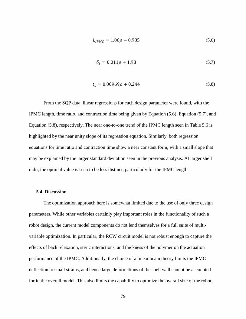
79

𝐿𝐿𝐼𝐼𝐼𝐼𝐴𝐴𝑅𝑅 = 1.06𝜌𝜌 − 0.985 (5.6)

𝛿𝛿𝑡𝑡 = 0.011𝜌𝜌 + 1.98 (5.7)

𝑡𝑡𝑐𝑐 = 0.00969𝜌𝜌 + 0.244 (5.8)

From the SQP data, linear regressions for each design parameter were found, with the

IPMC length, time ratio, and contraction time being given by Equation (5.6), Equation (5.7), and

Equation (5.8), respectively. The near one-to-one trend of the IPMC length seen in Table 5.6 is

highlighted by the near unity slope of its regression equation. Similarly, both regression

equations for time ratio and contraction time show a near constant form, with a small slope that

may be explained by the larger standard deviation seen in the previous analysis. At larger shell

radii, the optimal value is seen to be less distinct, particularly for the IPMC length.

5.4. Discussion

The optimization approach here is somewhat limited due to the use of only three design

parameters. While other variables certainly play important roles in the functionality of such a

robot design, the current model components do not lend themselves for a full suite of multi-

variable optimization. In particular, the RCW circuit model is not robust enough to capture the

effects of back relaxation, steric interactions, and thickness of the polymer on the actuation

performance of the IPMC. Additionally, the choice of a linear beam theory limits the IPMC

deflection to small strains, and hence large deformations of the shell wall cannot be accounted

for in the overall model. This also limits the capability to optimize the overall size of the robot.

80

As mentioned earlier, when attempting to optimize the size of the robot, the constrained

on the IPMC length is very important. The model is not capable of handling a zero-percentage of

passive material in the shell wall, and as such there must be some constraint in place to ensure

that as the size of the robot increases the IPMC does not fully eliminate the passive portion in the

design. Furthermore, from experience with the IPMC actuators, there is a tradeoff between

performance and length, whereas the IPMC scales its actuation capabilities degrade. This

phenomenon is not currently captured within the proposed models, and hence the scale effects on

optimization demonstrated here are not valid at the larger size of robots. With the limitations of

the circuit model in predicting the behavior of the IPMC at larger sizes, the optimization of the

overall size and geometry of the robot is currently not feasible.

81

Chapter 6. Conclusion

Biology has been shown to provide invaluable inspiration for the modeling, design, and

development of soft robotic systems. Here, insight of the jet propulsion mechanism found in

jellyfish lead to a new theory about an improved swimming mechanism for small aquatic robots.

A robust finite element model of the complex Poisson-Nernst-Planck system of equations

for IPMC actuation was described, wherein a reduction in the problem’s dimensionality was

leveraged to drastically improve on the computational overhead required to solve these complex

Multiphysics problems. The described approach was shown to give highly accurate results in

good agreement with other modeling approaches found in literature. This was achieved by

solving the PNP system in 1D and using a mapping equation to transform the results on this

lower dimensional domain onto a full 2D domain, where the electromechanical transduction was

solved and the IPMC displacement was calculated. This finite element model was then shown to

be in good agreement with experimental data taken from an actual IPMC.

Similarly, an equivalent circuit model was described which included resistive, capacitive,

and Warburg impedances. The circuit model provides a quick, easy to implement, and highly

modular model for the electrochemical behavior of IPMC actuators. This approach, when

combine with an electromechanical coupling equation, can be used to model IPMC actuator

displacement in response to an external voltage input. Using a straight beam model, the circuit

model was shown to be in good agreement with both experimental data as well as the complex

finite element implementation.

Using a simplified geometrically defined model, the proposed biomimetic robot design

was proved to be at least feasibly and to provide potential efficiency improvements over its

biological inspiration. A simple ellipsoid geometry was found to provide a useful tool for the

82

description of a robotic system but lacked a physical basis that was desired for a more well-

defined model. The model still provided some critical information and insight into how a robot

of this design may function and behave as compared to its biological jellyfish inspiration.

The simplified geometric approach was improved upon by starting from a physical basis,

namely, a beam theory found in the field of solid mechanics. Due to the spherical design, a linear

curved beam was proposed and the deformation of such beam under a uniformly distributed load

was calculated approximately through a Galerkin trial function. The trial function was

specifically chosen to include only monomial terms so that future endeavors for developing a

dynamic model for the swimming behavior would be easier to express mathematically. The

choice of trial function was shown to be extremely useful in describing the internal volume and

cross-sectional area for the physics-based model. The model was then completed by coupling the

equivalent circuit model for IPMC deformation with the curved beam theory used to provide a

fast and accurate modeling approach that is grounded in physical principles. The physics-based

approach was found to be in good agreement with both the geometric and biological jellyfish

models for the swimming regimes tested. Using the newly developed model, the ability for the

proposed robot design be used as a low volume fluid pump was described. By changing how the

device was constrained and examining a small control volume at the outlet of the system, it was

shown that it is possible to generate nearly continuous flow or pulsating flow from the same

device while relying only on low voltage inputs for the IPMC actuators.

Finally, an optimization of the design was conducted. A few design parameters were

chosen and their effect on the distance traveled by the robot was modeled. After narrowing down

on three parameters, namely the IPMC length, contraction time, and time ratio, surface plots of

the robot’s displacement were created to gain some valuable insight into the existence of a

83

possible optimal parameter set. From there, an implementation of sequential quadratic

programming was used to find the exact optimal solution. In this optimization, 100 trials were

used to construct mean and standard deviations of the design variables to verify that the

optimization routine found a good maximum. From the results obtained, the optimal solution was

verified, and the optimal model was compared to the original unoptimized implementation. The

optimal parameters were shown to increase performance significantly, evident from plots of the

distance traveled over time as well as comparing the average thrust and propulsion efficiency. A

look at the scale effects on the optimal design parameters was taken, and it was shown that as the

robot increases in size, the IPMC actuator necessary to achieve optimal performance also must

increase linearly. The limitations of the model with regard to optimization were discussed.

Specifically, the linear deflection and limited circuit model do not allow for a more complex

multi-variable optimization with scaling to be conducted. This is an important topic for future

research.

Ultimately, the work here demonstrated the value in biological inspiration and model for

the development of new and efficient soft robotic systems. The final physics-based model is

highly modular and flexible in terms of the techniques and approaches used. The Galerkin

approximation technique allows for boundary conditions on the beam to be changed with ease to

allow for changes in the robot design, as well as provide a simple and concise way to describe

the physical parameters that are key to modeling the swimming behavior of the robot. This

approach also allows for more complex beam equations to be used, where the requirement on

infinitesimal strain may be relaxed and larger deflections of the IPMC actuator may be captured.

Additionally, the role of the circuit model is highly adaptable for new and improved equivalent

circuit models, or other such approaches to modeling the electrochemical nature of IPMCs.

84

Chapter 7. Future Work

7.1. Fabrication of Prototype

To verify the model developed, a prototype for experiments must be created. Currently,

some work has been made in this endeavor. The body of the robot would ideally be made of a

soft, flexible, passive material that will allow for easy deformation of an enclosed internal

volume. A design for the shell body of the robot has been drawn in CAD software, shown in

Figure 7.1, to manufacture molds that can be used to cast a flexible elastomer body. Using this

CAD model, two mold designs have been drawn and 3D printed for the manufacturing of a

prototype robot.

Figure 7.1 Engineering Sketch of Prototype Mold Design With the mold design shown, a soft elastomer material such as Ecoflex is cast into void shown in black in the A-A cross-section and cured to obtain a flexible shell.

85

The first mold is a four-part design that allows for an elastomer material to be poured and

cast around a center core, seen in black in the cross-section A-A of Figure 7.1. This design

requires the cured body to be cut and pulled off the central core and bonded back together to

create an air tight shell. The expanded view B in Figure 7.1 shows two tabs where the cast body

will be thin enough to easily cut and separate from the central core. With the shell created, the

mold can be used without the core to recast and patch the cut portion of the body.

A second mold has been designed that allows two half-shells to be cast simultaneously.

In the assembly process of the prototype these half-shells will be bonded to the exterior surface

of the main body to form pockets for IPMC actuators to be embedded into the body of the

device. These molds have been 3D printed, as seen in Figure 7.3 and Figure 7.4, and an initial

prototype is currently being manufactured, as shown in Figure 7.5.

Figure 7.2 Second Mold Design CAD Image This mold design allows for two half shells to be cast and then bonded together in order to avoid cutting the shell off the central core of the previous design.

86

Figure 7.3 First 3D Printed Mold The first mold design was 3D printed for initial prototyping.

Figure 7.4 Second 3D Printed Mold Similarly, the second mold was 3D printed to assemble pockets that will ultimately hold the IPMC actuators in the final prototype.

87

Figure 7.5 Current Status of Elastomer Prototype Body Using the 3D printed molds, the above Ecoflex shells have been cast and are under assembly.

7.2. Structure of Future Experimental Study

The experimental procedure is modeled after the work of [98] where the robot will be

placed within a flow tank and its thrust and drag characteristics experimentally determined and

compared to the proposed model. Furthermore, the swimming performance of the robot is to be

evaluated through computer vision techniques. The robot may be placed within the flow tank and

video footage will be recorded of the swimming behavior over a set period. Using optical feature

tracking using optical flow techniques, along with calibrating the pixel-to-distance correlation for

the video, the experimental swimming displacement can be collected and compared to the

physics-based model. The drag characteristics of the robot body can be experimentally measured

by towing the robot through the water at various speeds while a load cell is used to record the

towing force. This allows for the drag force and hence drag coefficient to be calculated. A

similar experimental setup may be used to measure the thrusting force. In this case, the system is

kept static and the robot thrusts against the load cell measurement arm, and the resulting thrust

force may be measured. This can be directly compared to the proposed model for verification.

88

7.3. Additions to Physics-Based Model

One of the limitations of the currently proposed model is the reliance on infinitesimal

strain in the beam theory. The proposed model has been shown to provide accurate beam

deflection results using a Galerkin approximation. The flexibility gained by using such an

approximation technique allows for easy modification of the beam theory used. By transitioning

from the linear strain theory to a non-linear one, the same Galerkin approach can be used while

the rest of the proposed model retains the same results and forms. This will ultimately allow for

the modeling of large IPMC deformations and thus yield a more physically accurate model.

Similarly, the equivalent circuit model is easily changed for other variants that include

nonlinear circuit components or more finely tuned parameters. One interesting approach that is

being investigated is the use of a 1D finite element implementation outside of COMSOL

Multiphysics. The 1D approach has been shown to provide accurate results for the PNP system,

and with this multiphysics-based model the more robust electromechanical coupling equations

may be used. This, combined with a nonlinear beam theory, is very attractive for developing a

highly accurate model of soft robotic systems.

89

Appendix A: Additional Figures of COMSOL Domains and Mesh

Figure A.1 Finite Element Mesh for 2D PNP Domain The extremely dense mesh used in the 2D PNP COMSOL model leads to longer computation time and larger stiffness matrices in the FEM approach.

Figure A.2 Enhanced View of Figure A.1 The enhanced view of the 2D mesh shows the high aspect ratio rectangular elements within the polymer region of the model.

Figure A.3 Finite Element Mesh of 2D Solid Mechanics Domain The 2D domain has a similar structure but has lower density and less severe aspect ratio elements.

90

Figure A.4 Enhanced View of Figure A.3 This view shows the larger elements used to calculate the mechanical deformation in the solid mechanics domain.

Figure A.5 Finite Element Mesh of 1D PNP Domain The refined 1D domain has two areas of interest when investigating the structure of the mesh. On the left is the electrode-polymer interface, and the right is the polymer-polymer interface at the buffer region.

Figure A.6 Enhanced View of Figure A.5, Electrode-Polymer Interface The electrode-polymer interface shows the stark contrast between element density in the two respective sub-domains.

Figure A.7 Enhanced View of Figure A.5, Membrane-Membrane Interface Similarly, the polymer-polymer interface has a drastic difference in mesh density.

91

Figure A.8 Finite Element Mesh of 2D Solid Mechanics Domain for 1D PNP Modeling A similar 2D domain is used for the solid mechanics physics when using the 1D PNP model.

Figure A.9 Enhanced View of Figure A.8 In this domain, the mesh is refined near the electrodes with a geometric sequence in order to more accurately capture the electromechanical coupling after the 1D PNP solution is mapped to the 2D domain.

92

Appendix B: Coefficients for Volume and Cross-Sectional Area in Physics-Based Model

𝐴𝐴0 = 𝜌𝜌3 𝐼𝐼0̅0

𝜋𝜋2 (B.1)

𝐴𝐴1 = 3𝜌𝜌2 �� 𝐼𝐼�̅�𝑖𝑤𝑤��𝑖𝑖𝛼𝛼𝛽𝛽

𝑁𝑁𝑤𝑤

𝑖𝑖=0

��

0

𝜋𝜋2

= 3𝜌𝜌2 ��� 𝐼𝐼�̅�𝑖𝑤𝑤��𝑖𝑖0𝛽𝛽 �

𝑖𝑖𝑐𝑐𝑡𝑡𝑖𝑖𝑣𝑣𝑒𝑒+ � 𝐼𝐼�̅�𝑖𝑤𝑤��𝑖𝑖𝛽𝛽

𝜋𝜋2 �

𝑝𝑝𝑖𝑖𝑠𝑠𝑠𝑠𝑖𝑖𝑣𝑣𝑒𝑒

𝑁𝑁𝑤𝑤

𝑖𝑖=0

� (B.2)

𝐴𝐴2 = 3𝜌𝜌 �� � 𝐼𝐼�̅�𝑚_𝑖𝑖𝑤𝑤��𝑚𝑚𝑤𝑤��𝑖𝑖𝛼𝛼𝛽𝛽

𝑁𝑁𝑤𝑤

𝑖𝑖=0

𝑁𝑁𝑤𝑤

𝑚𝑚=0

��

0

𝜋𝜋2

= 3𝜌𝜌�� �� 𝐼𝐼�̅�𝑚+𝑖𝑖𝑤𝑤��𝑚𝑚𝑤𝑤��𝑖𝑖0𝛽𝛽 �

𝑖𝑖𝑐𝑐𝑡𝑡𝑖𝑖𝑣𝑣𝑒𝑒+ � 𝐼𝐼�̅�𝑚+𝑖𝑖𝑤𝑤��𝑚𝑚𝑤𝑤��𝑖𝑖𝛽𝛽

𝜋𝜋2 �

𝑝𝑝𝑖𝑖𝑠𝑠𝑠𝑠𝑖𝑖𝑣𝑣𝑒𝑒

𝑁𝑁𝑤𝑤

𝑖𝑖=0

𝑁𝑁𝑤𝑤

𝑚𝑚=0

�

(B.3)

𝐴𝐴3 = ��� � 𝐼𝐼�̅�𝑓+𝑚𝑚+𝑖𝑖𝑤𝑤��𝑓𝑓𝑤𝑤��𝑚𝑚𝑤𝑤��𝑖𝑖𝛼𝛼𝛽𝛽

𝑁𝑁𝑤𝑤

𝑖𝑖=0

𝑁𝑁𝑤𝑤

𝑚𝑚=0

𝑁𝑁𝑤𝑤

𝑓𝑓=0

��

0

𝜋𝜋2

= �� �� 𝐼𝐼�̅�𝑓+𝑚𝑚+𝑖𝑖𝑤𝑤��𝑓𝑓𝑤𝑤��𝑚𝑚𝑤𝑤��𝑖𝑖0𝛽𝛽 �

𝑖𝑖𝑐𝑐𝑡𝑡𝑖𝑖𝑣𝑣𝑒𝑒+ � 𝐼𝐼�̅�𝑓+𝑚𝑚+𝑖𝑖𝑤𝑤��𝑓𝑓𝑤𝑤��𝑚𝑚𝑤𝑤��𝑖𝑖𝛽𝛽

𝜋𝜋2 �

𝑝𝑝𝑖𝑖𝑠𝑠𝑠𝑠𝑖𝑖𝑣𝑣𝑒𝑒

𝑁𝑁𝑤𝑤

𝑖𝑖=0

𝑁𝑁𝑤𝑤

𝑚𝑚=0

𝑁𝑁𝑤𝑤

𝑓𝑓=0

(B.4)

93

𝐵𝐵0 = 𝑛𝑛𝜌𝜌2 (B.5)

𝐵𝐵1 = 4𝜌𝜌�𝜃𝜃𝑖𝑖+1

𝑛𝑛 + 1𝑤𝑤��𝑖𝑖

𝑁𝑁𝑤𝑤

𝑖𝑖=0

�

0

𝜋𝜋2�

= 4𝜌𝜌���𝛽𝛽𝑖𝑖+1

𝑛𝑛 + 1𝑤𝑤��𝑖𝑖�

𝑖𝑖𝑐𝑐𝑡𝑡𝑖𝑖𝑣𝑣𝑒𝑒+ �

�𝑛𝑛2�𝑖𝑖+1

− 𝛽𝛽𝑖𝑖+1

𝑛𝑛 + 1𝑤𝑤��𝑖𝑖�

𝑝𝑝𝑖𝑖𝑠𝑠𝑠𝑠𝑖𝑖𝑣𝑣𝑒𝑒

𝑁𝑁𝑤𝑤

𝑖𝑖=0

� (B.6)

𝐵𝐵2 = 2 � �𝜃𝜃𝑖𝑖+𝑚𝑚+1

𝑛𝑛 + 𝑚𝑚 + 1𝑤𝑤��𝑖𝑖𝑤𝑤��𝑚𝑚

𝑁𝑁𝑤𝑤

𝑖𝑖=0

𝑁𝑁𝑤𝑤

𝑚𝑚=0

�

0

𝜋𝜋2�

= 2 � ��𝛽𝛽𝑖𝑖+𝑚𝑚+1

𝑛𝑛 + 𝑚𝑚 + 1𝑤𝑤��𝑖𝑖𝑤𝑤��𝑚𝑚�

𝑖𝑖𝑐𝑐𝑡𝑡𝑖𝑖𝑣𝑣𝑒𝑒

𝑁𝑁𝑤𝑤

𝑖𝑖=0

𝑁𝑁𝑤𝑤

𝑚𝑚=0

+ ��𝑛𝑛2�

𝑖𝑖+𝑚𝑚+1− 𝛽𝛽𝑖𝑖+𝑚𝑚+1

𝑛𝑛 + 𝑚𝑚 + 1𝑤𝑤��𝑖𝑖𝑤𝑤��𝑚𝑚�

𝑝𝑝𝑖𝑖𝑠𝑠𝑠𝑠𝑖𝑖𝑣𝑣𝑒𝑒

(B.7)

∗ 𝛽𝛽 =𝐿𝐿𝑖𝑖𝑝𝑝𝑚𝑚𝑐𝑐𝜌𝜌

94

Bibliography

[1] Bar-Cohen, Y., 2002, “Electroactive Polymers as Artificial Muscles: A Review,” J.

Spacecr. Rockets, 39(6), pp. 822–827.

[2] O’Halloran, A., O’Malley, F., and McHugh, P., 2008, “A Review on Dielectric Elastomer

Actuators, Technology, Applications, and Challenges,” J. Appl. Phys., 104(7).

[3] Bonomo, C., Fortuna, L., Giannone, P., Graziani, S., and Strazzeri, S., 2007, “A Nonlinear

Model for Ionic Polymer Metal Composites as Actuators,” Smart Mater. Struct., 16(1), pp.

1–12.

[4] Trabia, S., Olsen, Z., and Kim, K. J., 2017, “Searching for a New Ionomer for 3D

Printable Ionic Polymer-Metal Composites: Aquivion as a Candidate,” Smart Mater.

Struct., 26(11).

[5] Kim, K. J., 2007, “Ionic Polymer-Metal Composites as a New Actuator and Transducer

Material,” Electroactive Polymers for Robotics Applications, pp. 165–198.

[6] Bonomo, C., Fortuna, L., Giannone, P., Graziani, S., and Strazzeri, S., 2006, “A Model for

Ionic Polymer Metal Composites as Sensors,” Smart Mater. Struct., 15(3), pp. 749–758.

[7] Akle, B., and Habchi, W., 2013, “Finite Element Modeling of the Sensing and Energy

Harvesting Performance in Ionic Polymer Metal Composites,” Electroact. Polym.

Actuators Devices, 8687, p. 86870G.

[8] Porfiri, M., 2009, “An Electromechanical Model for Sensing and Actuation of Ionic

Polymer Metal Composites,” Smart Mater. Struct., 18(1), p. 15016.

[9] Chen, Z., Tan, X., Will, A., and Ziel, C., 2007, “A Dynamic Model for Ionic Polymer-

Metal Composite Sensors,” Smart Mater. Struct., 16(4), pp. 1477–1488.

[10] Cha, Y., and Porfiri, M., 2014, “Mechanics and Electrochemistry of Ionic Polymer Metal

95

Composites,” J. Mech. Phys. Solids, 71(1), pp. 156–178.

[11] Shahinpoor, M., 2016, Fundamentals of Ionic Polymer Metal Composites (IPMCs).

[12] Shen, Q., Palmre, V., Stalbaum, T., and Kim, K. J., 2015, “A Comprehensive Physics-

Based Model Encompassing Variable Surface Resistance and Underlying Physics of Ionic

Polymer-Metal Composite Actuators,” J. Appl. Phys., 118(12).

[13] Schicker, D., and Wallmersperger, T., 2013, “Modeling and Simulation of the Chemo-

Electro-Mechanical Behavior of Ionic Polymer-Metal Composites,” J. Appl. Phys.,

114(16).

[14] Shahinpoor, M., and Kim, K. J., 2001, “Ionic Polymer-Metal Composites: I.

Fundamentals,” Smart Mater. Struct., 10(4), pp. 819–833.

[15] Kim, K. J., and Shahinpoor, M., 2003, “Ionic Polymer-Metal Composites: II.

Manufacturing Techniques,” Smart Mater. Struct., 12(1), pp. 65–79.

[16] Jo, C., Pugal, D., Oh, I. K., Kim, K. J., and Asaka, K., 2013, “Recent Advances in Ionic

Polymer-Metal Composite Actuators and Their Modeling and Applications,” Prog. Polym.

Sci., 38(7), pp. 1037–1066.

[17] Wallmersperger, T., Leo, D. J., and Kothera, C. S., 2007, “Transport Modeling in

Ionomeric Polymer Transducers and Its Relationship to Electromechanical Coupling,” J.

Appl. Phys., 101(2).

[18] Chu, W. S., Lee, K. T., Song, S. H., Han, M. W., Lee, J. Y., Kim, H. S., Kim, M. S., Park,

Y. J., Cho, K. J., and Ahn, S. H., 2012, “Review of Biomimetic Underwater Robots Using

Smart Actuators,” Int. J. Precis. Eng. Manuf., 13(7), pp. 1281–1292.

[19] Brunetto, P., Fortuna, L., Graziani, S., and Strazzeri, S., 2008, “A Model of Ionic

Polymer-Metal Composite Actuators in Underwater Operations,” Smart Mater. Struct.,

96

17(2).

[20] Abdelnour, K., Mancia, E., Peterson, S. D., and Porfiri, M., 2009, “Hydrodynamics of

Underwater Propulsors Based on Ionic Polymer-Metal Composites: A Numerical Study,”

Smart Mater. Struct., 18(8).

[21] Kim, K. J., Yim, W., Paquette, J. W., and Kim, D., 2007, “Ionic Polymer-Metal

Composites for Underwater Operation,” J. Intell. Mater. Syst. Struct., 18(2), pp. 123–131.

[22] Yim, W., Lee, J., and Kim, K. J., 2007, “An Artificial Muscle Actuator for Biomimetic

Underwater Propulsors,” Bioinspiration and Biomimetics, 2(2).

[23] Sareh, S., Rossiter, J., Conn, A., Drescher, K., and Goldstein, R. E., 2012, “Swimming

like Algae: Biomimetic Soft Artificial Cilia,” J. R. Soc. Interface, 10(78), pp. 20120666–

20120666.

[24] Shen, Q., Wang, T., and Kim, K. J., 2015, “A Biomimetic Underwater Vehicle Actuated

by Waves with Ionic Polymer-Metal Composite Soft Sensors,” Bioinspir. Biomim., 10(5),

p. 55007.

[25] Jeon, J. H., Yeom, S. W., and Oh, I. K., 2008, “Fabrication and Actuation of Ionic

Polymer Metal Composites Patterned by Combining Electroplating with Electroless

Plating,” Compos. Part A Appl. Sci. Manuf., 39(4), pp. 588–596.

[26] Chen, Z., and Tan, X., 2010, “Monolithic Fabrication of Ionic Polymer-Metal Composite

Actuators Capable of Complex Deformation,” Sensors Actuators, A Phys., 157(2), pp.

246–257.

[27] Rosly, M. A., Yussof, H., Shaari, M. F., Samad, Z., Kamaruzaman, D., and Omar, A. R.,

2017, “Speed Control Mechanism for IPMC Based Biomimetic Flapping Thruster,” pp. 5–

7.

97

[28] Zheng, C., Shatara, S., and Tan, X., 2009, “Modeling of Robotic Fish Propelled by an

Ionic Polymer-Metal Composite Caudal Fin,” Proc. SPIE - Int. Soc. Opt. Eng., 7287(3),

pp. 448–459.

[29] Yang, T., and Chen, Z., 2015, “Development of 2D Maneuverable Robotic Fish Propelled

by Multiple Ionic Polymer-Metal Composite Artificial Fins,” 2015 IEEE Int. Conf. Robot.

Biomimetics, IEEE-ROBIO 2015, 1(2), pp. 255–260.

[30] Kopman, V., and Porfiri, M., 2012, “Design, Modeling, and Characterization of a

Miniature Robotic-Fish for Research and Education in Biomimetics and Bioinspiration,”

IEEE/ASME Trans. Mechatronics, 18(2), pp. 471–483.

[31] Shen, Q., Wang, T., Wen, L., and Liang, J., 2013, “Modelling and Fuzzy Control of an

Efficient Swimming Ionic Polymer-Metal Composite Actuated Robot,” Int. J. Adv. Robot.

Syst., 10, pp. 1–13.

[32] Phamduy, P., Vazquez, M. A., Kim, C., Mwaffo, V., Rizzo, A., and Porfiri, M., 2017,

“Design and Characterization of a Miniature Free-Swimming Robotic Fish Based on

Multi-Material 3D Printing,” Int. J. Intell. Robot. Appl., 1(2), pp. 209–223.

[33] Chen, Z., Um, T. I., and Bart-Smith, H., 2011, “A Novel Fabrication of Ionic Polymer-

Metal Composite Membrane Actuator Capable of 3-Dimensional Kinematic Motions,”

Sensors Actuators, A Phys., 168(1), pp. 131–139.

[34] Chen, Z., Um, T. I., and Bart-Smith, H., 2012, “Bio-Inspired Robotic Manta Ray Powered

by Ionic Polymer-Metal Composite Artificial Muscles,” Int. J. Smart Nano Mater., 3(4),

pp. 296–308.

[35] Shen, Q., Wang, T., Liang, J., and Wen, L., 2013, “Hydrodynamic Performance of a

Biomimetic Robotic Swimmer Actuated by Ionic Polymer-Metal Composite,” Smart

98

Mater. Struct., 22(7).

[36] Yeom, S.-W., and Oh, I.-K., 2009, “A Biomimetic Jellyfish Robot Based on Ionic

Polymer Metal Composite Actuators,” Smart Mater. Struct., 18(8), p. 85002.

[37] Najem, J., and Leo, D. J., 2012, “A Bio-Inspired Bell Kinematics Design of a Jellyfish

Robot Using Ionic Polymer Metal Composites Actuators,” 8340, p. 83401Q.

[38] Villanueva, A., Priya, S., Anna, C., and Smith, C., 2010, “Robojelly Bell Kinematics and

Resistance Feedback Control,” pp. 1–6.

[39] Xiao, J., Duan, J., and Yu, J., 2013, “Design and Implementation of a Novel Biomimetic

Robotic Jellyfish,” 2013 IEEE Int. Conf. Robot. Biomimetics, ROBIO 2013, (December),

pp. 988–993.

[40] Villanueva, A. A., Joshi, K. B., Blottman, J. B., and Priya, S., 2010, “A Bio-Inspired

Shape Memory Alloy Composite (BISMAC) Actuator,” Smart Mater. Struct., 19(2).

[41] Villanueva, A., Smith, C., and Priya, S., 2011, “A Biomimetic Robotic Jellyfish

(Robojelly) Actuated by Shape Memory Alloy Composite Actuators,” Bioinspiration and

Biomimetics, 6(3).

[42] Yang, Y., Ye, X., and Guo, S., 2007, “A New Type of Jellyfish-like Microrobot,” IEEE

ICIT 2007 - 2007 IEEE Int. Conf. Integr. Technol., (2006), pp. 673–678.

[43] Salazar, R., Fuentes, V., and Abdelkefi, A., 2018, “Classification of Biological and

Bioinspired Aquatic Systems: A Review,” Ocean Eng., 148(September 2017), pp. 75–114.

[44] Lauder, G. V., Anderson, E. J., Tangorra, J., and Madden, P. G. A., 2007, “Fish

Biorobotics: Kinematics and Hydrodynamics of Self-Propulsion,” J. Exp. Biol., 210(16),

pp. 2767–2780.

[45] Lu, X. Y., Yin, X. Z., Yang, J. M., and Tong, B. G., 2010, “Studies of Hydrodynamics in

99

Fishlike Swimming Propulsion,” J. Hydrodyn., 22(5 SUPPL. 1), pp. 17–22.

[46] Triantafyllou, G. S., Triantafyllou, M. S., and Grosenbaugh, M. A., 1993, “Optimal Thrust

Development in Oscillating Foils with Application to Fish Propulsion,” J. Fluids Struct.,

7(2), pp. 205–224.

[47] Alben, S., Miller, L. A., and Peng, J., 2013, “Efficient Kinematics for Jet-Propelled

Swimming,” J. Fluid Mech., 733, pp. 100–133.

[48] Spagnolie, S. E., and Lauga, E., 2010, “Jet Propulsion without Inertia,” Phys. Fluids,

22(8).

[49] Evans, A. A., Spagnolie, S. E., and Lauga, E., 2010, “Stokesian Jellyfish: Viscous

Locomotion of Bilayer Vesicles,” Soft Matter, 6(8), p. 1737.

[50] Dabiri, J. O., 2005, “On the Estimation of Swimming and Flying Forces from Wake

Measurements,” J. Exp. Biol., 208(18), pp. 3519–3532.

[51] Dabiri, J. O., Colin, S.P, Costello, J. H., Gharib, M., 2005, “Flow Patterns Generated by

Oblate Medusan Jellyfish: Field Measurements and Laboratory Analyses,” J. Exp. Biol.,

208(7), pp. 1257–1265.

[52] Dabiri, J. O., 2003, “Sensitivity Analysis of Kinematic Approximations in Dynamic

Medusan Swimming Models,” J. Exp. Biol., 206(20), pp. 3675–3680.

[53] Demont, M. E., and Gosline, M., 1988, “Mechanics of Jet Propulsion in the

Hydromedusan Jellyfish, Polyorchis Penicillatus. I. Mechanical Properties of the

Locomotor Structure,” J. Exp. Biol., 134(1), pp. 313–332.

[54] Demont, M. E., and Gosline, J. M., 1988, “Mechanics of Jet Propulsion in the

Hydromedusan Jellyfish, Polyorchis Penicillatus: III. A NATURAL RESONATING

BELL; THE PRESENCE AND IMPORTANCE OF A RESONANT PHENOMENON IN

100

THE LOCOMOTOR STRUCTURE,” J. Exp. Biol., 134, pp. 333–345.

[55] Demont, M. E., and Gosline, M., 1988, “Mechanics of Jet Propulsion in the

Hydromedusan Jellyfish, Polyorchis Penicillatus. II. ENERGETICS OF THE JET

CYCLE,” J. Exp. Biol., 134(1), pp. 313–332.

[56] McHenry, M. J., 2003, “The Ontogenetic Scaling of Hydrodynamics and Swimming

Performance in Jellyfish (Aurelia Aurita),” J. Exp. Biol., 206(22), pp. 4125–4137.

[57] Shorten, M., Davenport, J., Seymour, J. E., Cross, M. C., Carrette, T. J., Woodward, G.,

and Cross, T. F., 2005, “Kinematic Analysis of Swimming in Australian Box Jellyfish,

Chiropsalmus Sp. and Chironex Fleckeri (Cubozoa, Cnidaria: Chirodropidae),” J. Zool.,

267(4), pp. 371–380.

[58] Daniel, T. L., 1983, “Mechanics and Energetics of Medusan Jet Propulsion,” Can. J.

Zool., 61(6), pp. 1406–1420.

[59] Daniel, T. L., 1985, “Cost of Locomotion: Unsteady Medusan Swimming,” J. Exp. Biol.,

119, pp. 149–164.

[60] Tokic, G., and Yue, D. K. P., 2012, “Optimal Shape and Motion of Undulatory Swimming

Organisms,” Proc. R. Soc. B Biol. Sci., 279(1740), pp. 3065–3074.

[61] Simcik, M., Puncochar, M., and Ruzicka, M. C., 2014, “Added Mass of a Spherical Cap

Body,” Chem. Eng. Sci., 118, pp. 1–8.

[62] Ruzicka, M. C., Simcik, M., and Puncochar, M., 2015, “How to Estimate Added Mass of a

Spherical Cap Body: Two Approaches,” Chem. Eng. Sci., 134, pp. 308–311.

[63] Nemat-Nasser, S., and Li, J. Y., 2000, “Electromechanical Response of Ionic Polymer-

Metal Composites,” J. Appl. Phys., 87(7), pp. 3321–3331.

[64] Shahinpoor, M., and Kim, K. J., 2004, “Ionic Polymer-Metal Composites: III. Modeling

101

and Simulation as Biomimetic Sensors, Actuators, Transducers, and Artificial Muscles,”

Smart Mater. Struct., 13(6), pp. 1362–1388.

[65] Zhu, Z., Asaka, K., Chang, L., Takagi, K., and Chen, H., 2013, “Multiphysics of Ionic

Polymer-Metal Composite Actuator,” J. Appl. Phys., 114(8).

[66] Zhu, Z., Asaka, K., Chang, L., Takagi, K., and Chen, H., 2013, “Physical Interpretation of

Deformation Evolvement with Water Content of Ionic Polymer-Metal Composite

Actuator,” J. Appl. Phys., 114(18).

[67] Porfiri, M., 2008, “Charge Dynamics in Ionic Polymer Metal Composites,” J. Appl. Phys.,

104(10).

[68] Chen, Z., Hedgepeth, D. R., and Tan, X., 2008, “A Nonlinear, Control-Oriented Model for

Ionic Polymer-Metal Composite Actuators,” Proc. IEEE Conf. Decis. Control, pp. 1851–

1856.

[69] Chen, Z., Member, S., and Tan, X., 2008, “A Control-Oriented and Physics-Based Model

for Ionic Polymer – Metal Composite Actuators,” 13(5), pp. 519–529.

[70] Gutta, S., Lee, J. S., Trabia, M. B., and Yim, W., 2009, “Modeling of Ionic Polymer Metal

Composite Actuator Dynamics Using a Large Deflection Beam Model,” Smart Mater.

Struct., 18(11).

[71] Lee, S., Park, H. C., and Kim, K. J., 2005, “Equivalent Modeling for Ionic Polymer -

Metal Composite Actuators Based on Beam Theories,” Smart Mater. Struct., 14(6), pp.

1363–1368.

[72] Porfiri, M., Sharghi, H., and Zhang, P., 2018, “Modeling Back-Relaxation in Ionic

Polymer Metal Composites: The Role of Steric Effects and Composite Layers,” J. Appl.

Phys., 123(1), p. 14901.

102

[73] Aureli, M., Kopman, V., and Porfiri, M., 2010, “Free-Locomotion of Underwater Vehicles

Actuated by Ionic Polymer Metal Composites,” IEEE/ASME Trans. Mechatronics, 15(4),

pp. 603–614.

[74] Davidson, J. D., and Goulbourne, N. C., 2011, “Nonlinear Capacitance and

Electrochemical Response of Ionic Liquid-Ionic Polymers,” J. Appl. Phys., 109(8).

[75] Pugal, D., Kim, K. J., and Aabloo, A., 2011, “An Explicit Physics-Based Model of Ionic

Polymer-Metal Composite Actuators,” J. Appl. Phys., 110(8).

[76] Davidson, J. D., and Goulbourne, N. C., 2011, “Boundary Layer Charge Dynamics in

Ionic Liquid-Ionic Polymer Transducers,” J. Appl. Phys., 109(1).

[77] Wallmersperger, T., Akle, B. J., Leo, D. J., and Kröplin, B., 2008, “Electrochemical

Response in Ionic Polymer Transducers: An Experimental and Theoretical Study,”

Compos. Sci. Technol., 68(5), pp. 1173–1180.

[78] Cha, Y., Aureli, M., and Porfiri, M., 2012, “A Physics-Based Model of the Electrical

Impedance of Ionic Polymer Metal Composites,” J. Appl. Phys., 111(12).

[79] Galante, S., Lucantonio, A., and Nardinocchi, P., 2013, “The Multiplicative

Decomposition of the Deformation Gradient in the Multiphysics Modeling of Ionic

Polymers,” Int. J. Non. Linear. Mech., 51, pp. 112–120.

[80] Pugal, D., Stalbaum, T., Palmre, V., and Kim, K. J., 2016, “Modeling Ionic Polymer

Metal Composites with COMSOL: Step-by-Step Guide,” RSC Smart Mater., 2016–

Janua(17), pp. 185–214.

[81] Wallmersperger, T., Kröplin, B., and Gülch, R. W., 2004, “Coupled Chemo-Electro-

Mechanical Formulation for Ionic Polymer Gels - Numerical and Experimental

Investigations,” Mech. Mater., 36(5–6), pp. 411–420.

103

[82] Nemat-Nasser, S., 2002, “Micromechanics of Actuation of Ionic Polymer-Metal

Composites,” J. Appl. Phys., 92(5), pp. 2899–2915.

[83] Nardinocchi, P., Pezzulla, M., and Placidi, L., 2011, “Thermodynamically Based

Multiphysic Modeling of Ionic Polymer Metal Composites,” J. Intell. Mater. Syst. Struct.,

22(16), pp. 1887–1897.

[84] Wallmersperger, T., Kroeplin, B., Holdenried, J., and Guelch, R. W., 2001, “Coupled

Multifield Formulation for Ionic Polymer Gels in Electric Fields,” SPIE’s 8th Annu. Int.

Symp. Smart Struct. Mater., 4329(July 2001), pp. 264–275.

[85] Wallmersperger, T., Horstmann, A., Kroplin, B., and Leo, D. J., 2009, “Thermodynamical

Modeling of the Electromechanical Behavior of Ionic Polymer Metal Composites,” J.

Intell. Mater. Syst. Struct., 20(6), pp. 741–750.

[86] Pugal, D., and Kim, K. J., 2012, “Physics Based Model of Ionic Polymer-Metal

Composite Electromechanical and Mechanoelectrical Transduction,” 3539200(August

2012), p. 192.

[87] Paquette, J. W., Kim, K. J., Nam, J.-D., and Tak, Y. S., 2003, “An Equivalent Circuit

Model for Ionic Polymer-Metal Composites and Their Performance Improvement by a

Clay-Based Polymer Nano-Composite Technique,” J. Intell. Mater. Syst. Struct., 14(10),

pp. 633–642.

[88] Vahabi, M., Mehdizadeh, E., Kabganian, M., and Barazandeh, F., 2011, “Experimental

Identification of IPMC Actuator Parameters through Incorporation of Linear and

Nonlinear Least Squares Methods,” Sensors Actuators, A Phys., 168(1), pp. 140–148.

[89] Branco, P. J. C., and Dente, J. A., 2006, “Derivation of a Continuum Model and Its

Electric Equivalent-Circuit Representation for Ionic Polymer-Metal Composite (IPMC)

104

Electromechanics,” Smart Mater. Struct., 15(2), pp. 378–392.

[90] Bard, A. J., and Faulkner, L. R., 1944, Electrochemical Methods: Fundamentals and

Applications.

[91] Kopman, V., Laut, J., Acquaviva, F., Rizzo, A., and Porfiri, M., 2015, “Dynamic

Modeling of a Robotic Fish Propelled by a Compliant Tail,” IEEE J. Ocean. Eng., 40(1),

pp. 209–221.

[92] Sun, A.-B., Bajon, D., Moschetta, J.-M., Benard, E., and Thipyopas, C., 2015, “Integrated

Static and Dynamic Modeling of an Ionic Polymer–metal Composite Actuator,” J. Intell.

Mater. Syst. Struct., 26(10), pp. 1164–1178.

[93] Morrison, F. A., 2013, “An Introduction to Fluid Mechancis,” Cambridge Univ. Press.

New York.

[94] Korotkin, A. I., 2009, “Added Masses of Ship Structures,” Fluid Mech. Its Appl., 88.

[95] Byskov, E., 2013, “Elementary Continuum Mechanics for Everyone,” Solid Mech. Its

Appl., 194.

[96] Lee, S., Kim, K. J., and Park, H. C., 2006, “Modeling of an IPMC Actuator-Driven Zero-

Net-Mass-Flux Pump for Flow Control,” J. Intell. Mater. Syst. Struct., 17(6), pp. 533–541.

[97] Rao, S. S., 2009, Engineering Optimization: Theory and Practice, John Wiley & Sons.

[98] Shen, Q., 2017, “THEORETICAL AND EXPERIMENTAL INVESTIGATION ON THE

MULTIPLE SHAPE MEMORY IONIC POLYMER-METAL COMPOSITE

ACTUATOR.”

105

Curriculum Vitae

Zakai J. Olsen Zakai.Olsen@gmail.com

www.linkedin.com/in/zakai-olsen-8685a8110

PROFESSIONAL EXPERIENCE Graduate Research Assistantship, University of Nevada, Las Vegas, 1/2017 – Present Conducted original research in the fields of soft robotics and smart materials for publication and oral presentation in academic journals and conferences. • Designed prototype biomimetic actuator using mathematical and finite element modeling techniques.

Source of proposal material that secured $18,000 fellowship. • Successfully developed method for the additive manufacturing of ionic-polymer membranes used as

soft robotic actuators. • Devised workflow to utilize DICOM image data in the modeling of biological structures for the

design of soft robot components. Undergraduate Research Assistant, University of Nevada, Las Vegas, 12/2014 - 12/2016 Assisted MS and PhD students in their daily research activities. Conducted preliminary research on up-and-coming topics in smart materials. • Worked as a primary investigator on additive manufacturing techniques for ionic-polymer

membranes. • Designed and fabricated prototype fixtures for lab experiments using CAD, additive manufacturing,

and machine shop skills. Engineering Research Intern, KAIST University (Daejeon, South Korea), 7/2016 Participated on an international team researching soft robotics and artificial muscles (NSF Grant #1545857). • Created mathematical model simulating the kinematics of IPMC based artificial cilia. • Assembled comprehensive reports on active research progress and presented findings to peers and

colleagues within the research community. TECHNICAL SKILLS Software: MATLab, Simulink, Solidworks, Fusion 360, COMSOL, LabView, Python, C++, OpenCV Research and Design: Finite Element Analysis (FEA), Mathematical Modeling, Additive Manufacturing, Structural Mechanics, Numerical Methods EDUCATION Master of Science in Engineering (MSE), Mechanical Engineering, 5/2018 (Expected) University of Nevada, Las Vegas – Las Vegas, Nevada Specialization: Dynamic Systems and Controls Bachelor of Science in Engineering (BSE), Mechanical Engineering, 12/2016 University of Nevada, Las Vegas – Las Vegas, Nevada Honors: summa cum laude (3.96 GPA) Minors: Mathematics and Unmanned Aircraft Systems

106

HONORS AND AWARDS Graduate Research Opportunity Fellowship, 9/2017 – 5/2018 Nevada NASA Space Grant Consortium: Awarded $18,000 fellowship for proposal of original research on the biomimetic design of thrust generation and fluid pumping soft robotic actuators for aerospace applications. Bhatnagar Top Math Minor Award, 6/2017 University of Nevada, Las Vegas – College of Science: Awarded $500 for graduating with the highest GPA within the Mathematics minor. Class of 2016 Outstanding Graduate, 4/2017 University of Nevada, Las Vegas – Department of Mechanical Engineering: Department honors award given to the graduating mechanical engineering student with the highest GPA. Graebel Outstanding Senior of the Year, 4/2016 University of Nevada, Las Vegas – Howard R. Hughes College of Engineering: Awarded $1,000 for graduating with the highest GPA within the College of Engineering. RELEVANT PROJECTS Advanced Dynamics: Created kinematic constraint library and modeled a gantry crane under dynamic payload transport and hoisting. Compared forward dynamic model via the embedding technique with inverse dynamic model via Euler-Lagrange equations for verification of results. Senior Design Project: Worked on a team developing a base platform for autonomous campus transportation. Utilized OpenCV in Python and C++ to implement HOG descriptor detection, Kalman filter tracking, Hungarian Algorithm assignment, and LK optical flow. Successfully achieved pedestrian detection and tracking that allowed for the preliminary automation of an in-house modified electric vehicle. Engineering Optimization: As part of a two-member team, coded a genetic algorithm to search for optimal fuzzy logic parameters for a gantry crane controller. Algorithm fitness stabilized after 800 generations and resulting controller showed errors within 1% for travel limit, maximum payload swing, and hoisting height. PUBLICATIONS Stalbaum, T., Hwang, T., Trabia, S., Shen, Q., Hunt, R., Olsen, Z., & Kim, K. J. (2017) “Bioinspired Travelling Wave Generation in Soft-Robotics using Ionic Polymer-Metal Composites.” International Journal of Intelligent Robotics and Applications. Trabia, S., Olsen, Z., & Kim, K. J. (2017) “Searching for a new ionomer for 3D printable ionic polymermetal composites: Aquivion as a candidate” Smart Materials and Structures. Kim, K., Stalbaum, T., Trabia, S., Hwang, T., Olsen, Z., Nelson, S., Shen, Q., Lee, D., Carrico, J., Leang, K., Palmre, V., Nam, J., Park, I., Tiwari, R., Kim, D., Kim, S. (2017). “Guidelines for making Ionic

107

Polymer-Metal Composite (IPMC) materials as artificial muscles by advanced manufacturing methods: State-of- the-Art. In Advances in manufacturing and processing of materials and structures.” (Under preparation for peer review) Olsen, Z. J. & Kim, K. J. (2018, March). “An IPMC Modeling Approach for Computational Efficiency and Rapid Design Development.” SPIE Smart Structures / NDE Conference 10594. (Presentation) Olsen, Z. J. & Kim, K. J. (2017, March). “IPMC driven thrust generation: A new conceptual design.” SPIE Smart Structures / NDE Conference 10163. (Presentation) Trabia, S., Olsen, Z. J., Hwang, T., & Kim, K. J. (2017, March). “Producing intricate IPMC shapes by means of spray-painting and printing.” SPIE Smart Structures / NDE Conference 10163. (Presentation) RELEVANT COURSEWORK Mathematical Physics, Perturbation Methods, Advanced Dynamics, Aerodynamics, Finite Element Analysis, Energy and Variational Methods in Applied Mechanics, Engineering Optimization PROFESSIONAL AFFILIATIONS American Society of Mechanical Engineers (Student Member) National Society of Professional Engineers (Student Member) Tau Beta Pi Engineering Honor Society (Member) Phi Kappa Phi Honor Society (Inducted 4/2015) MISCELLANEOUS Licensure: Engineering Intern (EI) #0T7647, 12/2016 Publications: 2 Journal, 1 Book Chapter (in review) Presentations: 3 Conference Hobbies: Photography, Camping, Hiking, Travel Interests: Multibody Dynamics, Computational Modeling Techniques, Optimization, Continuum Mechanics, Particle Methods (e.g. SPH), Computer Vision, UAS, Robotics, STEM Education