The demand for public transport: a practical guide · Steve Lowe (MVA) Roland Niblett (Colin...

The demand for public transport:a practical guide

R Balcombe, TRL Limited (Editor)R Mackett, Centre for Transport Studies, University College LondonN Paulley, TRL LimitedJ Preston, Transport Studies Unit, University of OxfordJ Shires, Institute for Transport Studies, University of LeedsH Titheridge, Centre for Transport Studies, University College LondonM Wardman, Institute for Transport Studies, University of LeedsP White, Transport Studies Group, University of Westminster

TRL Report TRL593

ii

First Published 2004ISSN 0968-4107Copyright TRL Limited 2004.

This report has been produced by the contributory authors andpublished by TRL Limited as part of a project funded by EPSRC(Grants No GR/R18550/01, GR/R18567/01 and GR/R18574/01)and also supported by a number of other institutions as listed on theacknowledgements page. The views expressed are those of theauthors and not necessarily those of the supporting and fundingorganisations

TRL is committed to optimising energy efficiency, reducingwaste and promoting recycling and re-use. In support of theseenvironmental goals, this report has been printed on recycledpaper, comprising 100% post-consumer waste, manufacturedusing a TCF (totally chlorine free) process.

iii

ACKNOWLEDGEMENTS

The assistance of the following organisations is gratefully acknowledged:

International Association of Public Transport (UITP)Local Government Association (LGA)National Express Group plcNexusNetwork RailRees Jeffery Road FundStagecoach Group plcStrategic Rail Authority (SRA)Transport for London (TfL)Travel West Midlands

Richard Rampton (National Express)Julie Rickard (Network Rail)Elaine Rosscraig (Stagecoach)David Simmonds (David Simmonds Consultancy)Bob Stannard (SRA)Bill Tyson (GMPTE)Ian Wallis (Booz Allen Hamilton)Richard Warwick (Arriva)Andrew Wickham (Go Ahead Group plc)Nigel Wilson (MIT)Mike Woodhouse (Arriva)Howard Wyborn (EPSRC)

ArrivaAssociation of Train Operating Companies (ATOC)Confederation of Passenger Transport (CPT)Department for Transport (DfT)Engineering and Physical Sciences ResearchCouncil (EPSRC)FirstGroup plcGo-Ahead Group plcGreater Manchester Public TransportExecutive (GMPTE)

The Working Group coordinating the project consisted of the authors and Jonathan Pugh and MatthewChivers of ATOC and David Harley, David Walmsley and Mark James of CPT.

The study was overseen by a Steering Group consisting of the members of the Working Group and thefollowing people whose contribution is also gratefully acknowledged:

Chairman: Mike Walsh (DfT)Vince Christie (LGA)John Dodgson (NERA)Malcolm Fairhurst (TfL)Neil Fleming (SRA)Bernard Garner (Nexus)Phil Goodwin (UCL)Bill Harbottle (Nexus)Line Juissant (UITP)Steve Lowe (MVA)Roland Niblett (Colin Buchanan & Partners)Derek Palmer (Steer Davies Gleave)

In addition there are many people at the authors’ institutions who have contributed to the study. The authorswould particularly like to acknowledge the role of Chris Nash of the University of Leeds and MartinHigginson then of TRL in helping to design and initiate the project. Others to whom thanks are due are JoyceDargay, Phil Goodwin, Mark Hanly, Graham Parkhurst, and Emma Shane at University College London, PaulaBagchi at the University of Westminster, Tom Sanson then of the University of Leeds, Biao Huang and FionaRaje at the University of Oxford, and Claire Vance and Helen Harper at TRL.

v

CONTENTS

Page

Executive Summary 1

1 Introduction 3

1.1 The need for a new report on public transport demand 3

1.2 Scope of the report 4

1.3 Structure of the report 4

2 Setting the scene 5

2.1 Scope of the study 5

2.2 Transport modes 5

2.3 Demand for different forms of public transport 7

2.4 Variations in demand 7

2.5 Trends in public transport demand and provision 11

2.6 Concluding observations 15

3 Summary of findings 15

3.1 Effects of fares 15

3.2 Effects of quality of service 19

3.3 Demand interactions 22

3.4 Effects of income and car ownership 23

3.5 Relationships between land-use and public transport 24

3.6 New public transport modes and services 26

3.7 Effects of other transport policies 28

3.8 Application of elasticity measures and modelling 30

4 Data sources and methodology 31

4.1 Principal data sources on public transport ridership 31

4.2 Measures of aggregate demand 32

4.3 Issues in the use of operator-based data 33

4.4 Use of survey data 34

4.5 Other concepts in market analysis 35

4.6 Data on factors affecting demand 36

4.7 Modelling and elasticities of demand 38

5 Demand functions and elasticities 39

5.1 Introduction 39

5.2 The demand function concept 39

5.3 The elasticity concept 40

5.4 Dynamics and public transport 42

5.5 Effects of demand interactions 45

5.6 The ratio of elasticities approach 46

vi

Page

5.7 An example of the use of elasticities 46

5.8 Some guidelines on the practical use of elasticities 47

5.9 Incorporation of revealed preferences changes notreflect in 'elasticity' values 48

5.10 Concluding observations 49

6 Effects of fares 49

6.1 Introduction 49

6.2 Types of fares 50

6.3 Elasticity of bus travel 50

6.4 Elasticity of rail travel 51

6.5 Effect of methodology 53

6.6 Effect of types of fare change 55

6.7 Variation of elasticity with type of area 56

6.8 Fare elasticities for different trip purposes 58

6.9 Elasticities for different types of traveller 60

6.10 Elasticity by distance travelled 61

6.11 Effect of ticket types and fare systems 62

6.12 Zero fares 64

6.13 Effect of concessionary fares 64

6.14 Meta-analysis of British fare elasticities 68

6.15 Comparison with the analysis in the 1980 version of theDemand for Public Transport and other major studies 68

6.16 Concluding remarks 69

7 Effects of quality of service: time factors 69

7.1 Introduction 69

7.2 Travel time 69

7.3 Effect of access time to boarding point and egresstime from alighting point 72

7.4 Effect of service intervals 73

7.5 Effect of changes in time spent on board the vehicle 78

7.6 Inferring elasticities from attribute valuations 82

7.7 Conclusions 83

8 Effects of quality of service: other factors 83

8.1 Introduction 83

8.2 Effect of the waiting environment 84

8.3 Staff and security 85

8.4 Effect of vehicle or rolling stock characteristics 86

8.5 Effect of interchanges between modes 89

8.6 Reliability 90

8.7 Effect of information provision and promotional activity 91

vii

Page

8.8 Impact of marketing campaigns and service quality 94

8.9 Bus specific factors 96

8.10 Conclusions 101

9 Effects of demand interactions 101

9.1 Introduction 101

9.2 Competition between modes 101

9.3 Within mode competition 108


10 Effects of income and car ownership 111


10.2 The expected effects of income and car ownershipon public transport demand 112

10.3 The effect of income on travel expenditure anddistance travelled 113

10.4 The effect of income on the demand for publictransport 114

10.5 The effect of car ownership on the demand forpublic transport 115

10.6 Joint effects of income and car ownership on thedemand for public transport 117

10.7 Posible variations in income elasticity over time 121

10.8 Conclusions and recommendations 122

11 The relationship between land-use and public transport 122


11.2 The effects of land-use on public transport demand 123

11.3 The use of land-use policy to increase the demandfor public transport 129

11.4 The effects of public transport on economic growthand development 132

11.5 Public transport as an instrument of planning policy 135

11.6 Conclusions 138

12 New public transport modes 139


12.2 Light rail 139

12.3 Guided busways 147

12.4 Park and Ride 149

12.5 Forecasting demand for new services 152

13 Effects of other transport policies 153

13.1 The objectives of transport policies 153

13.2 Infrastructure management 156

viii

Page

13.3 Employer subsidies 160

13.4 Congestion charging 160

13.5 Parking 163

13.6 Land use planning 165

13.7 Transport policy integration 165


Bibiliography 168

Notes 188

Glossary of Terms 189

Appendix to Chapter 4 192

Appendicies to Chapter 6 194

Preface 194

Appendix to Section 6.1 195




Appendix to Section 6.7.3 207

Appendix to Section 6.7.4 209





Apppedix to Chapter 10 226

Abstract 237

Related publications 237

1

Executive Summary

This document reports on the outcome of a collaborativestudy undertaken by the Universities of Leeds, Oxford andWestminster, University College London and TRL. Theobjective of the study was to produce an up-to-dateguidance manual for use by public transport operators andplanning authorities, and for academics and otherresearchers. The context of the study was principally thatof urban surface transport in Great Britain, but extensiveuse is made of international sources and examples.

The study was co-ordinated by a working groupconsisting of researchers from the aforementionedorganisations, and officials of bodies representing thepassenger transport industry. The overall direction of theproject was the responsibility of a steering group whichincluded other researchers, transport consultants,representatives from local and central government, bus andrail operators as well as members of the working group.

The overall objectives of the study were to:

� undertake analysis and research by using primary andsecondary data sources on the factors influencing thedemand for public transport;

� produce quantitative indications of how these factorsinfluence the demand for public transport;

� provide accessible information on such factors for keystakeholders such as public transport operators andcentral and local government;

� produce a document that assists in identifying cost-effective schemes for improving services.

In 1980 the then Transport and Road ResearchLaboratory, now TRL Limited, published a collaborativereport The Demand for Public Transport, which becamewidely known as ‘The Black Book’. The report has beenthe seminal piece of work on demand evaluation for manyyears, but in the succeeding two decades a great deal ofchange has taken place. The values of many of theparameters under consideration have changed, newmethodologies and concepts have emerged and theinstitutional, socio-economic, environmental and legalframeworks are substantially different.

While such changes have not invalidated the generalconclusions of the Black Book, they will have reduced therelevance to modern conditions of much of the quantitativeanalysis. The concerns of policy makers and planners noware less with the problems of maintaining public transport,on which the mobility of a sizeable minority of peopledepends, but with increasing its attractiveness to car users.Effecting significant shifts from car to public transporttravel would reduce congestion and improve efficiency ofnecessarily road-based transport operations, as well assecuring important environmental benefits. An improvedunderstanding of the determinants of public transportdemand will help to inform those involved in this processand this was the aim of the new study.

The study has re-examined the evidence on the factorsaffecting the demand for public transport, and has

extended the coverage from that of the 1980 study toreflect the changing sociological and policy background.

The most widely estimated parameters have been priceelasticities of demand and, in particular, public transportfare elasticities. Evidence collected during the studysuggests that short-term elasticities, relating to changes indemand measured soon after changes in fares, may besubstantially different from long-term elasticities, based onmeasurements made several years after fare changes.Broadly speaking: bus fare elasticity averages around -0.4in the short run, -0.56 in the medium run and -1.0 in thelong run; metro fare elasticities average around -0.3 in theshort run and -0.6 in the long run, and local suburban railaround -0.6 in the short run. These results appear toindicate a significant change from those reported in the1980 study.

The examination of quality of service identifies sevencategories of attributes of transport services thatcollectively determine quality, and examines evidence asto how these components of quality affect demand. Thefindings are presented either in the form of elasticities, oras weights to be given to the various quality componentswhen incorporating them in generalised costs for purposesof modelling. There is limited evidence on elasticities withrespect to in-vehicle time (IVT). The available evidencesuggests that IVT elasticities for urban buses appear to beroughly in the range -0.4 to -0.6, while those for urban orregional rail range between -0.4 and -0.9.

Attribute values have been derived for various aspectsof bus shelters, seats, lighting, staff presence, closed-circuit TV and bus service information. Estimates forindividual attributes of the waiting environment range upto 6p per trip (subject to a limiting cap of around 26p onthe total), or up to 2 minutes of in-vehicle time per trip.

Regarding the effect of income on public transportdemand, the bus income elasticity, which includes the carownership effect, appears to be quite substantial, in a rangebetween -0.5 and -1.0 in the long run, although somewhatsmaller in the short run. Evidence of the effect of anotherkey influence on public transport demand, car ownership,indicates that in Great Britain, a person in a car-owninghousehold is likely to make considerably fewer trips byboth bus (66% fewer) and rail (25% fewer) per week thana person in a non car-owning household.

While the Guide examines the influence of fares, qualityof service and income and car ownership, it also considersnew transport modes such as guided busways, therelationship between land use and public transport supplyand demand and the impacts of transport policies generallyon public transport. It looks at the influence ofdevelopments in transport and technology over the pasttwo decades, such as innovations in pricing, changes invehicle size, environmental controls on emissions, anddevelopments in ticketing and information provisionfacilitated by advances in computing.

2

The main objective of this Guide is to provide practicalguidance on demand estimation for those involved inplanning and operating public transport services. It istherefore written in a modular form so that readers mayfind the information and guidance they require withouthaving to read the whole document. The derivation ofconclusions from the large body of research and sources ofdata considered is presented in order to establish thereliability of the advice presented, and to serve as a sourcebook for future research.

3

1 Introduction

This book is the result of a new collaborative studyundertaken by the Universities of Leeds, Oxford andWestminster, University College London and TRLLimited. The objective of this study was to produce an up-to-date guidance manual for use by public transportoperators, planning authorities, academics and otherresearchers. The context of the study is principally that ofsurface transport in Great Britain, but extensive use ismade of international sources and examples.

The study was co-ordinated by a working groupconsisting of researchers from the aforementionedorganisations, and officials of bodies representing thepassenger transport industry. The overall direction of theproject was the responsibility of a steering group whichincluded other researchers, transport consultants,representatives from local and central government, bus andrail operators as well as members of the working group.

1.1 The need for a new report on public transportdemand

In 1980 the then Transport and Road Research Laboratory,now TRL Limited, published a collaborative report: TheDemand for Public Transport (Webster and Bly, 1980).This report, which became widely known as ‘The BlackBook’, identified many factors which influence demandand where possible, given the limitations of the data thatwere available for analysis, quantified their effects. TheBlack Book subsequently proved to be of great value topublic transport operators and transport planners andpolicy makers. However, in the following 20 years therehas been a great deal of change in the organisation of thepassenger transport industry, the legislative frameworkunder which it operates, in technology, in the incomes,life-styles and aspirations of the travelling public, in carownership levels, and in the attitudes of policy makers.

While these changes have not invalidated the generalconclusions of the Black Book, they will have reduced therelevance to modern conditions of much of the quantitativeanalysis. There is therefore a need for a revised versionwhich can take into account another 20 years’ worth ofpublic transport information, and recent advances intransport research techniques.

The Black Book was written at a time when demand forpublic transport was falling very rapidly (Figure 1.1), andoperators’ options for maintaining profitability - fareincreases, reductions in service levels and networkcoverage - seemed counterproductive. It was predicted thatever-increasing levels of subsidy would be needed just topreserve current public services.

Some 20 years on the demand for bus travel in GreatBritain appears virtually to have stabilised, arguably at ahigher level than would have been predicted by extrapolationof the trend from 1970 to 1980. More vehicle km wereoperated in 2000/01 than at any time since 1970, following adecline of 21% between 1970 and 1985/86. Publicexpenditure1 on bus services has fallen by about 16% inreal terms since 1985/86, from £1637m (in 2001/02 prices)to £1367m in 2001/02. So two objectives of the TransportAct 1985, which abolished quantity control of local busservices and led to privatisation of most publicly ownedbus operators, were achieved, at least in part. The failure toreverse the trend in passenger numbers was adisappointment, at least to authors of the policy.

The resurgence of rail travel since about 1995 isremarkable in view of recent financial difficulties facingthe industry and (possibly exaggerated) public concernover safety and service reliability. Recent growth may belargely attributable to economic growth, constraints on caruse, service improvements and the fact that rail fares(unlike bus fares) have been subject to price controls.

The concerns of policy makers and planners now areless with the problems of maintaining public transport, onwhich the mobility of a sizeable minority of people

0

1000

2000

3000

4000

5000

6000

7000

8000

9000

10000

1970 1975 1980 1985 1990 1995 2000

Year

Pas

seng

er tr

ips

(mill

ion)

Local bus

National rail

London underground

Figure 1.1 Trends in public transport demand in Great Britain 1970-2000

4

depends, but with increasing its attractiveness to car users.Effecting significant shifts from car to public transporttravel would reduce congestion and improve efficiency ofnecessarily road-based transport operations, as well assecuring important environmental benefits. This objectivewill not be achieved easily, but there appears to be a strongpolitical will to pursue it. An improved understanding ofthe determinants of public transport demand will help toinform those involved in this process and this book isdesigned to provide it.

1.2 Scope of the report

There can be little doubt that a wide range of factorsinfluences the demand for public transport. There is plentyof empirical evidence as to what the relevant factors are,and which of them may be more important than others, indifferent circumstances. But devising useful definitionsand measures of these factors can be a formidable task.Even with that achieved, the remaining problems ofexplaining observed demand as a complex function of allthe relevant factors, in order to develop models of howdemand is likely to be affected by changes in any or all ofthem, may be even more difficult. That is not to say thatimperfect models which do not entirely reflect all thecomplications of the real world are without value: animperfect model may be more useful as a planning orpolicy-making tool than a series of well informed guesses,but it must always be recognised that the results may besubject to a considerable degree of uncertainty.

The key issues addressed in this book are theidentification of factors influencing demand andassessment of their impact on trip generation and modalsplit. Research outputs are synthesised, including thoserelating to setting fare levels, devising marketingstrategies, determining supply strategies, and assistingstrategies to reduce car dependency culture and theassociated environmental disbenefits this causes.

The overall objectives of the study are to:

� undertake analysis and research by using primary andsecondary data sources on the factors influencing thedemand for public transport;

� produce quantitative indications of how these factorsinfluence the demand for public transport;

� provide accessible information on such factors for keystakeholders such as public transport operators andcentral and local government.

� produce a document that assists in identifying cost-effective schemes for improving services.

The new report presents evidence on factors influencingthe demand for public transport drawn from three keyareas:

� fundamental principles relating to transport demand;

� evidence from new factors and research carried outsince publication of the 1980 report.

� empirical results for a range of modes.

The study also considers the influence of developmentsin transport and technology over the past two decades,

such as innovations in pricing, changes in vehicle size,environmental controls on emissions, and developments inticketing and information provision facilitated by advancesin computing.

1.3 Structure of the report

The main objective of this book is to provide practicalguidance on demand estimation for those involved inplanning and operating public transport services. It istherefore written in a modular form so that readers mayfind the information and guidance they require withouthaving to read the whole document from beginning to end.The derivation of conclusions from the large body ofresearch and sources of data considered is presented inorder to establish the reliability of the advice presented,and to serve as a source book for future research.

The arrangement of the Chapters is as follows:

Chapter 2 sets the scene for the study, discussing recentdevelopments in public transport operation, current trendsin demand, and the various factors which may influence it.Much of this material will be familiar to well informedreaders, who may skip this chapter.

Chapter 3 is a summary of all the principal findings of theresearch. For ease of reading it is presented in as non-technical a manner as possible, without details of theevidence and argument supporting the conclusions: this isto be found in the subsequent technical chapters, to whichreferences are made. This chapter is recommended to allreaders, to gain an overall understanding of all the issuesraised, and to point them towards those parts of thetechnical evidence and argument which they need for theirown purposes.

Chapter 4 outlines the public transport data sources whichare available for analysis, their strengths and weaknesses,and their use in demand modelling.

Chapter 5 is a mainly mathematical exposition of theconcepts of demand functions and elasticities, whichunderlie the findings of subsequent chapters. It is notrequired reading for non-specialists.

Chapter 6 deals with the effects of pricing (publictransport fares) on demand.

Chapter 7 deals with aspects of public transport serviceswith a time dimension, principally walking times to andfrom stops and stations, waiting times and in-vehicle times.

Chapter 8 considers other service quality factors, includingthe waiting environment, comfort and safety.

Chapter 9 considers effects of changes in alternative publictransport modes and in costs and times of journeys by car.

Chapter 10 discusses the influence of incomes and carownership on public transport demand.

Chapter 11 analyses interactions between public transportdemand and land use patterns.

Chapter 12 discusses the impact of new public transportsystems, and methods for forecasting demand for them.

Chapter 13 examines the effects of other transport policies.

5

2 Setting the scene

The purpose of this chapter is to put the study into contextby providing background information on public transport,its users, and non-users. In particular the followingquestions are raised, for more detailed quantitativediscussion in the following chapters:

� What is public transport?

� How is public transport developing?

� What is the demand for public transport?

� How does demand vary between different areas, types oftransport services, types of people, types of journey,journey purposes?

� How do external factors affect demand?

� How is demand changing?

2.1 Scope of the study

The main concern of this book is with the demand forpublic transport in Great Britain. It seems likely howeverthat many of the findings will also be applicable to othercountries in broadly similar states of socio-economicdevelopment and be of practical use there. Indeed, we havecast our net as widely as possible in a search for relevantinformation on public transport demand and researchstudies. We have concentrated mostly on high per capitaincome ‘western’ countries, primarily those in WesternEurope, North America and Australasia. Conditions inlower-income developing countries are often so different,in terms of private vehicle ownership for example, that fewuseful generalisations can be made. Data availability alsotends to inhibit the level of analysis that can be undertaken.However, major industrialised centres in Asia also displaycharacteristics similar to those in western Europe and offerexperience of intensive public transport use and provisionwhich is relevant to this study. Examples include Japan,Singapore, and the Hong Kong region within China. Inaddition, the conditions faced by urban metro systems inlarge cities are often similar, and in this case experiencefrom a wider range of countries may be relevant (forexample, including some cities in South America).

Within countries considered of relevance, the emphasisin this study is on urban and regional markets, i.e. thosedominated by short-distance travel, and fairly highfrequencies of movement (such as home-to-workcommuting). The long-distance, air and tourist markets arenot explicitly considered, although they do form part of thenational aggregate transport demand.

In terms of drawing a distinction, a useful example isthat used in the British National Travel Survey(hereinafter, NTS), in which ‘long distance’ is defined asthose trips above 50 miles (approximately 80 km) oneway. This would include all intra-urban trips and the vastmajority of commuting travel (apart from some long-distance commuting into very large cities such as London),together with some shorter inter-urban trips.

Sources of data, problems arising from differences in theways in which they are collected and reported, andsuggestions for resolving these problems are discussed in

some detail in Chapter 3. Suffice it to say here that wehave obtained and analysed data from public transportoperators relating to:

� trips made on urban networks (bus, tram light rail,metro);

� trips on regional bus systems (which tend to beconcentrated within the urban areas they serve, or madefrom surrounding rural areas).

The main ambiguity arises in respect of national railsystems which also carry substantial flows into large cities.Separate patronage statistics may not be available, and evenwhere the administrative structure has been split up, it doesnot necessarily match urban hinterlands (for example, theprivatised rail system in Britain includes some self-contained urban networks, such as that on Merseyside, butalso companies handling a mix of interurban and long-distance work, such as South West Trains, serving theregion within, and to the south-west of, London).

We have also made extensive use of NTS informationcollected over a number of years, and have analysedresults of ad hoc surveys of passenger demand, reported innumerous research papers.

2.2 Transport modes

The main emphasis in this study is on public transportmodes, but it is also vital to take into account privatetransport modes. These can generally be regarded as incompetition with public transport (this applies especially toprivate cars) but may also be complementary (e.g. walkingto bus stops, driving to railway stations).

The transport modes included in the broad analysesincorporated in this study are described briefly as follows.

2.2.1 Public transport modesBuses and coaches

The largest element in public transport provision, being themost ubiquitous mode. A distinction may be drawnbetween ‘local’ and ‘other’ services. Local services areavailable to the general public on demand (generallyserving all stops along a route, with cash payment onboard, or at stops, permitted). Other services includelonger-distance scheduled services (such as intercityexpress coach) which are also available to the generalpublic. Contract school services are not open to the generalpublic. Some buses and coaches are available for privatehire by organisations or individuals.

In the British case, there is a legal distinction betweenregistered ‘local’ services (eligible for Bus Service OperatorGrant2) and ‘other’ (the latter comprising about one third ofthe operating industry turnover and vehicle-km run).

However, the ‘other’ category may contribute asubstantial element of urban and regional public transportprovision, especially where large numbers of schoolchildren are carried. Their use may be detected inhousehold surveys such as the NTS, where sufficientlyaccurate definitions are applied.

In recent years there have been various developmentswith the aim of making bus services more attractive to

6

passengers. These include bus priority schemes, designedto reduce bus journey times and make services morereliable by isolating buses from general traffic congestion.While some such schemes have been successful othershave achieved few benefits (Daugherty et al., 1999), oftenbecause of difficulties in circumventing physical obstacleswhere priority measures are most needed.

Guided bus schemes are a variation on conventional buspriority measures, imbuing bus services with some of thefeatures of light rail systems (including more effectiveexclusion of non-priority traffic), but with the addedadvantage of greater flexibility at the ends of guidewaysections. Low floor buses are becoming more common,enabling easier access to elderly and infirm passengers,parents with young children, as well as to wheelchairusers. Off-bus ticketing systems are improving passengerconvenience, and reducing boarding times, with benefitsfor journey times and service reliability. Bus locationsystems can contribute to bus priority measures, and to realtime information systems for passengers.

Taxis and private hire vehiclesThese are classified as public transport since they areavailable for public use, and may have a rolecomplementary to, or competing with, that of buses andrailways. In Great Britain their provision and use hasgrown rapidly since 1985, and is substantial in periodssuch as late evenings when conventional publictransport services may be limited in scope. A ‘taxi’ maybe defined as a vehicle available for hire on demand onstreet and at designated ranks. Fare scales are normallyprescribed by licensing authorities, and are incorporatedin the settings of taximeters. A ‘private hire vehicle’(PHV) is typically a saloon car which may be hired bypre-arrangement (such as telephone booking), the farebeing determined by agreement with the passengerrather than according to a fixed scale. In some largecities, such as London, the roles of taxis and PHVs maydiffer markedly, but in smaller centres they oftenperform a similar role.

Together, they account for some 10% of all publictransport trips in Great Britain. The average trip length issimilar to that by local bus, but less for public transport asa whole, thus comprising about 6% total of publictransport passenger-km (see Table 2.1). Fares (per km) aregenerally higher than for other modes. Consequently taxisand PHV receive a disproportionately high share (21%) ofuser expenditure on public transport – almost as much asthat for non-local buses and coaches (25%).

It is not the purpose of this study to examine the taxi/PHV market in detail, nor produce forecasting models.However, this mode may have a substantial role as anexplanatory factor in the market for bus and rail services.

Tramways and light rail

This mode includes traditional street tramways (such asBlackpool or Amsterdam), many of which have beenexpanded and upgraded through reserved track extensionsand priority measures (such as Gothenburg). Entirely new

Table 2.1 Demand for surface public transport inGB (2001)

Passenger Passengerjourneys Passenger km revenue

(M) (billions) (£M)

Local bus 4310 2889 46

Non local bus/coach 200 1531National railways 960 39.1 3548London underground 950 7.45 1151Glasgow underground 10 0.04 10Light rail 130 0.8 98Taxis/PHVs 700 5.7 2320

All public transport 7260 99 11547

Private cars 37070 500

Most of the statistics in this table are taken from Transport StatisticsGreat Britain: 2002 Edition (Department for Transport, 2002c) derivedfrom operators’ reports and statistical returns.

The estimated number of passenger journeys by non-local bus and coachis very uncertain (±100M). It is based on an average annual trip rate oftwo per person (subject to rounding errors) derived from NTS datashown in the same publication, together with an allowance for trips foreducational purposes by ‘other private transport’, much of which mayactually be ‘non-local bus/coach’.It is not possible to derive separateestimates of passenger kilometres for local buses and non-local busesand coaches.

For taxis and PHVs, estimates have been made using annual trip ratesand average annual distance travelled by each mode, derived from NTSdata shown in the same publication. Passenger revenue is based on anestimated average fare of £3.33 per person trip (Department of theEnvironment, Transport and the Regions, 2001c).

Light rail includes: Docklands Light Railway, Tyne & Wear Metro,Manchester Metrolink, Sheffield Supertram, West Midlands Metro,Croydon Tramlink.

}

systems have been developed from the 1970s, eitherlargely segregated (such as Calgary) or reintroducing thestreet tramway in a more modern form (such as Nantes).Average trip length is generally short, and the role filledmay be similar to that of buses, but with greater potentialfor attracting car users due to higher speeds and servicequality. Wholly automated systems often fall within thiscategory in terms of density and trip length.

Most of the light rail systems listed in Table 2.1 havebeen introduced in recent years, and have achievedsubstantial growth, albeit from a very low base. Whetherthe new patronage represents mainly transfers from caruse, or from other public transport modes, is a question tobe discussed in Chapter 9.

‘Heavy’ urban railThis mode comprises underground and metro systemsdesigned for high capacity, and fully segregated fromsurface traffic (such as those in London, New York andParis). Station spacing tends to be somewhat greater thanfor tramway/light rail, and average trip length longer. Usetends to be concentrated on radial work trips to/from citycentres. The degree of short-run substitution with othermodes is often less than for bus or light rail.

7

2.2.2 Private transport modesWalkingThis mode continues to play an important role, both in itsown right, and as a feeder mode to public transport. InBritain it comprises about 25% of all trips, when short tripsare included, being particularly important for shopping,personal business, and home-to-school trips by youngerchildren (5-10 age range). Much of the apparent growth inoverall trip-making in recent years is in fact a growth inmotorised trip-making, much of which derives from atransfer from walking. In some cases this involves shiftsbetween walking and public transport : strong substitutionmay exist between bus use and walking for trips around 1to 2 km. This is reflected in higher price elasticities forexample (see Chapter 6, Section 10).

Cycling (non-motorised)

This mode has generally declined in recent years,comprising only about 2% of all trips in Britain(Department for Transport, 2002b). It thus has little impacton overall demand, but may form an alternative to publictransport for trips up to about 10 km. In some countriesfavourable climate, topography and priority measuresmake this mode much more important. In the Netherlands,for example, it accounts for about 29% of all trips (CentralBureau of Statistics for the Netherlands, 1995), and maytake a substantial share of the short-distance market thatwould be handled by bus in Britain. In some instances,cycling acts a feeder to public transport, where secureracks are provided at rail stations or accompaniment on-train is encouraged (as in Copenhagen), thus enlarging theeffective catchment areas of public transport networks.

Cycling (motorised)This mode includes all powered two-wheelers(motorcycles, scooters, etc.). In most developed countriesit now plays a very small role, but remains important inlow-income countries as the first stage of privatemotorised transport, thus competing with public transport.

Private carWithin this mode, a distinction may be drawn between‘driver’ and ‘passenger’ use. Passengers may be moreinclined to switch to public transport, for example when itoffers greater flexibility of trip timing than afforded by thedriver. However, if reducing vehicular movement is thepolicy aim (as for instance in Park and Ride (P&R)schemes) it is necessary to persuade drivers to switch topublic transport.

A further distinction may be drawn between ‘main’and ‘other’ drivers (for example, in the NTS), the formerbeing the driver undertaking the greater distance in asurvey period. In many countries, the most commoncategory of household car ownership is the one-carhousehold (46% of all households in Britain in 2001, forexample). A complementary pattern of car and publictransport use may exist within such households, and the‘other’ driver may make only limited use of the car. Asthe proportion of households with two or more cars rises

(22% in Britain in 2001 - Department for Transport,2002c) some of the driver trips made in the second carare diverted from the first car. Hence, the impact onpublic transport use tends to be lower than the initial shiftfrom zero to one car ownership.

In considering competition between public transport andprivate car, average occupancy levels in the latter modemay be important, since direct perceived costs (such asfuel, and/or parking charges) may be divided by thenumber of occupants. Where public transport use involvesseparate tickets for each person, relative costs may appearmuch greater, for example where family members aretravelling together. Surveys such as the NTS may be usedto derive average values (which may also be assessedthrough specific local studies).

The overall average car occupancy level in Britain in1999-2001 was 1.6 (for all purposes and trip lengths), butlevels are often much higher for non-work purposes - in1999-2001 averaging about 1.9 for leisure, and 1.8 forshopping, reaching 2.5 for holidays or day trips. Hence forthese purposes, perceived cost per person by publictransport may compare particularly unfavourably. Ticketssuch as the ‘family railcard’ or ‘family travelcard’ (inLondon) can be seen as response to this.

2.3 Demand for different forms of public transport

Current levels of demand for the public transport modesdescribed in Section 2.2.1 are summarised in Table 2.1.Demand measures are shown in three ways: annual numbersof passenger trips (one-way); annual passenger km; andannual passenger revenue.

Two caveats should be borne in mind when consideringTable 2.1. The first is that the possibility of some doublecounting may arise from information supplied by operatorswhen trips necessitate interchange within or betweenmodes (see Chapter 4 for more detailed discussion). Thesecond is that national rail and non-local bus and coachstatistics include a considerable proportion of long-distance trips which do not comply with the definition oflocal and regional trips adopted for this study.

Despite these minor complications Table 2.1 gives areasonable impression of the relative sizes of the demandsfor different modes. In particular, it illustrates thedominance of car travel over public transport.

2.4 Variations in demand

Despite their importance national statistics give a rathersuperficial impression of the complex subject of demandfor public transport. Public transport is used for a range ofpurposes by people of both sexes and of all ages, withdifferent levels of income and car ownership, living indifferent types of area. In this section we briefly discusshow these factors affect demand in order to illustrate theissues to be explored in later chapters.

2.4.1 Variation by person typeThe most advanced public transport ticketing systems canprovide information on trip ends, trip lengths, time and dayof travel. They can also provide separate information for

8

passengers enjoying various kinds of concessions, orusing season tickets or travelcards. But for a detailedanalysis of person types and journey purposes and triprates it is necessary to resort to survey data, especiallythose produced by the National Travel Survey (NTS).These data enable us to indicate variations in publictransport use by age and sex, both in terms of absolutetrip rates and market shares.

Trip rates are highest in the ‘working age’ groups,from 17 to 59. Bus and coach use tends to beconcentrated at each end of the age spectrum,representing about 6% of all trips, but around 12% eachin the age groups 17-20 and 70+. It is lowest in the agegroups 30-59, at only 3 to 4%. This is associated with caravailability, the youngest groups not yet being able toown cars, and many of the oldest group never havingdone so. Conversely, rail use shows much less variation,its highest share being in the 21-29 age group (at 4%).Taxi and private hire car use is fairly well spread over theage groups (an average share of 1%, highest at 3% in the17-20 age group) (Table 2.2).

Females tend to make greater use of public transportthan males, their average bus and coach share being 7%(compared with 5% for males), with a similar distributionby age category. Rail use is marginally lower amongfemales than males, but taxi and private hire car usesimilar. A more noteworthy difference between males andfemales is the split between car driver and car passengeruse, 48% of all trips by males are made as car drivers and17% as car passengers. For females these proportions are33% and 28% respectively. The differences are much lessmarked in the youngest groups.

For the public transport market, there are someimportant implications. While rail and taxi use is fairlywell spread by age and sex, bus use is clearly associatedwith lack of access to cars. In the case of the older groups,its level of use is also associated with lower fares due toprovision of concessionary travel. In future, people inolder age groups are more likely to have developed habitsof car use when younger and to maintain them. This maymake it necessary to ‘market’ the concept of concessionarytravel to such groups. West Yorkshire PTE for example

undertook such a campaign in Summer 2002, with anintroductory offer of one month’s free travel (theconcessionary pass in its area normally denoting eligibilityfor a cash flat fare).

There may, however, be some prospect of retaining andincreasing public transport use among the younger agegroups, provided that an acceptable quality of service andprice can be offered. School and education travel may beoffered at concessionary fares (or free travel in somecases), but in many instances the full adult fare may bepayable from the age of about 16 (dependent uponoperator policy).

2.4.2 Variation by time of day, and day of weekThe internal structure of the public transport market mayalso be examined in terms of trip length distribution, andsplit by time of day and day of week. Within the Mondayto Friday ‘working day’, work and education trips tend tobe concentrated at peak periods (around 0800-0930, and1600-1730). However, they do not usually coincide in bothpeaks, since the school day is generally shorter than theadult working day. Where service industry employmentpredominates, working hours are typically around 0900-1700, causing the morning school and work peaks tocoincide, but with a spread in the late afternoon, as schoolsfinish around 1530-1600.

In many areas, it is the school peak which causes almostthe entire additional peak vehicle demand above a ‘base’level from 0800 to 1800. This is evident in almost allsmaller towns, and in most cities up to about 250,000population, such as Plymouth and Southampton. Althoughjourneys to work by public transport are substantial, theydo not necessarily require more vehicular capacity (giventhe higher load factors accepted in the peak) than forshopping, and other trips between the peaks. Even in thelargest conurbation bus networks, it is only on the radialroutes to the central area that journeys to work create sharppeaks, school travel causing the peak within suburbanareas.

Rail networks display a very different peaking ratio,however, being oriented almost entirely to the centres oflarge cities, and thus the adult work journey.

Table 2.2 Percentage of trips by age and main mode (1998-2000)

All ages <17 17-20 21-29 30-39 40-49 50-59 60-69 70+

Main modeWalk 26 37 28 26 21 19 21 28 33Bicycle 2 2 2 1 1 1 2 1 1Car driver 40 – 26 45 56 60 55 43 31Car passenger 22 51 24 16 13 12 15 18 20Other private transport 1 2 1 1 1 1 1 1 1Bus and coach 6 7 13 6 3 4 4 7 12Rail 2 1 2 4 3 2 2 1 1Taxi and minicab 1 1 3 2 1 1 1 1 2Other public transport – – – – – – – – –

All modes 100 100 100 100 100 100 100 100 100

Total trips per person per annum 1030 898 1023 1134 1208 1219 1120 974 696

Source: Department for Transport, Local Government and the Regions (2001d).

9

The ratio of peak to base demand may be somewhatgreater in terms of passengerkm than passenger trips, sincethe journeys to work are often much longer than localshopping and personal business trips within the suburbanareas. The 1999-2001 NTS (Department for Transport,2002b) shows that for all modes, work commuting trips tendto be longer (at 13.7 km average) than those for education(4.8 km) or shopping (6.7 km), with an ‘all purposes’average of 10.68 km. Conversely, in smaller townsemployment and shopping may show a similar degree ofconcentration, leading to similar trip lengths, and hence agood balance of demand during the base period.

In many areas, a greater decline than average hasoccurred in early morning, evening and Sunday publictransport use. Car availability to the household as a wholeis much greater in the latter two periods, and the first hasbeen affected by loss of work journeys and changes inworking hours (although changes in activity patterns onSundays have led to increases in public transport usewhere fairly comprehensive networks are provided, as inLondon). Evening travel has also been affected by thelong-term drop in cinema attendance (albeit recentlyreversed), and a reluctance among residents of some areasto go out in the dark for fear of assault. However, very lateevening and allnight bus travel has grown rapidly inLondon following the revamped network introducedduring the 1980s and subsequently expanded.

Personal security has emerged as major issue in recentyears, and a number of operators have introduced measuresto counteract passenger perceptions, for example in Swedenand Belgium (Warden, 2002, Detroz et al., 2002).

Table 2.3 shows variation by day of week (averagedover the whole year) for selected modes. On an index of100, distance travelled per day is typically higher onMonday to Friday, local bus use peaking on Thursdays,and rail use on Friday when commuting, business andweekend travel coincide. Saturday use is slightly belowthat for Monday to Friday for buses, usually due to highlevels of shopping travel, but substantially lower for rail.Sunday travel is particularly low for bus (associated withlow levels of service provision) but less so for rail. Taxiand minicab use peaks on Fridays and Saturdays,associated with leisure travel.

Table 2.4 shows corresponding variation by month ofyear. This is somewhat greater, typically lower in February(possibly due to weather conditions), June and July forlocal bus, with a similar variation for taxi/PHV. Raildisplays a somewhat different pattern, possibly associatedwith long-distance travel.’

A study by one major bus operator group in Britain hassuggested that weather conditions may affect ridership.Like-for-like period comparisons suggest little impact oftemperature or hours of sunshine (within the rangeexperienced prior to 2000), but heavy rainfall produced areduction of about 3% in demand. Where demand changeshave been measured through sample counts or surveysover short periods (such as one day), adjustments for dayto week, month and/or weather factors, using data abovemay be desirable.

Table 2.3 Index of daily distance travelled by day of week and mode: 1999/2001

Monday Tuesday Wednesday Thursday Friday Saturday Sunday All days

Walk 101 113 110 105 110 90 73 100Car/van driver 99 102 107 108 111 91 83 100Car/van passenger 82 72 81 77 101 150 139 100Local bus 105 121 119 121 114 91 32 100Rail 111 118 110 125 130 63 46 100Taxi/minicab 94 75 84 110 130 131 78 100

All modes 96 96 100 102 111 109 97 101

Derived from National Travel Survey (unpublished data). ’All modes’ also includes cycle, motorcycle, express and tour coaches, etc. Where data areshown for a specific mode and day the sample size obtained was at least 300 in all cases.

Table 2.4 Index of annual distance travelled per person per year by selected modes and month of year: 1999/2001

AllJan Feb Mar Apr May Jun Jul Aug Sep Oct Nov Dec months

Walk 95 91 104 100 104 97 103 96 109 103 108 87 100Car/van driver 87 98 100 95 101 106 111 98 95 109 110 91 100Car/van passenger 85 91 81 94 105 121 107 124 106 102 99 87 100Local bus 117 86 110 99 102 90 91 108 102 96 101 95 100Rail 76 125 86 94 94 117 101 89 79 124 132 87 100Taxi/minicab 79 61 99 168 103 82 103 106 125 91 111 75 100

All Modes 85 97 94 95 103 111 111 106 98 105 107 88 100

Derived from National Travel Survey (unpublished data). ’All modes’ also includes cycle, motorcycle, express and tour coaches, etc. Where data isshown for a specific mode and month the sample size obtained was at least 300 in all cases.

10

2.4.3 The journey to work

Table 2.5 shows the shares of the journey-to-work marketby different modes, from the 1997-99 NTS (Department ofthe Environment, Transport and the Regions, 2000b). Notethat the principal mode of transport used is shown - forexample, for a journey to central London comprising a longride by surface rail, and a shorter ride on the Underground,only surface rail will be shown as the mode used.

Overall, buses account for about 9% of all journeys towork, and rail about 5% (or, as shares of the motorisedmarket, about 11% and 6% respectively). As one wouldexpect, the public transport mode share is greater forcentral London, with 49% of journeys to work by surfacerail or Underground, and 10% by bus. Note that thesefigures are for the whole day : during the morning peak(0700-1000), the rail share is substantially greater at about75%. The proportions vary substantially between differentparts of outer London (Croydon is well-served, forexample) and between the conurbation centres. Thegreatest share handled by bus and coach is for conurbationcentres (16%). Note that almost six times as many carcommuters travelled as drivers than passengers, giving anaverage car occupancy for this purpose of only 1.2.

2.4.4 Other journey purposes

Although public transport’s role tends to be associatedmainly with the work journey, it is evident that this is notnecessarily where bus takes the greatest share. In manycases, buses take a larger share of the shopping market,and this in turn forms a larger share of all bus trips thanwork, as Table 2.6 shows. The largest share taken by localbus is often within the education trip market. In 1999-2001, local buses (i.e. scheduled services open to thepublic) carried 23% of journeys between home and schoolby children aged 11-16, more than by car at 19%. ‘Privatebuses’ (typically, buses and coaches contracted to carrychildren on behalf of local education authorities)accounted for another 8%. This is also a sector in whichthe scheduled local bus share has been increasing, havingrisen from 20% in 1985/86 (Department for Transport2002b). As many home-to-school trips lie above walkingdistance, a major demand for public transport is created,especially in rural areas.

Conversely, the role of rail is generally small for non-work purposes (1% in the case of home to school trips by11-16 year olds, for example).

2.4.5 Variation by area typeThe interaction of all the factors discussed so far anddemographic factors and variations in public transportservice levels from place to place results in a strong overallrelationship between demand, expressed in trip rates, andsettlement size. This is illustrated in Table 2.7.

Table 2.6 Composition of the market for each mode, byjourney purpose 1993/95

Local bus(outside Surface

Purpose London)% rail%

Work (commuting) 21 51Business 1 6Education 15 7Shopping 34 9Personal business 10 7Visiting friends 13 11Sport/Entertainment 4 5Other 2 4

Total 100 100

Source: Department for Transport, 20 National Travel Survey 1993/95(Department of Transport 1996).

Table 2.7 Frequency of local bus use by size ofsettlement 1997-99

Frequency of use(percentages of respondents)

Less thanonce a Once

Once week more or twicea week than twice a year

Settlement size/type or more a year or less

Greater London 45% 28% 29%Metropolitan built-up area 38% 20% 41%Large urban area (over 250k) 33% 25% 42%Urban area (25k to 250k) 24% 15% 61%Small urban area (3k to 25k) 19% 19% 62%Rural 12% 14% 74%

Source: Special tabulations from 1997/99 NTS.

Table 2.5 Usual means of travel to work by usual place of work 1997/99

Pedal/ Londonmotor Car Car Bus or Surface Under-

Area Walk cycle driver passenger coach rail ground Other

Central London 7 3 26 4 10 29 20 –Outer London 10 6 63 6 9 4 3 –Conurbation centre 8 2 54 13 16 6 n/a 1Other urban 11 5 61 12 10 1 n/a –Not urban 13 4 65 12 4 – n/a –

Average 10 4 60 11 9 3 2 1

Percentage (rounded to nearest whole number).

Source : National Travel Survey 1997/99, (Department of the Environment, Transport and the Regions, 2000b).

11

Further NTS information for 1999/2001 shows that17% of the population travelled by local bus three ormore times a week, and a further 10% once / twice aweek. However, 43% reported use of local buses ‘once ayear or never’ and 52% made similar use of rail(Department for Transport, 2002b).

2.4.6 Changes in individuals’ travel over timeSo far, although we have disaggregated the market intocertain categories of person, we have not looked atindividual behaviour.

Individuals shift from one category to another, notsimply as their ages change, but also their status – forexample from child to student, to adult, to married personpossibly with children, to pensioner. These stages in the‘life cycle’ are associated with changes in household sizeand structure, car availability and in trip purpose. Thus thework journey is a major factor determining householdtravel behaviour for certain stages, the need to get childrento school at others.

Changes in travel behaviour are often associated withcritical events in the life cycle, such as setting up a newhome, or changing jobs. Many people may change theirmode of travel for such reasons, at least in the short run,rather than because of differences in modalcharacteristics. This leads to a high turnover in themarket, such that net changes between one year and thenext are often small compared with the gross changes thatproduce them. For example, panel surveys in Tyne andWear revealed a net reduction in the public transportshare for the journey to work of 2 percentage pointsbetween 1982 and 1983. This proved to be the net resultof 7% of respondents ceasing to be public transport users,while 5% became new users in that period. A net changeof 2% thus involved about 12% of the sample inchanging modes (Smart, 1984)

These changes are likely to be particularly noticeable ifindividual services are examined, since people maychange routes used when changing homes or jobs, whileremaining in the public transport market. Even in a zoneof apparently stable land use and total population, such asa well established residential area, constant change isoccurring. On a typical urban bus or rail route, as manyas 20% of users may have begun to use that specificservice within the last 12 months. Hence, if examiningthe impact of a recent change (such as introduction of a‘Quality Partnership’ upgraded bus service) it isimportant to distinguish users who have switched to aroute for such personal reasons, as distinct from thoseattracted by service characteristics.

A case where a high level of turnover was found arose inevaluation of the Manchester Metrolink light rail system:data from a set of ’control’ stations which continued to beserved by conventional rail services, shows that about 50%of the users were replaced by new individuals over a 3-year monitoring period, even where little change took placein service offered (Knowles, 1996).

Patterns of individual behaviour may influence tripfrequencies over a very long period. For example, basedon work in South Yorkshire and elsewhere, Goodwin and

others have suggested that trip rates developed in earlyadult life may strongly influence subsequent modal use.

This ‘turnover’ effect, also known as ‘churn’ has beeninvestigated by several researchers. A review by Chatterjee(2002) identifies ‘asymmetric churn’ in which the numbersof new and lost users over a given period are not necessarilyequal. In the case of data from the Netherlands for theperiod 1984 to 1987, some 123 ‘high users’ of publictransport in 1987 were shown to comprise only 58 who hadbeen ’high users’ in 1984, 48 previous ‘non users’ and 17previous ’low users’ (from Goodwin, 1989). Work byDargay and Hanly on the British Household Panel Survey(2003) indicates that over a nine-year period, over 50% ofcommuters change their main mode at least once. Of thosewho both move house and change employer during twoconsecutive years, 45% also change mode. Exceptionallyhigh rates may be found in areas such as central London, arecent survey in July 2002 of office workers showing thatnearly half had changed their place of work, home or meansof transport since October 2000 (Brook, 2002).

The implications of this for transport operators andplanners is that responses to changes in fares and servicequality should be assessed not only in the short run, butover long periods. Much short run change is causedprimarily by non-transport factors, but in the long runtransport characteristics will affect other choices. Forexample, individuals may be firmly committed to aspecific mode of travel for their existing home to worktrips, which may not be affected even by large changes inprice or service quality, but when relocating, will have toreconsider the routing, and perhaps mode, of those trips.

2.5 Trends in public transport demand and provision

In this section, trends in Britain are considered in moredetail and compared with those in other European countries.

2.5.1 Overall trends by mode and regionLocal busesTable 2.8 shows the aggregate trends in the local busmarket for the period 1985/86 to 2001/02. The number ofpassenger journeys fell by 23% over this period. However,there were marked regional variations. In Greater London,in which Transport for London (TfL) now has majorresponsibility for public transport provision, bus useincreased substantially. Elsewhere bus use declined, mostseverely in the English metropolitan areas (the six areas inEngland comprising the major conurbations outsideGreater London where Passenger Transport Executives(PTEs) are responsible for planning and procuringservices). A lesser decline occurred in the rest of England,and Wales and Scotland as a whole.

The marked differences shown are influenced by thefollowing factors:

� The increase in average fare per trip (which covers allpassengers, i.e.including concessionary travel). On abasis of the long-run elasticities (discussed further inChapter 6) applicable over such a period, one wouldexpect a decline in travel of similar magnitude to thepercentage fare increase shown, attributable to this

12

cause. However, it should be noted that the fare increasein the metropolitan areas was from a low absolute base,and hence a lower elasticity may be applicable there.

� The increase in bus-km run, generally a proxy forservice frequency. Again, long-run elasticities wouldimply an expected growth of similar magnitude to thepercentage shown, attributable to this cause.

� Exogenous factors, including trends in total population,its composition, and car ownership growth.

A major part of the differences between London and themetropolitan areas may be attributed to these factors. Forexample the increase in bus-km in London has offset theeffect of higher real fares, combined with populationgrowth. In the metropolitan areas, the large increase in realfares appears to be the dominant factor. However, thedecline in the rest of Britain (primarily in urban areas, withpopulations up to around 500,000) is striking, given thatthe growth in bus-km exceeded that in real fares.

Rail

Table 2.9 shows trends for rail systems from 1991/92 to2000/01. ’National rail’ corresponds to the surface networkformerly operated by British Rail and now by 25 privatisedTrain Operating Companies (TOCs). There has beensubstantial growth both in passenger journeys andpassenger km for both national rail and the Londonunderground system. Demand for rail travel appears to bestrongly correlated with employment. Thus bothunderground and national rail use peaked in the late 1980s,declined during the following economic recession, thengrew rapidly from the mid 1990s along with employmentgrowth (especially in central London).

‘Other rail systems’ comprise the Glasgow Undergroundand the light rail systems listed in Table 2.1. The largegrowth in their number in recent years producescorrespondingly large percentage increases. A consistentdata series for train-km run equivalent to that for buses isnot available.

Further consideration of light rail developments is givenin Chapter 12.

Taxis and private hire vehiclesA notable feature of trends revealed in the NTS data isthe rapid growth in use of taxis and PHVs, despite thelabour-intensive nature of this mode. The total number oftaxis and private hire cars has grown rapidly in recentyears, following legislative changes, which have partiallyremoved restrictions on the taxi trade. Further, increasingunemployment (until the mid 1990s) stimulated entryinto the trade. The number of licensed taxis in GreatBritain grew from about 39,100 in 1985 to 69,000 in1999, or by 76% (Department of the EnvironmentTransport and the Regions, 2000a) Use of taxis andprivate hire vehicles (miles per person per year) grew byabout 125% between 1985/6 and 1999/2001 (Departmentfor Transport, 2002b).

In some respects, the roles of taxis/private hire vehiclesand other public transport could be seen ascomplementary: they are used particularly for late-nighttravel. Some of the growth since 1985/86 may have beenassociated with reduced quality of bus services sincederegulation. However, in London a high level ofconventional (bus and rail) public transport use, iscombined with the highest taxi and private hire mileageper person per year within Britain.

2.5.2 Public transport and car use As car ownership has grown, it has had a direct effect onpublic transport use. Firstly, the individual having firstchoice in use of a newly acquired car (usuallycorresponding to the ‘main driver’ in the NTS, andtypically the working head of household) will tend to useit. His or her trips will then be lost to public transport,except for occasional journeys. In addition, other membersof the household may also transfer some of their trips tothe car as passengers, for example a child being given a liftto school, or the family travelling together at weekends.

Table 2.9 Changes in demand for rail, and fare levels

National London Other railrail Underground systems

Change 1991/92 to 2001/02 (%)Passenger journeys 21.2 26.9 127.2Passenger km 20.3 26.4 140.3Passenger receipts/km 6.5 26.3 33.1

Source: Department for Transport 2002d.

Table 2.8 Changes in local bus demand, service level and fare levels

England

Non-Metro- metro-

Greater politan politan AllLondon areas areas England Scotland Wales Great Britain

Change 1985/86 to 2001/02 (%)Passenger trips 24.5 -44.8 -23.2 -21.1 -34.3 -36.2 -23.1Bus km 39.2 12.7 30.7 26.1 30.9 31.6 26.9Passenger receipts per trip 10.9 69.4 23.6 31.0 21.7 23.4 28.7

Note: Passenger receipts at 2001/02 prices; concessionary fare reimbursement excluded.Source: Department for Transport 2002d.

13

The loss of trips to public transport will thus be greaterthan those of one person alone, although this could dependupon price and quality of the service offered: if it is good,then other members of the household may be less inclinedto arrange their trips so as to travel as passengers in thehousehold car.

Cross-sectional data from the NTS may be used toindicate the principal impacts of changes in car ownership.For example, as shown in Table 2.10, persons in no-carhouseholds made 156 local bus trips per person in 1995/97,falling to 43 in one-car households. At an averagehousehold size of approximately 2.4, the drop in bus tripsper annum as a result of a household shifting from the 0 to 1car category would thus be about 270.

not have a car, but this fell to 29% in urban areas of 25,000to 250,000, and to 29% in rural areas (Department forTransport, 2002).

2.5.3 International comparisonsTrends in passenger kilometres over all 15 European Unioncountries over the last decade are shown in Table 2.11.

Table 2.10 Effect of car ownership on public transport use

Number ofhousehold Local bus Bus Rail Railcars trips/person/a km/person/a trips/person/a km/person/a

0 156 875 22 5401 43 311 17 5412+ 22 200 13 589

All 62 252 17 345

Source: National Travel Survey 1995/97 (Department of theEnvironment Transport and the Regions 1998a).

Table 2.11 Growth in public transport use: EuropeanUnion countries 1990-1999

Mode Growth in passenger km

Passenger cars 18%Buses and coaches 9%Tram and metro 5%Railway 8%Air 65%

All 19%

Source: European Commission, 2002.

Table 2.12 Trip rates and time budgets (GB – allmodes, trip lengths)

1990 2001

Hours travelled per person per annum 369 360Journeys per person per annum 1090 1018Distance travelled per person per annum 10545 km 10964 kmAverage trip length 9.7 km 10.8 kmAverage speed 28.7 km/hour 30.5 km/hour

Source: Department for Transport, 2002b.

As noted earlier, the effect is greater for the first car thanthe second, since the latter will be used in part to take tripsthat were being made as car passengers in the first (thechildren acquiring their first cars, for example).

The public transport trips made by the members ofone-car households tend to be concentrated into categoriessuch as school and Monday-Friday shopping trips, withmuch less evening and weekend public transport use. Two-car households tend to make very little use of publictransport. There may be exceptions for households ofabove-average size, or where some journeys to work aremade by public transport.

It should be noted that in practice car ownershipdepends particularly on household size and composition.Non-car-owning households, whose members are oftenelderly, tend to be smaller, and contain only about 20% ofthe population. Rail trip rates are also affected by carownership, but to a lesser degree, and rail distancetravelled rises with car ownership. The majority of railusers, especially those using commuter services is thesouth east and elsewhere, come from car-owninghouseholds.

In 1999, 22.8 million private cars were licensed inBritain, corresponding to about 0.39 per head, or 1.02 perhousehold. The most common category was the one carhousehold, some 44% of the total. Another 27% ofhouseholds had two or more cars, thus leaving 28%without a car. The proportion of households with one ormore cars has grown less rapidly than car ownership intotal, as average household size has fallen. Its rate ofgrowth has also declined.

Marked variations occur by area. In 1997/99, about 38%of households in London and the metropolitan areas did

Total person-km (motorised modes only) rose by 19%.By mode, the fastest growth was in air travel, at 65%(typically, this mode has grown by about 5-6% per annumin most industrialised countries). This was followed byprivate car at 18%. However, in aggregate, public transportmodes also showed growth of 9% in bus and coach modes,5% in tram and metro modes, and 8% in rail.

Such growth in motorised travel does not necessarilyrepresent growth in trips. As an example, estimates ofgrowth based on data from the British NTS are shown inTable 2.12 In this case, a more comprehensive record ismade possible through the inclusion of non-motorisedtrips. Between 1990 and 2001 the average annualdistance travelled per person increased by about 4%.However, numbers of trips made fell slightly possiblydue to an ageing population (Table 2.2). Time spent intravel per person per day (averaged over the wholepopulation) has remained remarkably stable at about 60minutes since the mid 1970s although it may havegrown from a slightly lower figure in the previous twodecades. There are of course major variations byindividual and person type.

The growth in person-kilometres corresponded to anincrease in average speed of 10.1%. Hence, a similarnumber of trips (and thus, by implication, out-of-homeactivities) were made, but of increasing average length andspeed. If the pattern of land uses were fixed, then a wider

14

range of opportunities (for example, in terms of shoppingfacilities, or employment) could be accessed within thesame time budget. There may also be negative outcomes -the greater distance travelled could indicate that facilitieshave become less accessible than before (for example, dueto greater centralisation of health services).

This concept is supported by evidence from othercountries, notably work by Brög (1993) in Germany, astudy in Norway , and a recent survey in Lyon (Nicolasand Pochet, 2001), all consistent with an average timebudget very close to 60 minutes. For example, the work byBrög in German cities indicates that for intra-urban travelthe average time spent per person per day is very stable (atabout 60 minutes), as is the number of activities outsidethe home. In comparing surveys carried out in Essen andHanover in 1976 and 1990 it was found that average traveltime per person in Essen had changed from 60 minutes to59 minutes, and in Hanover from 61 to 62. Activities perperson per day likewise changed very little (stable at 2.7,and from 2.9 to 2.8 respectively). One could see thus theurban transport market as a whole as a ‘saturated’ market,with little scope for dramatic expansion. More substantialchanges were seen in the mix of modes used, and totaltravel distance (a shift from non-motorised modes to cardriver and public transport). However, in Hanover inparticular, public transport did not decline as a share oftotal trips, but rose from 16 to 22% over this period(Brög,1993).

Such time budget constraints are less likely to apply toweekend, leisure and long-distance travel.

Despite growing traffic congestion, average door-to-door speed has risen, for several reasons:

� A shift from non-motorised to motorised modes forshort trips, e.g. from walk to bus; from walk to car.

� A shift from slower public transport modes (primarilybus) to car, as car availability has risen: in most cases,except where extensive priority is given, car will besubstantially faster than bus for door-to-door journeys.

� An increase in trip length, reducing the proportion ofwalk and wait time within public transport trips. Theaggregate totals shown in Table 2.12 include inter-citytravel, which has grown rapidly.

� Primarily within the car mode, a reassignment and/orredistribution of trips so that relatively more travel isnow made where congestion is (or was) less severe, suchas suburban and rural areas.

The overall stability in the average travel time budgetcould also serve as a means of checking plausibility offorecasts - growth in travel which implies increased totaltravel time would be questionable. The stability alsoimplies an inverse relationship between distance travelledand average speed. For example, if within a 60-minutetravel time budget door-to-door average speed were 10kph, then 10 km would be covered. An increase to 15 kph,would imply an reduction in travel time of 33%, to 40minutes. In practice, with a constant travel time budget,distance travelled would increase by 50%, to 15 km. Thisoverall relationship would not necessarily apply equally to

each mode. For example, a greatly accelerated service(such as rail rapid transit replacing bus) would not onlyenable and stimulate more travel within the existing publictransport user market, but also divert car trips.

There are of course wide variations by person type andindividual in travel time budgets.

2.5.4 Trends within the public transport market

Table 2.13 shows some selected examples of trends for EUcountries in terms of three major public transport modes(bus and coach, metro and tram, rail). An increase isevident in most cases, the noteworthy exceptions being busand coach travel in Great Britain and also in Germany - thedecline in Germany is largely or wholly associated with asharp drop in public transport use in eastern regions afterreunification. Even in the USA, growth is evident, albeitfrom a low absolute base.

Table 2.13 Growth in passenger km 1990-1998

Passenger km (billions)

1990 1998 Change

DenmarkBus and coach 9.3 11.1 19.4%Tram and metro 0.0 0.0Railways 5.1 5.6 9.8%

All modes 14.4 16.7 16.0%

GermanyBus and coach 73.1 68.2 -6.7%Tram and metro 15.1 14.4 -4.6%Railways 62.1 66.5 7.1%

All modes 150.3 149.1 -0.8%

NetherlandsBus and coach 13.0 15.0 15.4%Tram and metro 1.3 1.4 11.1%Railways 11.1 14.8 33.3%

All modes 25.4 31.2 23.0%

Great BritainBus and coach 46 45 -2%Tram and metro 6.5 7.3 12.3%Railways 33.4 35.4 6.0%

All modes 86 88 2%

All EU countriesBus and coach 370.0 402.5 8.8%Tram and metro 48.6 50.1 3.1%Railways 270.4 280.8 3.8%

All modes 689.0 733.4 6.4%

USABus and coach 196.0 239.0 21.9%Tram and metro 19.0 22.0 15.8%Railways 21.0 23.0 9.5%

All modes 236.0 284.0 20.3%

Source: Department for Transport 2002b.

15

2.6 Concluding observations

By segmenting the market for public transport a betterunderstanding may be obtained than simply using totalvolumes of travel. This is made possible partly throughexisting operator-based ticket data, but also throughsources such as the National Travel Survey in Britain. Infuture, smartcards may enable a more reliablesegmentation to be attained.

Overall trends indicate that the absolute volume ofpublic transport demand, in terms of passenger-km, is stillgrowing in western Europe and North America, albeitfalling as a share of all motorised travel.

It remains to be determined to what extent theseinternational differences may be explained in two main ways:

� The same elasticities and exogenous factors may apply,but marked differences in funding produce, for example,much lower fare levels. Given long-run elasticity valuesnow known to apply in Great Britain, these wouldproduce correspondingly large differences in overalldemand.

� More fundamental differences may exist. These arelikely to apply to factors other than those such as realfares and service levels, for which internationalcomparisons (see Chapters 6 and 7) suggest broadlysimilar elasticity values. The income elasticity for localpublic transport use may be positive, and differencesexist in the overall perception of public transport,affecting modal choice between it and the car.

3 Summary of findings

This chapter summarises the principal findings of all thestudies considered and the additional research undertakenin the course of compiling this guide. Its purpose is toprovide an overview of the topic, helping readers to gainan overall understanding of the major issues and to learnhow to use some of the forecasting techniques presented.

The results are presented in as non-technical a manneras practicable, with a minimum of tables and figures andno direct references to sources in the literature andelsewhere. No details are given of the evidence considered,or the analysis of it which leads to the conclusions: that isto be found in the more technical chapters, at locationsindicated by the marginal references.

The subjects addressed in this chapter are the effects offares and service quality on public transport demand, theinfluence of income and car ownership, interactionsbetween land-use and transport, the demand generated bynew modes and services, and other transport policies.

3.1 Effects of fares

3.1.1 introductionFares are probably the most intensively studied transportdemand factor, for two reasons: fares and changes in faresare relatively easy to identify and quantify, and they arethe most readily, and probably the most frequently,adjusted factor.

3.1.2 Fare elasticitiesFares are fundamental to the operation of public transportsince they form a major source of income to operators. Ingeneral, if fares are increased, patronage will decrease.Whether revenue increases or decreases as a result of a fareincrease depends on the functional relationship betweenfares and patronage as represented by the demand curve.Usually this is expressed through the concept of‘elasticity’. In its simplest form the value of the fareselasticity is the ratio of the proportional change inpatronage to the proportional change in fares3. It has anegative value when, as is usually the case, fares andpatronage are inversely related: an increase in fares leadsto a decrease in patronage and vice versa. If the value ofthe elasticity is in the range zero to -1, then a fares increasewill lead to increased revenue. If the value exceeds -1, thena fare increase will lead to a decrease in revenue4.

Fare elasticities are dynamic, varying over time for aconsiderable period following fare changes. Therefore it isincreasingly common for analysts to distinguish betweenshort-run, long-run and sometimes medium-run elasticityvalues. There are various definitions of short-, medium-and long-run, but most authors take short-run to be 1 or 2years, and long-run to be around 12 to 15 (althoughsometimes as many as 20) years, while medium run isusually around 5 to 7 years.

As well as considering the direct effects of a change infares, it is often important to consider the effects of farechanges on other modes. The usual method to take intoaccount the effect that other modes have on the demand fora particular mode of public transport is to use cross-elasticities. These estimate the demand elasticity for acompeting mode with respect to the change in the givenmode, e.g. the demand elasticity of bus travel with respectto rail fares.

In this study elasticity values from many sources have beenexamined to provide an up-to-date overview of fareselasticities and the effects of various factors on the values.The principal results of this analysis are shown in Figure 3.1.

Fare elasticity varies significantly depending not only onthe mode, and the time period over which it is beingexamined, but also on the specific circumstances in whicha mode is operating. Broadly speaking: bus fare elasticityaverages around -0.4 in the short run, -0.56 in the mediumrun and -1.0 in the long run; metro fare elasticities averagearound -0.3 in the short run and -0.6 in the long run, andlocal suburban rail around -0.6 in the short run.

These results appear to indicate a significant changefrom those reported by Webster and Bly (1980) whichwere based on international aggregate measures of fareselasticity for all journey purposes and passenger typesacross all trip lengths and fares. This analysis led to theconclusion that overall fares elasticities are low, so thatincreases in fare levels will almost always lead to increasesin revenue. The analysis resulted in then accepted‘standard’ public transport fares elasticity value of -0.3.Given the dominance of before-and-after studies in the1980 report, it is likely this value is what would now becalled a short-run elasticity. In the current work the shortrun elasticity has been found to be about -0.4.

5.5.4

5.5.5

16

Two of the main reasons for this difference are as follows.Firstly, given that fare elasticity is different for differentjourney purposes, there may have been a shift in the types ofjourneys for which people are using public transport (forexample, more leisure travel). Secondly, for the samejourney purpose the elasticity may actually have changed.This could be due a variety of factors, some of which willinteract with each other: one of these is market turnoverbecause different generations and social groups of peoplewill have different perceptions of using public transport.Other factors include: rising incomes and car ownership andthe varying quality of public transport service over the last20 years. Suburban rail short run fare elasticity hasincreased slightly from about -0.5 to -0.6 in the UK.

The 1980 report did not cover medium or long runelasticities at all. Therefore the likely value of medium runbus fare elasticity of around -0.56 cannot be comparedwith earlier estimates.

The realisation that long-term elasticities can exceed -1has serious implications for the public transport industry.While the immediate effect of a fare rise might be atemporary increase in revenue, the long-term effect islikely to be a decrease, although if future cash flows arediscounted operators may benefit from fare increases.Nevertheless, attempts to counter falling revenue with fareincreases alone will eventually fail. Reversal of negative

trends in public transport patronage requires serviceimprovements, and possibly fare reductions.

The relatively wide ranges of elasticity values about themeans shown in Figure 3.1 reflect variation in methods ofestimation, as well as variation between studies in anumber of other factors influencing demand and elasticity.Some of these factors, and their likely effects, arediscussed in the following sections.

Some travellers will have a choice between the threepublic transport modes included in Figure 3.1. This meansthat if the fare on one of them is increased, but the fares onthe others are kept constant, some travellers will switch tothe alternative public transport modes. However, if the fareson all public transport modes are changed simultaneously,there will be less incentive for travellers to switch. Henceone would expect elasticity values based on a fare changeby just one public transport mode to be larger than thosebased on data from a common fare change by all publictransport modes. The former are sometimes known as ‘Ownelasticities’ and the latter as ‘Conditional elasticities’ (seeSection 5.3 for more detailed explanation).

3.1.3 Types of faresFare systems can have various forms; for example, theycan be flat, zonal or graduated. Each of these has its

Figure 3.1 Summary of mean values and ranges of fare elasticities(The bars indicate the range of elasticity values found)

6.2

-1.60-1.40-1.20-1.00-0.80-0.60-0.40-0.200.00

Suburban rail UK OP SR

Suburban rail UK P SR

Metro UK OP SR

Metro UK P SR

Bus UK OP SR

Bus UK P SR

urban rail outside SE England SR

Suburban rail SE England SR

Bus outside London SR

Bus London SR

Metro UK LR

Bus UK LR

Bus UK MR

Suburban rail outside UK SR

Suburban rail UK SR

Suburban rail UK&outside SR

Metro outside UK SR

Metro UK SR

Metro UK&outside SR

Bus outside UK SR

Bus UK SR

Bus UK&outside SR

Public transport outside UK SR

Public transport UK SR

Public transport UK&outside SR

2004 study

1980 study

SR: Short runMR: Medium runLR: Long runP: PeakOP: Off-peak

Note: this figure is a simple graphical

representation of the elasticities

summarised in Table 6.55. The

accuracy of the plot is somewhat

limited; readers requiring more

precise elasticity values should refer

to Table 6.55

17

particular characteristics. Passengers may be offered singleor return cash fares, season tickets, travelcards orconcessionary fares.

While there are many types of fare it is often necessary,for the purposes of analysis, to define a single value, whichwill often be the average amount paid for a single trip.This can be calculated by summing all the passengerreceipts in the market segment of interest and dividing bythe equivalent number of passengers. Alternatively, thetotal revenue might include funding received tocompensate for concessionary fares that the operator offersas part of a policy agreement. Other studies may definefares differently.

3.1.4 Effect of types of fare changeThe magnitude of the fare changeFare elasticities may be affected by the magnitude of thefare change. In general greater fare increases producehigher values of elasticity than lower increases. Thedifferences are greatest for long-run elasticities.

The direction of the fare change

The response to a fare increase may not be equal andopposite to the response to a fare decrease. In other words,the elasticities may not be symmetrical. However, therehave been few opportunities for studies of the effects offare reductions, so that there is little convincing evidenceof this possible asymmetry.

The level of the fare

Fare elasticity is also affected by the current level of thefare relative to people’s income. This can be illustratedby the results for London buses When fares wereparticularly low, from October 1981 to March 1982, theelasticity was around -0.30 to -0.33, but at the higherrelative fare levels in 1983, it was over -0.40.

Elasticity values have also been found to increase withfare levels for short distance (£ 32km) rail journeys outsideLondon.

3.1.5 Variation of elasticity with type of areaThere is enormous variation between different types ofarea in the pattern, type and level of public transportservices, and the demand for them. Generally speaking,people in areas with low population densities tend to relymore on cars and less on public transport than their moreurban counterparts, and are therefore more likely to havethe option of switching to car travel if fares rise.

Urban and rural areasElasticity values are much higher in the shire counties thanin metropolitan areas, probably reflecting lower levels ofcaptivity to bus and the greater feasibility of using car asan alternative. The greater difference between the long andshort runs in the metropolitan counties may reflect agreater turnover of population in such areas, allowing awider range of responses in the long run relative to theshort run compared with more rural areas.

Effect of city sizeThe same type of argument might lead to the expectationthat residents of large cities are likely to be moredependent on public transport than those in smaller cities,with corresponding differences in fare elasticities.However, the evidence is less clear cut.

London as a special case for bus travelLondon bus services may be regarded as a special casewithin Great Britain, not least because of the size of theconurbation, levels of congestion and the extent of publictransport networks, but also because of the degree ofregulation that still obtains in London.

In the short run, at least, bus fare elasticity is marginallyhigher outside London (around -0.43) than inside London(around -0.42). One might expect a higher elasticity valuefor buses in London because of the availability of theUnderground as an alternative. On the other hand thederegulation of buses and the greater ease of use of carsoutside London mean that the elasticity might be expectedto be higher there. It looks as if these factorscounterbalance one another.

Rail in the south east and elsewhere

Fare elasticities in the south east are slightly higher than inthe rest of the UK, possibly because of the greateravailability of alternative public transport in London andhigher car ownership in other parts of the south east thanelsewhere in Britain.

3.1.6 Fare elasticities for different trip purposesPeak and off-peak demand

Trips made in the peak tend to be for work and educationpurposes, and so tend to be relatively fixed in time andspace. Off-peak trips tend to include leisure, shopping andpersonal business trips for which there is often greaterflexibility in terms of destination and time. Hence onewould expect off-peak elasticities to be higher.

In the UK off-peak elasticity values are about twice thepeak values, with slightly greater variation for suburbanrail than the other modes. This may reflect the greater useof off-peak fare discounts on rail than on bus or metro.Outside the UK, the mean peak elasticity for buses iscalculated to be -0.24, while the equivalent off-peak valueis -0.51 suggesting a slightly higher differential betweenthe peak and off-peak. Insufficient numbers of values wereavailable for metros and suburban rail systems outside theUK to allow similar calculations to be made.

The division between peak and off-peak elasticities maybe an over simplification. There may be several groups ofelasticities: peaks, inter-peaks, evenings, Saturdays, andSundays. A split into seven groups is shown, for a non-London UK metro, in Table 6.30.

Trip purpose

People travelling to work or to school generally have littlechoice of trip ends or timing of journeys. Such trips arelargely the cause of the peak, which is when congestion

6.6.1

6.6.2

6.6.3

6.7

6.7.1

6.7.2

6.7.3

6.8.1

6.8.2

18

tends to be at its greatest, making car journeys slower.Hence one would expect trips to work and education tohave lower elasticity values than other trip purposes.Elasticities for travel in London are broadly consistent withthis expectation, save for anomalously low off-peak valuesfor buses.

Price elasticities for rail services in the south east arelower for commuting journeys than for leisure andshopping. Business trips paid by employers have very lowelasticity values, because an employer is likely to regard afare increase as largely irrelevant if a local businessjourney needs to be made.

3.1.7 Elasticities for different types of travellerAccess to a car

Travellers with access to cars have an alternative mode oftransport and are more responsive to fare changes thanothers.

In the long run the public transport elasticity of thosewith a car available is substantially greater for thosewithout a car. Similarly the public transport elasticity ofdriving licence holders is much higher than for non licenceholders.

Gender

Evidence from two studies suggests that males are morelikely than females to have access to a car and aretherefore more sensitive to public transport fares

Age

Evidence on the dependence of elasticities with age is notclear cut.

Many of the trips by the elderly and disabled will bediscretionary, and so one would expect high elasticityvalues for these types of trips. On the other hand, many ofthem will have low incomes and low car ownership, andsome may have difficulty walking, so that for trips thathave to be made, public transport may be the only option,and low elasticity values would be expected. Variations inthe mix of these factors may explain the differencesbetween the elasticity values for the elderly and disabledrelative to the whole adult population.

Income

Travellers with higher incomes are more likely to have carsavailable as an alternative to public transport. Hence undersome circumstances they are more likely to be sensitive tofare changes. On the other hand they have more moneyavailable to absorb the effects of a fare increase.

Those on low incomes may be more prepared to walkthan those with high incomes and higher values of time.Thus, one might expect low-income travellers to havehigher elasticities for short trips, and high-incometravellers to be more sensitive for longer trips. Where thevalues are not differentiated by trip length, one wouldexpect the greater the mean trip length the greater thelikelihood of high-income travellers having a higherelasticity value.

In practice it has been found that the fare elasticities aregreater for travellers with higher incomes. This seems to bethe case for both bus and rail. Similar trends are followedfor all three modes and for trips to work and elsewhere.

3.1.8 Elasticity by distance travelledBus fare elasticitiesTwo conflicting factors seem to influence the dependenceof bus fare elasticities on trip length. For very short trips,many people have the option of walking, and elasticitiestend to be high. However, for long trips fares are higherand represent a greater proportion of incomes, leading tohigher elasticities. Falling between these conditions,medium-length trips tend to be less elastic. Further, verylong trips may also be less elastic, as a result of taperedfare scales.

The results of a number of studies support thisgeneralisation.

Rail fare elasticities

In general, it seems that in the rail industry, fare elasticitydecreases with distance. This may be because rail fares areoften subject to a taper, that is, the fare per unit distancedecreases with increasing distance, so one would expect alower elasticity value with increasing distance. Thisargument for lower elasticities with increasing distance hasto be set against the argument put forward above aboutfares for longer journeys being a greater proportion ofincome. The relationship between distance travelled andfares elasticity will depend on the relative strength of thesefactors in a particular situation.

3.1.9 Effect of ticket types and fare systemsResults of studies of the effects of pre-paid ticketingsystems (travelcards or season tickets) show no consistentpattern: in some cases elasticities are greater for pre-paidtickets than for cash fares, but in other cases the oppositeis found.

3.1.10 Zero faresZero-fare public transport trials are relatively rare. Some ofthese schemes have been limited to short journeys withincentral business districts. Their principal effect is to attractpeople who would otherwise walk or cycle. Otherwise,demand increases due to the introduction of free travelseem to be consistent with normal elasticity values. Thereis no convincing evidence that free travel diverts journeysfrom cars to public transport.

3.1.11 Concessionary faresIntroductionSince June 2001 public transport authorities in Englandand Wales have been required to provide elderly anddisabled passengers with a minimum concession of a freebus pass entitling the holder to fares half the standard adultfares or lower. Authorities may continue to provide tokensin addition to meeting the minimum statutoryrequirements. Similarly, they can continue using flat rate

6.9.1

6.9.2

6.9.3

6.9.4

6.10.1

6.10.2

6.11

6.12

6.13.1

19

fares provided either that the flat rate is fixed at a levelsuch that the concessionary passenger pays half price foreven the shortest/cheapest journey or this is offered inaddition to the statutory minimum. As a result many flatfare schemes are now offered as maximum fare schemes.

In Scotland, since September 2001, elderly and disabledpeople benefit, as a minimum, from free local bus travelwithin scheme boundaries for journeys outside themorning peak. In Wales, concessionary travellers areentitled to free bus travel throughout the country, fundedby the Welsh Assembly.

Some authorities also offer concessions to other groups(eg school children, students, job seekers). There is verylittle evidence of effect of concessionary fares on transportdemand in these social groups, or for other modes. Themain focus of the following paragraph is therefore on localbus service concessionary fares for the elderly.

Trip generation

Offering concessionary fares to certain groups of passengersis likely to result in additional trips being made. Fareelasticities for concessionary fares may not be the same asthose for changes in full fares for a number of reasons.Concessionary fares are typically aimed at alleviating socialexclusion and thus target low-income groups. The age andmobility of concession holders may also affect tripgeneration rates, as will the way in which the scheme is run.For example token holders may use the tokens to reducefares for essential journeys to an affordable level, or mayview the tokens as a bonus to be used for additional trips.Most of the studies reviewed break down trip generationrates by type of concessions scheme.

The ‘Trip Generation Factor’ is normally defined as theratio of numbers of trips made at concessionary fares, tothe number which would be made by the same people ifthey were charged full adult fares. Generation factors forbus travel were found to vary between 1.5 and 2.2 for freetravel schemes, 1.2 to 1.9 for flat fare schemes and 1.2 to1.5 for half fare schemes. Rates were higher still if the passhad to be paid for. There was greater uncertainty as to theeffects of tokens with trip generation rates ranging from0.85 to 1.30.

Estimates of demand on the London Undergroundgenerated by free travel concessions lead to correspondinggeneration factors of 1.50 for non-economically activemales, 1.60 for non-economically active females, and 1.33for economically active people of either sex.

3.1.12 Application of fare elasticitiesFares elasticity is not simply a theoretical concept: it is animportant tool in planning and management of publictransport. Its principal use is in estimating changes inpatronage and revenue that are likely to result from aproposed fare change.

Advice on the selection of elasticities for specificapplications and incorporating them in appropriate models(with the option of using the software available with thisguide) is given at the end of this chapter.

3.2 Effects of quality of service

3.2.1 introductionQuality of service may be defined by a wide range ofattributes which can be influenced by planning authoritiesand transport operators.

Some of these attributes (access and egress time, serviceintervals and in-vehicle time) directly involve time, andcan be quantified with relative ease and incorporated inappropriate demand forecasting models, using relevantelasticities.

Others (vehicle or rolling stock characteristics,interchanges between modes, service reliability,information provision, marketing and promotion, andvarious bus specific factors) are more problematical, andneed to be treated indirectly. The relative importance ofquality of service characteristics is often expressed interms of an attribute weighting relative to another journeycomponent. This weighting may be in terms of equivalentin-vehicle time. For example, a real time informationsystem may equate to a 3 minute reduction of in-vehicletime per trip. Alternatively, service attributes may beexpressed in money terms, such as a minute of wait timebeing worth the equivalent of 10 pence in fare.

Where attribute weightings are determined as monetaryequivalents these may be added to actual fares and used,together with an appropriate fares elasticity, to estimateeffects on demand. Where attribute weightings are derivedas journey time equivalents, they may be added togeneralised costs for use in forecasting.

3.2.2 Access time to boarding point and egress time fromalighting point

The evidence for the impact of access and egress time isdominated by attribute valuation studies. The majority ofthese studies were based on use of stated preference, ratherthan revealed preference, techniques.

Weightings for walking times to and from bus stops andstations range between about 1.4 and 2.0 units of in-vehicle time, with no obvious dependence on trip type andmain mode. The corresponding range for access and egressjourneys by all means (including driving and cycling tostations etc) is similar (1.3 to 2.1).

3.2.3 Service intervalsThe effect of service intervals can be measured in a numberof ways: total vehicle kilometres or hours, frequency,headway/service interval, wait time and schedule delay. Thedominant indicator is the number vehicle kilometresoperated. This has an inverse but generally inexactrelationship with service headways.

The elasticity of bus demand with respect to vehicle kmis approximately 0.4 in the short run, and 0.7 in the longrun. For rail services the short-run elasticity (based on onlythree measurements) is somewhat greater (about 0.75); nolong-run elasticity appears to have been estimated.

Service elasticities for buses are found to beconsiderably greater on Sundays and in the evenings, whenservice levels are generally lower.

6.13.5

8.1

7.3

7.4

7.4.1

20

Similarly, elasticities tend to be higher in rural than inmetropolitan areas, where service levels are higher. There issome evidence, however, that demand is shown to be moreservice elastic in big cities (with populations of over 50000)than small because of the competition from other publictransport modes. It is also suggested that service is valuedmore highly in large cities due to higher income levels.

Elasticities for bus demand have also been estimatedwith respect to passenger waiting times. The average valueappears to be -0.64, but values for off-peak journeys, andjourneys to non-central destinations, tend to be higher.

Service levels may also be expressed in terms of vehiclehours operated. Elasticities estimated from increases in bushours operated were found (in four studies) to be of theorder of +1.0.

It is also possible to consider the effects of servicelevels by estimating attribute value of waiting time interms of in-vehicle times. For buses wait time appears tobe valued at about 1.6 times in-vehicle time, while thecorresponding value for rail is 1.2.

3.2.4 Time spent on board the vehicleThere is limited evidence on elasticities with respect to in-vehicle time (IVT), possibly because the options forimproving public transport speeds are somewhat limited,especially in urban areas. For short journeys, IVT may beonly a relatively small part of the total journey time, andone would therefore expect greater elasticities for long-distance journeys.

Few studies have been made of IVT elasticities. Thosefor urban buses appear to be roughly in the range -0.4 to-0.6, while those for urban or regional rail range between-0.4 and -0.9. Greater values are suggested for longerinterurban journeys (-2.1 for bus, -1.6 for rail).

There is more coherent evidence on elasticities withrespect to generalised cost (GC) which brings togetherfare, in-vehicle time, walk and wait times. Generalisedcosts elasticities lie in the range -0.4 to -1.7 for buses, -0.4to - 1.85 for London Underground, and -0.6 to -2.0 fornational railways. These ranges incorporate variations withjourney purposes and income.

In order to estimate generalised costs it is necessary firstto adopt appropriate values of journey attributes, inparticular, values of time.

Estimates have been made of average values of timesegmented by the key variables of user type, journeypurpose and whether the context is one of urban or inter-urban journeys. Key features of these estimates are:

� the value of IVT increases with distance, with a largerincrease for the car mode. Walk and wait time values donot increase as strongly with distance whilst headwaybecomes less important as distance increases;

� rail users have higher values of IVT than car users, withbus users having the lowest values;

� the values of walk, wait and headway also vary withuser type. Car users are particularly averse to walkingand waiting whilst bus users have the lowest values ofthese attributes;

� the values of walk and wait time vary with the levelsthey take. The variation seems plausible. For walk timethe values seem to centre around twice in-vehicle timebut they are higher for wait time.

Inter-urban trips have generally somewhat higher valuesof time than urban trips and employer’s business trips havehigher values than trips for other purposes. For urban trips,commuting journeys have higher values than leisure tripsfor all modes other than car. For inter-urban trips, there islittle difference between the values of time for commutingand leisure.

The values of time vary quite appreciably according tothe mode used. For urban journeys, underground (UG)users appear to have the highest values whilst bus usershave the lowest values. The figures seem to indicate thatrail users have higher values than car users, particularly forinter-urban trips, although there may be a distance effect atwork here since inter-urban rail trips tend to be longer thaninter-urban car trips.

3.2.5 The waiting environmentPassengers who have to wait for buses or trains prefer todo so in conditions of comfort, cleanliness, safety andprotection from the weather. Attribute values have beenderived for various aspects of bus shelters, seats, lighting,staff presence, closed-circuit TV and bus serviceinformation.

Estimates for individual attributes of the waitingenvironment range up to 6p per trip (subject to a limitingcap of around 26p on the total), or up to 2 minutes of in-vehicle time per trip.

3.2.6 Effect of vehicle or rolling stock characteristicsThe attributes of public transport vehicles are largelyunquantifiable and they are too many and various fordirect analysis of their effects on demand. It is almostaxiomatic that passengers will prefer clean, comfortablevehicles which are easy to get on and off, but the relativeimportance of such factors is difficult to determine.

This problem has been addressed for buses using statedpreference (SP) techniques, which involve askinginterviewees to trade off various groups of attributes, farelevels, journey time etc. The results may be expressed inmonetary terms – for example, a trip in a low-floor busmay be perceived as being worth 5-14 pence more than atrip in a conventional bus with high steps. Unfortunately,there are wide variations between (and within) studies, butit seems clear that perceived values of vehicle attributesare much smaller than the value of in-vehicle time for atypical bus ride.

Similar research on demand for rail, using both SP andrevealed preference techniques, has estimated the effects ofreplacing old with new rolling stock. The resulting demandincreases indicate that rolling stock improvements aretypically valued at around 1-2% of in-vehicle time.

SP methods have also been used to estimate the separatevalues associated with ride quality, seating layout, seatingcomfort, noise, ventilation and ambience. This was done byreference to the levels existing on different types of train

7.3.2

7.5

7.5.1

7.5.2

7.3.2

8.2

8.4

21

with which the respondent would be familiar. As in anumber of other studies, a package effect was present in thatthe sum of the values of individual attributes exceeded theestimated value of the overall package by a factor of two.

It was found that refurbishment which changes seatinglayout and levels of ride quality, ventilation, ambience,noise and seating comfort from levels associated with oldsouth east slam door stock to new air conditioned southeast stock was worth around 2.5% of the fare. However,most refurbishments would be worth somewhat less thanthis, with 1.5% being a representative figure.

Attitudes to overcrowding have also been studied usingSP methods. The results indicate that the effect of differentdegrees of overcrowding is to increase values of in-vehicletime for the more unpleasant or uncomfortable conditions.The results are not entirely consistent, but on the wholethey are plausible, and suggest that overcrowding can havea significant impact on demand.

3.2.7 Public transport interchangeThe ideal public transport service would carry thepassenger directly between origin and destination. Inpractice, given the diversity of travel patterns, this is not anoption for many passengers who have to makeinterchanges between or within modes. Studies in GreatBritain have found that passengers dislike interchange. Theaverage equivalent penalty, including walking and waitingtimes necessary to effect an interchange, is 21 minutes IVTon a bus trip, and to 37 minutes IVT on a rail trip. There ishowever considerable variation between journey purposesand from place to place. For example, interchangepenalties may be much smaller in urban environments withhigh-frequency public transport services.

3.2.8 ReliabilityThe main manifestations of public transport reliability areexcessive waiting times due to late arrival of buses ortrains, and excessive in-vehicle times, due to traffic orsystem problems. It is common to express these forms ofunreliability in terms of standard deviations in waiting orin-vehicle times. The limited available evidence suggeststhat the perceived penalties are equivalent to the standarddeviation multiplied by the corresponding value of waitingor in-vehicle time. For example if the mean waiting time is5 minutes, with a standard deviation of 2.5 minutes, thenthe effective waiting time is 7.5 minutes.

3.2.9 Information provisionSome basic level of information about public transportservices is necessary for those who use or plan to usethem. In practice, regular travellers rarely make use offormal information systems, and many occasionaltravellers rely on informal sources such as advice fromfamily and friends. While it is relatively easy to discoverwho makes use of various different information systems,there is little direct evidence of their effect on demand.

The vast majority of evidence on information provisiontakes the form of attribute valuation, using statedpreference and other attitudinal survey methods. There is

considerable variation between the results from differentstudies, partly because of methodological differences, andpartly because the resulting attribute weightings aregenerally small compared with other factors which varybetween studies.

Most recent research has been on the effect of real timepublic transport information systems, with digital displaysat bus stops or Underground stations displaying thepredicted arrival times of relevant buses or trains. Suchsystems seem to be valued somewhere between 4 and 20pper trip.

Service information available at home, through printedtimetables, bus maps, telephone enquiry services etc seem tobe valued at between 2 and 6p per trip, and similarinformation at bus stops at between about 4 and 10p per trip.

3.2.10 Marketing and promotionMarketing campaigns are generally undertaken inconjunction with other quality and price initiatives, ratherthan in isolation. However, this has the disadvantage fromthe analytical viewpoint that separating different causalfactors becomes difficult. One approach is to use a simpletime-series model for factors such as known changes inreal fares and service levels, and then estimate thedifference between observed and expected outcomes

In some cases, however, efforts have been largelydevoted to improved information and awareness ofexisting services, with little change in other quality factors– for example, some direct marketing campaigns. Thismakes identification of effects somewhat more explicit.

Traditionally, public transport operators have relied onconventional forms of communication, such as printedtimetables, adverts in vehicles, and a limited amount ofposter and newspaper/other media advertising. Apart fromhousehold distribution of timetables, little effort may havebeen made to communicate directly with non-users.

In recent initiatives substantial numbers of potential bususers have been contacted by telephone and offeredvarious incentives to try local services. Even though take –up levels are small, the additional revenue generated canexceed the costs of the campaign. Such outcomes alsohave implications for use of public funding to initiateservice improvements which may subsequently becomecommercially viable, although not so in the very short run.

3.2.11 Bus specific factorsBoarding and alightingGetting on and off vehicles is an integral part of publictransport journeys. The time taken to board and alight isnot normally a significant fraction of an overall journeytime, but the individual passenger may be adverselyaffected by the cumulative boarding and alighting times ofother passengers. This is more likely to hold for bus ratherthan rail services, since bus stops are more closely spaced,and bus fares are more commonly collected by bus driversas passengers board.

Longer boarding and alighting times lead to:

� Greater average journey times.

� Greater variability in journey times.

8.7

8.6

8.5

8.8

8.8.3

8.9.1

22

� Increased in dwell time at stops causing additionaldelays under high-density operating conditions, sincefollowing buses are unable to enter the stop area. Thismay also affect the potential peak flows that can beaccommodated.

There are few studies available which document theridership impacts of different fare collection systems.Experience in London in the early 1970s indicated lossesof about 10% on individual routes converted fromconductor-operated Routemasters (with open rearplatforms) to one-person-operated buses (with frontentrance doors). However, a substantial part of thisrepresented a diversion to other parallel routes, the net lossof passengers being 3% to 4%. In this case theconvenience of boarding and alighting at points other thanofficial stops may also have been an element. Similarconversions were made in most other British cities (oftenof all services) in the 1970s and early 1980s. Hence, suchconversion, which generally retained a high proportion ofcash fare payment, was probably an element in the declinein bus usage. If not made explicit, it would aggravate‘trend’ decline factors, or, where correlated with changesin vehicle-kilometres and/or real fares, the elasticitiesassociated with them.

It also follows that a shift to simplified off-vehicleticketing such as Travelcards may cause a growth indemand not only due to the convenience element andfinancial savings to individual users, but also throughreducing total boarding times. This will affect journeytimes of all users (i.e. including those still paying in cash).

Alighting time will also have some effect on totaljourney time, but displays much less variation withticketing type, typically averaging around 1.0 - 1.5 secondsper passenger. Total dwell time at stops may be reduced byseparating boarding and alighting movements, for examplethrough a separate doorway for alighting, but the benefitsof this will only be evident at stops where there aresubstantial numbers of both boarders and alighters.

The question of access to vehicles is one that has beenaddressed over the last ten years by the introduction oflow-floor buses. Once regarded as a novelty, such vehicleare now becoming the norm, with all buses licensed since2000 being required to meet the new standards (although itwill take over ten years for all the older vehicles notcomplying with the new regulations to be phased out).

Low-floor buses have been proved to enhanceaccessibility for wheelchair users, elderly passengers ingeneral and particularly those with walking difficulties)and parents with young children (toddlers or pushchairriders). This has led to significant increases in demand forsome services (typically 5 to 10%), although the resultsvary considerably from place to place.

Low-floor buses also have the advantage of shorterboarding and alighting times.

Simplified networksWhere headways of around 10-12 minutes or less areoffered, passengers tend to arrive randomly at stops. The

effort needed to consult a timetable is greater than the timesavings it would produce, and in many cases servicereliability is such that passengers may allow a margin ofabout 5 minutes or more to ensure catching a specificjourney. Bus networks typically provide a much greaterdensity than rail systems, such that the greater majority ofthe population is within 500 metres (around 6 minutes’walk) of the nearest bus stop. However this can result invery complex networks, with low frequencies on each route.

Concentrating provision on fewer high-frequencyroutes, while retaining lower-frequency services to providelocal access, enables a more attractive service to be offeredoverall.

Accessible servicesThe question of access to bus services can be mostproblematical in rural areas where demand density tends to belowest. Over the last twenty years there has been considerableexperimentation with various forms of community busservices, designed to provide journeys appropriate urban areasat times suitable for shopping and some personal business.Where the rural population is clustered into compact villagesfixed route services may be appropriate; where the populationis more dispersed accessibility may be improved by demandresponsive operation.

Service frequencies tend to be limited because of lowoverall demand levels, and this in turn can limit usefulnessof services for schoolchildren and adults needing to get toand from work.

Other experimental rural transport schemes haveinvolved subsidised taxis or postbuses. The economics ofsuch services are strongly dependent on localcircumstances.

3.3 Demand interactions

3.3.1 Effects of fare changes on competing modesThe main way that the demand impact of the competitionbetween modes is measured is through the use of cross-elasticities. These are defined in much the same way as theelasticities already discussed in this chapter: the value of thefares cross-elasticity is the ratio of the proportional change inpatronage on one mode to the proportional change in fares onthe other mode. These cross-elasticities are normally positive.Where there are inadequate data to determine all the relevantelasticities and cross-elasticities directly, it may be possible toinfer some of them using mathematical relationships betweenthem. In practice cross-elasticities are highly dependent onrelative market share and are therefore not readily transferableacross time and space.

The most evidence on public transport cross-elasticitiesin Great Britain has been collected in London, usually inresearch undertaken by, or sponsored by Transport forLondon and its predecessors.

In London the relatively high sensitivity ofUnderground use to bus fares (cross-elasticity = 0.13) mayreflect the overlap of Underground and bus networkswhich provide a choice of public transport mode for manytravellers. However, the smaller sensitivity of bus use toUnderground fares conforms less well with this

8.9.2

9.2.1

9.2

8.9.5

8.9.4

23

observation, possibly because many suburban areas servedby bus are not accessible by the Underground. Therelationships between rail and bus show a similarasymmetry. The least interaction seems to be between railand Underground, possibly reflecting the complementary,rather than competitive roles of these modes. Car use isalmost independent of bus and Underground fares.

In other urban areas, public transport use is remarkablysensitive to car costs, but car use is much less dependenton public transport costs. This reflects differences inmarket shares of public and private transport: a smallpercentage shift from car travel can amount to a largepercentage increase in public transport use. Thisobservation also applies to inter-urban travel.

The relatively high cross elasticities for inter-urbancoach travel with respect to rail fares (0.32), and viceversa (0.17), suggest a higher level of interchangeabilitybetween these modes.

3.3.2 Competition within modesSo far there has been limited evidence of the demandeffects of competition within modes. However, someinsights may be provided by a range of theoretical models,covering bus and rail service competition. These modelstake several factors into account, including service levelsprovided by competing operators, quality of service andfare levels. They give an indication of the scope forresulting increases in overall demand, and of the likelymarket shares, in a variety of scenarios. It appears thatcompetition is more effective at generating demand whereoriginal service levels are relatively low, and can besubstantially improved through competition.

3.4 Effects of income and car ownership

3.4.1 IntroductionThis section deals with the effects of income and carownership upon the demand for public transport.Traditionally these variables have been deemed‘background factors’, as compared to attributes of publictransport such as fares, service levels, journey times andvehicle quality, which are directly under the control of theoperator. The broad relationships between income, carownership and the demand for public transport are welldocumented. Despite this the exact relationships and thecorrelation between all three factors, and in particularbetween income and car ownership, would appear to beonly marginally clearer 23 years on from the originalDemand for Public Transport publication.

The last 23 years have seen marked increases in realincome and car ownership levels in the UK and acrossEurope. For example, in this period GDP increased byaround 68% in Great Britain whilst the number of cars perhousehold has increased from 0.76 to 1.11. In that time,local bus journeys have fallen by around a third. Theposition for rail is more mixed. The performance of rail at alocal level depends on congestion levels and, because of theperceived higher quality of rail, is less sensitive to increasesin car ownership than bus. Indeed, central London railcommuter traffic has increased by 13% since 1980.

Income is expected to increase the number of trips andtheir average length. It is likely that this additional travelwill be split between increased public transport trips andincreased car trips, depending upon the level of caravailability and assuming that public transport is a normalgood. Income is also a key determinant of car ownershipand hence there will be a secondary and negative impacton the demand for public transport via car ownership.

Rising car and driving licence ownership, incomegrowth and the declining real cost of car ownership havebeen identified as the key factors that have shapedpersonal travel patterns in the last twenty years. Whilst ahost of other background factors can be cited, four keyrelationships are outlined below:

� An increase in income will, depending upon the level ofincome, lead to an increase in car ownership and so caravailability, or to an increase in public transport use.

� An increase in car ownership/availability will, otherthings being equal, lead to a reduction in the demand forpublic transport modes.

� The sign and magnitude of demand elasticities forpublic transport with respect to car availability andincome will vary depending upon the income levels.

� Income growth can be expected to increase average triplength.

Because of these relationships considerable care must betaken when interpreting public transport demand elasticitiesthat have been estimated with respect to income and carownership. Income elasticities estimated using demandmodels that do not have car ownership amongst theirexplanatory variables will pick up the negative effect that carownership has on public transport. This could lead to resultswhich contradict the ‘accepted thinking’ that public transportis not an inferior good. The problem with estimating modelsthat include both variables is the collinearity that existsbetween them. The first Demand for Public Transport booknoted this in detail and twenty years on the problem ofcollinearity still exists and is particularly noticeable formodels that have been calibrated using time series data.

3.4.2 Effect of income on travel expenditure and distancetravelled

In almost all Western European countries total person-kmhas risen at around 1 to 2% per annum, a little less than thegrowth in real GDP. Table 2.9 illustrates the growthexperienced within Western Europe between 1990 and1998, with total person-km for motorised modes rising by19%. The greatest growth was experienced in air travel(65%), followed by car (18%), bus and coach (9%), rail(8%), and tram and metro (5%).

There can be no doubt that income has a positive impactupon the total amount of travel. Further, the figures fromthe Family Expenditure Survey for Great Britain show thatthe percentage of household expenditure on transport andtravel has slowly increased over time, rising from 14.8% in1981 to 16.9% in 1999/00. These figures excludeexpenditure on air travel which has seen significant growth(nearly 50% more passenger kms between 1989 and 1999)during the last twenty years.

9.2.2

9.3

10.1

10.2

10.3

24

Given little change in the population, traffic growthcomes from two sources: people making additional tripsand people making longer journeys. There is clearevidence that trip lengths are increasing with income,although the effects are not particularly strong. In general,the elasticities lie in the range 0.09 to 0.21 but withnoticeably stronger growth for car commuting, businesstrips by rail and business trips by bus. The latter is not aparticularly significant category, whilst the figures for trainbusiness trips will include longer distance journeys.

3.4.3 Effect of income on public transport demandThe empirical evidence clearly indicates that the busincome elasticity which includes the car ownership effectis negative. It appears to be quite substantial, in a rangebetween -0.5 and -1.0 in the long run although somewhatsmaller in the short run. This would explain the sustainedreductions in bus demand over time. However, as carownership approaches saturation, the income elasticity canbe expected to become less negative.

In studies based on the volume of demand, there isstrong correlation between income and car ownershipwhich means that it is difficult to disentangle the separateeffects of each. In some instances, it has even resulted incoefficients of wrong sign. Various studies have attemptedto overcome this problem using outside evidence andconstrained estimates, whilst analysis of trip patterns at theindividual level, as is possible with NTS data, does notface serious correlation problems.

There is some evidence to suggest that variations in thedemand for bus purely as a result of income growth arenegative, but in any event the overall effect after theintroduction of car ownership is negative.

Although car ownership has a negative impact on raildemand, it is less than for bus and, although there are quitelarge variations between market segments and acrossdistance bands, the overall effect of income on rail demandis quite strongly positive. Rail income elasticities aregenerally found to be positive, and as high as 2 in somecases. As with the bus income elasticity, the rail elasticitycan also be expected to increase over time.

3.4.4 Effect of car ownership on public transport demandThere is some empirical evidence relating to the effect ofcar ownership on public transport demand where income isnot entered into the model. However, there are fewerinstances where car ownership is the sole variablerepresenting external factors

The evidence from studies which have concentratedsolely on car ownership as a predictor of the effects ofexternal factors on public transport demand indicate thatthe impact is negative. In Great Britain, a person in a carowning household is likely to make considerably fewertrips by both bus (66% less) and rail (25% less) per weekthan a person in a non-car owning household.

3.4.5 Possible variations in income elasticity over timeAs incomes rise and car ownership approaches saturationlevels it is to be expected that the negative effects of

income on bus patronage will diminish, and that railincome elasticities will increase. These effects have beenmodelled using analyses of NTS data and the Departmentfor Transport’s car ownership forecasting model, on theassumption that incomes grow by 2% per annum.

The model results indicate rail elasticities (forcommuting, business and leisure) increasing over time. Forbus travel, commuting elasticities become more negative,business elasticities become more positive, and leisureelasticities remain broadly constant.

These findings are broadly consistent with the results ofother studies, and it is recommended that they be used aslong run elasticities for medium to long run forecasting.

3.5 Relationships between land-use and publictransport

3.5.1 IntroductionThe relationships between land-use and transport arecomplex, as each is directly dependent on the other. Thedifficulty is compounded by interactions with otherfactors, such as age distribution, employment categories,income levels and car ownership, which may both dependon and be influenced by land-use and transportcharacteristics. It is therefore difficult to establish theprecise relationships between public transport demand andland-use patterns.

3.5.2 Effects of land-use on public transport demandDensity and settlement sizeIn general higher population densities tend to widen therange of opportunities for consumers and employees, andalso for commercial enterprises provided these are not inisolated locations. In consequence, journey lengths tend tobe shorter, which can influence both numbers of tripsmade and mode choice. Use of public transport tends to begreater in more densely populated areas, while there is aninverse relationship between car use and density. This maybe explained in part by lower levels of income and carownership in more densely populated areas combined insome cases with a scarcity of parking provision.

Settlement size can also influence transport by affecting,the choice of facilities available to meet particular activityneeds. Settlement size also affects the distances that needto be travelled to reach particular services and facilities.Finally, settlement size will affect the modes of transportthat can be supported by the urban area.

Public transport ridership tends to increase with increasingsettlement size, as does the distance travelled on publictransport per person per annum. However, the mean tripdistance tends to decrease with increasing settlement size.

Population location

Combining housing, employment, shopping and otherfacilities in mixed-use developments provides residents withthe opportunity to work and carry out other activitieslocally, without having to drive. Mixed land use, especiallywhere there is good local provision of ‘everyday’ facilitiessuch as food stores, newsagents, open spaces, post offices,primary schools, pubs, supermarkets and secondary schools,

10.4

10.5

10.5.3

10.7

11.2.3

11.2

11.1

25

appears to reduce journey lengths and dependence on cars,but does not always result in more public transport use.

Proximity to major public transport routes (especially rail)is often associated with higher levels of long-distancecommuting, but lower proportions of car travel. However, itcan be difficult to identify cause and effect: people wishingto commute by public transport may have explicitly chosento live near to public transport interchanges.

Employment provisionThe degree of centralisation of employment and facilitiesalso influences travel behaviour - a greater degree ofcentralisation encourages public transport use and reducescar use; peripheral locations tend to be much more cardependent. However, this can be distorted by a number ofother partially related variables such as occupationalstructure and the availability of parking spaces.

Urban formA number of studies have attempted to compare the effectsof urban form on transport. Some of these have shownsurprisingly little dependence of modal split on differenturban forms. Others suggest that compact forms generateleast car use (although car is always the majority mode)and most travel by public transport, cycling or walking.

The compact city is typically of the traditional mono-centric urban form, with a high-density central businessdistrict surrounded by residential areas which decrease indensity with increasing distance from the centre. This isfrequently associated with a radial transport network. Thecompact form tends to minimise the distances required toreach services and facilities thus creating favourableconditions for non-motorised forms of transport. However,settlements over a certain size or with particularly highdensities suffer congestion in the central areas; this leads tolong journey times. Further, flows will be predominantlytowards the city centre in the morning and out from thecentre in the evening. This heavy demand during peakhours in a single direction puts strain on the transportsystem. The effect of the compact city on public transportdemand thus depends on the size of the settlement.

It has been suggested that alternatives to the mono-centric compact city (such as polycentric cities,decentralised concentration and urban villages) may havemany of the transport advantages and fewer of thedisadvantages.

3.5.3 Use of land-use policy to increase the demand forpublic transport

Land use policies that can affect transport use include thelocation of new residential developments, the location ofcommercial and industrial zones, mixed-use developments,the design of locations, car-free development and transit-orientated development.

DensityIncreasing density can increase the population within thecatchment area for public transport nodes. However, theexisting relationship between density and mode split may

not be static or reflect what happens if the density changes.Car ownership, public transport accessibility and incomepatterns all affect the demand for public transport but mayremain unaffected by the density changes.

Mixed-use development and urban villagesThe small amount of evidence on the effectiveness of thistype of policy suggests that while it can be successful(especially when linked with new public transportdevelopments) it may have limitations. Moving origins anddestinations closer together only work where the quality ofthe destination is less important, such as with food stores.Mixed-use development is unlikely to bring aboutsignificant reductions in travel for employment, as factorssuch as job type, pay and conditions are more importantthan convenience.

Zoning and development restrictionsA key UK planning objective is to ensure that jobs,shopping, leisure facilities and services are accessible bypublic transport, walking and cycling and local authoritiesare encouraged to identify preferred sites and areas whereland uses can be located with a particular emphasis onaccessibility. The sites most accessible by public transportshould be allocated for travel intensive uses such asoffices, retail, and commercial leisure. Sites that areunlikely to be well served by public transport should beallocated for uses that are less travel intensive.

Transit-orientated development

Intense, comprehensive development around transitstations, can engender synergy between the transit systemand major urban development schemes. The developmentwill be mixed use for local services with the transport nodeproviding access to a wider range of goods and services.Typically transit-orientated development is based aroundlight rail or urban rail services but could also be based onbus services, particularly rapid or guided bus systems.

Policies, which include offering incentives for transit-oriented development, have been successfullyimplemented in several North American cities. So far theyhave not been used much in British cities but TransportDevelopment Areas are now being proposed in the UK.

Car-free zones, pedestrian zones etc.

The final complementary policy to be considered here isthe improvement of pedestrian access to shops andenhancement of the urban environment. This can beachieved through the creation of pedestrian zones, whichmay be served by public transport (including park-and-ride) or traffic calming.

3.5.4 Effects of public transport on economic growth anddevelopment

There is a reasonable amount of evidence of the linksbetween light rail and economic growth and development,but virtually none on the links between bus and economicgrowth.

11.3.1

11.3

11.2.5

11.2.4

11.3.5

11.3.4

11.3.2

11.3.3

26

Contribution of light rail to economic growthThe stimulation of development is a key objective for thebuilding of many light rail systems. A new light railsystem will not, on its own, induce development, but it canform part of a package to facilitate development requiringinvestment in housing, jobs, shops and leisure facilities.Most of this will be by the private sector. In order to startthe development process off, incentives of various sortsmay have to be offered, such as tax reductions orreductions in planning restrictions.

In general it is difficult to distinguish between theeffects of new light rail systems and the economic climatein which they are introduced. There is some evidence ofdevelopment impact in Tyne and Wear, Rouen and anumber of North American cities. However, theManchester Metrolink, the South Yorkshire Supertram andnew systems in several North American Cities seem tohave had little impact so far.

Effects of public transport on land useThe small amount of evidence on this subject suggests thatthe time scale for effects of new public transport systemson land-use may be of the order of 20 years. It maytherefore be too early properly to evaluate the impact ofsome of the more recent schemes.

It has been suggested that land-use impacts are greatestwhen transit developments occur just prior to an upswingin regional growth. However, transit tends to redistributerather than create growth.

3.5.5 Public transport as an instrument of planning policyThe most common reason for developing, or planning, lightrail systems in recent years was to stimulate development.The influence of new bus schemes on development appearsto be small: such schemes are unlikely to be high profile soas to attract additional investment.

In some cases, the light rail system was an integral partof the redevelopment of a large area. Elsewhere theobjective was to help stimulate development in the citycentre by providing easier access to the economic activitiesthere. General promotion of economic development in theurban area was the main objective in some cases.

While there is a strong belief that light rail systems canhelp to stimulate development. it is not clear what themechanism is that underlies this process. The concepts of‘image’, ‘confidence’ and so on are often cited and there islittle evidence to support quantitative analysis.

3.6 New public transport modes and services

This section discusses consider how public transportdemand might be affected by the introduction of newmodes of public transport, or new ways of operatingexisting modes, which may replace or supplement moreconventional public transport networks. The modesconsidered are light rail, guided busways, and park-and-ride services, of which several examples have beenestablished over the last two decades, but are currentlybeing proposed as an important ingredient of modernpublic transport strategies.

Much of the discussion so far has been focussed on howpublic transport demand might be affected by‘incremental’ changes in fares and services. The standardanalytical technique is to derive elasticity values fromdemand data, and to apply these, using appropriate models,to the changes under consideration.

However, this method is inapplicable when planningnew modes of transport, or radical developments toexisting modes: there is no base level of demand, and thereare no historical data, on which to base any model. It istherefore necessary to rely on informed assessments of theeffects of similar developments elsewhere, makingwhatever allowances as may be possible for factors whichvary between areas. Discussion of the effectiveness ofvarious recent forms of transport is followed by apresentation of methods currently in use for forecastingdemand for new rail services.

3.6.1 Light railThe nature of light rail

Light rail is a modern form of public transport that runs onrails. It shares many characteristics with heavy rail systemsuch as metros and suburban rail, but has lower capacity.Its main advantage over these other systems is that it ischeaper and more flexible since it can be operated on theroad in mixed traffic, and it can also be run at the marginor along the median of highways. Usually it has a muchsimpler signalling than heavier rail systems, often relyingon the driver’s judgement in a similar manner to the driverof a bus, particularly in mixed traffic conditions. When itis running along a highway it can be given priority atsignalised junctions. Light rail can be elevated or built intunnel. Often a combination of these is used to match localcircumstances, for example by using disused railwayalignments to provide a fast interurban route with streetrunning in town centres.

The growth of light rail

Light rail has grown in popularity in recent years. Since 1970,61 metros and 76 light rail systems have opened, about aquarter in North America and a quarter in Europe. Over thesame period some sixty metro systems have opened, abouttwo-thirds of which are in the rest of the world.

Effects of light rail systems on demand

A new light rail scheme will have both direct impacts as anew mode, and indirect impacts as an alternative toexisting modes, particularly the car. The provision of anew light rail system will meet the travel demand for manytrips by increasing the range of modes available. Sometrips will transfer from existing modes, including car, bus,and walking. Other trips will be generated: a new fastpublic transport mode is likely to create trip opportunitiesthat were not possible previously by opening up new tripattractions within a reasonable travel time. However, thelimited spatial coverage of a new system may mean thatsuch opportunities tend to be focused in a limited numberof corridors.

11.4.1

11.4.2

11.5

11.5.1

12.1

12.2.1

12.2.2

12.2.4

27

Because light rail tends to be faster than other modes itwill probably lead to a net increase in trip lengths. It willenable some of those without access to a car to reach work,shopping and leisure facilities that they could not reachwithin the time that they were prepared to spend. A modernlow-floor light rail vehicle may mean that some people withdisabilities are able to make journeys of a type that werepreviously almost impossible. There may also beconsiderable novelty value which generates trips for theirown sake, with the new system becoming a tourist attractionin its own right. A new light rail system is not likely to havemuch impact on the time of travel unless an explicit decisionis taken to operate for longer hours than buses.

Some of these effects have been demonstrated in tworelatively new British light rail systems: the ManchesterMetrolink and the Sheffield Supertram. These systemswere installed in the early-mid 1990s, and demand hasbeen growing steadily since then, in a period when totalpublic transport demand, and particularly demand forbuses, has been shrinking.

Over half (about 60%) of the demand for Metrolinkconsists of journeys previously made by rail, largely on railservices which were replaced by Metrolink. In Sheffield,most Supertram demand (around 55%) is diverted from bustravel, but some 12% of trips are new. Metrolink journeysamount to about 5% of public transport demand in GreaterManchester, while Supertram (which operates on moreroutes) carries about 7% of public transport demand inSouth Yorkshire.

The use of transport planning policies to increase demandThe most promising policy to promote the use of light railseems to be integration of bus services with new systems.Buses can serve a complementary role to a light rail systemby acting as feeder services. This approach takesadvantage of the bus’s ability to go on any road, to collectpassengers to take to the light rail system which can thentake them into the city centre at high speed on a segregatedtrack. Buses can also be used as distributors if appropriate.This method is used for the North American systems. Inthe UK this has tended not to occur possibly becausepassengers prefer direct bus trips to their destinationsrather than trips that require bus/rail interchanges.

The policy of provision of car parks at stations allowinglight rail systems to be used for park and ride has achievedfairly widespread success in North America, but less inGreat Britain. There appear to be few examples of citycentre parking restriction being effective in increasing lightrail use.

3.6.2 Guided buswaysAutomatic steering systems (mechanical or electronic)allow buses to operate in narrow, segregated busways,bypassing congested sections of the network, or takingmore direct routes. This can result in both reduced journeytimes and substantially improved reliability.

Guided buses can also use standard busways and buslanes. Thus, at the end of the guideway, buses can go indifferent directions on the normal road network, thusallowing a greater number of destinations to be served

without the need for interchange. Buses may also be ableto leave the guideway part way along its length. Thereforea wide catchment area can make use of the improvements.This flexibility also allows the service network to adapt tochanges in demand over time.

The Leeds superbus scheme provided service timeimprovements of between 3 and 5 minutes during themorning and evening peaks, as well as improvements inthe reliability and punctuality of the services using theroute. The Ipswich scheme provided time savings of 3-4minutes and again produced significant improvements inpunctuality.

Substantial increases in patronage have been reported onboth the Leeds Superbus route and the Ipswich Superoute66. However, it is impossible to determine how much ofthe new demand was due to the advantages of theguideways per se (faster, more reliable journeys) and howmuch to other features of the packages (new buses, higherservice frequencies, improved shelters etc).

3.6.3 Park-and-RideThe most common aims of bus-based park-and-rideschemes are to stimulate economic activity in urbancentres, to make better use than parking of valuable land intown centres, and to reduce congestion, noise andpollution. The first of these aims may be achieved in somecases, with people who would not otherwise have travelledto town centres using P&R services so to do. Howeverthere is little evidence of reduction in traffic or demand fortown centre parking as a result of P&R schemes.

P&R fares and charges need to be pitched at a levelwhich will be attractive compared with the alternatives ofdriving to town centres and parking there, or travelling tocompeting urban areas. On the other hand it may benecessary to avoid undercutting fares on other bus servicesoperating in the area.

Patronage of P&R services is mixed, with considerablevariation from place to place. In some schemes substantialnumbers of passengers are diverted from other bus services,as well as from cars. Some of these passengers travel toP&R sites by bicycle or on foot. This can have negativeeffects on the overall viability of public transport systems.On the other hand, some trips, which would not otherwisebe made, appear to be generated by P&R schemes.

This raises the question of whether P&R services shouldbe designed for use exclusively by motorists (for examplenon-stop services between car parks and town centres) oropen to all passengers. The first of these strategies may beperceived as a form of public subsidy to motorists, whilethe second may make P&R services unattractive tomotorists. Timetabling is another design issue. Servicesexclusively for commuters may only need to be operated atpeak hours, whereas those designed for shoppers etc needto be provided throughout the day, and possibly in theevening.

The relationship between costs and benefits of P&Rschemes depends strongly on local circumstances andvaries from place to place. P&R may not, on its own,contribute much to the success of local transport policies,but it can be valuable in combination with other measureslike traffic restraint and bus priority.

12.3.1

12.2.8

12.3.2

12.4

28

3.6.4 Forecasting demand for new rail servicesDemand modellingThe methodology used for forecasting the impact of newservices or new stations is very different to that used in forforecasting the affect of changes in fares or servicefrequency. The framework for the latter is incremental,whilst for the former an approach that forecasts theabsolute number of trips is required. The key parameters tobe identified in forecasting demand for new rail servicesare the generating potential of the origin station and theattracting potential of the destination station, in addition tothe generalised costs of travel between stations.

Four modelling approaches are put forward in thePassenger Demand Forecasting Handbook (PDFH)(ATOC, 2002):

� Trip rate models.

� Trip end models.

� Direct demand models.

� Mode choice models.

Trip rate modelsThese models are mainly used to forecast the demandassociated with a new rail station. The models assume thatrail demand is a function of the local populationsurrounding the new station and the forecasts are based onpatronage at stations in ‘similar’ areas to the proposed newstation. The methodology is simple but takes no account ofthe attractiveness of the destinations to be served. It iscrucial therefore that the stations used to estimate trip ratesare as similar as possible to the planned station.

Trip end modelsThese models represent an improvement in the trip ratemodels with the consideration of other key explanatoryvariables, including the socio-economic composition of thelocal population, the rail service frequency, and thefrequencies of buses serving the area.

Gravity or direct demand modelsThese models combine the observed aspects of traveldecision making (generation, distribution and modechoice) into a single direct model. The variables includedare: resident population in the station catchment area, thesocio-economic composition of the local population, thenumber of workplaces in the area surrounding thedestination station, and journey times by rail, car and bus.

Mode choice modelsMost of these analyse separately choices between rail andbus and between rail and car. Others models examine thethree modes simultaneously using hierarchical methods. Thevariables used within the modes typically consist of in-vehicle time, cost, access and egress time and serviceheadway for each mode being examined. The mainweaknesses of these models is their inability to account fornewly generated trips (principally in the leisure market) andthe necessity to possess estimates of demand levels by othermodes on the flows for which rail forecasts are required.

Car parkingThe growth in car ownership has led to an increase in thenumber of rail passengers (or would be rail passengers)wishing to access the rail station by car. Where a station hasa car park which is at least 90% full then additional parkingwould be expected to bring in extra revenue via car parkingreceipts and generated rail travel. The exact increase inrevenue will vary according to local circumstances. Threepotential scenarios are noted by the PDFH:

i Stations with obvious existing alternative parking facilitiesAlternative parking facilities will tend to be further awayfrom the train station and as such an increase in capacity atthe train station will reduce the access/egress time for thosewho currently use the alternative facilities. The increase inspaces will also improve the access time for current users ofthe car park who are obliged to include an extra timeallowance in their journeys to the station to locate a parkingspace. Once the overall time savings have been calculated,appropriate elasticities can be used to calculate the affect onrail demand and car parking revenues.

ii Stations where another nearby station has a large car parkIn situations were there is a nearby station with plenty ofparking available the provision of more parking spaceswill attract passengers from the alternative station (givenrelative access), so altering the proportions of peoplechoosing each of the stations

iii Stations with no single obvious alternative parking facilityIn most cases, potential park and ride passengers at aparticular rail station with inadequate parking facilitieshave a range of choices open to them,

� Parking away from the station.

� Using an alternative access mode, e.g. bus or ‘kiss andride’.

� Using another station.

� Choosing not to travel by rail.

In such cases determining the impact of the provision ofnew car parking spaces requires as assessment of the levelof ‘frustrated demand’ for car parking facilities at thestation and the proportion of this demand that representspotential rail travellers who currently choose not to travelby rail. Generally local surveys will be required to producereliable estimates of these quantities.

Valuation of integration with other modesThe effect of integration in relation to rail demand can bemeasured if improvements in integration are thought of asbeing equivalent to reductions in journey time.

If integration between rail and other modes changes forany reason, then the change is converted into an equivalentjourney time change, as opposed to the fare change for theabove attributes, and the generalised journey timeelasticity is used.

3.7 Effects of other transport policies

The aim of this section is to assess the impact of a range oftransport policies not covered elsewhere in this chapter.

12.5

13.1

29

The policies considered have broader objectives thanstraightforward demand issues

Five major policy objectives are listed in Figure 3.2,together with the policy instruments which might beemployed in order to achieve them, and the constraintsunder which policies may have to operate.

extreme being complete prohibition of motorised trafficover central city zones, on a full or part time basis. Therehave been several examples of this type of measure invarious European cities, but there is no discernible patternin their effects on traffic and public transport use.

The use of High Occupancy Vehicle (HOV) lanes isrestricted to vehicles carrying at least the specifiedminimum number of passengers. UK experience of HOVlanes is limited. Evidence from the introduction of a HOVlane during peak hours on a section of the A647 in Leedssuggests a slight increase in bus patronage 5 months afterthe scheme was introduced. The number of scheduledbuses running in the morning peak has also increased.

The bus lane is in effect an extreme example of anHOV. Many bus priority schemes incorporate bus lane(with- or contra-flow) but for these to be effective it is alsonecessary to help buses to bypass traffic queues atjunctions using a variety of techniques.

In general there appears to be no correlation between thebus priority scheme length and bus journey time savings.The savings were more likely to depend on the number andseverity of the bottlenecks along the length of the scheme,rather than the overall scheme length. For most schemesjourney time improvements achieved are less than 5minutes, which is small compared with overall journeytimes. As far as can be determined from the limitedpatronage data available, bus priority schemes have limitedimpact on bus patronage levels.

3.7.2 Pricing policiesEmployer subsidies

In the US there is a growing trend to try and persuadeemployers to subsidise their employees’ use of publictransport, just as they do private transport, and in bothBritain and the US there have been moves to try andrestrict employer subsidisation of private transport.

Various schemes have been established under whichemployers purchase public transport travelcards or vouchersfor their employees. So far these schemes have been toosmall to have had a major impact on public transport use, orto provide evidence for generalised conclusions, but in somecases there have been encouraging shifts from car to publictransport for journeys to work.

Congestion charging

The concept of congestion charging as a means ofreducing congestion and its adverse environmental effectshas been the subject of increasingly serious considerationover the past decade. New technologies have beendeveloped enabling such schemes to be implementedefficiently and effectively.

The recent Transport Acts for England and Wales andfor Scotland give local authorities the power to introducecongestion charging, while the Greater London AuthorityAct 1999 grants similar powers to the Mayor.

There are two basic variations of road user charging:route-based schemes – charging for use of individualstretches of road; and zone-base schemes – charging usersto enter a bounded zone.

POLICY INSTRUMENTS

Infrastructure and vehicle provision

Infrastructure management

Pricing

Information provision

Land-use planning

CONSTRAINTS

Equity

Finance

Practicability

OBJECTIVES

Economic efficiency

Environment

Safety

Accessibility

Integration

Figure 3.2 The role of policy instruments

3.7.1 Infrastructure managementPartnership between transport operators and publicauthoritiesOver the last ten years the concept of the ‘Quality BusPartnership’ has been developed in order to enhance busservices using means which are not under the exclusivecontrol of any one party. A Quality Bus Partnership (QBP)may be defined as an agreement between one or more localauthorities and one or more bus operators for measures, tobe taken up by more than one party to enhance busservices in a defined area.

Typically, the local authority provides trafficmanagement schemes, which assist bus services, while thebus operator offers better quality services and vehicles.invarious dimensions.

QBPs need to strike a balance between the aims ofprovision of better bus services, and compliance withlegislation on anti-competitive agreements. Since theTransport Act 2000 it has been possible to establishstatutory partnerships, legally binding all parties to anagreement. At the time of writing only one QBP isstatutory; all the rest have been informal.

The growth in patronage (on average in the range 20 to30%) resulting from QBPs seems to be encouragingoperators to target their investment strategies. It is difficultto identify reasons for growth, which is enormouslyvariable from place to place.

Allocation of road spaceAllocation of road space can take several forms, the most

13.2.1

13.2.3

13.2.4

13.2.5

13.3

13.4

30

Route based schemesRoute-based schemes involve charging tolls for the use ofindividual stretches of road and have already beenimplemented in the UK as a way of recouping constructioncosts for some bridges and tunnels. So far tolls have onlybeen set for short stretches of the network and wherealternative no-pay routes are available. However, longertoll-routes are in construction. The West Midlands’Northern Relief Road will be a toll-route, with chargesaimed at both recouping construction costs and ensuring afree flowing route around the West Midlands. The M1-M6route around the conurbation will remain free of charge.

UK empirical evidence on the effects of road tolls ontravel behaviour is limited to two pilot studies aimed atreducing congestion and improving the environmentalquality of the cities involved. Notional tolls of up to £10appeared sufficient to affect travel behaviour, withsubstantial numbers of motorists changing routes orJourney timings to avoid tolls, and others switching toPark-and-Ride or other buses.

Trials in Stuttgart and Florence resulted in up to 5% ofmotorists switching to public transport.

Zone based schemesThere are two main variants of zone-based schemes – (1)cordon toll schemes where road users are charged to cross thezone boundary, in either one or both directions; and (2) arealicensing schemes, where users purchase a licence to movewithin the zone. Zone based schemes can be implementedeither through the display of a disc in the car window to showeligibility to enter a zone or through smart cards activatedevery time the car crosses the zone boundary. The Londonarea licensing scheme implemented in February 2003 worksby comparing licence plates of vehicles photographed insidethe zone with a registry of vehicles that have either paid toenter the zone or are exempt from the charges.

The Oslo cordon toll scheme came into effect at a timeof steeply falling demand for public transport, but seemedto have prevented so large a decline within the cordon.

The Singapore scheme achieved a substantial shift(about 10% of travellers) from car to public transport forcommuter trips.

Initial indications are that the London scheme hascaused substantial reductions in traffic in central London,but more time is needed to collect data for evaluation of allthe traffic effects and the impact on public transport use.

Parking policy

There are a number of ways in which parking policy couldbe used as a traffic demand management tool. Theseinclude limiting the number of available spaces, increasingthe price paid for parking and changing the mix of shortand long term parking spaces available.

However, parking policies are not always effectivetraffic demand management tools. Strict enforcement isrequired as the tendency for evasion is high.

There are numerous examples of the effects ofrestricting parking space availability or increasing charges.Both tend to have a positive effect on public transport

demand, but there is no clear pattern in the crosselasticities derived from this evidence.

The Transport Act 2000 has enabled local authorities inEngland and Wales to impose levies on work place parkingspaces provided by employers. It appears that such leviescould cause significant reductions in parking spaceavailability, and result in employees being charged morefor remaining spaces. Both would tend to encourageswitching from car to public transport. To date no localauthority has made use of these new powers.

3.7.3 Transport policy integrationAn important issue is how packages of policy instrumentsmight be put together in a complementary manner. Forexample, increasing parking controls and charges willincrease the demand for public transport and hence thecase for public transport infrastructure. Conversely,provision of additional public transport infrastructure islikely to increase public acceptability of parking controland charges, particularly where the two policies are linkedfinancially through hypothecation.

Considerable empirical modelling work has beenundertaken in order to quantify these synergistic effects.The optimal transport strategy for any area dependsstrongly on local characteristics, eg size, demographics,economic activity, road and public transport networks, andcurrent traffic and fare levels. The results are too specificfor application elsewhere without further modelling.

3.8 Application of elasticity measures and modelling

The key forecasting parameters reported in this documentare elasticities which indicate the proportionate change indemand after a proportionate change in some variable.These are relevant to variables that are continuous innature, such as time and cost, where proportionate changescan be specified. However, there are other attributes whichare categorical or discrete in nature where proportionatechanges cannot be specified or would make little sense.

The demand framework therefore contains threecomponents:

� Continuous variables (X1, X

2, … X

n) where elasticity

evidence is available, such as for fare and income, andothers where there is little or no evidence, such as withjourney time or access time, where the elasticities haveto be deduced using the ‘ratio of elasticities’ approach(see Section 5.6).

� Variables which control for any dynamic effect. Muchof the empirical evidence relates to models that specifiedlagged dependent variables (see Section 5.4) and hencethis form of lagged behavioural response is used here.

� Variables which are categorical or discrete (Z1, Z

2, ….

Zk) for which there is evidence of the proportionate

change in demand that results from a change in thatvariable or where there is no direct evidence of thedemand impact and it must be deduced from somereference elasticity.

The change in demand (V) between two time periods(t and t+1) is forecast as:

13.4.1

13.4.2

13.5

13.7

31

1 2

1 1 1 2 1 1

1 2 1

......n

t t t nt t

t t t nt t

V X X X V

V X X X V

β β β θ+ + + +

−

⎛ ⎞ ⎛ ⎞ ⎛ ⎞ ⎛ ⎞= •⎜ ⎟ ⎜ ⎟ ⎜ ⎟ ⎜ ⎟⎝ ⎠ ⎝ ⎠ ⎝ ⎠ ⎝ ⎠

( ) ( ) ( )1 1 1 1 2 2 1 2 1....t t t t k kt ktZ Z Z Z Z Zeλ λ λ+ + +− + − + + −

β1, β

2 and β

n are the elasticities to the variables X

1, X

2

and Xn and represent short term effects.

θ determines the long run effect (see Section 5.4). For theshort run forecast, V

t/V

t-1 is assumed to be one. For the bus

industry in Britain, most studies have been based on annualdata and hence t equals one year. For the rail industry,studies have been based on four weekly or annual ticketsales data and, in the absence of any distinction between theresults for the two time periods, a representative value for twould be quarterly.

The exponential (e) of λ1, λ

2, and λ

k denotes the

proportionate effect on demand of a change in Z1, Z

2 and Z

k.

Where direct evidence on an elasticity is unavailable, itis deduced using the formula:

2 22 1

1

Xv X

Xβ β=

Here the elasticity for variable X2 (β

2) is deduced from the

elasticity to variable X1 (β

1), which is known, given the

levels of X1, X

2 and the value of X

2 in equivalent units of X

1

(vX2

). If X1 is price, then v

X2 denotes the money value of X

2.

Where direct evidence on a parameter associated with thediscrete variables (Z) is unavailable, it is deduced using aslightly modified variant of the ratio of elasticities approach:

22 1

1

zv

Xλ β=

Here the parameter associated with variable Z2 (λ

2) is

deduced from the elasticity to variable X1 (β

1), which is

known, given the level of X1 and the value of Z

2 in

equivalent units of X1 (v

Z2). If X

1 is price, then v

Z2 denotes

the money value of Z2.

As an example, suppose we wish to forecast the demandresponse after one time period of:

� A 5% fare reduction, where the elasticity evidenceindicates a short run value of –0.3.

� A 10% journey time increase, where the journey timeelasticity is deduced from the fare elasticity using theratio of elasticities approach.

� A need to interchange, which evidence indicates reducesdemand by 20%.

� The introduction of new vehicles where the impact ondemand is not known but must be deduced from the fareelasticity given that the new vehicles are valued at 5% ofthe fare paid.

The journey time elasticity is deduced, given a fareelasticity of –0.3, from a value of time of 8 pence perminute, a journey time of 30 minutes and a fare of 150pence, as:

8 300.3 0.48

150

×− = −

The variables must be specified in consistent units. Thusif the money value of time is specified as pence per minute,the fare is specified in pence and journey time in minutes.

Given that the introduction of interchange reduces demandby 20%, the relevant λ parameter is –0.223 (equals ln 0.8).

The λ coefficient for the new vehicles, given that theyare valued at 5% of the fare, is deduced as:

0.30 0.05 0.015− × = −

Given that this is an improvement in vehicles (thechange in Z in the above equation is negative), the valueentered into the equation is 0.015.

Using these parameters, the change in demand would beforecast as:

0.3 0.48 0.223 0.0152

1

0.95 1.10 0.788V

e eV

− − −= =

21.2% demand reduction=

This forecast represents a first period (year) effect. Evenwithout any further changes, the forecasting equationallows for subsequent dynamic effects. If the value of θ inthe bus market is 0.49, so that the long run elasticities are96% larger than the first period (year for bus) elasticities,then the change in demand in the second period would be:

0.493

2

0.788 0.890 11.0% demand reductionV

V= = =

In the third period the change in demand would be:

0.494

3

0.890 0.944 5.6% demand reductionV

V= = −

Note that the money values should be converted into theprices relevant for the forecasting period. Strictly speaking,the deduced elasticities would vary as the valuations of thevariables vary over time, as well as with variations in thelevels of the relevant variables.

The forecasting equation can be extended to any number ofrelevant variables. A software package has been developedand is available for more complex forecasting applications,including forecasting over a number of time periods and thepossibility of different changes in variables in different timeperiods as well as accounting for dynamic effects.

4 Data sources and methodology

4.1 Principal data sources on public transport ridership

4.1.1 IntroductionReference has already been made in Chapter 2 to principaldata sources such as operator ticket sales, and surveys suchas the National Travel Survey (NTS), with examples fromboth used to illustrate the structure of the British market.There are a number of additional aspects of such data to beborne in mind prior to their use in estimating ridership, andhence as an input to demand models.

32

4.1.2 Activities, journeys and interchangeWhile it may seem obvious, the concept of a ‘journey’ or‘trip’ requires definition. Data collected by operators oftendiffer from that derived from other surveys.

In terms of activities, most transport demand can be seenas a ‘derived demand’, i.e. there is little (if any) utilityfrom the consumption of transport itself, but it is used as ameans to an end, to get from one activity to another (thetourist market would be in part an exception to this, butlargely falls outside the scope of this study). A ‘trip’ thuscomprises movement from one activity to another, forexample from home to work. This may be divided into‘stages’ each comprising use of a different mode - forexample, walk, bus, metro, walk. This terminologycorresponds to that used in the NTS. Where more than oneride is made on the same mode in the course of the samejourney (e.g. use of two successive buses), these may bedescribed as ‘boardings’. Note that even within the NTSdefinitions, some double-counting may take place, since a’stage’ is defined as commencing when a change of modeoccurs, or a separate ticket is used. Thus, where throughticketing is not found (e.g. on most bus systems in Britainfor single journeys) two bus ‘stages’ will be recorded aspart of one journey.

Ideally, an activity diary provides the mostcomprehensive record of trips, by prompting therespondent to consider explicitly each time activitieschange whether a trip between them was involved (e.g. ashift from eating to sleeping within the home would notinvolve a trip outside the house, but eating in a restaurantthen returning home to sleep would do so). In practice,most data are derived from travel diaries rather thanactivity diaries as such, and may thus tend to understateshort non-motorised trips between activities.

Operator data, in contrast, tend to be derived fromticketing systems, and thus to define a ‘trip’ as a ride in avehicle. This is particularly so where a change of mode isinvolved, in which each operator will make a separaterecord - thus, in the home to work example above the busand metro operators would each record a ‘trip’ as havingbeen made. Even within the same mode this may occurwhere traditional ticketing systems have involved selling aticket for each ride on a vehicle. This is typically the casefor bus systems, but less so for metros or urban railways.Thus, in large cities where more interchanges occur withina one-way trip, a greater degree of overstatement of thepublic transport trip rate will occur than in smaller centreswhere almost all trips involve only one motorised stage.

Some simple examples illustrate these effects.Using unpublished British NTS data, it is possible to

distinguish ‘boardings’ from ‘stages’, and calculate theratio between them. For the bus mode, 1999-2001 dataindicates ratios of 1.08 for all areas outside London, and1.16 in London, the latter being subject to greater bus-to-bus interchange associated with use of Travelcards, buspasses and pensioner concessionary passes, whicheliminate the financial penalty associated with interchangewhen traditional cash fares are used.

In the case of London Underground, NTS data(Department for Transport, 2002b) indicate that for each

100 stages by underground, there are 19 bus stages andtwo by surface rail within the same trip, indicatingsignificant bus feeder/distributor traffic.

One may also use operator-derived data for ‘trips’ andcompare them with sources such as the NTS. As part ofthis study, such comparisons have been made for recentdata in Britain. Outside London, the ratio betweenoperator-recorded bus ‘trips’ and NTS bus stages is similarto that shown above, implying about 5 to 10% of tripsinvolving bus/bus interchange. However, much greaterdifferences are found within London, due in part toproblems of securing a representative sample for the NTS,as well as the greater element of bus/bus interchange.Further detail at national level for Britain is given in theAppendix to Chapter 4.

Throughout this study, the term ‘trip’ or ‘journey’ refersonly to one-way movements (hence, someone travellingfrom home to work, then returning home, makes two trips).

4.2 Measures of aggregate demand

4.2.1 TripsSubject to qualifications expressed above, the total numberof ‘trips’ recorded is the most common measure ofaggregate demand. Ideally, this would be the measure of‘linked’ trips to overcome the bias noted above. Inpractice, the definition used may vary substantiallybetween studies, and some overstatement is likely to haveoccurred where operator-based data are used.

4.2.2 Distance travelledThis is usually expressed in passenger-kilometres. It maybe derived by multiplying the number of ‘trips’(howsoever defined) by an average length estimated fromsurveys, either on-vehicle or through household surveys.This measure thus avoids the double-counting problemassociated with some definitions of ‘trip’ discussed above.It is unwise, however, to derive such data from distancespaid for, since these will generally exceed the distanceactually travelled, especially where zonal or flat faresapply. Simple on-board surveys may be used to determinestops/stations at which passengers alight and board, ormore detailed origin and destination data used to infer totaltrip length.

Average vehicle load may be estimated by dividing totalpassenger-kilometres by vehicle-kilometres.

4.2.3 User expenditureThis may be used as an indicator of importance of publictransport modes in relation to one another, to other modes,and within total expenditure. Such data may be derivedfrom direct household surveys (such as the FamilyExpenditure Survey in Britain) or operator-derived totals.This forms a means of distinguishing cases where muchhigher expenditure per kilometre is incurred for higherquality services (for example, a taxi instead of local bus, orfirst class instead of standard class rail travel). However,particular care must be taken in assessing changes overtime within the same mode where elasticities are low. Forexample, a 10% real fare increase on an urban network

33

with a short-term price elasticity of -0.4 would produce adrop in demand of 4% and revenue growth of about 6%,but the growth in revenue simply reflects a transfer ofconsumer surplus from the remaining users to the operator(in addition to the loss of consumer surplus of those nolonger travelling).

4.3 Issues in the use of operator-based data

4.3.1 Data from electronic ticket machines (ETMs)Traditionally, single tickets have been sold for eachjourney transaction, either on-vehicle (as for most busservices) or at stations (most rail systems). Trips made maythus be equated with such sales, although as discussedabove this may introduce an element of double-countingwhere multi-modal journeys are made, or within the busmode for journeys involving more than one bus (where aseparate ticket is sold for each ride on a vehicle), althoughless common on rail systems (except where more than oneoperator is involved). Where electronic ticket machines(ETMs) are in use, data may be downloaded showing foreach ticket sale items such as:

Ticket type (single, return, pensioner concession, etc.).

Route number.

Time of issue.

Stage boarded (where, on graduated fare scales, a routeis divided into a number of ‘stages’ typically about 1 kmlong, covering several stops, or in the case of railsystems, a named station).

Stage alighted (or destination station).

Such data may then be aggregated to give a distribution oftrips by time of day, route, stage/station boarded, etc. A crudeorigin-destination matrix may be constructed, based on thestages or inter-station journeys paid for (however, this will notgive the exact stop used on bus systems, nor ultimate origin ordestination for which a direct user survey is needed).However, a number of limitations exist with such data,notably lack of information of the timing of return journeys.

In the case of flat fare or zonal fare systems informationmay be obtained on station/stage boarded but notdestination or trip length paid for, except to zonal level,apart from systems with exit gates (see below).

4.3.2 Trip rates for pass and card holdersA growing proportion of public transport trips may bemade by holders of tickets or passes not involving cashtransactions at the time of travel. These in turn often forma core market, representing a high proportion of all tripsmade. Clearly, assumptions which may be made regardinguse of travelcards or season tickets have a major impact onestimated total volume. Traditionally, operators haveassumed a certain number of trips per holder per period,which may be used to gross-up to periodic totals. In somecases, however, these estimates may be relatively crude,and require updating periodically (for example, to allowfor changes in the number of days worked per year).

London offers a good example in which a largeproportion of travel is through such ticket types, but also

where sample user diary surveys are undertaken toestablish trip rates per card holder, from which a grossed-up estimate of total market size may be made. Examples oftrip rates thus derived are shown in Table 4.1.

Table 4.1 Trip rates for different types of pass andtravelcard in London

Trip rate per card 2001

Bus passSeason* 24.2 per weekOne day 4.7 per day

Travelcards (all modes)Season* 9.4 Underground/DLR/tram per week

4.4 bus per week4.8 National Rail** per week

One day 2.4 Underground/DLR/tram per day0.8 bus per day0.9 National Rail** per day

* Periods of one week upward.

** Surface rail services, provided by privatised companies.

(One day cards are used mostly for off-peak travel).

Source: Transport for London, 2002.

The London rate should not necessarily be taken as a guideelsewhere, especially in respect of bus trips per day, due to thehigher element of bus/bus interchange noted above.

Use of such tickets may also be detected on boardvehicles or at stops, but data currently obtained (forexample, by a bus driver pressing a button on an ETMwhen such a passenger boards) are currently fairly crude.The development of smartcard technology (see below)enables not only more reliable estimates of the trip rate percardholder, but also attribution by route, operator, timeperiod, etc.

The trip rates for travelcards will depend in part on theprice ratio vis a vis single tickets. Where the ratio is high(i.e a large number of single trips needs to be made withineach time period to make travelcard purchase financiallyworthwhile), overall travelcard sales will be lower, but thetrip rate per card issued will be high. The opposite appliesfor a low price ratio.

4.3.3 Use of continuous monitoring surveysAnother aspect of such travel is the use of passes bypensioners and other categories eligible for concessionarytravel. Especially where free off-peak travel is permitted,little data is obtained directly, but large sums may beinvolved in compensating operators for revenue foregone.This has stimulated the use of continuous monitoring byorganisations such as Passenger Transport Executives(PTEs) in Britain, as an alternative method of assessingridership. In this method, on-vehicle surveyors sample aselection of journeys from the duty schedules, and theninterview all passengers on board to determine stagesboarded and alighted, classifying the data by ticket typeand time period. This produces estimates of total trips(including non-concessionary travel), and also forpassenger-km.

34

The accuracy of such methods is of course influencedby sample size and the extent to which it is representativeof the total market served. As part of this study,comparisons have been made of such data gathered by theGreater Manchester and West Midlands PassengerTransport Executives with that published by the centralgovernment Department for Transport from bus operators’statistical returns. This generally reveals similar estimatesof total passenger trips: while noteworthy differences maybe found within the same year (in the order to 3 to 5%),long-term trends from both data sources are very similar.

The largest example of such continuous monitoring isprobably the Greater London Bus Passenger Survey(GLBPS), used for apportioning concessionary farecompensation.

It should be borne in mind neither source is perfectlyaccurate. The operator returns, for example, depend on theaccuracy of ticket issue data and assumptions regardinguse of passes (see above). In addition, a question ofsampling of smaller operators arises, which can alsoinfluence short term variations for small areas. Currentpractice in Britain, for example, is to take a 100% sampleeach year of all operators with 30 or more vehicles, butsmaller sampling rates for smaller fleets (for example 50%of operators with 15 to 19 vehicles) (Department ofTransport, Local Government and the Regions, 2001c).

A further review of operator data collection methodsand issues arising has been completed recently in Britain(DfT, 2003c).

4.3.4 Potential data from ‘smart card’ systemsWhere smart card systems have been introduced, data arethen available for each individual card issued (either to aunique holder, or in some cases inter-available), enabling aprofile of use for that card to be established – for example,showing not only average trip rates over a period but a ratefor each card in use. Data may also be derived forboardings by time of day, service used, etc. This isequivalent to the data obtainable from cash-paid systems,but with the additional benefit of identifying individualuser patterns. As in the case of cash fares, ‘boardings’rather than linked trips are recorded in the case of bussystems. In future, such data may be combined with thatfrom traditional user surveys to establish a much largersample of trips made. However, traditional surveys such asNTS will continue to provide source data for variablessuch as journey purpose.

Recent work on derivation of data from smartcards hasindicated they that may be most useful in the followingrespects (Bagchi and White, 2003):

i Trip rates per person (or card issued). These may beestimated over much longer periods than the NTS 7-daydiary, for example.

ii Timing of individual trips by time of day/day of week.

iii Inferring interchange (where both services and/or modesemploy the same smartcard system) by assuming agiven time range within which a second boarding maybe assumed to comprise interchange within a one-waytrip rather than a new trip.

iv Identifying linking of return trips and more complex tripchains.

v Identifying ‘active’ users of cards (e.g. a pensionerconcession card) by applying a defined time periodwithin which use has not been recorded.

These are subject to some limitations, notably goodpassenger and staff discipline to ensure that cards arevalidated for each boarding of a system.

In principle, data on trip length could also be obtained.However, while this is readily possible in fully ‘gated’ urbanrail systems where exit reading takes place, it is much moredifficult to apply on bus and light rail systems: exit readingmay be difficult to enforce, and reliance may continue to beneeded on sample surveys to estimate trip lengths.

4.3.5 Derivation of trip rates from operator dataIn addition to determining total volume of travel for anamed operator or area, trip rates may be derived. As acrude initial approximation, total trips reported may bedivided by population served to estimate an annual trip rateper head of population. This is subject to being able tomatch operator areas with those defined for other purposes.For example, in the case of Greater London, local bus andUnderground travel may be related closely to the areacovered by the Greater London Authority, but trips made onprivatised Train Operating Companies (TOCs) typicallyserve a radial segment covering part of Greater London butalso areas much more distant, making it difficult to matchoperator data to the population catchment.

Such overall estimates may also be broken down byperson type, notably for pensioner travel where separateticket types (either for cash journeys, or passes) areavailable. This may then be related to estimates of the totalnumber within the population eligible for such concessionsto give a trip rate per person.

An important benefit of deriving even crude annual triprates is that the effect of changes in total population ondemand may be identified, rather than calibrating modelssimply on total demand, and thus biasing trend variables orcoefficients produced. For example, in the case of GreaterLondon, resident population rose by 7.0% between 1991 and2000, forming a substantial element in the growth of total busand underground trips, of 17.8% and 29.2% respectively overthis period (derived from Transport for London, 2001).

4.4 Use of survey data

In addition to routine data collection based on ticket sales,operators may undertake ad hoc surveys on factors such asjourney purposes, ultimate origin and destination, attitudestoward service attributes, etc. However, the value of suchdata for systematic demand analysis (as distinct frombefore and after case studies) may be limited, due to itsnon-continuous form, and differences in definitionbetween operators. Where a more systematic approach hasbeen adopted, such data may be of greater value – forexample, a regular six-monthly attitudinal survey is nowcarried out by each Train Operating Company in Britain,on a standard scale, results of which are collected by theStrategic Rail Authority (2002a).

35

For a more comprehensive picture of demand,independent household surveys generally provide a muchbetter guide, also enabling modal shares to be identified, aand relationships between transport use and factors such ascar ownership, household structure, location, etc.Reference has already been made to the National TravelSurvey in Britain: this provides a continuous householdsample since 1989, covering the whole year with a seven-day diary for each household member.

Similar studies my be found in other European countries,but typically cover only one day (usually Monday-Friday)or at most two (UITP, 1997). The London Area TransportSurvey (LATS) is also an example of the latter. Inconsequence, the average daily trip rate from such surveysmay appear somewhat higher than in the NTS, due thelatter’s inclusion of Sundays and holiday periods.

All household surveys encounter problems of responserate, which affects both total sample size obtained and theextent to which is it representative of the population. Forexample, in the case of the NTS, the percentage ofaddresses contacted ‘fully responding’ fell from 71.1% in1989/91 to 59.3% in 2000 [derived from NTS 1998/2000update bulletin, pp 3,4,6]; the term ‘fully responding’comprises those chosen households successfully contactedwho produced complete travel diaries for all members.Particular problems are found in large cities such asLondon, which creates some difficulty in comparabilitywith operator-derived data.

Household surveys may also be limited in that not thewhole population is covered. In the case of NTS, forexample, households are contacted via individual postaladdresses. This leads to omission of some multi-occupiedproperties, establishments such as student halls of residence,and short-term visitors from other countries. Again, largecities such as London tend to be most affected.

4.5 Other concepts in market analysis

4.5.1 The ‘market gearing’ conceptA further general concept which may be introduced at thisstage is that of ‘market gearing’, i.e. the share of demandwhich may be attributed to a specific category of users. Inaddition to calculating average trip rates, even brokendown by age or sex, for example (see Chapter 2), we canshow that certain categories of individuals produce asubstantial part of total demand. This may be derived fromoperator ticket data where defined individuals hold certaintypes of ticket or pass (such as a pensioner concession, orworking age adult travelcard) and the number of tripsattributable to such users can be estimated. Surveys such asthe NTS also enable such estimates to be made. Forexample, in Greater London, there are about 1 millionholders of the pensioner pass, and about 0.86 millionholders of rail/bus Travelcards valid for periods of oneweek or more, plus 0.32 million bus-only passes(Transport for London, 2002) each representing asubstantial share of all public transport trips.

A notional example is shown in Table 4.2. In this case,pensioners comprise 15% of the population, but 26% ofpublic transport trips. The highest ratio is found for adult

travelcard users (travelling between home and work about200-225 days per year) in which 7.5% of the populationproduce 30% of all trips. For the less frequent users, it maybe difficult to identify them separately from ‘non users’(since they do not hold separately-issued cards), and someboundary definition may need to be adopted (e.g. use lessthan once a month). A shift to smart card use may assist, inthat they will become attractive to less frequent users whonow pay in cash.

Table 4.2 A notional example of market gearing

Trips TotalNumber per person trips Percentage

Person type (m) per year (m) of total

Pensioners 0.15 200 30 26Adult travelcard holders 0.075 450 34 30Child pass holders 0.05 400 20 18Other users 0.3 100 30 26Non-users 0.425 0 0 0

Total 1.0 114 100

Although notional, this pattern does compare fairly wellwith NTS data, as shown in Table 2.3. In addition to thetravel diary, a question is sometimes included in the NTSon overall frequency of use of different modes. In 1999/2001 this question showed that 17% of the populationtravelled by local bus three or more times a week, and afurther 10% once or twice a week. However, 43% reporteduse of local buses ‘once a year or never’ and 52% likewisefor rail (Department for Transport, 2002b). The lastcategory matches the ‘non user’ share of 42.5% assumedin the table above. Bear in mind that published NTS datagive an average for the whole population, including smalltowns and rural areas, and hence the share of thepopulation using public transport with high frequencywould be less than assumed for a city as above.

Higher trip rates in Europe outside Britain may bereflected in a different gearing structure. For example, inthe case of the Cologne (Koln) city-region, there is anoverall public transport trip rate of about 158 per head perannum by all modes, and a 30% share of the total transportmarket (excluding walking). Given that there is an upperlimit to the amount of use that an individual ‘frequent’ usercan make of a public transport system (typically, 10 home/work or education trips per week plus some off-peaktravel), a higher overall trip rate in the population is likelyto be reflected in a higher proportion of residents in thehigher frequency categories. For example, in the Colognecase, about 48% of the population in the core cities areclassified as ‘regular users’ (daily or several times perweek) of public transport (Leyendecker, 2002), comparedwith 38% travelling once or more per week in Britishmetropolitan areas (see Table 2.7).

An important consequence of the use of travelcards andsimilar passes is the effect they may have on elasticityvalues derived. Since, within the time periods and zonesfor which a card is valid, each trip has a marginal moneycost of zero, a price increase will not affect trips made,unless the user decides not to renew the card. The elasticity

36

thus becomes a function of the decision to purchase thecard as such. This may be very sensitive to certainthreshold values (e.g. the level up to which a card is stillworth purchasing to give better value than single ticketsfor frequent journeys between home and work). Over someprice change ranges, very little effect may be found oncard purchase, and hence total trips made by card holders.In other cases, demand may be highly sensitive. This mayproduce widely varying elasticity values for travelcarddemand (see Chapter 6, Section 6.11). It should also beborne in mind that where large price changes occur vis avis single cash fares, the trips rate per card holder willchange. For example, if travelcard prices are raisedappreciably vis a vis single cash fares, a drop in card salesis likely to occur, since the break-even number of trips perperiod increases. However, the remaining users are likelyto have a higher trip rate than the average found fortravelcard users when the price was lower, hence the dropin the total number of trips made by card holders will notbe as great as that in card sales.

4.5.2 Trip chainingPatterns of travel during the day may be best understood interms of trip chains. Just as individual journeys are betteranalysed as linked trips from one activity to another, theday’s travel can be seen as a ‘chain’ of such links, startingat home, then via various activities and destinations untilhome is reached again. The simplest consists of ‘home oneactivity (for example, work) home’, but more complexpatterns may be found, such as returning home for lunch(mainly in smaller towns), or returning in the evening viathe shops, or place of entertainment. Analysis of traveldiaries from the 1985/86 NTS enables us to understandsuch chains more clearly (Dennis et al., 1981).

In analysing such data, short walk links must also beconsidered. For example, someone working in a city centremight walk to a shopping street open in the evening, thenreturn home by public transport: although only two publictransport journeys would be recorded, the trip chain isnonetheless a ‘complex’ one in terms of individual behaviour.

Complex public transport-based trip chains are foundmainly in larger cities, often associated with the use oftickets such as the travelcard which permit additionallinking trips at zero money cost.

Trip chain analysis also enables us to understand howtrips made by the same individual are linked by time ofday - for example, in 1985/86 a substantial proportion(around 40%) of one-way trips made on bus services after18.00 were in reality the return leg of trip chains whichbegan earlier in the same day, rather than new home-basedtrips. Hence, cutting out a poorly-loaded evening servicehas implications for ridership on daytime services, shouldthe inability to make the return leg of the trip result in theuser switching to another mode for the whole trip chain.This also has implications for interpretation of fare andservice elasticities, since many evening public transporttrips are not components of home-based evening tripchains whose primary purpose is leisure, for example, butthe final stage of trip chains commencing earlier in the dayfor which the primary purpose may have been work.

The more complex chains may explain why cars areused sometimes for the peak work journey into large citieseven when public transport may appear more convenient,as the car is available for indirect homeward journeys inthe evenings, or business trips during the day. To capture ahigh share of the work market, public transport may needto offer good evening services, and facilities which permitcomplex trip patterns without financial penalty.

4.6 Data on factors affecting demand

Detailed discussion of the influence of factors affectingdemand is contained in later chapters, but it is useful at thisstage to identify principal data sources and possiblesources of bias which may be found.

4.6.1 Fares and fare levelsTwo approaches may be adopted:

a To measure demand with respect to specific farescharged, i.e. the sum paid for particular tickets byperson type, time period, etc. This requires data on thefull fare scale charged in each period and sales/use ofeach ticket type.

b Given that such data are rarely available, an alternativeapproach is to measure total revenue received byoperators (deducting any element of subsidy orcompensation not paid by passengers themselves) toproduce an estimate of average revenue per trip or perpassenger-kilometre.

For example, revenue received for local bus services inBritain in 2000/01 was £2,889m, and passenger trips made4,309m, giving an average revenue of 67.0 pence.However, this includes an operator revenue element of£468m due to concessionary fare reimbursement. Hence,revenue received from passengers themselves was£2421m, giving an average revenue per trip of 56.2 pence,(derived from Department for Transport, LocalGovernment and the Regions, 2001c).

In many cases, this may be the only approach available,but clearly it will conceal much variation by ticket type andtrip length. The average revenue received per trip will alsobe affected by changes over time in market composition,such as shifts between cash and off-vehicle tickets, theproportion of concessionary travel, and changes in averagetrip length. Some cross-elasticities between market sectorsmay also be obscured. For example, average local bus triplength in Britain outside London has increased from 6.3 kmin 1989/91 to 7.41 km in 1999/2001 (derived fromDepartment for Transport, 2002b), which could itself causean increase in average revenue per trip (although not prorata, due to existing flat and zonal fares, and the taperingelement in graduated fare scales).

A third approach is to construct a weighted average fareindex, from a sample of fares charged, weighted byrelative frequency of ticket sales/trips made. This has beenadopted by the Strategic Rail Authority in Britain, usingthe extensive CAPRI data set to derive weightings(Strategic Rail Authority, 2002b). However, this quality ofdata may not be available for most urban and regional busand local rail operations.

37

In calibrating models over periods other than the veryshort run, it is usual to adjust fare changes to reflect ‘real’changes, by reference to the Retail Price Index (RPI) inBritain (or equivalent indices elsewhere). This gives anindication of public transport prices vis a vis the generalcost of living. For example, the SRA index just quotedgives a value of 108.00 (average for all ticket types) forJanuary 2002 on a base of January 1999. The equivalentvalue for RPI over the same period was 106.1, giving areal average index for rail fares of 101.8.

In some cases, however, it may also be appropriate tocompare public transport fares with cost of alternativemodes, principally direct costs of private motoring (fuel,parking charges, etc.) which may differ substantially fromthe overall retail price trend.

4.6.2 Service levelA typical proxy for service level, in the sense of frequency,is vehicle-kilometres operated, although this may alsochange in response to network size and/or period of dayand week over which service is provided (see furtherdiscussion in Chapter 5). In the case of buses, eachindividual vehicle is run separately, and hence change invehicle-km reflects change in frequency provided (for agiven route length). However, for rail systems, train lengthcan vary. Since users respond to changes in waiting timeand frequency, it is train-km (not vehicle-km as such) thatis the relevant factor (for example, if 12m vehicle-kms arerun on a rail route and average train length is 6, train-kmwill be 2m).

At a detailed level, timetabled changes for individualroutes may be analysed, but this is usually appropriate onlyfor localised case studies. As a more general proxy,timetabled vehicle-km for a whole area or network may bederived from operator statistics. Where this indicates aproportional change in frequency, a corresponding changein headway may also be derived (for example, an increaseof 50% in vehicle-km where the initial headway is 30minutes would correspond to a new headway of 20minutes, i.e. a reduction in headway of 33%). Changes inwaiting time may then be derived, subject to theassumption that passengers are always able to board thefirst vehicle to arrive (in most western countries this istrue, but not in developing countries). There may also beexceptions such as conversion to minibuses, where lowervehicle capacity results in peak overcrowding).

Change in vehicle-km are not necessarily proportional tochange in total capacity provided (i.e. seat-km., or person-space km.) – this is only true where average capacity pervehicle remains unchanged. In practice, large variations mayoccur in bus size (from minibuses of about 16 seats capacityto articulated vehicles with a total capacity of around 150),and even more so in train length and capacity.

A distinction may also be drawn between scheduled serviceoffered, (i.e. the advertised timetable) and that actuallyprovided, the latter generally lower due to ‘lost vehicle km’associated with factors such as staff shortage or trafficcongestion. Such data are produced by operators, and in somecases elasticities of demand with respect to variation inservice levels may be derived. (These are generally higher

than for scheduled changes, due to unpredictable waitingtimes, and greater probability of overcrowding)

4.6.3 Access to the networkWhere data on route length are available, an estimate maybe made of network density (e.g. route-km per squarekilometre, or per 10,000 population). This provides asimple indicator of density, subject to allowance forduplication of route lengths in statistical returns where oneor more routes serve the same section. However, whilethese data are readily available for rail networks, it is lesscommonly available for bus networks.

Vehicle-km per unit area or population may also beestimated, as a measure combining frequency and networkdensity.

Alternatively, access to the network may be assessed moredirectly, through data from household surveys. For example,the National Travel Survey obtains data for each household ofwalking times to the nearest bus stop and nearest rail station,which are then used to classify percentages of the populationwithin certain time bands (such data are quoted in Chapter 7).This has the advantage of allowing for the actual distributionof population around stops and stations, rather than theimplicit assumption of a uniform density in simple measuressuch as route length per unit area.

Further indicators such as ‘PTAL’ (Public TransportAccessibility Level) have been developed, combiningwalking distances with frequency offered. These data arenow available for London and some other areas.

At a more detailed level, access to the network can beconsidered in terms of accessibility of vehicles and stationsfor passenger boarding and alighting, especially in thedevelopment of low-floor vehicles in recent years, forwhich there is some evidence of stimulus to ridership as aresult, considered later in this report.

4.6.4 Service speed and journey timeWhile speed has long been identified as major factor inlong-distance and rail demand, little attention has beenpaid to it in intra-urban modelling, partly due to limiteddata availability – while scheduled speeds are available forurban rail systems, such data are rarely produced a insystematic form for urban bus systems. While trends ingeneral road traffic speeds are available from samplesurveys, these do not necessarily indicate trends for busservices, due to effects such as boarding times (associatedwith the ticketing system used) and vehiclemanouverability. It is quite possible in the British case, forexample, that the high proportion of cash-paid fares onbuses has significantly affected average speeds, and henceservice attractiveness.

A failure to allow for changes in average speed overtime may cause bias in models, especially the value of any‘time trend’ factor, and/or coefficients for other variables(for example, an increase in bus vehicle-km associatedwith an extensive bus priority network being introducedalso being correlated with an increase in average speed.Were all the ridership growth attributed to the vehicle-km(frequency) effect, this would exaggerate the elasticitywith respect to that variable)

38

Given the low average trip length for intra-urban publictransport journeys, access time to the stop/station andwaiting time (a function of frequency and reliability) arelikely to dominate door-to-door journey time rather thanin-vehicle speed. Nonetheless it may be an importantfactor, especially for longer commuting journeys.

Data are available in selected cases where speed andjourney time variability have been changed throughmeasures such as bus priorities and radical change inticketing systems. However, there appears to be littleevidence of systematic relationships with ridership.

4.6.5 Generalised journey time and generalised costAs discussed further in later chapters, the cost and timeelement of a journey may be combined in a singlemeasure.

Generalised Journey Time (GJT) converts elements ofdoor-to-door journey time into a single time measure, withappropriate weighting factors for the waiting time at thestop/station, and walking time, vis a vis in-vehicle time.Further details and examples are provided in Chapter 7.

The concept may be further extended to that of‘generalised time’ in which the monetary element ofjourney cost is converted to time at a appropriate value oftime (VoT).

‘Generalised cost’ (GC) adopts a similar approach, byconverting the journey time elements (after appropriateweighting of each element as described above) into a costby using of an appropriate VoT.Clearly, the validity of both generalised time andgeneralised cost measures is dependent upon the selectionof suitable behavioural values of time. However, whileconvenient in modelling processes (for example of spatialtrip distribution at one point in time), it is debatablewhether users perceive such values, as distinct fromtrading off journey time and monetary cost.

4.6.6 Exogenous factorsIn addition to changes in population total and itscomposition, other exogenous factors may also be criticalin assessing public transport demand:

Gross Domestic Product (GDP) and real per capita incomeFor most countries, estimates are readily available of GDP,adjusted in real terms and per head of population. Thismay form a variable in aggregate time-series modelling. Insome cases, sub-division by regions within a country maybe available. This may affect public transport demand bothdirectly (through increasing user income available topurchase travel) and indirectly (notably through thestimulus to higher car ownership)

EmploymentOverall employment levels will tend to correlate with GDPchanges. In addition, employment data may be availablefor specific areas. Of particular importance may be thelevels in city centres served by radial public transportnetworks (e.g. central London). In addition to directlystimulating demand for journeys to/from work, increased

employment may also result in other journeys being madeas a result of increased disposable income.

Private vehicle ownershipThis may be measured by relating the number of licensedvehicles to population, to estimate a vehicle ownership rateper head (assuming a high degree of compliance with thelaw on vehicle registration). In addition, the distribution ofprivate vehicle ownership by household categories may bederived from direct surveys. This may be of particularimportance to public transport use, given the differentialimpacts of shifting from 0 to 1 cars, and 1 to 2 cars perhousehold, as discussed in Chapter 2.

Population composition

Within a given total population, change in compositionwill affect the structure and levels of public transportdemand. For example, growth in proportions of pensinersor school-age children will stimulate off-peak andweekday peak demand.

4.7 Modelling and elasticities of demand

Concepts and data described above may be used to modeldemand in various ways.

4.7.1 ‘Revealed preference’ methodsThe term ‘revealed preference’ (RP) refers to use ofobserved data, such as ticket sales from operators,household surveys, etc:

� Revealed Preference aggregate cross-section models.Public transport trip rates estimated as a function of farelevel, service level, car ownership, etc. This is usuallymost appropriate in modelling the effects of exogenousfactors (such as car ownership, or population density).

� Revealed Preference aggregate time-series. Changes intotal volume of travel may be expressed as function offare level, service level, and exogenous factors (e.g. carownership, income). Typically, annual data may beemployed. Elasticity coefficients may be derived for realfare and service level changes (as discussed in furtherdetail in Chapters 6 and 7).

� Revealed Preference ‘before and after’ studies.Typically, these may examine the effect of a specificchange by measuring change in the total volume oftravel. One example is the studies of conversion of full-sized bus services to high frequency minibus operationin Britain during the 1980s.

In some cases, different sources may be used to cross-check results. For example, aggregate time-series work byDargay and Hanly (1999) indicates elasticities ofapproximately equal magnitude (but opposite sign) for realbus fare levels, and bus-kilometres run. Hence, wherechanges of the same magnitude occur, we would expectthese to offset one another. This is supported by NTS datafor residents in non-car-owning households, indicating anunchanged bus trip volume (in terms of passenger-km) perhead between 1985/86 and 1997-99.

39

Note that use of aggregate RP data does not enable us todistinguish between changes in trip volumes as a result ofthe same group of users making more or fewer trips, andthose resulting from new users joining, or existing usersleaving, the system.

4.7.2 ‘Stated Preference’ (SP) methodsA limitation of all revealed preference (RP) methods is thatmany factors cannot be easily disaggregated. Furthermore,user responses to proposed future changes in systems cannotbe assessed (such as introduction of a new light rail system).Stated preference (SP) methods have come into extensiveuse since the 1980 report, overcoming this problem, whichwill be reviewed. However, care must be taken incomparing elasticities derived from SP models with thosefrom RP models. The SP elasticities may be of greater use inindicating the relative importance of different factors whichare not easily assessed through RP methods.

5 Demand functions and elasticities

5.1 IntroductionIn this chapter we present the mathematical methodscommonly used for estimating demand for public transportand how it is affected by changes in price, journey time,service quality, competition by other transport operatorsand external factors. We start in Sections 5.2 and 5.3 byreproducing, in toto, the explanations of demand functionsand elasticities published in the 1980 version of theDemand for Public Transport. The concepts discussed hereare still valid, provided that they are used to explain orpredict changes occurring over relatively short times.However, research undertaken since 1980 suggests that thetime required for demand to reach a new equilibrium stateafter a significant price or service change may be severalyears. The dynamic processes and methods of allowing forthem in forecasting are discussed in Section 5.3. In thenext section (5.4) we discuss methods of inferringelasticities for user groups for whom here is no directelasticity evidence. In Section 5.5 we discuss methods ofderiving cross-elasticities which may be used in predictingeffects of competition. Finally we give some illustrativeexamples and guidance on the use of elasticity measures.

5.2 The demand function concept

The rationale behind the demand models used to analysethe travel market is in general to be found in economictheory. According to economic theory, travellers are seenas choosing among alternatives so as to maximise their‘utility’, i.e. to choose that package of goods, services andtrips which they consider best among all the packagesavailable to them, bearing in mind the various constraintswhich might be imposed on their choice. Firstly, theseconstraints include the limited amounts of both time andmoney available to the traveller. Secondly, the travel itselfimposes constraints on the travellers’ choice of how muchtime to spend in travel, since to take part in an activity at aparticular destination involves the traveller in spending a

certain amount of time in travel: one cannot decide tospend less. This constraint is especially irksome whenpublic transport is used because travel time is governed bythe timetable and is almost wholly outside the traveller’schoice. Moreover, if the service is infrequent, the outwardand return legs of the journey can only be made at certainspecified times which may seriously restrict the usefulnessof the journey. Of course, the traveller may be able toselect an alternative destination where the travelconstraints are less irksome, but this second choicedestination may be less satisfactory than the first choice.Such restrictions on the allocation of time are widespreadin the travel market, as well as in some other servicemarkets, but do not characterise all consumption activities5

Thus the travel choice is in reality a very complicatedmechanism and in practice any explicit mathematicalrepresentation of this behaviour is bound to be grosslysimplified. The relationship in question is called thedemand function, which expresses the number of tripsdemanded during a given period of time in terms of a setof explanatory variables. When considering the demandfor public transport, these explanatory variables includethe monetary costs of the journey, the time spenttravelling, perhaps divided into the various componentssuch as waiting, walking and in-vehicle time, similarvariables for competing modes of transport, and income. Ageneral formulation of a demand function is:

( )1..... ny f x x= (1)

where y is the dependent variable (level of demand) andx

i (i = I, ..., n) are the explanatory variables. The demand

function reflects the behaviour of an individual, whosepreferences dictate the particular functional form of therelationship, or it may be formulated to explain thebehaviour of an aggregate group of individuals; in this lattercase it is generally assumed that the preferences of theindividuals in the group either are identical or sufficientlysimilar that the same type of demand function can be used todescribe the behaviour of all the individuals in the group.

There is no general rule or consensus among researchersin the field as to either the functional form of the demandequation or the variables which should be used to obtain thebest explanation of the demand6. These questions have to beresolved by empirical analysis, i.e. by testing various formsand specifications against observed behaviour usingstatistical techniques. Many functions used in demandanalysis are based on a linear or a log-linear relationshipbetween the dependent and independent variables. Aparticular specification of the demand function which isoften used to analyse travel demand is expressed in terms of‘generalised costs’. This concept is an attempt to summarisethe ‘cost’ of a journey by adding together the variouscomponents of time or money spent; it may be written:

o i ii

GC a p a q= + +∑ (2)

where:

GC is the generalised cost of the journey (see above).

p is the monetary cost of the journey.

qi

is the time required to complete the journey dividedinto the various components i of travelling time.

40

ai

is the value of time associated with time component i.

ao

is the residual component of the ‘cost’ of making ajourney which is not a function of the monetary cost orthe time involved but is a ‘cost’ associated with makinguse of a particular mode: it is often referred to as a‘mode-specific cost’ or ‘residual effort’ component.

The values of time in the generalised cost functionrepresent the traveller’s willingness to pay to reduce thewaiting, walking or in-vehicle time by one unit of time.The residual effort component is also measured inmonetary units. This cost may represent many differentaspects of travel, e.g. the effort involved in taking heavy orbulky baggage on a trip or that part of the discomfort orgeneral inconvenience which is not a function of the timeduration of the journey, such as is experienced whenhaving to transfer from one vehicle to another. In somemodels this component also represents the differentpropensities to travel of different segments of thepopulation, grouped by income, sex, age etc and will takedifferent average values in all these categories.

Although equation (2) is the most commonly usedexpression for the ‘cost’ of a journey, the concept ofgeneralised time is also widely used. In this formulation, allthe various costs are expressed in terms of an equivalentamount of time, i.e. the generalised time is given by:

o i i

i ii

a p a qGT

a a

+= +∑ (3)

where ai is the appropriate value of time (usually the value

of in-vehicle leisure time) and the other symbols are asdefined earlier.

The idea of amalgamating time, money and effort into asingle quantity is obviously a very attractive one forconsidering the decisions which travellers might makewhen confronted with a number of alternatives, and sincethe two equations (2) and (3) differ only by the constantand it makes no difference which of the two formulations(generalised time or cost) is used in such cases - they bothgive the same result. Difficulties are likely to arise,however, in situations where the value of time (a

i) is

assumed to change. Since it is generally believed thatpeople with higher incomes are more willing to pay moneyin order to save time than lower-income travellers, thiscauses problems in forecasting future travel behaviour,since incomes will change over time. If the value of time isassumed to vary with shifts in income (as seems plausible),inconsistencies are likely to occur in the theoreticalunderpinning of the generalised cost concept. Changes inoverall travel behaviour which result from changes inincome are much more likely to be connected withchanges in activity patterns, rather than with changes in theperceived ‘cost’ of travel and must therefore be predictedby a separate process. Within this overall demand fortravel, however, the generalised cost concept still offers auseful approximation of people’s behaviour in choosingwhere to go and which mode to use.

The assumption that the ‘cost’ of a journey may beformulated as equation (2) (or equation (3)) means that thedemand function (1) can be rewritten in the following way:

( ), ..., , ..., j i j ry g GC GC GC= (4)

i.e. that the demand for a trip of type j may be expressed notonly in terms of the generalised cost for this trip, but also interms of the generalised costs of alternative trips. In thiscontext alternative trips may refer to trips by a differentmode, to a different location or with a different purpose7.

The values of the parameters of demand functions suchas (1) and (4) can be estimated from statistical analysis ofdata concerning travel demand and the explanatoryvariables. These parameters determine the functional formof (1) and (4), as well as the values of time and the residualeffort component a

0. When the parameters have been

estimated it is then possible to use the functions to forecastthe effects on demand from changes in the explanatoryvariables, such as prices, travel times and income (but notethe words of caution given earlier).

5.3 The elasticity concept

A measure frequently used to summarise the responsivenessof demand to changes in the factors determining the level ofdemand is the elasticity. Elasticities are, in practice,measured in several ways, according to the size of thechange in the explanatory variable. The elasticity of demandcan be defined as:

The proportional change in demand

The proportional change in the explanatory variableiXe =

/ i

i

xy

y x

⎛ ⎞∆∆= ⎜ ⎟⎝ ⎠

(5)

where ∆y is the change in the demand y, and ∆x is thechange in the explanatory variable x

i. This may be anyone

of a set of explanatory variables: for example, xi would be

the fare paid if the elasticity were being measured relativeto fares (i.e. the ‘fares’ elasticity). The basic definitionrefers to a change ∆x

i which is vanishingly small, however,

so that it may be written mathematically as:

point Limit/

0i

i ix

i i i

x xy ye

x y x y x

⎛ ⎞ ⎛ ⎞∆∆ ∂= =⎜ ⎟ ⎜ ⎟∆ → ∂⎝ ⎠ ⎝ ⎠(6)

where, in the limit of the changes being vanishingly small,∂y/∂x

i is the partial derivative of the demand function with

respect to the factor xi. This is called the ‘point’ elasticity,

and in general the size of the elasticity measured might beexpected to be different for larger changes in x

i. Since in

the real world the changes in the explanatory variable (e.g.the fares) may be quite large, other elasticity measureshave been defined to approximate the elasticitymeasurement (5) above, for situations where the changesin the variable x

i are discrete and possibly quite large.

If xi represents a cost of travel, it is to be expected that

as xi increases the demand y will fall. The relationship

between these two is the demand function, oftenrepresented graphically by the demand curve. The pointelasticity represents the slope of the curve (∂y/∂x

i) at the

particular value of xi multiplied by the ratio of this value x

ito the corresponding level of demand y .

41

Thus the point elasticity is, as its name implies,calculated at a particular point on the demand curve; inother words, it refers to particular values of theexplanatory variables and to a given level of demand.Unless the shape of the demand curve is known, knowingthe elasticity value at one particular point does not provideinformation about the elasticity at a different point. Thisquality of the point elasticity measure is important to bearin mind, since it implies that it cannot in general be used toforecast the effects on demand of changes in anexplanatory variable which are so large that the variabletakes on a very different value from that used to calculatethe elasticity. As a consequence the point elasticity can ingeneral only be used for rather limited changes in theexplanatory variables, though one exception to thislimitation will be considered below.

Several measures of the responsiveness of demand areused when larger changes in the explanatory variables areconsidered. The term ‘arc elasticity’ is frequently used torefer to such measures.

A particularly useful definition is the logarithmic formof elasticity. This may be derived from the differential, i.e:

( ) ( ) ( ) ( )Elasticity = / / / /dy y dx x d ln y d lnx= (7)

This has the benefits of ‘reversibility’, i.e. if a fare isincreased by a certain amount and then reduced to itsoriginal level, then the original demand will be estimated.This also helps to make explicit whether the elasticity is, infact, the same in the two directions.

The term ‘arc elasticity’ will be used here to refer to oneparticular measure, calculated in the following way:

( )( )

2 1

2 1

log log log

log log log i

arcx

i i i

yy ye

x x x

∆−= =

− ∆ (8)

where y1 indicates the level of demand prior to the change

from xi1 to x

i2 in the relevant variable and y

2 the level of

demand after the change. The arc elasticity refers thereforeto two points on the demand curve.

A similar measure of responsiveness for larger changesis the ‘linear elasticity’, which is defined as:

( ) ( )2 12 1

2 1 2 1

/1 1

2 2i

lin i ix

i i

x xy ye

y y x x

−−=

+ +

( )( )( )( )

2 2 1

2 1 2 1

i i i

i i

y y x x

y y x x

− +=

+ − (9)

A third elasticity measure, which is frequently used bybus operators to summarise the effects on demand causedby changes in the fare, is called the ‘shrinkage ratio’:

12 1

2 1 1i

s ix

i i

xy ye

x x y

⎡ ⎤ ⎡ ⎤−= •⎢ ⎥ ⎢ ⎥− ⎣ ⎦⎣ ⎦

(10)

Another measure used by bus operators to measure theeffect of a fare increase is the ‘passenger resistance’, whichis defined by an equation identical to 9, except that x

i1 is

replaced by xi2, ie the level of the fare after the change.

This measures the proportion by which the additionalrevenue produced by a fares increase falls short of therevenue which would have been generated if the passengerdemand had remained unchanged. (This is described morefully in Appendix III.2 of the 1980 study (Webster andBly, 1980)).

Except for large changes in the explanatory variable thethree measures 8, 9 and 10 take on broadly similar values;when the change is infinitesimal they all coincide with thepoint elasticity measure 6.

For larger changes, however, the difference between themeasures can be substantial, in particular between theshrinkage ratio (and passenger resistance) and the twoother measures. The relationships between the differentelasticity concepts are discussed in more detail inAppendix III.2, where it is shown that the arc elasticity isnumerically larger than the shrinkage ratio but numericallysmaller than the linear elasticity for positive changes in theexplanatory variable (eg an increase in fares), while theconverse holds for a negative change (decrease in fares).

When using demand elasticities, a distinction has to bemade between those which refer to changes in demand fora particular mode brought about by changes in thevariables associated with that mode (called own-elasticities) and those which refer to changes in demandfor a particular mode brought about by changes in thevariables associated with other (competing) modes (calledcross-elasticities). For example, the elasticity whichmeasures the change in public transport demand withrespect to a change in public transport fare is an own-elasticity, while the effect on public transport demand dueto an increase in, say, the costs of using a private car ismeasured by a cross-elasticity.

When own-elasticities are calculated with respect tofares and travel times they can be expected to take onnegative values, reflecting the condition that fewerjourneys are demanded when fares go up and when traveltimes increase. Cross-elasticities with respect to the samevariables will take on positive values when the factorschanged are associated with a mode which is competingwith public transport, and negative when it iscomplementary to public transport, as is the case whenusing a park-and-ride combination.

The term ’conditional elasticity’ is also employed,where parallel changes take place in fares or othercharacteristics of alternative modes. For example, inLondon considerable scope exists for substitution betweenbus and underground modes where services are parallel.The ‘own mode’ elasticity is that estimated when fares forone mode change without change in those of the otherpublic transport mode (hence its value would reflect bothshifts to/from that other public transport mode, togetherwith suppression/generation effects, and changes to/fromany other modes). The ‘conditional’ elasticity is that whena change of the same percentage occurs in the other modes(e.g. bus and underground fares change by the samepercentage at the same time). The conditional elasticitygenerally has the same sign as the own mode elasticity, butis of smaller size.

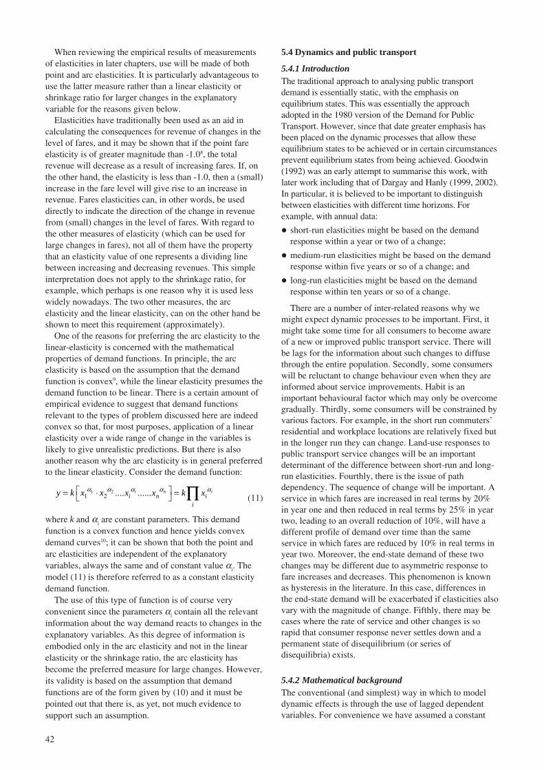
42

When reviewing the empirical results of measurementsof elasticities in later chapters, use will be made of bothpoint and arc elasticities. It is particularly advantageous touse the latter measure rather than a linear elasticity orshrinkage ratio for larger changes in the explanatoryvariable for the reasons given below.

Elasticities have traditionally been used as an aid incalculating the consequences for revenue of changes in thelevel of fares, and it may be shown that if the point fareelasticity is of greater magnitude than -1.08, the totalrevenue will decrease as a result of increasing fares. If, onthe other hand, the elasticity is less than -1.0, then a (small)increase in the fare level will give rise to an increase inrevenue. Fares elasticities can, in other words, be useddirectly to indicate the direction of the change in revenuefrom (small) changes in the level of fares. With regard tothe other measures of elasticity (which can be used forlarge changes in fares), not all of them have the propertythat an elasticity value of one represents a dividing linebetween increasing and decreasing revenues. This simpleinterpretation does not apply to the shrinkage ratio, forexample, which perhaps is one reason why it is used lesswidely nowadays. The two other measures, the arcelasticity and the linear elasticity, can on the other hand beshown to meet this requirement (approximately).

One of the reasons for preferring the arc elasticity to thelinear-elasticity is concerned with the mathematicalproperties of demand functions. In principle, the arcelasticity is based on the assumption that the demandfunction is convex9, while the linear elasticity presumes thedemand function to be linear. There is a certain amount ofempirical evidence to suggest that demand functionsrelevant to the types of problem discussed here are indeedconvex so that, for most purposes, application of a linearelasticity over a wide range of change in the variables islikely to give unrealistic predictions. But there is alsoanother reason why the arc elasticity is in general preferredto the linear elasticity. Consider the demand function:

1 21 2 .... ......i n i

i n ii

y k x x x x k xα α αα α⎡ ⎤= ⋅ =⎣ ⎦ ∏ (11)

where k and αi are constant parameters. This demand

function is a convex function and hence yields convexdemand curves10; it can be shown that both the point andarc elasticities are independent of the explanatoryvariables, always the same and of constant value α

i. The

model (11) is therefore referred to as a constant elasticitydemand function.

The use of this type of function is of course veryconvenient since the parameters α

i contain all the relevant

information about the way demand reacts to changes in theexplanatory variables. As this degree of information isembodied only in the arc elasticity and not in the linearelasticity or the shrinkage ratio, the arc elasticity hasbecome the preferred measure for large changes. However,its validity is based on the assumption that demandfunctions are of the form given by (10) and it must bepointed out that there is, as yet, not much evidence tosupport such an assumption.

5.4 Dynamics and public transport

5.4.1 IntroductionThe traditional approach to analysing public transportdemand is essentially static, with the emphasis onequilibrium states. This was essentially the approachadopted in the 1980 version of the Demand for PublicTransport. However, since that date greater emphasis hasbeen placed on the dynamic processes that allow theseequilibrium states to be achieved or in certain circumstancesprevent equilibrium states from being achieved. Goodwin(1992) was an early attempt to summarise this work, withlater work including that of Dargay and Hanly (1999, 2002).In particular, it is believed to be important to distinguishbetween elasticities with different time horizons. Forexample, with annual data:

� short-run elasticities might be based on the demandresponse within a year or two of a change;

� medium-run elasticities might be based on the demandresponse within five years or so of a change; and

� long-run elasticities might be based on the demandresponse within ten years or so of a change.

There are a number of inter-related reasons why wemight expect dynamic processes to be important. First, itmight take some time for all consumers to become awareof a new or improved public transport service. There willbe lags for the information about such changes to diffusethrough the entire population. Secondly, some consumerswill be reluctant to change behaviour even when they areinformed about service improvements. Habit is animportant behavioural factor which may only be overcomegradually. Thirdly, some consumers will be constrained byvarious factors. For example, in the short run commuters’residential and workplace locations are relatively fixed butin the longer run they can change. Land-use responses topublic transport service changes will be an importantdeterminant of the difference between short-run and long-run elasticities. Fourthly, there is the issue of pathdependency. The sequence of change will be important. Aservice in which fares are increased in real terms by 20%in year one and then reduced in real terms by 25% in yeartwo, leading to an overall reduction of 10%, will have adifferent profile of demand over time than the sameservice in which fares are reduced by 10% in real terms inyear two. Moreover, the end-state demand of these twochanges may be different due to asymmetric response tofare increases and decreases. This phenomenon is knownas hysteresis in the literature. In this case, differences inthe end-state demand will be exacerbated if elasticities alsovary with the magnitude of change. Fifthly, there may becases where the rate of service and other changes is sorapid that consumer response never settles down and apermanent state of disequilibrium (or series ofdisequilibria) exists.

5.4.2 Mathematical backgroundThe conventional (and simplest) way in which to modeldynamic effects is through the use of lagged dependentvariables. For convenience we have assumed a constant

43

elasticity formulation but variable elasticity versions canbe devised. The constant elasticity formulation involvesestimation of an equation of the following form:

1it jt it itV F Z Vβ γ δα −= (12)

where:

Vit

= Volume of public transport travel in area i intime period t.

Fit

= Mean public transport fare in area i in timeperiod t.

Zit = Vector of other relevant explanatory variables.

Vit-1

= Volume of public transport travel in area i intime period t - 1.

α, β, γ, δ are parameters to be estimated.

With this formulation, the short run fares elasticity isgiven by the parameter β and the long run fares elasticity byβ / (1 - δδδδδ). The medium run fares elasticity is more difficultto estimate. To do so, it becomes helpful to re-write theabove equation in logarithms:

it it it itlnV ln ln F lnZ lnVα β γ δ= + + + (13)

If we let V*i be the equilibrium value of Vi, let Xt be thedeviation of ln V

it from ln V*i and let X

0 be the difference

between ln Vi0 (the starting value) and ln V*i, we can

determine that:

t oX tXδ=

Suppose we have estimated a short run elasticity of -0.4and a long run elasticity of -0.8 from annual data coveringyears 1 to 10 with a major fare change at the beginning ofyear 1, this would imply a value of δ equal to 0.5. Supposealso that the fare change at the beginning of year 1 hadbeen a 20% increase. We would be forecasting a 13.6%decrease at the end of year 10 and a 7.0% decrease at theend of year 1. We can then calculate that:

ln Vi1 – ln (0.864) = 0.5 (ln (1) – ln (0.864)) and hence

Vi1

= 0.930. (demand down by 7.0%).

ln Vi5 – ln (0.864) = 0.55 (ln (1) – ln (0.864)) and hence

Vi5

= 0.868. (demand down by 13.2%).

ln Vi10

– ln (0.864) = 0.510 (ln (1) – ln (0.864)) and henceV

i5 = 0.864. (demand down by 13.6%).

In this example the change occurs relatively quickly.51% of the change occurs by the end of year one and 97%of the change by the end of year five. The implied mediumrun five year elasticity is -0.78.

This is an example of a partial adjustment model. In thiscase, the higher the δ estimate, the slower the speed ofadjustment and the greater the difference between the shortrun and long run elasticities. The number of periods nrequired to close a given proportion p of the gap between theequilibrium and starting values of V can be calculated as:

( ) ( )1 /n ln p ln δ= − (14)

There are a number of different ways in which dynamicsmay be incorporated including specifying lags of higher orderthan the first order lag presented above and including lagged

independent variables. Partial adjustment models of this typehave been criticised for using short time-series and forignoring the fact that data are non stationary (i.e. thatvariables tend to grow (or in some cases reduce) over time).There may be spurious correlations between variablesexhibiting random walks. This can lead to statistical problemswith goodness of fit measures meaning that incorrectinferences might be drawn. More advanced econometrictechniques, such as co-integration and error correctionmodels, have been developed to overcome some of theseproblems. However, error correction models can be more dataintensive and hence partial adjustment models are often usedwhere time series data sets are limited in duration.

The simplest error correction models use an Engle-Granger two-step estimation procedure. This involvesestimating a long-run relationship from a static regression:

it it itV Fβ µ= + (15)

where β is the long run fare parameter (if logs are taken thiswill be the long run elasticity) and µ is the stochastic errorterm. The stationarity of µ is then examined using tests suchas the Durbin–Watson test of the cointegrating regression. Ifco-integration is indicated (that is that the variables in levelsare non stationary but some linear combination – in this casefirst differences – is stationary), the residuals from the co-integration regression µ are used as an error correction termin a model of the following form:

( ) 11it o it itV Fβ ϕ µ −∆ = ∆ + − (16)

It should be noted that in the error correction model thevariables are specified in terms of differences (denoted by∆) rather than levels. The short run fare parameter is givenby β

0 (this will be the short run elasticity if logs are taken)

and the feedback effect is given by (ϕ - 1). This indicatesthat (1 - ϕ) of the deviation between the short-run andlong-run response is closed each period.

5.4.3 ExamplesBusDargay and Hanly (1999) provide some usefulcomparisons of the two approaches, at least for the Englishmetropolitan areas (excluding London). A partialadjustment model estimates a short run fare elasticity of-0.74 and a long run elasticity of -1.09. The moreappropriate error correction model (given that the datawere found to be non stationary) estimates a short run fareelasticity of -0.69 and a long run elasticity of -1.06. For theerror correction model (ϕ - 1) was estimated at -0.68suggesting a relatively quick adjustment (68% of changeoccurring in the first time period). This is identical to thefindings from the partial adjustment model, given a valueof δ of 0.32, which implies 68% of change (1 - δ) occurs inthe first time period.

This suggests that the use of the partial adjustmentmodel, in this case, does not lead to any serious biases inestimation. However, there were larger differencesbetween the estimated elasticities from the error correctionmodel and the partial adjustment model when separateestimates were made for each of the six Englishmetropolitan areas (see Table 5.1).

44

This suggests that there is the need for furthereconometric work to test the robustness of the errorcorrection and the partial adjustment methods. There mayalso be scope for investigating error correction/cointegration models that involve higher than first orderdifferences. Other issues include the assumption that allexplanatory variables are exogenous (if this is not thecase a system of equations needs to be estimated) and,where there are more than two variables, that there isonly one cointegrating relationship. Both theseassumptions need to be tested.

The above discussion also assumes that the demandmodels are fully specified. These models included servicelevels and income as explanatory variables in addition tofares but they do not include measures of bus speeds. Itmight be expected that bus speeds have decreased overtime and that these decreases might be correlated with theincreases in fares (estimated to have gone up by between23% and 202% between 1985 and 1996 for the six areasstudied). This might have led to biases in the estimationof the fare parameter values and, if decreases in busspeeds have become more marked over time, might haveled to the erroneous detection of a long-run effect. Otherexplanatory variables missing from the analysis includethe price (and other attributes) of rival modes,particularly rail-based public transport and the privatecar, and the overall composition of the market (includingthe importance of concessionary groups such as theelderly). It should be noted that the elasticities for theMetropolitan areas are higher (in absolute terms) thanthose recommended by Goodwin and Dargay (2001) forGreat Britain as a whole (where motoring costs andproportions of pensioners are also included asexplanatory variables). They suggested a bus fareelasticity of around -0.4 after one year, -0.6 after two

years, -0.8 after five years and –0.9 after ten years. As theestimates are based on a partial adjustment model, thisimplies a value of δ of 0.56, with 44% of changeoccurring in the first period. Models of this type suggesta short and long run fare elasticity for the Shire countiesof -0.49 and -0.66, with the corresponding elasticityestimates for the Metropolitan areas being -0.26 and -0.54 (Dargay and Hanly, 2002). However, it should benoted that these estimates are constrained to produce thesame elasticities across areas of a similar type and arethought to be less appropriate than area specificestimates. Nonetheless, it suggests that results may besensitive to the level of spatial aggregation.

Two other applications of error correction models to theBritish bus industry are the studies undertaken by Romilly(2000) and by OXERA (2003). Romilly’s study was basedon annual data for the British bus industry outside London1953-1997. The OXERA study used data for theGovernment Office Regions (excluding London andNorthern Ireland) between 1985/6 and 1999/2000.

The results are given by Table 5.2. In the Romilly modelthe feedback parameter (ϕ - 1) was estimated at -0.37, butthe OXERA study did not report the feedback parameters,which, unlike Romilly vary across the attributes of interest.For comparison, the Dargay and Hanly (1999)recommended values are also given. There is someconcurrence between these three studies with respect to thelong-run bus fare elasticity but important differences withrespect to all other estimates, particularly income. Thisreflects the sensitivity of error correction methods to dataand model specification, as well as the sensitivity to spatialaggregation noted above which is also reflected by theinstability of OXERA’s results at the Government OfficeRegion level.

Rail

An example of a partial adjustment model of rail demandis the work of Owen and Phillips (1987) whose initialwork was based on four weekly ticket sales data for 20Inter City routes from 1973 to mid 1984. There were 149time series observations per route. Their median resultssuggested a short term price elasticity (i.e. after onemonth) of -0.69, whilst the long term elasticity was -1.08.This suggests an estimated median value of δ of 0.36. Wecan use this to rework our earlier analysis although we arenow forecasting that a 20% fare increase at the start of theperiod would result in a 17.9% reduction in demand by theend of the period.

Table 5.1 Comparison of fare elasticities from an errorcorrection model and a partial adjustmentmodel for six english metropolitan areas

Error correction model Partial adjustment model

Short run Long run Short run Long run

Manchester -0.35 -0.96 -0.79 -1.09Merseyside n.s. -0.70 -0.52 -0.72South Yorks. -1.13 -1.08 -0.82 -1.13West Yorks. -0.90 -1.22 -0.85 -1.17Tyne & Wear -0.73 -0.70 -0.59 -0.81West Midlands n.s. -1.11 -0.82 -1.13

n.s. = not significant at the 10% level

Table 5.2 Error correction model estimates of bus demand elasticities

Bus fare elasticity Bus service elasticity Income elasticity Car price cross-elasticity

Study SR LR SR LR SR LR SR LR

Romilly (2000) -0.38 -1.03 0.11 0.30 0.23 0.61 0.17 0.45OXERA (2003 -0.63 -1.08 0.38 0.37 0.60 -0.56Dargay and Hanly (1999) -0.4 -0.9 0.4 0.9 0 -0.5 to -1.0 0 0.3 to 0.4

SR – short run; LR = long run

45

ln Vij2


ij2 = 0.842. (demand down by 15.8%).

ln Vij3


ij3 = 0.829. (demand down by 17.1%).

ln Vij6


ij6 = 0.821. (demand down by 17.9%).

In other words, this modelled example suggests thatvirtually all of the change occurred within the first sixmonths. Indeed, 66% of change occurred by the end of thefirst month, 88% of change by the end of the secondmonth and 96% of change by the end of the third month.This might lead one to conclude that dynamics are not thatimportant for long established Inter City routes.

One important point to note here is that Owen andPhillips worked with (broadly) monthly data whilst Dargayand colleagues worked with annual data. There is somescope for econometric work that tests whether differenttypes of data with respect to time period tend to exhibitdifferent dynamic effects.

An alternative way that long term demand increasesmight be forecast is through the use of models that forecastthe impact transport improvements might have on landuse, particularly residential and workplace location. Anexample of such a model is the Leeds Integrated Land Useand Transport (LILT) model developed by Mackett andBird (1989) and applied to Network South East in the late1980s This model worked in increments of five years froma base year of 1986. Some elasticity estimates arepresented in Table 5.3.

From Table 5.3 it can be seen that the estimated short runtravel time elasticities are around 90% of the long-runvalues. For fare, the short-run elasticities are between 60%and 90% of the long-run values. However, in the case offare elasticities, this is not just due to land use changes butalso because rail fares increase over time. LILT isunderpinned by a logit model in which (absolute) elasticitiesincrease with the value of the attribute of interest (in thiscase rail fares). Hence the long run impact on the elasticityvalue of a 5% per annum fare increase is more marked thanthe impact of a 1.5% per annum fare increase.

5.4.4 ConclusionsThere is an increasing amount of evidence on the dynamicprocesses that underpin public transport demand butknowledge remains limited. In part, this is due to the

limited availability of consistent data sets that cover longtime periods. It is also due to problems with estimationmethodologies. However, what evidence there is suggeststhat demand for the local bus industry which might take 10years for demand to fully respond to fare and servicechanges, with long run elasticities two to three times theshort run elasticities. In contrast, demand for longestablished Inter City rail routes seems to respond quicklyto marginal changes in fares and, by inference, services.This apparent discrepancy between the dynamic propertiesof bus and rail demand requires explanation. There is someevidence that the long term impacts of fare and servicechanges may be more important for commuter railservices, where land use impacts may be more importantthan for inter-urban transport. This may provide a partialexplanation of the discrepancy between bus and rail. Thereis also some evidence that the demand for new (ordramatically improved) rail products takes time to emerge(ATOC, 2002). For new high speed rail services, it maytake up to four years for demand to reach an equilibrium,with demand in year one only around 50% of that in yearfour. For new urban rail services, it may take slightlylonger (five years) for demand to reach an equilibrium, butgrowth will be less marked, with demand in year one being75% of that in year five. It is important to take thesedemand build-ups into account when appraising new orimproved public transport products.

5.5 Effects of demand interactions

Where there are competing forms of transport, a change inthe price or other attributes of one may affect demand foranother. Such demand interactions are known as crosseffects. We distinguish between two types of cross effect:that emanating from the competition between modes andthat emanating from competition within modes. The keyindicator is the cross-elasticity which, for a price change,may be expressed as follows:

jiij

j i

PQ

P Qη ∂

=∂ (18)

where:

ηij

= the cross-elasticity of demand for service i withrespect to the price of service j,

Qi

= the demand for service i, and

Pj

= the price of service j.

Table 5.3 Short run, medium run and long run elasticity estimates from LILT

All trips Trips to central London

Short-run Medium-run Long-run Short-run Medium-run Long-runChange modelled (1991) (1996) (2001) (1991) (1996) (2001)

Fares increased by 1.5% per annum1 -0.31 -0.32 -0.35 -0.15 -0.17 -0.19Fares increased by 5.0% per annum2 -0.33 -0.38 -0.45 -0.17 -0.22 -0.28Travel times reduced by 10%3 -0.63 -0.67 -0.69 -0.34 -0.36 -0.38

1 First fare increase implemented in 1991 (fares up 7.73%), subsequently fares increased by the same percentage in 1996 and 2001. (Test 1A).2 First fare increase implemented in 1991 (fares up 27.63%), subsequently fares increased by the same percentage in 1996 and 2001. (Test 1B).3 Central London rail times (including Underground) remain constant. Many rail journeys include travel within central London, so the actual average

reduction was less than 10% and the travel time elasticities are slight under estimates. (Test 2C).

46

In practice such effects may be difficult to measurebecause the direct effects (e.g. of the change in P

i on Q

i)

often outweigh the cross effects (e.g. of the change in Pj on

Qi). However, we can infer cross-elasticities from direct

elasticities by making use of the following formula:

jiij ii

j i

QQ

Q Qη η

∂=

∂ (19)

where

ηii

= the direct elasticity of demand for service iwith respect to the price of service i (alsoreferred to as own price elasticity).

Qi /Q

j = the relative market volumes of services i

and j.

∂Qj /∂Q

i= the proportion of the change in service i trips

as a result of a price change that are divertedfrom mode j. We refer to this as a diversionfactor and will present some evidence onsuch factors below.

Cross-elasticities have some other theoretical propertiesthat can be useful. We highlight briefly two. First, there isthe homogeneity condition. This simply states that for anygood the sum of the own-price elasticities and all cross-priceelasticities equals minus the income elasticity. Secondly,there is the symmetry condition which, assuming no incomeeffects, states that for all i not equal to j:

ji

j i

QQ

P P

∂∂=

∂ ∂ (20)

These two conditions can be used to infer a full set ofcross-elasticities in situations where only a sub-set ofdirect and cross-elasticities are known. This assumption ofthere being no income effect implies that the elasticity ofdemand for a service with respect to income is zero and/orthe proportion of income spent on a service is zero. Inmany circumstances in public transport markets this maybe an adequate approximation of the truth.

5.6 The ratio of elasticities approach

Mode A’s own fare elasticity for user group 1 (e.g.commuters) in circumstances where multiple travelchoices exist and when these choices are described by thelogit function is given by:

( )1 1 1 11 ProbA AE b C= − (21)

Where:

b1

is the cost parameter;

C1

is the cost;

ProbA1

is the probability of choosing mode A.

The ratio of elasticities can be used in solving therelationship between aggregate elasticities anddisaggregate elasticities. The ratio between user group 1and user group 2 elasticities is given by:

( ) ( )1 2 1 1 1 2 2 2/ 1 Prob / 1 ProbA A A AE E b C b C= − − (22)

This relationship can be simplified, if:

� The relationship between C1 and C

2 is known (e.g. the

stage fare is 50% lower for one group and similarjourney lengths are undertaken).

� BUT MORE IMPORTANTLY: Mode A has the samemarket share for user groups 1 and 2.

More generally, suppose we can write price elasticity asfollows:

( ) ( )/ /pE Q P P Q= ∂ ∂ ⋅ (23)

where:

Q = Volume of bus travel,

P = Mean bus fare.

Suppose also we can express value of time as follows:

( ) ( )/ / /VoT A T Q P= ∂ ∂ ∂ ∂ (24)

where:

T = Mean bus in-vehicle time.

Then we can write in-vehicle time as follows:

( ) ( )/ /TE q T T Q= ∂ ∂ ⋅

( ) ( ) ( ) ( ) ( )/ / / / /Q P P Q Q T P Q T P= ∂ ∂ ⋅ ⋅ ∂ ∂ ⋅ ∂ ∂ ⋅

/pE VoT P= ⋅ (25)

In other words, if we have reliable estimates of the priceelasticity and the value of in-vehicle time, then we caninfer the in-vehicle time elasticity for any combination ofin-vehicle time (T) and fare (P).

5.7 An example of the use of elasticities

One important use of elasticities in public transportplanning is, as mentioned above, to indicate the directionand size of the change in revenues from changes in thelevel of fares. More recently elasticities have becomeimportant in other areas and in particular when consideringthe supply of public transport services. The use ofelasticities for this purpose will be indicated below using asimple hypothetical example.

An average journey by bus in a particular urban areainvolves 8 minutes waiting time, 10 minutes walking timeand 12 minutes in-vehicle time. A service increase, limitedby a fixed budget, is planned for the network. Within thisbudget constraint the following three strategies arefeasible:

a A decrease in bus headways which would reduce theaverage waiting time from 8 to 5 minutes.

b An increase in the number of routes which would reducethe average walking time from 10 to 6 minutes.

c An extension of reserved bus lanes and bus-only roadswhich would reduce the average in-vehicle time from 12to 10 minutes.

If it is assumed that the arc elasticities with respect towaiting time (wt), walking time (st) and in-vehicle time(vt) are:

47

earcwt

= -0.5.

earcst = -0.6.

earcvt

= -0.4.

then it is possible to calculate the percentage change inpatronage for each of the three strategies as follows:

a 100 [(5/8)-05 -1] = 26%.

b 100 [(6/10)-0.6 -1] = 36%.

c 100 [(10/12)-0.4 -1] = 8%.

If the aim is to maximise the number of passengerjourneys, the strategy (b) should be chosen.

5.8 Some guidelines on the prqactical use of elasticities

Using elasticities in practice is quite simple, as has beenillustrated above, and this also accounts for their popularity.It must be pointed out, however, that elasticities are notstrictly a substitute for demand functions, except in somespecial cases, since they only convey limited informationabout the structure of demand. When calculating and/orusing elasticities, attention should be paid to the propertiesof the elasticities in order to ensure that their limitations areunderstood and that they are applied only when it is valid todo so. Such properties include:

i The size, direction and type of change.

ii The purpose of the journey.

iii The time period over which the demand is measured.

iv The characteristics of the individuals or sections ofpopulation concerned.

v Transferability in time and space.

vi Whether the effect refers to the short or the long term.

vii The functional form of elasticity used in the originalstudy.

Each of these aspects is considered in more detail asfollows:

i Elasticities are usually calculated at only one or twovalues of the explanatory variables. Since the entiredemand function is not known, elasticities may differ fordifferent types of change and for different initial valuesof the variable being changed. There are other reasons,however, why elasticities depend on the type of changebeing studied; for example, it is often argued that it iseasier to lose passengers than to gain them becauseincreases in fares, or decreases in the supply, inducetravellers to seek alternative means of transport, such ascars; once a car has been bought, the owner tends tobecome ‘captive’ to his vehicle. If this is so, then thefares elasticity might be expected to be larger whenfares are increased than when they are decreased. It isalso suggested that elasticities might be larger for largechanges than for small ones, since large changes areeasier to perceive than small ones and consequentlyinduce a more active search for alternative travel modesor destinations.

ii Elasticities may also be expected to vary with journeypurpose, since they are bound to be dependent to someextent on how optional the particular journey is (at least

in the short term). Elasticities associated with workjourneys are thus in general smaller than thoseassociated with other types of journeys, such asshopping and socialising, since there are usually veryfew substitutes for work journeys (though this may notbe true in the long term). Other types of journeys canoften be made at different times, to different destinationsor by different modes (or omitted altogether, ifnecessary) if travel times and costs are increased, so theresponse is relatively sensitive to such changes, givingrise to correspondingly larger elasticities.

iii An elasticity refers to a response averaged over a givenperiod of time, which may be as short as the rush houror as long as a year or more. The elasticities for differenttime periods will reflect the different types of journeywhich predominate and the alternative modes which areavailable.

iv As noted earlier, demand functions may refer either toindividuals or to groups of individuals. Calculatingelasticities from individual data may be of limited valuesince elasticities are mainly used to determine groupbehaviour. In particular, it is necessary to make sure thatthe values of the explanatory variables used as input toindividual demand functions do represent averages forthe population which the elasticity is supposed to reflect.In many instances this has not been so. The sameproblem applies to aggregate functions also.

v Elasticities are not necessarily transferable in time or inspace. One reason for this is that preferences changeover time. Furthermore, with incomes rising over time itmay be expected that consumers would become morewilling to pay more to avoid discomfort and to reducetravelling time (though see Section 5.2 - the demandfunction concept), which would mean that elasticitieswith respect to travelling times would be expected torise in relation to price elasticities if the money costsinvolved rise less rapidly than income. Similarly,elasticities derived from data obtained in one area maynot be applicable to other areas where car ownership,incomes, the level of public transport service etc may bequite different.

vi A final aspect to which attention should be paid whenusing elasticities is whether they reflect long-run orshort-run behaviour. This is because changes in aparticular aspect of public transport, such as travellingtimes, have both a direct and an indirect impact ondemand, as has been emphasised above. The directimpact is registered shortly after the change, but theindirect impact, which may be due to changes inresidential location or car ownership levels, affectsdemand at a much later date; thus, the full effects of,say, a fare change may not be realised for several years.Whether a demand function and the elasticitiescalculated from it reflect short- or long-run effects inthis sense is a consequence of both the type of modelused and the type of data employed to estimate thedemand function. Even if it is only required to knowabout the short-run effects on demand from a change inan explanatory variable, it is not always possible to

48

observe the effects until some time has elapsed; forexample, it is a common experience that full adjustmentsto a fare change may take as long as six months, partlybecause it takes passengers some considerable time tofind acceptable alternatives and settle into new travelhabits, but also because a fare increase is often followedby a short-lived passenger ‘protest’ which depressesdemand abnormally. As a consequence, elasticities whichare calculated from observations made soon after a fareincrease may be larger than those based on observationsmade rather later, if the ‘protest’ effect dominates, or thereverse may be true if demand is taking some time tosettle down.

viii As indicated in earlier parts of this chapter, thefunctional form of the elasticity used in the originalreference study may have substantial effects on thevalues derived. It is therefore desirable to useelasticities in the same functional form as that in whichthey were initially estimated, although this may notalways be possible in practice where the original studyspecification is not readily available.

5.9 Incorporation of revealed preferences changes notreflect in 'elasticity' values

Many of the principal demand factors can be represented innumerical form, to which appropriate elasticity values maythen be related (such as those for fares, and frequency).Changes in demand resulting from changes in such factorsmay then be estimated by inputting the appropriate changesin the causal variable (such as a fares increase). This isrepresented by a shift along a demand curve.

There may be greater difficulty in assessing discrete of‘step’ changes in factors which may not be quantifiable interms of continuous variables. For example, increasedattention has been paid by operators to factors such asmarketing, driver training, improved vehicle design (suchas low-floor access, or air conditioning), alternative farestructures, etc. One method of analysing such changes is toview them as a demand curve shift, i.e. a shift betweendemand curves, or a shift of an existing demand curve tothe left (where the net effect has been to worsen quality ofservice, resulting in lower demand) or the right (where animprovement has occurred, increasing demand).

For example, the severe instability in bus servicesfollowing deregulation in Britain in the mid 1980s couldbe represented as shift of a demand curve to the left (i.e.allowing for changes in average real fare, servicefrequency and exogenous factors, demand was lower thanwould have been expected on established elasticityvalues). Conversely, large increases such as those due toimpacts of an extensive marketing campaign would beseen as a shift of the demand curve to the right.

While less easy to quantify in terms of traditionalestimation methods, such factors may well have greaterimpact on public transport demand than substantial changesin fare or service levels, and may be far more cost-effective,especially in the short term, in which demand with respect tofare or service level is fairly inelastic.

This may also be an appropriate method for looking atshifts occurring through travel awareness campaigns, andpersonalised travel marketing, which can result insubstantial growth in ridership without any changes inservice level or price, especially where the current marketshare of public transport is low, and hence even a smallshift of car travel to public transport represents a largepercentage growth in the public transport demand.

A good example was the pilot scheme carried out inPerth, Western Australia, in 1997, following earlier workby Socialdata in Germany, using ‘soft’ policies toinfluence modal choice (Brög and Grey-Smith, 2002). Theconcept of ‘Individualised Marketing’ was an essentialcomponent of this approach. Households were contacted todetermine their existing modal choices and journeys made,and scope identified for transfer to modes such as walking,cycling and public transport from car. Trips per person perday remained the same before and after the project, at 3.4,but those made as car driver fell from 60% to 54% and bustrips rose from 6% to 7%. This was followed by a larger-scale demonstration project in South Perth, including over13,000 households, producing similar results.

Another recent example is the direct telephone-basedmarketing conducted by Stagecoach in Britain, giving anestimated modal shift from car of up to 9% (Transit, 2003).

It may also be the case that changes occursimultaneously in factors which can be quantified and forwhich elasticity values have been established fromprevious studies, and those more appropriate to thedemand curve shift concept. For example, a revised urbanbus network may be accompanied by changes in vehicle-km operated (as a proxy for frequency) and average fare,together with simplification of routes, changes in farestructures, extensive marketing, etc.

As part of the study, a number of cases have beenidentified where performance has differed substantiallyfrom that generally found in Britain (for example, busridership in certain urban areas, outside London). As ameans of identifying the effect of factors other thanchanges in fare level and service level, data have beenprovided by the operators concerned for changes inridership, average revenue per trip and vehicle-kmoperated. Using representative elasticities for suchvariables, the ‘expected’ and ‘observed’ outcomes may becompared. The difference due to other factors may then beestimated. This has already enabled quantification ofeffects due to marketing and fares simplification. (Note:due to reasons of commercial confidentiality, resultsreported in the study will discuss overall conclusions fromsuch analysis, rather than individual cases in detail).

In terms of converting such demand curve shifts toestimates to changes in consumer surplus, a distinctionneeds to be drawn between two types of shift:

a An improvement in service quality which is notnecessarily reflected in variables for which conventionalelasticity values can be calculated, which results inbenefits both to existing and to new users. Examplesmight include real-time information at stops, low-flooraccess to vehicles, etc.

49

b A growth in demand due to wider awareness of existingservices through personalised travel marketing, etc. Inthis case, while new users may be assumed to enjoysome benefits (otherwise their behaviour would not havechanged), it would not be reasonable to infer similarbenefits for existing users already aware of the serviceoffered.

5.10 Concluding observations

Any modelling of public transport demand must involve aconsiderable degree of simplification. It is always importantto bear in mind that most travel comprises trip chains madeby individuals from the home. Indicators of demand need toallow for effects of definitions used, especially in respect oflinked trips. Aggregate demand changes may result bothfrom existing users changing their level of use, and otherseither joining or leaving the public transport market as aconsequence. For many of the major demand variables, suchas fares and service levels, elasticities may be derived fromobserved data, or stated preference responses. This may bemore difficult to apply directly to factors affectingperception and awareness of services.

6 Effects of fares

6.1 Introduction

In this chapter, the effects of fares on public transportpatronage are considered. Fares are fundamental to theoperation of public transport since they form a majorsource of income to operators. In general, if fares areincreased, patronage will decrease. Whether revenueincreases or decreases as a result of a fare increase dependson the functional relationship between fares and patronageas represented by the demand curve. Usually this isexpressed through the concept of ‘elasticity’ which wasdiscussed in Chapter 5.

Recent research suggests that fare elasticities aredynamic, meaning that they vary over time since the farechange. Therefore, it is increasingly common for analysts todistinguish between short-run and long-run, and sometimesmedium-run elasticity values; there are various definitionsof short-run, medium-run and long-run, but most authorstake short-run to be 1 or 2 years, and long-run to be around12 to 15 (although sometimes as many as 20) years, whilemedium-run is usually around 5 to 7 years.

In recent years, two quite different methods have beenused in econometric studies to distinguish between short-run and long-run elasticities. The first is to define, a priori,certain classes of behavioural models to be interpreted asindicating something about the time scale of the responseas ‘short-term’ or ‘long-term’. In principle, this enablessuch cross-section, or equilibrium, models to be interpretedas indicating something about the time scale of theresponse, by consideration of which responses areincluded. The conditions for this to be valid are stringentand rarely fulfilled, and even where they are, no statementsare possible about how many years it takes for the long-term effect to be completed.

The second approach is to use a dynamic econometricmodel in which time series data are used with a modelspecification in which a gradual response over time isrepresented explicitly. In this case, the short-run is theinterval of the data series; for example, the short-run is oneyear for annual data, three months for quarterly data and soon. The long-run response and its time scale aredetermined empirically as key results of the analysis.

There have been many papers on fare elasticities. Intheir day, two of the most influential, were the 1980‘Demand For Public Transport’ (Webster and Bly,1980)and a report by the Commission of The EuropeanCommittee (1980). More recent major reviews on thesubject, include: Dargay and Hanly (1999), Goodwin(1992), Oum et al. (1992) and Goodwin et al. (1992). Thelatter three are interrelated. The first draws on the lattertrio, but supplements it with more recent work. Accordingto this quartet, other useful literature reviews are: Fowkes,Sherwood and Nash (1992), Oum et al. (1990), Goodwin(1988), and Goodwin (1991).

Elasticities can be derived in a number of ways, forexample: time trends, stated and revealed preferencesurveys, before-and-after studies, time series analysis, cross-sectional analysis, and logit modelling. For more informationon the different types of modelling see Chapter 5. All formsof modelling have their drawbacks: before-and-after studieshave tended to deal with the short-run rather than the long-run, stated preference surveys may be skewed in two ways:firstly, people may react differently in the real situation tohow they think they will react, and secondly, in order toobtain their desired outcome (e.g. a new bus service) theymay say they will react in a particular way when they knowthey will not. Time trends are not always a reliable indicator,as they can be subject to policy change. For example timetrend estimates, as well as including the response to farechanges, may incorporate past changes in car ownershipwhich have been influenced by policy intervention on caruse which have led to increased public transport use, so thatthe resulting elasticity values may appear higher than theyotherwise would be.

In this study, elasticity values from many sources havebeen examined. Some are discussed in the text. Others areincluded in the Appendix to Chapter 6. This shows, foreach study covered, the elasticity value, the nature of thevalue, the source reference and then summarises the valuesby means of averages and standard deviations. Generally,one value is taken from each study for the averagingprocess to avoid bias towards studies which have producedseveral values.

A traveller’s response to a fare change will depend, tosome extent, on how large a part the fare plays in thedecision to make that journey or the choice of mode. Forexample, journeys to work or school are necessary, at leastin the short-term. In the longer term, people may changetheir location, and their individual circumstances willprobably change anyway, due to changes in age, income,educational status, employment situation, family situationand so on. All of these factors have an influence onwhether people make a particular journey, by a particularmode. People may travel at particular times of the day to

50

take advantage of the various fare reduction optionsavailable at that time, or use pre-paid discount cards forparticular types of people or groups (such as young peopleor families) to obtain a reduced fare. More work isrequired on how this affects elasticity (Wardman, 1995).There is some evidence of passengers changing ticket typerather than mode in response to a fare increase (SteerDavies Gleave,1999a). This reflects the context-specificnature of some ticket types.

As well as considering the direct effects of a change infares, it is important to consider the effects of fare changeson other modes. The usual method to take into account theeffect that other modes have on the demand for a particularmode of public transport is to use cross-elasticities. Theseestimate the demand elasticity for a competing mode withrespect to the change in the given mode, e.g. the demandelasticity of bus travel with respect to rail fares. They willbe discussed in Chapter 9.

The rest of this chapter synthesises evidence to providean up-to-date overview of fares elasticities and the effectsof various factors on the values.

6.2 Types of fares

Fare systems can have various forms; for example, theycan be flat, zonal or graduated. Each of these has itsparticular characteristics (White, 1995):

Flat fare - A single fare paid regardless of distancetravelled.

Zonal fare - A flat fare applies for travel within adesignated zone.

Graduated fare - A fare charged by distance or a farecharged which varies with costs and loadings.

Season ticket - Weekly, monthly or annual season ticketswhich offer discounts off individual trip tickets and canresult in large savings for the passenger.

Travelcard – A card allowing unlimited use of publictransport within a specified area over a fixed time period(eg one day or one week). It may apply to all publictransport services, or be limited to particular modes oroperators. It may be purchased at ticket offices, automaticticket machines etc. The name ‘travelcard’ is used inLondon; others may be used elsewhere.

For more details on the various types of fares see theAppendix to Section 6.2.

As discussed above, there are many types of fare. Forthe purposes of analysis, it is often necessary to define asingle value, which will often be the average amount paidfor a single trip. This can be calculated by summing all thepassenger receipts in the market segment of interest anddividing by the equivalent number of passengers.Alternatively, the total revenue might include fundingreceived to compensate for concessionary fares that theoperator offers as part of a policy agreement.

6.3 Elasticity of bus travel

In this section, the response of demand to changes in busfares are discussed, including a discussion on short,medium-run and long-run elasticity values.

Table 6.1 shows the average value for bus fare elasticity,averaged over the 49 studies identified in the Appendix toChapter 6. It can be seen that the overall short run bus fareelasticities average about -0.41, which is considerablyhigher than the -0.30 given in the 1980 report (Websterand Bly, 1980). It has been found that in the short run theUK data for bus fare elasticity averages around -0.42,however, the international data have a lower averageelasticity of around -0.38. This difference may reflecthigher fare levels and lower service levels in the UK thanelsewhere in the world.

Table 6.1 Bus fare elasticities (short-run values)

Location Elasticity Number of values

UK -0.42 33Non-UK -0.38 11Overall -0.41 44

For data and sources see appendix to Section 6.3, Tables A6.3 and A6.7.

Table 6.2 Bus fare elasticities related to time period

Average Standard NumberSource Time period elasticity deviation of cases

Before and after studies Around 6 months -0.21 0.12 3Explicit short 0-6 months -0.28 0.13 8Unlagged time series 0-12 months -0.37 0.18 24Explicit long 4+ years -0.55 0.20 8Equilibrium models 5-30 years -0.65 0.18 7

Source: Goodwin (1992)

Table 6.3 Bus fare elasticities for full-fare payingpassengers

Short run Long run

Great Britain -0.2 to –0.3 -0.7 to –0.9

Source: Dargay and Hanly (1999).

Comparisons with earlier literature reviews, from about1980, show that overall short run bus fare elasticityvalues have increased. This reflects increasing carownership and less reliance on the bus over time. Broadlyspeaking, the results compare closely to those from theearly 1990s (Goodwin, 1992, Goodwin et al., 1992, andOum et al., 1992).

Goodwin (1992) examined the literature to see theeffects of the length of time since the fare change on theelasticity value. His results are shown in Table 6.2.

Goodwin (1992) states that the average of the values inTable 6.2 is -0.41. The mean of the elasticities for thestudies that use a time period of 12 months or less is -0.34.The effect after about four years is about –0.55,which increases over time to about -0.65. More recentwork by Dargay and Hanly (1999) using estimates fromdynamic models produces the figures shown in Table 6.3.These are market elasticities, that is, they reflect the effecton bus patronage of average fare changes of all services ina given area. The long-run values are clearly higher thanthe short-run values.

51

An interesting result was produced by Gilbert andJalilian (1991) using complex econometric models on datafor London. They obtained a value of -0.839 for the shortrun and -1.318 for the long run. (Imposing long-runsymmetry reduced the values to -0.788 and -1.185respectively). The long-run value of greater than unityimplies that revenue would decrease when fares wereincreased. Thus, these suggests that in the short-run, a fareincrease would lead to an increase in revenue, but with thepassing of time, the loss of passengers would be so greatthat this effect would outweigh the increase in the meanfare paid by those still travelling.

Table 6.4 shows the mean elasticity values for the short,medium and long runs, based on UK data. The short-runvalue of -0.42 is the mean of 33 UK studies, as discussedabove. Medium-run bus fare elasticities appear to averagesomewhere between -0.5 and -0.6, which are very similar tothose found by Goodwin (1992) and Halcrow Fox et al.(1993). However, this is based on the results of only twostudies, namely: McKenzie and Goodwin (1986) and Preston(1998), and so caution is required when using this figure.

leave the market (due to changes in their circumstances)and new people enter it. These new people will havedifferent characteristics from the users they replace. Theymay have grown up in a generation, or with a lifestyle,which makes them perceive using public transport as moreor less desirable than the users they replace.

The long-run elasticity is around three times that of theshort run elasticity. This is supported by evidence byDargay and Hanly (1999) who found results for Britishsystems of long-run elasticities for British systems ofbetween 1.5 to 3 times the short-run values.

Dargay and Hanly (1999) asked various bus operators ifthey thought their elasticity estimates were accurate. Theyfound that 77% of those surveyed thought their short-runelasticities were about right, but only 41% thought that thelong-run elasticity was about right; 28% felt it was toohigh, the remainder felt it was too low. 53% of thosesurveyed felt that the elasticity values represented theeffects of fare-change on the market over time accurately,and 39% felt the effects of fare change on individualoperators was represented accurately. Of those surveyed44% made use of elasticity estimates and 52% did not (theremaining 4% did not respond).

6.4 Elasticity of rail travel

6.4.1 Rail elasticities overallIn this section, elasticities for rail travel are considered.Table 6.5 shows that the overall average value is -0.41.This is similar to the value for buses, shown in Table 6.1.As with buses, the UK value is greater than that for the restof the world, but the differential is greater than for buses.

Table 6.4 Bus fare elasticities (UK values)

Length of forecast period Elasticity Number of values

Short run -0.42 33Medium run -0.56 2Long run -1.01 3

For data and sources see appendix to Section 6.3, Tables A6.3, A6.10and A6.13.

Table 6.5 Rail fare elasticities (short-run values)


UK -0.46 35Non-UK -0.33 20Overall -0.41 55

For data and sources see appendix to Section 6.4, Tables A6.16, A6.19,A6.25 and A6.28.

Lon-run bus fare elasticities seem to average around -1,which is noticeably higher than those found in previousliterature reviews, most of which produced values in therange of -0.57 to -0.80. This may be partly due to the currentresults being dominated by cross-sectional modelling, whichtends to produce higher values than other methods (seeSection 6.5), whereas the earlier literature reviews appear tobe dominated by conditional elasticities.

It has been shown that the longer the period over whichthe elasticity values have been calculated, the greater themagnitude of the value. Two reasons can be identified forthis effect. Firstly, it reflects the fact that the longer theelapsed time after a fare increase, the greater the range ofresponses open to those who have been directly affectedby the fare increase. In the short run, bus passengers can,in many cases, switch modes or cease making trips. In thelong run, they can change homes, change jobs, buy cars,and so on. It should be noted that these long-run effects arenot necessarily caused directly by the bus fare increase:these types of decisions are made, typically, every fewyears, and the resultant outcome (where to live, where towork, and so on), will reflect the conditions at the time,including bus fares for those who travel by bus. Withhigher fares, more people are likely to choose locationswhich do not require use of the bus. The second reasonthat long-run values are higher is that, in the long run,there is market turnover: the group of people who usepublic transport in a given area will change as some people

The fare elasticity for rail travel as a whole has a widerange, as shown in the Appendix. This is due in part to thewide variation in the effect of competing modes. Oum et al.,(1992) note that intracity rail travel is likely to besignificantly affected by competing modes, such as bus;therefore cross-elasticities tend to be significant in thiscontext. A considerable amount of work has been done oncross-elasticities, involving rail demand. Of particular noteare Wardman (1997a) and Wardman (1997b) cited in SteerDavies Gleave (1999a), which review choice models andapplications of cross-elasticities for both price and service,between one mode and another, for urban and inter-urbantravel in Great Britain, but acknowledge that results are notnecessarily transferable from area to area. Cross elasticitieswill be discussed in more detail in Chapter 9.

Owen and Phillips (1987), in their work on inter-city railfares, mention how, while in the short run revenue mightbe increased by increasing the price of tickets, in the long

52

term this benefit is quickly eroded by a decrease inpatronage. Wardman (1995), also found that if car costsincreased, then people would be more likely to switch tothe train than the bus, while if car costs decreased morepeople would switch from the train than the bus.

As Table 6.6 shows, there is an increase in the elasticityvalue with time since the fare increase. The differentialappears not to be as great as that for buses, but there are onlytwo values for the long run (and none for the medium run). Goulcher (1990) estimated a short-run elasticity for the

London Underground of -0.43, and a long-run value of -0.61. Gilbert and Jalilian (1991) estimated equivalentvalues of -0.355 and -0.688 respectively for the samesystem (-0.396 and -0.983 respectively with long-runsymmetry imposed in the model). Slightly earlier work byFairhurst et al. (1987) using time series analysis data from1970 to 1985 produced a short run value, after one year, of-0.2 and a longer term effect of -0.4. This all implies thatthe long run elasticity for the London Underground isbetween 1.5 and 2 times the short run value, possiblyhigher. In general the long run fare elasticity appears to bearound twice that of the short run.

Comparisons with other literature reviews arecomplicated by the fact that few of them list metro as aseparate entity. Halcrow Fox et al. (1993) did cover metroseparately and concluded with a short run fare elasticity of-0.40, and a long run value of -0.69.

There appear to be very little data on medium run metrofare elasticities, although Halcrow Fox et al. (1993) literaturereview gives a value of -0.45 for London Underground.

6.4.3 Suburban railThe suburban rail fare elasticities are shown in Table 6.9.

These are equivalent to those for overall rail fareelasticities in Table 6.5.

Table 6.6 Rail fare elasticities (UK values)


Short run -0.46 35Long run -0.65 2

For data and sources see appendix to Section 6.4, Tables A6.16, A6.21and A6.25.

Table 6.7 Metro fare elasticities (short-run values)


UK -0.30 15Non-UK -0.29 9Overall -0.29 24


Table 6.8 Metro fare elasticities (UK values)


Short run -0.30 15Long run -0.65 2


Table 6.9 Suburban rail fare elasticities (short-run values)


UK -0.58 20Non-UK -0.37 11Overall -0.50 31

For data and sources see appendix to Section 6.4,Tables A6.25 and A6.28.

Further information on rail elasticities can be found,according to Goodwin (1992), in Fowkes et al. (1985),Glaister (1983), Hughes (1980), Jones and Nichols (1983),Kroes and Sheldon (1985), Mackett (1985), and Oldfieldand Tyler (1981). Of particular note are Godward (1984)and Bamford (1984) which deal with the West Midlands,and, Hensher and Bullock (1979) and Hensher and Smith(1986) which refer to Australia.

The results in Tables 6.5 and 6.6 include studies of bothmetros and suburban rail. There may be differences in theresponse to changes in fare levels for the two types ofsystem reflecting differences in the length and type of tripserved and the competitive modes. Generally, metro tripswill be shorter with bus or walk as competitors, whilesuburban rail trips will tend to be longer often with car as acompetitor. Given that many of the trips will be to work,there may be a lower degree of captivity to suburban rail,with some commuters choosing alternative job locationsaway from the city centre and travelling by car after a fareincrease (Mackett and Nash, 1991). Metros are consideredin Section 6.4.2 and suburban rail in Section 6.4.3.

6.4.2 MetrosAs Table 6.7 shows, the metro elasticity values tend to belower than the overall rail values, with slightly highervalues from the UK than from the rest of the world. Theoverall value of about -0.29 is considerably higher than thevalue of about -0.15 given in Webster and Bly (1980),although within their range of -0.08 to -0.31.

In the long run, metro fare elasticities tend to be higher thanin the short run, as shown in Table 6.8. It should be noted thatall the UK results are from the London Underground.

As Table 6.9 shows, overall, suburban rail has a fareelasticity of around -0.50. This is identical to the valueestablished by Webster and Bly (1980). There is anoticeable difference between the UK and the non-UKresults, with the latter having an average value of -0.37, alittle less than two-thirds of the UK average value of -0.58.Most of the international results come from the US andAustralia, so the difference could be a result of differenturban morphology. A result from Arsenio (2000) fromSpain also yielded a low elasticity, of -0.33. In contrast,Goodwin (1992) shows a higher mean value of -0.79which is an average over 92 studies, but this included awide variety of different types of rail service, not justsuburban rail.

It can be seen that suburban rail has a higher elasticitythan metro and bus, possibly reflecting the longer averagetrip length with car as a competitor.

53

6.4.4 Comparing bus, metro and suburban railTable 6.10 compares short run bus, metro and suburbanrail fare elasticities, and shows the overall mean, averagedacross all modes.

An alternative approach is to use ‘stated preference’ (SP)techniques. These have been developed to help overcomethe problems in forecasting the potential use of a alternativethat does not exist yet. The method involves the presentationof a series of hypothetical questions to a sample of potentialusers. In the questions, the respondents are asked to trade-off between pairs of attributes that might influence theirdemand for public transport.

Elasticity values for three public transport modes havebeen discussed. Some travellers will have a choicebetween these modes: this means that if the fare on one ofthem is increased, but the fares on the others are keptconstant, some travellers will switch to the alternativepublic transport modes. However, if the fares on all publictransport modes are changed simultaneously, there will beless scope for travellers to switch modes. Hence one wouldexpect elasticity values based on a fare change by just onepublic transport mode to be larger than those based on datafrom a fare change by all public transport modes. Theformer are sometimes known as ‘Own elasticities’ and thelatter are sometimes known as ’Conditional elasticities’.

A different approach is to use some form of spatialtransport model to make forecasts of travel demand underdifferent circumstances, for example with and without afare increase and to use the different levels of publictransport demand forecast as the basis of the calculation ofelasticity values. Since the comparisons are made for thesame point in time, under the two assumptions about farelevels, results from this approach are labelled ‘Cross-sectional modelling’.

There is very little published evidence from statedpreference (SP) studies, so most of the results are RP ownelasticities, RP conditional elasticities, and from cross-sectional modelling. Table 6.11 shows mean elasticityvalues for bus, metro and suburban rail for the UK, andTable 6.12 shows the equivalent for outside the UK.Insufficient values based on stated preference research wereavailable to be included. It can be seen that lower elasticityvalues are, in general, obtained for the conditionalelasticities, when the fares on all public transport modes arechanged, than when the fares on only one public transportsub-mode are changed because, in the former case, travellerscan switch to or from another public transport sub-mode.Cross-sectional modelling tends to produce larger elasticityvalues than the other methods shown for the studies fromoutside the UK, but between the two other methods for UKsuburban rail. The small number of studies makes it difficultto form a definite conclusion.

As discussed above, the conditional elasticities, whenfares on all public transport modes are changed, areconsiderably lower than the own elasticities, wherepassengers on the mode with the fare change can switch toor from other public transport modes thereby reducing theimpact of the change. The cross-sectional modellingproduces the largest values for bus and for metro, and avalue which is lower than that for own elasticities forsuburban rail. The own elasticity values are usually basedon before-and-after studies and so include an element oftime trend. Assuming that the majority of values are basedon fare increases rather than fare decreases, because that is

Table 6.10 Public transport elasticities (short run)

Mode UK Non-UK Overall

Bus -0.42 -0.38 -0.42Metro -0.30 -0.29 -0.29Suburban rail -0.58 -0.37 -0.50Overall public transport -0.44 -0.35 -0.41

Data from Tables 6.1, 6.7 and 6.9.

Metro appears to have a lower elasticity than bus (-0.30compared with -0.42 for bus). This reflects metro’s mainadvantage for many trips: it offers a rapid method of travelfrom outer urban areas to the centre for many commuters.Both bus and car suffer from congestion and so cannotcompete for many such trips, and they are too long to bewalked, so many travellers are largely captive unless theychoose to change employment location. That option is notopen to many workers who work in occupations which arecentrally-located and cannot afford to (or choose not to)live close to the city centre. Suburban rail has higheraverage than either bus or metro. This may reflect the factthat many of these trips are commuting trips from outsideurban areas to the city centre and some commuters havethe option of employment outside the main urban area,travelling by car, as discussed above. It should be notedthat in all cases the averages reflect a wide range of valueswhich show considerable overlap.

Pratt et al. (2000) compared bus and rail rapid transit(metro) elasticities for Chicago, New York, San Francisco,London and Paris and found that bus fare elasticities wereabout twice the magnitude of rail rapid transit fare elasticities.

Table 6.10 also shows that elasticity values tend to behigher in the UK than the rest of the world on average.This may reflect higher fare levels and poorer servicequality in Britain than some other parts of the world.

It can also be seen that the overall public transportelasticity appears to be about -0.4, an increase from thevalue of -0.3 identified in the 1980 Demand for PublicTransport Study. This increase reflects the increase in carownership and decrease in dependence on public transportfor many people over the twenty or so years since thatreport was published.

6.5 Effect of methodology

The results here have been estimated using a variety ofmethods. It is possible that elasticity values are a functionof the methodology used to derive them. This issue isconsidered here for the three modes of bus, metro andsuburban rail.

Much analytical work on public transport demand isbased upon the analysis of observed behaviour bytravellers, for example by examining the numberstravelling on a mode before and after a fare change. Thismethod uses ‘revealed preference’ (RP) data.

54

the more usual situation, then it may be that the ownelasticities incorporate an element of secular trend whichin the UK has, historically tended to be a decrease inpatronage. The cross-sectional modelling is based onconsideration of two different scenarios at the same pointin time and so do not include this secular element.

There have been some studies in which the results fromstated preference work has been compared with those fromrevealed preference analysis. Cummings et al. (1989)carried out research in Chicago using both revealed andstated preference techniques. The revealed preference workwas based on a comparison of patronage before and afterthree fare increases in the 1980s, which produced fareelasticities for bus and metro combined of -0.17, -0.59 and -0.27, which have an arithmetic average of -0.34. In 1987Cummings et al. (1989) carried out a stated preferencesurvey in which 6000 questionnaires were distributed at 25employment centres to obtain information about the journeyto work; 1100 were returned. For non-work trips aninterview survey was carried out at activity centres such asshopping malls that attract non-work journeys. The size ofthis survey is not stated. They obtained an average publictransport fares elasticity value of -0.62 for the whole day,which disaggregated into -0.38 for the peak and -0.82 forthe off-peak. However, they felt that these were too high,and so, when aggregating the individual results, they madecorrections to the car availability classification, andestablished values of -0.19 for the peak and -0.44 for theoff-peak, giving an overall mean of -0.33. This can becompared with the overall elasticity from the revealedpreference work for February 1986 of -0.27, which is thedate nearest the stated preference survey. The wide variationin the revealed preference results should be noted.

Preston (1991) used an aggregate simultaneous model toexamine the effects of opening new railway stations in WestYorkshire. From this he estimated rail fare elasticities of -0.83from the log-linear version and -0.65 from the semi-logversion. They had similar levels of goodness-of-fit (R2 of

0.539 for the former and 0.532 for the latter). He then went onto estimate a disaggregate model in which a hierarchical logitmodel was used for work trips only. It gave an elasticity of-0.34. He then went on to estimate some elasticity valuesfrom stated preference data by examining the effects of smallchanges in fares on the forecasts that had been made. Theoverall mean elasticity value produced for rail travellers was-1.75, which is much higher than that produced using therevealed preference data. Preston (1991) argues that thisdifference is related to the low values of time used and thefact that users had an alternative to rail which they werealready using. Also, he argued, stated preference techniquesdo not take into account fully the effects of habit and inertia.

Kroes et al. (1990) used stated preference techniques ina study on Intercity Cross-Country rail services in Britainin 1987. The main objective of the study was to examinethe potential for increasing net revenue through theintroduction of restrictions on the use of ‘Saver’ tickets(reduced price tickets with restrictions on the times anddays on which they can be used). Whilst this is not localpublic transport, it is useful to see the comparison betweenthe values estimated and the then currently accepted valuesfrom more conventional techniques, as shown in Table 6.13.It can be seen that there is close agreement between thetwo sets of values.

Table 6.11 Short-run fare elasticities for the UK by methodology

Bus Metro Suburban rail

Methodology Elasticity No of values Elasticity No of values Elasticity No of values

Own elasticities -0.46 15 -0.35 6 -0.69 7Conditional elasticities -0.39 18 -0.26 10 -0.49 10Cross-sectional modelling – – – – -0.61 3Average -0.42 33 -0.30 15 -0.58 20

For data and sources see appendix to Section 6.5 Tables A6.3, A6.16, and A 6.25.

Table 6.12 Short-run fare elasticities for outside the UK by methodology


Methodology Elasticity No of values Elasticity No of values Elasticity No of values

Own elasticities -0.29 1 – – -0.63 2Conditional elasticities -0.36 9 -0.21 8 -0.31 9Cross-sectional modelling -0.58 1 -0.86 1 – –Average -0.38 11 -0.29 9 -0.37 12

For data and sources see appendix to Section 6.5, Tables A6.7, A6.19, and A 6.28

Table 6.13 Peak period rail fare elasticities for IntercityCross-Country rail services

Estimated The thenfrom currently

the stated adoptedpreference Intercity

model values

Employers’ business -0.4 -0.5Personal business -1.0 -1.0Leisure -1.6 -1.5

Source: Kroes et al. (1990).

55

There is some debate as to how accurate elasticitiesderived from stated preference data are. In general, it isthought that SP gives quite accurate figures for the relativevalues, or ratios between elasticity values, but is not veryaccurate at giving absolute values (Jones, 2001).

An example of the cross-sectional approach is the use ofthe LTS model to look at the effects of a 20% increase inpublic transport fares in London, amongst other things(MVA (1992) cited in Halcrow Fox et al. (1993)). TheLTS model is a conventional four-stage travel demandmodel that includes congested assignment. Peak-hourelasticities were calculated both with and without feedbackto the travel costs from the effects of congestion. Theformer implies that congestion and crowding effects areincluded and that equilibrium between the trip pattern andthe costs has been reached, while the latter implies thatsuch feedback can be ignored. The values for the morningpeak are shown in Table 6.14. It can be seen that thefeedback to the costs produces smaller elasticity valuesbecause the extra road congestion caused by the initialswitching to car would cause some public transport usersnot to change mode.

6.6 Effect of types of fare change

6.6.1 The magnitude of the fare changeFare elasticities may be affected by the magnitude of thefare change. There has been some cross-sectionalmodelling work on rail fares (Mackett and Bird, 1989),and the overall results from these are given in Table 6.15.In the model forecasts were made over a period of tenyears with fares increased in real terms each year by agiven percentage (small increases being 1.5% per year andlarge increases 5% per year). Linear elasticities werecalculated by using the change in the number of rail tripsin year ten from the forecast with the fare increaseimposed compared with the situation when the fares wereassumed constant in real terms. It can be seen that for fareincreases of greater magnitude, the elasticity was higherthan for increases of a lower magnitude. In the long run theelasticity is larger at a higher magnitude than at a lowermagnitude. The model took into account the choice oflocation of homes and jobs, so that the higher the fareincrease, the greater the number of people who madedifferent locational choices.

Table 6.14 Public transport elasticities calculated froma 20% fare increase estimated from theLTS model

Suburban All publicBus Metro rail transport

Without feedback -0.24 -0.29 -0.33 -0.27With feedback -0.18 -0.22 -0.20 -0.19

Source: Halcrow Fox et al. (1993) citing MVA (1992).

Table 6.15 Effect of magnitude of fare change on farefor peak rail journey to work

Low magnitude High magnitudefare increase fare increase

All Trips All Tripsrail to central rail to central

Run trips London trips London

Short -0.31 -0.15 -0.33 -0.17Medium -0.32 -0.17 -0.38 -0.22Long -0.35 -0.19 -0.45 -0.28

Source: Mackett and Bird (1989).An alternative approach to understanding the influence

of the methodology used on the results is to use meta-analysis on a set of studies. Nijkamp and Pepping (1998)used this approach to try to explain the variance in publictransport demand elasticities in Europe. They examinedtwelve studies, some of which were undertaken as part ofthe EXTRA project carried out in 1996-97 under theTransport Research Programme of the EU. Three of thestudies were in Finland, six in the Netherlands, two inNorway and one in the UK. They concluded that therewere three core variables which formed part of all thetheories to explain the variation: the country, the numberof competitive modes (from one to four or more) and thetype of data (time series, cross-sectional survey and panelsurvey). Three types of model were covered by thesurvey: basic OLS (linear demand models), discretechoice models (logit or probit) and other types (thetranslog utility function, used by Oum (1992)). The typeof model used was one of four variables that couldexplain the variation in the dependent variables, in one oftwo theories. (The other theory used the indicator oftravel demand which was either the number of trips or thenumber of person-km, in place of the type of model). Inboth cases the other variables were the three corevariables mentioned above.

6.6.2 The direction of the fare changeThe response to a fare increase may not be equal andopposite to the response to a fare decrease. In other words,the elasticities may not be symmetrical. One example ofthis is the rail fare elasticity work in Australia, carried outby Hensher and Bullock (1979), where it was found thatfor the railway system in Sydney as a whole, the fareelasticity was -0.21 when the fares were increased and-0.19 when the fares were decreased. An analysis of statedpreference studies in Wardman (2000) found no evidenceof elasticity asymmetry; however, that study did notinclude very many cases where the prices fell.

6.6.3 The level of the fareFare elasticity is also affected by the current level of thefare relative to people’s income. As Halcrow Fox et al.(1993) put it:

Elasticities will be higher for goods which consume alarge proportion of income than for goods which consumea small proportion of income.

This statement can be illustrated by the results forLondon buses (Collins, 1982). When fares were

56

particularly low, from October 1981 to March 1982, thearc elasticity was around -0.30 to -0.33, but at the higherrelative fare levels in 1983, it was over -0.40.

Dargay and Hanly (1999) estimated fare elasticities forbuses at different levels of fare, as shown in Table 6.16. Itcan be seen that much higher elasticities were obtained forthe high fares (£1 in 1995 prices) compared with those forthe low fares (27p in 1995 prices).

Dargay and Hanly (1999) used county-level data toestimate elasticities for bus travel. They produced thevalues shown in Table 6.19 for metropolitan countieswhich are predominantly urban, and shire counties whichcontain rural areas, although many bus trips would bewithin urban areas. It can be seen that the values are muchhigher in the shire counties, probably reflecting lowerlevels of captivity to bus and the greater feasibility ofusing car as an alternative. The greater difference betweenthe long and short runs in the metropolitan counties mayreflect a greater turnover of population in such areas,allowing a wider range of responses in the long runrelative to the short run compared with more rural areas.

Table 6.16 Bus fare elasticities at different fare levels

Low fares High fares

Short run -0.13 -0.77Long run -0.27 -1.60


Table 6.17 Rail fare elasticity values for non-Londonshort distance flows (32 km and less)

£ per mile

0.08 0.10 0.12

PTE -0.36 -0.44 -0.51Cross boundary -0.90 -0.98 -1.05Non-PTE -0.65 -0.73 -0.80

Source: Association of Train Operating Companies (2002).

PTE = Passenger Transport Executive, and refers to the large urbanareas in Britain outside London.

Table 6.18 Public transport fare elasticities from theNetherlands

Rotterdam Small towns Rural and villages

Immediate -0.29 -0.32 -0.36After four years -0.39 -0.35 -0.45

Source: Meurs et al. (1990).

Table 6.19 Bus fare elasticity values for English counties

Metropolitan counties Shire counties

Short run -0.21 -0.51Long run -0.43 -0.70


Table 6.20 Bus fare elasticities for full fare-payingpatrons

Short run Long run

Urban -0.2 to –0.3 -0.4 to –0.6Non-urban -0.2 to –0.3 -0.8 to –1.0England -0.2 to –0.3 -0.6 to –0.8Great Britain -0.2 to –0.3 -0.7 to –0.9


The Passenger Demand Forecasting Handbook(Association of Train Operating Companies, 2002) showsthe variation in elasticity values for non-London shortdistance rail flows for daily tickets in its recommendedvalues, as shown in Table 6.17. It can be seen thatelasticity values increase with fare levels for all three typesof area. It should be noted that the values were estimatedfrom formulae, but the differences by area and fare levelreflect observed differences.

Stated preference surveys analysed by Wardman (2000)also found that elasticity values were influenced by therespondents’ incomes. In the US it was found by Zahaviand McLynn (1983), cited in Goodwin et al. (1992), that atlow fares, the fare elasticity was -0.21; this was almostdouble for high fares at -0.38. Therefore, it does seem thatthe higher the fare relative to income level the greater theelasticity value.

6.7 Variation of elasticity with type of area

6.7.1 Bus fare elasticities for urban and rural areasUrban and rural areas differ in terms of population density,land use pattern, car ownership, and public transportservice patterns. It seems likely that fare elasticities willalso differ.

Table 6.18 shows elasticities for urban and rural areas inthe Netherlands (Meurs et al., 1990). The rural values aregenerally higher than the urban values. The longer-runelasticities are, as would be expected, larger than the short-run elasticities.

From the above work it appears that elasticity values arelarger in rural areas than urban areas.

Dargay and Hanly (1999) produced a set of recommendedvalues which are shown in Table 6.20 from their analysis. Itcan be seen that they are suggesting that in the short run, theyrecommend the use of similar values for urban and non-urbanareas, but in the long run, higher values apply in non-urbanarea. This is illustrated further by the difference between thevalues for England and those for Great Britain, because thelatter also includes Scotland and Wales, and they tend to bemore rural than England.

In general, it has been found that the less urban an areais, the more sensitive travellers are to fare changes. Thismay be partly due non-fare issues, such as more peoplehaving the option of travelling by car in more rural areas(due to higher car ownership, less road congestion, andfewer parking restrictions). The short run price elasticitymay be highest in suburban areas (White, 2002). This isnot really surprising, since it is the area where the greatest

57

modal choice exists. Suburban areas often have goodpublic transport infrastructure (sometimes lacking in ruralareas), but they do not have as much congestion as urbanareas, thus making both private and public modes oftransport a realistic possibility

6.7.2 Effect of city sizeIn the UK, work has been carried out by Higginson (1987)who found that large conurbations have a much higher levelof bus use than small towns and cities. This is partly due toparking being available in the small towns and cities, butmore restricted and expensive in big cities. By contrast,large urban areas are more likely to have bus prioritymeasures, and they have a higher number of userswarranting a more frequent public transport service. In moreremote areas not only is the service, if it exists, infrequent,but also passengers tend to be making longer trips, so thefare will usually be greater. However, even for journeys ofthe same length, the larger towns and cities tend to havelower fares than the smaller ones. Higginson (1987) alsofound that towns and cities with an industrial focus madegreater use of public transport in general, and buses inparticular, than those with a commercial focus, which were,by contrast, much more car oriented. This was due todifferences in income (see Section 6.9.4) with those residentin the industrial towns and cities being more likely to belongto lower income groups, and therefore be captive to publictransport, than those in the commercial towns and cities whowere more likely to have a higher income and own a car.

Internationally, Mayworm et al. (1980), cited in Pratt et al.(2000), reported mean arc elasticities for public transport(including both bus and rail) varying from -0.35 in areaswith city populations of less than 500,000 to -0.24 in areaswith central populations of greater than 1 million, asshown in Table 6.21.

According to ISOTOPE (1997):

The lower fare elasticity in large cities reflects thegreater degree of captivity to public transport due tolonger journey distances (making walking lessattractive) and greater congestion and parkingproblems (making car less attractive).

In Arsenio’s (2000) study of rail in Spain, a priceelasticity of -0.30 in large cities and -0.32 in small citieswas reported.

Webster and Bly (1980) and Hamberger and Chatterjee(1987) found that in North American cities, the reverse isthe case; that is, the larger cities have a higher fareelasticity than the smaller ones. According to Dargay andHanly (1999), this is likely to be because European citiesare physically smaller and are therefore both morecongested than North American cities, and parking is lessprevalent and therefore more expensive than in NorthAmerican cities (Hamberger and Chatterjee, 1987).

6.7.3 London as a special case for bus travelIn the early 1980s a new fare structure was introduced inLondon, with a concentric zonal system replacing theprevious distance-based fare structure, and travelcardswere introduced. In 1986 bus services outside Londonwere deregulated, while in London, competitive tenderingfor routes was introduced, with integrated fares andtravelcards retained. Outside London deregulation had anumber of effects including introducing some uncertaintyabout the availability of services and fare levels. There hasbeen a significant loss of patronage in the conurbationswhile patronage in London has remained much morebuoyant (see Chapter 5). The loss in the conurbations wasdue in part to the huge relative increases in fare levelsfollowing new limitations on subsidies beforederegulation. For these reasons, it is worth examining busfare elasticities for London and other parts of the UKseparately. These are summarised in Tables 6.23.

Table 6.21 Transit fare elasticities by city size

GreaterCentral city than 500,000 Less thanpopulation 1 million to 1 million 500,000

Mean -0.24 -0.30 -0.35Cases 19 11 14

Source: Mayworm et al. (1980) cited in Pratt et al. (2000).

Table 6.22 Price elasticities

Elasticity Large city Small city

Price -0.34 -0.50

Source: ISOTOPE (1997).

Table 6.23 Bus fare elasticities for London and areasoutside London

London Outside London

Number NumberRun Elasticity of values Elasticity of values

Short run -0.42 15 -0.43 14

For data and sources see appendix to Section 6.7.3, Tables A6.31 andA6.34.

Pratt et al. (2000) reported that bus fare elasticities from 32urbanised areas with population under one million averaged-0.43 compared with -0.36 for 20 larger urban areas.

The ISOTOPE research project, (ISOTOPE, 1997),reported price elasticities for urban transit operations in anumber of European countries. The findings were segmentedinto small cities (population below 500,000) and large cities(population above 500,000) as shown in Table 6.22.

It can be seen that in the short run, at least, bus fareelasticity is higher outside London than in London, ataround -0.42 in London and -0.43 outside London. Onemight expect a higher elasticity value for buses in Londonbecause of the availability of the Underground as analternative. On the other hand the deregulation of busesand the greater ease of use of cars outside London meanthat the elasticity might be expected to be higher there. Itlooks as if these factors counterbalance one another.

58

6.7.4 Rail in the south east and elsewhereTable 6.24 shows the differences between elasticities in thesouth-east compared with outside the south-east forsuburban rail. The value for south-east England is higherthan elsewhere, possibly because of the greater availabilityof alternative public transport in London and higher carownership in other parts of the south-east than elsewherein Britain.

It can be seen that in the UK, off-peak elasticity valuesare about twice the value of peak ones, with slightlygreater variation for suburban rail than the other modes,which may reflect the greater use of off-peak farediscounts on this mode than bus or metro. Outside the UK,the mean peak elasticity for buses is calculated to be -0.24(based on 8 values in Table A6.46 of the Appendix toChapter 6), while the equivalent off-peak value is -0.51(based on 8 values in Table A6.50), suggesting a slightlyhigher differential between the peak and off-peak outsidethe UK. Insufficient numbers of values were available formetros and suburban rail systems outside the UK to allowsimilar calculations to be made.

Pratt et al. (2000) cite Linsalata and Pham (1991) whoexamined fare elasticities in five US cities and found thevalues shown in Table 6.27. It can be seen that the off-peak values are all greater than the equivalent peak values,despite the wide range in values.

Table 6.24 Average rail fare elasticities for south-eastEngland and areas outside south-east England

South-east England Outside south-east England

Number NumberElasticity of values Elasticity of values

-0.61 13 -0.55 11

For data and sources see appendix to Section 6.7.4, Tables A6.38 andA6.42.

Table 6.25 Rail fare elasticities

Othertrips withinthe London Outside

Trips to Travelcard south-eastLondon area England

Season tickets -0.3 -0.6 -0.6Other tickets -0.66 -0.72 -0.9

Source: Association of Train Operating Companies (2002)

Table 6.26 UK short-run fare elasticities by time of day


Time No of No of No ofof day Elasticity values Elasticity values Elasticity values

Peak -0.26 9 -0.26 6 -0.34 4Off-peak -0.48 10 -0.42 5 -0.79 5

For data and sources see appendix to Section 6.8, Tables A6.43, A6.44,A6.45, A6.47, A6.48, and A6.49.

Table 6.27 Peak and off-peak bus fare elasticities inthe US

Peak Off-peak

Spokane, Washington -0.32 -0.73Grand Rapids, Michigan -0.29 -0.49Portland, Oregon -0.20 -0.58San Francisco, California -0.14 -0.31Los Angeles, California -0.21 -0.29

Source: Linsalata and Pham (1991) cited in Pratt et al. (2000)

The Passenger Demand Forecasting Handbook(Association of Train Operating Companies, 2002) showsthat the differences may be between trips into London andother trips for season tickets, as shown in Table 6.25, withhigher values with increasing distance from London forother types of ticket.

6.8 Fare elasticities for different trip purposes

6.8.1 Peak and off-peak demandTrips made in the peak tend to be for work and educationpurposes, and so tend to be relatively fixed in time andspace. Off-peak trips tend to include leisure, shopping andpersonal business trips for which there is often greaterflexibility in terms of destination and time. Hence onewould expect off-peak elasticities to be higher than peakones. Table 6.26 shows elasticity values for bus, metro andsuburban rail for the peak and off-peak.

This view is further supported by Pratt et al. (2000)observing that:

This relationship, of off-peak ridership being roughlytwice as sensitive to fare changes as peak ridership, isconsistent with the findings from older studies made inLondon, New York and Stevenage, England.

Another US example, which supports this finding is shownin Table 6.28, from Cummings et al. (1989), for Chicago railand bus excluding travel within the central area.

O’Mahony et al. (1995) calculated elasticity values forpublic transport in Dublin and Brussels in estimatingparameters for the TRENEN urban optimising model. Thevalues obtained are shown in Table 6.29. It can be seen thatthe off-peak elasticities are about 2.5 times the peak values.

It may not be as straightforward as a simple divisionbetween peak and off-peak. Preston (1998) recommendsthat there should be several groups of elasticities: peaks,

Table 6.28 Value of fares elasticity derived from a statedpreference survey of rail and bus in Chicago

Market segment Peak Off-peak

Central area -0.26 -0.39Radial -0.11 to -0.13 -0.36 to -0.39Local -0.19 to -0.24 -0.41 to -0.44Less than 2 miles -0.29 -0.49Overall -0.19 -0.44Average all day -0.33

Source: Cummings et al. (1989).

59

inter-peaks, evenings, Saturdays, and Sundays. A split intoseven groups, is shown, for a non-London UK metro, inTable 6.30.

Gunn et al. (1998) examined the fares elasticity forjourneys by purpose for public transport trips in Paris, asshown in Table 6.32. It can be seen in Table 6.32 that theleast price-sensitive trip purposes are home-to-work andbusiness trips. The surprising value is the very high one foreducation, which may reflect the specific nature of suchtrips in the study: for example, they may be short enoughto walk in many cases.

Table 6.29 Fare elasticities in Dublin and Brussels

Peak Off-peak

Dublin -0.267 -0.724Brussels -0.563 -1.261

Source: O’Mahony et al. (1995).

Table 6.30 Fare elasticity for adult bus users by time ofday and day of week

Period Short run Long run

Early morning -0.16 -0.24Morning peak -0.20 -0.31Interpeak -0.31 -0.55Afternoon peak -0.21 -0.27Late evening -0.19 -1.06Saturday -0.20 -0.27Sunday -0.69 -1.06

Source: Preston (1998).

Table 6.31 Short run elasticity values for Londonestimated from a literature review


Home-based work -0.28 -0.15 –Peak -0.20 to –0.30 -0.20 to –0.29 -0.20 to –0.33Home-based other -0.38 -0.26 -0.45 to –0.55Employers’ business – -0.23 -0.50Off-peak -0.14 – -0.58

Source: Halcrow Fox et al. (1993).

Table 6.32 Elasticity by specific trip purpose

Purpose of trip Public transport fare elasticity

Work – white collar -0.23Work – blue collar -0.24Business -0.26Education -0.84University -0.29Regular shop -0.80Other shop -0.30Other -0.45Non home-based work -0.55Non home based other -0.42

Total -0.34

Source: Gunn et al. (1998).

Table 6.33 Off-peak fare elasticity values by trip purpose

Trip purpose Arc elasticity

Work -0.11School -0.19Shop -0.25Medical -0.32Recreation -0.37Social -0.25Other -0.19

Source: Pratt et al. (2000).

When divided into the six groups, there are far morevariations than just peak and off-peak. It can be seen thattravel on a Sunday is far more elastic than at any othertime in the week, reflecting the fact that Sunday journeysare more likely to be for leisure purposes than those at anyother time in the week. The least elastic is the earlymorning, reflecting the fact that journeys at this hour arelikely to be to work. Late evenings, Saturdays and the twopeaks all seem to have quite similar short run elasticities,of around -0.2, although rather different long runelasticities. The fare elasticity for the peaks and Saturdaysin the long run is about 1.5 times that of the short run. Thisis similar to long run elasticity in general, an indication ofthe proportion of the market that is taken up with peaktravel. However, evening travel has a long run elasticity offive times its short run fare elasticity. New potential userscoming into a market may have a different perception ofevening travel by public transport, while for existing users,their individual circumstances may change, due to suchfactors as age, employment, and family situation, and thisis likely to have a greater impact on their demand forevening travel than anything else.

6.8.2 Trip purposeTrips to work and to school tend to be relatively fixed intime and space and made during peak times. Indeed theyare largely the cause of the peak, which is when congestiontends to be at its greatest, making car journeys slower.Hence one expect trips to work and education to havelower elasticity values than other trip purposes. Table 6.31shows elasticity values for London deduced from aliterature review carried out as part of the LondonCongestion Charging Study (Halcrow Fox et al., 1993).The most surprising figure is the low value for off-peakbus travel. Otherwise, work has the lowest value,particularly by metro.

For off-peak travel Pratt et al. (2000) suggests the fareelasticities for different trip purposes shown in Table 6.33.It is noticeable that in the off-peak, the smallest priceelasticities are mostly for purposes that also dominate thepeak that is getting to work and school. The largest priceelasticity is for recreation trips.

When comparing Tables 6.32 and 6.33, it should beborne in mind that Table 6.32 shows elasticities by trippurposes at all times, whereas Table 6.33 shows onlyvalues for off-peak times; it can be seen that in both cases,trips for work purposes are the least price-sensitive.

60

Steer Davies Gleave (1993) reports price elasticitiesderived from stated preference analysis, segmented by trippurpose. These are shown in Table 6.34. This shows alower value for commuting journeys than for leisure andshopping. The business trips paid by the employers havevery low elasticity values, because an employer is likely tobe less sensitive to a fare increase than a passenger payinghis or her own fare.

alternative to public transport, because as Hamberger andChatterjee (1987) say:

Passengers who have an alternative mode of transportationare more responsive to fare changes than others and,therefore, have a more elastic response to a fare change.

The effect of car ownership will be discussed in muchgreater detail in Chapter 10.

6.9.2 GenderThe microsimulation modelling work carried out byMackett (1990) found that in the long run the publictransport elasticity of males was -0.59 compared to -0.39for females. This implies that males are more sensitive topublic transport fares than females, probably because theyare more likely to have access to a car. This view, thatfemales have a lower price-elasticity than males, issupported by Wardman (2000).

6.9.3 Age groupA study by Goodwin (1987) observed that bus fare elasticitydecreased with age, and produced a ‘generating model’which showed that the short run elasticity which averaged-0.49, was -0.87 for the youngest age group and -0.25 forthe oldest age group. There is further evidence that elasticitydecreases with age in Goodwin and Layzell (1983).

Studies, segmenting public transport users into the usergroups of children, adults, and elderly and disabled, havebeen carried out in the UK on bus and rail travel byPreston (1998), bus in the UK by Goodwin et al. (1988),and internationally in Australia for public transport ingeneral by Luk and Hepburn (1993). These are given inTable 6.36.

The elasticities for children given by Preston (1998) areof much greater magnitude than the other two cases. Apossible explanation for this may be that in Preston’s(1998) work, specific school buses were not included, butin the other cases they probably were. The children will belargely captive to buses put on especially to take them toschool, and so they would be expected to have lowelasticity values. Combining these with the other valuesfrom Preston’s (1998) work would reduce the averagevalues. Neither Goodwin et al. (1988) or Luk and Hepburn(1993) make it clear whether specific school travel wasincluded. Luk and Hepburn (1993) commented that fareelasticities for school children were likely to be lowbecause they have very limited travel options.

Many of the trips by the elderly and disabled will bediscretionary, assuming that most of them are not inemployment and so one would expect high elasticityvalues for these types of trips. On the other hand, many of

Table 6.34 Rail fare elasticities in south east England

Market segment Elasticity

CommutingLondon destination, up to 15 miles -0.35Non-London, up to 15 miles -0.51

Business (all distances)Fare paid by employer -0.05Fare paid by passenger -0.43

Leisure and shoppingRailcard, up to 60 miles -0.60Non-Railcard -0.58

Source: Steer Davies Gleave (1993).

Table 6.35 Rail fare elasticity values by trip purposefor the London Travelcard area

Commuting Business Leisure

-0.3 -0.2 -1.0

Source: Association of Train Operating Companies (2002).

Table 6.36 Fare elasticities segmented by age group

Study Source Adults Children Elderly and disabled

UK, bus Preston (1998) -0.28 -0.40 -0.29UK, rail Preston (1998) -0.59 -0.47 -0.77 UK, bus Goodwin et al. (1988) -0.3 -0.2 to -0.15 0 to -0.7Australia, general Luk and Hepburn (1993) -0.28 -0.11 -0.19

Sources: Preston (1998), Goodwin et al, 1988), and Luk and Hepburn (1993).

These values follow the same pattern as therecommended values for the London Travelcard area thePassenger Demand Forecasting Handbook (Association ofTrain Operating Companies, 2002), which are shown inTable 6.35.

6.9 Elasticities for different types of traveller

6.9.1 Access to a carCross-sectional microsimulation modelling work carriedout by Mackett (1990), simulating the behaviour of asample of the population in Leeds at a micro scale, showedthat in the long run the public transport elasticity of thosewith a car available was -0.75 compared to -0.48 for thosewithout a car. The same modelling also found the publictransport elasticity of those who held a driving licence was-0.80, compared to -0.32 for those who did not hold alicence. The main point is that car owners often have an

61

them will have low incomes and low car ownership, andsome may have difficulty walking, so that for trips thathave to be made, public transport may be the only option,and so low elasticity values would be expected. Variationsin the mix of these factors may explain the differencesbetween the elasticity values for the elderly and disabledrelative to the whole adult population.

6.9.4 IncomeThose with higher incomes are more likely to have a caravailable as an alternative to public transport. Hence undersome circumstances they are more likely to be sensitive tofare changes. On the other hand, by definition, they havemore money available to absorb the effects of a fareincrease. Those on low incomes may be more prepared towalk than those with high incomes and higher values oftime. Thus, one might expect low income travellers to havehigher elasticities for short trips, and high incometravellers to be more sensitive for longer trips. Where thevalues are not differentiated by trip length, one wouldexpect the greater the mean trip length, the greater thelikelihood of high income travellers having a higherelasticity value.

Table 6.37, based on work by Halcrow Fox et al.(1993), shows that the greater a traveller’s income themore elastic the response to a fare increase. This seems tobe the case for both bus and rail according to these figures.Similar trends are followed for all three modes and fortrips to work and to elsewhere. Similar evidence is putforward by Hamberger and Chatterjee (1987).

elasticity in the city section is that people may substitutetransport trips by walking here.

The increase of elasticity with distance may notnecessarily continue unabated. A time series study of busfare elasticity in the Greater Manchester areas, (Grimshaw,1984) found that, at peak times, elasticity did indeedincrease with distance, from -0.13 to -0.22 for adults andchildren, and from -0.34 to -0.56 for the elderly. In off-peak times the elasticity increased with distance from -0.53to a maximum of -0.67 (for trips of 1.5 miles or 2.4km),and then dropped down to -0.40 for longer distance trips(up to 13 miles or 20.8km). Furthermore, for very shorttrips, the elasticity may be much higher. Another bus farestudy, also in the Greater Manchester area (Tyson, 1984),found that while bus fare elasticities for adult fares ingeneral were -0.5, they increased to between -0.55 to -0.75for very short distance journeys, which were presumablyones which might be replaced by walking.

It therefore looks as though fare elasticities are initiallyhigh for very short journeys, dropping sharply to a low,and then increasing gradually with distance, until a peakpoint after which they decrease to a lower level for verylong distances (White, 2002).

6.10.2 Rail fare elasticitiesWork by Preston (1998) has produced the rail fareelasticity results given in Table 6.39, for adult single faresin a British PTE (Passenger Transport Executive) area with8 distance based fare bands. The pattern is not very clear,but there seems to be a decrease with increasing distance inboth the short and long run.

Table 6.37 Elasticities by mode and journey type

Trip purpose Income Bus Metro Suburban rail

Home-work Low -0.30 -0.20 -0.40Medium -0.33 -0.30 -0.50High -0.45 -0.50 -0.60

Home-other Low -0.50 -0.60 -0.45Medium -0.60 -0.65 -0.55High -0.70 -0.75 -0.70

Source: Halcrow Fox et al. (1993).

The values shown here are the mid-points of the ranges quoted byHalcrow Fox et al. (1993).

Table 6.38 Estimated demand elasticities for bus tripsby section

Trip length Elasticity

City section -1.39One section -0.28Ten or more sections -0.85

Source: Luk and Hepburn (1993).

6.10 Elasticity by distance travelled

6.10.1 Bus fare elasticitiesThe longer a journey, the greater the total fare paid, and sothe greater its proportion of income. Hence one expectselasticities to increase with journey length.

White (1981) found an elasticity for medium distancebus journeys -0.4 which doubled for long distancejourneys to -0.8.

This relationship is reflected in demand elasticities forbus trips in Melbourne, estimated by Luk and Hepburn(1993), shown in Table 6.38. The distance increases as thenumber of sections increases, and with it the elasticityincreases. A possible explanation for the particularly high

Table 6.39 Adult single rail fare elasticities by distancebased bands

Fare band Short run Long run

1 -0.76 -0.832 -0.53 -0.653 -0.53 -0.624 -0.51 -0.615 -0.60 -0.666 -0.38 -0.527 -0.48 -0.568 -0.48 -0.55

Source: Preston (1998).

O’Fallon and Sullivan (2000) cited a study byTransmark/SDG (1993), of rail fare elasticities in Sydney,which investigated the effect of both distance and peak/off-peak travel. In this case, long distance was defined asbeing journeys over 20 minutes. It was found that for short

62

distances, the elasticity was -0.59 in the peak and -0.98 offpeak, while for long distances the elasticity was noticeablylower at -0.26 in the peak and -0.50 off-peak.

The Independent Pricing and Regulatory Tribunal ofNew South Wales (1996) in Australia, cited by theAustralian Bureau of Transport Economics (2003), hasproduced elasticity values for Cityrail services in Sydney,as shown in Table 6.40. It can be seen that all the values,peak and off-peak, CBD (central business district) andnon-CBD, decrease with increasing trip length.

tickets, but with travelcards, London Underground onlyreceived 70% of the revenue with the rest going toLondon Buses.

York (1995) found lower elasticities for travelcardprices for both bus and rail users. This may be becausewhen travelcard prices are raised in comparison to cashfares, people switch to paying cash, but still make 10journeys a week to and from work. A study by McKenzieand Goodwin (1986), cited in Goodwin et al. (1992), onbus patronage in the Midlands found the elasticity fortravelcard holders to be significantly lower in both theshort and medium run than for those paying in cash fares.Part of the reason for this may be that users who actuallypurchase a travelcard may be more likely to use publictransport than those who do not. However, it has oftenbeen found that patronage increases following theintroduction of the travelcard, suggesting that it doesstimulate demand. This view is supported by Fowkes andNash (1991), who analysed the introduction of theLondon Travelcard, which slowed the decline in bus use.Employment growth may also have been influential, asmight have been road congestion which was notmodelled explicitly.

Preston (1998) found that the medium run priceelasticity for adults using pre-paid tickets for bus travel inEnglish metropolitan areas was -0.74 compared to -0.28for those paying cash fares Similarly for adults using a pre-paid ticket for rail travel, the elasticity was -1.02 comparedwith -0.59 for those paying in cash fares, while forchildren using a pre-paid ticket for rail travel the elasticitywas -1.18 compared to -0.47 for those paying cash fares.All this suggests that pre-paid ticket holders are moresensitive than those who pay cash fares. However therewas much wider variation among the results for pre-paidticket holders, and, in general, users of pre-paid tickets areoften less price sensitive, in the short run. For season ticketholders, this is partly because they do not pay the new fareuntil they renew their season ticket. For both season ticketholders and those whose pre-paid tickets are of shorterduration there is also a significant convenience factor.

Another type of fare change is from gradual fares tozonal or flat fares. An example of this has been in theBrighton area (Langridge, 2001). In January 2001, for afour month trial period, the Brighton and Hove BusCompany, part of the Go-Ahead Group, switched from adistance-based graduated fare scale to a widely-advertisedsingle flat fare of £1 in the Brighton and Hoveconurbation. Overall, this meant there would be anincrease in the average fare, which might be expected tolead to a decrease in patronage. The scheme wasintroduced for a trial period so that if it were unsuccessful,it could be withdrawn easily. However, the scheme hasproved to be popular with passengers, because they nowknow exactly how much it will cost to board the bus,producing rising revenues and a year on year patronagegrowth of 8.5% (Transit, 2002). The scheme has also beenpopular with bus drivers, because it makes their job easier,and boarding times are quicker, which means that busreliability is increased. Therefore, the scheme will becontinued for the foreseeable future. There may be

Table 6.40 Elasticity values for Cityrail services,Sydney Australia

Peak Off-peak

Trip length CBD Non-CBD CBD Non-CBD

Short -0.29 -0.78 -0.62 -0.66Medium -0.19 -0.28 -0.25 -0.36Long -0.08 -0.18 -0.12 -0.21

Source: Independent Pricing and Regulatory Tribunal of New SouthWales (1996) cited by the Australian Bureau of Transport Economics(2003).

In general, it seems that in the rail industry, fareelasticity decreases with distance. This may be because railfares are often subject to a taper, that is, the fare per unitdistance decreases with increasing distance, so one wouldexpect a lower elasticity value with increasing distance.Also, many longer rail journeys may have car as a viablealternative, whereas shorter rail journeys may be withinurban areas where congestion makes use of the alternativesof car and bus less attractive. These arguments for lowerelasticities with increasing distance have to be set againstthe argument put forward above about fares for longerjourneys being a greater proportion of income. Therelationship between distance travelled and fares elasticitywill depend on the relative strength of these factors in aparticular situation.

6.11 Effect of ticket types and fare systems

The effects of ticket types depend on their market shares.If the ticket is a very common one (such as London’sTravelcard) then there is a very different responsecompared to that for a very specialist type of ticketcatering for a niche market.

The various types of fares have been outlined inSection 6.2. The most common types of tickets to havebeen analysed in Britain are zonal travelcards andseason tickets. A study by Gilbert and Jalilian (1991),found that the introduction of travelcards in Londonincreased the number of Underground trips by 10% andbus trips by 16%. For Underground users, a travelcardoffered more travel opportunities to users than theUnderground season tickets which they replaced. Busrevenues were boosted by 14% with Undergroundrevenue down by almost the same amount. Thisdifference was partly due to the method used to allocatethe revenue from travelcards. Previously, theUnderground had kept 100% of the revenue from season

63

problems when the fares are increased in line withinflation, as the simplicity of having a round-figure farewill be removed (Transit, 2002).

The Independent Pricing and Regulatory Tribunal ofNew South Wales in Australia (1996), cited by theAustralian Bureau of Transport Economics (2003)examined fare elasticities for the Sydney region andfound, for buses, a value of -0.078 for single tickets and-0.383 for TravelTen, a multi-journey ticket. For rail,the values shown in Table 6.41 were obtained. It can beseen that travellers are more sensitive to fare increasesin more expensive longer-term tickets. Non-commutersare least sensitive to increases in off-peak individualtickets, reflecting the irregularity of such trips, and theprice sensitivity and greater flexibility in terms of timeof such travellers.

in the early 1990s, with many cash payers continuing totravel, because they could use the discounted tokens.

Similar initiatives in another low income area inRichmond, Virginia, failed to reduce the decline inpatronage. It is thought that the main reason for this is thatin May 1990, following a survey, SoutheasternPennsylvania Transportation Authority (SEPTA), operatingin Philadelphia, reorganised the size of their token packs toreflect the needs of different types of travellers. When firstintroduced, the tokens were sold in packs of 7, which wassoon increased to 10. Following the survey, tokens weremade available in packs of 2, 5 and 10.

By contrast Greater Richmond Transit Company(GRTC) operating in Virginia, introduced their SupersaverTen, a deeply discounted book of ten tickets, in February1992, accompanied by a large advertising campaign.Trommer et al. (1995) suggest a ten ticket book was notreally suitable for the majority of GRTC’s market, who aredoing part time or casual work, and it so failed to preventlarge drops in patronage during the recession. Theadvertising campaign did increase patronage, but most ofthe new riders paid in cash. Revenues continued to decline,but rather than reorganise their ticketing, GRTC increasedthe price of the Supersaver Ten, by around 33%, thuseliminating the deep discount.

In Denver, the introduction by Regional TransportationDistrict (RTD) of a discount ten-trip ticket called‘FareSaver’ in 1989 has been largely responsible forRTD’s 4% annual growth. In 1991, RTD also introducedan environmental travelcard called Eco Pass, which hashad less of an impact than ‘FareSaver’, because only 4% ofRTD’s riders use it, compared to the 14% who use‘FareSaver’. The Eco Pass is purchased by employers, in asimilar manner to medical insurance, as a tax-free benefitto their employees (the employer may pass none, part orall of the full cost of the pass on to the employee), andallows unlimited travel on all RTD routes. It is designed toencourage employers to provide these instead of companycars or parking spaces.

The Eco Pass is an example of an ‘environmentaltravelcard’; another particularly successful example ofsuch a ticket type has been described by Fitzroy and Smith(1998b). Since the early 1980s, the German city ofFreiburg experienced an enormous and unprecedented risein the demand for local public transport. The authors statethat the main explanation for this increase in demand is theintroduction of low cost ‘environmental’ travelcards withthe key characteristics of transferability across friends andfamily and wide regional validity across operators; theseseem to indicate that season tickets have considerablyaugmented transit demand without seriously exacerbatingthe operating deficit. Similar types of travelcards havebeen introduced in some parts of the UK, for example the‘Megarider’ in the East Midlands.

Simple fare reduction schemes can have an adverse effecton revenue. A variety of fare experiments have been carriedout, especially in Norway (Norwegian Trial Scheme forPublic Transport, 1993), where it was found that successfulinitiatives to persuade people to make greater use of buses,required rather more than just fare reductions. Increasing

Table 6.41 Fare elasticities for rail in the Sydney region

Ticket type Commuters Non-commuters

Train single -0.08 -0.093Train off-peak -0.123 -0.043Train weekly -0.25 -0.691Train TravelPass -0.529 -1.103

Source: Independent Pricing and Regulatory Tribunal of New South Wales(1996), cited by the Australian Bureau of Transport Economics (2003).

In the rail sector, Hensher (1998) noted that previousstudies had usually ignored the possibility that passengersmight switch ticket-types within a mode. On carrying outmodelling, based on revealed and stated preference surveys,Hensher (1998) found that if the price of a particular type ofticket increases, then passengers are more likely to changeto another mode than to change their type of ticket. Thismay be partly explained by the fact that the fare-elasticityfor particular types of rail tickets is context-specific; that is,it will be higher if there are a lot of reasonably similaralternatives than if there are not. Indeed, one of thedifficulties in measuring the effect on patronage following achange in types of fares, such as the introduction of atravelcard, is that in some cities there is a lot of switching toor from cash fares, so there are significant cross-effectswhich have to be taken into account.

In addition, there is also a problem of fare elasticity notbeing symmetric which means that the direction of the farechange has to be considered. Often, when travelcards havebeen introduced, they have been priced lower than cashfares. In some cases they were subsequently increased by alarger proportion than the cash fare (White, 2002).

Changing level of discounts for the prepayment of faresis one form of alteration in fare structure pricingrelationships. Prepayment may involve purchase ofmultiple-ride tickets, tokens, stored fare or unlimited-ridepasses. Three US examples, from Denver, Philadelphiaand Virginia, of the effect of introducing various fareinitiatives can be found in Trommer et al. (1995).

In a low-income area in Philadelphia, it was found thatoffering packs of discounted tokens, and reorganising thesize of the token packs to reflect the needs of different typesof travellers, helped to retain patronage in spite of recession

64

service levels, making bus routes more easily accessible formobility-impaired persons, and marketing campaigns tomake people more aware of what is available to them, havea combined positive effect on patronage. If the combinationworks well it can also increase both patronage by users whowould not previously have considered the service, andincrease revenue.

Cervero (1990) studied the impacts of time-of-day fareprogrammes on patronage on a number of transit systems inthe US. The study findings are summarised in Table 6.42.This shows that there is a significant difference between thepeak and off-peak elasticity (see Section 6.8.1), but also thatusers are far less sensitive to peak surcharges than off-peakdiscounts and that differential increases may cause less lossof patronage than a blanket increase, since the value fordifferential increases is rather lower than the mean valuesidentified in Sections 6.3 and 6.4.

Business District). Results reported by Mayworm et al.(1980) cited in Pratt et al. (2000) is shown in Table 6.43.

Table 6.42 Effect of ticket types on US transit systems

Mean estimated Number ofType of fare change fare elasticity transit systems

Off-peak discount -0.67 6Differential increases -0.30 5Peak surcharges -0.27 6

Source: Cervero (1990).

Table 6.43 Free public transport fare elasticities

Off peak All hoursService restriction elasticity elasticity

CBD (Central Business Districts) -0.61 -0.52Senior Citizens -0.33Students -0.38No restrictions -0.28 -0.36

Source: Mayworm et al. (1980) cited in Pratt et al. (2000).

6.12 Zero fares

It has been suggested by Daly and Zachery (1977), thatfree public transport would reduce car ownership by 3%and car availability by 10%, resulting in a total reductionin car use of 22%. Very little work seems to have beencarried out on the issue directly since then.

Sometimes, particular groups of users have zero fares.During the time-period of the investigation by Preston(1998) (see Section 6.9.3) elderly and disabled peopleinitially had zero fares in off-peak periods on buses, butthis was changed to a flat fare, and the overall elasticity forcash fares for them was found to be -0.29.

As well as zero fares for certain groups of people, it isalso possible to have zero fares in particular areas. Forexample, on the light rail systems in Calgary and St Louis,travel is free in the city centre. Internationally, work hasbeen carried out by Berechman (1992) who states thatintra-urban transit demand is more time-elastic than fare-elastic by a factor of approximately 2 to 3. It is reported byBerechman (1992) that:

...several experiments with free transit havecorroborated this general contention by showing thatthe effect of zero fares on travel demand was mainly todivert walking and cycling trips, but not car trips, totransit.

Pratt et al. (2000), reports that a majority of free transitservices involve bus operators in central business districtsand universities. An example from Richmond Virginia wascited where a fare was introduced on a previously freetransport service. This was found to have an elasticity of-0.33 overall, and -0.32 for trips not from the CBD (Central

Pratt et al. (2000) concluded that:

On balance, it seems likely that CBD free fare programsdo attract more ridership than average bus fareelasticity values would predict, but that otherapplications fall within normal ranges of ridershipresponse to lowered or otherwise altered fare levels,particularly when city size is taken into account.

Besides instances where there is actually a zero fare,either in a particular area (such as a city centre) or for aparticular group of people (such as the elderly), there arealso many instances where users with some form oftravelcard may make an additional journey because themarginal fare is zero. These users, such as regularcommuters, who find it convenient, and possibly cost-saving to purchase a season ticket for their journey to workor school, then find they can make use of it for additionaltrips, at zero marginal cost, for non-essential purposes(White, 2002).

It has been found, from stated preference surveys(Wardman, 2000), that users who pay zero fare appear tohave a very low sensitivity to fare change. It is thought thatthis is because they tend to disregard fares in a statedpreference exercise.

6.13 Effect of concessionary fares

6.13.1 IntroductionThe Transport Act 2000 requires public transportauthorities in England and Wales to provide elderly anddisabled passengers with a minimum concession of a freebus pass entitling the holder to fares half the standard adultfares or lower. This came into force in April 2001. TheTransport Act 2000 does not preclude authorities fromcontinuing to provide tokens in addition to meeting theminimum statutory requirements. Similarly, they cancontinue using flat rate fares provided either that the flatrate is fixed at a level such that the passengers withconcessions pay half price for even the cheapest journey orthis is offered in addition to the statutory minimum. As aresult many flat fare schemes are now offered as maximumfare schemes (Dillon, 2001).

In Scotland, elderly and disabled people benefit, as aminimum, from free local bus travel within schemeboundaries for journeys outside the morning peak. This cameinto force in September 2001. In Wales, elderly and disabledconcessionary travellers are entitled to free bus travelthroughout the country, funded by the Welsh Assembly.

65

In addition to the concessions offered to elderly anddisabled passengers, some authorities offer concessions toother groups such as school children (in addition toassistance for transport to school provided by the localauthority under the provisions of the Education Acts) andstudents. At least 23 local authorities in England had aconcessionary fare scheme for school children. 26 localauthorities provided a concessionary fare scheme forfurther education students (Department for Transport,Local Government and the Regions, 2001a).

The main focus of the following sections is on local busservice concessionary fares for the elderly. There is verylittle evidence of effect of concessionary fares on transportdemand in other social groups, or for other modes.

6.13.2 Types of concessionary fares availableThere are a variety of different types of concessionary fareon offer. Broadly, they can be split into two categories –pass-based systems and token-based systems. With theformer system, the pass, which may be provided free or atcost to the user, entitles the bearer to reduced-cost travel.Over 94% of local authorities offer a half fareconcessionary scheme for the elderly, 90% for the disabledand 60% for blind people (Department for Transport,Local Government and the Regions, 2001a). Theremaining local authorities offer either a flat-fare or free-travel scheme. A small number of local authorities offer atoken system as an alternative to the main pass-basedsystem. With a token system, the user purchases at areduced rate (or is given) tokens in advance, which canthen be used towards the travel costs. Some schemes haveupper limits on the value of tokens that are distributed toeach eligible person.

6.13.3 Concessionary schemes currently in operationIn 2001 there were over 400 different concessionary fareschemes for the elderly in operation, with many authoritiesrunning a new half-fare pass scheme in response to thestatutory requirements alongside existing programmes(Dillon, 2001) as Table 6.44 shows. Over 40 percent oflocal authorities offered an alternative to their half farescheme (Department for Transport, Local Government andthe Regions, 2001a). Most local authorities offered thesame scheme for the elderly as for disabled people(Department for Transport, Local Government and theRegions, 2001a).

Schemes differ in detail, such as the modes included inthe scheme: the most basic schemes restrict travel to localbus services, whilst others include rail, ferries, communitytransport or taxis. Similarly, some schemes only covertravel within the District whilst others include travel inneighbouring areas. Many of the concessionary fareschemes on offer to students were limited to journeys toand from their place of education (Department forTransport, Local Government and the Regions, 2001a).Some schemes also place time restrictions on pass andtoken use, for example concessions are often onlyavailable after the morning peak.

6.13.4 Demand for concessionsUptake of concession schemes will vary depending on thearea and type of scheme on offer. For example, Rye et al.(2002) estimate that the uptake of half-fare passes inScotland ranges from 24% in the Western Isles to 72% inPerth and Kinross. The National Travel Survey (NTS) 1999/2001 Update, (which must understate the current take-up),gives an average take-up of 49% in Great Britain as a whole,and 79% in the London Boroughs (Department forTransport, 2002b). However, quality data on the uptake ofconcessionary schemes is hard to come by as many localauthorities do not keep accurate, up-to-date records of passholders. For example Fife estimate that 65,000 passes havebeen issued for their concessionary fare scheme whilst theelderly population of Fife in 1997 was only 64,125 givingan uptake rate of 101% (Rye et al., 2002).

The numbers of trips made per pass holder also variesby scheme. Schemes which charge for a pass are likely tohave higher trip rates per pass holder than those whichprovide a free pass, as travellers are unlikely to be willingto pay for a pass unless they can recoup the full cost of thepass through the travel reductions provided.

6.13.5 Trip generationOffering concessionary fares to certain groups ofpassengers is likely to result in additional trips being made.Fare elasticities for concessionary fares may not be thesame as those for changes in full fares for a number ofreasons. Concessionary fares are typically aimed atalleviating social exclusion and thus target low-incomegroups. The age and mobility of concession holders mayalso affect trip generation rates, as will the way in whichthe scheme is run. For example token holders may use thetokens to reduce fares for essential journeys to anaffordable level, or may view the tokens as a bonus to beused for additional trips. Most of the studies reviewedbreak down trip generation rates by the type ofconcessions scheme. Research by Balcombe and Astrop(1995) suggest that fare elasticities for concessionarytravel may also vary with trip length and fare level.

Table 6.44 A summary of concession schemes for theelderly, 2001

Pass based schemeOffering

Free Flat/Max Half Other alternativefare fare fare fare Total schemes

London 1 0 0 0 1 0English PTAs 2 3 0 1 6 2English counties 0 0 19 0 19 6English unitaries 1 2 40 2 45 20English districts 2 2 233 1 238 104Strathclyde 0 1 0 0 1 0Scottish unitaries* 1 7 8 4 20 1Welsh unitaries 1 0 21 0 22 0

Total 8 15 321 8 352 106

*Includes pass-based schemes with a charge for issuing the pass.

Sources: Department for Transport, Local Government and the Regions(2001a), Dillon (2001).

66

Hopkin (1986) compared travel patterns of pensionerswith concessions with the travel patterns of threedifferent groups to estimate the trip generation factorsgiven in Table 6.45. Hopkin’s analysis is based onNational Travel Survey (NTS) data for 1978/9. The threecomparison groups – pensioners without concessions,economically-inactive people aged 50 up to pension age,and economically-inactive people aged 18 up to pensionage – were normalised for type of area (settlementpopulation size), household car ownership and SEG/employment status. The pensioners without concessionsgroup includes both those living in areas where noconcessions are provided and those choosing not to takeup a concession scheme on offer. The trip generationrates based on comparisons with this group are likely tobe an overestimate

in car ownership, bus service level and employment weretaken into account through inclusion as explanatoryvariables in the analysis. Gender was also included butfound to be an insignificant determinant of bus travel.Concessionary fares were included by calculating theeffective fare paid based on average adult fares. Two modelswere produced using different service level variables. Theyhad similar explanatory powers (R2 = 0.79 and 0.78). Tripgeneration rates were then estimated by feeding differentfare values into the resulting models, whilst keeping othervariables constant. The ratios of the trip generation rates ofthose with various concessions to those of similar peoplewithout concessions are shown in Table 6.47.

Table 6.45 The percentage difference between bus useby concession holders and the non-concessionholders weighted groups

Pass provided free

Red- PassFree uced paidfare fare All for Tokens

Bus stages ‘generated’Pensioners without concessions 83 93 81 88 30Economically inactive, 50-pension age 42 39 39 32 -12Economically inactive,18-pension age 39 40 37 33 -15

Bus mileage ‘generated’Pensioners without concessions 71 78 69 100 44Economically inactive, 50-pension age 50 43 45 30 7Economically inactive, 18-pension age 47 41 42 31 -4

Source: Hopkin (1986).

Table 6.46 The percentage difference between thenumber of bus trips made by concessionholders and non-concession holders

Pass providedOther

Paid conces-Free for Tokens sions

Pensioners without concessions* 42 54 18 46

Economically inactive, aged 18 25 47 -7 17to pension age*

*Weighted groups.

Source: O’Reilly (1990).

Table 6.47 Ratio of trip generation rates of those withconcessions to those of similar people withoutconcessions based on regression analysis ofNational Travel Survey data 1989/94

Free travel Half fare Flat fare

Trip generation rate 1.59-1.62 1.35 1.32-1.35

Source: Balcombe et al. (1998).Hopkin (1986) does not explain why the provision of a

token scheme seems to suppress travel. It could be that thecomparison group choice of economically inactive adultswas incorrect. Alternatively, it may be that the differencein fare paid when the pensioner has tokens to use andwhen the tokens have run out is perceived as too great.Thus the pensioner desists from using the bus when thetoken supply has been depleted.

O’Reilly (1990) attempted to update Hopkin’s figuresusing National Travel Survey data for 1985/6.Unfortunately the results are not directly comparable asO’Reilly grouped concession types differently, and used adifferent measure of settlement type (density rather thanpopulation) to weight the comparison groups. O’Reilly’sresults seem to show similar rates of trip generation, tothose produced by Hopkin (1986) (Table 6.46).

A major weakness of the above results is that neither setinclude the effect of the fare paid, once the pass or tokensare purchased, on the trip generation rates.

Balcombe et al. (1998) also based their analysis onNational Travel Survey data. Using data from surveysconducted between 1989 and 1994, Balcombe et al. (1998)applied regression analysis to bus travel data for peopleliving in 1 or 2 person households aged 50 plus. Differences

Balcombe et al. (1998) collected data on nine differentlocations that had introduced a change in concessionaryfares and commissioned surveys. In addition, data wereused for four areas where no changes to the concessionaryfare schemes on offer had been implemented. Using thesedata, the underlying trends in demand were identified anddemand models were then fitted to the data for each area.Both constant elasticity and exponential elasticity modelswere tested. Weather and bus mileage (representing servicelevels) were also included in the models where possible.Fare elasticities inferred at the concessionary fare rangedfrom -0.04 to -0.27, compared with those predicted at fullfare, which ranged from -0.27 to -1.03.

Balcombe et al. (1998) also estimated fare elasticitiesand generalised cost elasticities for concessionary fares bycomparing four areas (2 in Berkshire and 2 in Avon) withdifferent concessionary fare schemes in place (free farepass, reduced fare pass, and tokens). A demand curve wasderived by plotting mean weekly trips against the effectivefare paid by concessionary pass holders. Elasticities werecalculated separately for households with cars and withoutcars (Table 6.48).

67

Goodwin et al. (1988) went a step further and calculatedfare elasticities separately for different types of area (low,medium and high density) as well as for car owning and non-car owning households. The estimates (Table 4.49) are basedon data from one-day diaries sampled from homes in sixtowns with different types of scheme (two each of noconcessions, half fare and free travel). Elasticities range from0 to -0.7. Goodwin et al. (1988) also calculated elasticitiesusing fare per minute as a proxy for cost per mile. Thisyielded very similar results to those presented in Table 6.49.

Balcombe and Astrop (1995) estimated a generationfactor of 2.04 ±20% based on responses to ‘reconstructiveinterviews’ taken before and after a change to theconcessionary fare scheme in Tyne and Wear. The‘reconstructive interviews’ involved asking concessionarypass holders how they would change their travel behaviourin response to hypothetical concessionary fare increases.Travel diaries and PTE continuous monitoring survey datawere used to aid robustness of the technique.

6.13.6 The effect of time restrictionsBalcombe and Astrop (1995) found in Tyne and Wear thatincreasing the concessionary fare time restrictions toinclude the evening peak resulted in a redistribution ofjourneys, with the proportion of journeys being made inthe evening peak doubling under the new regime. Thisincrease was accompanied by a corresponding decrease inthe proportion of journeys being made after the eveningpeak. This suggests that, as a result of abolishing theevening peak restriction on the use of concessionary fares,people were able to go home when they had finished theiractivities rather than delaying their returns until after 1800.

6.13.7 Other modesAs well as calculating trip generation rates for buses inLondon as a result of the London-wide free fareconcessionary scheme, Fairhurst (1996) also calculated tripgeneration rates for Underground concessionary travel.Fairhurst found the increases in the daily trip generationrates of between 33% and 60% depending on economicstatus and sex (Table 6.51). As with the rates for buses(Table 6.50), the increases in the trip generation rates werehigher for non-economically active adults than foreconomically active adults, and slightly higher for femalesthan for males.

Table 6.48 Generalised cost and fare elasticities forconcessionary fares by car ownership

FareFare elasticity elasticity Generalised

@ 50p @ 75p costfull fare full fare elasticity

Non car owners -0.35 -0.38 -0.46Car owners -0.50 -0.53 -0.60

Source: Balcombe et al. (1998)

Table 6.49 Fare elasticities for concessionary fares bycar ownership and area type

Low Medium Highdensity density density All

Non car owners -0.51 -0.40 -0.23 -0.38Car owners -0.40 -0.69 -0.01 -0.35All -0.39 -0.45 -0.19 -0.35

Source: Goodwin et al. (1988)

Table 6.50 Estimates of the percentage increase in thenumber of trips as a result of the freescheme in London for buses

Male Female

Non-economically active 45 50Economically active 10 10

Source: Fairhurst (1996).

Table 6.51 Estimates of the percentage increase in thenumber of trips as a result of the freescheme in London for the Underground

Male Female

Non-economically active 50 60Economically active 33 33

Source: Fairhurst (1996).

Fairhurst (1996) calculated trip generation rates as aresult of the London-wide free fare concessionary schemebased on data from the LATS (London Area TransportSurvey) household survey data for 1991/2. Fairhurst(1996) found increases in the daily trip generation rates ofbetween 10% and 50% depending on economic status andsex (Table 6.50). The increases in the trip generation rateswere higher for non-economically active adults aged 50+than for economically active adults of the same age groupand slightly higher for females than for males.

Other studies include a before and after study carried outby Steer Davies Gleave (1991) for South Yorkshire PTE,examining the effect of an increase in the concessionaryflat fare rate from 10p to 20p. The study found a 13%reduction in trips made by pass holders. The biggestreduction was in the number of shopping trips undertaken,with a reduction of 21%.

6.13.8 StudentsVery few studies have calculated trip generation rates orfare elasticities for student concessions. One exception isthe Goodwin et al. (1988) study of six towns. The studyuses three different methodologies to estimate fareelasticities for secondary school pupils, based on data fromthree wards in each of the towns. Overall elasticities rangefrom -0.34 to -0.44. The study also gives a break down bydensity, with elasticities of -0.8 to -1.45 for low andmedium densities. However, elasticities for high densityareas were found to be positive, suggesting otherinfluences at play.

68

6.13.9 ConclusionsTrip generation factors were found to vary between 1.5and 2.2 for free travel schemes, 1.2 to 1.9 for flat fareschemes and 1.2 to 1.5 for half fare schemes. Rates werehigher still if the pass had to be paid for. Only two studiesconsidered tokens explicitly. There was much greateruncertainty as to the effects of tokens with trip generationrates ranging from 0.85 to 1.30. Variations in tripgeneration rates depend on the level of service, the initialcost of the pass or tokens, and full adult fare rates. Themethodology was also important with higher tripgeneration rates being produced when the data wererestricted to frequent bus users rather than the full cohortof those entitled to concessionary fares. This suggests thatthere are two elements to trip generation – new users andincreased trips by those already using the bus.

6.14 Meta-analysis of British fare elasticities

Meta-analysis involves pooling together the results fromdifferent empirical studies and developing a quantitativemodel which explains variations in results across studies.There is a vast amount of British evidence on fareelasticities and a meta-analysis of it was conducted as partof this project. The aim of the research was to corroboratethe findings of the more conventional review and to obtaininsights into issues that would not otherwise be possible.

The analysis takes the form of a regression model,estimated to 902 public transport fare elasticities obtainedfrom 104 studies conducted in Britain between 1951 and2002. The markets covered are inter-urban rail travel,suburban rail travel, urban bus travel and Londonunderground. A number of interesting findings haveemerged and the models can be used to ‘predict’ fareelasticities for a range of situations.

The methodology and the results obtained are discussed inmore detail in the Appendix to 6.14. The elasticities predictedby the resulting model, for various types of modes, journeysand travellers are compared with those deduced here fromindividual studies in Table 6.55. There is a good degree ofconsistency between these results, suggesting that the modelderived from the meta-analysis might prove a useful tool forestimation of fare elasticities where it is not possible toestablish them by more direct methods.

6.15 Comparison with the analysis in the 1980 versionof the Demand for Public Transport and othermajor studies

The 1980 edition of ‘The Demand for Public Transport’(Webster and Bly, 1980) examined international aggregatemeasures of fares elasticity for all journey purposes andpassenger types across all trip lengths and fares. Thisanalysis led to the conclusion that overall fares elasticitiesare low, so that increases in fare levels will almost alwayslead to increases in revenue. The analysis resulted in thenaccepted ‘standard’ public transport fares elasticity valueof -0.3. Given the dominance of before-and-after studies inthe 1980 report, it is likely this value is what would now becalled a short-run elasticity. In the current work the short

run elasticity has been found to be about -0.4. This isbroadly in line with the results found in Goodwin (1992)and Dargay and Hanly (1999).

The 1980 report shows metro fare elasticities to be about-0.15: in this work they have been found to be around-0.30. Although this is significantly higher than that in the1980 report, it is lower than the value of -0.4 found inHalcrow Fox et al. (1993). There may be various reasonsfor this difference. Two of the main reasons are as follows.Firstly, given that fare elasticity is different for differentjourney purposes, there may have been a shift in the typesof journeys for which people are using public transport.Secondly, for the same journey purpose the elasticity mayactually have changed. This could be due a variety offactors, some of which will interact with each other: one ofthese is market turnover, because different generations andsocial groups will have different perceptions of usingpublic transport. Other factors include: rising carownership and the varying quality of public transportservice over the last 20 years. Suburban rail short-run fareelasticity has increased slightly from about -0.5 to -0.6 inthe UK.

The 1980 report did not cover medium or long runelasticities at all. Therefore the likely value of medium runbus fare elasticity of around -0.56 cannot be comparedwith the 1980 report. The value compares well with thosein Goodwin (1992) and Halcrow Fox et al. (1993).

Halcrow Fox et al. (1993) conducted a literature reviewas part of the study for the possible congestion chargingscheme in London. They identified the values shown inTable 6.52 as being likely.

Table 6.52 Likely fare elasticity values for Londonfrom the literature review carried out byHalcrow Fox et al. (1993)

Short run Medium run Long run

Bus -0.30 to -0.45 -0.30 to -0.80 -0.40 to -1.20Metro -0.40 -0.45 -0.69Suburban rail -0.69 -0.80 -1.08

Source: Halcrow Fox et al. (1993)

Table 6.53 Likely fare elasticity values from theliterature review carried out by the IndustryCommission in Australia

Short run Long run

Bus -0.13 to -0.34 -0.57Rail -0.23 to -0.62 -1.59

Source: Industry Commission (1993)

The Industry Commission (1993) in Australia revieweda number of studies from around the World and concludedthat the values shown in Table 6.53 are appropriate. Theshort run values seem fairly low, while the long run valuefor rail seems rather high.

69

The Victoria Transport Policy Institute (2001) reports that:

The overall average price elasticity of bus ridership is-0.4 (Linsalata and Pham, 1991); (Pratt et al., 2000).Large cities (more than 1 million population) tend tohave a lower elasticity (-0.36) than small cities(-0.43), and peak hour travel is less elastic (-0.23)than off-peak (-0.42). Discounted senior citizen farestend to have an elasticity of -0.21. Rapid transit fareelasticities tend to be significantly lower, typically inthe -0.17 to -0.18 range, probably because railpassengers tend to be higher-income commuters andso are less price sensitive than bus passengers (Prattet al., 1999). Somewhat higher elasticities are foundin European countries (Nijkamp and Pepping, 1998).

The Victoria Transport Policy Institute (2001) results forbus patronage compare well with those found here. Theirmetro, which they call rapid transit, fare elasticities arerather closer to the 1980 report than those found here. Thismay be a reflection on the fact that the results aredominated by two different areas: the results found by theVictoria Transport Policy Institute, (2001) were focused onNorth America, while this report’s results concentrate onthe London Underground.

Further work by the Victoria Transport Policy Institutehas produced the recommended public transport elasticityvalues shown in Table 6.54. It should be noted that nodistinction is made between rail and bus in these values.

run and -1.0 in the long run; metro fare elasticities averagearound -0.3 in the short run and -0.6 in the long run, andlocal suburban rail around -0.6 in the short run.

Short-distance trips have a higher fares elasticity thanlonger distance trips, as walking may offer an acceptablealternative. In particular, in larger towns and cities the fareelasticity is less than in smaller towns and cities. Fareelasticities are also affected by time of day: in the off-peak,it is around twice that of the peak, which may be areflection on the trip purpose and the quality of journeyoffered by the competing modes.

A summary of the range of fare elasticities from figuresin the Appendix to this Chapter 6 , according to mode, andtime of day is given in Table 6.55.

7 Effects of quality of service: time factors

7.1 Introduction

The first version of ‘The Demand for Public Transport’(Webster and Bly 1980) concluded that, in general, muchless information was available about the effect of thevarious service factors than about the effect of fares on thedemand for public transport. This was felt to be becausestudying the effects of changes in quality of service ismore complicated than investigating fare changes as thereis no single measure of service quality. In addition, thereare difficulties in measuring the effect of such changes dueto the incremental way in which they are imposed and thestrong correlations between passenger demand and thecapacity provided.

Quality of service may be defined by a wide range ofattributes which can be influenced by planning authoritiesand transport operators. Some of these are directly relatedto the time spent by travellers on or between the differentstages of their journeys. These are the subject of thischapter. Other attributes, despite their importance, may notbe susceptible to direct quantitative measurement. Theseinclude reliability, comfort, convenience and safety. Theseare discussed in Chapter 8.

7.2 Travel time

In order to discuss the effects of quality of service ondemand, it is important to understand the concept oftravel time which can be broken down into severalintermediate stages:

Walk from origin—Wait for vehicle—Ride in vehicle—Walk to destination

In the case of private modes, the great majority of traveltime will be in the vehicle itself (such as a private car). Forpublic transport, the walk and wait times will besubstantial, and usually not matched in other modes(except for search time and walking time where parking isnot readily available at origin or destination). Where morethan one mode or stage is involved in a public transportjourney, then this cycle will be repeated, with interchangetimes at each point. A particularly marked difference willexist between slow feeder modes and high-speed intercitymodes.

Table 6.54 Summary public transport elasticity valuesby Litman (2002)

Short run Long run

Peak -0.15 to -0.3 -0.4 to -0.6Off-peak -0.3 to -0.6 -0.8 to -1.0Suburban commuters -0.3 to -0.6 -0.8 to -1.0Overall -0.2 to -0.5 -0.6 to -0.9

Source: Litman (2002).

In the 1980 report, off-peak travel was found to be abouttwice as elastic as peak travel and people who have a caravailable are more sensitive to fare changes than those whoare ‘captive’ to public transport. Off-peak travel nowseems to be 2 to 3 times as elastic as peak travel.

In the 1980 report, for short-distance journeys, wherewalking offers an acceptable alternative mode to publictransport, the fares elasticity appeared to be relatively highat -0.3 to -0.6, compared with -0.1 to -0.3 for longer trips.From the current report the ratios of the values for shortdistance and long distance trips are similar, although theactual values have increased. In the 1980 report, travel byurban metro systems seemed to be less sensitive to farechanges than bus travel, and that is still the case.

6.16 Concluding remarks

Fare elasticity varies significantly depending not only onthe mode, and the time period over which it is beingexamined, but also on the specific circumstances in whicha mode is operating. Broadly speaking: bus fare elasticityaverages around -0.4 in the short run, -0.55 in the medium

70

There is considerable evidence that, taking the wholepopulation and all types of journey together the amount oftime spent in travel (a ‘travel time budget’) isapproximately constant, at about one hour per person perday. This is evident from the National Travel Survey sincethe mid-1970s, and in work by Brög (1993) in Germancities, for example. Thus, over a long period, people tendto travel further within the same time budget as fastermodes can be used. This would imply an overall elasticityof distance travelled with respect to total journey time of-1.0. In practice, for any particular public transport mode,a lower value will be found with respect to in-vehicle time,since only part of the trip is made in-vehicle. In the caseabove, for example, if the in-vehicle proportionrepresented only 10 minutes out of a 20 minute totaljourney time (which might typify a local bus service), areduction of 5 minutes in the in-vehicle time (i.e. 50%)would only represent a 25% reduction in door-to-doorjourney time. Hence with a constant door-to-door traveltime budget, the resultant elasticity with respect to in-vehicle time would be of the order of -0.5 rather than -1.0.

This effect may be particularly marked where successiveincreases in speed occur. For example, if the simple diagramabove represented a high-speed inter-city link on whichfeeder journeys initially account for 30 minutes each and thetrunk rail journey 3 hours (a total of 4 hours), a reduction inthe rail journey to 2 hours (33%) would reduce door-to-doortime by 25%. However, a further reduction of 33% of the in-vehicle time (by 40 minutes, to 80 minutes) would onlyreduce door-to-door time by 22% (i.e. 40 as a percentage of

180). One would thus expect in-vehicle time elasticity to fallas speed was successively increased.

So far, the argument has been based on a single mode.However, speed increases will also cause modal transfer(for example, from car to high-speed rail) which may pushup the elasticity value.

Within the local and regional transport market there isrelatively little evidence of the extent to which vehicleaverage speeds cause variations in demand, in the absenceof large variations or good time-series data. Hence, use ismade of examples from the high-speed long-distancesector, but caution must be expressed in applying them toshorter-distance conditions.

Another outcome of the structure indicated above is thatwalk and wait time form a large proportion of door-to-doorjourney time, especially for modes such as bus with shortaverage journeys. While good time-series data for totaldoor-to-door journey time are rarely available, proxiesmay be identified for the walking stage (usually byexamining cross-section relationships between propensityto use public transport, and access times to a service), andwaiting (either by directly measuring waiting time, orusing service levels as a proxy).

Generally speaking, waiting time will incur greaterdisutility than in-vehicle time. Typically a factor of about 2has been assumed, reflecting the discomfort and inabilityto use the time for other purposes (but note the evidencepresented in Section 7.3).

Waiting time may also be related to service headway.This takes two forms:

Table 6.55 Comparison of fare elasticities from individual studies, meta-analysis and 1980 black book

Individual studies

Range Range Meta analysis 1980Mean from to predicted study

Public transport – UK and outside the UK – short run -0.41 -0.07 -1.02 n/aPublic transport – UK – short run -0.44 -0.07 -1.02 n/aPublic transport – outside the UK – short run -0.35 -0.09 -0.86 n/aBus – UK and outside the UK – short run -0.41 -0.07 -0.86 n/aBus – UK – short run -0.42 -0.07 -0.86 -0.36 -0.30Bus – outside the UK – short run -0.38 -0.23 -0.58 n/aMetro – UK and outside the UK – short run -0.29 -0.13 -0.86 n/aMetro – UK – short run -0.30 -0.15 -0.55 -0.37 -0.15Metro – outside the UK – short run -0.29 -0.13 -0.86 n/aSuburban rail – UK and outside the UK – short run -0.50 -0.09 -1.02 n/aSuburban rail – UK – short run -0.58 -0.10 -1.02 -0.52 -0.50Suburban rail – outside the UK – short run -0.37 -0.09 -0.78 n/aBus – UK – medium run -0.56 -0.51 -0.61 n/aBus – UK – long run -1.01 -0.85 -1.32 -0.70Metro – UK – long run -0.65 -0.61 -0.69 -0.54Bus – London – short run -0.42 -0.14 -0.84 -0.37 -0.44Bus – outside London – short run -0.43 -0.07 -0.86 -0.36Suburban rail – SE England – short run -0.61 -0.10 -0.95 -0.50Suburban rail – outside SE England – short run -0.55 -0.15 -1.02 -0.60Bus – UK – peak – short run -0.26 0.00 -0.42 -0.30Bus – UK – off – peak – short run -0.48 -0.14 -1.00 -0.40Metro – UK – peak – short run -0.26 -0.15 -0.35 -0.30 -0.38?Metro – UK – off – peak – short run -0.42 -0.23 -0.63 -0.44 -0.45?Suburban rail – UK – peak – short run -0.34 -0.27 -0.50 -0.42Suburban rail – UK – off – peak – short run -0.79 -0.58 -1.50 -0.65

The range is based on the values in the studies covered in the appendix to Chapter 6. In some cases, the values cited are the averages of several valuespresented in the studies, and so some values outside the range will have been obtained.

71

� Where services are of high frequency, passengers willarrive independently of the service schedule. Hence, fora perfectly regular service, waiting time will equal halfthe service headway. The greater the variation in serviceheadway, the greater will this waiting time become, i.e.if buses are not regular wait time may be more than halfthe headway. The term ‘excess waiting time’ may beused to identify this element.

� Where services operate at wider headways, passengerswill normally time their journeys to wait for a specificdeparture (subject to quality of timetable informationand reliability of service plus safety margin) but in suchcases there is also schedule delay – the amount of timespent waiting at home/work etc.

Typically, this behaviour change occurs at a threshold ofabout 4-5 scheduled journeys per hour (i.e. headway of 12to 15 minutes). This is supported in a case study of a servicein North West London, converted from a 20-minuteheadway with large buses to a 10 minute headway withminibuses, in which passenger waiting time was observeddirectly, and in which passengers were asked about theirwaiting behaviour. This confirmed that in the initial case,most planned their journey, but in the latter case mostarrived independently of the timetable (White et al., 1992).

The effect of such changes on behaviour may beidentified readily in the high-frequency case, since door-to-door journey time is directly affected. Given thedisutility of waiting time, these two effects roughly offseteach other - the expected wait would be about half theheadway, but doubling this would give a valueapproximately equal to the headway.

At wider headways, there may be little variation inwaiting time, but the convenience of the service is greatlyreduced, i.e. the probability that its timing matches thedesired move between activities by the traveller becomessmaller. Hence, similar or higher values may be observedfor demand elasticity associated with service level.

The observed patterns may also be asymmetric, i.e. thetypical passenger is making a round trip rather thanisolated one-way journeys. On the outward journey fromhome, it may be possible to plan the departure to match theservice timetable (e.g. for a shopping trip) but where theduration of the activity is not known (e.g. a businessmeeting) the desired return journey timing may beindependent of the timetable, and hence potentially equalto half the headway, even for wide service intervals. Insome cases, the start time of the activity may be beyondthe passenger’s control (e.g. a theatre or cinemaperformance) and hence similar difficulty occurs at thebeginning of the round trip.

A useful proxy in many cases is to use vehicle-km operated(or timetabled) as the measure of service, since this is readilyavailable as an aggregate indicator. For example, elasticitiesof bus passenger trips with respect to bus vehicle-km may bederived from both short- and long-run data (Dargay andHanly, 1999). This can reflect a number of factors:

� Average frequency of service during a given period. Fora fixed length route and fixed period of operation,frequency is by definition in direct proportion tovehicle-km.

� Length of day or week over which a service operates(expanding the schedule on a fixed route to cover alonger period at the same frequency e.g. in the evenings,would produce a proportional increase in vehicle-km)

� Route length and network density. Increased vehicle-km(at a network level) may also reflect extensions of routesand/or additional routes, thus increasing accessibility(i.e. shorter walking distances).

Elasticities derived from network-wide vehicle-data (theusual source) may thus encompass all three effects,although it is likely that service frequency is thepredominant element.

Most of the information reported in the time-seriesstudies of service changes referred to by Webster and Bly(1980) related to frequency and/or route changes andresulted in elasticity values relative to vehicle kilometresranging from 0.2 to 1.2. Cross-sectional studies weredeemed to over-estimate (due to problems of simultaneity)and yielded values of 0.6 to 1.4, while more reliable‘before and after’ studies gave values of between 0.2 and0.5. The elasticity with respect to travel time was estimatedto be between -0.3 and -0.5.

Monitoring of conversions to minibus operations in fourareas in the late 1980s indicated service level elasticities(passenger trips with respect to vehicle-km) averagingaround +0.4 over a one year period after conversion,primarily associated with increased frequency. Forexample, in Newbury a doubling of frequency on anexisting route gave an elasticity (on operator-reporteddata) of +0.4. In Swansea, where there was also someextension of routes further into housing areas with ‘hailand ride’ operation in addition to a frequency increase, theelasticity observed was +0.51. However, the highest figurewas obtained in the case where the vehicle-km growthrepresented an increase in route length within a housingarea (and hence a gain in accessibility), an elasticity of+0.75 (Turner et al., 1990). A further study in Londongave a one-year elasticity of +0.4, being found where thegrowth was entirely attributable to a frequency changeover an existing route.

The results reported in this chapter are largely based onmodels which work by assuming that travellers derive adegree of satisfaction (known as utility) from using eachmode and will choose the mode which maximises their utility.

The utility functions are derived through the use ofstated and revealed preference surveys, using multivariatestatistics, including latent variables. The common form forsuch a utility function is:

.i j ijj

U a x=∑

Ui

= Utility of alternative i.

i = mode of transport, e.g. Car, Bus. Rail etc (the effectof car ownership will be discussed in Chapter 10).

xij

= measured attribute values e.g. cost, time etc.

aj

= unknown parameters to be evaluated.

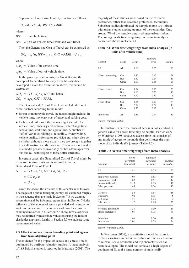
72

Suppose we have a simple utility function as follows:

1 2 3iU a IVT a OVT a FARE= + +

where:

IVT = In-vehicle time.

OVT = Out-of-vehicle time (walk and wait time).

Then the Generalised Cost of Travel can be expressed as:

1 3 2 3 3/ / /i iGC a a IVT a a OVT FARE U a= + + =

where:

a1/a

3= Value of in-vehicle time

a2/a

3= Value of out-of-vehicle time.

In the passenger rail industry in Great Britain, theconcept of Generalised Journey Time has also beendeveloped. Given the formulation above, this would bewritten as:

GJTi

= IVT + a2 / a

1 OVT and hence:

GCi

= a1/a

3 GJT

i + FARE.

The Generalised Cost of Travel can include different‘time’ factors according to the mode:

� for car or motorcycle travel, the factors might include: In-vehicle time, monetary cost of travel and parking cost;

� for bus and rail travel, the factors might include: In-vehicle time, monetary cost of travel, interchange time,access time, wait time, and egress time. A number of‘softer’ variables relating to reliability, overcrowding,vehicle quality, information provision etc. might also beincluded, although more usually they are brought togetherin an alternative specific constant. This is often referred toas a modal penalty as invariably car has advantages overbus and rail with respect to these softer attributes.

In certain cases, the Generalised Cost of Travel might beexpressed in time units and is referred to as theGeneralised Time of Travel:

GTI

= IVT + a2 / a

1 OVT + a

3 / a

1 FARE

= GCi a

3 / a

1

= Ui / a

i

Given the above, the structure of this chapter is as follows.The stages of a public transport journey are examined roughlyin the sequence they are made In Section 7.3 we examineaccess time and, by inference, egress time. In Section 7.4, theinfluence of the amount of service provided and its impact onwait time is examined. The influence of in-vehicle time isexamined in Section 7.5. Section 7.6 shows how elasticitiesmay be inferred from attribute valuations using the ratio ofelasticities approach. Lastly, in Section 7.7,we indicate somerecommended values.

7.3 Effect of access time to boarding point and egresstime from alighting point

The evidence for the impact of access and egress time isdominated by attribute valuation studies. A meta-analysisof 183 British studies is reported in Wardman (2001). The

majority of these studies were based on use of statedpreference, rather than revealed preference, techniques.Suburban studies dominated the sample (some two-thirds)with urban studies making up most of the remainder. Onlyaround 7% of the sample comprised inter-urban studies.The average walk time weightings in the meta-analysisdataset are shown in Table 7.1.

Table 7.1 Walk time weightings from meta-analysis (inunits of in-vehicle time)

StandardContext Mode Mean error Sample

All All 1.68 0.05 183

Urban commuting Car 1.37 0.12 29Bus 1.67 0.14 10Other 1.99 0.16 29

Urban leisure Car 1.74 0.15 25Bus 1.66 0.23 13Other 1.97 0.35 9

Urban other Car 1.55 0.10 34Bus 2.02 0.22 13Other 1.37 0.17 8

Inter urban All 1.51 0.14 13

Source: Wardman (2001)

Table 7.2 Access time weightings from meta-analysis

Value Standard(in-vehicle deviation Number

Category time mins) of value of studies

All 1.81 0.75 52

Employers business 1.95 0.65 10Commuting (peak) 1.62 0.54 12Leisure (off-peak) 2.13 0.93 17Other purposes 1.43 0.54 13

Car users 1.54 0.54 16Bus users 1.98 0.15 5Rail users 1.31 0.43 4Other users 2 0.88 27

Revealed preference 1.38 0.59 11Stated preference 1.91 0.75 41

Suburban 1.46 0.56 18Inter-urban 2.01 0.78 34


In situations where the mode of access is not specified, ageneral value for access time may be helpful. Earlier workby Wardman (1998) analysed access time that consists ofany mode of access to the mode that constitutes the mainmode of an individual’s journey (Table 7.2).

In Wardman (2001), a quantitative model that aims toexplain variations in individual values of time as a functionof relevant socio-economic and trip characteristics hasbeen developed. The model has achieved a high degree ofgoodness of fit, and a large number of statistically

73

significant, correct sign and plausible variations in thevalues of time have been estimated. Compared to otherfindings with relatively simple tabulations, the modelprovided a significant advance. It should be noted that thismodel is estimated using the dataset in the abovementioned meta-analysis.

Based on the estimated model, the author providesillustrative figures for a range of circumstances for themoney value of in vehicle time and weighting of walktime, wait time and headway. The walk time weighting isreported in Table 7.3, while other values are reported inthe following sections of the chapter. It should be notedthat Table 7.1 reports the average value in the database,while Table 7.3 reports the value implied by the model,which is estimated using the same database.

preference analysis. The attribute weights held by users ofdifferent modes are shown in Table 7.4.

Table 7.4 Walk values in association with interchangeattributes, Edinburgh

95%Value (IVT confidence

Attribute Users mins / trip) interval

Walk time at interchange Bus 1.6 27%Walk time to bus Car 1.3 40%Between stations walk time Rail 3.7 32%

Source: Wardman et al. (2001b)

Table 7.5 Service elasticities, with range and standarddeviation according to average values – Bus

No ofStandard measure-

Run Elasticity Range deviation ments

Short run 0.38 0.10 to 0.74 0.135 27Long run 0.66 0.22 to 1.04 0.275 23

Sources: Appendix to Chapter 7

Table 7.6 Service elasticity, with range and standarddeviation according to average values - Rail

No ofStandard measure-

Run Elasticity Range deviation ments

Run not stated* -0.49 -0.33 to -0.65 0.23 2Short run 0.75 0.65 to 0.90 0.13 3

* Based on headway.

Sources: Appendix to Chapter 7.

Table 7.3 Walk time weightings implied by thequantitative model (in units of in-vehicle time)

Time Distance Under-(mins) (miles) Car Bus Rail ground

2 2 2.18 1.68 1.28 1.55 2.79 2.15 1.65 1.9310 3.37 2.59 1.99 2.3320 4.07 3.13 2.4 2.82

2 10 1.72 1.49 1.14 1.335 2.2 1.91 1.46 1.7110 2.66 2.3 1.77 2.0820 3.21 2.78 2.13 2.5

2 25 1.5 1.39 1.07 1.255 1.92 1.79 1.37 1.610 2.32 2.16 1.65 1.9420 2.8 2.6 1.99 2.34

2 50 1.35 1.32 1.02 1.185 1.74 1.7 1.3 1.5210 2.09 2.05 1.57 1.8420 2.53 2.47 1.9 2.23

2 100 1.22 1.26 0.97 1.135 1.57 1.61 1.24 1.4510 1.89 1.95 1.49 1.7520 2.28 2.35 1.8 2.12

2 200 1.1 1.2 0.92 1.075 1.41 1.53 1.18 1.3810 1.71 1.85 1.42 1.6620 2.06 2.23 1.71 2.01


In the table, the first two columns refers to the assumedwalk time and distance travelled. The next four columnsreport the walk time weighting by each user type indifferent mode (e.g. how bus users value walk time for busmode). The most noticeable feature of the IVT values ofwalk is that they vary considerably. In part this is becauseof differences in the money value of IVT by user type andmode, but there are other strong influences at work. Theincrease in the IVT values of walk time as the levels ofwalk time increase is quite clear, as is the fall in the valuesas distance increases.

Wardman et al. (2001b) provide a valuation of walktime in relation to interchange facilities, based on stated

7.4 Effect of service intervals

The effect of service intervals can be measured in anumber of ways: total vehicle kilometres or hours,frequency, headway/service interval, wait time andschedule delay. Evidence is a mixture of elasticity andattribute value measures.

7.4.1 Elasticity based evidenceThe dominant indicator is vehicle kilometres. Table 7.5indicates that bus demand is relatively insensitive toservice change with a short-run elasticity of approximately0.4 and a long run elasticity of 0.7.

Table 7.6 shows that urban rail may be more sensitivethan bus to service change but the evidence is limited to asmall number of short-run estimates.

The importance of service quality to meeting the needs ofpublic transport customers and decreasing reliance on thecar is indicated by the findings of Arsenio’s (2000)examination of railway demand in Spanish cities (Table 7.7)

74

The author states that

The main results that have to be pointed out are thevalues of elasticities with respect to rail quality andprice. In both cases railway demand appears to beinelastic, although it shows a greater response withrespect to quality changes than to prices.

Arsenio estimates a short-run service elasticity of 0.53and long-run of 0.83 (with quality defined as number ofplaces-km offered by operator RENFE divided by lengthof suburban rail network at each city). For large cities, aservice elasticity of 0.78 is reported and, for small cities,0.39. Arsenio explains these findings and points to theimportance of service quality to maintaining publictransport’s market share particularly in large cities saying:

While in large cities the standard result of a higher (inabsolute terms) demand elasticity with respect toquality than to prices is found, in smaller cities the twovalues are much closer, although their difference isstatistically significant. This implies that commutersin larger cities implicitly value quality improvementsmore than their counterparts in smaller urban areas.Such different valuation could be due to the trafficconditions faced by car users in each case. Highercongestion rates over longer distances for car driversin large cities can explain a higher willingness tochange mode in response to improvements in railwayquality taking the form of increased frequencies and/or available space.

Dargay and Hanly (1999) note that there is a strongpositive correlation between vehicle kilometres operatedper capita and journeys per capita. They have illustratedthe results with a scattergram (Figure 7.1).

Increasing vehicle kilometres operated increasesridership, according to Dargay and Hanly (1999), but theelasticities vary greatly from study to study. However, theelasticity of off-peak travel was greater than for the peak.Service elasticity is lower in Metropolitan areas than inrural areas (Dargay and Hanly (1999). This is likely to bebecause the rural service is poorer and thereforeimprovements on that service will have a greater impact ondemand. The two regions with the lowest level of service,the English Shire counties and Wales also have the lowestlevels of patronage. It is further noted that Scotland showsthe highest level of service and the middle level ofpatronage while London had the highest level of patronagebut the second highest level of service, and EnglishMetropolitan areas had the second highest level ofpatronage and the middle level of service. Overall, Dargayand Hanly recommend short run service elasticities of 0.4,rising to 0.8 in the long run (see also Table 7.5 whichrecommends values of 0.38 and 0.66 respectively).

Service elasticities were also estimated by time of dayby Preston (1998). The main finding was that demand inthe evening and on Sunday was sensitive to service butdemand in the inter-peak period was insensitive to service.

Table 7.7 Elasticities for Spanish cities

Elasticity Large cities Small cities

Price -0.30 -0.32Service quantity (Train kms) 0.78 0.39

Table 7.8 Service elasticities - Bus (Metropolitan PTE)

Description Elasticity

Short runEarly morning/peak 0.38Inter-peak 0.17Evening 0.35Saturday 0.52Sunday 1.05

Long runEarly morning/peak 0.58Inter-peak 0.30Evening 1.95Saturday 0.67Sunday 1.61

All periods 0.13

Source: Preston (1998)

0

20

40

60

80

100

120

140

160

180

200

0 10 20 30 40 50 60 70 80 90

Bus kms per capita

Jou

rney

s pe

r ca

pita

Tyne & Wear

London

W Midland

NorthumbriaDevon

Avon

BuckinghamshireW Sussex

Durham

Figure 7.1 Relationship between bus vehicle kilometres and bus journeys in English counties (average 1987 to 1996)(Dargay and Hanly, 1999)

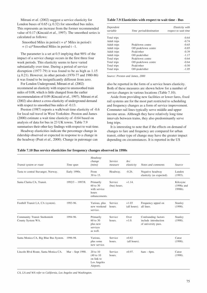
75

Mitrani et al. (2002) suggest a service elasticity forLondon buses of 0.65 (+ 0.32) for smoothed bus miles.This represents an increase from the former recommendedvalue of 0.17 (Kincaid et al., 1997). The smoothed series iscalculated as follows:

Smoothed Miles in period t = a* Miles in period t+ (1-a)*Smoothed Miles in period t –1.

The parameter is a set at 0.5 implying that 90% of theimpact of a service change occurs in the first three fourweek periods. This elasticity seems to have variedsubstantially over time. During a period of servicedisruption (1977-79) it was found to be as high as 1.15(+ 0.21). However, in other periods (1970-77 and 1980-86)it was found to be insignificantly different from zero.

For London Underground, Mitrani et al. (2002)recommend an elasticity with respect to unsmoothed trainmiles of 0.08, which is little changed from the earlierrecommendation of 0.09 (Kincaid et al., 1997). Mitrani et al.(2002) also detect a cross-elasticity of underground demandwith respect to smoothed bus miles of -0.13.

Preston (1987) reports a walk/wait time elasticity of -0.6for local rail travel in West Yorkshire. Preston and James(2000) estimate a wait time elasticity of -0.64 based onanalysis of data for bus in 23 UK towns. Table 7.9summarises their other key findings with respect to wait time.

Headway elasticities indicate the percentage change inridership observed or expected in response to a change inthe headway (Pratt et al., 2000). Change in patronage can

also be reported in the form of a service hours elasticity.Both of these measures are shown below for a number ofservice changes in various locations (Table 7.10).

Aside from providing new facilities or lower fares, fixedrail systems are for the most part restricted to schedulingand frequency changes as a form of service improvement.Commuter rail lines typically serve middle and upperincome areas. Although they have relatively long timeintervals between trains, they also predominantly servelong trips.

It is interesting to note that if the effects on demand ofchanges to fare and frequency are compared for urbantransit, either type of change may have the greater impactdepending on circumstances. It is reported in the US

Table 7.9 Elasticities with respect to wait time - Bus

Dependent Elasticity withvariable Time period/destination respect to wait time

Total trips -0.64Adult trips -0.74Adult trips Peak/town centre -0.65Adult trips Off-peak/town centre -0.85Adult trips Peak/other -0.39Adult trips Off-peak/other -1.17Total trips Peak/town centre -0.64Total trips Off-peak/town centre -0.64Total trips Peak/other -0.50Total trips Off-peak/other -1.05

Source: Preston and James, 2000

Table 7.10 Bus service elasticities for frequency changes observed in 1990s

Headwaychange Service Arc

Transit system or route Time span (mins) measure elasticity Notes and comments Source

Tasta to central Stavanger, Norway. Early 1990s. From Headway. -0.26. Negative headway Lunden30 to 15. elasticity (as expected). (1993).

Santa Clarita CA, Transit. 1992/3 – 1997/8. Primarily Service +1.14. Kilcoyne60 to 30 (bus) hours. (1998a andwith service 1998b).hoursenhancements.

Foothill Transit LA, CA (system). 1993-96. Various, plus Service +1.03 Frequency upped on Stanleynew weekend hours. (all hours). all lines. (1998).service.

Community Transit Snohomish 1994-96. Primarily Service Over Confounding factors StanleyCounty System WA. 60 to 30 hours. +1.0. include introduction (1998).

plus new of university pass.servicesas well.

Santa Monica CA, Big Blue Bus System. 1996-98. Various, Service +0.82 Catoeplus some hours. (all hours). (1998).new service.

Lincoln Blvd Route, Santa Monica CA. Mar – Sept 1990. 20 to 10 Service +0.97. 6am – 6pm. Catoe(40 to 10 hours. (1998).on link toLos AngelesAirport).

CA, LA and WA refer to California, Los Angeles and Washington.

76

Transportation Research Board Interim Handbook (Pratt etal., 2000) that in Dallas, the following fare and serviceelasticities were calculated in the period 1985-87 whenfare and service changes were introduced (Table 7.11).

The Isotope Research Study (European Commission,1997) reported service elasticities for bus in a number ofEuropean cities by city size (small: population<500,000)(see Table 7.13).

Table 7.13 Service elasticities for bus in European cities

Elasticity Small city Large city

Service 0.33 0.49

Table 7.11 Fare and service elasticities - Dallas

Fare elasticity Service elasticity

Urban bus -0.35 +0.32Suburban express bus -0.26 +0.38Suburban local -0.25 +0.36

Table 7.12 Service elasticities - New Zealand

Source Public transport kilometres elasticity

Christchurch 1975-89 0.4 to 0.5Auckland 0.6726 NZ Urban areas 1.0Wanganui 1978-85 0.7Wellington Rail 1970-85 0 to 0.5International ‘standard’ values 0 to 0.8Average elasticity 0.51Standard deviation 0.34

Source: Adapted from Wallis and Yates (1990)

The authors describe these findings as:

…statistical analysis covering two years of fare andservice changes in greater Dallas revealed greatersensitivity to fares than service in the center city, andthe converse in the suburbs, for both suburban expressand local services. (Allen, 1991).

The effect of route and schedule restructuring ondemand for travel in Riverside, California has beendescribed in the handbook:

The restructuring was accomplished in the Fall of1995 within the constraint that total bus service hoursnot be increased by more than 4 percent. Ridershipincreased by 20.4 percent over the prior year. Routerestructuring focused on enhancing direct travel. Theschedule restructuring emphasized consistency andease of transfer, in addition to providing increasedfrequency on heavily travelled routes within the servicehours constraint. All schedules were standardized tobe on 15, 30 or 60 minute on-the-hour headways(Stanley, 1998)

The handbook suggests that the effects of waiting timeare influenced by a number of external factors. Forinstance, protection from weather in wet, hot or coldclimates makes a difference in a rider’s perception ofwaiting and transfer times.

Outstanding responses to service hours and frequencyenhancements in Santa Clarita and Santa Monica,California (elasticities of +1.14 and +0.82 respectively)were accompanied by aggressive marketing ranging fromdirect mail campaigns and free-ride coupons to imagebuilding keyed to a striking new bus paint design (Stanley,1998; Catoe, 1998).

Wallis and Yates (1990) have estimated serviceelasticities for New Zealand as shown in Table 7.12.

Demand is shown to be more service elastic in big citiesthan small ‘because of the competition from other publictransport modes’ (European Commission, 1997). Thereport also suggests that service is valued more highly inlarge cities due to higher income levels with the impliedvalues of service being 0.54 ECUs per bus km in smallcities and 1.44 ECUs in large cities.

Service frequency also has a strong impact on publictransport demand elasticity. Elasticity for low frequencyservices is greater than for high frequency services.Cheung (citied in Booz Allen Hamilton, 2003) foundelasticities for lower frequency services were up to fourtimes greater than high frequency services.

Scheduling and frequency modifications are among themost common service changes that transit operators maketo improve service effectiveness. According to Pratt et al.(2000), scheduling and frequency most particularly affectthat aspect of transit service quality which is the waitingtime patrons encounter and perceive in making a transittrip. Individual changes may have the objective ofreducing wait time at the start of a transit trip, orminimizing wait time if a transfer between two vehicles isrequired. Scheduling changes may be made to increase theease of passenger comprehension of the schedule. Relatedactions may have the objectives of improving thereliability of the service, reducing both real and perceivedpassenger wait times, and lowering passenger anxiety.These service quality objectives support the goals ofproviding a more attractive service, increasing transitridership, and shifting travel out of low occupancy autos.

FitzRoy and Smith (1998a) studied the demand for railtransportation in European countries and described thesignificance of high frequencies for maintaining market share:

With respect to passenger rail, Switzerland, theNetherlands and Eire were most successful inmaintaining their share of the market during the1980s. This may be partly explained by the fact thatthe former two countries, in particular, are notable fortheir extremely high train frequencies.

Ford and Haydock (1992) identify two mainphilosophies of timetable planning for the passengermarket. The first consists of trying to provide passengercarrying capacity exactly when and where detailed marketresearch shows it is needed, maximising seat occupation asfar as possible. This approach is described as market-led(or perhaps more accurately demand-led). The authorsdescribe SNCF as market-led saying:

SNCF is the leading exponent of tailoring the timetableexactly to the travel market. Many of its trains havevariations on Friday, Saturday, Sunday and Monday,with only Tuesday to Thursday having the same service.

77

The second approach involves providing a ‘regular intervaltimetable’ which maximises frequency and regularity. This isdescribed as being production-led, but a case could be madefor this approach being described as market–led. ‘Clockface’departures are easily remembered by passengers and staff butmay force passengers to adapt to train times which may notsuit them. Ford and Haydock go on to describe theintroduction of production-led timetabling:

Once traffic on a line reaches a level where more than10-15 trains, spread throughout the day, are justified,the timetable planner may decide to operate the servicewith a regular stopping pattern at a regular hourlyinterval; this is known as a clock-face or regularinterval timetable (RIT).

RITs have been common throughout Europe for manyyears, particularly on intensive suburban services, but lessso on Inter City routes. The successful Verbund regionallycoordinated services described by Pucher and Kurth(1995) in Hamburg, Munich, Rhein-Ruhr, Vienna andZurich provide a service at

…regular intervals to make schedule easier for ridersto remember and to facilitate transfers between linesand different public transport modes.

When Austrian Federal Railways (ÖBB) inaugurated theirNAT 91 (Neue Anstro-Takt) network of seven principalroutes operated at two-hourly frequencies, train kilometreswere increased by over a quarter and by over 41% for fastesttrains (Schnellzuge). Earlier introductions of regular intervaltimetables in Switzerland had produced patronage increaseof up to 30% on specific areas, although the introduction ofa nationwide system (Taktfrahrplan) in 1982 did notproduce large patronage increases but did prevent trafficlosses. Similarly, introduction of regular interval timetablein Belgium in 1984 led to small increases in demand (up2%) and receipts (up 8%) in the following year (Ford andHaydock, 1992).

7.4.2 Attribute value based evidenceWardman (2001) provides a meta-analysis of 62 studies inwhich wait time was a service attribute. The results areshown in Table 7.14. It was found that wait time wasvalued at about 1.6 times in-vehicle time for urban bus and1.2 for underground rail.

The results of assessing 56 such studies are given inWardman (1998) and are shown in Table 7.15. Thesefindings indicate the impact of schedule delay is valued at0.34 in-vehicle time minutes for bus and 0.9 for rail. Theseare less than the wait time values, particularly for bus.

Table 7.14 Wait time weightings from meta-analysis (inunits of in-vehicle time)

StandardContext Mode Mean error Sample

All All 1.76 0.10 62

Urban Bus 1.59 0.22 11UG 1.17 0.04 11Car and PT 2.06 0.14 30

Inter All 1.70 0.28 10


Table 7.15 Departure time shift weightings frommeta-analysis



All 0.72 0.64 56Employers business 0.57 0.31 12Commuting (peak) 1.03 1.08 14Leisure (off-peak) 0.58 0.52 12Other purposes 0.69 0.32 18Car users 0.61 0.72 31Bus users 0.34 0.19 2Rail users 0.9 0.51 23Urban 0.44 0.23 6Suburban 1.06 1.26 9Inter-urban 0.82 0.41 20General 0.58 0.48 21Depart earlier 0.64 0.59 23Depart later 0.69 0.71 24Depart either earlier or later 1.03 0.58 9


Table 7.16 Wait time weightings implied by thequantitative model (in units of in-vehicle time)

Time Distance Under-(mins) (miles) Car Bus Rail ground

2 2 3.68 2.57 2.51 2.935 4.25 2.97 2.9 3.3810 4.73 3.31 3.24 3.7720 5.28 3.69 3.61 4.2

2 10 2.9 2.29 2.24 2.65 3.35 2.64 2.58 3.0110 3.73 2.94 2.88 3.3520 4.16 3.28 3.21 3.74

2 25 2.53 2.14 2.09 2.415 2.92 2.47 2.42 2.8110 3.26 2.75 2.69 3.1320 3.63 3.07 3 3.5

2 50 2.28 2.03 1.99 2.315 2.64 2.35 2.3 2.6710 2.94 2.62 2.56 2.9820 3.28 2.92 2.85 3.32

2 100 2.06 1.93 1.89 2.25 2.38 2.23 2.18 2.5410 2.65 2.49 2.43 2.8320 2.96 2.77 2.71 3.16

2 200 1.86 1.84 1.8 2.095 2.15 2.12 2.07 2.4210 2.39 2.36 2.31 2.6920 2.67 2.64 2.58 3

As in Section 7.3, Wardman (2001) provides illustratingexamples of wait time weighting for a range ofcircumstance based on the estimated quantitative model.The results are reported in Table 7.16.

In other studies the weight placed on departure time shiftsrelative to travellers’ desired departure times are considered.

78

Similar to the in-vehicle-time (IVT) value of the walktime, the IVT value of wait time varies considerably. Asthe level of wait time increases or the distance traveldecreases, the IVT value of wait time increases.Comparing Table 7.16 to Table 7.3, for correspondinglevels of walk and wait time and the same journeydistance, the values of wait time tend to be greater than thevalue of walk time.

Another way of considering service interval attributes isin terms of the headway. Wardman (2001) provides ananalysis of 164 British studies in which headwayweightings were specified (Table 7.17). The key findingwas that headway weightings were slightly less than unityat around 0.77.

� there is a pronounced effect on interchange penalty fromdistance;

� commuters have lower values than leisure travellers;

� car users have very much higher values than publictransport users.

In geographical terms, Wardman reports that values ofinterchange penalty for travellers in the south east are lower,despite their higher income on average, saying this is:

…presumably a function of the familiarity and highservice frequency effect, whilst it may also be thatinterchange facilities are better in the south east andthat there is an appreciation of a more integratedtransport system which uses interchange to promote awider range of journey possibilities within a relativelyhigh quality and large network.

7.5 Effect of changes in time spent on board the vehicle

7.5.1 Elasticity based evidenceNew evidence on elasticities with respect to in-vehicletime is limited but the Victoria Transport Policy Institutesuggests in-vehicle time elasticities of -0.58 for urban bus,-0.86 for urban rail, -2.11 for interurban bus and -1.58 forinterurban rail (based on Small and Winston, 1999).

Gunn et al. (1998) have estimated the total door-to-door time elasticities of the number of journeys bypurpose for public transport in Paris. The most in-vehicletime sensitive trips are non home-based other (-0.86), theleast in-vehicle time sensitive trips are non home-basedwork (-0.37) (Table 7.20).

Table 7.18 Headway weightings implied by thequantitative model (in units of in-vehicle time)

Under-Distance Purpose Car Bus Rail ground

2 EB 0.88 0.85 0.96 1.122 Non EB 0.71 0.69 0.78 0.9110 EB 0.57 0.62 0.70 0.8110 Non EB 0.46 0.50 0.57 0.6625 EB 0.44 0.52 0.58 0.6825 Non EB 0.36 0.42 0.47 0.5550 EB 0.37 0.45 0.51 0.5950 Non EB 0.30 0.37 0.41 0.48100 EB 0.30 0.39 0.44 0.52100 Non EB 0.25 0.32 0.36 0.42200 EB 0.25 0.34 0.39 0.45200 Non EB 0.20 0.28 0.31 0.37

EB = Business trips

Table 7.19 Value per trip for interchange attributes -Edinburgh

95%Value(IVT confidence

Attribute Users mins / trip) interval

Wait time at interchange (mins) Bus 1.2 22%Guaranteed connection Bus 3.6 42%Interchange wait time (mins) Rail 1.7 39%


Table 7.17 Headway weightings from meta-analysis (inunits of in-vehicle time)

Context Mode Mean Std error Sample

All All 0.77 0.04 164

Urban commuting Car 0.85 0.11 18Bus 0.84 0.20 6Other 0.70 0.17 5

Urban leisure Car 1.00 0.13 19Bus 0.97 0.17 12Other 0.84 0.12 10

Urban EB All 1.22 0.25 5

Urban other Car 0.63 0.07 22Bus 0.61 0.08 13Other 0.75 0.03 4

Interurban commuting All 0.47 0.09 7

Interurban leisure All 0.52 0.07 17

Interurban EB All 0.69 0.11 14

Interurban other All 0.95 0.17 12

Interurban Car 0.63 0.14 7Rail 0.49 0.08 16Other 0.78 0.09 27

The quantitative model developed by Wardman (2001)enables a more detailed breakdown of headway weightingby distance. Table 7.18 provides the implied headwayweighting across distance and purpose which are thefactors which influence it. The strong distance effect isvery apparent, with the headway valuation being muchhigher for shorter distance trips.

In terms of waiting attributes at interchange facilities,Wardman et al. (2001b) report the results of statedpreference analysis of bus and (separately) rail users(Table 7.19). The key finding is that value per trip forinterchange facilities is relatively low ranging from 0.1 to1.7 IVT mins/trip.

Wardman (2001) has also summarised other findings oninterchange, reporting that:

� the interchange penalty is found to increase over time asGDP increases;

79

York (1996) found that bus priority schemes alone have alimited impact on bus patronage. This was believed to be dueto the fact that most priority schemes result in only small timesavings which are not perceived by bus passengers. This wasconfirmed by Daugherty et al. (1999) who reviewed anumber of bus priority schemes in Great Britain. In only oneinstance (Aberdeen), did they find evidence of increasedpatronage. In any event, this patronage growth was modest(4%) and largely attributable to park and ride. Survey worksuggested patronage growth of 1.4% attributable to buspriority (with a range of 0.4% to 4.5%). The observed journeytime reduction on this route was around 3.5% (although theperceived reduction was 9%). This would suggest an in-vehicle time elasticity of around -0.4.

Mackett and Nash (1991) and Mackett and Bird (1989)report in-vehicle time elasticities of between -0.63 and -0.7for rail in general. Steer Davies Gleave (1999a) found theUK average in-vehicle time elasticity for rail to liebetween -0.6 and -0.8.

In-vehicle time elasticities for rail in the south-east ofEngland provided in Mackett and Nash (1991) and Mackettand Bird (1989) are summarised in Tables 7.21 and 7.22.

Preston (1987) has estimated a journey time elasticity of-0.418 for journeys on local rail in West Yorkshire.

Generalised Cost (GC) brings together fare, in-vehicletime, walk time and wait time. GC elasticities vary byjourney purpose. Halcrow Fox et al. (1993) reportedGeneralised Cost elasticities for bus in the range of -0.4 to-1.7, for underground of -0.4 to -1.85 and for British Railof between -0.6 and -2.00 (Table 7.23).

The rail industry in Great Britain makes use of theconcept of Generalised Journey Time which consists ofstation to station journey time, a service interval penaltyand an interchange penalty. The Passenger DemandForecasting Handbook (Association of Train OperatingCompanies, 2002) recommends a default GeneralisedJourney Time elasticity for rail journey of less than 30miles of –0.9. For journey above 30 miles, this value variesdepending on the attractiveness of rail (measured by Qwhich is Generalised Journey Time divided by distance)and the strength of competition from other modes.

7.5.2 Attribute value based evidenceThe value of in-vehicle time, the ratio of the importance oftime spent on board to fare paid, provides a means to derivejourney time elasticities from fare elasticities. The value ofin-vehicle time also enables attributes expressed in units ofin-vehicle time to be converted into money values.

The TRACE project found that most car driver valuesof time are generally higher than those of public transportusers. This difference is partly attributed to a ‘selection’effect: a person for whom time is of high value tends tochoose fast modes. It could also be an income effect:

Table 7.20 Total journey time elasticities of number ofjourneys by public transport bypurpose - Paris

Purpose of trip Public transport time elasticity

Work – white collar -0.51Work – blue collar -0.55Business -0.24Education -0.74University -0.41Regular shop -0.74Other shop -0.6Other -0.56Non home-based work -0.37Non home-based other -0.86

Table 7.21 In-vehicle time elasticities – Rail

Run Short Medium Long

Average in-vehicle time elasticity -0.74 -0.51 -0.84Standard deviation 0.3727 0.212 0.41No of observations 6 2 6

Based on models of the Chiltern Line and South-East Sector

Table 7.22 In-vehicle time elasticities – All modes

Description Elasticity

All modes trips to central London, -0.98Chiltern line corridor, short run

All modes trips to central London, -0.26South-east sector corridor, short run

All modes trips to central London, -1.13Chiltern line corridor, long run

All modes trips to central London, -0.34South-east sector corridor, long run

Source: Mackett and Nash (1991) and Mackett and Bird (1989)

Table 7.23 Generalised cost elasticities

Purpose Mode Low income Medium income High income

Home - work Bus -0.40 to -0.50 -0.50 to -0.70 -0.60 to -0.80Underground -0.40 to -0.60 -0.50 to -0.70 -0.70 to -0.90BR -0.60 to -0.70 -0.70 to -0.90 -0.80 to -1/0

Home - other Bus -1.30 to -1.50 -1.40 to -1.60 -1.50 to -1.70Underground -1.40 to -1.60 -1.50 to -1.70 -1.65 to -1.85BR -1.30 to -1.50 -1.60 to -1.70 -1.70 to -2.00

Employers business Bus -0.60 to -0.80Underground -0.50 to -0.70BR -1.50 to -2.00

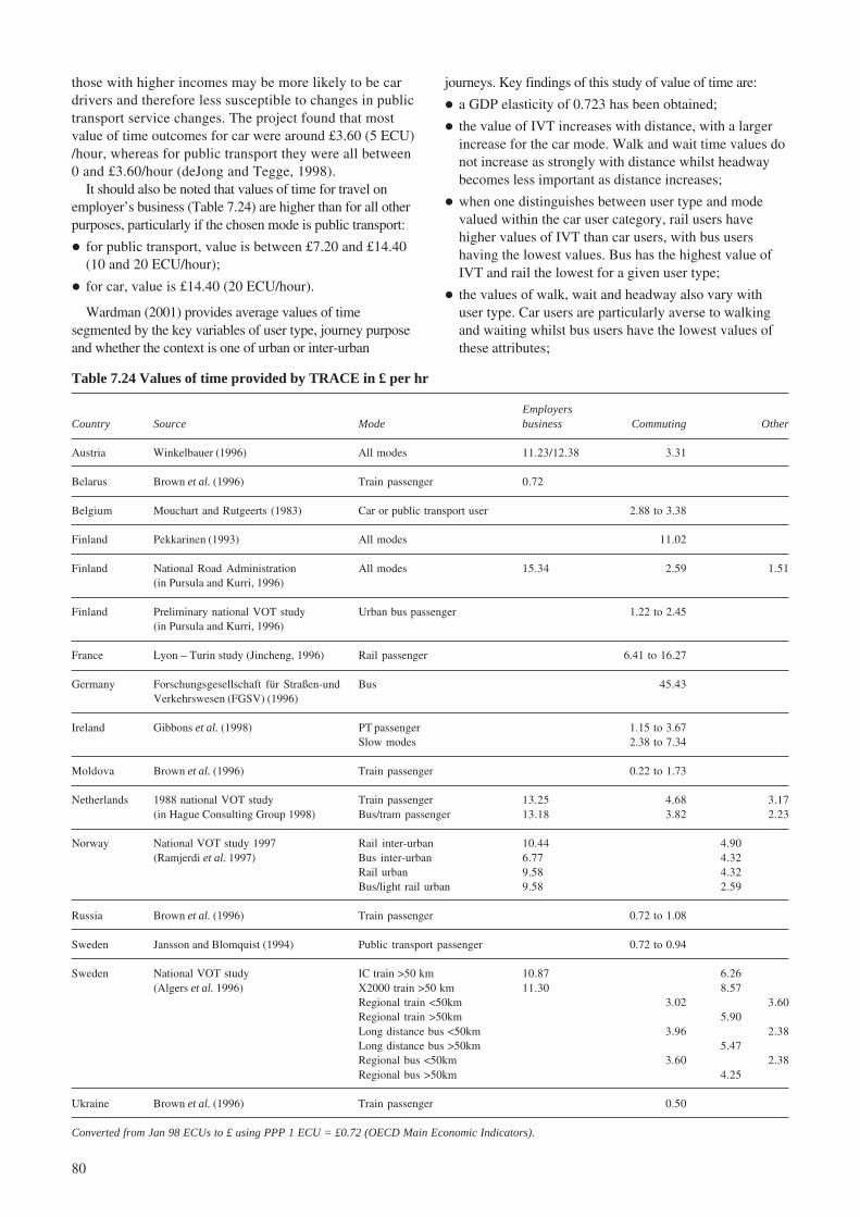
80

those with higher incomes may be more likely to be cardrivers and therefore less susceptible to changes in publictransport service changes. The project found that mostvalue of time outcomes for car were around £3.60 (5 ECU)/hour, whereas for public transport they were all between0 and £3.60/hour (deJong and Tegge, 1998).

It should also be noted that values of time for travel onemployer’s business (Table 7.24) are higher than for all otherpurposes, particularly if the chosen mode is public transport:

� for public transport, value is between £7.20 and £14.40(10 and 20 ECU/hour);

� for car, value is £14.40 (20 ECU/hour).

Wardman (2001) provides average values of timesegmented by the key variables of user type, journey purposeand whether the context is one of urban or inter-urban

journeys. Key findings of this study of value of time are:

� a GDP elasticity of 0.723 has been obtained;

� the value of IVT increases with distance, with a largerincrease for the car mode. Walk and wait time values donot increase as strongly with distance whilst headwaybecomes less important as distance increases;

� when one distinguishes between user type and modevalued within the car user category, rail users havehigher values of IVT than car users, with bus usershaving the lowest values. Bus has the highest value ofIVT and rail the lowest for a given user type;

� the values of walk, wait and headway also vary withuser type. Car users are particularly averse to walkingand waiting whilst bus users have the lowest values ofthese attributes;

Table 7.24 Values of time provided by TRACE in £ per hr

EmployersCountry Source Mode business Commuting Other

Austria Winkelbauer (1996) All modes 11.23/12.38 3.31

Belarus Brown et al. (1996) Train passenger 0.72

Belgium Mouchart and Rutgeerts (1983) Car or public transport user 2.88 to 3.38

Finland Pekkarinen (1993) All modes 11.02

Finland National Road Administration All modes 15.34 2.59 1.51(in Pursula and Kurri, 1996)

Finland Preliminary national VOT study Urban bus passenger 1.22 to 2.45(in Pursula and Kurri, 1996)

France Lyon – Turin study (Jincheng, 1996) Rail passenger 6.41 to 16.27

Germany Forschungsgesellschaft für Straßen-und Bus 45.43Verkehrswesen (FGSV) (1996)

Ireland Gibbons et al. (1998) PT passenger 1.15 to 3.67Slow modes 2.38 to 7.34

Moldova Brown et al. (1996) Train passenger 0.22 to 1.73

Netherlands 1988 national VOT study Train passenger 13.25 4.68 3.17(in Hague Consulting Group 1998) Bus/tram passenger 13.18 3.82 2.23

Norway National VOT study 1997 Rail inter-urban 10.44 4.90(Ramjerdi et al. 1997) Bus inter-urban 6.77 4.32

Rail urban 9.58 4.32Bus/light rail urban 9.58 2.59

Russia Brown et al. (1996) Train passenger 0.72 to 1.08

Sweden Jansson and Blomquist (1994) Public transport passenger 0.72 to 0.94

Sweden National VOT study IC train >50 km 10.87 6.26(Algers et al. 1996) X2000 train >50 km 11.30 8.57

Regional train <50km 3.02 3.60Regional train >50km 5.90Long distance bus <50km 3.96 2.38Long distance bus >50km 5.47Regional bus <50km 3.60 2.38Regional bus >50km 4.25

Ukraine Brown et al. (1996) Train passenger 0.50

Converted from Jan 98 ECUs to £ using PPP 1 ECU = £0.72 (OECD Main Economic Indicators).

81

� the values of walk and wait time vary with the levelsthey take. The variation seems plausible. For walk timethe variations in the values seems to centre around twicein-vehicle time but they are higher for wait time.

The values of IVT are reported in Table 7.25 and areexpressed in year 2000 quarter 3 prices. Two sets offigures are given according to the elasticity used to accountfor income growth. One adjustment uses an elasticity ofone as used by the then Department of the Environment,Transport and the Regions in its recommended procedures.The other adjustment involves an income elasticity of 0.5,in line with cross-sectional evidence from the first Britishvalue of time study (MVA et al., 1987), the second British

Table 7.26 Department of the Environment, Transportand the Regions – Values of Time

Business – driver 39.7Business – rail 57.3Business – Underground 48.1Non work 8.5

Table 7.25 Overall values of IVT (pence per minute,quarter 3, 2000 prices)

Income Incomeelasticity = 1 elasticity = 0.5

Context Std. Std.Mode Mean error Mean error Sample

Urban commuteCar 6.0 0.4 5.5 0.4 64Bus 4.2 1.0 3.8 0.8 17Rail 7.2 0.9 6.2 0.7 17Underground 9.2 0.9 8.2 0.8 5Car and PT 7.6 0.7 5.8 0.4 44

Urban leisureCar 6.5 0.5 5.8 0.4 73Bus 2.6 0.3 2.4 0.3 22Rail 6.5 1.0 5.7 0.8 14Underground 7.3 0.7 6.5 0.6 16Car and PT 4.7 0.5 4.3 0.4 25

Urban businessCar 13.2 3.6 11.7 3.1 11Rail and Underground 19.2 9.0 17.8 8.3 8

Urban otherCar 6.4 0.4 5.8 0.4 84Bus 3.2 0.3 2.9 0.3 27Other 6.4 0.8 5.5 0.6 29

InterurbanCar 10.5 1.8 10.0 1.7 11Rail 12.6 0.8 11.5 0.8 21Other 9.1 1.0 7.7 0.9 9

Interurban leisureCar 9.2 1.1 8.2 1.0 23Rail 13.3 1.2 12.0 1.1 44Car and PT 13.7 1.5 11.8 1.4 10Other 11.7 1.3 10.0 1.1 8

Interurban businessCar 18.3 2.6 17.6 2.6 16Rail 32.2 3.5 29.3 3.3 34Rail 1st 52.3 5.7 46.0 5.4 17Car and PT 13.7 1.5 11.8 1.4 11

Interurban otherCar 7.4 0.5 7.4 0.6 10Rail 17.6 1.5 15.3 1.3 18Other 8.6 0.9 7.6 0.8 15


value of time study (Hague Consulting Group and AccentMarketing and Research, 1999), studies in the Netherlands(Gunn, 2001) and previous time series evidence frommeta-analysis (Wardman, 2001).

A number of relationships are apparent within the figurespresented in Table 7.25. Inter-urban trips have generallysomewhat higher values than urban trips and, as expected,employer’s business trips have higher values than trips forother purposes. For urban trips, commuting journeys havehigher values than leisure trips for all modes other than car.For inter-urban trips, there is little difference between thevalues of time for commuting and leisure.

The values of time vary quite appreciably according tothe mode used. For urban journeys, underground (UG)users appear to have the highest values whilst bus usershave the lowest values. The figures seem to indicate thatrail users have higher values than car users, particularly forinter-urban trips although there may be a distance effect atwork here since inter-urban rail trips tend to be longer thaninter-urban car trips.

The Department of the Environment, Transport and theRegions (2001d) recommended values of time for a numberof categories contained in Table 7.26. These are behaviouralvalues and hence directly comparable with those containedin Table 7.25. They have been adjusted from mid 1998prices and income to 2000 quarter 3 prices and incomeusing the recommended income elasticity of one.

Wardman says that as far as non-work travel isconcerned, the recommended values seem to be far toohigh for urban trips yet too low for inter-urban trips.Across all trips, however, the recommended non-workvalue compares favourably with the large amount ofempirical evidence.

Table 7.25 reports the average value of time in the meta-analysis dataset; a more detailed breakdown of value oftime by user types, modes and distances, as implied by thequantitative model estimated using the same dataset, ispresented in Table 7.27. Absolute values in pence perminute and 2000 quarter 3 prices are given as well as ratiosof these values to car users’ values of car IVT.

Car users’ values of car are higher than for train andgenerally lower than for bus. Although car time doesbecome more highly valued than bus time, this only occursat long distances where there are very few observations forbus travel. We are unable to test whether there is anypositive incremental effect on the distance elasticity forbus journeys over long distances.

The distance and journey purpose effects are readilyapparent as are the low values of bus users and the highvalues of rail users. The figures are in stark contrast torecommended values in that they exhibit a considerableamount of variation.

82

7.6 Inferring elasticities from attribute valuations

There is plenty of evidence on most of the main effects. Inaddition, evidence can be inferred from knowledge ofprice elasticities and valuations of attributes through theratio of elasticities approach. There is limited evidence onbreak-downs by city type, time of day/week, journeypurpose, socio-economic group but what evidence there issuggests that these segmentations are important.

In this section, some illustrative examples are given,where the ratio of elasticities approach is used to deriveelasticities with respect to certain attributes. It should benoted that the values derived should be viewed asindicative rather than definitive. This is because it is verydifficult to obtain the real value of the input factors, suchas fare elasticities, value of the attributes, mean level of theattributes, etc. As a result, the derived elasticity will beaffected by the accuracy of the input values. Nevertheless,the examples not only provide indications of the elasticityvalues with respect to certain attributes and their variationacross segments, but also illustrate the relationshipbetween different attribute values and elasticities.

Table 7.28 illustrates the elasticities for bus demandwith respect to in-vehicle-time varies for various journeytypes. In this example, the mean level of IVT, fareelasticity and average fares are UK national average figureand they are constant across segments. As a result, theparameter in the formula that determines the IVT elasticityis the value of IVT. As there is marked difference of IVTvalues for the business trips and other trips, the IVTelasticity is also substantially higher for the business trips.

For each journey purpose, the IVT elasticity is lower forrail demand than that for bus demand (Table 7.29). This ismainly due to the effects of higher average fares for rail

Table 7.29 Elasticities for rail demand with respect toIn-Vehicle-Time (IVT) by journey purpose

Value Meanof IVT level Average

Journey Elasticity (pence/ of IVT Fare farestype wrt IVT minute)a (minutes)b elasticityc (pence)d

Commute -0.42 9.00 31.00 -0.51 336.41Leisure -0.27 5.10 31.00 -0.58 336.41Business -0.53 13.50 31.00 -0.43 336.41

Source: a. Table 7.27; b. Average journey length 31 miles from DETR1999; mean speed is assumed to be 60 mph; c. Table 6.34;d. Calculated from total passenger receipt and total passenger journeyfrom DETR (1999).

Table 7.28 Elasticities for bus demand with respect toIn-Vehicle-Time (IVT) by journey purpose




Source: a. Table 7.33; b. Average journey length 4 miles from DETR 1999;mean speed is assumed to be 12 mph; c. Table 6.4; d. Calculated from totalpassenger receipt and total passenger journey from DETR (1999).

journeys. Although the travel time costs for rail travel are alsohigher than bus, the relative value of total IVT compared tofares is lower for rail. Consequently, the sensitivity of raildemand to IVT change is lower than the bus mode, althoughthe sensitivity of rail demand to fare change is higher.

Table 7.27 Money values of IVT implied by the quantitative model

Absolute values Relative to car users’ values of car time

Under-User type Miles Bus ground Rail Car Car Car Bus

Under- Under-Mode valued Bus ground Rail Rail Bus Car Bus ground Rail Rail Bus

Comm 2 3.0 9.5 5.7 4.4 6.1 4.6 0.65 2.05 1.23 0.95 1.3310 4.0 12.7 7.6 5.9 8.2 7.0 0.58 1.82 1.09 0.84 1.1825 4.8 15.1 9.0 7.0 9.8 8.9 0.54 1.70 1.01 0.79 1.1050 7.0 n/a 13.2 10.3 14.3 13.8 0.51 n/a 0.96 0.75 1.04100 n/a n/a 15.0 11.7 n/a 16.5 n/a n/a 0.91 0.71 n/a

Leis 2 2.7 5.1 5.1 4.0 5.5 4.2 0.65 1.22 1.23 0.95 1.3310 3.7 6.8 6.9 5.3 7.5 6.3 0.58 1.08 1.09 0.84 1.1825 4.3 8.1 8.1 6.3 8.8 8.0 0.54 1.01 1.01 0.79 1.1050 6.4 n/a 12.0 9.3 13.0 12.4 0.51 n/a 0.96 0.75 1.04100 7.2 n/a 13.6 10.5 14.7 14.9 0.48 n/a 0.91 0.71 0.99200 8.2 n/a 15.5 12.0 16.7 17.8 0.46 n/a 0.87 0.67 0.94

EB 2 7.1 13.4 13.5 10.4 14.6 11.0 0.65 1.22 1.23 0.95 1.3310 9.6 18.0 18.1 14.0 19.6 16.7 0.58 1.08 1.09 0.84 1.1825 11.4 21.3 21.4 16.6 23.2 21.2 0.54 1.01 1.01 0.79 1.1050 16.7 n/a 31.5 24.4 34.2 32.8 0.51 n/a 0.96 0.75 1.04100 19.0 n/a 35.8 27.8 38.8 39.2 0.48 n/a 0.91 0.71 0.99200 21.6 n/a 40.7 31.5 44.1 46.9 0.46 n/a 0.87 0.67 0.94

Comm = Commuting trips.

Leis = Leisure trips.

EB = Business trips.

83

Tables 7.30 and 7.31 show that the ratio of elasticityapproach is not only useful in deriving IVT elasticity, butis applicable to other attributes, such as wait time and walktime. The wait time elasticity for bus demand is lower thanthe IVT elasticity. This is because that the total wait timecosts is lower than the total journey time costs, so thesensitivity of bus demand to wait time change isconsequently lower. The walk time elasticities show asimilar picture except that the business travel hasmarginally higher walk time elasticity than IVT elasticity.However, it should always be borne in mind that theexamples given here are illustrative as the real values ofthe parameters are very difficult to establish.

With respect to service levels, we find from Table 7.32 ashort run elasticity of bus demand with respect to vehiclekms of 0.38, rising to 0.66 in the long run, although wewould expect this to vary by time of day, by the existinglevel of service and by other factors. Evidence on local rail’sservice elasticity is more sparse but Table 7.32 suggests thatit might be higher than that of local bus. This might reflectthat improved local rail services almost always abstractdemand from local bus services whereas improved local busservices only rarely abstract demand from local rail. Wefind, based on 62 observations, that wait time is valued at1.76 times the value of IVT. However, for short bus trips,where wait time forms a large element of generalised cost,we would expect wait time values to be in excess of twicethose of IVT. We find, based on 164 observations, that onaverage headway is valued at 0.77 times the value of IVT.As expected this is less than half the value of wait time,reflecting that time spent waiting at a bus stop is valuedmore highly (i.e. has greater disutility) than time spentwaiting at home, work or elsewhere.

Table 7.30 Elasticities for bus demand wrt Wait-Time(WTT) by journey purpose




Source: a. Table 7.27 and 7.14; b. By assumption; c. Table 6.4;d. Calculated from total passenger receipt and total passenger journeyfrom DETR (1999).

Table 7.31 Elasticities for bus demand wrt Walk-Time(WKT) by journey purpose




Source: a. Table 7.27 and 7.1; b. By assumption; c. Table 6.4;d. Calculated from total passenger receipt and total passenger journeyfrom DETR (1999).

7.7 Conclusions

This chapter has examined a mix of elasticity measuresand attribute values for three factors: access/egress, serviceintervals and in-vehicle time. The summary of theempirical evidence on these three factors is as follows.

In terms of access/egress, we find walk time is valuedon average at 1.68 times the value of IVT, based on 183observations. However, values vary with the overall triplength and the amount of walk time. For short bus tripswith considerable amounts of walking to and from the busstop values in excess of 2.0 may be found. Whenconsidering all possible access modes (including park andride, kiss and ride and feeder bus) access time is found tobe valued on average at 1.81 time the value of IVT (basedon 52 observations). This higher valuation may in partreflect an interchange penalty.

Table 7.32 Service elasticities, with range and standarddeviation according to average values - busand rail

Standard No. ofElasticity Range deviation measurements

Bus short run 0.38 0.10 to 0.74 0.14 27Rail short run 0.75 0.65 to 0.90 0.13 3Bus long run 0.66 0.22 to 1.04 0.28 23

With respect to in-vehicle time, evidence on elasticities islimited, particularly for bus. This may reflect that bus speedsare often beyond the control of operators, being largelydetermined by traffic conditions. Our best estimates are thata representative in-vehicle time elasticity for local bus mightbe in the range of -0.4 to -0.6, whilst for rail this might be-0.6 to -0.8. There is substantially more evidence onpassenger valuations. At 2000 prices, we find the meanvalue of time for commuting by urban bus as 4.2 p/min(based on 17 observations), whilst for leisure travel by urbanbus it is 2.6p/min (based on 22 observations). For urban rail,we find the corresponding values to be 7.2 p/min forcommuting (based on 17 observations) and 6.5 p/min forleisure (based on 13 observations)

8 Effects of quality of service: other factors

8.1 Introduction

This chapter discusses a number of service quality factorswhich are not directly measurable in terms of time,although there may be time elements in some cases. Forexample, the effect of an interchange on demand maydepend on both the time taken to effect the transferbetween services and the quality of the interchange areaand the facilities provided. Other factors considered arewaiting environment, service reliability, vehicle qualityand a number of bus-specific issues.

In addition to elasticity information, the relativeimportance of quality of service characteristics is often

84

expressed in terms of an attribute weighting relative toanother journey component. This weighting may be in termsof equivalent in-vehicle time. For example, a real timeinformation system may equate to a 3 minute reduction ofin-vehicle time per trip. Alternatively, service attributes maybe expressed in money terms, such as a minute of wait timebeing worth the equivalent of 10 pence in fare.

This chapter includes literature on attribute weightingsbecause, when incorporated within demand forecastingprocedures, they provide a crucial input in determiningpassenger responses to enhanced service levels.

Various types of forecasting procedure can be used. Inbrief, the possible techniques include:

� Converting attribute weightings into an equivalent farechange. When combined with an appropriate priceelasticity the equivalent fare change can be used toestimate demand changes.

� Equivalent generalised cost change. This has someparallels with the fare method and requires a generalisedcost elasticity, the journey time and cost componentsthat make up generalised cost, and the correspondingweightings for each of these components.

� Ratio of elasticities. With a knowledge of an elasticityfor one user group, market shares for different groupsand journey characteristics, the elasticities for other usergroups may be determined (see Section 5.6).

Studies that include attribute weightings are usuallycommissioned by local authorities or transport operatorsand carried out by consultancies. Such studies rarely enterthe public domain. Meta analysis of such studies, however,avoids the need to report individual studies and hencemaintains anonymity.

A typical forecasting framework based on attributeweightings is that adopted in the PDFH which convertseach attribute change into an equivalent change in rail fareand takes the form:

[( ({F newI F C RS OB SF= − + + +}* ) / )] f

base baseIP SY CS F F+ + +where:

IF

is the proportionate change in demand.

Fnew

and Fbase

are the fares in the new and forecast yearsrespectively.

C is the value of Crowding changes (= baseaverage crowding cost minus new averagecost of crowding, expressed as a % of basicfare divided by 100).

RS is the value of Rolling Stock changes (% ofbase fare divided by 100).

OB is the value of On Board Facilities changes(% of base fare divided by 100).

SF is the value of Station Facilities changes (%of base fare divided by 100).

IP is the value of Information Provisionchanges (% of base fare divided by 100).

SY is the value of Security changes (% of basefare divided by 100).

CS is the value of Cleanliness changes (% ofbase fare divided by 100).

f is the fare elasticity for the market segment.

Note that if Fnew = Fbase, then the index of demand is:

( ){ }f

FI I C RS OB SF IP SY CS= + + + + + +

Reporting weightings in terms of the equivalent in-vehicle time avoids the need to adjust money values fromthe estimation year to the year in which application is takingplace. Thus, when a study reports both time and moneyequivalents only the time equivalent is reproduced here.

The European Local Transport Information Service(ELTIS) describes quality factors that it feels a publictransport service needs to exhibit in order to be a desirablealternative to a car:

� travel time door-to-door must be competitive;

� comfort must be noticeably improved;

� comfort and feeling of safety in relation to connectionsbetween modes at interchange points are important; and

� provision of information to the traveller at home (onroutes, timetables etc) and individual marketing are apart of promoting a modern public transport system thatis not restricted to its role of providing a social servicefor those without a car.

In addition, ELTIS suggests that services for transportusers must try to address the problems which prevent theuse of public transport. These obstacles include:

� logistical barriers: lack of ticket integration,uncoordinated timetables;

� financial barriers: cost differential between public andprivate transport;

� psychological barriers: poor perception of travel timeand image, lack of control over journey, poor perceptionof true cost of car travel;

� institutional barriers: impact of competition betweenoperators, impact of deregulation;

� information barriers: lack of appropriate information,lack of co-ordinated information;

� physical barriers: accessibility, comfort, travel timedifferential; and

� social barriers: personal safety and security.

Improvements in service quality can help to overcomethese barriers, for example, increased publicity about thetrue cost of private and public transport will lead to a betterinformed public, while ensuring that up-to-dateinformation on services is readily available can helppeople make better choices of public transport.

8.2 Effect of the waiting environment

In describing the main features of the successful regionalVerbund services, Pucher and Kurth (1995) say:

…bus stops and stations have been expanded,modernized and redesigned to improve the comfortand safety of passengers waiting to transfer from onebus line to another, or between rail and bus lines.

85

Above all, passengers are now better protected fromthe weather, and pedestrian access has been improved,both for the transfer from one public transport modeor line to another, and from the surroundingneighborhood.

Steer Davies Gleave (1996) estimated values for busstop characteristics by means of stated preference analysis.Table 8.1 summarises these findings.

of originating and interchanging passengers. For short-distance passengers, a minimum value of 36p per journey,in 2000 prices, should be applied. These values will behigher for more extensive station improvements, especiallythose which affect longer distance inter-urban andinterchanging passengers. A typical package of extensiveimprovements might include a travel centre, waitingrooms, provision of monitors/shelter, ticket office, tannoysystem and toilets. Any such package should have amaximum value of 10% of the fare and care should betaken to ensure that enhancements such as the provision ofpassenger information are not double counted.

The PDFH notes that station improvements will exhibitdiminishing returns when considered as a package. Thusreducing valuations by 70% to 80% of their individualvaluations in well designed studies and 40% to 50% instudies prone to biases. However, there may be increasingreturns when the station facilities on a whole line arerefurbished. There are also certain aspects of station designthat can be assessed in terms of journey time. Anyrefurbishment that affects the queues at ticket offices or thedelays at ticket barrier etc. can be measured in terms oftime savings. Any such time savings should be valued atleast twice as highly as in-vehicle time. In addition theprovision of facilities at interchange stations will alsoreduce the interchange penalty at these stations. Table 8.3provides some values for a range of station improvementsfor interchanging passengers, which can also be applied tooriginating passengers.

Table 8.1 Value per trip for bus stop facilities - London

Attribute Value (1996 pence / trip)

Shelter with roof and end panel 5.6Basic shelter with roof 4.5Lighting at bus stop 3.1Moulded seats at bus stop 3.4Flip seats at bus stop 2.2Bench seats at bus stop 0.9Dirty bus stop -11.8

Source: Steer Davies Gleave (1996) in Bristow and Shires (2001)

Table 8.2 Value per trip for interchange facilities,Edinburgh

95%Value confidence

Attribute (IVT mins/ trip) interval

Shelters/bus stopsShelter with lighting, roof and end panels and seats 1.7 ±13%Shelter with lighting and roof 1.2 ±16%A newsagents 0.3 ±63%

Shelters/station interchangeClosed circuit television 0.8 ±20%Intercom connection to control room 0.5 ±32%Eating and drinking facilities 0.4 ±47%Toilets 0.7 ±21%

Station interchangeStaff presence 1.1 ±24%Good signs showing where buses go from 1.2 ±22%Change machine 0.1 ±117%

Sources: Wardman et al. (2001b)

Table 8.3 Interchange station facilities

Commute Business Leisure

Intercom to control centre 4 23 20Real time information monitors 23 38 37Additional Staff Present 10 15 30CCTV 10 14 13Heated and refurbished waiting room 5 7 10Clear departure information 3 21 21Plenty of seats on platform 17 25 24Better lighting 3 4 4Additional printed timetable information 0 12 12

Values are in pence per journey at 2000 quarter 4 prices and incomes.Adjustments for inflation and income growth should be made in the samemanner as outlined for the value of time and for overcrowding values.

Source: ATOC (2002).

Steer Davies Gleave (1996) recommends that a packageof service enhancements, including those in other tables inthis chapter, be capped at 26.1 pence, on the basis of statedpreference analysis of a package of enhancements.

Wardman et al. (2001b) provide a range of evidence ofdifferent bus stop and terminal facilities (see Table 8.2).

Hensher and Prioni (2002) find that seats and shelter at abus stop are valued at around 7 pence per trip, whilst a seatalone is valued at around 3 pence.

For rail, MVA (2000b) report an average value for astation refurbishment of 19.4p per one-way journey in1990 prices, or 11% of the average fare. This was based ona stated preference survey of 100 users of refurbishedstations in Lancashire. This suggests that values for railmay be higher than for bus.

The typical value for a station refurbishment package isquoted in the PDFH as being worth up to 5% of the fares

8.3 Staff and security

The PDFH notes that the availability, the quality and theattitude of front-line staff towards customers, has asignificant effect on passengers’ perceptions of rail travel.Good and helpful staff can minimise the effects of anotherwise poor service. Alternatively, poor staff attitudecan damage the perceptions of all aspects of a train service.

Another area where the presence of staff has an importantinfluence is the perception of security and safety bypassengers. A number of potential passengers, particularlywomen and the elderly are deterred form using rail atparticular times because of fears about personal security.

Evidence from surveys suggests that staffing and visibility

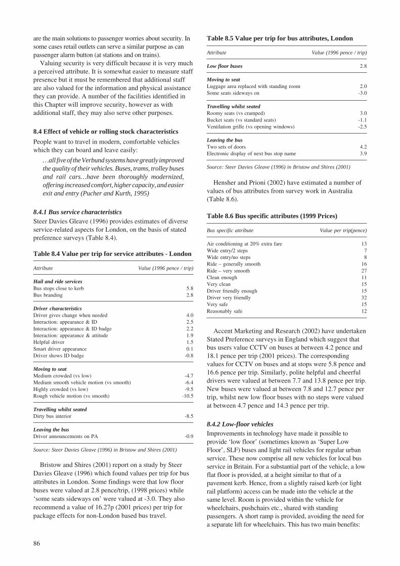
86

are the main solutions to passenger worries about security. Insome cases retail outlets can serve a similar purpose as canpassenger alarm button (at stations and on trains).

Valuing security is very difficult because it is very mucha perceived attribute. It is somewhat easier to measure staffpresence but it must be remembered that additional staffare also valued for the information and physical assistancethey can provide. A number of the facilities identified inthis Chapter will improve security, however as withadditional staff, they may also serve other purposes.

8.4 Effect of vehicle or rolling stock characteristics

People want to travel in modern, comfortable vehicleswhich they can board and leave easily:

…all five of the Verbund systems have greatly improvedthe quality of their vehicles. Buses, trams, trolley busesand rail cars…have been thoroughly modernized,offering increased comfort, higher capacity, and easierexit and entry (Pucher and Kurth, 1995)

8.4.1 Bus service characteristicsSteer Davies Gleave (1996) provides estimates of diverseservice-related aspects for London, on the basis of statedpreference surveys (Table 8.4).

Hensher and Prioni (2002) have estimated a number ofvalues of bus attributes from survey work in Australia(Table 8.6).

Table 8.5 Value per trip for bus attributes, London


Low floor buses 2.8

Moving to seatLuggage area replaced with standing room 2.0Some seats sideways on -3.0

Travelling whilst seatedRoomy seats (vs cramped) 3.0Bucket seats (vs standard seats) -1.1Ventilation grille (vs opening windows) -2.5

Leaving the busTwo sets of doors 4.2Electronic display of next bus stop name 3.9


Table 8.6 Bus specific attributes (1999 Prices)

Bus specific attribute Value per trip(pence)

Air conditioning at 20% extra fare 13Wide entry/2 steps 7Wide entry/no steps 8Ride – generally smooth 16Ride – very smooth 27Clean enough 11Very clean 15Driver friendly enough 15Driver very friendly 32Very safe 15Reasonably safe 12

Table 8.4 Value per trip for service attributes - London


Hail and ride servicesBus stops close to kerb 5.8Bus branding 2.8

Driver characteristicsDriver gives change when needed 4.0Interaction: appearance & ID 2.5Interaction: appearance & ID badge 2.2Interaction: appearance & attitude 1.9Helpful driver 1.5Smart driver appearance 0.1Driver shows ID badge -0.8

Moving to seatMedium crowded (vs low) -4.7Medium smooth vehicle motion (vs smooth) -6.4Highly crowded (vs low) -9.5Rough vehicle motion (vs smooth) -10.5

Travelling whilst seatedDirty bus interior -8.5

Leaving the busDriver announcements on PA -0.9


Bristow and Shires (2001) report on a study by SteerDavies Gleave (1996) which found values per trip for busattributes in London. Some findings were that low floorbuses were valued at 2.8 pence/trip, (1998 prices) while‘some seats sideways on’ were valued at -3.0. They alsorecommend a value of 16.27p (2001 prices) per trip forpackage effects for non-London based bus travel.

Accent Marketing and Research (2002) have undertakenStated Preference surveys in England which suggest thatbus users value CCTV on buses at between 4.2 pence and18.1 pence per trip (2001 prices). The correspondingvalues for CCTV on buses and at stops were 5.8 pence and16.6 pence per trip. Similarly, polite helpful and cheerfuldrivers were valued at between 7.7 and 13.8 pence per trip.New buses were valued at between 7.8 and 12.7 pence pertrip, whilst new low floor buses with no steps were valuedat between 4.7 pence and 14.3 pence per trip.

8.4.2 Low-floor vehiclesImprovements in technology have made it possible toprovide ‘low floor’ (sometimes known as ‘Super LowFloor’, SLF) buses and light rail vehicles for regular urbanservice. These now comprise all new vehicles for local busservice in Britain. For a substantial part of the vehicle, a lowflat floor is provided, at a height similar to that of apavement kerb. Hence, from a slightly raised kerb (or lightrail platform) access can be made into the vehicle at thesame level. Room is provided within the vehicle forwheelchairs, pushchairs etc., shared with standingpassengers. A short ramp is provided, avoiding the need fora separate lift for wheelchairs. This has two main benefits:

87

� Certain types of passenger not previously able easily tomake use of bus and light rail services can now do so.These include wheelchair users, and those with shoppingtrolleys and/or child pushchairs. Some other categories,notably the elderly may also find access easier

� Dwell time at stops is reduced, especially in comparisonwith older light rail vehicles in which several steps haveto be negotiated by passengers. Topp (1999) estimatessavings of up to 40%, giving reductions in journey timeanalogous to those through priority measures and off-vehicle ticketing. However, for buses the reduction inboarding and alighting times tends to be off-set by theadditional time needed for vehicles to kneel and rise.The net effect on dwell times depends on numbers ofboarders and alighters at each stop. York and Balcombe(1998) found that on a typical London route, the overalltime for a single-deck low-floor vehicle exceeded thatfor a conventional double-deck vehicle byapproximately one minute.

As in other cases of innovation, low-floor access mayoften by combined with other service quality measures,such as improved driver training and better passengerinformation, Extensive publicity given to introduction oflow-floor buses and new colour schemes may themselvesattract new users, simply through increased awareness.Some very high percentage growth figures must thus betreated with caution. York and Balcombe (1998) studiedthe effects of introducing low-floor buses on five Londonbus routes and one in North Tyneside. Changes inpatronage ranged from -6.7 to +17.0%, but in most casesthere were comparable changes on nearby control routes Itwas possible to identify a significant change due to low-floor buses on only one London route: the apparentincrease was 11.8%. Some examples showing the range ofgrowth encountered in other areas, excluding extremeinstances, but not necessarily taking overall demand trendsinto account, are given below:

Kentish Bus 480 (Gravesend - Dartford) 5% (LocalTransport Today, 1996).

Blackpool 22% - associated with extensive publicity(Transit, 1997).

Ipswich 2-3% (Coach & Bus Week,1997).

Plymouth 5% (Transit, 1998a).

Birmingham (Travel West Midlands) route 9 5%(Transit, 1998b).

Birmingham (Claribels) 9% (Coach & Bus Week, 2000b).

Truronian, Cornwall (rural service) 15% (DETR, 1998b).

London route 242, operated by Arriva 10% (Coach &Bus Week, 1999).

Southampton - Winchester (Solent Blue Line) 7.5%(Coach & Bus Week, 2000a).

Southampton cross-city route 5% and Southampton-Eastleigh 3.5% (Solent Blue Line) (Transit, 2000).

While cases of substantial simultaneous changes inservice and fare levels have been excluded, it may be thecase that some of the larger growth figures are associatedwith simultaneous marketing initiatives, etc. as well asintroduction of low-floor vehicles.

York and Balcombe (1998) assessed the effects of low-floor buses on the travel habits of ambulant disabledpassengers and passengers with pushchairs. The resultsshowed that ambulant disabled passengers in Londonvalued low-floor buses at one penny per trip more than atrip in a double-decker and that in Tyneside the differencewas 57 pence more per trip. The reason for the largedifferential was attributed to the free travel available topassengers in London that resulted in considerableresistance to any form of payment. The values reported bythose people with pushchairs (both areas) was between 4pand 12p per trip in favour of low floor buses, giving anaverage value of around 7.4p per trip compared with a tripon a double-decker.

8.4.3 New railway rolling stockWardman and Whelan (2001) provide a comprehensiveassessment of the impact of new railway rolling stock inGreat Britain. A novel feature was the development ofrevealed preference (RP) models based on actual choicesbetween different stock types to complement traditionalstated preference (SP) models. A total of 2348 RP and7047 SP choices were available. The joint RP-SP choicemodel contained journey time, egress time, headway,crowding levels, fare and the ratings of different rollingstock types. The cost coefficient was allowed to vary withincome whilst the time and stock coefficients varied withjourney purpose. The values obtained expressed asproportions of the fare or journey time are given below. Incontrast to the vast majority of other evidence, the valuesare on the low side (Table 8.7).

The study also used SP methods to estimate the separatevalues associated with ride quality, seating layout, seatingcomfort, noise, ventilation and ambience. This was doneby reference to the levels existing on different types oftrain with which the respondent would be familiar. As in anumber of other studies, a package effect was present inthat the sum of the values of individual attributes exceededthe estimated value of the overall package.

Table 8.7 Railway rolling stock valuations

Stock types (preferred first) Money value Time value Moneyvalue Timevalue

Express sprinter v sprinter 0.9% 1.9% Mark 2 v SE slam door 1.4% 2.2% Networker v sprinter 0.7% 0.8% Mark 3 v SE sliding door 1.5% 2.0% Express sprinter v SE slam door 1.5% 3.0% Mark 2 v SE sliding door 0.7% 1.0% SE sliding door v SE slam door 0.6% 0.9% Mark 3 v networker 0.6% 1.1% Networker v SE slam door 1.0% 1.1% Mark 2 v networker 0.6% 1.3% Wessex electric v SE slam door 1.2% 2.8% Mark 3 v Mark 2 0.1% 0.2%

88

It was found that refurbishment which changes the levelof seating layout, ride quality, ventilation, ambience, noiseand seating comfort from levels associated with old southeast slam door stock to new air conditioned south eaststock was worth around 2.5% of the fare. However, mostrefurbishments would be worth somewhat less than this,with 1.5% being a representative figure.

The report also reviewed evidence relating to thepackage effect across four studies as well as providingfresh evidence. The average package effect across thesestudies was 0.5, indicating that the sum of the valuations ofindividual stock attributes is, on average, twice the valueof the corresponding overall package.

In addition, a large-scale review of 18 previous SPstudies was conducted. The values tended to be high. Itwas suspected that many had been subject to strategicresponse bias. These high valuations were not supportedby eight studies based on analysis of ticket sales as in fourstudies there was no significant change in demand afternew rolling stock introduction whilst in the other fourdemand increases of between 3% and 8% were found butwith broad confidence intervals.

A regression model was developed to explain thevariations across 45 valuations of rolling stock expressedas a proportion of the fare paid. A variable denotingwhether the purpose of the study would have been readilyperceived to have been stock valuation found that rollingstock values were three times higher in such instances.This was taken to signify the presence of strategicallybiased responses. In addition, familiarity with the types ofnew rolling stock being proposed was found to yieldvalues 44% lower than where there was unfamiliarity. Theresults of this review do allow some degree ofreconciliation between the findings of econometricanalysis of ticket sales data and the values obtained fromstated preference studies.

8.4.4 CrowdingThere has also been considerable work on valuing theimpact of overcrowding in the passenger rail industry. Arecent study is that of MVA (2000a). This study wasundertaken for the Strategic Rail Authority and itsobjective was to value the benefits from alleviatingcrowding on services to and from London. A statedpreference survey was used which featured cost, journeytime and different crowding conditions in which thejourney was made. The services surveyed were GNER andMidland Mainline services to and from London, outersuburban services of South West Trains and Chiltern andInner Suburban services of South West Trains and LTS.Surveying was conducted in February 2000 and a sampleof over 2000 passengers was obtained.

Models were estimated for inner suburban, outersuburban, intercity leisure, intercity commute, intercitybusiness and intercity first class. Within each set of flows,models were estimated for a number of other categories,such as journey purpose, journey time, income group,gender and age group. The results for the main categoriesof interest are given below. The values are expressed inpence per minute in quarter 1 2000 prices and incomes.

The results are not entirely consistent. For example, theresults for InterCity 1st class are not plausible whilst thereare several other cases where the relationship betweenvaluations does not conform to expectations.

Table 8.8 Values of time in different crowdingconditions (p/min)

Flow S1 S2 S3 S4 S5

Inner suburban commute 7.7 11.4 10.4 24.1 28.0Outer suburban commute 18.6 11.6 15.3 32.2 31.3Intercity leisure 12.9 8.3 14.0 n.a 37.9Intercity business 123.5 112.6 89.9 n.a 319.3Intercity 1st class -93.9 -92.9 -217.7 n.a n.a

S1 Sitting at the lowest level of crowding.S2 Sitting at the medium level of crowding.S3 Sitting at the highest level of crowding.S4 Standing at the medium level of crowding.S5 Standing at the highest level of crowding.

An alternative approach to evaluation of crowding is touse crowding values in conjunction with fares or generalisedcosts. Crowding values are related to the amount of timespent in a train and are therefore presented as pence perminute values (see Table 8.9). In addition the values vary byjourney and route purpose. With the exception ofcommuting, crowding penalties occur when load factorsreach 60%. The penalties for commuters do not start untilload factors reach 90% and 100%, and are justified becausecrowding is the norm in this market. It should be noted thatthe crowding penalties in Table 8.9 only refer to individualpassengers on particular trains. If values are being calculatedfor average train loads the PDFH recommends that thecrowding penalties are increased by 10%.

8.4.5 On-board facilitiesIt is recognised that on-train catering does affect raildemand, but the PDFH is unable to provide anyrecommended values for catering provision. What is notedis that the cost of not providing catering services onservices that have them advertised is likely to be far higherthan any benefit gained from their presence. There is alsoevidence that suggests trolleys are regarded as a nuisanceand have a negative value. This is contradicted by anotherstudy that found that a trolley was preferable to a buffetcar, with a value of about £3.50.

Clearer evidence exists that passengers are prepared topay higher fares for packages of ‘added service benefits’.These are outlined in Table 8.10 and cover a wide range ofservices. It is, however, unlikely that any of these areapplicable to urban rail journeys.

8.4.6 CleanlinessCleanliness is an important attribute for both commutingand off-peak urban journeys. It is ranked above seatingcomfort for the former and second only to punctuality/reliability for the latter.

The values recommended by the PDFH come from theNetwork SouthEast Quality of Service research. Tworecommended values are made for rolling stock, both

89

extremes. For ‘litter on the floor’, a possible value of 2pper passenger minute is recommended, whilst for ‘litter onfloor and seats’ a possible value of 5p per passengerminute is given. Cleanliness accounts for 1-2% of the 5%value attributed to station refurbishment. Again care needsto be taken to avoid double-counting the cleanlinessbenefit if a refurbishment has taken place.

8.5 Effect of interchanges between modes

Pucher and Kurth (1995) describe Munich as:

…perhaps the premier example of rail systemintegration, with long-distance, medium-distance andshort-distance rail systems merging underneath the

long pedestrian mall extending from Karlsplatz toMarienplatz in the city’s centre

Interchange should be made as easy as possible withinformation readily available on connections and waitingtime minimised and made pleasant. As with any publictransport waiting environment, there should be shelter fromthe weather, security and adequate facilities for comfortsuch as toilets, seats and shops. In addition, efficientinterchange between modes such as car or bike and publictransport can be facilitated through the provision ofadequate parking facilities. Pucher and Kurth (1995) haveidentified this aspect of inter-modal coordination as a factorto encouraging more public transport use:

Table 8.9 recommended crowding penalties for passengers (p / min)

CommutingLeisure Business

LondonNon Non Non 1st Class

Load factor London London London London Inner Outer London London

50% Sit 0.0 0.0 0.0 0.0 0.0 0.0 0.0 0.060% Sit 0.0 0.0 0.0 0.0 0.0 0.0 0.0 0.070% Sit 0.2 0.17 2.4 0.7 0.0 0.0 0.0 0.080% Sit 0.4 0.35 4.7 1.3 0.0 0.0 0.0 0.090% Sit 0.8 0.52 9.2 1.9 0.0 0.25 0.4 6.0100% Sit 1.1 0.70 13.7 2.5 0.6 0.50 0.8 12.1110% Sit 1.5 1.20 18.2 3.6 1.2 0.75 1.2 –120% Sit 1.8 1.70 22.7 4.6 1.8 1.00 1.6 –130% Sit 2.2 2.20 27.2 5.7 2.4 1.25 2.0 –140% Sit 2.5 2.70 31.7 6.7 3.0 1.50 2.4 –150% Sit – – – – 3.6 – – –160% Sit – – – – 4.2 – – –100% Stand 22.0 22.0 100.0 48.0 12.0 12.0 6.5 –120% Stand 26.4 26.4 120.0 50.5 13.0 13.0 7.5 –140% Stand 30.8 30.8 140.0 53.0 14.0 14.0 8.5 –160% Stand – – – – 15.0 15.0 9.5 –

All values are in 2000 quarter 4 prices and incomes.

The values should be inflated to current prices using the retail price index.

Adjustments for income growth should be made by adjusting the business values using a GDP per capita elasticity of 1.0 and adjusting the leisurevalues using a GDP elasticity of 0.723.

All crowding costs are zero at 60% load factor. All intermediate values should be calculated by linear interpolation.

The London / non-London split applies to the trains, not necessarily the passenger’s journey.


Table 8.10 Values associated with on-board facilities

Packages Value £s

Standard class package – segregated accommodation (a quieter 1.30 – leisure and self paid business traveller.environment), free tea/coffee and a tabloid newspaper. 0.16 – season ticket holders.

5.00 – employer-paid business travellers(all above in 1996 prices).

First class premier – free refreshments, quality newspaper, on-train 5.30 – business travellers.magazine, novel/magazine on request, free car parking or taxi (up to 16.10 – leisure travellers.three miles) and breakfast/light snack voucher.

As above but not free car parking or taxi (up to three miles). 0.00 – business travellers.

Standard class premier – free tea/coffee/soft drink, quality newspaper, 0.53 – leisure travellers.on-train magazine and a quiet environment. 2.29 – business travellers (employers pay).

A quiet environment. 0.08 – business travellers (employers pay).1.08 – business travellers (paying for themselves)(all above in 1999 prices).

90

All five Verkehrsverbund in this study dramaticallyincreased the number and capacity of park-and-ridefacilities…and most systems have greatly increasedthe number and quality of bike storage facilities attrain stations, including, sheltered bike racks andconvenient lockers.

Wardman (1998) provided evidence on interchangepenalties from meta-analysis of 47 British studies(Table 8.11). The key finding was that passengersdislike interchange with a reported penalty equivalent to21 minutes for bus and 37 minutes for rail, but note thatthis includes additional walking and waiting time aswell as the inconvenience of interchange per se.

In spite of its importance, public transport demandelasticities (or other quantitative estimates) with respect toservice reliability are limited and often only qualitativeestimates of passenger response to reliability have beenmade. Bly (1976b) is an early work that developed atheoretical model for estimating the effects of randomservice cuts on passenger waiting times (cited by Booz,Allen and Hamilton, 2003). This model indicated that, forhigh frequencies, the percentage increase on averagewaiting times is about twice the percentage of bus servicesnot operated; while for low frequencies this factorincreases to three or more (ie. a 10% random service cutwill increase waiting times by around 20% for frequentservices, 30% or more for less frequent services). Furtherthe ‘excess’ waiting time experienced by passengers islikely to be valued at 2-3 times ordinary waiting time,reflecting the anxiety and annoyance caused.

Noland and Polak (2002) note that there are two mainapproaches to modelling reliability. The first they term themean-variance approach and is the method mostcommonly used in public transport studies. Then secondthey refer to as the endogenous scheduling approach.Examples of the latter are rare in public transport.

An example of the mean –variance approach inrelation to wait time and wait time reliability is the workof WS Atkins and Polak (1997), who estimate weightingsin relation to in-vehicle time, suggesting that the standarddeviation of wait time has a similar weight to the meanvalue of wait time, indicating that delays can have asignificant impact on demand (Table 8.13).

WS Atkins and Polak (1997) also give values for bus in-vehicle time and in-vehicle time reliability (Table 8.14).

Table 8.11 Interchange penalty weightings frommeta-analysis



All 31.29 22.94 47Employers business 32.36 13.46 7Commuting (peak) 14.25 5.26 11Leisure (off-peak) 35.13 25.28 12Other purposes 39.17 26.67 17Car users 13.91 5.64 8Bus users 20.83 9.36 6Rail users 36.8 20.07 13Other users 37.79 27.53 20Revealed preference 43.08 32.86 10Stated preference 28.1 18.81 37Suburban 16.22 8.41 21Inter-urban 43.46 23.8 26


Table 8.13 Values of bus wait time reliability relative toaverage in-vehicle time

By journey purposeBy time period

Journey OtherVariable to work Shopping purposes Peak Off-peak

Wait time 2.6 1.3 3.1 2.6 1.7Wait time s.d. 2.5 1.0 1.9* 3.0 1.2Observations 598 616 254 679 870

* Not statistically significant.

Source: WS Atkins and Polak (1997).

Table 8.14 Values of bus in-vehicle time reliabilityrelative to average in-vehicle time

By journey purposeBy time period

Journey OtherVariable to work Shopping purposes Peak Off-peak

Bus in-vehicle time 1.4 0.8 1.3 1.4 0.9In-vehicle time s.d. 2.0 0.8 2.3 1.8 1.2Rho-sq (0) 0.293 0.189 0.278 0.293 0.205Observations 598 616 254 679 870

Source: WS Atkins and Polak (1997).

On the basis of separate stated preference experimentswith bus, rail and car users, Wardman et al. (2001b) provideattribute values for the interchange penalty and interchangeconnection times shown in Table 8.12. The key findings forEdinburgh, which are dominated by frequent, intra-urbanservices, were a value per trip for interchange penalty of 5minutes for bus and 8 minutes for rail.

8.6 Reliability

Qualitative and attitudinal studies of travel choicebehaviour have found that the punctuality, reliability anddependability of a transport system are rated by users as avery important feature, affecting both their perceptions andlevels of use for different modes.

Table 8.12 Value per trip for interchange attributes -Edinburgh

Value 95%User (IVT mins/ confidence

Attribute type trip) interval

Interchange penalty Bus 4.5 ±65%Interchange penalty Car 8.6 ±83%Interchange connection time (mins) Car 1.7 ±61%Interchange penalty Rail 8 ±78%Change platform walk time (mins) Rail 1.5 ±79%


91

Hensher and Prioni (2002) find that bus reliability (in termsof minutes late) is valued at around 1.82 times in-vehicletime. Accent (2002) found that if buses were always on time,this would be valued at between 4.2 and 18.2 pence per trip(2001 prices).

As well as SP work, there are also some cases whereresearchers have calculated an observed elasticity ofdemand with respect to ‘lost km’ compared with scheduledchanges. In London, estimates of the impact of schedulecoverage’ gave an elasticity of about +1.5 to +1.6,compared with an overall elasticity with respect to bus-miles of +0.78 (Kennedy et al., 1995). This ratio is similarto work by Bly reported in the original handbook andreferred to above.

Noland and Polak (2002) discuss the concept of thereliability ratio, defined as the value of travel timevariability (measured by the standard deviation of traveltime) over the value of travel time. They report that for railcommuters this values is between 1.04 and 1.22 but forleisure travellers this ratio was estimated to be around 0.66.

An example of the endogenous scheduling approachapplied to the rail industry is described by Bates et al.(2001). They quote a value of expected schedule delayearly of 56 pence per minute, compared to a value ofschedule delay late of 114 pence per minutes. They alsofind a value of headway of 5 pence per minute and a valueof delay of 127 pence per minute of delay. However, theirsurvey work included business travellers with high valuesof time. The Passenger Demand Forecasting Handbookinterpreted this work as implying, on average, a value oflate time of around 3 times that of in-vehicle time. Most ofthis was due to the annoyance of being late but asignificant element (equivalent to 0.5 times the value of in-vehicle time) was due to penalties associated withrescheduling activities. This was a particularly prominentfeature for commuters using high frequency servicesbecause they have tightly constrained schedules.

8.7 Effect of information provision and promotionalactivity

8.7.1 General effectsGood passenger information is an essential ingredient of asuccessful public transport system; ill informed travellersmay not be able to identify services which best suit theirneeds, leading to poor perceptions and low use of publictransport.

Information provision and promotional activity can takemany forms.A good review is provided by Rickman(1991) using West Yorkshire PTE (Metro) as a case study.Metro’s general policy has been:

‘the promotion of the network in such a way as tomaintain and increase patronage, by good informationabout the services available, prompt notification ofchanges, encouraging loyalty to the public transportsystem, presenting a unified system of services to thepublic and seeking to make non users aware of thesignificant benefits of public transport’ (West YorkshirePTE/Metro, 1991).

To these ends Metro provides a number of publicityservices (in the broadest sense):

Timetable leaflets.These are the main source of detailed information toenable usage of the system. They are distributed via MetroTravel Centres, bus and rail stations, libraries and TouristInformation Centres. Metro will post up to ten timetablesto those requesting them (but the service is not heavilyadvertised). Leaflets are not distributed to householdsdespite trials that illustrate the cost effectiveness of thismethod (Ellson and Tebb, 1978, 1981, found that revenueincreases were three to ten times greater than costs in aninitial five month period) nor are they usually distributedon-vehicle.

Timetables are the main source of publicity for publictransport despite the fact that research has indicated that70% of those making regular journeys and 60% ofoccasional passengers never consult timetables (Balcombeand Vance, 1998). In West Yorkshire, it has been foundthat 42% of those using buses once a month had atimetable leaflet in their home, but only 37% were surethat it was up to date (Harris Research Centre, 1989). Thisindicates that bus travel is largely an experience good.People gain information on the product from theirexperience of using it.

Area guidesBus and train guides for each of West Yorkshire’s fivedistricts are produced annually including route maps andsummaries of the services in the area. The first version ofthese guides was distributed to all households butsubsequently they have been distributed in the samemanner as timetable leaflets.

Metro travel centresCentres in Leeds, Bradford, Huddersfield and Halifax areopen 0830 - 1730 Monday to Friday and 0900 - 1630Saturdays, whilst bus companies also have travelinformation centres. Harris Research Centre (1989) foundthat 35% of bus users had visited a travel centre in theprevious year, with 85% being able to find all theinformation they require.

Telephone enquiry service

Metro has set up a Busline system. A survey by Bonsalland Tweddle (1990) indicated that 96% of callers weresatisfied with the service but that on average demand wasdouble the number of callers getting through to Busline. Itwas estimated that Busline led £450k of extra revenue perannum.

Information at bus stops, bus and rail stations Of the 13,600 bus stops maintained by Metro, timetablecases are provided at 2,650. This coverage of around 20%is significantly better than the other PTEs but it is stillsurprising that 80% of sales outlets for bus travel in WestYorkshire have no information at all about the product

92

they are selling. Moreover, the information displayed isnormally based on the timetable leaflets and is verydifficult to read. Experiments with information based ondeparture times from the stop were undertaken but havesince been abandoned.

West Yorkshire PTE have experimented with computerinformation points at Brighouse, Cleckheaton andNormanton, but have not supplied real time informationwhich advises customers when vehicles will arrive atstops. Evidence on whether such systems increasepatronage is mixed. Work on London Underground(Sheldon et al., 1985, Forsyth and Silcock, 1985) and inOttowa, Canada (Suen and Geehan, 1986) indicate thatdemand can be increased by up to 10%. Evidence fromLondon Buses (Wardman and Sheldon, 1985) and theTyne and Wear Metro (James, 1986) is less positive.

On-board informationMetro’s on-board information is limited to detailsconcerning service changes and advertising materialconcerning pre-paid tickets. Route maps and next stopindicators are not provided.

Metro has also undertaken TV advertising of prepaidticketing. Market research on the effectiveness of thisshowed that although 82% of those surveyed could recallthe advertisements, only 37% could recognise the messageconveyed and sales were only increased by 3% as a result(Quaestor, 1990). It may be that the message conveyedwas too complex for a TV advertisement and pressadvertising may have been more effective. A similarfinding was detected for Network SouthEast (Barnes,1989). An earlier TV campaign in West Yorkshirepromoting public transport in general may have been moresuccessful. Cottham (1986) estimates that a £300kcampaign boosted revenue by £1.6 million. Work on thenational rail system suggested that continuous, low weightadvertising of the Senior Citizens’ rail card boosted salesby 8% (O’Herlihy Associates Limited, 1987).

A survey by Greater Manchester PTE (1991) indicatesthat West Yorkshire PTE’s promotional activity wasgreater than that of the other PTEs. Rickman (1991) notesthat between 1985/6 and 1988/9, bus use nationallydecreased by 10%, in the English PTE areas it was downby 16% but in West Yorkshire it was up by 2%. It wasbelieved that much of this difference could be attributed tothe better marketing of public transport in West Yorkshirethan elsewhere (although there has been a subsequentdecrease in use in West Yorkshire. This finding is similarto the finding by Preston and James (2000) from a casestudy of 22 towns that marketing activity could boostdemand by 17%.

Rye (2002) has collated evidence on the impact of travelplans in UK and abroad. Within the UK the following casestudies are highlighted:

� Between 1996 and 2000, Manchester Airport doubled itsbus use and tripled cycle use for trips to work reducingthe proportion of staff who drive alone from 83% to 63%.This was achieved with a combination of parking charges,improved cycle access and facilities, more publictransport services and discounts on public transport.

� Astra Zeneca have decreased individual car commutingby 8% over two years. Bus use by staff increased from10 to 170 as a result of improved bus services andsubsidised travel.

� At Buckinghamshire County Council’s headquarterssites in Aylesbury and High Wycombe, a travel plan thatincluded discounts of 30% on local buses and trainssecured a reduction of 20% in vehicle trips to work bystaff over an 18 month period.

� Wycombe District Council reduced the proportion of itsstaff driving alone to work from 79% in 1998 to 59% in1999 due to an increase in cycle use and car sharing andthe introduction of parking charges.

� Nottingham City Hospital reduced the share of singleoccupant car commuting from 72% to 58% of theworkforce between 1997 and 2001. Bus use has risenfrom 11% to 18% of the workforce and car sharing from2% to 11%. This has been achieved by bringing threecross city bus routes into the site and by introducingparking charges.

� The Head Office of a supermarket chain in Bracknelllaunched a free bus link between the railway station andthe site in June 2001, with public transport useincreasing by 25%.

� At Stockley Park, car use decreased from 88% in 1997to 84% in 1999. Public transport use increased from10% to 12% over the same period, with cycling morethan doubling.

� At Hewlett Packard in Edinburgh, the proportion of staffdriving alone fell from 65% in 1997 to 59% in 1999 dueto an increase in rail use from 8% to 14% over the sameperiod.

Rye also reviews evidence from the United States andthe Netherlands. In the State of Washington, where travelplans are mandatory for firms with over 100 employees,the percentage of employees who drove alone to work fellfrom 72% to in 1994 to 68% in 1999 for those firmsaffected by the legislation. In the Netherlands, reviews ofthe trip reduction achieved by travel plans have beencarried out by Touwen (1997) and Ligtermoet (1998).They concluded that on average the reduction in drivealone commute trips from a travel plan was as follows:

� About 5-8% for a plan with only basic measures thatcost little.

� About 8-10% for a plan with the basic measures andother more expensive measures such as additional busservices to the site and reduced fares.

� About 10-15% for a plan with all the above measure anddisincentives to car use, such as car park charging.

Rye speculates that the average effectiveness of travelplans in the UK might be a 6% reduction in drive alone cartravel to work. Although some trips will transfer to carshare and cycling, an important element will transfer topublic transport where appropriate services are provided.

Taylor (2002) reports that the introduction ofindividualised marketing in Perth, Australia, in 1997increased public transport usage by 21% amongst a sample

93

of 400 households, around one-third of which were pre-disposed to switching from car. This approach wassubsequently extended to a city wide initiative entitledTravelsmart. A similar approach, called Travel Blending,has been adopted in Adelaide.

A targeted public transport marketing programme inHelsinki, Finland, has had similar results. In the targetgroup, the modal share of public transport rose from 35 %to 42 % (up 20%). The relative share of trips by cardeclined from 45 % to 40 % in the target group butremained unchanged in the control group. Half of thisgrowth in public transport use was still evident a year afterthe promotion (see www.eltis.org).

Public transport information has been described as a keyfactor in increasing ridership in the successful Verbundregionally-coordinated public transport systems operatingin Hamburg, Munich, Rhein-Ruhr, Vienna and Zurich(Pucher and Kurth, 1995):

In addition to providing more and better services, allfive of the Verbund systems have made considerableinvestments in improved information for passengers.

This information is provided by computerised, individualtimetables, route and fare information over the telephoneand through personal computers. Information about currentstatus of trains is also given with information boards onstation platforms showing actual arrival and departure timesand digital displays on-board vehicles indicating the nextstop, supplementing audio announcements.

The Norwegian Institute of Transport Economics andthe Ministry of Transport and Communications (1993)report on an extensive marketing campaign in 5 counties inNorway Hedmark Oppenland, Vest-Agder, More ogRomsdal, and Nord-Trondelag following the introductionof new services, and in More og Romsdal anenvironmental travelcard. This produced mixed results, butwas quite successful in promoting bus use. Surveys foundthat around 50% of the people (ranging from 21% in onecounty to 82% in another) were aware of the campaign. Ofthose 17% could not describe its contents, 25% describedthe general measures, and 60% could describe the specifictargeted measures. It was found that whatever else they didnot recall, people seemed to get the general idea that theyshould use the bus more.

8.7.2 Evaluation of passenger informationThe vast majority of quantitative evidence on informationprovision takes the form of attribute valuation. Forexample, Bristow and Shires (2001) report the findings ofstated preference surveys on information provision of 947London Transport Buses’ passengers undertaken by SteerDavies Gleave (1996) (Table 8.15).

Wardman et al. (2001b) undertook SP experiments ofattribute values held by travellers interchanging betweenbuses on-street and at bus stations and this is shown inTable 8.16.

Values may also be inferred from the work of Balcombeand Vance (1998) as shown in Table 8.17 and from thework of Colqhoun Transportation Planning (1992) asshown in Table 8.18.

Table 8.15 Value per trip for information facilities -London


Pre-trip informationStandard timetables, at home 5.5Standard maps, at home 3.9Five star phone service 2.8Customised local information at home 2.0

Information at the bus stop Guaranteed customised local information at stop 10.0Real-time information (Countdown) 9.0Guaranteed current information at stop 8.8Payphones 3.8Countdown & medium bus reliability (headway <= 10 min) -5.0Countdown & best bus reliability (headway >= 10 min) -5.3

Negative values represent the reduction in value relative tocountdown alone.

Source: Steer Davies Gleave (1996) in Bristow and Shires (2001).

Table 8.16 Value per trip for information facilities forbus interchange - Edinburgh

Attribute Value (in vehicle time mins / trip)

Real time information monitors on bus arrival times 1.4Printed timetable information 1.3

95% confidence interval for both attributes ±13%.


Table 8.17 Percentage of respondents indicatingwillingness to pay for information options

Hertford York Birming Man-shire -shire -ham -chester

Information option Pay Not Pay Not Pay Not Pay Not

At homePersonal timetables £5 8 74 5 71 7 76 3 75Personal timetables £3 15 59 11 59 14 58 9 55Personal timetables £2 24 50 22 47 31 52 24 42Enquiry terminal 50p 17 60 12 61 20 61 17 55Enquiry terminal 30p 28 45 25 45 31 44 26 40Enquiry terminal 20p 41 38 39 35 51 34 39 29

At bus stop Full timetable 25p on fare 7 76 6 78 12 72 14 68Full timetable 15p on fare 13 68 13 65 21 61 23 52Full timetable 10p on fare 20 54 30 45 34 46 32 37Real-time display 50p 6 85 2 90 4 88 4 85Real-time display 300p 8 72 5 82 3 78 6 74Real-time display 20p 19 53 13 59 19 57 13 53

At town centreEnquiry terminal 25p 22 59 9 63 16 61 11 56Enquiry terminal 15p 34 38 20 45 34 39 21 40Enquiry terminal 10p 54 26 41 32 54 27 40 23

Percentages undecided not shown.

94

Other evidence is provided by Hensher and Prioni(2002) who, based on work in Australia, suggest thattimetables may be valued by adult bus users by as much as22 pence per trip, reducing (somewhat counter-intuitively)to 15 pence per trip for the provision of a timetable and amap (1999 prices). Accent (2002) found timetables androute maps at bus stops were valued by bus users bybetween 4.3 and 10 pence per trip whilst real timeinformation provision was valued at between 3.8 and 19.9pence per trip, depending on the type of route (2001prices). They found substantially higher (and arguablyimplausible) values of bus information for car users.

The importance of advances in information provisionhas been described by ELTIS:

State of the art passenger information systemsincreasingly draw upon advanced telematics solutions tomaximise achievable benefits. Emphasis is ondevelopment of fully integrated passenger service systemswhich ensure that every potential barrier to a seamlesstravel experience is eliminated.

Marketing of public transport is equally useful as aprovider of information. Pucher and Kurth (1995) providean example of good practice:

As a free public service, large stores in Zurich evenplace public transport ads on their shopping bags.Moreover, public transport advertising appears regularly ineach of the Verbund regions’ newspapers, in cinemas, andon radio and television stations. Millions of informationalbrochures and pamphlets are regularly distributed to allhouseholds with postal addresses in the Verbund regions.The ads emphasize the environmental and social benefitsof public transport, but they also depict public transport asa safe, convenient, money-saving alternative to theautomobile.

The provision of information is consistently rated asbeing of importance by rail passengers. The PDFH definesthree basic levels of information provision outlined below:

� Basic: printed timetables at stations; no information ontrains.

� Standard: station indicator showing timetabledinformation (platform/scheduled time/calling points) fornext train, with occasional announcements; occasionalon-train announcements about calling points.

� Enhanced: continually updated station monitorsshowing train information and expected departure/arrival times; permanent displays in carriages showinginformation about all station stops, including expectedarrival times, interchange details, and reasons for delay.

A key requirement for every level of informationprovided is that the information is ‘relevant’ and‘accurate’. In many instances information is sought by

passengers for reassurance, often from several differentsources. It is therefore essential that the informationsupplied by staff and display boards is consistent andconstantly updated. The PDFH notes that whilst theprovision of information is important to passengers, thesame passengers are also reasonably satisfied with thecurrent levels of information provision. The PDFHrecommendations for valuing information are as follows:

� A move from ‘basic’ to ‘standard’ might be worth about5% of originating and interchanging revenue for thestation provision, plus 5% of on-train revenue for thetrain announcements.

� A move from ‘standard’ to ‘enhanced’, on the otherhand, is estimated to be worth only about 1% of revenuein each case.

8.8 Impact of marketing campaigns and service quality

8.8.1 General considerationsThe PDFH has no recommended values for the advertisingand promotion of rail services. Instead it recommends thatserious consideration be given to measuring the effectivenessof advertising campaigns and promotional schemes.

Following a period of intensive ‘on the road’competition between bus operators following thederegulation of local services in Britain in 1986, a moremature approach has been adopted in recent years.Considerable consolidation has been seen in the industry,and more stable conditions have been experienced byoperator groups of all sizes. Greater emphasis has beenplaced on product quality and promotion.

As part of this study the four largest operator groups(First, Stagecoach, Arriva and Go-Ahead) have provideddata on the impact of such activities. For commercialreasons, it is not possible to identify specific routes oroperators, and results have therefore been generalised,except where technical press reports or marketing activitiesalready in the public domain have been cited.

Marketing campaigns are generally undertaken inconjunction with other quality and price initiatives, ratherthan in isolation. However, impacts on ridership may bemaximised by concerted initiatives by local authorities andoperators (for example, low-floor vehicles, better stafftraining, and extensive bus priorities), this has thedisadvantage from the analytical viewpoint that separatingdifferent causal factors becomes difficult. One approach,as identified in Chapter 4, is to use a simple time-seriesmodel for factors such as known changes in real fares andservice levels, and then estimate the difference betweenobserved and expected outcomes (see further discussion inSection 8.8.6).

A distinction may be drawn between qualityimprovements whose main effect is to raise frequency oftravel by existing users, and campaigns directedspecifically toward attracting those who do not currentlyuse buses. Hence, the degree of ‘market gearing’ (Chapter 4)may be changed. Marketing campaigns may also bedirected at reducing the rate of lapsing by existing users(an example of the turnover effect).

Table 8.18 Valuation of bus service information levels(pence per journey)

Information accuracy Work Non-work

10 minute displays 3.0 1.95 minute displays 4.7 3.81 minute displays 6.5 5.1

95

In some cases, however, efforts have been largelydevoted to improved information and awareness ofexisting services, with little change in other quality factors– for example, some direct marketing campaigns. Thismakes identification of effects somewhat more explicit.

8.8.2 Use of monitoring data for perceptions of servicequality

Increased emphasis has been placed both by governmentand operators on monitoring passengers’ perceptions ofservice quality on a regular basis. In Britain, quarterlysurveys are now undertaken of local bus users in England(Department for Transport, 2003b), and twice-yearly ofusers of the privatised Train Operating Companies (TOCs)(Strategic Rail Authority, 2003).These enable overallperceptions to be monitored and trends to be derived.Establishing links between such changes in perceptions andridership is difficult in the case of published data for the busindustry, since data are aggregated at regional scale, ratherthan by named operator. In the case of TOCs, however,statistical relationships may be established between userratings of companies, and subsequent ridership changes

Individual operator groups also monitor quality ratingsregularly, as well as making ‘before and after’ assessmentsof specific campaigns. Weightings have been derived forthe importance of different elements predicting an overallquality rating. For example, First have calibrated a modelto identify predictors of overall quality ratings, for theirlocal bus services in Britain, with the following weightingsout of 100 (Confederation of Passenger Transport 2002):

Reliability 34Frequency 17Vehicles 14Drivers 12Routes 11Fares 7Information 5

Both overall quality ratings and those for specificaspects of service may be monitored at regular intervals toprovide guidance to management on actions that may berequired. In the absence of publicly-disclosed ridershipdata at the individual company or network level (in theBritish case) it is not possible to establish statisticalrelationships between ratings and ridership from data inthe public domain, but such studies could be undertakeninternally by operator management.

A limitation of many monitoring surveys, both those bypublic bodies and operators, is that much (if not all)interview data are collected from existing users of bus andrail services. Hence, it is subject to two forms of bias:

� Within the public transport user market, more frequentusers have a higher probability of being intercepted.Hence, overall average results will be more stronglyinfluenced by this group (for example, a user travellingfive days week is five times more likely to beintercepted than someone travelling one day per week).While the sample is probably representative in terms oftrip purpose, it would not be directly representative of

users when considered as separate individuals. There isevidence that more frequent users tend to give lowerratings than less frequent users on some aspects, bothfrom the DfT’s quarterly surveys, and market researchby some major operators. For example, those travellingfive days per week or more give lower ratings forreliability than those travelling less often, and the sameapplies to those travelling for work or educationpurposes (Department for Transport, 2003b). This maybe considered a logical outcome, since they are morelikely to be travelling at peak periods when roadcongestion (and bus journey time at passenger stops) islikely to be greater. Some groups are aware of thedanger of over-representing frequent users, and haveadjusted their survey methods to include a greaterproportion of infrequent users, so as to understand thefactors that may encourage more frequent use by them.

� Omission of non-users. If public transport operators areseeking to attract users of other modes, then it isnecessary to identify their perceptions, which may differfrom users, both in the weightings attached to differentaspects, and the ratings given to them. Household or on-street surveys may be required. Operators are aware of theneed to obtain views of non-users, and one major groupin Britain now conducts an annual ‘non users’ survey.

8.8.3 Direct marketingTraditionally, public transport operators have relied onconventional forms of communication, such as printedtimetables, adverts in vehicles, and a limited amount ofposter and newspaper/other media advertising. Apart fromhousehold distribution of timetables, little effort may havebeen made to communicate directly with non-users.

Travel plans, both at an employer and/or neighbourhoodlevel, can be seen as one means of achieving this, althoughtypically not initiated by the transport operator. Forexample, the pioneering ‘TravelSmart’ project in Perth,Western Australia, identified scope for modal diversionfrom car driver to other less energy-intensive modes(including car passenger, bus, walk and cycle) byprovision of more comprehensive information at thehousehold level. The area tested was of relatively lowdensity and high car ownership. Following the campaign,the bus market share rose from 6% to 7% of all trips, andthe absolute number of bus trips in the area by 17%. Apartfrom some improvement to inter-peak services, thisappears to be almost wholly attributable to the informationprovision (TravelSmart, 2001).

In more recent examples, operators have taken moredirect initiatives. The Stagecoach group in Britain hasundertaken telephone direct marketing in two medium-sizedurban areas in which it is the major bus operator – Grimsbyand Perth - providing a comprehensive network. Residentsin the area served (i.e. living along or close to existingroutes) were contacted by telephone. After excludingcurrent bus users, about one quarter of the total numbercontacted expressed interest in receiving an informationpack and free travel voucher for one week’s travel,encouraging them to sample the service. Those actuallyconverting the voucher into a week’s free travel pass weresubsequently re-contacted to establish use actually made and

96

their perceptions of the service quality offered. In the firsturban area subject to this approach, the mix of thoseattracted from car to bus was fairly typical of existing bususers in terms of gender and socio-economic group, butdisplayed a better spread in terms of age distribution, withover 60% attracted from the 25-64 age group. Factors citedmost frequently in the personal reasons for switching fromcar to bus comprised parking difficulties and costs, and priceor time advantages offered by bus. Between 7 and 9% of carusers contacted made use of the free pass.

In both urban areas, those using the voucher generallyrated the bus service as excellent or good, and a clearmajority indicated they would use services again.

Despite the costs of contacting a large number ofpotential users by phone, such campaigns may be financiallyviable with a relatively small take-up level. For example, thecost of contacting 7,000 residents, and the provision ofmaterials, may be justified by attracting fewer than 50regular travelcard purchasers over the following 12 months.

8.8.4 Other aspects of consumer market researchConsumer-based research may also be used to establishattitudes of existing users to services offered, and theextent to which they show ‘loyalty’ to either a particularmode, or named operator (where alternatives exist). Meansmay be devised of increasing the attractiveness of servicesso that those now ‘captive’ users (i.e. without other modesor operator alternatives available) may be converted to amore positive view of the service, and thus hopefullyretained in future (i.e. reducing the ‘turnover’ effect).Expectations and perceptions both of existing users andnon-users may be identified to highlight areas formanagement action and improvement.

8.8.5 The time scale of responses to service improvementsand marketing campaigns

The impact of improvements and associated marketingcampaigns is not always immediate, since it may takesome time for awareness of changes to percolate throughthe local population. A minimum evaluation period of oneyear would in any case be desirable to avoid problems ofseasonal variation.

Experience from the ‘Kick start’ project of StagecoachGroup in Perth, in which a cross-town service was subjectto extensive improvements, indicates that a period of abouttwo years is required for the full impacts to be observed,and resulting demand growth to ‘level off’: following adoubling of inter-peak service frequency and othermeasures, a passenger growth of 56% was observed in thefirst two years11, with a projected growth of 63% for athree-year period (Stagecoach Group 2003). A similaroutcome was observed from the improved ‘Interconnect’interurban bus services in Lincolnshire from 1998 (Lincoln- Skegness). This implies a greater impact of serviceinnovations over a period of two to three years, than in thevery short run. Such outcomes also have implications foruse of public funding to initiate service improvementswhich may subsequently become commercially viable,although not so in the very short run.

8.8.6 Inferring impacts of marketing and quality factorsfrom aggregate data

With the assistance of several operators in Britain, caseswere identified where substantial ridership growth wasobserved. Rather than naively attributing this wholly tomarketing and service quality factors, the effects of knownchanges in real revenue per passenger trip (as a proxy forfares charged) and vehicle-km run (as a proxy forfrequency) were also identified. Their effect on ridershipwas assessed by assuming short-run constant elasticities of-0.4 and +0.4 respectively, consistent with averagesderived in chapters 6 and 7. In the absence of good localdata on car ownership, an underlying trend decline of-1.5% per annum due to this factor was assumed. Whereridership was affected by takeover of another operator inthe same area and boardings per vehicle-km were similaron both the existing services and those taken over, avehicle-km/passenger trips elasticity of about +1.0 wasassumed (i.e. pro rata increase) for the effect on totalridership of the service transfer, since the elasticityattributable to marginal service changes would clearly beinappropriate in such examples.

Where longer-run elasticities are used (for example, -0.8for fares and +0.8 for service levels) a different result may beobtained, dependent upon the relative changes in fares andservice levels. For example, where ridership had growndespite an increase in real fare levels, then a greater differencecould be observed between the ‘observed’ and ‘expected’values where the long-run price elasticity was used.

Data over several years were considered, from a suitablebase year, in which the cumulative difference between‘expected’ and ‘observed’ ridership was calculated.

Ideally, one would use elasticities derived specificallyfrom the area concerned from an earlier period. However,securing a good series of consistent data for this purpose isoften difficult.

Several cases were considered, including:

a An operator in a medium-density urban area, with littleconstraint on car use. An extensive marketing campaignwas conducted, including route branding, coincidentwith introduction of low-floor buses, and diversion toserve the main rail station.

b An operator in a denser urban area, with a higher-frequency service network, on which a number ofinitiatives were taken both by the operator and theprincipal local authority in the area served, in respect ofsimplified network marketing, simpler fares structures,bus priorities, better passenger information and greaterparking restraints.

In these cases the differences between estimated andobserved ridership were 8% for operator A (but with amuch higher percentage growth on the specific routesaffected by marketing initiatives) and 12% for operator B.

8.9 Bus specific factors

8.9.1 Boarding and alightingGetting on and off vehicles is an integral part of publictransport journeys. The time taken by an individual to

97

board and alight is not normally a significant fraction ofhis overall journey time, but he may be adversely affectedby the cumulative boarding and alighting times of otherpassengers. This is more likely to hold for bus rather thanrail services, since bus stops are more closely spaced, andbus fares are more commonly collected by bus drivers aspassengers board. This has three effects:

� Average journey times are increased.

� Greater variability in journey times results - this willaffect waiting time at stops en route, as well as delays topassengers already in the vehicle. Given the higherweighting for disutility of waiting time than in-vehicletime (see Table 7.18) this may be of critical importance.

� The increase in dwell time at stops may cause additionaldelays under high-density operating conditions, sincefollowing buses are unable to enter the stop area. Thismay also affect the potential peak flows that can beaccommodated.

The impact of passenger demand will therefore beevident through the response to increased journey time andits variability, and benefits through faster boarding speedswill be analogous to those from bus priority measures.

As an illustrative example, the following ranges may beconsidered:

Assumed urban average bus operating speed exclusiveof dwell time at stops:

15 km/h.

20 km/h.

Boarding time per passenger:

3 seconds (typical of cases where most passengers haveoff-vehicle ticketing).

6 seconds (typical of cases where a high proportioninvolve cash transactions).

9 seconds (where almost all ticketing involves cashtransactions and change-giving).

The average increment in bus journey time will thusdepend on the rate of passengers boarding per bus-km. Formetropolitan areas in Britain in 2001/02 this was 1.03(from Tables 10 and 12 in DfT, 2002d). Hence, the overalleffect is small. At 15 km/h, bus journey time per kilometreis 4 minutes, and the marginal increment between the bestand worst rates per boarding passenger (on the illustrativeexample above) is only 6 seconds (2.5%).This rises to3.3% at 20 km/h.

However, under heavier loadings and peak conditions,the effect is much greater. For example, in the case of a 10km journey and a vehicle with a maximum capacity of 90passengers, total boarding time would range from 270seconds or 4.5 minutes (at 3s per passenger), to 810seconds or 13.5 minutes (at 9s per passenger). At 15 km/h(excluding dwell time), total journey time would rangefrom 44.5 minutes to 53.5 minutes, an increase of 9.0minutes (20.2%) associated with the difference in boardingspeeds. At 20 km/h the net increase would be 30%.

There is thus an interaction between vehicle size,

boarding time per passenger and total journey time. Forexample, with a 30-passenger midibus, even with thehighest boarding time per passenger, total boarding timewould be 270 seconds (4.5 minutes) compared with 13.5minutes for the 90-passenger vehicle, a difference of 9.0minutes. Where minibuses have replaced larger vehicles,this difference in journey time at peaks may be a significantcomponent of the extra ridership generated, in addition toincreased frequency (see Section 7.2), possibly leading tosome exaggeration of the frequency elasticity derived.

Insofar as a substantial proportion of bus ridership takesplace under peak conditions, the proportion of passengersaffected by such journey time differences will be greaterthan the proportion of bus-kilometres thus operated, andhence the impact on total ridership.

There are few studies available which document theridership impacts of different fare collection systems.However, is it possible that the conversion to one-personoperation in Britain from the 1960s onward while retaininga high proportion of cash fare payment was an element inthe decline in bus use. If not made explicit, it wouldaggravate ‘trend’ decline factors, or, where correlated withchanges in vehicle-kilometres and/or real fares, theelasticities associated with them.

Experience in London in the early 1970s indicatedlosses of about 10% on individual routes converted fromconductor-operated Routemasters (with open rearplatforms) to one-person-operated buses (with frontentrance doors). However, a substantial part of thisrepresented a diversion to other parallel routes, the net lossof passengers being 3% to 4% (Fairhurst, 1974). In thiscase the convenience of boarding and alighting at pointsother than official stops may also have been an element.The retention of conductor-operated vehicles on busierLondon routes was influenced by such considerations.

Another approach would be to incorporate differences inboarding time in measures of generalised journey time orgeneralised journey cost to which an elasticity could beapplied. For example, the Stagecoach group in Britainassume a generalised cost elasticity of +1.4 in relation tothe effect in demand of changes in door-to-door journeytimes (House of Commons Transport Commitee, 2002)

It also follows that a shift to simplified off-vehicleticketing such as Travelcards may cause a growth indemand not only due to the convenience element andfinancial savings to individual users, but also throughreducing total boarding times. This will affect journeytimes of all users (i.e. including those still paying in cash).

Alighting time will also have some effect on total journeytime, but displays much less variation with ticketing type,typically averaging around 1.0 - 1.5 seconds per passenger.Total dwell time at stops may be reduced by separatingboarding and alighting movements, for example through aseparate doorway for alighting, but the benefits of this willonly be evident at stops where simultaneous movementtakes place. In practice, most bus services are likely todisplay asymmetric patterns (e.g. boarding at most bus stopsinto a town centre in the morning peak, alighting at the lastfew) and hence the impact may be small.

98

8.9.2 Accessible busesLow-floor buses are a means of improving accessibilityfor a variety of people (mobility-impaired, people withsmall children or heavy shopping, and so on). These werefirst introduced in Britain, in London and NorthTyneside, in 1993.

In conventional buses the first step from the ground isabout 250mm, with two or three successive steps up onto thebus to a bus floor level of around 600 to 700mm. A low floorbus has a single step of around 320mm. Furthermore, onsome low floor buses, when the bus is stationary thesuspension can be lowered to make the bus ‘kneel’ 240mmfrom the ground. It is also possible to extend a wheelchairramp from beneath the floor (although as this takes time, it isat the driver’s discretion at each stop). The introduction oflow-floor buses on a route is often accompanied byaccessibility improvements to the infrastructure of the route,for example the introduction of Kassel Kerbs, which facilitateaccurate alignment of the bus with the boarding area.

It is possible for people in wheelchairs, or parents withchildren in pushchairs, to wheel straight onto the bus.Designated areas are provided where wheelchairs or buggiescan be safely parked. The low floor also makes access easierfor people who are mobility-impaired, for example usingcrutches or a walking stick, as well as elderly people andothers with minor mobility difficulties. The introduction oflow-floor buses means that people who have any kind ofmobility impairment are more likely to be able to travelunescorted by bus. Therefore they are less reliant on taxis orlifts, thereby increasing their independence.

Surveys (York and Balcombe 1998) in 1994, found thatin general disabled people seem to prefer the low-floor busto using a taxi. Possible reasons for this are the easier accessafforded by low-floor buses, and the ability to travel withother members of the public. It is much easier for peoplewith small children to take their children on the bus withthem: they have less need of babysitters or of asking doctorsor health visitors for home visits, or of taking a friend orrelative with them to help them with the child’s pushchair.

Low-floor bus boarding times are generally shorter thanthose for conventional vehicles. This applies to most, if notall, user-groups. Consequently any time that is lost throughthe bus ‘kneeling’ is generally compensated for in thequicker boarding times, which may aid reliability of service.

The effects on demand on four routes in London andone in North Tyneside were mixed. In most cases, havingmade adjustments for patronage trends on nearby routes,no significant changes were discernible, but there was anincrease of about 12% on one London route.

Under the 1995 Disability Discrimination Act wheelchairaccessibility is to become a legal requirement, for all busesand coaches with over 22 seats on scheduled public services.The dates for implementation are as follows:

Many bus companies have started converting all theirroutes to low-floor operation long before they are legallyrequired so to do.

8.9.3 Flexible routing and stopping patternsThe flexibility of bus services enables patterns other thanfixed routes with fixed stops to be observed. The simplestform is ‘hail and ride’, in which a fixed route is followed,but the bus stops at any safe point on designated sections ofroutes. In Britain, this was pioneered with minibus operationin the 1980s, but also can be provided by any size of bus.Sections thus served are generally off major roads, andwithin residential areas. In effect, accessibility is improvedby reducing walking distance to/from the bus. There may bea greater tendency to use hail & ride for setting down, thepassenger requesting the driver to do so in advance, whichmay be of particular benefits to the elderly and/or those withheavy shopping. If extensively used, hail & ride mayproduce disbenefits to other passengers as a result ofaverage speeds being reduced both through additional stopsbeing served, and drivers proceeding more cautiously toidentify prospective passengers.

In most cases, hail & ride has been introducedsimultaneously with other changes, notably high-frequencyminibus conversion. It is thus difficult to isolate its impactfrom these other changes. However, in a before-and-afterstudy of minibus conversion it was cited as an importantfactor by respondents in explaining their higher use ofservices. In a town in South Yorkshire, in which a routewas extended further into a housing area (rather than beingincreased in frequency) provision of hail & ride was citedmost often as an aspect of the service changes which usersliked (41.2% of all responses). Of responses indicating afactor which caused respondents to travel more often itwas also the most frequently cited (36 of 73 responses). Ina case where major frequency improvements also tookplace (Swansea) it was cited as the second most importantfactor (18.0% of ‘likes’ responses, after 44.6% forfrequency; and 115 out of 497 responses indicating thathigher frequency of travel resulted, compared with 229attributable to bus service frequency). The overallpassenger trips/bus kilometre elasticities derived in thesecases were approximately +0.6 (South Yorks and +0.5(Swansea), suggesting that hail & ride formed a significantcomponent in the values obtained, possibly leading tosome overstatement of the frequency effects.

Ideally, one could take a case where a section of routewas converted to hail & ride without other changes such asfrequency occurring, and impacts monitored. Few, if any,such cases appear to be documented.

Another variant on hail & ride is to offer such facilitiesat certain times of day, notably in the late evenings whenpassenger security is likely to be a major consideration,rather than all day on certain routes. This mode ofoperation has been introduced in several German cities.

The concept of flexible operation can be taken furtherthrough introduction of demand-responsive services in whichthe route taken is varied according to individual passengerdemands in real time. These comprise several types:

Old vehiclesNew vehicles withdrawn

Double-deck buses 31/12/00 01/01/17Single-deck buses 31/12/00 01/01/16Single-deck coaches 31/12/00 (postponed) 01/01/20Double-deck coaches 01/01/05 01/01/20

99

� ‘One-to-many’. A common origin (such as a rail station)is served at given timings, with flexible routeing to setdown within a defined area.

� ‘Many-to-one’. The opposite concept. In practice, bothmay be combined within the same operation.

� ‘Many-to-many’. Links between all points within adefined area.

� Flexible routing over parts of a service. A largely fixedroute may be followed, with diversions made on requestin lower-density areas. A common case would be a ruralservice between towns, serving larger villages at fixedpoints, with selective diversion over other sections ofroute, such as the ‘Call Connect’ services in Lincolnshire.

Following a phase of ‘dial a bus’ innovation in the1970s, such operations were seen as very costly, partly dueto high control and supervision costs, and in most casesbecame confined to specialised needs, such as services fordisabled users unable to reach their nearest fixed bus stop.However, more flexible software has made the concept ofentirely flexible routing attractive once more as a generalpublic service. A number of examples have beenintroduced, although largely, in rural areas. Examples inBritain include operations in the Dengie Peninsula (Essex),the ‘Call Connect Plus’ services in Lincolnshire, and‘Cango’ services in Hampshire

As yet, few operational results are available. Since themain aim of many demand-responsive services has been toserve new areas and types of demand, it is difficult toapply traditional elasticity concepts to such services. Givenlow densities of areas served, cost per passenger (in totalfinancial cost, and net subsidy from public funds) is oftenvery high. However, as such services become morewidespread, it should become possible to identify cases inwhich ‘before and after’ conversion can be assessed (i.e.an area formerly served only by a fixed route is served bya replacement demand-responsive service), and the netchange in ridership assessed.

8.9.4 Simplified networksWhere headways of around 10-12 minutes or less areoffered, passengers tend to arrive randomly at stops. Theeffort needed to consult a timetable is greater than the timesavings it would produce, and in many cases servicereliability is such that passengers may allow a margin ofabout 5 minutes or more to ensure catching a specificjourney. Bus networks typically provide a much greaterdensity than rail systems, such that the greater majority ofthe population is within 500 metres (around 6 minutes’walk) of the nearest bus stop. However this can result invery complex networks, with low frequencies on each route.

Concentrating provision on fewer high-frequencyroutes, while retaining lower-frequency services to providelocal access, enables a more attractive service to be offeredoverall. Examples in Britain include:

The network in Brighton and Hove, in which about 50%of passenger demand is handled on a small number oftrunk routes operating at least every 10 minutesMonday-Saturday daytime.

The ‘Overground’ concept introduced by First Group, inwhich similar high frequencies are offered on a trunknetwork, which is identified by a diagrammatic map insimilar style to the London Underground. The networkin Glasgow, in which First is the major operator. Thesimplified network was introduced in September 1999,and within a two-year period to April 2002 a ridershipgrowth of 11% was observed, although this may havealso been influenced by improvements in vehiclequality, and ticketing.

8.9.5 Accessible rural servicesBrown and Tyler (2001) claim that the conventionalCommunity Bus Service operating in rural areas, does notaddress the needs of people living in remote rural areas aswell as a social-inclusive bus service could. A CommunityBus Service in a remote area in Cumbria was set up around1982, mainly to cater for elderly people making shoppingtrips. It’s user profile has not changed much since. It tendsto be used mainly by retired people, even if there areyounger people living in the area. There is little choice inday or time of travel, the bus visits a village mostly onceon a set day of the week, it is thought that this timetable isnot convenient for young people, hence they do not use it.The service tends to be used for shopping and medicaltrips into town, and surveys, in April 2000, have notshown users as making any inter-village journeys. Nor dothey use it for any education journeys (the timetablingmakes that impractical).

Of the users about half had access to a car, theremainder relied on trains or taxis. It was also noted thatthe bus is not fully accessible. The drivers tend to bedrawn from a pool of about 30 volunteers. Surveys haveshown that some users would like it to be more frequente.g. more than one day a week, while others would likestops in more convenient locations e.g. outside a medicalcentre. Many users wanted the bus made more accessiblee.g. low step,.wide aisle, space for shopping, wheelchairsand pushchairs.

In a neighbouring area, with similar demography, inApril 1999, the research project Accessible Transport InRural Areas (APTRA) had provided a new bus service.The service was routed to serve the centre of each village itpasses through. Similar surveys were carried out to thoseon the old community bus. The APTRA bus is fullyaccessible, in fact it had to be specially designed as at thattime there was no fully accessible vehicle large enough tocarry 12 passengers including two wheelchairs and yetsmall enough to travel on narrow country lanes (inCumbria some of them are very narrow). It has 2-3 localdrivers, well known to passengers, who are not only fullytrained and licensed they are also police checked andtrained in disability awareness. As a result parents aremore likely to allow young children to travel on the busunaccompanied by adults. The bus operates 6 days a weekand journeys are spread throughout the day, every 3 hours.In addition to bus stops the service is also ‘hail and ride’.Timetables were provided in a variety of forms, includingbraille and compact disc. A tactile map was also provided.

100

Surveys in April 2000 found that the APTRA bus has awide age-range of users, including 36% in the 10-19 agegroup. There is approximately equal use of the bus byschoolchildren, working people and retired people. Inroughly equal numbers, people use it for shopping, workand education, but almost twice as many use it for socialpurposes. Over 30% of users had access to a car, otherswould have used a bus, walked or cycled. Users wereinterested in the proximity of the bus route to their homes,its low cost, and the fact that they no longer had to rely onlifts. 17% of users, of all ages, used the service to travelbetween villages. Surveys have indicated that some userswould like the bus to run on Sundays, and others wouldlike the timetable to make better evening connections withlocal train services. Overall it has been found that bymaking a reasonably frequent service available, using localdrivers, and an accessible vehicle, with reasonablyaccessible information provision has led to an increase inindependent travel opportunities for the elderly, mobilityimpaired, and young people in a rural community, withoutneeding to rely on access to a car (either their own or a liftfrom someone else).

The service is a model for how local rural publictransport may be structured so that people can retain anindependent lifestyle in a rural area, and use publictransport. SP surveys are unlikely to have shown what animpact such a service would have had. Providing theservice, however, has stimulated demand for publictransport that was previously suppressed due to the meansof using it simply not being there. The APTRA project wasso successful with the local community, that thecommunity itself subsequently sought funding to continuethe service for themselves.

Recent work for the Commission for IntegratedTransport, in which the Transport Studies Unit, Universityof Oxford, has been involved, has examined a number ofnew and existing rural transport schemes that are

suggestive of some of the opportunities for rural transport.These are summarised in Table 8.19. It should be notedthat A to G are new schemes serving rural settlements ofless than 3,000 population in remote locations. By contrast,H is a long established service serving some ruralsettlements of above 3,000 population and relatively nearto a major conurbation. Service I is a long interurban routelinking two medium sized urban areas via a ruralhinterland. The schemes vary greatly in terms of the typeof vehicles used, route flexibility, frequency and mean fare(excluding concessionary fare reimbursement). White(2002) notes that conventional rural bus services areusually either rural-urban (route H) or interurban (route I)in nature. Interurban services usually have higher loadingsdue to a more balanced traffic profile and are usually moreprofitable than rural-urban services. This is the case inTable 8.19, although both services are loss making.

Table 8.19 also shows that all of the new schemes A toG have relatively low usage rates and concomitant highsubsidy rates per passenger of between £4.70 to £17.00.This has led to suggestions that taxis may be more costeffective in such locations. A review of the WiltshireWigglybus by consultants EcoLogica has come to a similarconclusion (Transit, 5/4/02, page 5). The funding supportrequired was found to be £6.23 per journey, considerablyhigher than Wiltshire County Council’s maximum longterm level of support of £3.50. By contrast, the twoconventional services examined have the highest annualpatronage, the highest fares (excluding the taxi scheme F)and by far the lowest subsidy per passenger at between£0.55 and £0.67.

Norway has a long tradition of using small buses(Norwegian Institute of Transport Economics/Ministry ofTransport and Communications, 1993). A trial scheme inthe early 1990s found using a fleet of vehicles of varyingsizes, mini and midibuses to be an effective means ofmatching capacity to population, especially when serving

Table 8.19 Some examples of rural transport projects

Pax fare Subsidyper Annual per

Vehicle Vehicle Route Journey single usage passengerScheme type access flexibility timing journey (000) (£)

A Mini bus. Low floor. Fixed. Every three hours, 6 days per week. 25p 11.9 4.70

B Mini bus. Low floor. Fully demand responsive. Hourly, 6 days a week. 50p 48.1 5.10

C Mini and Low floor. Fixed with deviation and Hourly, 6 days a week. 71p 37.7 9.90Midi bus. demand responsive.

D Midi bus. Low floor. Mainly demand responsive. 4 times per day, 6 days per week. 71p 5.5 10.70

E Midi bus. Low floor. Mainly fixed. 4 times per day, 6 days per week. 92p 3.0 17.00

F Taxi. High floor. Fully demand responsive. 6 times per day, 7 days per week. 150p 1.9 9.70

G Midi bus. Low floor. Fixed with deviations. Hourly, 6 days per week. 60p 23.4 4.60

H Single deck. High floor. Fixed. Hourly, 6 days per week. 112p 65.7 0.67

I Single deck. High floor. Fixed. Hourly, Mon – Sat daytime, less 119p 323.3 0.55frequent in evening and Sunday.

101

the elderly during the daytime. Smaller buses have theadvantage of being able to travel on smaller local roads,which increases route flexibility, meaning that routes canbe designed to minimise the distances passengers have towalk to get to the bus stop. The experiments included someroutes which were designated as ‘service routes’, a specialfacility for the elderly, whereby elderly or disabled personscould request the bus to stop anywhere on the route. Theschedule was arranged to allow time for drivers to get outand assist passengers with boarding and alighting ifnecessary. The service routes have not been found to becommercially profitable (only meeting between 15 to 50%of their costs). However, they have been found to make asubstantial contribution to welfare, alleviating socialexclusion, and enhancing the lives of local people,especially among the elderly and disabled. This sort of busservices enables people who would otherwise be isolatedto get out and about and make trips that would otherwisenot have been possible for them. It has been discoveredthat some users of the service used it simply for the ride, asa way of getting out of the house and meeting people.

The VIRGIL project has identified a number ofexamples of good practice in rural transport in Europe (seewww.bealtaine.ie/virgil), including a database of some 100examples. These include:

� The integration of scheduled and non-scheduled publictransport e.g. Allarbus, Galicia, Spain andKuxabussarna, Ockelbo, Sweden.

� Demand responsive public transport systems e.g.MobiMax, Achterhoek, Netherlands and Videobus,Borgo Panigale, Italy.

� Taxi feeder systems e.g. TaxiTub, Douai, France andTaxibus, Lüdinghausen, Germany.

� Post/Parcel Buses e.g. KTEL, Magnesia, Greece andLisdoonvarna, County Clare, Ireland.

8.10 Conclusions

This chapter has examined a mix of elasticity measuresand attribute values for five factors: waiting environment,vehicle characteristics, interchange, service reliability andinformation provision. The summary of the empiricalevidence on these factors is as follows.

In terms of the waiting environment, there have been anumber of studies that have examined the impact of improvedshelter and facilities. Individual improvements may only havemodest impact, with a mean valuation of 1.7 p per trip (basedon 16 observations). Packages of improvement measures mayhave a greater impact particularly if implemented on an entireroute or network. However, there is also evidence to indicatedecreasing returns in that the value of a package ofimprovements at a particular site may be less than the value ofthe individual components.

When considering the impact of vehicle quality, similarissues arise as when considering the impact of the waitingenvironment. Overall, we find the mean value of a vehicleimprovement being equivalent to 4.0 p per trip, based on20 observations. However, there is considerable variationin this figure based on the type of vehicle improvementand the way the impact of the improvement is measured.

There is considerable evidence to suggest that naïve statedpreference experiments will lead to overestimates of theimpact of improved vehicle quality.

With respect to interchange, we find an average buspenalty of 20.8 mins (based on 6 observations) and anaverage rail penalty of 36.8 mins (based on 13observations). However, these estimates includeconnection time, that is the additional walking and waitingtime associated with interchange. The pure interchangepenalty may be considerably less than this, with valuesbetween 5 and 10 minutes per interchange being typical.

In terms of reliability, we find bus wait time’s standarddeviation valued at 1.0 to 2.5 times the value of IVT,whilst bus IVT’s standard deviation is valued at 0.8 to 2.3times the value of IVT. For rail, recent evidence suggestslate time is valued at 3.0 times the value of IVT.

With respect to information provision, we find the meanvaluation of pre-trip information to be 3.6 p per trip inoutturn prices but this is only based on four observations.There are more valuations of at-stop information (43observations) where we find a mean value of 4.3 p per trip.

9 Effects of demand interactions

9.1 Introduction

The work in this guide so far has concentrated on theimpacts of the changes in the attributes of a particularpublic transport service on the demand for that service.This chapter looks at the impacts of changes in theattributes of a particular transport service on the demandfor other transport services. We refer to such demandinteractions as cross effects. We distinguish between twotypes of cross effect: that emanating from the competitionbetween modes and that emanating from competitionwithin modes.

9.2 Competition between modes

The main way that the demand impact of the competitionbetween modes is measured is through the use of cross-elasticities12. Cross-elasticities are highly dependent onrelative market share and are therefore not readilytransferable across time and space. The evidence on cross-elasticities is reviewed. This is done in three sub-sections,covering evidence from London, Great Britain and the restof the world. Emphasis is placed on studies undertakensince 1980. The available evidence up to that point issummarised in Table 9.1.

9.2.1 LondonThe most evidence on public transport cross-elasticities inGreat Britain has been collected in London, usually inresearch undertaken by, or sponsored by Transport forLondon and its predecessors. Some early results are givenby Table 9.2. It should be noted that these elasticities referto the impact on demand after one year. This work alsosuggested a bus demand elasticity with respect tounderground service of 0.1 and an underground demandelasticity with respect to bus service of 0.2, which wasraised to 0.7 in 1978.

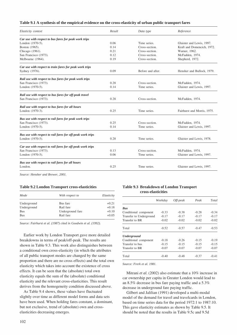
102

Earlier work by London Transport gave more detailedbreakdowns in terms of peak/off-peak. The results areshown in Table 9.3. This work also distinguishes betweena conditional own cross-elasticity (in which the attributesof all public transport modes are changed by the sameproportion and there are no cross effects) and the total ownelasticity which takes into account the existence of crosseffects. It can be seen that the (absolute) total ownelasticity equals the sum of the (absolute) conditionalelasticity and the relevant cross-elasticities. This resultderives from the homogeneity condition discussed above.

As Table 9.4 shows, these values have fluctuatedslightly over time as different model forms and data setshave been used. When holding fares constant, a dominant,but not exclusive, trend of (absolute) own and cross-elasticities decreasing emerges.

Mitrani et al. (2002) also estimate that a 10% increase incar ownership per capita in Greater London would lead toan 8.5% decrease in bus fare paying traffic and a 5.3%decrease in underground fare paying traffic.

Gilbert and Jalilian (1991) developed a multi-modalmodel of the demand for travel and travelcards in London,based on time series data for the period 1972:1 to 1987:10.This gave elasticity estimates as shown by Table 9.5. Itshould be noted that the results in Table 9.5c and 9.5d

Table 9.2 London Transport cross-elasticities

Mode With respect to Elasticity

Underground Bus fare +0.21Underground Rail fare +0.18Bus Underground fare +0.10Bus Rail fare +0.05

Source: Fairhurst et al. (1987) cited in Goodwin et al. (1992).

Table 9.1 A synthesis of the empirical evidence on the cross-elasticity of urban public transport fares

Elasticity context Result Data type Reference

Car use with respect to bus fares for peak work tripsLondon (1970-5). 0.06 Time series. Glaister and Lewis, 1997.Boston (1965). 0.14 Cross-section. Kraft and Domencich, 1972.Chicago (1961). 0.21 Cross-section. Warner, 1962.San Francisco (1973). 0.12 Cross-section. McFadden, 1974.Melbourne (1964). 0.19 Cross-section. Shepherd, 1972.

Car use with respect to train fares for peak work tripsSydney (1976). 0.09 Before and after. Hensher and Bullock, 1979.

Rail use with respect to bus fares for peak work tripsSan Francisco (1973). 0.28 Cross-section. McFadden, 1974.London (1970-5). 0.14 Time series. Glaister and Lewis, 1997.

Rail use with respect to bus fares for off-peak travelSan Francisco (1973). 0.28 Cross-section. McFadden, 1974.

Rail use with respect to bus fares for all hoursLondon (1970-3). 0.25 Time series. Fairhurst and Morris, 1975.

Bus use with respect to rail fares for peak work tripsSan Francisco (1973). 0.25 Cross-section. McFadden, 1974.London (1970-5). 0.14 Time series. Glaister and Lewis, 1997.

Bus use with respect to rail fares for off-peak work tripsLondon (1970-5). 0.28 Time series. Glaister and Lewis, 1978.

Car use with respect to rail fares for off-peak work tripsSan Francisco (1973). 0.13 Cross-section. McFadden, 1974.London (1970-5). 0.06 Time series. Glaister and Lewis, 1997.

Bus use with respect to rail fares for all hoursLondon. 0.25 Time series. Glaister and Lewis, 1997.

Source: Hensher and Brewer, 2001.

Table 9.3 Breakdown of London Transportcross-elasticities

Weekday Off-peak Peak Total

BusConditional component -0.33 -0.38 -0.28 -0.34Transfer to Underground -0.17 -0.17 -0.17 -0.17Transfer to BR -0.02 -0.02 -0.02 -0.02

Total -0.52 -0.57 -0.47 -0.53

UndergroundConditional component -0.18 -0.26 -0.15 -0.19Transfer to bus -0.15 -0.15 -0.15 -0.15Transfer to BR -0.07 -0.07 -0.07 -0.07

Total -0.40 -0.48 -0.37 -0.41

Source: Frerk et al. 1981.

103

have been restricted so as to be theoretically consistentwith the symmetry conditions discussed above.

Glaister (2001) has up-dated his earlier work (forexample, Glaister and Lewis, 1997) and producedestimates for London of a full set of cross-elasticities.These are shown by Table 9.6.

Mackett and Nash (1991) and Mackett and Bird (1989)have produced some estimates of the cross-elasticity ofcar, bus and walk trips to suburban rail journey time andfares. The results are given in Tables 9.7 and 9.8.

Mackett and Bird (1989) looked at rail fare cross-elasticities for car, bus and walk trips both in general andto central London. These results are given in Table 9.8:

9.2.2 Rest of Great BritainOutside London there has been limited work on publictransport cross-elasticities. However, some importantevidence has been collated on diversion rates. Thisevidence is summarised by Tables 9.9 and 9.10.

Outside London, some work has been undertaken whichinfers elasticities based on knowledge of diversion rates (as

given above), own elasticities and market shares. The ownelasticities and market shares are derived from meta-analyses of mode choice studies. The cross elasticities arethen inferred using the theoretical relationships outlined inSection 5.5. The earliest work in this area was by Acuttand Dodgson (1995) and is shown in Table 9.11. Somelater work by Wardman and colleagues is given in Tables9.12 and 9.13 for urban and interurban travel respectively.

One advantage of this approach is that it permits the useof elasticities from mode choice models. These are onlypartial estimates because they fail to take into accountdemand generation and suppression. The full elasticity ofdemand for mode i with respect to the price of mode jequals to the mode choice elasticity of the demand for iwith respect to the price of j plus the elasticity of totaltravel demand with respect the price of j (see, for example,Taplin, 1982). The latter can be estimated if the modechoice elasticity of j with respect to j’s own price isknown, along with the proportion of j’s additional demandthat is generated and j’s modal share.

A review by Dodgson (1990) found the most convincingcross elasticities of car use with respect to bus fares to be0.025 in London and 0.0105 in the six English metropolitancounties. Grayling and Glaister (2000) use a cross-elasticityof 0.09 for London, whilst Glaister uses values of rangingfrom 0.032 to 0.067 for the Metropolitan areas.

Table 9.4a London Underground models - priceelasticities (1995 fare levels)

R273 1971-85 M(97) 711971-95

Own price -0.49 -0.49Cross price elasticity, Bus +0.21 +0.20Cross price elasticity, BR +0.10 +0.08Conditional elasticity -0.19 -0.20

Table 9.4b London Underground models - priceelasticities (2000 fare levels)

M(97) 71 1971-95 1971-2000


Table 9.4c London bus models - price elasticities (1995fare levels)

R273 1971-85 M(97) 711971-95

Own price -0.71 -0.64Cross price elasticity, Underground +0.16 +0.13Cross price elasticity, BR +0.17 +0.16Conditional elasticity -0.40 -0.35

Table 9.4d London bus models - price elasticities (2000fare levels)

M(97) 71 1971-95 1971-2000


Sources: Fairhurst et al., 1987; London Transport, 1993a; Kincaid et al.,1997; Mitrani et al., 2002

Table 9.5a Estimated short-run price elasticities

Prices

Bus Underground British Rail Non-travel

Bus -0.839 0.476 0.082 0.281Underground 0.041 -0.355 0.160 0.114

Table 9.5b Estimated long-run price elasticities

Prices


Bus -1.318 0.897 0.193 0.229Underground 0.356 -0.688 0.211 0.120

Table 9.5c Estimated short-run price elasticities withlong-run symmetry imposed

Prices


Bus -0.788 0.414 0.096 0.278Underground 0.078 -0.396 0.182 0.058

Table 9.5d Estimated long-run price elasticities withlong-run symmetry imposed

Prices


Bus -1.185 0.724 0.240 0.221Underground 0.661 -0.983 0.166 0.156

104

Table 9.7 Cross-elasticities of car, bus and walk with respect to rail journey time

Mode Location Short run Medium run Long run

Car All trips from zones on the Chiltern Line. 0.07 0.06Bus All trips from zones on the Chiltern Line. 0.12 0.11Walk All trips from zones on the Chiltern Line. 0.05 0.05

Total All trips from zones on the Chiltern Line. 0.00 0.00

Car Trips to central London on the Chiltern Line. 0.37 0.18Bus Trips to central London on the Chiltern Line. 0.42 0.25Walk Trips to central London on the Chiltern Line. – –

Total Trips to central London on the Chiltern Line. -0.98 -1.13

Car All trips from zones in the south-east sector. 0.10 0.10Bus All trips from zones in the south-east sector. 0.14 0.14Walk All trips from zones in the south-east sector. 0.07 0.09

Total All trips from zones in the south-east sector. -0.00 -0.01

Car Trips to central London from zones in the south-east sector. 0.24 0.20Bus Trips to central London from zones in the south-east sector. 0.21 0.19Walk Trips to central London from zones in the south-east sector. 0.11 0.12

Total Trips to central London from zones in the south-east sector. -0.26 -0.34

Car All trips from zones on the Chiltern Line and south-east sector corridors. 0.10 0.11 0.11Bus All trips from zones on the Chiltern Line and south-east sector corridors. 0.21 0.21 0.21Walk All trips from zones on the Chiltern Line and south-east sector corridors. 0.07 0.08 0.08

Total All trips from zones on the Chiltern Line and south-east sector corridors. 0.00 0.00 0.00

Car Trips to central London on the Chiltern Line and south-east sector corridors. 0.95 0.97 0.96Bus Trips to central London on the Chiltern Line and south-east sector corridors. 0.91 0.94 0.94Walk Trips to central London on the Chiltern Line and south-east sector corridors. 0.60 0.67 0.68

Total Trips to central London on the Chiltern Line and south-east sector corridors. 0.00 0.00 0.00

Source: Mackett and Nash (1991) and Mackett and Bird (1989).

Table 9.8 Cross-elasticities with respect to rail fare

Elasticity

Mode All trips Trips to central London

Car 0.05 0.40Bus 0.10 0.36Walk 0.03 0.25

Source: Mackett and Bird (1989)

Table 9.6 Matrix of cross-elasticities for London

Under-Bus ground Rail Caruse use use use

Bus fare – 0.13 0.06 0.04Underground fare 0.06 – 0.03 0.02Rail fare 0.11 0.06 – N/CBus miles – 0.22 0.10 0.09Underground miles 0.09 – 0.04 0.03Bus journey time – 0.18 0.08 0.06

Source: Glaister, 2001.

105

Table 9.9 Diversion rates (%) - urban

From

Cycle Gener No. ofTo Rail Bus Car /Walk -ated studies

Rail – 41 33 1 24 4Bus 6 – 31 42 21 2Car 24 48 – 6 22 1

Sources: Vicario, 1999, Chartered Institute of Transport, 1996, Centro,1998, 1999, MVA, 2000a.

Table 9.10 Diversion rates (%) - interurban

From

Gener No. ofTo Rail Coach Car Air -ated studies

Rail – 20 60 6 14 2Coach 60 – 22 – 18 1Car 42 10 – 1 47 1

Sources: Vicario, 1999, Gordon (2000).

Table 9.11 Deduced public transport and carcross-elasticities

PT use with respect Car use with respectMarket to petrol price to PT fares

Inter city 0.0939 0.0118Network SE 0.0409 0.0026Regional rail 0.0909 0.0022London underground 0.0171 0.0006London buses 0.0199 0.0005Other local buses 0.0132 0.0018

Source: Acutt and Dodgson (1995)

Table 9.12 Deduced cross-elasticities – urban

Car use Rail use Bus use

Car cost – 0.59 0.55Rail cost 0.054 – 0.08Bus cost 0.057 0.24 –

Sources: Toner (1993), Wardman (1997b).

Table 9.13 Deduced cross-elasticities – interurban

Car use Rail use Coach use

Car time – 0.33 0.60Car cost – 0.25 0.34Rail time 0.057 – 0.20Rail cost 0.066 – 0.32Coach time 0.054 0.17 –Coach cost 0.014 0.17 –

Source: Wardman (1997a).

Table 9.14 Stated intentions responses to road pricing

Method of charging

Distance-based Cordon-basedResponse (1260 respondents) (585 respondents)

Pay charge 42.0% 45.3%Shift to earlier time 13.6% 11.9%Shift to later time 4.1% 2.8%Use public transport 16.1% 16.1%Use car and PT 3.6% 4.3%Cycle or walk 5.3% 3.5%Switch route 4.2% 5.1%Change destination 5.0% 4.1%Other 6.1% 6.9%

Source: Polak et al. (1993).

Table 9.15 Cross-elasticity of demand for car withrespect to bus fare

Route type Cross-elasticity

Large radial 0.018Orbital 0.026Medium radial 0.027Park and ride 0.097Small radial 0.045Inter-urban 0.008Rural radial 0.026

Polak et al. (1993) use the stated intentions technique toexamine short-term responses to the introduction of roadpricing. These are shown in Table 9.14. The report alsoassesses longer term impacts, allowing for ‘lifestyle impacts’.

Recent work undertaken for the Commission forIntegrated Transport has estimated the cross-elasticity ofthe demand for car travel with respect to bus price basedon a 10% bus fare increase (Institute for Transport Studiesand Transport Studies Unit 2002). The results are shown inTable 9.15.

Work in the passenger rail market by Steer DaviesGleave (1999a) has inferred a series of urban andinterurban cross-elasticities. These values have been usedin the Rail Industry Forecasting Framework (RIFF) andversion 4 of the Passenger Demand Forecasting Handbook.They are shown in Tables 9.16 and 9.17.

Finally, some illustrative examples are reported to revealthe principle of cross-elasticity estimation. Such an exerciseis based on the review of car price elasticity carried out byHanly et al. (2002). They conducted a literature review ofprice and income elasticities in the demand for road traffic.The data used in the review consist of the results of 69different published elasticity studies. The comprehensivework by Hanly et al. (2002) provides us with a ground forthe inference of cross-elasticities with respect to car fuelprices. Combining Hanly et al. (2002) findings with thediversion rate figures from Tables 9.9 and 9.10 as well asthe relative market share data from Department of theEnvironment, Transport and the Regions (1999), we are ableto derive the relevant public transport cross-elasticity withrespect to car price (fuel costs).

Preston and Wardman (1991) report the arc-elasticity ofcar use with respect to bus cost changes of between 10%and 300% as being 0 to 0.33. This was based on transferprice questions, adjusted for non-traders.

106

Table 9.18 reports the short-term bus and rail elasticitywith respect to fuel costs. It is estimated based onformula (17) (Section 5.5). It shows that the cross-elasticities with respect to fuel price are higher for urbanbus and inter-urban rail, which is mainly due to the higherdiversion rate for these two segments.

Table 9.16 Cross-elasticities of urban rail demand

Bus UnderFuel Car Bus Bus head -groundcost time cost time -way cost

London Travelcard areaCommuting 0.2 0.1 0.1 0.05 0.025 0.1Business 0.2 0.1 0.0 0.0 0.0 0.0Leisure 0.2 0.1 0.2 0.05 0.025 0.2

S.E. to LondonSeason 0.0 0.0 0.0 0.0 0.0 –Daily 0.19 0.24 0.17 0.17 0.03 –

S.E. from LondonSeason 0.25 0.30 0.20 0.20 0.05 –Daily 0.24 0.30 0.20 0.20 0.03 –

S.E. non LondonSeason 0.25 0.30 0.20 0.20 0.05 –Daily 0.24 0.30 0.20 0.20 0.03 –

R.O.C. to London (< 100 Miles)First 0.12 0.30 0.00 0.00 0.00 –Full 0.18 0.30 0.12 0.12 0.02 –Reduced 0.25 0.30 0.23 0.23 0.04 –

Total 0.22 0.30 0.18 0.18 0.03 –

Non London (<20 miles)Season 0.30 0.25 0.20 0.15 0.025 –Daily 0.34 0.25 0.22 0.14 0.025 –Pre-paid 0.40 0.20 0.30 0.10 0.05 –

S.E. = south east, R.O.C. = Rest of CountrySource: Rail Industry Forecasting Framework as in PDFH version 4.

Table 9.17 Interurban rail demand cross-elasticities

Bus AirFuel Car Bus Bus head Air headcost time cost time -way cost -way

R.O.C. to London (200 m +) 1st 0.12 0.30 0.00 0.00 0.00 0.25 0.05Full 0.18 0.30 0.12 0.12 0.02 0.25 0.05Reduced 0.25 0.30 0.23 0.23 0.04 0.25 0.05

Total 0.22 0.30 0.18 0.18 0.03 0.25 0.05

Non London1

20-100m 0.27 0.30 0.17 0.17 0.04 0.25 0.05100-200m 0.27 0.30 0.17 0.17 0.04 0.25 0.05200m + 0.27 0.30 0.17 0.17 0.04 0.25 0.05

Non London2

1st 0.12 0.30 0.00 0.00 0.00 0.25 0.05Full 0.18 0.30 0.12 0.12 0.02 0.25 0.05Reduced 0.25 0.30 0.23 0.23 0.04 0.25 0.05

Total 0.20 0.30 0.13 0.30 0.03 0.25 0.05

Airports0.25 0.30 0.10 0.10 0.03 – –

1 Over 20 miles, less than 10% using first and full tickets.2 Over 20 miles, more than 10% using first and full tickets.

R.O.C = Rest of country.

Source: Rail Industry Forecasting Framework as in PDFH version 4.

Table 9.18 Short-term public transport cross-elasticitywith respect to fuel costs

Cross Car Diversionelasticity elasticity Relative rate

with respect with respect market share (from PTto fuel price to fuel price (car/PT mode) mode to car)

Urban rail 0.35 -0.10 14.40 0.24Urban bus 0.72 -0.10 15.10 0.48Inter rail 0.60 -0.10 14.40 0.42Inter coach 0.15 -0.10 15.10 0.10

Source: Estimates based on Hanly et al. (2002).

Table 9.19 Long-term public transport cross-elasticitywith respect to fuel costs

Cross Car Diversionelasticity elasticity Relative rate

with respect with respect market share (from PTto fuel price to fuel price (car/PT mode) mode to car)

Urban rail 1.00 -0.29 14.40 0.24Urban bus 2.10 -0.29 15.10 0.48Inter rail 1.75 -0.29 14.40 0.42Inter coach 0.44 -0.29 15.10 0.10

Source: Estimates based on Hanly et al. (2002).

Table 9.19 reports the long-term public transport cross-elasticity with respect to fuel costs. The estimated cross-elasticity values are rather high, suggesting strong effectsof car costs on public transport use in the long run.Nevertheless, the examples given here are regarded asillustrative rather than definitive, as the car price elasticityand relative market share do not distinguish between urbanand inter-urban journeys.

9.2.3 Evidence from abroadThere is evidence on cross-elasticities from abroad,particularly Australia. For example, Johnson and Hensher(1982) developed a Multinomial Probit model ofpassengers’ choices between car and train. This model wascalibrated on panel data collected in the suburbs ofSydney, between 1971-73 for 163 observations. Elasticityestimates were based on PC, the probability of choosingcar, and PT, the probability of choosing train. The resultsare shown in Table 9.20.

Hensher (1997) estimated cross-elasticities betweenticket-types and between modes (rail, bus, and car) forcommuters in Sydney. The elasticity matrix is shown inTable 9.21. This table indicates how changes in varioustypes of transit fares and car operating costs affect the use ofother types of transit fares and car travel. This is based on asurvey of residents of Newcastle, a small Australian city.

107

Hensher (1998) noted that previous studies whichevaluated and modelled modal choice in terms of anaverage fare ignored the reality of ticket-switching withinthat mode. However, on modelling using ticket types, itwas found that people were more likely to switch modethan ticket. This was contrary to a priori expectations.

In terms of commuter travel, Taplin et al. (1997) cited inthe Australian Bureau of Transport Economics (2001),have provided optimally adjusted elasticities for travel byvarious modes in Sydney, as shown in Table 9.22.

the competition is stronger. Road is generally faster thanrail in Spain, although there are exceptions (for instancethe Madrid – Seville AVE high-speed train).

TRACE (1999) provides detailed elasticity and cross-elasticity estimates for various types of travel (car-trips,car-kilometres, transit travel, walking/cycling, commuting,business, etc.) and conditions, based on numerousEuropean studies. The findings of the TRACE project aresummarised in De Jong and Gunn (2001). Table 9.23reports the impact of car costs and car time on publictransport. The cross-elasticities for the number of publictransport trips and public transport kilometres travelledwith respect to each explanatory variable are reported. Theelasticities with respect to fuel price in general turn out tobe quite small, with long run values of around 0.1. The cartime has a greater impact on public transport demand, withaverage long run elasticity of 0.25.

Table 9.20 Car and rail own and cross-elasticities,Sydney, Australia

Model

DS73DS73 Sequen Auxil

DS71 DS71 DS73 Dummy -etial Naive -iaryElasticity Logit Probit Probit linkage linkage pooling pooling

PC/invtC

-0.400 -0.445 -0.609 -0.556 -0.625 -0.533 -0.109PC/invt

T+0.665 +0.467 +0.642 +0.605 +0.658 +0.562 +0.120

PC/costC

-1.260 -0.971 -0.387 -0.255 -0.383 -0.622 -0.119PC/cost

T+1.780 +0.612 +0.312 +0.199 +0.386 +0.449 +0.085

PT/invtC

+0.905 +0.418 +0.859 +0.823 +0.899 +0.627 +0.108PT/invt

T-0.387 -0.439 -0.905 -0.880 -0.947 -0.662 -0.119

PT/costC

+1.52 +0.911 +0.546 +0.371 +0.552 +0.733 +0.118PT/cost

T-0.751 -0.574 -0.440 -0.290 -0.441 -0.529 -0.084

Table 9.21 Direct and cross-share elasticities forSydney, Australia

Train Train Train Bus Bus Bus Car

Single Ten Single Tenfare fare Pass fare fare Pass

Train, single fare -0.218 0.001 0.001 0.057 0.005 0.005 0.196Train, ten fare 0.001 -0.093 0.001 0.001 0.001 0.006 0.092Train, pass 0.001 0.001 -0.196 0.001 0.012 0.001 0.335Bus, single fare 0.067 0.001 0.001 -0.357 0.001 0.001 0.116Bus, ten fare 0.020 0.004 0.002 0.001 -0.160 0.001 0.121Bus, pass 0.007 0.036 0.001 0.001 0.001 -0.098 0.020Car 0.053 0.042 0.003 0.066 0.016 0.003 -0.197

Table 9.22 Optimally adjusted commuter elasticitiescondensed to modes

Elasticity with respect to fare or cost of trip

Travel mode Train Bus Ferry Car

Train -0.156 0.032 0.003 0.037Bus 0.063 -0.070 0.006 0.046Ferry 0.039 0.037 -0.195 0.003Car 0.016 0.011 0.000 -0.024

A recent study of inter-urban transport in Spain (Coto-Millan et al., 1997) reported short term cross-elasticitiesfor rail demand (millions of passengers per km of route)with respect to the price of petrol of 0.74 for Talgo (fast)trains, and 0.56 for standard trains. These results conformto the expectations that elasticities should be higher where

Table 9.23 Cross-elasticity of public transport demandwith respect to car costs and car time

Explained Explanatory Short run Long run

PT trips Fuel price 0.33 0.07PT kms Fuel price 0.07 0.10PT trips Car time 0.27 0.15PT kms Car time 0.52 0.36

Source: De Jong and Gunn, 2001.

Table 9.24 Cross-elasticity of public transport demandwith respect to car costs by journey purpose

Journey purpose Explained: PT trips Explained: PT kms

Commuting 0.20 0.22Business 0.24 0.05Education 0.01 0.00Other 0.15 0.18

Total 0.13 0.14

Source: TRACE (1999) cited in Litman (2002)

The public transport elasticity with respect to car costsalso varies with journey types. The results from theTRACE project shows that in general the public transportdemand with respect to car costs is most elastic forcommuting but least elastic for education journeys. Table9.24 summarizes elasticities of trips and kilometres withrespect to fuel prices in areas with high vehicle ownership(more than 450 vehicles per 1,000 population).

There is also a body of international evidence ondiversion rates (see, for example, Booz Allen andHamilton, 1999). This evidence is context specific andrequires careful interpretation. Table 9.25 summarisessome international evidence for urban rail schemes.Overall, this work suggests on average that around 66% ofthe use of new urban rail schemes comes from existingpublic transport with 17% coming from car, 10%generated and 7% coming from other sources (cycling andwalking). In part these diversion rates will be determined

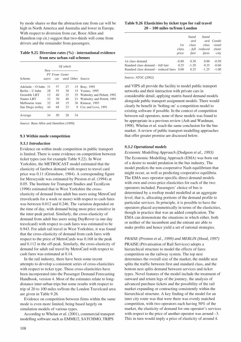
108

by mode shares so that the abstraction rate from car will behigh in North America and Australia and lower in Europe.With respect to diversion from car, Booz Allen andHamilton (op cit.) suggest that two-thirds will come fromdrivers and the remainder from passengers.

and VIPS all provide the facility to model public transportnetworks and their interaction with private cars inconsiderable detail, applying matrix-based demand modelsalongside public transport assignment models. There wouldclearly be benefit in ‘bolting on’ a competition model toexisting software if possible. In the context of competitionbetween rail operators, none of these models was found tobe appropriate in a previous review (Ash and Wardman,1998). Whelan et al. reach the same conclusion for the busmarket. A review of public transport modelling approachesthat offer greater promise are discussed below.

9.3.2 Operational modelsEconomic Modelling Approach (Dodgson et al., 1993)The Economic Modelling Approach (EMA) was born outof a desire to model predation in the bus industry. Themodel predicts the non-cooperative Nash equilibrium thatmight occur, as well as predicting cooperative equilibria.The EMA uses operator-specific direct demand modelswith own and cross-price elasticities for each of the twooperators included. Passengers’ choice of bus isdetermined by a rooftop model modelled at an aggregatelevel, that is, allocating portions of the demand profile toparticular services. In principle, it is possible to have theoperators placed asymmetrically in terms of the elasticities,though in practice that was an added complication. TheEMA can demonstrate the situations in which either, bothor neither of the incumbent and the entrant are able tomake profits and hence yield a set of rational strategies.

PRAISE (Preston et al., 1999) and MERLIN (Hood, 1997)PRAISE (Privatisation of Rail Services) adopts ahierarchical structure to model the effects of farescompetition on the railway system. The top nestdetermines the overall size of the market, the middle nestsplits the traffic between first and standard class, and thebottom nest splits demand between services and tickettypes. Novel features of the model include the treatment ofoutward and return legs of the journey, the analysis ofadvanced purchase tickets and the possibility of the railmarket expanding or contracting consistently within thehierarchical structure. A key finding of the model for aninter city route was that were there was evenly matchedcompetition, with two operators each having 50% of themarket, the elasticity of demand for one operator’s serviceswith respect to the price of another operator was around –3.This in turn would imply a price of elasticity of around 4.

Table 9.25 Diversion rates (%) - international evidencefrom new urban rail schemes

Of whichNew

PT From GenerScheme users car -ated Other Source

Adelaide – O bahn 31 57 27 15 Bray, 1995Berlin – U bahn 28 55 30 15 Younes, 1995Grenoble LRT 12 40 25 35 Walmsley and Pickett, 1992Nantes LRT 33 30 48 21 Walmsley and Perrett, 1991Melbourne tram 32 49 15 36 Kinnear, 1993San Diego trolley 44 68 23 9 Cox and Love, 1991

Average 34 50 28 34

Source: Booz Allen and Hamilton (1999).

Table 9.26 Elasticities by ticket type for rail travel20 – 100 miles to/from London

Stand Stand-ard -ard Condit

1st class class -ionalclass - full -reduced elastiprice fare fares -city

1st class demand -0.80 0.30 0.00 -0.50Standard class demand – full fare 0.25 -1.20 0.35 -0.60Standard class demand – reduced fares 0.00 0.25 -1.25 -1.00


9.3 Within mode competition

9.3.1 IntroductionEvidence on within mode competition in public transportis limited. There is some evidence on competition betweenticket types (see for example Table 9.22). In WestYorkshire, the METROCAST model estimated that theelasticity of farebox demand with respect to travel cardprice was 0.11 (Grimshaw, 1984). A corresponding figurefor Merseyside was estimated by Preston et al. (1994) at0.05. The Institute for Transport Studies and TecnEcon(1996) estimated that in West Yorkshire the cross-elasticity of demand from adult bus users using MetroCard(travelcards for a week or more) with respect to cash fareswas between 0.012 and 0.246. The variation depended onthe time of day, with demand being most price sensitive inthe inter-peak period. Similarly, the cross-elasticity ofdemand from adult bus users using DayRover (a one daytravelcard) with respect to cash fares was estimated to be0.943. For adult rail travel in West Yorkshire, it was foundthat the cross-elasticity of demand from cash fares withrespect to the price of MetroCards was 0.168 in the peakand 0.112 in the off-peak. Similarly, the cross-elasticity ofdemand for adult rail travel by MetroCard with respect tocash fares was estimated at 0.14.

In the rail industry, there have been some recentattempts to develop a consistent series of cross-elasticitieswith respect to ticket type. These cross-elasticities havebeen incorporated into the Passenger Demand ForecastingHandbook, version 4. Most of the estimates relate to long-distance inter-urban trips but some results with respect totrip of 20 to 100 miles to/from the London Travelcard areaare given in Table 9.26.

Evidence on competition between firms within the samemode is even more limited, being based largely onsimulation models of various types.

According to Whelan et al. (2001), commercial transportmodelling software such as EMME/2, SATCHMO, TRIPS

109

The cost model adopted was essentially an accounting-based approach in order to achieve fully allocated costs.There is separate identification of operating and capitalcosts and both types of cost are composed of both fixedand variable elements. The outputs of PRAISE can bechecked to see if the effects of changes in prices orservices accord with external evidence. The competitivestrategies which can be modelled include: cream-skimming; head-on competition with service matching;price wars; and product differentiation. MERLIN (Modelto Evaluate Revenue and Loadings for Intercity) has asimilar demand structure to PRAISE but with thegeneration/suppression effects being incorporated byapplication of known market elasticities to changes inaverage fares and generalised times.

Quality bus model (Whelan et al., 2001)

This model was designed to provide information to beused to:

� determine demand and cost implications of Quality BusPartnerships (QBPs);

� assess the likelihood of market entry and exit;

� evaluate pricing, service level and quality of servicestrategies; and

� undertake an economic evaluation.

The model has a degree of flexibility so that it can beapplied to a range of possible QBP scenarios. In the firstinstance, the spatial and temporal dimensions of the modelare described. This is followed by an outline of thedemand and cost models and finally the way in which thedemand and cost models can be linked and dynamicsadded to the system is examined.

The model structure is simple but flexible enough todeal with a variety of QBP arrangements. Working on theassumption that there exist well-defined corridors thatform the basis for operator strategies the model consists ofa series of n zones, with j parallel bus routes runningthrough each zone. Demand for travel between any twozones in the network is then allocated to availableindividual services (e.g. the 0704 departure from zone 2 onroute 1) according to the sensitivity of demand to thegeneralised cost of travel and the socio-economiccharacteristics of the travellers.

The temporal aspects of the model are constrained, byand large, by the availability of base input data. Forexample, if data on base demand levels are only availableas daily totals there is little point in trying to model thespread of traffic throughout the day. The default timescalefor the model is set to be a representative one-hour period.Here, the analyst can run the model for key hour periodsduring the day/week/season and gross-up the estimates togive weekly or annual totals. With relatively minorchanges to the source code, the model can be set up tocover any time period desired. A key requirement of themodel is that it should be able to predict year roundprofitability. Applications of the model should thereforetake account of seasonality.

The purpose of the demand model is firstly to determinethe overall size of the bus market and secondly to divide themarket between operators, ticket types and departure times.This information can then be combined with fare data togenerate forecast revenues. It has been assumed that theindividual is the decision-making unit and that all decisionsare taken at ‘point of sale’. Using decision rules based onutility maximisation, a given individual has to consider:

� whether or not to make the journey; and

� which mode to use.

If they choose to make a journey and travel by bus, thefollowing additional considerations are of interest:

� which stop to board at and alight from (if available);

� which operator to travel with (if available);

� which service to use (time of departure); and

� which ticket type to use.

The interrelated choices set out above can berepresented in a range of demand models, from modelswith complex hierarchical structures to relatively simpledirect demand models. Our preferred approach makes thebest use of documented evidence on bus passengers’valuations of journey attributes (e.g. in-vehicle time) andsensitivities to changes in costs and involves a two levelchoice model:

� Level 1 - Choice of service (route, departure-time,operator and ticket type).

� Level 2 - Choice of mode (including not travel).

This structure allows for the allocation of passengersbetween operators, ticket types and services and for theoverall size of the bus market to expand or contract asservice levels change.

The way in which the model is applied is outlined below:

i For each OD pair on the network in a given operationalperiod (e.g. a peak hour), generate a sample of, say, 500individuals with a given distribution of tastes (attributevalues), characteristics (e.g. child, adult, pensioner) andmost preferred departure times.

ii For each individual, estimate the generalised cost ofeach service and ticket type available and select the bestn options. Each of these is then allocated a probabilityby level 1 of the model with all other options assigned azero probability.

iii The market shares for each service and ticket type (for agiven OD pair in a given operational period) are thenestimated by averaging the derived probabilities over all500 individuals.

iv The overall size of the bus market (total number ofpassengers for a given OD pair in a given operationalperiod) is then determined in Level 2 of the model andsubsequently assigned to individual services usingmarket share estimates.

On this basis, total demand and revenue estimates can bederived for each service and ticket type. Where servicesare estimated to reach capacity, service levels areautomatically increased through the use of duplicatedvehicles.

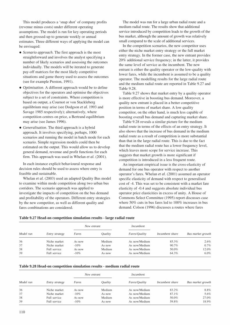
110

This model produces a ‘snap shot’ of company profits(revenue minus costs) under different operatingassumptions. The model is run for key operating periodsand then grossed-up to generate weekly or annualestimates. Three different ways of applying the model canbe envisaged:

� Scenario approach. The first approach is the moststraightforward and involves the analyst specifying anumber of likely scenarios and assessing the outcomesindividually. The models will be iterated to generatepay-off matrices for the most likely competitivesituations and game theory used to assess the outcomes(see for example Preston, 1991).

� Optimisation. A different approach would be to defineobjectives for the operators and optimise the objectivessubject to a set of constraints. Where competition isbased on output, a Cournot or von Stacklebergequilibrium may arise (see Dodgson et al. 1993 andSavage 1985 respectively); alternatively, wherecompetition centres on price, a Bertrand equilibriummay arise (see James 1996).

� Generalisation. The third approach is a hybridapproach. It involves specifying, perhaps, 1000scenarios and running the model in batch mode for eachscenario. Simple regression models could then beestimated on the output. This would allow us to developgeneral demand, revenue and profit functions for eachfirm. This approach was used in Whelan et al. (2001).

In each instance explicit behavioural response anddecision rules should be used to assess where entry isfeasible and sustainable.

Whelan et al. (2003) used an adapted Quality Bus modelto examine within mode competition along two urban buscorridors. The scenario approach was applied toinvestigate the impacts of competition on the bus demandand profitability of the operators. Different entry strategiesby the new competitor, as well as different quality andfares combinations are considered.

The model was run for a large urban radial route and amedium radial route. The results show that additionalservice introduced by competition leads to the growth of thebus market, although the amount of growth was relativelysmall compared to the scale of additional services.

In the competition scenarios, the new competitor useseither the niche market entry strategy or the full marketentry strategy. In the former case, the new entrant provides20% additional service frequency; in the latter, it providesthe same level of service as the incumbent. The newentrant is either the quality operator or the low-quality withlower fares, while the incumbent is assumed to be a qualityoperator. The modelling results for the large radial routeand the medium radial route are reported in Table 9.27 andTable 9.28.

Table 9.27 shows that market entry by a quality operatoris more effective in boosting bus demand. Moreover, aquality new entrant is placed in a better competitiveposition in terms of market share. A low qualitycompetitor, on the other hand, is much less capable ofboosting overall bus demand and capturing market share.

Table 9.28 reveals a similar picture for the mediumradial route in terms of the effects of an entry strategy. Italso shows that the increase of bus demand in the mediumradial route as a result of competition is more substantialthan that in the large radial route. This is due to the factthat the medium radial route has a lower frequency level,which leaves more scope for service increase. Thissuggests that market growth is more significant ifcompetition is introduced in a less frequent route.

An important empirical issue is the cross-elasticity ofdemand for one bus operator with respect to anotheroperator’s fares. Whelan et al. (2001) assumed an operatorspecific elasticity of demand with respect to generalisedcost of -4. This was set to be consistent with a market fareelasticity of -0.4 and suggests absolute individual busoperator price elasticities in excess of unity. A House ofCommons Select Committee (1995) report discusses casewhere 50% cuts in bus fares led to 100% increases in busdemand. Colson (1996) discusses a routes where fares

Table 9.27 Head-on competition simulation results - large radial route

New entrant Incumbent

Model run Entry strategy Fares Quality Fares/Quality Incumbent share Bus market growth

36 Niche market As now Medium As now/Medium 85.3% 2.6%37 Niche market -10% As now As now/Medium 90.7% 0.7%38 Full service As now Medium As now/Medium 50.0% 12.0%39 Full service -10% As now As now/Medium 64.3% 6.0%

Table 9.28 Head-on competition simulation results - medium radial route

New entrant Incumbent

Model run Entry strategy Fares Quality Fares/Quality Incumbent share Bus market growth

36 Niche market As now Medium As now/Medium 83.2% 8.8%37 Niche market -10% As now As now/Medium 87.1% 5.6%38 Full service As now Medium As now/Medium 50.0% 27.0%39 Full service -10% As now As now/Medium 59.8% 18.9%

111

were halved and ridership increased by 275%. However, inboth cases these demand changes occurred in competitivesituations and reflect operator-specific effects. Theseresults suggest operator-specific arc elasticities of around-1.0 and -2.2 respectively. Assuming a market fareselasticity of -0.4, this would imply cross-elasticities of 0.6and 1.8 respectively.


Dargay and Hanly (1999) conclude that, although theempirical evidence is limited, bus fares appear to havenegligible effects on car travel. The effects of motoringcosts on bus travel, however, are slightly greater. Theybelieve that the cross-elasticity between bus patronageand motoring costs appears to be negligible in the shortrun, and about 0.3 to 0.4 in the long run. Clearly, there isa price-substitution between bus and car use, althoughcomparatively small. We must keep in mind that theseelasticities were estimated over a period in which busfares rose substantially in comparison to motoring costs,and an opposite development need not produce anequivalent impact.

Oum et al. (1992) conclude that it is important that amode’s demand specifications include the prices andquality of service of competing modes. Because somestudies do not take into account intermodal competition,their elasticity estimates may partly reflect the intensity ofintermodal competition, and as a result underestimate theown-price elasticity if the competing modes have changedtheir prices in the same direction.

Acutt and Dodgson (1995) state: ‘..... any cross-elasticity estimates from one study will not be directlyapplicable to another because the cross-elasticity valuesdepend on the relative size of the two marketsrepresented’. We therefore avoid recommending a singleset of cross-elasticity values for urban travel. A partialexception is London where a number of cross elasticitieshave been estimated. These are summarised by Tables 9.29and 9.30.

The studies in Table 9.29 also found a cross-elasticity ofcar use with respect to rail fare in the range 0.05 to 0.40,with corresponding cross elasticities for bus use and walkin the range 0.10 to 0.36 and 0.03 to 0.25 respectively. Thehigh cross elasticities refer to trips to/from central Londonwhere rail has a high market share.

Overall, it is concluded that there is less evidence oncross-elasticities than direct elasticities, particularly interms of dynamic studies. In part, this reflects estimationproblems and means that cross elasticities will often haveto be inferred. With the exception of trips to centralLondon, it might be expected that the cross-elasticity ofcar demand with respect to public transport attributes islow, although non-zero. The cross-elasticity of publictransport demand with respect to car attributes might beexpected to be more substantial. Similarly, the cross effectsbetween public transport modes can be substantial.

The various models that have been developed toexamine this issue have been reviewed. Particular attentionhas been paid to the PRAISE and MERLIN models thatinform the rail Passenger Demand Forecasting Handbook

and the QBP (Quality Bus Partnership) model that hasbeen used recently to examine bus subsidy options. It hasbeen noted that there is limited empirical evidence onoperator specific own- and cross-elasticities.

10 Effects of income and car ownership

10.1 Introduction

This chapter deals with the effects of income and carownership upon the demand for public transport.Traditionally these variables have been deemed‘background factors’, as compared to the endogenousfactors within public transport such as fares, service levels,journey times and vehicle quality. The broad relationshipsbetween these factors and the demand for public transportare well documented, but despite this the exactrelationships and the correlation between all three factors,and in particular between income and car ownership,would appear to be only marginally clearer 23 years onfrom the 1980 Demand for Public Transport publication.

The last 23 years have seen marked increases in realincome and car ownership levels in the UK and acrossEurope. For example, in this period GDP increased byaround 68% in Great Britain whilst the number of cars perhousehold increased from 0.76 to 1.11. In that time, localbus journeys have fallen by around a third. The position forrail is more mixed. The performance of rail at a local leveldepends on congestion levels and, because of the perceived

Table 9.29 Summary of cross-elasticities forLondon – fares

Numberof

observaDemand With respect to Mean Range -tions

Bus - short run Underground price 0.45 0.41 – 0.48 2Bus - long run Underground price 0.57 0.10 – 0.90 3Bus - short run BR price 0.09 0.08 – 0.10 2Bus - long run BR price 0.18 0.17 – 0.19 2Underground - short run Bus price 0.06 0.04 – 0.08 2Underground - long run Bus price 0.41 0.20 – 0.66 3Underground - short run BR price 0.11 0.04 – 0.20 3Underground - long run BR price 0.51 0.36 – 0.66 2

Sources: Fairhurst et al. (1987), Gilbert and Jalilian (1991).

Table 9.30 Summary of cross-elasticities for London –journey time

Numberof

observaDemand With respect to Mean Range -tions

Car - short run Rail journey time 0.30 0.07 – 0.95 6Car - long run Rail journey time 0.27 0.06 – 0.96 6Bus - short run Rail journey time 0.34 0.12 – 0.91 6Bus - long run Rail journey time 0.31 0.11 – 0.94 6Walk - short run Rail journey time 0.15 0 – 0.60 6Walk - long run Rail journey time 0.17 0 – 0.67 6

Sources: Mackett and Bird (1989), Mackett and Nash (1991).

112

higher quality of rail, is less sensitive to increases in carownership than bus. Indeed, central London rail commutertraffic has increased by 13% since 1980.

Income is expected to increase the number of trips andtheir average length. It is likely that this additional travelwill be split between increased public transport trips andincreased car trips, depending upon the level of caravailability and assuming that public transport is a normalgood. Income is also a key determinant of car ownershipand hence there will be a secondary and negative impacton the demand for public transport via car ownership.

In contrast to the marked impacts of income and carownership, the impact of socio-economic factors is likely tobe less dramatic. Although trip making patterns varysubstantially with socio-demographics, changes indemographics and household sizes are very much long termin nature and as such are less significant in terms of changesin travel over time. However, results presented here indicatethat these factors may be very important in explainingdifferences in trip making patterns between areas.

Other chapters in this document categorise the empiricalevidence according to whether it is obtained fromaggregate or disaggregate models. Given thecomparatively few studies in this area, such a distinctiondoes not here seem sensible and evidence from bothsources is taken together. Moreover, the nature of theeffects considered in this chapter is such that the empiricalevidence is firmly based upon actual behaviour rather thanresponses to hypothetical questions of one form or another.

The structure of this chapter is as follows. Section 10.2outlines the effects of income and car ownership on thedemand for public transport from a theoretical perspectiveand discusses the practical problems involved in

disentangling the separate effects of each. Section 10.3considers the evidence relating to the impact of income ontravel expenditure and distance travelled. The empiricalevidence relating to the effect of income on public transportdemand is discussed in Section 10.4, followed byconsideration of the effect of car ownership on the demandfor public transport in Section 10.5. Studies which haveaddressed both income and car ownership simultaneouslyare reviewed in Section 10.6 whilst Section 10.7 speculatesas to how the effect of income changes on the demand forpublic transport may vary over time. A summary andconcluding remarks are provided in Sections 10.8 and 10.9.

10.2 The expected effects of income and car ownershipon public transport demand

Potter et al. (1997) have identified rising car and licenceownership, income growth and the declining real cost ofcar ownership as the key factors that have shaped personaltravel patterns in the last twenty years. Whilst a host ofother background factors can be cited (see Figure 10.1)four key relationships are outlined below that underpin therest of the discussion in this chapter:

� An increase in income will, depending upon the level ofincome, lead to an increase in car ownership and so caravailability, or to an increase in public transport use (arelationship missed out in Figure 10.1).

� An increase in car ownership/availability will, otherthings being equal, lead to a reduction in the demand forpublic transport modes.

� The sign and magnitude of demand elasticities forpublic transport with respect to car availability andincome will vary depending upon the income levels.

INCOME

SETTLEMENTSIZE, DENSITY

& CONFIGURATION

HOUSEHOLDCHARACTERISTICS

CAR OWNERSHIP

TRIP LENGTH NUMBEROF

TRIPS

CAR USE PUBLICTRANSPORT

USE

WALK&

CYCLE

CULTURE,ATTITUDES &

PERCEPTIONS

HomeLocation

Distributionof facilities

Vehicle Cost

Congestion LicenseOwnership

Fuel Cost

Fares &ServiceQuality

Figure 10.1 Linkages between factors affecting trip generation and modal choice(Source: Potter et al., 1997)

113

� Income growth can be expected to increase average triplength, in part alongside changing patterns of land usebut also independently of them.

The relationships discussed above for the greater partmean that considerable care must be taken wheninterpreting public transport demand elasticities that havebeen estimated with respect to income and car ownership.Income elasticities estimated using demand models that donot have car ownership amongst their explanatoryvariables will pick up the negative effect that carownership has on public transport. This could lead toresults which contradict the ‘accepted thinking’ that publictransport is not an inferior good. The problem withestimating models that include both variables is thecollinearity that exists between them. The first Demand forPublic Transport book noted this in detail and twenty yearson the problem of collinearity still exists and is particularlynoticeable for models that have been calibrated using timeseries data.

To illustrate the problem of disentangling the effects ofincome and car ownership, various models were estimatedto rail ticket sales data (CAPRI) for journeys on non-season tickets in the south east as part of an update to thePassenger Demand Forecasting Handbook (ATOC, 2002).The ticket sales related to annual trips covering the years1991 to 1999 between a wide range of stations.

The results are given in Table 10.1. Separate GDPelasticities are reported for trips to London, trips fromLondon and other trips within the south east. NCO denotesthe proportion of households without a car. It is specifiedto influence rail demand (V) as:

NCOV eβ=

The elasticity of rail demand with respect to NCO istherefore βNCO which falls as NCO falls and carownership tends to saturation. Fuel and car time denotecross elasticities of rail demand with regard to the costsand times involved in using car. A Department forTransport fuel price index was used for fuel cost whilstassumptions were made about car journey time increasesover the period.

Where a parameter is freely estimated, its 95%confidence interval is given in brackets. The absence of aconfidence interval indicates that the parameter wasconstrained to equal the value given. This is a means ofovercoming collinearity problems. The constrained NCOparameter was estimated to NTS data, effectively holdingincome constant, whilst the constrained fuel and car time

cross-elasticity terms were taken from recommendationsused in the railway industry (Steer Davies Gleave, 1999b)weighted by journey purpose (Table 10.1).

Model I in the table constrains the NCO, fuel and cartime parameters to the best available evidence. The GDPelasticities are therefore our best estimates conditionalupon the constraints used for the other three terms. NCO isfreely estimated in Model II but has the wrong sign albeitwith a large confidence interval. This wrong sign stemsfrom the large correlation between the NCO coefficientestimate and the GDP elasticities for trips to, from and notinvolving London of 0.66, 0.67 and 0.76.

Removing NCO from the model as a way of avoidingthe collinearity problem is represented by Model III. TheGDP elasticities are all lower than for Model I, as wouldbe expected, because the GDP elasticities are nowdiscerning the car ownership effect. Model IVdemonstrates further sensitivity of the GDP elasticityestimates, this time to the removal of the cross-elasticityterms. Given the trend growth in fuel cost and car times,this positive effect on rail demand is now discerned by theGDP elasticites. Model V simply demonstrates in thiscontext the impossibility of obtaining sensible results, dueto multicollinearity, when all parameters are freelyestimated.

As is clear from the above, the interpretation of incomeelasticities, and for that matter car ownership elasticities,should be undertaken with great care since they areconditional upon what other variables are entered into themodel. Matters are further complicated because the rate ofcar ownership growth will decline as saturation isapproached. Ideally, we want the income elasticityconditional upon the best available car ownership elasticityestimate or, what should in principle be the same thing, thecar ownership elasticity conditional upon the best availableevidence of the income elasticity.

10.3 The effect of income on travel expenditure anddistance travelled

In almost all western European countries total person-kmhas risen at around 1 to 2% per annum, a little less than thegrowth in real GDP. Table 2.9 (in Chapter 2) illustrates thegrowth experienced within Western Europe between 1990and 1999, with total person-km for motorised modes risingby 19%. The greatest growth was experienced in air travel(65%), followed by car (18%), bus and coach (9%), rail(8%), and tram and metro (5%).

Table 10.1 Elasticity estimates for trips in the south east

GDP

Model To London From London Non London NCO Fuel Car time

I 1.74 (±0.36) 1.04 (±0.20) 1.39 (±0.30) 0.71 0.19 0.24II 1.28 (±0.42) 0.74 (±0.28) 0.93 (±0.36) -0.89 (±0.80) 0.19 0.24III 1.54 (±0.32) 0.90 (±0.20) 1.19 (±0.24) – 0.19 0.24IV 2.00 (±0.32) 1.38 (±0.20) 1.68 (±0.23) – – –V -1.32 (±0.84) -2.32 (±0.83) -2.03 (±0.86) 1.44 (±1.04) -0.31 (±0.50) 3.31 (±0.58)

Fare was included in all models and its elasticity hardly varied around -0.70.

114

This evidence and the trend evidence presented inChapter 2 of this report suggests that income has a positiveimpact upon the total amount of travel, but what is theimpact of income growth on the proportion of income that isdevoted to travel? The figures from the Family ExpenditureSurvey for Great Britain reported in Table 10.2 show thatthe percentage of household expenditure on transport andtravel has slowly increased over time, rising from 14.9% in1981 to 17.1% in 1999/00. These figures includeexpenditure on air travel which has seen significant growth(nearly 50% more passenger kms between 1989 and 1999)during the last twenty years. Even with the cost of air traveltaken out the trend is still a positive one.

not a particularly significant category, whilst the figures fortrain business trips will include longer distance journeys.The figure for car commuting reflects the continueddispersion of employment opportunities, particularly awayfrom city centres, migration from urban residential locationsand the fact that the car can service such trends far moreeasily than other modes. The insignificant income elasticityfor train may well reflect its inability to serve newer out-of-town developments.

Additional work saw the same models estimated butwithout any variables which are associated with incomesuch as employment status, social class and age. Theextent to which these variables have effects independent ofincome is uncertain, and hence the results in Table 10.4provide an upper bound to the income elasticities. Asexpected, the income elasticities are somewhat higher thanin Table 10.3. These elasticities would be more appropriatewhen forecasts of the impacts of income growth on triplength are being made and no account is taken of changesin other socio-economic variables. The full models arereported in the Appendix to Section 10.

Table 10.2 Percentage of overall household expenditurespent on transport and travel in Great Britain

Year % Year %

1981 14.9 (14.8) 1991 15.3 (15.2)1982 14.8 (14.5) 1992 15.8 (15.6)1983 14.7 (14.6) 1993 15.6 (15.2)1984 15.0 (14.8) 1994/95 15.1 (14.7)1985 15.2 (14.9) 1995/96 14.9 (14.8)1986 14.3 (14.1) 1996/97 15.7 (15.6)1987 15.1 (14.8) 1997/98 16.7 (16.3)1988 14.8 (14.5) 1998/99 17.0 (16.8)1989 16.0 (15.7) 1999/2000 17.2 (16.9)1990 16.2 (15.8)

Figures in brackets do not include expenditure on air travel. Derivedfrom Transport Statistics Great Britain (Department of the Environment,Transport and the Regions 2001b).

Table 10.3 Journey length income elasticities by modeand purpose

Purpose Car Passenger Bus Train

Commuting 0.21 (±0.03) 0.16 (±0.07) 0.11 (±0.05) n/sObs. 19,472 3,333 3,791 1,936Leisure 0.09 (±0.02) 0.15 (±0.02) 0.18 (±0.03) 0.05 (±0.06)Obs. 37,549 53,380 28,764 5,133Business 0.15 (±0.05) n/s 0.26 (±0.14) 0.21 (±2.6)Obs. 9,858 2,613 999 904

95% confidence intervals are reported in brackets.

n/s: Not significant.

Table 10.4 Journey length income elasticities withincome related socio-economic variablesremoved

Trip type Car Passenger Bus Train

Commuting 0.31 (±0.03) 0.17 (±0.07) 0.14 (±0.05) 0.11 (±0.07)Leisure 0.13 (±0.02) 0.19 (±0.02) 0.19 (±0.02) 0.05 (±0.05)Business 0.27 (±0.05) 0.19 (±0.10) 0.35 (±0.14) 0.23 (±0.17)

95% confidence intervals are reported in brackets.

Intuitive as the evidence relating to passenger kilometrestravelled and income might be, it is still not possible to saywith certainty that rising incomes themselves have led to agrowth in traffic. Other factors, such as changes in landuse patterns and employment and supply side changesmight have had an influence.

Given little change in the population, traffic growthcomes from two sources: people making additional tripsand people making longer journeys. The issue of theimpact of income and car ownership on the number of tripsmade by public transport is considered below. Before that,some evidence on the impact of income on trip length ispresented.

Recent work by Wardman and Preston (2001) andShires and Wardman (2002) gives an insight into howincome affects journey length. Both pieces of work reportmodels that have been estimated to NTS data for theperiod 1985 to 1997 in order to explain variations inaverage trip length over time and across individuals interms of the socio-economic and demographiccharacteristics. Table 10.3 reports the estimated incomeelasticities from models segmented by four modes andthree journey purposes (see the Appendix to Section 10 forthe full regression model outputs).

There is clear evidence that trip lengths are increasingwith income, although the effects are not particularly strong.In general, the elasticities lie in the range 0.09 to 0.21 butwith noticeably stronger growth for car commuting,business trips by rail and business trips by bus. The latter is

10.4 The effect of income on the demand for publictransport

This section covers the findings of models where the onlyvariable representing external factors was income andhence the estimated elasticities will also contain thenegative effects on public transport demand of increasedincome through its effect on car ownership.

The net effect will depend upon the relative strength ofthe expected positive income effect on the propensity tomake trips and the negative effect through increased carownership. In addition, some models face problems ofcorrelation with other variables, such as trend changes infares and service levels.

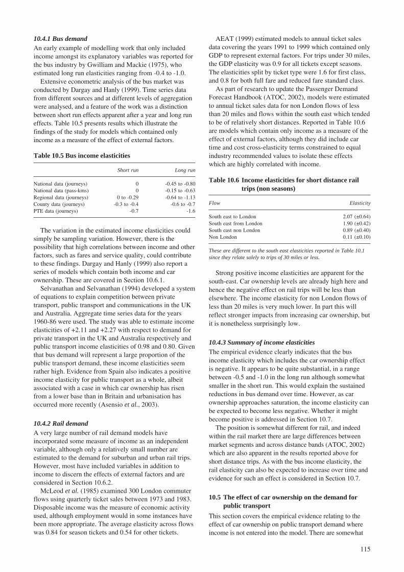
115

10.4.1 Bus demandAn early example of modelling work that only includedincome amongst its explanatory variables was reported forthe bus industry by Gwilliam and Mackie (1975), whoestimated long run elasticities ranging from -0.4 to -1.0.

Extensive econometric analysis of the bus market wasconducted by Dargay and Hanly (1999). Time series datafrom different sources and at different levels of aggregationwere analysed, and a feature of the work was a distinctionbetween short run effects apparent after a year and long runeffects. Table 10.5 presents results which illustrate thefindings of the study for models which contained onlyincome as a measure of the effect of external factors.

AEAT (1999) estimated models to annual ticket salesdata covering the years 1991 to 1999 which contained onlyGDP to represent external factors. For trips under 30 miles,the GDP elasticity was 0.9 for all tickets except seasons.The elasticities split by ticket type were 1.6 for first class,and 0.8 for both full fare and reduced fare standard class.

As part of research to update the Passenger DemandForecast Handbook (ATOC, 2002), models were estimatedto annual ticket sales data for non London flows of lessthan 20 miles and flows within the south east which tendedto be of relatively short distances. Reported in Table 10.6are models which contain only income as a measure of theeffect of external factors, although they did include cartime and cost cross-elasticity terms constrained to equalindustry recommended values to isolate these effectswhich are highly correlated with income.

Table 10.5 Bus income elasticities

Short run Long run

National data (journeys) 0 -0.45 to -0.80National data (pass-kms) 0 -0.15 to -0.63Regional data (journeys) 0 to -0.29 -0.64 to -1.13County data (journeys) -0.3 to -0.4 -0.6 to -0.7PTE data (journeys) -0.7 -1.6

Table 10.6 Income elasticities for short distance railtrips (non seasons)

Flow Elasticity

South east to London 2.07 (±0.64)South east from London 1.90 (±0.42)South east non London 0.89 (±0.40)Non London 0.11 (±0.10)

These are different to the south east elasticities reported in Table 10.1since they relate solely to trips of 30 miles or less.

The variation in the estimated income elasticities couldsimply be sampling variation. However, there is thepossibility that high correlations between income and otherfactors, such as fares and service quality, could contributeto these findings. Dargay and Hanly (1999) also report aseries of models which contain both income and carownership. These are covered in Section 10.6.1.

Selvanathan and Selvanathan (1994) developed a systemof equations to explain competition between privatetransport, public transport and communications in the UKand Australia. Aggregate time series data for the years1960-86 were used. The study was able to estimate incomeelasticities of +2.11 and +2.27 with respect to demand forprivate transport in the UK and Australia respectively andpublic transport income elasticities of 0.98 and 0.80. Giventhat bus demand will represent a large proportion of thepublic transport demand, these income elasticities seemrather high. Evidence from Spain also indicates a positiveincome elasticity for public transport as a whole, albeitassociated with a case in which car ownership has risenfrom a lower base than in Britain and urbanisation hasoccurred more recently (Asensio et al., 2003).

10.4.2 Rail demandA very large number of rail demand models haveincorporated some measure of income as an independentvariable, although only a relatively small number areestimated to the demand for suburban and urban rail trips.However, most have included variables in addition toincome to discern the effects of external factors and areconsidered in Section 10.6.2.

McLeod et al. (1985) examined 300 London commuterflows using quarterly ticket sales between 1973 and 1983.Disposable income was the measure of economic activityused, although employment would in some instances havebeen more appropriate. The average elasticity across flowswas 0.84 for season tickets and 0.54 for other tickets.

Strong positive income elasticities are apparent for thesouth-east. Car ownership levels are already high here andhence the negative effect on rail trips will be less thanelsewhere. The income elasticity for non London flows ofless than 20 miles is very much lower. In part this willreflect stronger impacts from increasing car ownership, butit is nonetheless surprisingly low.

10.4.3 Summary of income elasticitiesThe empirical evidence clearly indicates that the busincome elasticity which includes the car ownership effectis negative. It appears to be quite substantial, in a rangebetween -0.5 and -1.0 in the long run although somewhatsmaller in the short run. This would explain the sustainedreductions in bus demand over time. However, as carownership approaches saturation, the income elasticity canbe expected to become less negative. Whether it mightbecome positive is addressed in Section 10.7.

The position is somewhat different for rail, and indeedwithin the rail market there are large differences betweenmarket segments and across distance bands (ATOC, 2002)which are also apparent in the results reported above forshort distance trips. As with the bus income elasticity, therail elasticity can also be expected to increase over time andevidence for such an effect is considered in Section 10.7.

10.5 The effect of car ownership on the demand forpublic transport

This section covers the empirical evidence relating to theeffect of car ownership on public transport demand whereincome is not entered into the model. There are somewhat

116

fewer instances where car ownership is the sole variablerepresenting external factors. From an econometricstandpoint, this is as it should be since car ownership is notan exogenous variable and therefore it is more appropriateto use income as an independent variable in standardmultiple regression models or else use a statistical procedurewhich accounts for car ownership’s endogeneity.

10.5.1 Bus demandWe are not aware of studies of urban bus travel where thevolume of demand has been related solely to caravailability as a measure of external effects.Notwithstanding this, urban mode choice models, of whichvery many have been estimated, can be used to determinethe effect of car ownership on bus demand. This is becausethe choice set for those without a car contains just thepublic transport alternatives but is expanded to include carwhen one becomes available.

10.5.2 Rail demandMost rail demand models which contain car ownershipeffects relate to inter-urban travel (Fowkes et al., 1985;Rickard et al., 1986; Wardman, 1996) and hence arebeyond the scope of this report.

Wardman and Dunkerley (1999) specified a modelbased on NTS data which related rail trip rates per personto, amongst other things, whether there was no car in thehousehold. The data did not distinguish between long andshort distance trips and was based solely on leisure trips.The data were grouped into various socio-economiccategories, relating to gender, age group, socio-economicgroup, whether a car was owned and household type. Triprates were calculated for each combination of the variouscategories whilst the average income level for thatcategory was also obtained. The correlation betweenaverage income within a category and whether those in thecategory had a car or not was less than 0.3. The form ofthe model estimated was:

i i ji

NCH X

jj

V e Zβ λ

γµ+

=∑

∏

where V is the volume of rail trips per person in aparticular category, NCH is a dummy variable denotingwhether there was no car in the household, the X

i are

dummy variables relating to the other socio-economiccategories, and the Z

j are the average levels within each

category of continuous variables such as income and walktime to the station. Given average income levels variedlittle across categories, its effect was insignificant andhence the model contained only car ownership as ameasure of external effects.

In the above specification, the exponential of β denotesthe proportionate effect on rail trip rates per person of nothaving a car in the household. The parameter estimated tothe NTS data was 0.937 (±0.3). This indicates that, forconstant income, those without a car in the householdmade around 2½ times more rail trips13.

Studies by TCI (1989), Harris research Centre (1987)and Southgate and Associates (1986) demonstrate that carownership increases the choice of travel modes availableand increases the elasticities of rail service quality andprice. What is also clear is that an increase in competitionleads to higher rail demand elasticities, although the size ofthese changes depends upon journey purpose and the typeof competition.

10.5.3 Summary of car ownership elasticitiesFew studies have concentrated solely on car ownership as apredictor of the effects of external factors on public transportdemand. What evidence there is indicates that, as expected,the impact is negative. This is further illustrated by Table10.7. It shows that, on average in Great Britain, a person in acar owning household is likely to make considerably fewertrips by both bus (66% less) and rail (25% less)14 per weekthan a person in a non-car owning household.

The dearth of evidence of car ownership effects alone isperhaps surprising. The very many urban mode choicemodels in Great Britain rarely contain income as anexplanatory variable but they do indicate the effect of carownership through its impact on the set of alternativesbetween which the forecasting models allow individuals tochoose. In addition, census data are readily accessible at aspatially disaggregated level and contains figures relatingto household car ownership and to mode shares for thejourney to work. It would be a straightforward matter toexamine how modal shares vary with car ownership levels.

Whilst car ownership will have a negative impact uponthe demand for public transport the size of this impact doesdiffer from country to country. Table 10.8 shows the

Table 10.7 Journeys and kilometres per person a week according to household vehicle availability 1991/93in Great Britain

No Bicycles Motorcycle 1 2 3 or All Travel mode vehicles only /moped car cars more cars households

Journeys per personBus 3.3 3.0 2.1 1.1 0.7 0.5 1.5Rail 0.4 0.5 0.2 0.3 0.3 0.3 0.3

Kilometres per personBus 26.7 23.6 15.7 14.1 10.1 8.8 15.5Rail 11.7 14.7 10.4 12.1 11.3 13.2 12.0

Number of households 2,631(25.3%) 623(6.0%) 47(0.5%) 4,565(43.8%) 2,068(19.9%) 401(3.8%) 10,413(100%)

Source: Potter et al. (1997).

117

reported for Great Britain as a whole, with short and long runcar ownership elasticities of -1.04 and -1.43. Separate modelswere estimated for London, the Metropolitan areas, the non-Metropolitan areas, Wales and Scotland and the GDP and carownership elasticities are reported in Table 10.9.

Table 10.8 Car ownership and modal share in theEU (1999)

PublicCar transport

No of cars GDP per modal split modal splitper 1000 head in PPP (pkm in % (pkm in %

Country inhabitants (EU=100) for 1999) for 1999)

Belgium 450 (6) 111 (5) 81.8 17.1Denmark 341 (13) 118 (2) 79.4 19.8Germany 515 (3) 107 (7) 81.4 16.9Greece 275 (15) 67 (15) 66.7 21.9Spain 424 (8) 82 (13) 78.6 17.9France 465 (5) 101 (10) 84.3 14.2Ireland 346 (12) 112 (3) 80.3 18.9Italy 544 (2) 99 (12) 76.6 15.9Luxembourg 610 (1) 180 (1) 79.0 19.2Netherlands 398 (11) 112 (3) 81.5 16.6Austria 494 (4) 111 (5) 73.1 25.2Portugal 330 (14) 75 (14) 78.1 15.6Finland 407 (10) 103 (8) 81.6 17.0Sweden 440 (7) 101 (10) 80.2 18.6United Kingdom 414 (9) 102 (9) 86.8 12.5EU 15 460 100 81.0 15.9

Source: Statistical data – Eurostat (2001)

Table 10.9 Bus GDP and car ownership elasticitiesby area

NonMetro metro

London -politan -politan Wales Scotland

GDP 0.19 0.41 0.43 0.29 0.39(±0.08) (±0.14) (±0.16) (±0.23) (±0.17)

Car ownership -0.70 -1.04 -1.23 -2.01 -1.35(±0.48) (±0.23) (±0.27) (±0.41) (±0.30)

Table 10.10 Bus income and car ownership elasticities

Bus pass-kms Bus journeys

Car ownership short run 0 0Car ownership long run -0.73 -0.64Income short run 0.14 0.38Income long run 0.07 -0.26

relationship between car ownership and modal share in EUmember states for 1999. It can be seen that the UK has onaverage 414 cars per thousand inhabitants and a publictransport modal split of 12.5%. In comparisonLuxembourg has 47% more cars per thousand inhabitantsbut a public transport modal split of 19.2%. The lowestlevel of car ownership can be seen in Greece with 275 carsper thousand inhabitants, yet the highest share of publictransport is in Austria (25.2%) that has a car ownershiplevel of 494 cars per thousand inhabitants.

The figures in Table 10.8 help illustrate that, whilst carownership has a strong influence on the demand for publictransport, there are other direct and indirect influences atwork. These include:

� The cost of purchasing and operating a car, such as fuel,taxes and insurance.

� The cost of public transport, such as whether it issubsidised and whether the operators are efficient.

� Levels of congestion, for example, capital citiescompared to medium sized cities.

� Land use and social issues.

10.6 Joint effects of income and car ownership on thedemand for public transport

In this section, we consider models which have includedboth income and car ownership, or at least some proxy forthe latter, to explain variations in rail and bus demand.Whilst there are few studies which consider car ownershipin isolation, there are a number of studies which include italongside income.

10.6.1 Bus demandClark (1997) reported a number of demand elasticitiesestimated to aggregate time series data. Short and long runGDP per head bus demand elasticities of 0.33 and 0.45 are

The variation apparent across routes will no doubt havebeen influenced by the sampling distribution, since theelasticities are not very precisely estimated, but there areno clear symptoms of the expected collinearity problems.

A study by Fairhurst and Edwards (1996) estimatedregional UK bus trips per head using aggregate time seriesdata from 1970-94. The model for non-London flowsdemonstrated the multi-collinearity problems that can arisewhen both income (in this case consumer spending) andcar ownership are used in the same model. The modelproduced estimates that were intuitive in sign andmagnitude (+0.17 and -0.58 respectively) but, however,both were insignificant.

Dargay and Hanly (1999) estimated a structural modelof bus and car use to national time series data. Fourequations were specified, representing bus passengerkilometres, bus journeys, car ownership and car passengerkilometres. Independent variables included car ownership,bus fare, income and motoring costs. The income and carownership elasticities are reported in Table 10.10.

Although there is the issue of high correlation betweencar ownership and income, there is some evidence for anegative income effect in contrast to established thinking.This finding is apparent in another study considered below.

The National Travel Survey (NTS) provides a wealth ofinformation on travel behaviour at the individual andhousehold level and trends in it over time. Whilst its abilityto represent the fare and service quality characteristics ofdifferent modes is poor, it is able to examine the impact ofa wide range of socio-economic and demographicvariables including income and car ownership which are ofparticular interest here.

118

Another desirable feature of this type of data is that thedegree of correlation between the relevant measures ofincome and car ownership at the household or individuallevel is not high15. At the aggregate level, which coversmost of the studies we have dealt with in this chapter,income is represented by GDP and car ownership isrepresented by the proportion of households who havevarious numbers of car or the number of cars per capita.The degree of correlation between these aggregatestatistics is very high. In contrast, NTS data allows analysisto be conducted at the level of the individual. The relevantincome measure is therefore household or individualincome and the number of cars per household or whetherthe individual has a car. Whilst it is true that those withhigher incomes have a greater probability of having a car,the degree of correlation between household income andhousehold car ownership is not a cause for concern whenthe analysis is conducted at this level of detail. Forexample, the correlation between GDP and the number ofcars per household between 1985 and 1997 is 0.70. Thecorrelations in the NTS data for the same period betweenhousehold income and whether the household has one caror two or more cars are -0.09 and 0.36 respectively.

Wardman and Preston (2001) report mode choice andcar availability models which allow the estimation of theimpact of income on the demand for rail and bus for thejourney to work. The mode choice model is of themultinomial form and contains car driver, passenger, busand rail and covers the years 1985 through to 1997. It hasbeen recalibrated to remove time trend terms so that allinter-temporal effects are discerned by income andchanges in the choice set. The choice set of whether a caris available for the journey to work is analysed using alogit model for the same years and again the time trendterms in the model reported by Wardman and Preston havebeen removed. The estimated models are reported in theAppendix to Chapter 10.

The models have been used to forecast the effect ofchanges in income on mode share for the journey to work.This includes the indirect effect of income on caravailability, which varies those who can choose car, andthe direct effect of income on mode choice. For a 2%increase in income, which roughly corresponds withannual income growth, the overall income elasticity was–1.08 for bus. This figure does not vary greatly with thesize of the income variation.

Analysis of the same NTS data between 1985 and 1997for business and leisure trips involved the development oftwo models. The first model determines whether anindividual made a bus trip in the survey period and thesecond model analyses variations in the number of bus tripsby those who make them. The full models are reported inthe Appendix to Section 10. A logit model is used to explainwhether an individual makes any bus trips as a function ofvariables such as income, whether the household has one ormore than one car, employment status, age, gender, regionand a number of other socio-economic and demographicfactors. For those who do make bus trips, a further model isestimated to explain variations across individuals and overtime as a function of the same range of socio-economic anddemographic variables.

In the models of whether bus trips are made or not, itwas found that the income effect was positive for businessbut was absent for leisure trips whilst the coefficientsrelating to whether the household had one or more thanone car both indicated a negative effect with the latterlarger than the former.

In the model based on explaining the number of bus tripsgiven that at least one is made, the income elasticity waseffectively zero for business but actually negative albeitsmall (-0.04) for leisure trips. As income increases, theremay be a greater tendency to use taxis, although trends insocial attitudes may be at work here. Whether the householdhad one car reduced the number of bus leisure trips by 24%whilst more than one car in the household reduced thenumber of trips by 29%. For bus business trips, there wereno effects apparent from household car ownership.

Income will therefore have a direct effect on the numberof bus trips and also indirectly through car ownership.Table 10.11 reports income elasticities for 2%, 5% and 10%increases in income for the final year in the data sets analysedof 1997. Increases in the number of households with one carand two or more cars solely as a result of income growth wasforecast using the Department for Transport’s car ownershipforecasting model (Whelan, 2001).

Table 10.11 Bus income elasticities (including carownership effects)

Income Business Leisure

+2% 0.49 -0.33+5% 0.50 -0.33+10% 0.51 -0.33

The overall income elasticity for business trips ispositive and quite strong, although this is a relativelyunimportant market segment. For leisure trips, the overallelasticity is negative, in line with the income elasticitiesestimated when it is the only variable to represent externaleffects. The measure of income used is household income.Whilst a better measure would be a variable relating tonational income, which reflects the level of economicactivity, variation in household income over time will tendto correlate with variation in national income. Section 10.7considers how the income elasticity will vary over time ascar ownership levels more closely approach saturation.

10.6.2 Rail demandWithin the rail industry, there has been a long tradition ofspecifying the effects of external factors in terms of GDPand a time trend. The latter term represents the effects of arange of external factors, but is generally taken to bedominated by increasing car ownership and hence isexpected to be negative.

Glaister (1983) examined rail commuting into London.The earnings elasticity varied between 0.56 and 1.69depending upon route and model formulation, with a smallpositive time trend and also small unemploymentelasticities of the expected signs for the origin anddestination location.

119

Palomo (1996) estimated models to time series datarelating to trips on Network South East services. These aredominated by trips to London, with commuting trips andshorter distance trips forming a large proportion. The GDPelasticity was estimated to be 1.1 with a negative timetrend of -1.7% per annum. In similar analysis, Clark(1997) estimated the GDP elasticity to be 0.62 and the carownership elasticity to be 0.32 for these flows. Thepositive car ownership effect is presumably due to strongcorrelation with income.

TCI-OR (1997) estimated models to rail tickets sales datarelating to the periods quarter 2 1987 through to quarter 41995. Separate models were estimated to flows less than 25miles and the results are presented in Table 10.12.

the existing rail market share. Nonetheless, the figuresexceed one by some considerable amount, and theemployment elasticity may also be discerning othereffects, such as trends in car journey times and costs. Inthis context, there will be little negative impact due to carownership. This along with rail demand growth due toincreased road congestion presumably accounts for thepositive trend.

There is also a suspicion of correlation problems in theresults for full fare, with a correlation between the timetrend and GDP elasticity estimates of -0.42. However,some of the variation could simply be due to samplingdistribution. The stark difference between the results forfull fare and reduced tickets suggests that there might havebeen switching between ticket types which has not beenadequately accounted for.

As part of a study to develop a rail industry forecastingframework, models were estimated to time series ticketsales data for trips in the south east to London (SteerDavies Gleave, 1999b). Separate models were estimatedfor season tickets, full fare tickets and reduced tickets fortrips less than 35 miles. For season tickets, an employmentelasticity of 1.32 was estimated along with a quarterlynegative time trend of -0.59%. For full fare tickets, theGDP elasticity was 2.57 with a trend of 0.12% per quarterwhilst for reduced tickets the corresponding values were1.05 and 0.35% per quarter. The large negative time trendfor season tickets is a cause for concern, whilst the GDPelasticity for full fare tickets seems large, particularlygiven the positive trend associated with these tickets.Switching between ticket types was not explicitly allowedfor and could well have influenced these results.

The problem of correlation between economic variablesand the time trend or other measures such as car ownershipis evident in many studies of longer distance travel(ATOC, 2002). A ‘solution’ in some studies is to constrainthe time trend. For example, in analysis of ticket sales datato determine the impact of service disruptions due to themajor redevelopment of Leeds station, Wardman et al.(2001b) constrained the time trend in a model of suburbanrail trips to equal -2% per annum which was the thenrecommended figure in the Handbook. The resulting GDPelasticity was 1.66 for all flows except 4.44 for trips toLeeds. The high value for the latter is the result of usingnational figures which dramatically underestimated thegrowth in the Leeds economy in the period in question. Inaddition, increases in fuel costs and car journey times werenot accounted for and can have been expected to inflatethe GDP elasticity.

Subsequent developments in forecasting in the railindustry have placed more emphasis on car ownershiplevels. The rail industry forecasting framework (SteerDavies Gleave, 1999b) includes a car ownership elasticityfor leisure trips and also for business trips outside thesouth east, whilst retaining a time trend in some marketsegments. In contrast, the most recent version of thePassenger Demand Forecasting Handbook (ATOC, 2002)includes a non-car ownership term and removes the timetrend altogether. The recommended forecasting frameworkin the Handbook for what are termed external factors is:

Table 10.12 GDP elasticity and time trend estimates(journeys < 25 miles)

Seasons Other

Flow GDP Trend GDP Trend

Intercity non London 0.1 -1.3% -0.32 -1.3%South east London 3.5 -7.6% 1.94 -2.1%South east non London 2.2 -4.3% 1.21 -2.8%Regional 1.8 -3.6% 0.47 3.1%

Table 10.13 Economic activity and trend parametersfor London and south east rail flows

Ticket type South North NorthVariable All South West West North East

Season ticketsEmployment 2.0 1.3 0.9 2.6 1.7 1.9Trend 1.4% 1.3% 1.6% 2.4% 1.2% 1.3%

Full fare ticketsGDP 1.9 0.7 2.0 2.2 3.4 1.6Trend -3.2% -3.7% -3.4% -2.4% -4.7% -2.3%

Reduced ticketsSpending 1.9 1.8 1.9 2.4 1.9 1.7Trend 2.2% 1.1% 2.8% 2.6% 2.2% 2.4%

Whilst we might expect variation in these parametersacross routes, the results are consistent with the presence ofmulticollinearity. Thus larger GDP elasticities will beassociated with more negative time trends, and this pattern isapparent in the results. This study also examined a lagstructure but found no strong support for such a specification.

Similar findings are apparent in the study of Centre forEconomics and Business Research (1998) where thespecification of rail demand models for trips in the south eastinto London included a measure of economic activity and atime trend. Models were developed to time series CAPRI datafor season tickets, standard and first class tickets, and reducedfare tickets, for the period 1987-1996, and the key findingsfor various corridors are reported in Table 10.13.

As expected, given the highly congested roads that facecommuters into London, the employment elasticityexceeds one since the proportion of additional tripsgenerated by employment growth that use rail will exceed

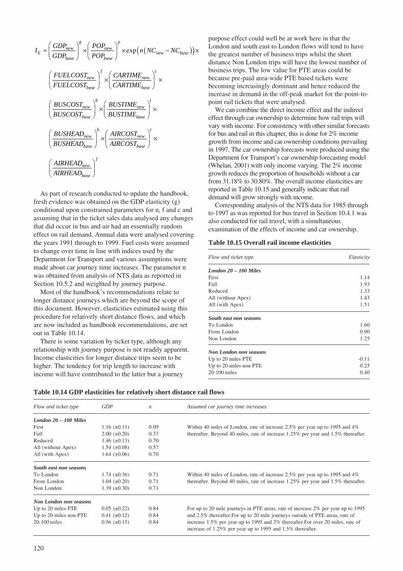
120

( )( )expg p

new newE new base

base base

GDP POPI n NC NC

GDP POP

⎛ ⎞ ⎛ ⎞= × × − ×⎜ ⎟ ⎜ ⎟⎝ ⎠ ⎝ ⎠

f cnew new

base base

FUELCOST CARTIME

FUELCOST CARTIME

⎛ ⎞ ⎛ ⎞× ×⎜ ⎟ ⎜ ⎟

⎝ ⎠ ⎝ ⎠

b tnew new

base base

BUSCOST BUSTIME

BUSCOST BUSTIME

⎛ ⎞ ⎛ ⎞× ×⎜ ⎟ ⎜ ⎟

⎝ ⎠ ⎝ ⎠

b rnew new

base base

BUSHEAD AIRCOST

BUSHEAD AIRCOST

⎛ ⎞ ⎛ ⎞× ×⎜ ⎟ ⎜ ⎟

⎝ ⎠ ⎝ ⎠

fnew

base

AIRHEAD

AIRHEAD

⎛ ⎞⎜ ⎟⎝ ⎠

As part of research conducted to update the handbook,fresh evidence was obtained on the GDP elasticity (g)conditional upon constrained parameters for n, f and c andassuming that in the ticket sales data analysed any changesthat did occur in bus and air had an essentially randomeffect on rail demand. Annual data were analysed coveringthe years 1991 through to 1999. Fuel costs were assumedto change over time in line with indices used by theDepartment for Transport and various assumptions weremade about car journey time increases. The parameter nwas obtained from analysis of NTS data as reported inSection 10.5.2 and weighted by journey purpose.

Most of the handbook’s recommendations relate tolonger distance journeys which are beyond the scope ofthis document. However, elasticities estimated using thisprocedure for relatively short distance flows, and whichare now included as handbook recommendations, are setout in Table 10.14.

There is some variation by ticket type, although anyrelationship with journey purpose is not readily apparent.Income elasticities for longer distance trips seem to behigher. The tendency for trip length to increase withincome will have contributed to the latter but a journey

purpose effect could well be at work here in that theLondon and south east to London flows will tend to havethe greatest number of business trips whilst the shortdistance Non London trips will have the lowest number ofbusiness trips. The low value for PTE areas could bebecause pre-paid area-wide PTE based tickets werebecoming increasingly dominant and hence reduced theincrease in demand in the off-peak market for the point-to-point rail tickets that were analysed.

We can combine the direct income effect and the indirecteffect through car ownership to determine how rail trips willvary with income. For consistency with other similar forecastsfor bus and rail in this chapter, this is done for 2% incomegrowth from income and car ownership conditions prevailingin 1997. The car ownership forecasts were produced using theDepartment for Transport’s car ownership forecasting model(Whelan, 2001) with only income varying. The 2% incomegrowth reduces the proportion of households without a carfrom 31.18% to 30.80%. The overall income elasticities arereported in Table 10.15 and generally indicate that raildemand will grow strongly with income.

Corresponding analysis of the NTS data for 1985 throughto 1997 as was reported for bus travel in Section 10.4.1 wasalso conducted for rail travel, with a simultaneousexamination of the effects of income and car ownership.

Table 10.14 GDP elasticities for relatively short distance rail flows

Flow and ticket type GDP n Assumed car journey time increases

London 20 – 100 MilesFirst 1.16 (±0.11) 0.09 Within 40 miles of London, rate of increase 2.5% per year up to 1995 and 4%Full 2.00 (±0.20) 0.37 thereafter. Beyond 40 miles, rate of increase 1.25% per year and 1.5% thereafter.Reduced 1.46 (±0.13) 0.70All (without Apex) 1.54 (±0.08) 0.57All (with Apex) 1.64 (±0.06) 0.70

South east non seasonsTo London 1.74 (±0.36) 0.71 Within 40 miles of London, rate of increase 2.5% per year up to 1995 and 4%From London 1.04 (±0.20) 0.71 thereafter. Beyond 40 miles, rate of increase 1.25% per year and 1.5% thereafter.Non London 1.39 (±0.30) 0.71

Non London non seasonsUp to 20 miles PTE 0.05 (±0.22) 0.84 For up to 20 mile journeys in PTE areas, rate of increase 2% per year up to 1995Up to 20 miles non PTE 0.41 (±0.12) 0.84 and 2.5% thereafter.For up to 20 mile journeys outside of PTE areas, rate of20-100 miles 0.56 (±0.15) 0.84 increase 1.5% per year up to 1995 and 2% thereafter.For over 20 miles, rate of

increase of 1.25% per year up to 1995 and 1.5% thereafter.

Table 10.15 Overall rail income elasticities

Flow and ticket type Elasticity

London 20 – 100 MilesFirst 1.14Full 1.93Reduced 1.33All (without Apex) 1.43All (with Apex) 1.51

South east non seasonsTo London 1.60From London 0.90Non London 1.25

Non London non seasonsUp to 20 miles PTE -0.11Up to 20 miles non PTE 0.2520-100 miles 0.40

121

For commuting trips, the combined car availability andmode choice model implied an income elasticity for rail in1997 of 0.34. For business and leisure trips, separatemodels were estimated to explain whether a rail trip wasmade in the survey period and to explain variations in tripsby those who made them. No distinction was madebetween urban and inter-urban trips. Full details of themodels are reported in Appendix 6.3.

For both business and leisure trips, the probability ofmaking a trip increases with income but falls as car ownershipper household increases. With respect to variations in thenumber of trips by those who make rail trips, the incomeelasticity is positive for leisure trips but zero for business trips.The effects of car ownership on the number of rail trips isslight. For business trips, no significant effect was obtainedwhilst for leisure trips the presence of one car per householdreduced rail trips by 9% and two or more cars per householdreduced rail trips by 11%.

The overall income elasticities, combining the directeffect of income and its indirect effect through carownership, were obtained using the same procedure as forbus reported in Section 10.6.1 and again relate to 1997.The elasticities are given in Table 10.16 and again wouldimply healthy growth in rail demand with income growth.

income and car ownership. With regard to bus travel demand,Dargay and Hanly (1999) state that, ‘It should be stressed,however, that the negative income elasticity pertains to aperiod of rising car ownership and use. As private motoringreaches saturation, which it must do eventually, or is limitedby political means, it is likely that income’s negative effect onbus patronage will become smaller, and possibly becomepositive’. For the same reasons, rail income elasticities can beexpected to become larger.

To address the extent to which the income elasticitiesmight increase, we have repeated the forecasting exercisesreported in Tables 10.11 and 10.16 based on NTS models.This has been done for 2% income growth from theincome and car ownership situations for 2005, 2015 and2025. It is assumed that income grows by 2% per annum.The car ownership forecasts for zero (P0), one (P1), two(P2) and three plus cars (P3+) per household, again basedon the Department for Transport’s official model, assumeonly that income changes over time. The forecastsproduced by this model are given in Table 10.17.

Table 10.16 Rail income elasticities (including carownership effects)

Income Business Leisure

+2% 0.72 0.41+5% 0.74 0.42+10% 0.76 0.43

Table 10.17 Car ownership forecasts used in calculatingincome elasticities

Year P0

P1

P2

P3+

1997 0.3118 0.4378 0.2059 0.0446+2% 0.3080 0.4380 0.2085 0.0455

2005 0.2828 0.4382 0.2273 0.0518+2% 0.2802 0.4380 0.2293 0.0525

2015 0.2496 0.4342 0.2542 0.0619+2% 0.2468 0.4336 0.2567 0.0629

2025 0.2215 0.4270 0.2789 0.0726+2% 0.2187 0.4262 0.2813 0.0738

Table 10.18 Overall bus and rail elasticities based onanalysis of NTS data

Commuting Business Leisure

Bus Train Bus Train Bus Train

1997 -1.08 0.34 0.49 0.72 -0.33 0.422005 -1.27 0.40 0.66 0.89 -0.30 0.522015 -1.60 0.49 0.80 1.09 -0.29 0.612025 -2.08 0.53 1.00 1.34 -0.28 0.75

10.6.3 Summary of combined income and car ownershipeffects

In studies based on the volume of demand, there is strongcorrelation between income and car ownership whichmeans that it is difficult to disentangle the separate effectsof each. In some instances, it has even resulted incoefficients of wrong sign. Various studies have attemptedto overcome this problem using outside evidence andconstrained estimates whilst analysis of trip patterns at theindividual level, as is possible with NTS data, does notface serious correlation problems.

There is some evidence to suggest that variations in thedemand for bus purely as a result of income growth arenegative, but in any event the overall effect after theintroduction of car ownership is negative. Although carownership has a negative impact on rail demand, it is lessthan for bus and, although there are quite large variationsacross studies and type of route, the overall effect ofincome on rail demand is quite strongly positive.

10.7 Posible variations in income elasticity over time

It is often argued that multicollinearity is not a particularproblem for forecasting provided that the degree ofcorrelation is maintained over the forecasting period.However, this is unlikely to be the case in the context of

The overall income elasticities for 2% income growth ineach of several future years and based on models whichhave analysed NTS data are reported in Table 10.18. Themodels project significant increases in the overall railincome elasticities over time. For bus, the findings aremixed. In the business market, there is growth in theelasticity but this is a minor market segment, yet in theleisure market there is hardly any variation in the overallincome elasticity over time and by no means could it beconcluded that the overall income elasticity would becomepositive. The increasing negative elasticity in the buscommuting market is a result of the logit model’s propertythat the absolute value of an elasticity will increase as busmarket share falls over time and as income grows over time.

122

10.8 Conclusions and recommendations

10.8.1 ConclusionsThe main focus of this chapter has been to disentangle theeffects of income and car ownership upon the demand forpublic transport. In so doing a number of other topics havebeen covered.

Examination of the effect of income on travelexpenditure and distance travelled has shown that thepercentage of overall household expenditure spent ontransport and travel has been rising steadily in GreatBritain since 1981. There is clear evidence that trip lengthsare increasing with income for all modes and all trippurposes, though the effects are not particularly strong. Ingeneral, the elasticities lie in the range 0.09 to 0.21, withnoticeably stronger growth for car commuting, businesstrips by rail and business trips by bus.

The empirical evidence of the of the effect of incomeand car ownership respectively on public transport demandclearly indicates that the bus income elasticity whichincludes the car ownership effect is negative, ranging from-0.5 to -1.0 in the long run. It was felt that has carownership approaches saturation, the income elasticity canbe expected to become less negative. Few studies haveconcentrated solely on car ownership as a predictor of theeffects of external factors on public transport demand.What evidence there is indicates that, as expected, theimpact is negative.

Regarding the joint effects of income and carownership on the demand for public transport, there issome evidence to suggest that variations in the demandfor bus purely as a result of income growth are negative,but in any event the overall effect after the introductionof car ownership is negative. Although car ownership hasa negative impact on rail demand, it is less than for busand, although there are quite large variations acrossstudies and types of route, the overall effect of income onrail demand is quite strongly positive.

An attempt was made to examine the possible variationsin income elasticity over time. The results from a number offorecasted models signify significant increases in the overallrail income elasticities over time. For bus the findings aremixed. In the business market, there is growth in theelasticity but this is a minor market segment. In the leisuremarket there is hardly any variation in the overall incomeelasticity over time and by no means can it be concludedthat the overall income elasticity will become positive.

10.8.2 RecommendationsThe analysis of NTS data indicates overall incomeelasticities for bus of -1.08 for commuting and -0.33 forleisure trips. Bearing in mind the balance betweencommuting and leisure trips, these figures are broadlyconsistent with Dargay and Hanly (1999) who estimatedlong run elasticities of:

� National -0.45 to -0.80.

� Regional -0.64 to -1.13.

� County -0.6 to -0.7.

We therefore recommend that the NTS figures can beused as long run elasticities, and also to provide adisaggregation by purpose and for changes in elasticitiesover time.

With regard to suburban rail, the ticket sales evidencecovers a large range, with values of 0.5 to 2.0representing London and 0.1 to 0.9 representingelsewhere. However, there are other confounding effectsapparent, such as switching between ticket types andincreasing road congestion.

The NTS evidence for rail indicates elasticities of 0.34for commuting, which is in addition to employmenteffects, 0.72 for business and 0.42 for leisure. Thesefigures can be taken as broadly consistent with the ticketsales evidence.

For rail, it is recommended that the NTS evidence isused. This also provides segmentations by purpose andallows for changes in the overall income elasticity overtime. In addition, a key driver of commuting trips isemployment.

Finally the NTS evidence on journey length and incomethere is clear evidence that trip lengths are increasing withincome, although the effects are not particularly strong. Ingeneral elasticities lie in the range of 0.09 to 0.21 but withnoticeably stronger growth for car commuting. Theseelasticities are somewhat higher, between 0.11 to 0.35, ifvariables associated with income (employment status etc)are stripped out.

11 The relationship between land-useand public transport

11.1 Introduction

The relationship between land use and transport iscomplex and difficult to fully unravel. Both are part of adynamic system and interact at several different scaleswithin the urban environment – at the neighbourhoodlevel, at the city district level through to the urban region(i.e. the urban area and the hinterland which it services)and beyond. Land-use patterns are also a difficult conceptto quantify and are a result of the interaction of manyhistorical forces. Generally, land use patterns are describedusing a number of different characteristics such as thedistance from the urban centre, settlement size, mix of landuses, the level of provision of local facilities, the density ofdevelopment, proximity to transport networks, settlementshape and urban form. Each of these measures is onlyindicative of one aspect of land use. Boarnet and Crane(2001) found that the measured relationship between landuse and transport was very sensitive to the choice ofempirical methodology. Different land-use characteristicsare often associated with each other. For example,historically areas of high population densities tended to belocated near the city centres in areas with good publictransport provision. However, just because this associationhas existed in the past, it does not mean that with thecreation of high-density residential areas in the future thatgood public transport provision will follow.

123

The relationship between land-use and transport iscomplicated still further by the close association of bothelements with a number of socio-economic factors such ascar ownership and income, which themselves areinterrelated. Different land-use characteristics are oftenassociated with different socio-economic factors, andsocio-economic factors also affect travel patterns (Stead et al.,2001). Variations in socio-economic characteristics add tothe complexity of the problem, making it difficult toestablish the precise relationships between public transportdemand and land-use patterns.

The chapter begins by considering the effect of land-usepatterns in general on transport demand and the effect ofdifferent planning policies on travel patterns. It then goeson to explore the effect of transport infrastructure andprovision on economic growth and development patterns,which will in turn affect the demand for public transport,before briefly addressing how transport policy can be usedto guide planning policy.

11.2 The effects of land-use on public transport demand

Land-use patterns and built form can influence transportdemand in the following ways:

Interspersion of activities � trip lengths and trip frequency.

Shape of the urban area � trip lengths.

Density � trip lengths and trip frequency.

Clustering of trip ends � public transport.

Settlement size � trip lengths, public transport.

(Adapted from Owens,1986)

All these elements are interrelated, and the relationshipbetween them and transport will depend on the definitionof the variable used to measure each element.

The effect of land use on travel varies by trip purpose.As with fares, the effect of land use change on a particularjourney will depend on the degree to which the journeystart/end time, mode, route and destination can bechanged, whether the journey is essential or non-essentialand the degree to which it is (and can be) linked with othertrips. Maat (1999) suggests that land-use has the biggesteffect on commuting trips and local/convenience shoppingjourneys. Boarnet and Greenwald (2000) suggest for non-work trips land-use influences the distances travelledrather than the number of trips made.

11.2.1 DensityIt can be expected that the number of journeys made perperson by public transport will increase with density;whilst the average length of journeys will decrease withincreasing density. This is reflected in the results shown inTables 11.1 and 11.2. As can be seen both bus and rail useincrease with density. Walking also increases with density,whilst car use decreases. Van Diepen (2000) found similarresults in an analysis of 1995 travel survey data for theNetherlands.

The relationships between journey distance and densityseem to be weakening over time. ECOTEC (1993) alsofound some evidence that the relationship between densityand mode split has been weakening over time. This ispossibly due to decentralisation, with an increasing

Table 11.1a Distance travelled per person per week bymode and population density 1985/6

Density Distance travelled per person per week by modePersonsper All Localhectare modes Car bus Rail* Walk Other†

<1 206.3 159.3 5.2 8.9 4.0 28.81-5 190.5 146.7 7.7 9.1 4.9 21.95-15 176.2 131.7 8.6 12.3 5.3 18.215-30 152.6 105.4 9.6 10.2 6.6 20.630-50 143.2 100.4 9.9 10.8 6.4 15.5>50 129.2 79.9 11.9 15.2 6.7 15.4All areas‡ 159.6 113.8 9.3 11.3 5.9 19.1

* Includes long distance rail.

† Other refers to two-wheeled motor vehicles, taxis, domestic air travel,other public transport and other types of bus (school, hire, expressand works).

‡ Data excludes all trips less than 1.6km and only refer to the mainmode used for a trip.

Source: Based on ECOTEC (1993).

Table 11.1b Distance travelled per person per week bymode and population density 1999/2001

Density Distance travelled per person per week by modePersonsper All Localhectare modes Car bus Rail* Walk Bicycle Other†

<1 171.51 145.56 4.21 6.17 2.57 0.86 12.141-5 159.43 133.22 3.93 8.72 2.70 0.82 10.035-15 133.97 111.11 3.89 6.23 3.23 0.73 8.7815-30 124.19 96.57 4.41 9.42 3.21 0.79 9.7830-50 111.75 86.38 5.02 7.59 3.45 0.61 8.71>50 94.75 63.02 6.13 15.04 3.63 0.64 6.28All areas‡ 130.41 103.93 4.58 8.84 3.17 0.73 9.17

* Includes long distance rail, LT Underground and Light Rail.


‡ Data only refer to the main mode used for a trip.


number of businesses relocating away from the city core tosuburban and fringe locations.

ECOTEC (1993) found the following relationshipsbetween population density and travel patterns:

� Higher pop densities widen the range of opportunitiesfor the development of local contacts and activities,without the need to use motorised transport.

� Higher pop densities increase the scale of localexpenditure widening the range of services whichpotentially can be supported and therefore:

� Higher pop densities will tend to reduce averagedistances between place of residence and the places atwhich services/employment opportunities can beaccessed (provided that the higher population densitiesare accompanied by increases in commercial densities,for example Frank and Pivo (1994) showed that highemployment density, high population density and amixed land use pattern all help increase public transportuse for work and shopping trips.

124

� Increasing the density of population shortens the accessdistances to the public transport network and createsgreater numbers of personal movements along specificcorridors, thus improving the viability of public transport.

All of the above impacts of increased populationdensities assume that the areas of high population densityare within reasonable proximity to a range of services,facilities and public transport. In addition the benefits fromany increases in population can only be accrued if they areaccompanied by similar increases in commercial densities.However, these greater numbers of movements can alsocreate greater levels of congestion, which could slow downpublic transport movements, discouraging trips.

However, the relationships outlined above also suggestthat at high densities, shorter journey lengths could resultin an increase in non-motorised trips leading to a decreasein public transport. Indeed this was one of the findings ofthe ECOTEC report (ECOTEC, 1993). ECOTEC foundthat the number of journeys made on foot increased with

higher neighbourhood densities but unlike public transport,this relationship was unaffected by car ownership and theoccupational characteristics of the area.

A major problem when analysing the effect of densityon travel patterns is the high degree of association betweendensity, socio-economic characteristics (includingincome), public transport provision and prices, and carownership. For example, Fouchier (1997) found arelationship between car ownership and what he refers toas ‘net human density’ for the Paris region. Net humandensity or ‘urban intensity’ is defined as (population +employment)/urban hectares. Fouchier found that thecorrelation between ‘non-motorisation’ (the number ofhouseholds with no car) and density was stronger(R=+0.71) than the relationship between average carownership levels and density. Fouchier surmises that thisconfirms the theory that higher densities provide for thepossibility of not using a car. Unfortunately, Fouchier doesnot go on to relate density to levels of public transport use.

Breheny (1995a) suggests that social class and carownership are likely to explain additional variations in therelationship between density and public transport use.Breheny used journey to work data from the 1991 Census ofPopulation to compare public transport use with density forGreater London. The data refer to the main mode usually usedfor the journey to work, and the overall population density forurban areas16. Breheny found that public transport use (busand rail) for the journey to work was related to density (R2 =52%). The regression equation is given as:

%Bus/Rail = 19.2 + 0.337 Density

Including social class in the regression analysisincreased the R2 value to 56%:

%Bus/Rail = 29.2 + 0.269 Density - 0.244 Social Class

The inverse relationship between bus/rail use and socialclass indicates that the higher the percentage of householdsin social classes 1 and 2, the lower the level of commutingby public transport. Breheny repeated the analysis for aselection of counties in the rest of the south east (ROSE).In this case relationship between density and publictransport use was much weaker (R2 = 0.11). Similarly, hefound no clear relationship between public transport useand social class.

Newman and Kenworthy (1989)17 examined the linkbetween urban form and transport using data from 32world cities. They found strong correlations between urbanform and transport. Measures of public transport useexamined included public transport passenger km percapita, private car/public transport balance (% of totalpassenger kms on public transport), public transportpassenger trips per person and the proportion of publicworkers using public transport. Urban form variablesexamined included population and job densities across theurban area, in the CBD, and in inner and outer areas; aswell as the distribution of population and jobs between thedifferent areas. No significant correlations were foundbetween transport and CBD job density. Newman andKenworthy (1991) conclude from this that it would appearthat in order to lessen automobile dependence it is moreimportant to have higher residential densities mixed in

Table 11.2a Number of journeys per person per weekby mode and population density 1985/6

Density Journeys per person per week by modePersonsper All Localhectare modes Car bus Rail* Walk Other†

<1 13.59 9.72 0.55 0.11 1.40 1.811-5 14.81 10.28 1.04 0.23 1.78 1.485-15 14.69 10.10 1.28 0.25 1.87 1.1915-30 14.12 8.74 1.53 0.24 2.38 1.2430-50 13.97 8.38 1.77 0.37 2.33 1.12>50 12.99 6.68 2.21 0.63 2.47 1.00All areas‡ 13.98 8.75 1.52 0.33 2.14 1.25

* Includes long distance rail.


‡ Data exclude all trips less than 1.6km and only refer to the main modeused for a trip.

Source: Based on ECOTEC (1993).

Table 11.2b Number of journeys per person per weekby mode and population density 1999/2001

Density Journeys per person per week by modePersonsper All Localhectare modes Car bus Rail* Walk Bicycle Other†

<1 19.42 13.16 0.56 0.12 4.40 0.31 0.881-5 19.95 13.80 0.66 0.23 4.27 0.33 0.665-15 20.64 13.36 0.92 0.23 5.18 0.29 0.6615-30 19.90 12.26 1.13 0.36 5.14 0.35 0.6530-50 19.19 11.36 1.28 0.37 5.27 0.27 0.63>50 18.32 8.26 1.85 1.14 6.20 0.25 0.63All areas‡ 19.63 12.07 1.09 0.40 5.10 0.30 0.67

* Includes long distance rail, LT Underground and Light Rail.


‡ Data only refer to the main mode used for a trip.


125

with the employment activity. Residential density in theCBD does correlate strongly with transport patterns. Astudy of US cities by the Transit Cooperative ResearchProgram (TRCP, 1995 cited in Newman and Kenworthy,1999) confirmed the exponential relationship found byNewman and Kenworthy between density and publictransport ridership. The study estimated that elasticity forresidential density and ridership was 0.6.

Breheny and Gordon (1996), amongst others, makeseveral criticisms of the Newman and Kenworthy work.The key criticism concerns the degree of associationbetween density, public transport provision, prices, incomeand car ownership, which Newman and Kenworthy failedto account for in their analysis. Breheny and Gordon(1996) used regression analysis to combat the problem ofassociation and found that almost as high a value for R2

could be produced when density was excluded from theregression model as when it was included.

Cervero (1996) showed that the probability ofcommuting by public transport decreases if one lives in aneighbourhood with single-family detached dwellings andincreases in areas of attached housing. But, he found thatother variables such as an adequate public transport serviceand living near the city centre were more significant thanthe land-use pattern, and that increasing car ownership hada major impact. Similarly, Friedman et al. (1994) showthat public transport use is higher for all trip purposes intraditional neighbourhoods compared with suburban areas.

There is also a relationship between density and parkingprovision (Hall, 2001). In high density areas parkingprovision may be limited. If parking is in short supply,then residents may choose not to own a car. Also, they willbe less likely to use the car if other modes, such aswalking, can be substituted, due to the length of time itmay take to find a suitable parking space on their return.

A second complication is the measurement of densityitself. The relationship between density and public transportuse varies considerably depending on whether the density isaveraged across an estate, district or city region and the unitof measurement i.e. dwellings, buildings, or population. Forexample, Stead (2001) analysed the relationship betweentravel distance, land-use characteristics and socio-economiccharacteristics using a number of different data setsincluding the National Travel Survey. He found no evidenceof a link between travel distance and local authoritypopulation density. However, he did find a link betweenward level density and average travel distance, withresidents of low-density wards travelling longer distancesthan the residents of most other wards.

The location of the boundaries of the area across whichdensity is calculated is also important. For example, manylocal authority districts boundaries are not closely alignedwith urban areas. Some borough boundaries include a ruralarea as well as the main urban area as in the case of MiltonKeynes; other urban areas are under-bounded by the districtboundary, e.g. Reading. Under-bounding is likely to increasethe density value whilst over-bounding will reduce the densityvalue. In addition, density can vary considerably across adistrict and neighbourhood densities may be as important ascity densities in determining travel behaviour as these will

affect aspects such as the distances travelled to reach a busstop. Ecotec (1993) found that density at the local authoritylevel had a positive influence on the proportion of work-related travel undertaken by public transport and that thisrelationship also holds at the urban level.

11.2.2 Settlement sizeAnother element of built form that could influence transportis settlement size. Settlement size, in terms of population,affects the choice of facilities available to meet a particularactivity need and the extent to which higher order servicesand facilities are provided within the local urban area.Settlement size will also affect the distances that need to betravelled to reach particular services and facilities. This isalso dependent on the density of the settlement and its form.Finally, settlement size will affect the modes of transportthat can be supported by the urban area.

Public transport ridership tends to increase withincreasing settlement size (Table 11.3), as does the distancetravelled on public transport per person per annum (Table11.4). However, the mean trip distance tends to decreasewith increasing settlement size (Table 11.5).

ECOTEC (1993) found using 1985/6 National TravelSurvey data that population size was not related to travelbehaviour in a simple linear relationship. Whilst the distancetravelled per person per week by local bus was found todecrease with decreasing size, no obvious pattern was foundfor rail travel. These findings still hold true. Table 11.3shows that while the number of bus trips made per annumper head of population between 1999 and 2001 increaseswith increasing settlement size, the number of rail trips perhead of population shows no obvious trend. Average busjourney lengths tend to increase with decreasing settlementsize, but again with rail it is difficult to discern a trend(Table 11.5). Rail trips made by residents of London tend tobe considerably shorter than the average GB rail trip; whilstrail trips from rural areas tend to be considerably longer thanaverage. The balance between bus and rail travel is different

Table 11.3 Trips per person per year by mode in GreatBritain by area type, 1999/2001

Total number of trips per head

LocalWalk Car bus Rail* Other‡ Total

London Boroughs. 299 468 94 87 42 990

Metropolitan built-up areas. 264 591 94 8 38 995

Large urban areas, over 271 628 66 12 42 1019250k population.

Medium urban areas, over 268 658 47 12 44 102925 to 250k.

Small/medium urban areas, 261 714 38 10 45 106810 to 25k.

Small urban areas, 3 to 10k. 253 674 29 † 51 1007

Rural areas. 204 742 27 7 36 1016

All areas. 263 638 57 20 41 1019

* Includes long distance rail.† Sample size too small for reliable estimate.‡ Includes some rounding errors.

Source: Department for Transport (2002b).

126

for metropolitan areas compared with non-metropolitanareas (Tables 11.3-11.5).

Commuting by bus increases with increasing settlementsize (Table 11.6). Whilst school trips by bus show a morecomplex pattern, with a minimum of 25% for mediumsized urban areas (over 25k and under 250k). LocalEducation Authorities (LEAs) in Britain are obliged toprovide free travel for pupils above certain distances fromschool. In lower-density rural areas this will result in anincreased share by bus (both special contract services, anduse of public scheduled services by pupils).

The relative concentration of homes and facilities inlarger settlements maximises accessibility to transportroutes and encourages people to use them (Owens, 1992).Table 11.7 shows how accessibility to bus and rail varywith settlement size in Great Britain. There is little

variation in terms of the percentage of population within asix minute walk of a bus stop for settlements over 25,000population. However the percentage decreases withdecreasing settlement size below that point. Thepercentage of population living within a six-minute walkof a railway station declines with decreasing settlementsize. The apparent changes over time may not all bestatistically significant in view of the sample sizes onwhich they were based, but they suggest that thepercentage of people living within a six-minute walk of abus stop or railway station has been decreasing over timefor almost all settlement sizes. The main exception is ruralareas where accessibility to public transport has increased.

11.2.3 Population locationCombining housing, employment, shopping and otherfacilities in mixed-use developments provides residentswith the opportunity to work and carry out other activitieslocally, without having to drive. Combining these types ofdevelopment with a transport node or interchange mayhelp to increase public transport patronage. Simmonds andCoombe (2001) found, from a modelling exercise usingthe Bristol Area Transport Model developed by MVA, thatresidential development at transport nodes and close to the

Table 11.4 Total distance travelled by mode in GreatBritain by area type, 1999/2001

Average distance travelled per year in miles


London Boroughs. 237 3544 333 996 342 5452

Metropolitan built-up areas. 184 4300 375 221 278 5358

Large urban areas, over 190 4925 246 418 396 6175250k population.

Medium urban areas, over 200 5460 185 392 436 667325 to 250k.

Small/medium urban areas, 191 6813 219 290 375 788810 to 25k.

Small urban areas, 3 to 10k. 167 7054 214 † 853 8288

Rural areas. 130 7835 195 340 389 8889

All areas. 189 5565 245 425 391 6815



Table 11.5 Mean length of trips by mode in GreatBritain by area type, 1999/2001

Mean length of trips in miles


London Boroughs. 0.79 7.57 3.54 11.45 8.14 5.51

Metropolitan built-up areas. 0.70 7.28 3.99 27.63 7.32 5.38

Large urban areas, over 0.70 7.84 3.73 34.83 9.43 6.06250k population.

Medium urban areas, over 0.75 8.30 3.94 32.67 9.91 6.4825 to 250k.

Small/medium urban areas, 0.73 9.54 5.76 29.00 8.33 7.3910 to 25k.

Small urban areas, 3 to 10k. 0.66 10.47 7.38 † 16.73 8.23

Rural areas. 0.64 10.56 7.22 48.57 10.81 8.75

All areas. 0.72 8.72 4.30 21.25 9.54 6.69



Table 11.7 Percentage of population living within a sixminute walk of a bus stop or railwaystation, 1989/1991 and 1999/2001

Within a Within a6 minute walk 6 minute walkof a bus stop of a railway station

1989/1991 1999/2001 1989/1991 1999/2001

London Boroughs. 89 88 27 24

Metropolitan built-up areas. 93 91 10 7

Large urban areas, over250k population. 91 90 5 6

Medium urban areas, over25 to 250k. 92 90 6 6

Small urban areas, 3 to 25k. 85 82 4 7

Rural areas. 75 77 3 3

All areas. 89 87 8 8

Source: Department for Transport (2002b)

Table 11.6 Percentage of trips by bus to work andschool by area type, 1998/2000

To school(11-16

To work year olds)

London Boroughs 12 36Metropolitan built-up areas 11 29Large urban areas, over 250k population 10 30Medium urban areas, over 25 to 250k 5 25Small/medium urban areas, 10 to 25k 5 31Small urban areas, 3 to 10k – 46Rural areas – 55All areas 7 32

Source: Department for Transport, Local Government and the Regions(2001b).Trips to school include school buses.

127

city centre increased the number of public transport tripsmade compared with the same transport policies modelledapplied to a compact city by 29%.

Cervero (1994) found that residents living near BARTstations were five times as likely to commute by rail as theaverage worker resident in the same city. Many of thesepeople may have explicitly chosen to live near to theBART station in order to use it, so this evidence should notbe interpreted as suggesting that building a new publictransport system automatically causes modal switching. Infact multi-family housing was built near to the BARTstations in order to encourage commuting on BART(Cervero and Landis, 1997). Cervero (1994) concludedthat for this type of development to be successful, thereneeds to be employment growth oriented towards thepublic transport system and programmes that impose thefull costs of motoring and parking on car users. Cerveroand Landis (1997) argue that local government has anessential role in promoting development near stations.

Masnavi (2001) compared four estates in West Scotland– two estates of mixed-use (one high density – Garnethill,Glasgow, and one low density – East Mains, East Kilbride)and two estates of single residential use (again one of highdensity – Hyndland, Glasgow, and one of low density –Stewartfield, East Mains). The estates were chosen to haveresidents of similar socio-economic characteristics.Masnavi found for the two high density estates littledifference in public transport use between the mixed useand the single use estate (Table 11.8). However, there wasa notable difference in public transport usage between thetwo low density estates. Other factors such as distancefrom the town centre and the heterogeneity of theneighbourhood (i.e. whether non-residential premisesclustered in a section of the neighbourhood or spreadevenly across it) were not found to influence publictransport use.

Farthing et al. (1994) compared a number of large-scalehousing developments in Avon with differing levels offacility provision. For three-quarters of the facilitiessurveyed local provision led to local use, i.e. Farthing et al.found that a significant proportion of trips were to the localfacility. Provision of specialist and less frequently visitedfacilities such as dentists and churches had limited impacton travel compared with the ‘everyday’ facilities such asfood store, newsagent, open space, post office, primaryschool, pub, supermarket and secondary school. Provisionof these eveyday facilities is key to reducing average triplengths. However, the authors found that local provisiondoes not necessarily encourage walk trips or affect publictransport. Public transport journey lengths were found tobe longer than those for the car on all the developmentssurveyed. Possibly as a result of poor route coverage to thelocally provided facilities. For those using the localfacilities three-quarters walked (with the exception of postoffices and secondary schools).

Headicar and Curtis (1994) compared 5 locations inOxfordshire, all within 15 miles of Oxford. The locationsconsisted of Botley on the periphery of Oxford, Kidlington –a dormitory town, and three free standing towns with differenttypes of transport accessibility – Bicester (with motorwayaccess), Didcot (with good rail connections) and Witney (withneither rail or motorway connections). Travel diaries wereused and the responses were weighted to average socio-economic characteristics. The mean distance travelled perweek by public transport for regularly journeys varied from7.1 miles for Bicester to 34.0 miles for Didcot. The number ofpublic transport trips per person was lowest for Bicester (0.1trips) and highest in Kidlington (0.8 trips per person perweek). The variation in public transport use (distance andnumbers of trips) was not related to distance from Oxford butto proximity to the major rail stations of Oxford and Didcot.Although the high numbers of public transport trips made byresidents of Kidlington (and its shorter public transport triplength) is a result of the significant component of bus use.Headicar and Curtis attribute this to the relatively largeproportion of households with less than one car per adultfound on the estate sampled in Kidlington. Proximity to amajor route had substantial effect on work travel, totaldistance travelled and the proportion of car travel. Thus,proximity to a major rail station fosters long distancecommuting but reduces the proportion of trips made by car.However, Headicar and Curtis also found that the establishedpattern was important. In Bicester most residents moved inbefore the modernisation of the Chiltern Line to HighWycombe and London. Rail was not prominent in residentstravel patterns. Workplace accessibility was a dominant factorin location choice.

11.2.4 Employment provisionThe degree of centralisation of employment and facilitiesalso influences travel behaviour - a greater degree ofcentralisation encourages public transport use and reducesthe use of the car; peripheral locations tend to be muchmore car dependent. However, this is distorted by anumber of other partially related variables such asoccupational structure and the availability of parkingspaces (Ecotec, 1993).

Table 11.8 Frequency of public transport trips

High density Low density

Mixed use 3.38 4.78Single use housing 3.80 0.89

Source: Masnavi (2001)

Van and Senior (2001) also studied the effect of mixed-use development on travel behaviour by comparingdifferent estates. They compared three areas of Cardiff.One with high land use mix – Carton, one with low mix –South Fairwater and one with no mix – North Fairwater.The three areas had similar population and dwellingdensities but slightly different socio-economic profiles.Carton had a higher socio-economic profile than the twoFairwater areas. Van and Senior found that car use forcommuting declined as mixed use increased, but bus usedid not exhibit the opposite effect. They concluded thatlots of car trips transferred to non-motorised modes withincreased land-mix. They also looked separately atdifferent trip types. Only light shopping was significantlyaffected by land mix and car ownership was always asignificant influence on mode choice.

128

A before and after study of a company in The Haguechanging its location to a site with high public transportaccessibility showed an increase in public transport use bycompany employees increased from 25% of employeestravelling by rail to 57% and from 9% travelling by busand tram to 20% (Banister and Marshall, 2000).

A modelling exercise carried out by Simmonds andCoombe (2001) on Bristol found that concentratingemployment in the part of the central area of the city bestserved by public transport increased passenger trips by17% compared with a compact city scenario which did notspecify particular locations for increased employment andresidential densities. The use of bus and rail decreasedslightly, whilst use of the light rail system included in bothscenarios increased substantially. Combining theconcentration of employment in the central area with aconcentration of residential development close to the citycentre and along the LRT lines produced even highervolumes of public transport travel – a 45% increasecompared with the compact city scenario.

11.2.5 Urban formThere are a variety of urban geometries commonly referredto the literature. Newton (2001) identifies a number ofarchitypal urban geometries including dispersed, compact,edge city, corridor and fringe.

The compact city is usually identified with thetraditional monocentric urban form commonly found inEurope, with a high density central business districtsurrounded by residential areas which decrease in densitywith increasing distance from the centre. This is frequentlyassociated with a radial transport network. There is somedebate as to the transport efficiency of this urban form,with proponents suggesting that it provides a moreattractive market for conventional public transport due to acombination of high densities and the dominant bi-directional flows created. However, the compact form alsodecreases the distances required to reach services andfacilities thus increasing the possibilities for non-motorisedforms of transport, depending on the size of the settlement.Simmonds and Coombe (2001) compared transport policiesapplied to a compact city with the same transport policiesapplied under trend conditions of dispersal using the Bristolarea transport model. They found that the compact city formresulted in a slight increase (<3%) in passenger travel bypublic transport whilst walking and car-use decreasedslightly. However, others such as Breheny (1995b) suggeststhat this form is inefficient for a number of reasons – a)settlements over a certain size or with particularly highdensities get lots of congestion in the central area as a resultof being the main destination for most trips; this increasesjourney times. b) flows will be predominantly towards thecity centre in the morning and out from the centre in theevening. This heavy demand during peak hours in a singledirection puts strain on the transport system. The effect ofthe compact city on public transport demand, thus dependson the size of the settlement. Small compact settlements maywell encourage walking at the expense of public transportdue to the distances involved; whilst at the other end of thescale congestion and overcrowding may adversely affectridership levels.

Alternatives to the monocentric compact city whichwould have many of the transport advantages and fewer ofthe disadvantages have been suggested e.g. polycentriccity and decentralised concentration or urban villages. TheConfederation of British Road Passenger Transport(Addenbrooke et al., 1981) suggests that a ‘beads on astring’ development pattern is the most efficient form forincreasing the level of bus use and for economic busoperations. This involves high residential densities aroundbus stops and local amenities sited along the routes at thecentre of the beads.

A number of studies have attempted to compare theeffects of urban form on transport. For example, Rickabyet al. (1992) modelled five variations of an archetypal town:

a containment (densification around district centres);

b containment (corridor densification);

c combination of a and b;

d peripheral expansion;

e infill on city edge.

The archetypal town was based on data from a numberof towns in Great Britain. The results showed very littlevariation in mode split (less than 2%) between the differentversions of the town. Rickaby et al. suggested the reasonfor the low level of variation was due to a combination offactors including the fact that no bus lanes were includedin the models, thus restricting bus journey times to thesame or longer than those of cars; and the low levels ofcongestion assumed.

Murto (2000) also found that the effect of differentdevelopment location policy options on modal split wasslight. Murto modelled, for the Tampere region, the likelyeffects on travel patterns of three different land use policies:

1 An urban expansion/urban infill policy, with two-thirdsof population growth in the region being allocated to theTampere commune and the remainder being distributedbetween the smaller communes.

2 Transport corridor development, with housing andemployment placed near rail stations or on bus lines.

3 Establishment of a number of village centres in the ruralparts of the region. Each village contained basic servicesand some employment.

Using a traffic model based on EMME/2, Murto foundthat the effect of the three policy options on modal splitwas slight. The expansion option (1) resulted in 20% ofdaily trips being made by public transport, the publictransport corridor and villages options both had 21.5% ofdaily trips being made by public transport. This compareswith 21.7% of trips in 1999. Daily distance travelled bybus for corridor option increased by 7.3% over 1999levels, the villages option resulted in an increase in dailydistance travelled (all modes) of 23.4%. The expansionoption had no discernable effect on daily travel distance.

Research by Konings et al. (1996) (cited in Banister andMarshall, 2000) found a slightly greater variation in modesplit between different location types. Konings et al.analysed the journey to work mode split for 25 newresidential developments in the Dutch province of Noord-

129

Brabant and found that the proportion of trips made bypublic transport varied according to location type anddensity (Table 11.9). They distinguish between threeclasses of locations (intra-urban or urban concentration,urban extensions and rural) and three density classes.Developments within the existing city limits produced thehighest percentage of commute trips by public transport.Interestingly, the percentage of commute trips made bypublic transport was the same for low-densitydevelopments built as an extension to the urban area as formedium-density rural developments. The medium densityrural developments were also found to have the highestlevels of walking and cycling.

shops and facilities is reduced making it possible for carusers to walk then it is likely that it will also then bepossible for public transport patrons to walk. Banister andMarshall go on to describe two types of travel reductionpolicy – push policies which create conditionsunfavourable to the car and pull policies which createconditions favourable for walking/public transport; andthree types of land use measures – i) location of land usesand activities, ii) spatial layout and structure ofsettlements, and iii) design of infrastructure to supportwalking/public transport. These categories overlap withsome land use policies falling into more than one category.

Land use policies that can affect transport use include thelocation of new residential developments, zoning ofcommercial and industrial uses, mixed-use developments,the design of locations, car-free development, and transit-orientated development. It is important to note that planningpolicy can only influence development location wheremarket forces coincide, i.e. if planning policy requiresdevelopment to occur in an unfavourable location withregard to the market then no development will take place.

Analysis by Babalik (2000) suggested that the urbanplanning policies that may help to enhance the patronageof light rail are:

� Adapting plans to the new system by rezoning.

� Incentives for transit-oriented development.

� City centre redevelopment projects/actions.

� Urban renewal projects.

� Joint development projects.

� Locating public development at stations.

� Pedestrianising streets.

The systems which are operated with these policies areshown in Table 11.10. The effectiveness of the policies inenhancing the success of the system, based on the views ofthe people who developed the system is also shown.

Similar policies can also be used with respect to otherforms of public transport, particularly mass-transit systemssuch as rapid bus transit (including busways and guidedbus systems).

11.3.1 DensityIncreasing density can increase the population within thecatchment area for public transport nodes. However,evidence and experience suggest that density policies needto be treated with a degree of caution. Fouchier (1997)warns of the possibility of ending up with 1960s ghettosyndrome. There is a need to create a pleasant and safeenvironment around the public transport node in order toencourage walking to the station, stop or interchange.Combining increased residential densities with mixed-usedevelopments close to the node is more likely to create alively well-used location, and not just as an interchangepoint. These ideas are dealt with in more detail below on inthe section on transit-orientated development.

Another cautionary note with regards to density is thatthe existing relationship between density and mode splitmay not be static or reflect what happens if the densitychanges (Bouwman, 2000). Car ownership, public

Table 11.9: Percent of commute trips made by publictransport by location type and density

Urban UrbanLocation type Rural extension concentration

Density (dwellings/hectare) <=20 20-30 <=20 20-30 >30Public transport 2 3 3 10 12Car 74 66 76 67 61Cyclist, pedestrian 24 31 21 23 27

Total 100 100 100 100 100

Source: Konings et al. (1996)

Work by the IBI Group (1990, cited in Anderson et al.,1996) on the effects of urban form on travel patterns forthe Greater Toronto area also found significant variation inpublic transport share for different urban forms. The IBIgroup modelled the effects of three urban form scenarios:

1 Spread or decentralisation.

2 Central or compact city.

3 Nodal.

Transit share for the scenarios was found to be 26%, 35%and 29% for the decentralised, compact city and nodalforms respectively. Transit share increased compared withthe base year transit share of trips of 25%. Average journeyto work trip length by transit followed similar patterns, withthe shortest distance for central scenario (11.8 km), andlongest for the spread scenario (15.2 km).

11.3 The use of land-use policy to increase the demandfor public transport

Land-use policy to influence transport is more often aimedat travel reduction rather than explicitly at increasing thedemand for public transport. Banister and Marshall (2000)identify three ways in which travel reduction can beachieved. 1) Remove trips i.e. reduce the number of tripsbeing made. This could be through trip substitution, i.e. bymaking a single trip to fulfil several needs, by use oftelecommunications (teleworking, teleshopping, onlinebanking etc.) or by simply not undertaking that activity. 2)Reduce distance travelled and 3) mode switching.Obviously mode switching is the most relevant to publictransport but policies put in place to reduce car travelthrough the other two mechanisms may also adverselyaffect public transport trips. For example, if the distance to

130

transport accessibility and income patterns may remainunaffected by the density changes and these all affect thedemand for public transport. Barrett (1996) found thatthose moving into new rural developments tended to adopta more car dependent lifestyle than that of the establishedrural residents. Headicar and Curtis (1994) also drawsimilar conclusions based on a survey of residents of newdevelopments in Oxfordshire.

11.3.2 Zoning and development RestrictionsZoning and development restrictions can be used to ensurethat those types of development that potentially generate/attract a high number of trips, such as office developments,are located close to public transport nodes or are clusteredin district and town centres. Planning policy can onlyinfluence development location where market forcescoincide. If planning policy dictates development in anunfavourable location with regard to the market then nodevelopment will take place.

In order to reduce car travel, the Netherlands setconditions (the Dutch ABC location policy) on wherebusinesses can locate based on the accessibilitycharacteristics of an area and the business type. Locationsare categorised into 3 groups:

A: highly accessible by public transport but with tightrestrictions on parking;

B: good accessibility by car and public transport;

C: highly accessible by car but less accessible by publictransport.

Type A locations are deemed suitable for labour andvisitor intensive companies such as offices or publicfacilities; whilst type C locations are targeted at companiesthat need to be accessible by truck or car. However,locations are often graded by the municipalities using theB category in order to maximise the opportunities fordevelopment since this category is the most flexible

(Banister and Marshall, 2000). There are howeverrecorded examples of the policy having worked. Forexample the Dutch Ministry of Housing located its newoffices in a category A location (next to the Central stationin The Hague). As a result in the change in traveldestination the mode split changed in favour of publictransport (from 34 to 77% of trips) (op cit).

Within the UK planning policy guidance and the localplan system are used to restrict development to favouredlocations. Planning policy guidance on housing (PPG3)(Department of the Environment, Transport and theRegions, 2000c) suggests that the focus for additionalhousing should be in existing towns and cities and requireslocal planning authorities to ‘exploit and deliveraccessibility by public transport to jobs, education, healthfacilities, shopping, leisure and local services’. PPG3 alsomentions the need for higher densities of development atlocations with good public transport accessibility, such asaround interchanges, along public transport corridors andin city, town, district and local centres.

Planning policy guidance on town centres and retaildevelopments supports a sequential approach to retaildevelopments, with preference given to town centre sites,‘followed by edge-of-centre sites, district and local centresand only then out-of-centre sites in locations that areaaccessible by a choice of means of transport’ (Departmentof the Environment, 1996). Cairns (1995) questions thesuccess of this policy in terms of increasing the use ofpublic transport. For food shopping the majority of peoplewill visit the nearest store to their home. Of the non-carowners 20-30% do their main food shopping by car (eithergetting a lift or by taxi) and most of the rest prefer walkingto using public transport. Cairns found that those shoppersusing out of town superstores are more likely to buy inbulk and therefore make fewer trips, or combine the tripwith another activity. Those using town centre stores arealso likely to combine food shopping with other activities

Table 11.10 Experience of the systems with urban planning policies

Adaptingplans to Incentives City centre re Locating the new for transit development Urban Joint public Pedestrian

system by -oriented projects renewal development development -isingSystem rezoning development and actions projects projects at stations streets

Calgary ⊗Vancouver � � * � �

Manchester � �

Sheffield ⊗Tyne and Wear * �

Baltimore � �

Los Angeles � � �

Portland � � � � � �

Sacramento ⊗ ⊗ �

San Diego � � * � �

St Louis � � � * �

Source: Babalik (2000), Mackett and Babalik (2001b).

* These are the projects in which systems were integrated into the second transport planning policy; therefore, they are not shown under urbanplanning policies to avoid double counting.

� The policy has been effective in enhancing the success of the system.

⊗ The policy has been implemented but failed to have significant effects.

� It is not clear whether the policy has had any effect on the performance of the system.

131

but will tend to make more frequent trips than the out-of-town shopper. The most frequent food shoppers were thoseusing intra-urban stores and these shoppers were also theleast likely to use the car.

Planning policy guidance on transport (PPG13)(Department of the Environment, Transport and theRegions, 2001e) states that ‘a key planning objective is toensure that jobs, shopping, leisure facilities and servicesare accessible by public transport, walking and cycling’and encourages local authorities to identify preferred sitesand areas where land uses can be located with a particularemphasis on accessibility. The most highly accessible sitesby public transport should be allocated for travel intensivesues such as offices, retail, and commercial leisure. Sitesthat are unlikely to be well served by public transportshould be allocated for uses that are not travel intensive.

Another UK example of development restriction is thegreenbelt system, with wide bands around many UK townswithin which development is severely restricted. This hashad the effect in many areas of containing growth and thusincreasing densities inside the urban area. However, thosewishing to live outside the urban area, are forced to live longdistances away, increasing journey lengths. This isparticularly evident ie the south east. ECOTEC (1993)examined a number of case study areas and found that urbaninfill performed better in terms of reducing the percentageof journeys made by car than peripheral expansion.

In North America rezoning is used to encourage locationof activities that will produce many light trips near tostations. Sometimes local ordinances are varied, forexample allowing higher buildings close to stations thanwould normally be allowed. Rezoning has been usedsuccessfully in Vancouver, Los Angeles, Portland, SanDiego and St Louis to increase patronage levels (Mackettand Bablick, 2003).

11.3.3 Urban design, mixed-use development and urbanvillages

Krizek (2000) discusses urban design in terms of lessauto-dependent urban form. He defines less autodependent urban form as being a function of dwellingand population density, street pattern, and land-use mix.Krizek found that households in less automobiledependent areas had the shortest mean trip distances andthe highest percentage of travel by alternative modes(transit, cycling and walking). However, Krizek found,from analysis of longitudinal data from Puget Sound, thatwhen households relocated to an area with a differenturban form, they did not necessarily adopt the travelpatterns associated with the new location. This may bethat travel behaviour will only change if the householdexperiences large changes in the auto-dependency of theneighbourhood form as a result of relocation.

The Confederation for British Road PassengerTransport (Addenbrooke et al., 1981) make the followingrecommendations with regard to the design of newdevelopments:

a provide direct routes for buses between points ofprimary attraction;

b provide balanced housing densities along such routeswithin convenient walking distance;

c provide pedestrian access to stops at regular intervals;

d locate secondary attractions (schools, post offices,public buildings etc) along the route;

e larger developments should be sited where they formlogical extensions to the existing network;

f smaller developments should be sited adjacent to theexisting network;

g Government guidelines - walking distance to bus stop400m (5 mins). Also need to consider aspects such ascrossing points (preferably at ground level), effect ofgradient on access to the bus stop;

h footpaths should radiate from bus stops to minimisewalk distance, provide most direct routes. Bus stops atjunctions location to minimise interchange distances.

Bucharest implemented a mix of land-use and transportpolicies including encouraging mixed-use developments.The transport policies included establishing a new trolleybus route and new signalling. As a result of these policiespublic transport patronage increased by over 40% (RATB,1997 cited in Banister and Marshall, 2000).

Moving the origin and destination closer together onlywork where the quality of the destination is less importantsuch as with food stores. Quinn (1994) suggests thatmixed-use development is unlikely to bring aboutsignificant reductions in travel for employment as factorssuch as job type, pay and conditions are more importantthan convenience in this case.

Walkable communities have a higher propensity to usepublic transport than car-orientated communities.Klonheim and Ketcham (2000) compared the outer areasof the Paris region with areas in New York with similardensities and levels of transit provision. These areas ofParis had 10% less car use and 10% more public transportuse for trips not headed to the centre than New York.Klonheim and Ketcham attribute this to the high level ofrail connectivity between the urban and village clusters ofthe Paris region.

11.3.4 Transit-orientated developmentTransit-orientated development consists of intense,comprehensive development around transit stations (Belzerand Autler, 2002). The development will be mixed use forlocal services with the transport node providing access to awider range of goods and services. Typically transit-orientated development is based around light rail or urbanrail services but could also be based on bus services,particularly rapid or guided bus systems. Transit-orientateddevelopment is context specific; its precise characteristicswill be different for different locations. Bernick andCevero (1996) emphasise the built form aspects of thistype of development – high density, diversity in terms ofemployment, facilities and housing and good urban design.It works best when the development can act as both anorigin and a destination for trips (Belzer and Autler, 2002).Belzer and Autler also stress the importance of separatingparking and housing costs, allowing households opting not

132

to own a car to benefit financially. Finally, the more theregion is linked into the public transport network, the moreviable each development becomes and the more viablepublic transport becomes.

Several of the urban planning policies shown in Table11.10 are related to the concept of synergy between thelight rail scheme and major urban development schemes:the urban development generates passengers for the lightrail system, the light rail system provides access forcustomers, staff and residents who will make the urbandevelopment scheme more successful. These includeoffering incentives for transit-oriented development as hashappened in Vancouver, Portland, Sacramento(unsuccessfully), San Diego, and St Louis. Other waysurban projects can be used to encourage use of the lightrail system are by undergoing major redevelopmentprojects in the city centre, or elsewhere, undertaking jointprojects which the light rail scheme is an integral part, andlocating public development at stations, either facilities forpublic use or offices in which public servants work.Vancouver, Los Angeles, Portland and St Louis are thecities where such policies have been used mostsuccessfully. These types of urban planning policy havebeen used most extensively in Vancouver and Portland.They have not been used much in Calgary, Baltimore andthe British cities. However, transport development areasare now being proposed in the UK.

11.3.5 Car-free zones, pedestrian zones etc.The final complementary policy to be considered here is thecreation of pedestrian zones. This means closing streets tocars to make them available for pedestrians, and in somecases, public transport vehicles. This means that the publictransport system can operate in the city centre withoutinterference from cars, pedestrians can access shops withouthaving to worry about traffic in crossing streets, the wholeenvironment can be landscaped and made more pleasant,and car journeys to the centre are discouraged. Often parkand ride facilities on the public transport system means thatmotorists can travel efficiently to the city centre withouttaking their cars all the way. Issues such as deliveries haveto be addressed. This is a good example of a situation inwhich the introduction of a new light rail scheme can beused to instigate a whole series of improvements to the city.

A street or zone need not necessarily be made apedestrian or car-free zone in order to encourage walkingand create a more pleasant and safe environment forpedestrians, cyclists and public transport users as theyembark/alight. Traffic calming can also be used to achievethese effects. This can be achieved through careful designof the street (i.e. through the use of chicanes, neck-downs,and landscaping), as well as by using traffic engineeringdevices such as speed bumps.

See also Section 13.2.3 on road space reduction.

11.4 The effects of public transport on economicgrowth and development

New public transport systems can affect cities in severalways. It can affect residential location, as occurred forexample with the opening of the Munich metro and

Crossrail. It may stimulate regeneration and economicgrowth as has been the case with a number of new lightrail schemes. There is a reasonable amount of evidence ofthe links between light rail and economic growth anddevelopment, which is covered in detail in the sectionsbelow. However, obtaining evidence on the links betweenbus and economic growth is more problematic. There areseveral reasons for this lack of evidence. There are veryfew examples of large-scale new bus routes beingestablished, any land-use changes associated with smallerschemes is likely to be difficult to detect. In addition,because bus routes do not require any additionalinfrastructure and thus lack permanency, developers andbusiness may not be particularly attracted to a new site onthe basis of a new bus route.

11.4.1 The contribution of light rail to economic growthIt is pertinent to consider some of the evidence from railstudies. A major study was carried out of the impact of theBay Area Rapid Transit (BART) in San Francisco. BARTwas found to have little impact on the net regionalemployment and population patterns (Dyett and Escudero,1978), confirming evidence collect by Knight and Trygg(1977), and suggesting the need for the presence of otherfavourable factors (Knight, 1980). Kreibich (1978)examined the effects of the building of the Munich metro.He found that high-income families tended to moveoutwards and so exacerbated the separation of home andjobs. There have been a number of studies which haveexamined the impact of new or improved rail links on landvalues, particularly in the United States and Japan. It canbe argued that changes in land values reflect the pressurefor development. However, it is difficult to obtain suitabledata on land values in this country. An interesting exampleis the work on the Tyne and Wear Metro (Pickett andPerrett, 1984), where residential property value was foundto have increased by 1.7% two months after the opening ofthe line compared with values two months prior to theopening. It is worth quoting their findings on the NorthAmerican work:

i In San Francisco there was a small but significant effecton property values at three of the six station areasstudied.

ii In Washington, distance from a Metro station and theopening date affected property values.

iii In Philadelphia property value increases are related todaily time savings that the commuter receives.

iv Industrial property values increased in Atlanta.

v In Toronto it has been shown that direct savings incommuting costs have been capitalized in housingvalues.

Contribution of Manchester Metrolink to economicgrowth

According to Law et al. (1994) there is not muchevidence of effects of Manchester Metrolink on the officemarket or on retailing, but this may be due to recession. Itspresence may have helped influence the development atGMEX and Victoria in the city centre, but the

133

development might have gone ahead in the absence ofMetrolink (Mackett and Edwards, 1993).

In Manchester, some sites in the southern part of theCentral Business District (CBD) have been redeveloped asoffice and residential uses as a result of the efforts of theCentral Manchester Development Corporation, and theMetrolink may have helped in this process, but there aremany other declining areas served by Metrolink, so itseems that it is not serving as a catalyst for development(Babalik, 2000).

Forrest et al. (1996) found no discernible effect ofMetrolink on house prices, but this may be becausehousing market was generally fairly static at the time theywere investigating.

Manchester Metrolink is discussed further inSection 12.2.5.

Contribution of Sheffield Supertram to economic growthSheffield Supertram runs through an area where acomprehensive regeneration project by the SheffieldDevelopment Corporation was being implemented (seealso Section 12.2.6). However, there was poor co-ordination between the two schemes with the Supertramrunning along the margin of the new developments withpoor access from the redevelopment scheme to the tramstops (Lawless, 1999). Better integration of the twoschemes could have been very synergetic.

Crocker et al. (undated) have examined the economicand development impact of Sheffield Supertram. Theyconsidered its impact under five headings:

� The image of the city.

� Property values.

� Development and land use.

� Business operations and location.

� Labour market.

Using evidence from surveys of 10 national and regionalagencies, 10 Sheffield-based agencies, 300 visitors toSheffield and 200 residents, Crocker et al. (undated)concluded that Supertram has had a positive impact on thecity’s image. In particular, external agencies seem to haveimproved their perception of the impact of Supertram as anagent to improve the city’s image. Local agencies havecontinued to see Supertram in a positive light. Supertram isseen as a very useful element in the city’s visitor andtourist promotion programmes.

The construction of Supertram caused considerabledisruption to the centre of Sheffield and areas along theroute over an extended period. This seems to have had anegative effect on the efficiency and productivity ofcompanies along the route. Crocker et al. (undated) arguethat new road construction has had a stronger impact onindustrial and commercial development proposals thanSupertram. They examined three areas to see if Supertramhad had any impact on land use, and concluded that about12-15% of the land use change in those areas could beattributed to Supertram. They also concluded that mostdevelopment schemes would have gone ahead in theabsence of Supertram, but that it might have brought some

forward in time. Crocker et al. (undated) argue that themore positive image of Supertram since it opened shouldlead to more positive impacts on businesses in Sheffield.

It should be borne in mind that Supertram opened in atime of economic recession, so that there would have beenlittle movement in either the local economy or the propertymarket at the time.

Similarly, Crocker et al. (undated) found little impact onthe Sheffield labour market. Some evidence was found ofpeople being able to gain access to areas such asMosborough served by the system and others finding thatit helped them to look for work over a wider area of thecity than previously, but these effects were small. Theycalculated that Line 1 might lead to the creation of 295jobs, while Line 2 might lead to between 380 and 1275jobs being created (these are jobs in the local economy, notjobs associated with the construction of the system which,by definition, are only short term). It is interesting tocompare these figures with the claims made in theapplication for funding under Section 56 of the 1968Transport Act under which the Government is prepared toprovide funding for schemes in order to obtain non-userbenefits such as road congestion reduction, accidentreduction and job creation. In the application it wasclaimed that Line 1 would create 1135 jobs and Line 2would lead to 3000 new jobs.

Contribution of other systems to economic growthLittle direct evidence of the contribution of the newsystems to economic growth was found by Mackett andEdwards (1998) apart from claims that there wasdevelopment around the stations in Vancouver andcompanies locating near the line in San Jose.

Babalik (2000) examined the impacts of light rail systemson land use and urban growth patterns in terms of thestimulating development at the city centre, stimulatingdevelopment in declining areas, and improving the patternof urban growth. She considered 13 light rail systems: twoin Canada (Calgary C-Train and Vancouver Skytrain), onein France (Rouen Tramway), three in the UK (ManchesterMetrolink, Sheffield Supertram and Tyne and Wear Metro),seven in the US (Baltimore Light Rail, Los Angeles LightRail, Portland MAX, Sacramento Light Rail, San DiegoTrolley, San Jose Light Rail, and St Louis MetroLink).

Babalik (2000) found that the St Louis and San Diegosystems had greatest impact on their city centres. In StLouis the positive image of the new system, plus the freejourneys within the city centre are seen as making it moreattractive. In San Diego the Trolley was well integratedwith residential blocks and shopping centres. Transitoriented development (TOD) incentives were used toencourage developers to locate close to the Trolley line,for example, tax reductions and relaxation of car parkingrequirements.

The Tyne and Wear Metro has had some positiveimpacts on the city centre of Newcastle Upon Tyne. In thecentre of Newcastle, the retail and commercial centremoved northwards to be closer to the Monument andHaymarket Metro stations. This process was aided bypedestrianisation and regeneration projects. The Portland,

134

San Jose, Calgary and Rouen systems are all claimed tohave had some impact on development in the city centre.Babalik (2000) reported that there was evidence of impacton city centre development in Manchester.

The other systems had very little impact on developmentin the city centres. In the case of Vancouver SkyTrain, itwas not an objective to stimulate development in the citycentre: rezoning was used to help encourage mixeddevelopment in the city centre, including some residentialdevelopment to prevent the area only being occupied bycommerce. In Baltimore, Los Angeles and Sacramentothere was negligible impact on the city centre.

All the systems except Calgary C-train and PortlandMAX serve declining inner urban areas. Only theVancouver, San Jose and Rouen systems were reported ashaving a positive impact on these areas. In particular, inVancouver, complementary redevelopment policies plusnew commercial and residential developments in areasserved by the system were used to help stimulatedevelopment in declining areas.

Light rail systems can be used to help improve the patternof urban growth by sensitive choice of route location.Babalik (2000) found evidence of this in Vancouver,Portland, San Diego and Rouen. In Vancouver, rezoning atincreased densities along the SkyTrain route plus taxincentives and permits to build higher near stations wereused to steer development in the desired directions.Conversely, development was restricted in areas of the citynot served by SkyTrain. In San Diego, the initial line downto the Mexico border served a well-developed corridor, sothe Trolley did not have any significant development impacton this corridor, but the line to the east was used to stimulatedevelopment with incentives offered to encourage highdensity development around stations.

Summary of the contribution of light rail to economic growthThe stimulation of development is a key objective for thebuilding of many light rail systems. A new light railsystem will not, on its own, induce development, but it canform part of a package to facilitate development. It playsseveral roles in the process: it provides a modern, efficientway for residents to reach jobs outside the area, it providesaccess into the area for workers, shoppers and those onleisure trips, it demonstrates a commitment to the area byvarious levels of government, it provides a useful themefor marketing the area, and so on. In order to implementthese concepts there needs to be investment in housing,jobs, shops and leisure facilities. Most of this will be bythe private sector which will see the commitment made bythe public sector to the light rail system and will recognisethat the system will convey workers and customers in asuitably high technology style, that a bus simply would notdo. In order to start the development process off,incentives of various sorts may have to be offered, such astax reductions or reductions in planning restrictions.

In terms of the systems examined here, neitherManchester Metrolink nor Sheffield Supertram seem tohave had much impact in terms of development. There areat least two reasons why this may be the case: from about1989 to about 1994, Britain was in economic recession, sothere would not be much happening in the form of

development with or without light rail, and secondly, thesurvey work was carried out within a few months of theopening of the system, and it could take several years fordefinite evidence of development induced by the light railsystem to show.

Evidence of development impacts was found for thenew systems in St Louis, San Diego, San Jose, Portland,Calgary, Vancouver, Rouen and Tyne and Wear. In thesecases complementary policies were used and there havebeen at least some years since they opened when theirnational economies have not been in recession.

Some other systems, those in Baltimore, Los Angelesand Sacramento, have not induced development to anysignificant degree, and are regarded as generally not verysuccessful (Babalik, 2000, Mackett and Babalik, 2001a).

It can be seen that light rail systems can be used withcomplementary policies to stimulate development inparticular areas. In some cases this may be simply a matterof shifting development from one area to another, andtherefore not necessarily adding to the overall level ofeconomic development in the city. In other cases, it maybe making the city served by the light rail system moreattractive than other cities without such a system, and soadding to economic growth locally, but not at a regional ornational scale. That may not matter if it is desired tostimulate development in a particular area, for example tohelp ‘kick-start’ a major regeneration process.

Light rail systems are further examined in Section 12.2.

11.4.2 Effects of public transport on land useKnight and Trygg (1977) showed that the BART system inCalifornia had had little effect on where urban growthoccurred and in what form. Cervero and Landis (1997)looked at the situation twenty years later, and found thatBART has had a modest effect in shaping metropolitangrowth patterns. Some economic centres have emerged,and the presence of BART has helped to maintaindowntown San Francisco’s pre-eminence as a regionaleconomic and commercial centre.

In the early 1980s the Glasgow Rail Impact Study(Gentleman et al., 1983) was carried out to look at theeffects of the opening of the Argyle Line across Glasgowand the modernisation of the Glasgow Underground. Thesewere found to have had little impact on land use. Therewere signs of increases in the numbers of planningapplications, house prices and pedestrian movement inareas served by the new lines. Also there was newdevelopment in areas served by the line.

Cevero (1996) suggests that land-use impacts aregreatest when transit investments occur just prior to anupswing in regional growth. Drawing lessons fromToronto, San Francisco and elsewhere, Cevero (1996)found that transit redistributes rather than creates growth;and that in order for this to occur the regional economymust be healthy.

11.4.3 Pull factor for new development both housing andemployment

Public transport can act as a pull factor or focus for newdevelopment. The extent of this pull factor can be observed inseveral ways – through an increase in land and property

135

values, through increased occupany levels, and throughincreased levels of development – redevelopment around thesite at higher densities or higher levels of new developmentcompared with locations not serviced by public transport.Table 11.11 summarises the findings of a number of studiesthat assessed the impact of public transport schemes for newdevelopment (RICS Policy Unit, 2002).

The Tyne and Wear metro was found to have a localisedeffect on the housing market in a few inner urban areas. Inthese areas the attractiveness of the housing increased andsome redevelopment took place. Bollinger and Ihlanfeldt(1997) found that Atlanta’s MARTA rail transit systemhad no discernable impact on total population oremployment in areas close to the stations, but thecomposition of employment in these areas had changed,with a greater number of people employed in the publicsector. Cevero and Landis (1997) could expect the BARTsystem to induce clustering around rail stations. However,the impacts cannot be generalised easily. In other words,the extent and type of impact is extremely dependent onlocal conditions.

11.5 Public transport as an instrument of planning policy

Building new transport infrastructure can be used to sparkregeneration or new development in an area. The majorityof the evidence relates to light rail schemes. The influenceof new bus schemes on development is small; the schemesare unlikely to be high profile so attract additionalinvestment in an area. Few metro or heavy rail schemeshave been implemented in the last few years. The mostnotable scheme of recent years is the jubilee line extension,which was used, in part, to stimulate regeneration of theGreenwich peninsula. To date no results have beenpublished from the Jubilee Line Extension study.

11.5.1 Light rail as an instrument of policyBefore considering the impact of light rail as a policyinstrument it is very important to consider why suchsystems are developed. It is not reasonable to criticisesystems for not achieving certain objectives if suchobjectives were not amongst the objectives the systemswere designed to meet.

A study of the decision process underlying the choice oftechnology (metro, light rail guided bus or conventionalbus) for a number of systems around the World wascarried out in the Centre for Transport Studies atUniversity College London in 1991-1994 under the nameUrban Transport Operations and Planning using IntelligentAnalysis (UTOPIA). As part of that work interviews wereheld with a number of experts involved in the developmentof some systems to collect information on various aspectsof the decision-making process including discussion onwhy the systems were developed. A postal survey wascarried out on other systems. The systems examined areshown in Table 11.12. Table 11.13 shows the objectivesfor developing the systems cited by the experts.

It can be seen in Table 11.13 that the most popularreason for developing the systems was to stimulatedevelopment (13 cases out of 25). In three cases, Brisbane,

Copenhagen and London Docklands, the light rail systemwas an integral part of the redevelopment of a large area.For the Calgary, Croydon, Leeds and Dallas systems, theobjective was to help stimulate development in the citycentre by providing easier access to the economic activitiesthere. General promotion of economic development in theurban area was cited for Nottingham, Baltimore andKansas City. It was the only major objective in the case ofKansas City.

An example that relates development to travel demandwas Dallas where the new system was designed to enablecompanies to choose locations that would enable them tomeet their legal obligations to reduce the number of carsbeing used by their employees.

Clearly, it is believed that light rail systems can help tostimulate development. It is not clear what the mechanismis that underlies this process. In fact, in some of theinterviews the experts were asked if they were aware ofany evidence that demonstrated what the mechanism is.Generally the response was in terms of ‘image’,‘confidence’ and so on. The only evidence cited was in thecase of Leeds (Pope, 1994) where a survey of businessmenshowed that many of them would support the investmentin a new public transport system. Apparently some of themajor store chains would be more likely to expand theirshops in Leeds if such a system were developed.

The objective cited the second largest number of timeswas ‘to improve public transport’, cited in 12 cases. It mightbe argued that this is axiomatic, but usually it was linked toa social objective, for example, providing better access forthose without a car. A related issue is that of serving the citycentre, because segregated public transport is very good atthis, as it can serve efficiently the main corridors whichfocus on the city centre where most economic activity takesplace and interchange is easier. An interesting variant on thisis to provide transport from the inner city where there isoften high unemployment outwards to newer employmentcentres. This was mentioned for the Croydon, Tyne andWear and West Midlands systems.

‘To reduce traffic congestion’ was cited in 10 cases,implying that a significant transfer of trips from car to thenew system was anticipated. ‘To improve the environment’was cited in five cases. Generally this means reducingatmospheric emissions from cars and so is related toreducing car use. These two reasons imply that someplanners believe that developing new light rail schemes canreduce car use significantly.

The ‘other’ reasons include a variety of factors. Forexample, the Manchester and Tyne and Wear systems weredeveloped as ways of dealing with heavy rail lines in needof renewal. Replacing heavy rail by light rail meant thatthe system could be brought into the city centre to improveaccess there. In Dallas, a prime motivating factor was tohelp to promote Dallas as a ‘World city’. The logic wasthat all ‘World cities’ have a modern public transportsystem so Dallas had to have one.

It has been shown that a number of policy initiativesunderlie the development of new light rail systems. Theserelate to improving public transport, reducing car use,improving city centre access and stimulating development.

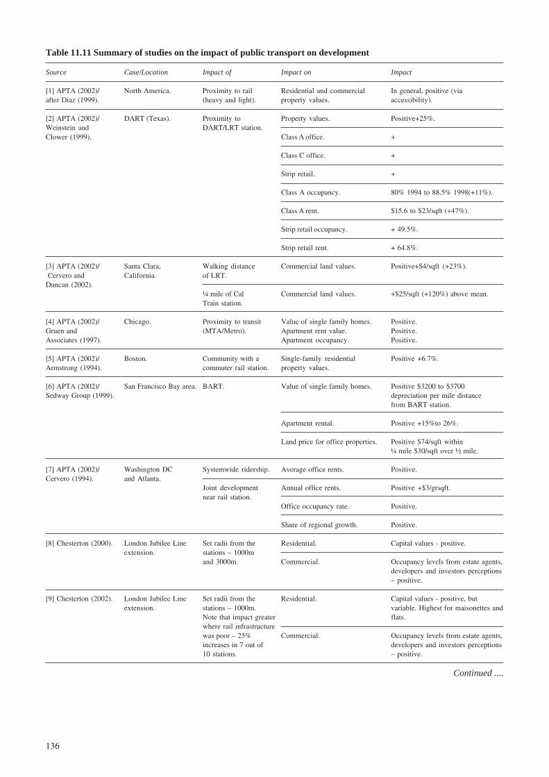
136

Table 11.11 Summary of studies on the impact of public transport on development

Source Case/Location Impact of Impact on Impact

[1] APTA (2002)/ North America. Proximity to rail Residential and commercial In general, positive (viaafter Diaz (1999). (heavy and light). property values. accessibility).

[2] APTA (2002)/ DART (Texas). Proximity to Property values. Positive+25%.Weinstein and DART/LRT station.Clower (1999). Class A office. +

Class C office. +

Strip retail. +

Class A occupancy. 80% 1994 to 88.5% 1998(+11%).

Class A rent. $15.6 to $23/sqft (+47%).

Strip retail occupancy. + 49.5%.

Strip retail rent. + 64.8%.

[3] APTA (2002)/ Santa Clara, Walking distance Commercial land values. Positive+$4/sqft (+23%). Cervero and California. of LRT.Duncan (2002).

¼ mile of Cal Commercial land values. +$25/sqft (+120%) above mean.Train station.

[4] APTA (2002)/ Chicago. Proximity to transit Value of single family homes. Positive.Gruen and (MTA/Metro). Apartment rent value. Positive.Associates (1997). Apartment occupancy. Positive.

[5] APTA (2002)/ Boston. Community with a Single-family residential Positive +6.7%.Armstrong (1994). commuter rail station. property values.

[6] APTA (2002)/ San Francisco Bay area. BART. Value of single family homes. Positive $3200 to $3700Sedway Group (1999). depreciation per mile distance

from BART station.

Apartment rental. Positive +15%to 26%.

Land price for office properties. Positive $74/sqft within¼ mile $30/sqft over ½ mile.

[7] APTA (2002)/ Washington DC Systemwide ridership. Average office rents. Positive.Cervero (1994). and Atlanta.

Joint development Annual office rents. Positive +$3/grsqft.near rail station.

Office occupancy rate. Positive.

Share of regional growth. Positive.

[8] Chesterton (2000). London Jubilee Line Set radii from the Residential. Capital values - positive.extension. stations – 1000m

and 3000m. Commercial. Occupancy levels from estate agents,developers and investors perceptions– positive.

[9] Chesterton (2002). London Jubilee Line Set radii from the Residential. Capital values - positive, butextension. stations – 1000m. variable. Highest for maisonettes and

Note that impact greater flats.where rail infrastructurewas poor – 25% Commercial. Occupancy levels from estate agents,increases in 7 out of developers and investors perceptions10 stations. – positive.

Continued ....

137

Table 11.11 (Continued) Summary of studies on the impact of public transport on development

Source Case/Location Impact of Impact on Impact

[10] Pharoah (2002) London JLE Note that sites close Residential. Development applications – variableto stations more impact by accessibility, potential andattractive to development history – positive, butcommercial and mixed in limited areas.use developments, andthose further from Commercial. Sites close to stations sought forstations more attractive mixed use and commercialfor residential developments.developments.

[11] Wrigley and Review paper. Multi sector. Residential and commercial Intra urban and regional, capturingWyatt (2001). property values. agglomeration and network effects.

[12] Hillier Parker London Crossrail Assumed impact area Commercial. Additional floor space of 10.87(2002). (projected). set at 1km from million sq metres by 2025.

the stations.Residential. 54,804 new dwellings in study area

by 2025.

[13] Henneberry Sheffield Supertram. Assumed impact area Residential property values. House prices reduced with(1998). at 1km along either anticipation of construction of tram

side of line. lines, but negative impactdisappeared after opening.

[14] Dabinett (1998). Sheffield Supertram. LRT. Non residential Unable to identify any discreteproperty value. Supertram influence.

[15] Dabinett (1998). Sheffield (and LRT. House prices. Influence so small that it cannot beManchester). separately distinguished.

[16] Laasko (1992). Helsinki. Metro and rail. Property values. Overall, +$550-$650 million gain invalue (US$, 1990 prices).

[17] TRL (1993). Tyne & Wear. Metro. House prices. 200m+2% above those further away.

[18] Wacher (1971). London Victoria Line. Metro. Property values. Values in catchment area of lineincreased between 1% and 5%compared with properties outside thecatchment.

Source: RICS Policy Unit (2002).

138

Table 11.12 Status of systems examined for theirobjectives

Country

City Type of system Status

AustraliaBrisbane Light rail AbandonedMelbourne Light rail OperationalSydney Light rail Operational

CanadaCalgary Light rail OperationalScarborough Automatic light rail OperationalVancouver Automatic light rail Operational

ChinaTuen Mun, Hong Kong Light rail Operational

DenmarkCopenhagen Automatic light rail Operational

SwedenStockholm Light rail Operational

SwitzerlandLausanne Light rail Operational

UKCroydon Light rail OperationalLeeds Light rail PlannedLondon Docklands Automatic light rail OperationalManchester Light rail OperationalNottingham Light rail Under constructionSheffield Light rail OperationalTyne and Wear Light rail OperationalWest Midlands Light rail Operational

USABaltimore Light rail OperationalDallas Light rail OperationalHonolulu Light rail AbandonedKansas City Light rail PlannedSacramento Light rail OperationalSan Diego Light rail OperationalSan Jose Light rail Operational

Source: Mackett and Edwards (1998).

The surveys upon which these data were based were carried out in1992-1994. The status information has been updated.

11.6 Conclusions

The relationship between land use and public transportdemand is complex. A number of different aspects of landuse can influence both the number and length of publictransport trips.

The higher the density of a city, the higher the demand forpublic transport in terms of ridership but the shorter the triplength. It should be recognised that factors such as highresidential density and attached (terrace) housing tend to beassociated with lower income households, whilst lowresidential density and detached housing tend to be associatedwith higher income households. In addition low incomes areassociated with low car ownership. Hence, at least part of theeffect of density on the demand for public transport will bedue these income and car ownership effects.

Settlement size, urban form and mix of uses all too havean influence on public transport use, although it is difficult

to establish the precise nature of these relationships. Themore the region is linked into the public transport network,the more viable each development becomes and the moreviable public transport becomes. Planning can be used toencourage this link through policies to encourageappropriate development types in appropriate locations.

Cities are decentralising, which tends to reduce thedemand for public transport. Hence, there is a need topromote public transport in order to maintain patronage inorder to counter the secular trends in decentralisation,suburbanisation, and increasing car ownership.

New public transport systems and their levels ofpatronage have implications for urban areas in terms ofeconomic and physical development. Evidence ofdevelopment impacts was found for the new systems in StLouis, San Diego, San Jose, Portland, Calgary, Vancouver,Rouen and Tyne and Wear. In these cases complementaryplanning and traffic management policies were used andthere have been at least some years since they opened whentheir national economies have not been in recession. In somecases this may be simply a matter of shifting developmentfrom one area to another, and therefore not necessarilyadding to the overall level of economic development in thecity. In other cases, it may be making the city served by thelight rail system more attractive than other cities withoutsuch a system, and so adding to economic growth locally,but not at a regional or national scale.

Table 11.13 Objectives of developing light rail systems

ToTo To serve

To reduce improve the Toimprove traffic the city stimulate

public conges environ centre developCity transport -tion -ment better -ment Other

Brisbane •Melbourne •Sydney •Calgary • • •Scarborough • • • •Vancouver •Tuen Mun, Hong Kong •Copenhagen • • • •Stockholm • • • •Lausanne • •Croydon • • • •Leeds • • •London Docklands •Manchester • •Nottingham • • •SheffieldTyne and Wear • • •West Midlands • • • •Baltimore • • •Dallas • • • •Honolulu •Kansas City •Sacramento • •San Diego • • •San Jose •

Source: Mackett and Edwards (1998).

The information in this table is based upon interviews and postalsurveys of experts involved in the development of the systems. For thelist of experts see Mackett and Edwards (1998). The surveys upon whichthese data were based were carried out in 1995-1996.

139

There are examples of public transport systems beingused as instruments of urban planning policy, with thedegree of success a function of the level of patronage. Thenature of planning and financial systems can influence thestrength of such relationships and the extent to which traveldemand can influence the development of urban areas

12 New public transport modes

12.1 Introduction

In this chapter we consider how public transport demandmight be affected by the introduction of new modes ofpublic transport, which may replace or supplement moreconventional modes. The modes considered are light railand guided busways, of which several examples have beenestablished over the last two decades, but are currentlybeing proposed as an important ingredient of modernpublic transport strategies.

In Sections 12.2, 12.3 and 12.4 we discuss the meritsand disadvantages of light rail systems, guided buswaysand Park and Ride; in Section 12.5 we present methods offorecasting demands for proposed new systems.

12.2 Light rail

12.2.1 The nature of light railLight rail is a modern form of public transport that runs onrails. It shares many characteristics with heavy rail systemssuch as metros and suburban rail, but has lower capacity.Its main advantage over these other systems is that it haslighter and generally smaller rolling stock. This enableslight rail to accelerate and decelerate more rapidly,negotiate tighter curves and steeper gradients, and have acloser station spacing. It is cheaper and more flexible.Light rail spans the range from Tyne and Wear Metrothrough Docklands Light Railway to the modern tramwaysoperating in Croydon and Manchester.

Light rail can run on a mixture of city streets andexisting railway routes, even sharing tracks with suburbantrains. It can be totally segregated from all other traffic,run at the margin or along the median of highways, or beoperated on the street in mixed traffic. Light rail can alsobe elevated or built in tunnel. Often a combination of theseis used to match local circumstances, for example by usingdisused railway embankments to provide a fast interurbanroute with street running in town centres.

Light rail usually has a much simpler signalling thanheavier rail systems, and, in its tramway form, relies on thedriver’s judgement in a similar manner to the driver of abus, particularly in mixed traffic conditions. When it isrunning along a highway it can be given priority atsignalised junctions.

Light rail is nearly always powered by electricity which isusually supplied through overhead wires, but can besupplied through a third rail system. The latter can only beused when the system is completely segregated from thepublic except at stations. It is also possible to have driverlessautomatic systems which also have to be segregated.

Table 12.1 Number of light rail systems and metrosopened since 1970

Light rail systems Metros

1970s 1980s 1990s 1970s 1980s 1990s

Western Europe 0 7 14 7 2 4North America 1 13 8 3 2 1Rest of the World 4 17 12 13 17 12

Total 5 37 32 23 21 17

Source: Babalik (2000) based on Taplin (1997, 2000).

In some ways light rail is simply a modern version ofthe tram, but in some cities, such as Amsterdam andMelbourne where there are extensive tram systems, lightrail lines are being built, often with some segregation, toprovide high speed links to areas not previously served bytrams. Generally, light rail is modern, has at least somesegregation from other traffic, and powered by electricity.New systems are usually the subject of extensivemarketing campaigns, and branded with a suitable namessuch as ‘Metrolink’ or ‘Supertram’.

12.2.2 The growth of light railLight rail has grown in popularity in recent years. Since1970, 61 metros and 78 light rail systems have opened asBabalik (2000) has shown, using data from Taplin (1997,2000). Given the complexity of definition it is difficult tobe clear which was the first modern light rail system.Rogers (1975) defines the system in Edmonton in Canadawhich opened in 1976 as the first, regarding all previousexamples as extensions to, or rehabilitation of, existingtram systems. Table 12.1 shows the number of new lightrail systems opened around the World since 1970. It alsoshows the number of new metros opened since 1970 forcomparison. The major difference between light rail andmetros are that metros operate on dedicated lines that aresegregated from other forms of transport. Metros also tendto operate mainly underground, with much heavier enginesand passenger carriages.

It can be seen that in the 1970s the number of metrosbuilt outnumbered the number of light rail systems. Sincethen the picture has reversed completely, with 69 new lightrail systems opened since 1980 compared with 38 newmetros. North America led this trend in the 1980s, butsince then most activity has been elsewhere. Now there aremore light rail systems than metros in Western Europe andNorth America (Babalik, 2000).

12.2.3 The financial performance of light railThe capital costs of light rail are high, but less than thoseof heavy rail or road construction. Babalik (2000) hascollected data on a number of systems around the World.This is shown in Table 12. 2. This shows data for 23 lightrail systems, plus five metros for comparison.

The light rail systems that were the most expensive toconstruct are the Vancouver Skytrain at £843 million andthe London Docklands Light Rail at £775 million. Both of

140

systems which ranged in cost from £7,372 million for theWashington DC Metro to £1,058 million for the MiamiMetro. These are noticeably higher (but in the case ofWashington DC, for a much longer system).

The most expensive schemes to develop in terms ofcapital cost per km of route, were the three automaticsystems in Scarborough (Canada), Vancouver and LondonDocklands at about £28 million. Next comes Edmonton,which was the first modern light rail system and thereforemay have had high costs because of its innovative nature.The other schemes range in cost from £6 million per km inSacramento to £22 million in Calgary. It may be noted thatthe metros range in cost from £32 million per km for Miamito £71 million for Los Angeles. The variation in capitalcosts arises because of the different types of structurerequired: tunnel, elevated or at grade, the existinginfrastructure (often disused railway track beds can bereused) and the quantity of utilities (gas, electricity, waterand telecommunications) that have to be moved (rail-basedtransport systems cannot run over utilities because if a utilitypipe or cable has to be repaired, the transport system cannotfunction, unlike a bus which can be diverted to anotherroute). It can be seen that, in general, light rail systems aremuch cheaper to construct than metros, which partlyexplains their increasing popularity as was shown in Table12.1. Putting it another way, the lower cost per km of lightrail means that it may be regarded as feasible to develop asystem in a city which is too small to support a metro.

The annual operating costs for the light rail systemsvaries from £5 million to £34 million for Los Angeles. Thevalues for light rail are generally lower than those for themetros, which range from £21 million for Los Angeles to£190 million for Washington DC. Whilst, in general,longer systems tend to have higher costs, there areexceptions: the San Diego Trolley is the longest light railsystem, but it does not have the highest operating cost.

The cost of a system is influenced by many factorsincluding its size. It is also useful to consider costs in termsof patronage, and to compare operating costs and revenue tosee how close to profitability the system is. Table 12. 3shows the capital cost per kilometre of route, the annualisedcapital cost per passenger, the operating cost per passenger,the fare revenue per passenger, and the farebox recoveryratio, which is the ratio of revenue to operating costs. Forcomparison, the five metros are also included.

The operating cost per passenger varies considerablyfrom £0.14 for Calgary to £2.49 in San Jose. To someextent, the high operating costs per passenger reflect lowpatronage levels. For example, the light rail systems in SanJose and Baltimore each carry only about 7 millionpassengers a year compared with over 20 million on theLos Angeles, San Diego, Grenoble, Nantes, Manchesterand Tyne and Wear systems (the last carries about 35million passengers a year). It does not necessarily matter ifthe operating costs are high if the revenue is also high. Therelationship between these two figures is expressed as thefarebox recovery ratio, which is the percentage ofoperating costs covered by fare revenue. It can be seenthat, of the systems listed, only Manchester Metrolinkcovers its operating costs. It is run privately under a

Table 12.2 The cost of light rail systems (and metros)

Capital Annualcost in operating Fare

Route £ million costs in revenueCountry length at 1998 1998 in in 1997City in km prices £ million in £ million

CanadaCalgary 29 643 6 n/aEdmonton 14 362 n/a n/aScarborough* 7 184 n/a n/aVancouver* 29 843 22 8

FranceGrenoble 18 247 n/a n/aNantes 26 271 n/a n/aParis 9 67 n/a n/aRouen 15 256 24 9Strasbourg 11 207 n/a n/a

SwitzerlandLausanne 8 70 n/a n/a

UKLondon Docklands* 28 775 n/a 12Manchester 31 176 9 13Sheffield 29 271 9 5Tyne and Wear 59 533 27 21

USABaltimore 49 503 15 4Dallas 32 353 18 n/aDenver 9 141 5 n/aLos Angeles 57 717 34 3Portland 24 309 15 3Sacramento 30 165 10 4San Diego 80 609 17 10San Jose 32 527 17 3St Louis 29 260 13 5

USA Atlanta 62 3679 63 20

MetrosBaltimore 25 1136 22 6Los Angeles 18 1278 21 1Miami 33 1058 32 9Washington DC 144 7372 190 n/a

Source: UK patronage figures are for 2001/02 and are from Departmentfor Transport (2003a), US patronage figures are for 2000 and are fromFederal Transit Administration (2003). Other patronage figures werefrom Bushell (1997), except for Calgary, Vancouver and Rouen whichwere obtained by Babalik (2000). Other data have been taken fromBabalik (2000).

* Indicates an automatic system. N/A indicates that data were notavailable. Capital costs represent the value of the investment in theyear 1998. All costs and revenues are in UK Sterling at 1998 priceswith currency conversions made using the purchasing power parityindex provided by OECD (obtainable from http://www.oecd.org//std/nadata.htm ).

these are automatic which adds to the capital cost becauseof the extra technology required and because the systemshave to be completely segregated. The most expensivenon-automatic light rail systems were in Calgary, LosAngeles and San Diego which all cost over £600 million.The cheapest system shown here is the 8 km system inLausanne in Switzerland which cost £70 million. It isworth noting that the capital cost of five new metro

141

franchise agreement, and there is no subsidy to theoperator. The private sector operator is only interested inoperating the system if a profit can be made. The nextnearest to making a profit is Tyne and Wear Metro inBritain in which 77% of the costs are covered. This is anolder system which is still publicly owned. After thatcomes the San Diego Trolley, which covers 68% of itscosts. The San Diego Trolley is interesting because it wasinitially built with no funding from the FederalGovernment, with funding coming from state petrol tax.This meant that construction could start sooner and thatvarious regulations, such as prohibition of importingvehicles could be avoided (Wolinsky, 1994). The SouthYorkshire Supertram in Sheffield was privatised inDecember 1997 and now receives no operating subsidy.

The metro systems do not perform any better financiallythan the light rail systems, with three of them coveringabout 30% of their costs through the farebox, and LosAngeles Metro only recovering 4%. In general, the lightrail systems perform better than the metros. This maypartly explain the growth in their popularity as discussedabove: they are cheaper to build and they perform at leastas well as a metro in financial terms.

It can be seen that some systems are nowhere nearcovering their operating costs, such as the light railsystems in Los Angeles, Portland and San Jose. This raisesthe question as to whether they were developed for non-financial objectives with the subsidy required regarded as acost to be paid in order to meet the objectives.

It is worth noting that a number of commentators,particularly in the US, have criticised the development oflight rail schemes for being extravagant and inappropriateuses of resources, even going as far as claiming that deceithas been used, for example in Dallas (Kain, 1990). Part ofthe problem has been that for a number of years the USFederal Government provided some funding for new urbanpubic transport systems, with the amount of fundingprovided a function of the predicted level of patronage.Hence there was an incentive for planners to be optimistic intheir forecasts of patronage. Pickrell (1992) demonstratedthat there were significant differences between the forecastlevels of patronage and those subsequently observed. Arelated concern is that money invested in light rail has notbeen well spent. Gomez-Ibanez (1985) examined the lightrail systems in San Diego, Calgary and Edmonton. He foundthat not only were rail-based systems more expensive toconstruct than bus-based systems, but that the operatingcosts were higher. The systems did increase public transportpatronage, but only modestly and at a high cost. Heconcluded that investment in bus-based systems would havebeen more cost-effective. Kain (1988) came to similarconclusions about the Los Angeles and Dallas systems.

As shown above, light rail is expensive to construct. Thecost varies depending on whether it is built at grade,underground or elevated. If land has to be acquired, thismay be very expensive, particularly if it is currentlyoccupied by housing or economic activity. A majorexpense, typically about one quarter of the total cost ofsystems built recently in Britain, is the movement ofutilities from under the road. Because the capacity of lightrail vehicles is high, it is possible to have low operatingcosts per member of staff, possibly lower than on buses.

When a new light rail system is developed, it is commonfor sophisticated information systems to be provided,typically showing the arrival time of the next three trams atstops and next destination on board the tram. Suchinformation can increase the perceived reliability of thesystem, making it more attractive to users. If the system issegregated from other traffic, predictions of arrival timesare likely to be more accurate than those for buses whichcan be affected adversely by congestion.

12.2.4 The expected effects of a new light rail system ondemand

A new light rail scheme will have both direct impacts as anew mode, and indirect impacts as an alternative to existingmodes, particularly the car. The provision of a new light railsystem will meet the travel demand for many trips byincreasing the range of modes available. Some trips willtransfer from existing modes, including car, bus, andwalking. Other trips will be generated: a new fast publictransport mode is likely to create trip opportunities that werenot possible previously by opening up new trip attractions

Table 12.3 Cost and revenue indicators for light rail(and metro) systems

Annualised Opercapital -ating Fare

Capital cost/ cost/ revenue/ Fareboxcost/km pass pass pass recovery

City £ million -enger £ -enger -enger ratio (%)

Calgary 22 1.27 0.14 n/a n/aEdmonton 26 2.92 n/a n/a n/aScarborough* 28 4.34 n/a n/a n/aVancouver* 29 1.67 0.53 0.19 38Grenoble 13 0.90 n/a n/a n/aNantes 10 0.86 n/a n/a n/aParis 7 0.32 n/a n/a n/aRouen 17 1.50 1.73 0.64 37Strasbourg 18 0.96 n/a n/a n/aLausanne 9 0.80 n/a n/a n/aLondon Docklands* 28 3.04 n/a 0.72 n/aManchester 6 1.05 0.69 0.99 143Sheffield 9 2.42 1.15 0.60 52Tyne and Wear 9 1.25 0.76 0.58 77Baltimore 10 5.87 2.14 0.53 28Dallas 11 2.65 1.66 n/a n/aDenver 17 2.42 1.09 n/a n/aLos Angeles 13 2.47 1.41 0.15 7Portland 13 2.15 1.23 0.25 20Sacramento 6 1.68 1.20 0.49 40San Diego 8 2.18 0.76 0.55 68San Jose 16 6.27 2.49 0.48 20St Louis 9 1.47 0.87 0.37 46Atlanta Metro 59 3.89 0.82 0.23 32Baltimore Metro 46 7.28 1.73 0.51 31Los Angeles Metro 71 8.57 1.72 0.06 4Miami Metro 32 6.46 2.40 0.67 29Washington DC Metro 51 2.85 1.13 n/a n/a

Source: Babalik (2000).

n/a indicates that data were not available. All costs are in UK Sterlingat 1998 prices. The capital cost has been annualised by discounting thecapital cost in the year 1998 over 30 years at 8%. This has been donefor all systems to allow comparisons. It is not necessarily how it wasoriginally done for economic evaluation of the scheme.

142

within a reasonable travel time, although the limited spatialcoverage of a new system will mean that such opportunitiestend to be focused in a limited number of corridors. Becauselight rail tends to be faster than other modes it will probablylead to a net increase in trip lengths. It will enable some ofthose without access to a car to reach work, shopping andleisure facilities that they could not reach within the timethat they were prepared to spend. A modern low-floor lightrail vehicle may mean that some people with disabilities areable to make journeys of a type that were previously almostimpossible. There may also be considerable novelty valuewhich generates trips for their own sake, with the newsystem becoming a tourist attraction in its own right. A newlight rail system is not likely to have much impact on thetime of travel unless an explicit decision is taken to operatefor longer hours than buses.

12.2.5 The example of Manchester MetrolinkManchester Metrolink is a light rail scheme in the countyof Greater Manchester in the north of England. It openedin April 1992. It was constructed by taking over themainline suburban rail lines to Bury and Altrincham thatwere in need of re-investment. These two lines are linkedby an on-street section, with a spur into ManchesterPiccadilly, the main heavy rail station in Manchester.Thus, the original system links Bury in the north andAltrincham in the south with Manchester city centre. Aspur to Salford and Eccles opened in 1999.

The demand for travel by public transport in GreaterManchester is shown in Table 12.4: it has generallydeclined during the 1990s. Patronage on Metrolink was 8.1million in its first year of operation, after which it grew toabout 12-13 million where it seems to have stabilised.Patronage on other rail services in Greater Manchester hasbeen fairly static. The fact the Metrolink overtooksuburban rail in terms of patronage shows that the latter isnot a very important mode in Greater Manchester. Bus isthe dominant public transport mode and it is generallydeclining. Even though most users of Metrolink formerlyused the bus, Babalik (2000) showed that the introductionof Manchester Metrolink did not seem to alter significantlythe long-term downward trend in bus patronage in GreaterManchester. This is partly because bus has such a largeshare of the market. Even by 1998/99 Metrolink only had5% of the market compared with 90% on the buses.

An alternative way of trying to see the impact ofMetrolink on the use of other public transport modes is to

compare what happened when it was opened with thetrends in comparable areas. Table 12.5 shows the changesin the numbers of public transport trips between 1991/2and 1992/3 in other metropolitan areas. Total publictransport trips declined by 7% in the other areas, comparedwith a 1% decline in Manchester, suggesting thatMetrolink may have helped to sustain public transportpatronage in Manchester. Conversely, train patronage inManchester fell by 16%, whereas it fell by only 3%elsewhere, suggesting that Metrolink may have attractedsome users from heavy rail services (The heavy rail linesto Bury and Altrincham closed in August and December1991 respectively, so this partly explains the decline inManchester). Bus travel in Greater Manchester declined by3% over this period compared with a 7% declineelsewhere, confirming the point made previously thatMetrolink has not had a serious detrimental effect on busesin Greater Manchester.

Table 12.4 Number of journeys by light rail, bus andtrain in Greater Manchester (millions)

1991 1992 1993 1994 1995 1996 1997 1998-1992 -1993 -1994 -1995 -1996 -1997 -1998 -1999

Metrolink - 8.1 11.3 12.3 12.6 13.4 13.8 13.2Bus 260 252 236 226 224 212 211 217Suburban rail 13.0 10.9 10.7 9.7 11.4 10.6 12.2 11.8

Total 273 271 258 248 248 236 237 242

Source: Department of the Environment, Transport and the Regions(2001a, 2001b).

Table 12.5 Total number of journeys in othermetropolitan areas outside London,1991/2 – 1992/3 (millions)

1991 1992-1992 -1993

Bus 1217 1130Rail 120 117

Total 1337 1247

Source: Department of the Environment, Transport and the Regions(2001a).

The other metropolitan areas are West Midlands, Merseyside, SouthYorkshire, West Yorkshire and Tyne and Wear.

Table 12.6 Number of passenger-km by light rail, busand train in Greater Manchester (millions)

1991 1992 1993 1994 1995 1996 1997 1998-1992 -1993 -1994 -1995 -1996 -1997 -1998 -1999

Metrolink - 53.0 72.6 78.6 80.8 85.6 117.0 153.3Bus 1226 1117 1138 1141 1081 1040 1041 1009Train 241.0 216.0 222.4 197.4 212.2 215.4 214.8 197.0

Total 1467 1440 1433 1417 1374 1341 1344 1323

Source: Department of the Environment, Transport and the Regions(2001a, 2001b)

As well as trips, the total distance travelled can beconsidered, as shown in Table 12. 6. It can be seen that in1998/99 Metrolink had 12% of the market, heavy rail 15%and bus 76%. The total demand for public transport hasdeclined over the 1990s, with bus declining fast, heavy railbetween 210 and 220 million in most years, and Metrolinkgrowing steadily. The faster rate of growth in total distancetravelled than the number of trips by Metrolink impliesthat the average trip length is increasing.

It can be seen that the opening of Metrolink coincidedwith a decline of 2% in total public transport patronage inGreater Manchester. This compares favourably with a 5%decline in other metropolitan areas (see Table 12. 7). It

143

should be borne in mind that this was a period of economicrecession in Britain. Total rail patronage in GreaterManchester grew by 12%, compared with a static positionelsewhere, which suggests that Metrolink helped rail travelto grow in Greater Manchester. Bus showed a 9% decline inGreater Manchester compared with a 6% decline elsewhere.Given that the number of bus trips in Greater Manchesterwent down less than elsewhere, this suggests that a numberof longer bus trips have been lost to Metrolink, but theremay be some more short trips being made by bus, possiblybecause of increased seat availability because of the transferof some longer trips to Metrolink.

with a 15% decline in the peak and a 3% growth off-peakin adjacent corridors. The Bury corridor is not so buoyantwith a 3% decline in the peak and 101% growth off-peak.This can be compared to a 21% decline in adjacentcorridors in the peak and a 109% growth off-peak inadjacent corridors.

Table 12.7 Number of passenger-km in othermetropolitan areas outside London,1991/2 – 1992/3

1991 1992-1992 -1993

Bus 5008 4685Rail 912 911

Total 5920 5596


The other metropolitan areas are West Midlands (bus only), Merseyside,West Yorkshire and Tyne and Wear.

Table 12.9 Change in rail demand in Greater Manchestercorridors, 1990-93

Peak Off-peakCorridor (07.00-10.00) (10.00-13.00)

Bury -3% +101%Northern corridors -21% +109%Altrincham +63% +166%Southern corridors -15% +3%

Source: Table 3.1 in Oscar Faber (1996a).

The northern and southern corridors exclude the Bury and Altrinchamcorridors.

Table 12.10 Comparison of estimated observed andforecast sources of Metrolink patronage

Estimated Originalobserved forecast

Mode proportion proportion

Car 12.5-14.8% 11.5%Bus 25.8-28.2% 19.9%Rail 57.0-61.1% 68.5%

Source: Table 5.3 in Oscar Faber (1996a)

Table 12.8 Number of passenger-km in GreaterManchester by car, light rail, bus andtrain, 1998

Passenger-km (millions) %

Car 13530 91Metrolink 117 1Bus 1041 7Rail 197 1

Total 14885 100


The Metrolink figure is actually for the financial year 1998/9. The carfigure is based upon the annual road traffic on main roads figure of 11billion, of which 80% are cars and assuming a car occupancy of 1.54,which is the national average, based on figures from Department of theEnvironment, Transport and the Regions (2001b).

It is possible to see how much Metrolink contributes tomeeting the total travel demand by mechanised modes. AsTable 12.8 shows, it is only about 1%. Car isoverwhelmingly dominant, with 91% of the market. Publictransport has only 9%. Hence, in overall terms Metrolink ismaking a very minor contribution to meeting travel needsin Greater Manchester. However, by its nature, light rail isvery location specific, so it will contribute much more thanthis in the corridors it serves.

This localised effect is illustrated in Table 12. 9. Thechanges in rail demand in the Bury and Altrinchamcorridors are compared with adjacent corridors. TheAltrincham corridor shows a 63% increase in the peak and166% increase in the off-peak. This compares favourably

According to Law et al. (1994) patronage was higher onMetrolink than the former British Rail lines because of:

� Higher service frequency.

� Better penetration of the city centre.

� The fare structure on Metrolink made many journeyscheaper.

The peak period patronage on Metrolink on the Buryline was lower than anticipated for two reasons:

� Price competition from buses.

� Higher fares than in the days of British Rail.

It is relevant to consider where the patronage on Metrolinkhas come from. Table 12.10 shows the estimated observedtransfer from the monitoring study carried out by Oscar Faber(1996a, 1996b). It can be seen that the majority havetransferred from rail, mainly the heavy rail lines thatMetrolink replaced. Just over one quarter have come frombus, and about 13% from car. This table does not include anytrips generated as a result of the existence of Metrolink. Thetable also shows the original forecasts of the proportions. Acomparison of the two sets of figures suggests that the transferfrom car and bus was underestimated in the forecasts and thatfrom rail was overestimated.

An alternative calculation of the modal origins of theMetrolink trips from the University of Salford MonitoringStudy is shown in Table 12.11. This makes the comparisonwith the situation which would have been expected if the

144

Bury and Altrincham lines had still been operated byBritish Rail. This is used rather than the ‘before’ situationbecause there was a gap of several months when neitherheavy nor light rail operated on these lines and a highquality bus service was operated, which may haveinfluenced travellers’ modal choice in the medium term.They estimate that there are 4.5 million more trips onMetrolink than would have used the heavy rail lines thatthey replaced. Of these, 2.6 million (58%) were previouslycar trips, 36% were bus trips, 4% used other rail lines, and4% were not made previously.

More recently Scheurer et al. (2001) claim thatMetrolink has taken 2.5 million car trips a year off theroads, equivalent to a 10% reduction in traffic on theMetrolink corridor (but possibly releasing space for othercar drivers, so that there might be no visible effect ontraffic levels). According to Greater Manchester PassengerTransport Executive (1995) Metrolink may have affectedthe pattern of car purchases in the area it served becausebetween 1991 and 1994, the number of cars per persondropped by 3% in the Metrolink corridor compared with arise of 5% in the county as a whole.

12.2.6 The example of South Yorkshire SupertramIn July 1976 the Sheffield and Rotherham Land Use andTransportation Study recommended the development of asegregated passenger transport system on six corridorsradiating from the centre of Sheffield which is a city in thenorth of England in the County of South Yorkshire. In1979 the six lines were safeguarded by South YorkshireCounty Council against conflicting development. In 1982-83 studies were carried out to consider alternative modes,followed by technical evaluation during 1984-85. InNovember 1985 a Private Bill was put before Parliamentseeking powers to develop and operate the system. Afurther Bill was deposited in November 1988 for a lineinto the Lower Don Valley to assist in regeneration.Financial approval was given by the Department ofTransport in December 1990. This required the setting upof two companies owned by South Yorkshire PassengerTransport Executive (SYPTE): one to own theinfrastructure and trams, the other to use the assets under aconcession agreement, with a view to privatisation at alater date. Construction took place from 1992 to 1994,with the first trams delivered in late 1993. The first linewas opened on 21 March 1994 from the edge of the citycentre to the Meadowhall shopping centre. The full systemwas opened by October 1995. In December 1997 thesystem was privatised with the bus operator Stagecoachtaking over operation of the system. This led to a numberof changes to the operation of the system, including newtimetable and fares package (Haywood, 1999).

The demand for travel by public transport in SouthYorkshire is shown in Table 12.13. Patronage onSupertram has not been as high as expected (Fox, 1996),but it has increased steadily as remedial action has been

Table 12.11 Estimated annual Metrolink patronage(millions) by previous mode

Controlsituation:

if Bury/Altrincham

linesMetrolink Metrolink still had Metrolink

forecast actual BR services impact

Not made ‘new trip’ 1.3 2.5 2.3 0.2Car 3.3 0.7 2.6Bus 3.0 2.6 1.0 1.6Rail 7.6 3.5 3.3 0.2Other 0.0 0.2 0.3 -0.1

Total 11.9 12.1 7.6 4.5

Source: Table 2 in Knowles (1996) from the Metrolink Impact Rail UserSurvey 1993.

Table 12.12 City centre impacts of Metrolink onhighway demands

% reduction in cars entering the city centre – AM peak 1.8%

% reduction in cars entering the city centre – off-peak 0.7%

Number of long-stay parking acts likely to have been removed 690

Number of short-stay parking acts likely to have been removed 520

Source: Table 6.5 in Oscar Faber (1996a)

Table 12.13 Number of journeys by light rail, bus andtrain in South Yorkshire (millions)

1991 1992 1993 1994 1995 1996 1997 1998-1992 -1993 -1994 -1995 -1996 -1997 -1998 -1999

Supertram – – – 2.2 5.3 7.8 9.2 10.4Bus 177 176 166 163 158 150 144 135Suburban rail 6 6 6 6 6 6 6 6

Total 183 182 172 171.2 169.3 163.8 159.2 151.4


Rail services are those supported under Section 20 of the 1968Transport Act.

Whilst there seems to have been quite a large transfer toMetrolink from the car, this does not necessarily mean thatthere will be a significant decrease in traffic flows becausesome people who were previously deterred from usingtheir cars because of congestion may start using them.According to Law et al. (1994) there is evidence that cartraffic has reduced in the Bury and Altrincham corridors,except in the peak period in the Altrincham corridor,where there has been little change. The effects arecomplex, but at that time (1993) it seemed reasonable toconclude that there had been some reduction in car use onroads parallel to Metrolink, but it was impossible tomeasure the effect precisely.

Oscar Faber (1996a) looked at the effects on highwaydemand in the city centre, as shown in Table 12.12. Theyconcluded that there had been a 1.8% reduction in thenumber of cars entering the city centre in the morning peakand a 0.7% decrease off-peak. They also concluded thatthere has been a reduction in the number of parking acts:690 long-stay and 520 short-stay.

145

taken. Total public transport demand in South Yorkshiredeclined throughout the period shown, and the opening ofSupertram has not reversed this trend, but it might haveslowed it down, since the decrease levelled off in 1993/94 to 1995/96. Bus patronage has been in long-termdecline, and it is not obvious that Supertram hasaccelerated this trend, a point confirmed by analysis overa longer period by Babalik (2000). Heavy rail demand inSouth Yorkshire is low, and appears not to have beenaffected by the opening of Supertram, which servesdifferent areas of the city.

This can be compared with the shift changes in patronageon bus and rail in other metropolitan areas at the timeSupertram was opened as shown in Table 12.14. In the otherareas there was a small growth in bus use whereas in SouthYorkshire there was a small decline, suggesting thatSupertram may have prevented a short-term growth in buspatronage in South Yorkshire which was probablyassociated with the improving economic situation at thetime. Rail showed a decline in the other areas whereas it wasabout constant in South Yorkshire at a very low level.

12.2.7 The effects of other systems on demandReference has already been made to a number of light railsystems around the World. In most cases, specificmonitoring studies have not been carried out, unlike theGreater Manchester and South Yorkshire systems, so it isnot possible to draw detailed conclusions about theirimpacts. It is, however, possible to take information fromthe surveys of light rail and similar systems by Mackettand Edwards (1998) and Babalik (2000). The Manchesterand South Yorkshire systems were included in bothsurveys and so will be included here where appropriate forcomparison.

One useful indicator of demand is how well actualpatronage matches that forecast since the forecast wouldhave been used as part of the planning process and to helpdetermine whether the project would be worthwhilefinancially. Table 12.16 shows the forecast and actualpatronage for a number of modern light rail systems.

Table 12.16 Forecast and actual patronage on aweekday for light rail systems in thousands

Forecast Actual%

City Year Patronage Year Patronage difference

Vancouver 1996 100.0 1996 136.0 +36%Manchester 1996 35.7 1996 44.5 +25%South Yorkshire 1996 70.7 1996 18.7 -74%Tyne andWear 1985 219.1 1985 208.9 -5%Buffalo 1995 92.0 1995 29.0 -68%Pittsburgh 1985 90.5 1992 31.1 -66%Portland 1990 42.5 1995 24.0 -43%Sacramento 1987 20.5 1987 12.0 -42%San Diego 1981 9.5 1981 12.0 +25%St Louis 1994 17.0 1994 44.4 +161%

Sources: Mackett and Edwards (1998) and Babalik (2000), usinginformation from Pickrell (1990), Dunphy (1995), Warren (1995),Federal Transit Administration (2000) and Department of theEnvironment, Transport and the Regions (2001b).

Table 12.14 Number of journeys in other metropolitanareas outside London, 1993/4 – 1994/5

1993 1994-1994 -1995

Bus 935 941Rail 109 100Total 1044 1041


The other metropolitan areas are West Midlands, Merseyside, WestYorkshire and Tyne and Wear (Greater Manchester has been excludedbecause of the introduction of Manchester Metrolink).

Table 12.15 Abstraction of Supertram trips from othermodes

%

New trips 12Car 20Bus 55Other modes 12

Total 100

Source: W S Atkins and ESRC TSU UCL (2000).

Table 12.15 shows where Supertram trips have comefrom. It can be seen that most trips (55%) have transferredfrom bus. 20% have come from car and 12% are new tripsthat would not have otherwise been made. Given thatpatronage on Supertram is low, 20% transfer from carwould not make a huge difference even if no othertravellers started using their cars because of the resultingreduction in congestion.

It can be seen in Table 12.16 that there are hugedifferences between the forecast and out-turn patronage. Outof the ten systems shown, patronage was overestimated infour cases and underestimated in six, with errors of up to161%. The one Canadian example, in Vancouver, was anunderestimate by 36%. As discussed above, on ManchesterMetrolink demand was underestimated by 25%, but asKnowles (1996) showed, the type of patronage forecast wasvery different to the actual, with much more off-peak traveland much less peak travel in reality than expected.Patronage on South Yorkshire Supertram has been wellbelow that forecast. Various reasons for this have beencited: the assumptions about the transfer from bus toSupertram were not realised (partly due to deregulation),new developments which were expected to generate anumber of trips did not take place (W S Atkins and ESRCTSU UCL (2000), and the way Supertram was operateddiffered from that expected (Haywood 1999). Forecasts forthe Tyne and Wear Metro were fairly close to the actualvalues, but the patronage declined after 1985, largely due toderegulation and the removal of feeder bus services andwere down to 126,900 per weekday by 1996.

146

The four US systems in which patronage wasoverestimated, in Buffalo, Pittsburgh, Portland andSacramento, were all constructed using some Federalfunding, giving some credence to the claim that patronagedemand was often overestimated under thesecircumstances. On the two other US systems patronagewas underestimated: San Diego Trolley which was initiallybuilt with no Federal funding and St Louis MetroLinkwhich was constructed after the funding rules werechanged.

Babalik (2000) has calculated the extent to which thetotal capacity of light rail systems is used, as shown inTable 12.17.

the systems have been the subject of some form ofmarketing and advertising even if it only coverage in thelocal press (adverse or otherwise), so a positive indicationin the table implies the implementation of the policy to asignificant extent, which is not necessarily the same aswhether or not it was effective.

Of the systems being considered here, only Vancouverand Manchester are considered to offer high frequencyservice. (High frequency is defined as being at least 10vehicles per hour in the peak and 5 vehicles per hour off-peak.) A travelcard is a period ticket which permits travelon all public transport modes in an area. The deregulationof buses in Britain (outside London) makes it very difficultto offer a travel card because it requires co-operationbetween companies whereas deregulation is designed toencourage competition. It is sometimes possible to offer aticketing system that offers travel on several modes in aderegulated environment, but it is unlikely to becomprehensive. Such a system has been tried in SouthYorkshire, but does not seem to have had a significanteffect. All the other cities outside Britain, except Portland,have implemented such systems. Competition legislationmakes it difficult to offer free transfer to buses on theBritish systems, but both the Canadian and three of the USsystems do so.

Three of the systems, Calgary, Portland and St Louisoffer some free travel. For example, free travel is offeredbetween six stations in the city centre off-peak on St LouisMetroLink. The idea is that it will encourage those whowould otherwise never use public transport to try it,thereby overcoming a mental barrier.

As mentioned above, all new light rail systems are likelyto be the subject of publicity, but some systems have beenthe subject of explicit marketing and advertising campaigns.All the North American systems were the subject of suchcampaigns, but in the case of Sacramento it seems to have

Table 12.17 Percentage of total capacity used on lightrail systems

City % of capacity used

Vancouver 38Manchester 33South Yorkshire 37Tyne and Wear 75Sacramento 33San Diego 55St Louis 45

Source: Babalik (2000).

The capacity used is the ratio of the average number of passenger tripsper hour to the total passenger carrying capacity of the systems per hour.

Table 12.18 Experience of the systems with operatingpolicies

SecurityMarketing staff on

High Free Some and boardfrequency Travel transfer free adver and at

System service -cards to buses travel -tising stations

Calgary � � � � �

Vancouver � � � � �

Manchester �

South Yorkshire ⊗ ⊗ �

Tyne and WearBaltimore � � �


Portland � � �

Sacramento � � �

San Diego � � �

St Louis � � � �

In Sheffield, introducing additional staff for ticket sale on board hasenhanced the security image of the system.



� It is not clear whether the policy has had any effect on theperformance of the system.


The figures in Table 12.17 look low, in general, becausethey are averages over the whole day, including reverseflows during peak periods. The highest values are foundfor the Tyne and Wear Metro, the San Diego and the StLouis systems, all of which have been the most efficient interms of matching supply to demand.

12.2.8 The use of operating and transport planningpolicies to increase demand

Two types of complementary policy that can help toenhance the benefits of a new light rail scheme will beconsidered here: operating policies and transport planningpolicies. The use of these policy instruments is consideredfor 11 systems: two in Canada (Calgary and Vancouver),three in Britain (Manchester, South Yorkshire, and Tyne andWear), and six in the U S (Baltimore, Los Angeles, Portland,Sacramento, San Diego, and St Louis) (Babalik, 2000).

The operating policies that are considered likely toenhance the benefits of light rail systems are:

� High frequency service.

� Travelcards.

� Free transfer to buses.

� Free travel on part of system.

� Marketing and advertising.

� Security staff on board and at stations.

The systems which are operated with these policies areshown in Table 12.18.

It should be recognised that some of these indicators arerather subjective and imply an assessment of the extent towhich the policy has been implemented: for example, all

147

been fairly ineffective. Of the three British systems, only inSouth Yorkshire has there been an extensive campaign, butit appears not to have been very effective.

Like many examples of publicly-owned infrastructure,light rail systems can be the subject of vandalism. Theycan also be perceived as dangerous for lone travellers,particularly after dark. All non-automatic systems carrydrivers usually locked in their driving cabs, partly for theirprotection. Thus the passenger areas are not activelysupervised, which offers scope for passengers to travelwithout a ticket with subsequent loss of revenue. For allthese reasons some systems have staff either at stations oron board. Whilst this increases costs, it can save money interms of revenue protection and reducing vandalism, andcan enhance revenue by encouraging those who wouldotherwise find travelling unescorted intimidating. Forexample, in South Yorkshire the ticket machines on thestations were subject to vandalism and there wasconsiderable revenue loss from non-payment of fares.Conductors were introduced which has helped to increaserevenue significantly.

The transport planning policies that are consideredlikely to enhance the benefits of light rail systems are:

� Integrating system into regional planning.

� Integrating system into existing urban projects.

� Locating stations at trip attractors or generators.

� Integrating bus services with new system.

� Providing car parking at stations.

� Restricting car parking in the city or in the CBD.

The systems which are operated with these policies areshown in Table 12.19.

The first two policies are to do with integration of thelight rail system into the existing infrastructure, either byincorporating it into a regional plan as happened inCalgary, Vancouver, Portland and Tyne and Wear, orincorporating it into an existing urban project, such asregeneration of an area, as has happened in Vancouver,Tyne and Wear, San Diego and, unsuccessfully, in SouthYorkshire.

A light rail system is more likely to be successful if itconnects two large centres which generate or attract trips,preferably over the whole day, to ensure a continuous highlevel of patronage. This happened in Calgary, Baltimore,Los Angeles, Portland, St Louis and San Diego. In all casesexcept the last it seems to have helped increase patronage.The effects are not so clear in the case of San Diego.

Buses can serve a complementary role to a light railsystem by acting as feeder services. This approach takesadvantage of the bus’s ability to go on any road, to collectpassengers to take to the light rail system which can thentake them into the city centre at high speed on a segregatedtrack. Buses can also be used as distributors if appropriate.This method is used for the North American systems. It wasused in Tyne and Wear until the buses were deregulated in1986. Since deregulation such services are offered only ifoperators perceive them as commercial opportunities orlocal authorities regard them as socially necessary. In theUK this has tended not to occur possibly because passengersprefer direct bus trips to their destinations rather than maketrips that require bus/rail interchanges.

The other two policies relate to car parking: providingcar parks at stations means that the light rail system can beused for park and ride. Restricting parking in the citycentre can make use of light rail relatively more attractive.Car parking has been provided at stations on all thesystems except Vancouver. In the British systems it doesnot seem to have been very effective. Only in Calgary hascar parking been restricted elsewhere as a policy toencourage light rail use.

Calgary seems to be the place where transport planningpolicies have been used most to encourage use of the lightrail system. In Britain, some policies have been tried, butthey do not seem to have been very successful, especiallyin Manchester and South Yorkshire. All the U S systemshave been the subject of at least two complementarytransport planning policies which seem to have beensuccessful.

12.3 Guided busways

12.3.1 IntroductionKerb-guided buses operate in a segregated buswayusing a guide wheel running along a kerb to steer thebus. The guideways allow buses to bypass congestedsections of the network, or take more direct routes. Thiscan result in both reduced journey times andsubstantially improved reliability.

Other traffic is prevented from using the guideway as ameans of overtaking slow traffic, parking or unloading, bythe barrier between the guideway and the general trafficlanes. Entrance to the guideway can also be controlled by

Table 12.19 Experience of the systems with transportplanning policies

Integr Locating Integr Restrict-ating stations -ating Provi -ing

Integrating system at trip bus -ding carsystem into attrac services car parking

into existing -tors or with parking in the cityregional urban gener new at or in

System planning projects -ators system stations the CBD

Calgary � � � � �

Vancouver � � �

Manchester �

South Yorkshire ⊗ �

Tyne and Wear � � � * �

Baltimore � � �


Portland � � � �

Sacramento � �

San Diego � � � �

St Louis � � � �

* Policy was implemented and was effective during the first 5 years ofthe operation of the system.



� It is not clear whether the policy has had any effect on theperformance of the system.


148

use of a remote signalling system that lowers a barrier asthe bus approaches. Additionally, the design of theguideway, with two concrete tracks separated by drainagechannel filled with coarse chippings makes it difficult forother vehicles to use. The axle width of cars is too narrow– thus one wheel would be on the track whilst the otherwould be in the drainage channel. The guideway isgenerally too narrow for lorries, with their wider axlewidth, to use. Smooth transition between the guideway andnormal carriageways is achieved using a funnel whichgradually steers the bus into the guideway.

A second type of guided bus system, sometimes referredto as guided light transit (GLT), is a hybrid between roadand rail (Smyth, 1994). The system is steered by aretractable roller mechanism, which runs in a central raillaid in the roadway. The rail is flush with the road surface.This system allows the benefits of a smoother journey tobe achieved on mixed-use streets as well as on theguideway. However, the vehicles can be five times moreexpensive than kerb-guided buses (Smyth, 1994).

Guided buses can also use standard busways and buslanes. Thus, at the end of the guideway, buses can go indifferent directions on the normal road network, thusallowing a greater number of destinations to be servedwithout the need for interchange. Buses may also be ableto leave the guideway part way along its length. Thereforea wide catchment area can make use of the improvements.This flexibility also allows the service network to adapt tochanges in demand over time.

Guided buses may prove more attractive to passengersthan conventional buses for several reasons:

� Accessibility – the use of the guide wheel allows thebuses to stop extremely close to the kerb or platformedge with only a small (50mm) uniform gap between thebus and the platform edge, allowing for easy levelboarding.

� Comfort – the combination of the high precisionconcrete track that the buses run along and controlledsteering from the guide wheel, provide passengers witha faster and smoother ride than can be achieved withconventional buses.

� Speed – speed gains are made in two ways: if a separateguideway is used then the guided bus can by-pass trafficcongestion. The guide system also adds to a fasterjourney, as steering is smoother around corners etc.

� Image – guided bus has the potential to be seen as a‘new’ mode, shaking of the image of the conventionalbus of slow, uncomfortable and dirty. To achieve thisthe scheme must be marketed in the right way,accompanied by strong branding and with considerationput into the design of the vehicles, the design of buspoles, stops and interchanges, and timetables etc.

However, these advantages come at a cost:

� The track is more expensive to construct than a standardbusway, which at its simplest only requires theconstruction of a barrier between the busway and themain carriageway.

� Buses have to be converted to use the system. Standardbuses can be used but must be fitted with guide wheels.This can add 10% to the cost of a new bus.

� The construction of the system prevents buses frompassing each other, therefore express services and localservices cannot usually be run at high frequencies alongthe same route. Although this will depend on the lengthof the guide way sections.

12.3.2 Examples of schemes in operationExamples of cities with kerb-guided bus systems includeEssen, Mannheim and Adelaide. The Trans val de Marne(TVM) busway in Paris is used by a Guided Light Train.There are also guided light train schemes in Caen andNancy, although both schemes have suffered from technicalproblems causing them to be temporarily shut down. ThreeUK cities have guided bus schemes currently in operation:Leeds, Bradford, and Ipswich. All these schemes are kerb-guided systems. The UK schemes differ from the Essen andAdelaide schemes in that the guideway operates on shortstrips at points where previously buses tended to get stuck intraffic queues. The schemes in Essen and Adelaide includelong stretches of uninterrupted guideway.

All the UK guideway schemes were constructed as partsof larger schemes to enhance the quality of a route orcorridor. Other enhancements included higherspecification buses, other bus priority measures, servicefrequency enhancements, street furniture design, generalenvironmental improvements such as new planting, andcustomer-care trained drivers. In addition the schemeshave been accompanied by strong image branding throughinitiatives such as specially designed bus stops and buspoles and the choice of bus livery.

Work started on the Ipswich Superoute 66 in 1993.Phase 1 began operating in January 1995 (Enoch, 1998).The route runs from Kesgrave to Ipswich and includes200m of guideway in both directions, and includes a bus-only link between Martlesham and Kesgrave. The firstLeeds scheme (superbus) which runs along Scott HallRoad (A65) opened in 1995. The East Leeds route,(branded elite) with guideways on York Road and SelbyRoad opened in November 2001. The guided busway inBradford was constructed as part of the Manchester roadquality bus initiative and opened on the 1st February 2002.

Costs for constructing an at-grade guideway are in theregion of £1 million per lane kilometre but will varydepending on ground conditions. The Leeds superbusscheme cost £750,000 in 1995 to construct 450m ofguideway, roughly £1600 per lane metre. This includesimprovements to street lighting, traffic signals, and theenvironment. Two ‘docking stops’ on adjacent highwaywere also included in the scheme. The cost of theguideway excluding these environmental improvementswas approximately £700 per metre (Enoch 1998). The costof fitting the buses to run along the route with guidewheels was £3000 per bus. The Ipswich scheme involved£2 million of investment in new infrastructure and £0.5mon new buses.

149

12.3.3 Effects on journey timesThe Leeds superbus scheme provided service timeimprovements of between 3 and 5 minutes during themorning and evening peaks, as well as improvements inthe reliability and punctuality of the services using theroute. The construction of the 450m outbound guidewayalong Scott Hall Road reduced variability in bus journeytimes by 75% (Daugherty and Balcombe 1999). TheIpswich scheme provided time savings of 3-4 minutes andagain produced significant improvements in punctuality.

12.3.4 Effects on demandPatronage on the Leeds superbus route increased by 45%after 1 year and by 65% since it began operating in 1995(FirstGroup, 2003). Daugherty and Balcome ( 1999)found, that of 1585 trips made by 340 weekday passengerssurveyed, that service improvements following theintroduction of the superbus had generated 90 journeys perweek, i.e. an increase in demand of 5.7%. Of these, over80% were by new users, the remainder being by existingusers changing the frequency with which they used theroute. Steer Davis Gleave (1997) cited in (Daugherty andBalcombe 1999) estimated a patronage growth on thesuperbus route of 3% relative to growth across the rest ofLeeds. The differences between these figures has not beensatisfactorily explained; it may be due partly to the timingof the various before and after data collection exercises,and partly to difficulties for interviewees in disassociatingreasons for change from bus service improvements.

The Ipswich scheme saw patronage grow along the routeby 21% in the first quarter of operation and by 75% sinceopening (FirstGroup, 2003). Numbers of passengers boardingbuses on the guideway section of the Manchester roadinitiative in Bradford rose by over 16% in the first 9 monthsof operation, whilst patronage in Bradford as a whole rose by6% over the same period (West Yorkshire PTE, 2003).

The experimental kerb-guided bus scheme whichoperated in Birmingham from 1984 to 1987, along a sectionof road which experienced relatively little traffic congestion,was reported to have experienced a rise in patronage 26%above that for other services within the city (Bain, 2002).

The passenger profiles of both the Leeds superbus andIpswich superoute 66 schemes are more like those for LRTthan for conventional bus (Enoch, 1998). Between 20 and25% of passengers on the Leeds superbus are car owners;between 10 and 20% of new passengers have shifted fromthe car (Bain, 2002). Of the passengers on superoute 6623% were former car users and 2.8% were newlygenerated (Enoch, 1998).

A number of stated preference studies were carried outby Steer Davies Gleave in the early 1990s. These studiesfound that car users reaction to guided bus expressed interms of generalised minutes ranged from -12 to -26depending on the details of the scheme. This compareswith a range of -21 to -29 for bus, -5 to -15 for light railand -8 to -22 for light rail (Kilvington, 1992).

12.4 Park and Ride

According to Parkhurst (1996) Park and Ride (P&R)usually has one or more of three aims:

� To maintain or increase the number of economicallydesirable trips to the city centre.

� To avoid using valuable city centre land for car parksand access roads.

� To reduce congestion and noise pollution.

Hitherto P&R has usually been implemented foreconomic rather than environmental reasons. Researchgenerally focuses on short-range P&R, which is usuallybus-based, as opposed to the traditional long-range rail-based P&R. The pioneers of short-range P&R tend to behistoric towns and cities. One of the problems withresearch into P&R is that it tends to start on a small scaleand has expanded incrementally. For example, between1997 and 2001 P&R use increased by 16% per annum(Menzies, 2002). New P&R sites will often attractpassengers from existing P&R sites and from bus services.For example, monitoring of the introduction of Oxford’ssecond P&R site, (admittedly only 7 months afterinauguration) found that a quarter of the users had alreadybeen travelling by P&R, half of those (an eighth overall)had switched from Oxford’s 1st P&R site, and the otherhalf (other eighth) ‘had been practising ad hoc park andride from the suburbs using scheduled bus services;perhaps an early indicator that what matters for the successof park and ride are not so much its intrinsic qualities, butthe perceived alternatives’. There is a problem with P&R’spoor ability to attract patronage in early years, thus itsefficiency appears poor, and has to be subsidised by localtaxpayers. Oxford’s fourth P&R site (Thornhill) opened in1985. It was found that due to its location it attracts usersfrom the conventional bus services, taking advantage ofcheaper fares. Around 40% are accessing the site on foot.

Cooper (1993) carried out a survey in York which foundthat a number of P&R users who had not previouslyconsidered using public transport would now do so. 60%of respondents had previously driven and 19% had usedthe local bus, now 35% said they would use bus if P&Rbecame unavailable. It was found that 22% did not accessthe P&R site by driving to it (2% travelled by bicycle, 15%walked, and 5% were going the ‘wrong’ way). It was alsofound that 12% had not travelled to York before P&Rbecame available.

Similarly, 20% of P&R users in Oxford on a Saturdayfelt they would not come to Oxford at all in the absence ofP&R. By introducing P&R it is easier to resist pressure toretain or increase parking capacity in city centre. It wasfound that as the area of a journey’s origin becomes morerural public transport is likely to become a less acceptablealternative to P&R. Parkhurst (1996) believes that ‘Parkand ride evolved as part of a strategy which sought topreserve accessibility. It has been successful in doing this,but by improving vehicle occupancy, not reducingcongestion. Perhaps if the sole aim of park and ride hadbeen reducing congestion, it would have been abandonedlong ago.’ P&R has tended to limit the increase in car tripsinto the centre of city, it does not usually diminish theactual number of car trips. P&R, however, may contributeto loss of patronage on services just outside the city, whichin already marginal cases could destroy their profitability.

150

Use of P&R tends to increase over time, as new sitesopen. Some of this increase may well be attributable torising car ownership, and also the generation of trips thatwere previously suppressed due to the road congestionbefore P&R (Parkhurst, 1998). One of the causes ofresistance to P&R use is concern about site security, andpersonal safety, particularly when returning after dark.Sometimes the reduced travel cost for P&R can maketravelling to a particular area more attractive, and result ina revival of that area’s economic fortunes. In the plans forthe pedestrianisation of the centre of Oxford, someretailers cited the provision of P&R as an importantelement of the future viability of the centre.

For P&R’s decongestion benefits to be realised it isimportant that:

i The provision of P&R sites should not lead to an overallincrease in parking space supply in the city.

ii Other users should not be attracted to the vacated roadspace.

To aid the latter, road restriction measures might beintroduced as soon as possible after the P&R is provided,preferably at the same time, before potential users haveadjusted to any increased capacity.

Politically, there can be a noticeable resistance to a newtransport initiative if the measures that restrict use occurfirst. For example, the building work to introduce buspriority measures and light rail schemes can cause a lot ofdisruption to existing services and road use, which canincrease people’s hostility to the scheme, as in the case ofSheffield Supertram (WS Atkins and ESRC TSU, 2000).

WS Atkins (1998) present data on P&R in 8 cities. Forthe 47% of users who said they would otherwise drive allthe way, they found their journeys by private car shortenedby 2km. Distance of site from City Centre was aninfluence here, the maximum possible was 4km onaverage. It was found that 63% (range 55% to 66%) ofusers had previously driven, 17% (range 10% to 28%)came from conventional public transport. It should benoted that a proportion of respondents reported ‘other’.

Parkhurst (1999a) notes that the net saving per carparked is 1.7km. Unfortunately, bus based P&R, tends tointercept motorists rather later in the journey (covering onaverage about 25% of the overall journey). On averagearound 62% (range 52% to 71%) of P&R users are in thetarget group (those who travelled to the town centre by carbefore P&R was introduced). Around 17% (range 8% to40%) previously used conventional buses and trains.Around 50% said that in the absence of P&R they woulddrive to the city centre. Around 27% (range 18% to 41%)said they would revert to or choose public transport if P&Rbecame unavailable. It is thought that around 12% of P&Rtrips are extra trips generated by the P&R. Earlier workhad suggested that trips to the city following theintroduction of P&R increased by between 2 to 11%. Somedelegates at the English Historic Towns forum of 1998suggested that P&R might in time be viewed as an interimphase ‘filling a breech’ until longer-distance publictransport services can be revitalised. Other people think itmight lead to an outer ring for a city.

Due to inter-centre competition, it is not often possibleto set P&R charges at a price that does not undercut publictransport. In other words in order to attract users to P&R itmay be necessary to charge less than the costs of providingit, but that may mean that P&R costs less to use then theconventional local public transport. Sometimes P&R isintroduced, because of: a temporary reduction in citycentre parking (for example on market day), or increaseddemand due to a festival attracting extra visitors fromoutside, or to compete with out of town shopping centres acertain times (e.g. Christmas).

It is suggested that small scale P&R sites should beintroduced far from the urban area, so that cars could beintercepted earlier, people could also access services bywalking or shared taxi, and several sites could be arrangedlike stations along a railway line so the same P&R buscould pick up passengers from several sites.

WS Atkins (1998) found that 16% would not have madetheir journey in the absence of P&R. Trip generation as aresult of P&R is particularly high in Brighton, Coventry,and, Reading about 18%, 21% and 18% respectively. Inthe other 5 cities trip generation was between 7 to 14%.

Parkhurst (1999b) uses the same calculations as WSAtkins to calculate P&R ridership, i.e. those who arrive atthe P&R site who would otherwise have driven all theway. Hence this does not consider people:

� mode-switching from longer-distance conventionalpublic transport to P&R use;

� travelling to other places instead of using P&R to thesame city;

� not travelling instead of using P&R;

� travelling short-range to a P&R site by car rather thanwalking to a more local bus service;

� travelling by car to the centre instead of using a modeother than car (cycle, walk) to access the P&R busservice (where permitted).

This means that only 47% of the WS Atkins sample fellin the category considered, 53% did not.

Parkhurst’s model used the estimated daily cost indistance travelled (weekday km) of providing a dedicatedP&R bus services to 18 sites in 8 cities. (1 each inBrighton (200 spaces), Coventry (450 spaces) and Reading(625 spaces), 2 in Plymouth (120 spaces), 3 each inNorwich (1530 spaces), Shrewsbury (1750 spaces) andYork (2000 spaces), and 4 in Cambridge (1700 spaces).This was factored by 3 possible equivalent passenger-carunits (PCUs) for bus (as Bus km x PCU). If the value of 3is applied then the distance travelled by buses to each siteis between 873 to 2,844 km per weekday, if the value 2 isapplied the distance is between 582 to 1,896 km perweekday. These figures (for each site) were then dividedby the number of users who avoided car use byinterchanging at the site (this was derived from patronagedata). The car km saved for each car parked was calculatedon average for each city. The car km saved, average car-equivalent km travelled by buses per car parked, and thedifferent between the two were all presented in a table,below. The difference was calculated as car equivalent buskm-car km saved, so if it is negative then there is a net

151

reduction in vehicle km as a result of P&R, but if it ispositive then the impact of the bus services is greater thanthe reduction in car-km (Table 12.20).

In order to make bus-based park & ride attractive, it isnecessary to offer an adequate frequency throughout theday. Where a route’s demand arises only from P&R sites,then a problem may arise if a site fills up in the morningpeak, since little off-peak ridership will be found. This ismore likely to be seen where constraints on site provisionrestrict total spaces that can be provided. Winchester can beseen as an example of this. It may be noted that bus-basedP&R provision in Britain is atypical of P&R provisionelsewhere, which is often rail-based (for example, on newlight rail systems) and hence the service level and ridershipare not solely dependent on P&R demand, even wherespecial stations may be provided for P&R traffic.

There is a question over whether non-motorists shoulduse the bus service or not. In some cases people using thebuses the ‘wrong way’ (i.e. coming from the city centrefirst and are likely to be non-motorists) are required to paya higher fare or prevented from using the bus by means ofthe ticketing arrangements. While this means that only the‘intended’ market is actually served, it also means thatlocal taxpayers, whether motorists or not are subsidisingmotorists. However, if the planners decide to make thescheme socially inclusive by allowing non-motorists to usethe services for the same fare means that the P&R schememay be in direct competition with the local conventionalbus service, which can have a detrimental effect on the

Table 12.22 Costs and benefits of park and ride schemes per day including site provision costs

Net Total Ticket Reductionvehicle-km net receipts per Net operating in vehicle-km

Cars per car change in Operational weekday (£) cost (£) per £, spentparked parked vehicle-km costs per

per per per weekday Car All Car All Car AllCity weekday weekday weekday (£) arrivers users arrivers users arrivers users

Brighton 590 -2.22 -1.313 794 833 1,282 -39 -488 Surplus SurplusCambridge 1,910 1.02 1,950 4,234 1,927 2,190 2,307 2,044 Net inc Net incCoventry 230 1.76 406 828 230 242 599 587 Net inc Net incNorwich 1,335 0.22 300 4,162 2,377 3,105 1,786 1,057 Net inc Net incPlymouth 1,492 -3.17 -4.735 2,252 1,265 1,405 988 847 2.71 3.15Reading 1,145 -6.51 -7,454 1,889 2,000 2,174 -110 -284 Surplus SurplusShrewsbury 3,046 -3.77 -11,472 3,859 2,332 2,455 1,527 1,405 7.51 8.17York 1,950 -1.08 -2,097 3,624 2,656 3,405 968 219 2.17 9.57

Source: Parkhurst (1999b).

Table 12.20 Comparison of car-km saved per carparked

Car-equivalentkm travelled Difference in

Car-km saved by buses car-equivalentCity per car parked per car parked km per car parked

Brighton -4.02 +1.80 -2.22Cambridge -1.50 +2.52 +1.02Coventry -1.66 +3.42 +1.76Norwich -3.46 +3.68 +0.22Plymouth -4.70 +2.16 -2.54Reading -8.54 +2.03 -6.51Shrewsbury -5.12 +1.35 -3.77York -3.26 +2.18 -1.08

Source: Parkhurst (1999b)

Table 12.21 Costs and benefits of park and ride schemes per day excluding site provision costs

Net Total Ticket Reductionvehicle-km net receipts per Net operating in vehicle-km

Cars per car change in Operational weekday (£) cost (£) per £, spentparked parked vehicle-km costs per

per per per weekday Car All Car All Car AllCity weekday weekday weekday (£) arrivers users arrivers users arrivers users

Brighton 590 -2.22 -1.313 732 833 1,282 -101 -550 Surplus SurplusCambridge 1,910 1.02 1,950 3,709 1,927 2,190 1,782 1,519 Net inc Net incCoventry 230 1.76 406 690 230 242 460 448 Net inc Net incNorwich 1,335 0.22 300 3,690 2,377 3,105 1,315 585 Net inc Net incPlymouth 1,492 -3.17 -4.735 1,907 1,265 1,405 642 502 4.16 5.35Reading 1,145 -6.51 -7,454 1,696 2,000 2,174 -303 -477 Surplus SurplusShrewsbury 3,046 -3.77 -11,472 3,319 2,332 2,455 987 865 11.62 13.27York 1,950 -1.08 -2,097 3,006 2,656 3,405 351 -398 2.83 Surplus

Source: Parkhurst (1999b)

It has been found that around 67% of the annualised costof providing P&R is the cost of providing the bus service,20% is the site operating costs and 13% is the notionalcapital cost of provision. Table 12.21 gives the costs andbenefits of P&R excluding provision costs. Table 12.22includes provision costs.

152

existing local services. It also means that the P&R serviceceases to become exclusive and dedicated. Possible waysround this include: operating the P&R service only in thepeak; if the site lies on an existing bus route combine thetwo (as in Reading); and, carefully consider location offuture sites so that they can be combined with existingservices. This still leaves unresolved the question aboutwhether P&R consumes resources that might otherwise beused to improve local public transport in general.

Parkhurst (2001) cites the English Historic Towns Forum(1993). Providing P&R and bus lanes may reduce roadcongestion and improve bus journey reliability making theconventional bus service more attractive to car users. It mayalso encourage car users who would not previously haveconsidered using public transport to do so, as it presentsthem with a positive image of it. To achieve this latter aimsome providers of P&R have tried to provide a high qualityservice, superior to that of the local bus service. Table 12.23gives the redistribution of passenger km between publictransport and a dedicated P&R service.

Trip Rate ModelsThese models are mainly used to forecast the demandassociated with a new rail station. The models assume thatrail demand is a function of the local populationsurrounding the new station and the forecasts are based onpatronage at stations in ‘similar’ areas to the proposed newstadium. The methodology is simple but takes no accountof the attractiveness of the destinations to be served. It iscrucial therefore that the stations used to estimate trip ratesare as similar as possible to the planned station. Sometypical trip rates for new stations in various circumstancesare outlined in Table 12.24.

Table 12.23 Redistribution of passenger-km between PTservices due to the provision of dedicatedP&R

Totalpassenger-km Passenger-km

travelled abstracted fromon P&R buses conventional Net change in

P&R scheme per weekday PT services passenger-km

Brighton 8,547 -2,808 5,739Cambridge 17,895 -5,536 12,359Coventry 1,343 -674 669Norwich 14,420 -17,133 -2,714*Plymouth 8,186 -3,835 4,351Reading 9,845 -5,844 4,001Shrewsbury 27,590 -15,297 12,293York 21,809 -16,234 5,575

* The negative value is correct, it is due to a high trip rate.

Source: English Historic Towns Forum (1993).

Table 12.24 Typical trip rates for new stations indifferent circumstances

Daily trips perthousand population % of

popu800m -lation

0-800m -2km fromfrom from beyond

station station 2km

Prime commuter belt on outskirts of urban centre 100 10 1Village areas surrounding urban centre 25 6 20Built-up areas close to urban centre 12 3 10Free-standing town 10 3 40

Source: ATOC (2002)

Table 12.25 Typical trip rates for new services indifferent circumstances

Daily trips per thousand populationwithin 2km of station

Inner suburban 10Intermediate / industrial 15Outer suburban 30

Source: ATOC, 2002

12.5 Forecasting demand for new services

The methodology used for forecasting the impact of newservices or new stations is very different to that used in forforecasting the effects of changes in rail fares or railfrequency. The framework for the latter is incremental,whilst for the former an approach that forecasts the absolutenumber of rail trips is required. The key parameters to beidentified in forecasting demand for new rail services are thegenerating potential of the origin station and the attractingpotential of the destination station, in addition to thegeneralised costs of travel between stations.

12.5.1 Forecasting modelsFour modelling approaches are put forward in the PDFH:

� Trip rate models.

� Trip end models.

� Direct demand models.

� Mode choice models.

Trip rates for new local rail services are shown in Table12.25 and are based upon evidence taken from five newservices. The services are low frequency (hourly) and thefares do not allow access onto other public transport modes.For areas such as London and PTEs these condition areunlikely and higher trip rates would be expected.

Trip end modelsThese models represent an improvement in the trip ratemodels with the consideration of other key explanatoryvariables. The PDFH quotes the example of a modeldeveloped for a route within Greater Manchester (Bury,Altrincham and Oldham/Rochdale services). The modeltook the following form:

90.92exp(0.00004 14.3i i iV P SV= −

0.0137 0.0000024 )i iRS BS+ −

where:V

iis the volume of rail travel from station i made bypeople walking to the station (daily boardings).P

i is the usually resident population within 2

153

kilometres of station i, adjusting for overlappingstation catchment areas.

SVi

is the proportion of population in social class V(head of household economically active and in anunskilled occupation. In 2000 only 2% of thepopulation were in this category).

RSi

is the number of rail departures per day fromstation i.

BSi

is the number of bus departures on roads adjacentto station i.

It is noted that the since this model was developed(1987/88) regional rail demand has increased by 45%(2000/01). In order to uplift the forecasts by this amountthe constant needs to be changed to 131.83. These types ofmodels are context specific and the PDFH recommendsthat specialist advice is sought when developing them.

Gravity or direct demand model

These models combine the observed aspects of traveldecision making (generation, distribution and modechoice) into a single direct model. The PDFH quotes amodel that was developed for local services within WestYorkshire and based on data for around 100 flows for1981/2. The model took the following form:

0.38 0.16 0.02 0.27 1.24 1.34243.72 1 2 1 /ij i i i j ij ijV P P P I II D GTR GTO− −=

Where:V

ijis the number of single rail trips between i and jand between j and i on an average autumnweekday.

P1i

is the usually resident population within astraight line distance of 800 metres of station i.

P2i

is the usually resident population within a straightline distance of 800 metres and 2 kilometres ofstation i (adjusted for overlapping catchments).

P1I/IIiis the proportion of population in P1

i in social

classes I and II (managerial and professional).D

jis the number of workplaces within 800 metres ofthe destination station divided by the number ofeconomically active residents.

GTRij

is the Generalised Time of Rail (in minutes) = 2(walk and wait time) + In-Vehicle Time + Fare/Value of Time.

GTOij

is the Generalised Time of Rail/(generalised timeof rail + generalised time of Bus + GeneralisedTime of Car.

The growth in regional railways passengers between1982 to 2000/01 (67%) means that the constant in themodel should be increased to 407.01. Once again thePDFH recommends that specialist help is sought whendeveloping such models.

Mode choice models

Most of these models take the form of a binary logit modechoice model that analyse separately choices between railand bus and between rail and car. Other models examinethe three modes simultaneously using hierarchical logit.

The variables used within the modes typically consist ofin-vehicle time, cost, access and egress time and serviceheadway for each mode being examined. Whilst they takeexplicit account of accessibility to the rail network, they donot usually allow choices between stations and betweenaccess modes to change the overall demand for rail.

The main weaknesses of these models is their inabilityto account for newly generated trips (principally in theleisure market) and the necessity to possess estimates ofdemand levels by other modes on the flows for which railforecasts are required. The PDFH does not recommend aspecific set of parameters. Instead it recommends that areasonably up-to-date model, estimated to broadlycomparable circumstances, is used for forecasting.

The PDFH recommends that specialist advice is soughtwhen constructing these models and that for large scaleschemes (re-opening of a new line with several stations forexample) a fresh mode choice study is conducted for thepurpose of forecasting demand.

13 Effects of other transport policies

The aim of this chapter is to assess the impact of a range oftransport policies not covered in detail elsewhere in thisguide. We start by considering transport policy objectiveswhich are broader than just focusing on demand issues. Wethen examine different transport policy instruments withrespect to these objectives, before looking at the specificimpact of these instruments on public transport demand.

13.1 The objectives of transport policies

There are a number of possible objectives of transportpolicies. The main objectives described by May (1997) aresummarised below (but see also www.elsevier.com/gej-ng/29/29/Konsult to see how these objectives have been usedin the knowledge base on Sustainable Urban Land Use andTransport, KonSULT).

Economic efficiencyThis objective seeks to maximise net economic benefit.With respect to public transport, it is normally defined toconsider revenue and costs to transport operators and thecosts and travel times of transport users (includingreliability). This definition assumes that there are noeffects external to the transport sector. A wider definitionwould include the additional costs and benefits ofenvironmental protection, safety, accessibility, economicregeneration, sustainability, equity and integration, manyof which are considered below.

Environmental protection

This involves reducing the impact of transport facilities, andtheir use, on the environment of both users and non-users.Impacts of concern are listed in the Design Manual forRoads and Bridges and include noise, atmospheric pollution,vibration, visual intrusion, severance, fear and intimidation,and loss of valuable objects e.g. flora and fauna, monuments(Department of Transport, 1993). An updated list in the

154

New Approach to Appraisal highlights CO2 emissions, local

air quality, landscape, biodiversity, heritage and water(Price, 1999). It is often argued that public transport hasenvironmental advantages over car based travel (see, forexample, TEST, 1991 and CPT, 2002).

SafetyThis considers reduction of loss of life, injuries and damageto property. Statistics indicate that public transport hassafety advantages over car based transport. (CPT, 2002).

AccessibilityThis can be defined as the ease of reaching facilities andcan be contrasted with mobility which is the ease ofmovement. The New Approach to Appraisal highlights therole of access to public transport, community severanceand the impact on pedestrians and others. Improvedaccessibility is often associated with the promotion ofsocial inclusion. It is often argued that public transport hasimportant benefits over car based travel in terms ofaccessibility. (CPT, 2002).

SustainabilityThis can be defined as development that meets the needsof the present without compromising the ability of futuregenerations to meet their own needs. It has become usualto consider sustainability, as consisting of three elements:economic, social, and environmental. As suchsustainability might be thought of as a high level objective.

Economic regenerationThis might be seen as re-inforcing land-use plans of thearea by promoting economic development in particularlocations. In certain circumstances, improved transportprovision may have benefits to the economy over andabove those measured by the economic efficiency of thetransport sector alone. This might be because transportimprovements increase competition in imperfect markets,either for final products or for factors of production(particularly labour and land). Alternatively, transportimprovements might promote economies of scale inproduction thus leading to reductions in production costs.The main impacts of public transport improvements arelikely to be on the markets for labour and land. Withrespect to the latter, an important recent report is that ofRICS Policy Unit (2002). In additional to objectives, it isalso important to recognise the role of constraints.

EquityThis means ensuring that benefits are equally distributed ortargeted to those with special needs. This may involve asocial element, such as concessionary fares for the elderlyand disabled, and/or a spatial element, such as subsidy forrural services.

FinanceCertain schemes may achieve policy objectives but areprecluded because they require high levels of capitalfinance or on-going revenue support.

Practicability

Certain schemes may achieve policy objectives but maynot be practicable because of lack of public support and/ortechnological barriers.

In the rest of this section, we examine five broad policyinstruments (land-use planning, infrastructure provision,infrastructure management, information provision andpricing) with respect to four objectives (efficiency,environment, safety and accessibility) and three constraints(equity, finance and practicability). An illustrativeassessment is based on a nine point scale but should not betaken as definitive. In particular, with assessments of thistype there is a danger of double counting. For example, areduction in public transport journey time may be seen as abenefit in terms of both economic efficiency andaccessibility. More up-to-date assessments will beprovided by the KONSULT database (see above).

These objectives can be pursued through a number oftransport planning instruments:

Land-use measures

Most land-use measures are designed to encourage use ofpublic transport, cycling and walking. Types of measureinclude: development densities, developments withintransport corridors, development mix, travel reductionordinances and parking standards (see also Section 11.3).

The possible impacts of land-use measures are shown inTable 13.1.

Infrastructure provision

This includes provision for the car e.g. new roadconstruction, new car parks, provision for public transporte.g. conventional rail, guided bus, light rail, park and ride,provision for cyclists and pedestrians e.g. cycle routes,pedestrian areas, and provision for freight e.g. lorry parks,transhipment facilities, encouragement of other modes.Possible impacts are shown by Table 13.2.

Management of infrastructure

Provision for the car includes: conventional trafficmanagement, urban traffic control, advanced transporttelematics, accident remedial measures, traffic calmingmeasures, physical restrictions on car use, regulatoryrestrictions on car use, parking controls, car sharing.Provision for public transport includes: bus priorities, highoccupancy vehicle lanes, bus and rail service levels, busservice management measures. Provision for cyclists andpedestrians includes: cycle lanes and priorities, cycleparking, pedestrian crossing facilities. Provision for freightincludes lorry routes and bans. Possible impacts are shownin Table 13.3.

Information provision

Provision for the car includes conventional directionsigning, variable message signs, real-time driver informationsystems and route guidance, parking information systems,telecommunications, public awareness campaigns. Provisionfor public transport includes service information, real-time

155

Table 13.1 Performance of land use measures

Objective measure Efficiency Environment Safety Accessibility Equity Finance Practicability Net

Density ? ? ? ✓ 0 0 × 0Corridors ✓? ✓? ? ✓✓ 0 0 × ✓✓

Mix ? ? ? ✓ 0 0 × 0Developer contributions 0 0 0 0 ✓ ✓ × ✓

Commuted payments ✓ 0 0 0 ✓ ✓ × ✓✓

Travel reduction ? ? ? ? 0 0 ×× ××Parking standards ✓ ✓ ? ✓/× 0 0 × ✓

Key✓ ✓✓ ✓✓✓ Positive impact on increasing scale.× ×× ××× Negative impact on increasing scale.✓/× Both positive and negative impacts.? Uncertain impact.0 No significant impact.

Table 13.2 Performance of infrastructure measures


New roads ✓? ✓/x ✓✓ ✓? ×× ××× × ×××Parking supply ✓? ✓ ✓ ✓? × × × 0Rail ✓✓ ✓✓ ✓✓ ✓✓ ✓ ×× ×× ✓✓✓✓✓

Light rail ✓✓ ✓✓/× ✓✓ ✓✓✓ ✓ ×× ×× ✓✓✓✓✓

Guided bus ✓? ✓? ✓ ✓✓? ✓✓ × ×? ✓✓✓✓

Park and ride ✓ ✓ ✓ ✓ 0 × 0 ✓✓✓

Terminals ✓/× ✓ ✓ ✓/× 0 ×× × ×Cycle routes 0 0 ✓✓ ✓ ✓ × 0 ✓✓✓

Pedestrian areas × ✓✓/× ✓✓ ×× ✓ ×× × ××Lorry parks 0 ✓ ✓ 0 0 × 0 ✓

Trans-shipment ? ? 0 ? 0 ×? ×× ××Other freight modes 0 ? ? ? 0 ×× ××× ×××××

Key: See Table 13.1.

Table 13.3 Performance of management measures


Traffic manage-ment ✓✓? ✓/× ✓✓ ✓/× ✓/× 0 0 ✓✓✓

Urban traffic control ✓✓ ✓ ✓ ✓ 0 ×× 0 ✓✓✓

ATT ? ? ? ? ? ? ? ?Accident remedial 0 0 ✓✓✓ 0 0 0 0 ✓✓✓

Traffic calming × ✓✓/× ✓✓ ×? ✓/× ×× 0 0Physical restrictions ××? ×? ✓? ×? ? 0 ×? ×××Regulatory restrictions ✓? ✓✓ ✓✓ ✓✓/×× ✓/× × ×× ✓

Parking controls ✓ ✓ ✓✓ ✓/× ✓/× 0 × ✓✓✓✓

Car sharing 0 0 0 ✓ 0 0 × 0Bus priorities ✓✓ ? ✓ ✓/× ✓ 0 × ✓✓✓

HOV lanes ✓? ? ✓ ✓/× ✓ 0 × ✓

Service levels ✓ ✓ ✓ ✓✓ ✓ ×× × ✓✓✓

Service manage-ment ✓✓ 0 0 ✓✓ ✓ × ×× ✓✓

Cycle lanes 0 0 ✓✓ ✓/× ✓ 0 0 ✓✓✓

Cycle parking 0 ✓? ✓? ✓? ✓ 0 0 ✓

Pedestrian crossings ✓ ? ✓✓ ✓ ✓ 0 0 ✓✓✓✓

Lorry routes, bans × ✓/× ✓ × ✓/× 0 × ×××


156

passenger information, operation information systems.Provision for cyclists and pedestrians includes staticdirection signs, tactile paving. Provision for freight includesfleet management systems. Possible impacts are shown inTable 13.4.

PricingProvision for the car includes vehicle ownership taxes, fueltaxes, parking charges, congestion charging. Provision forpublic transport includes fare levels, fares structures,concessionary fares. These have been considered inChapter 6. Table 13.5 shows the possible impacts.

13.2 Infrastructure management

13.2.1 Partnership between transport operators andpublic authorities

The bulk of this section draws heavily upon work carriedout by ITS and TSU as part of a project currently inprogress for the Department for Transport entitled QualityBus Partnerships (QBPs) and Market Structure. One of thetwo key project aims is continually to monitor thedevelopment and performance of QBPs in the UK via aseries of in-depth interviews with the relevant localauthorities and operators and other parties involved. Thesecond is to model QBPs under a number of differentcompetition and market structure scenarios. Phases oneand two of the project have been completed and along withthe ongoing work by TAS (2000), who carry out a biennialsurvey of operators and local authorities for inclusion intheir annual Bus Industry Monitor, they constitute the mostup to date in-depth review of QBPs.

According to TAS (1997) QBPs can be defined as:

‘An agreement (either formal or informal) betweenone or more local authorities and one or more busoperators for measures, to be taken up by more thanone party to enhance bus services in a defined area.’

Typically, the local authority provides traffic managementschemes, which assist bus services, while the bus operatoroffers better quality in various dimensions. The need forpartnership stems from the fact that no one organisation hascontrol over all the factors, which can improve the quality ofbus service provision to the customer. For example,improvements to reliability will often be dependent on theimplementation and enforcement of bus priority measures aswell as ensuring the delivery of the scheduled bus service.Similarly maintenance, provision and quality of bus stops andtraveller information may not be within the operators’ control.

Previous studies have reported a large variety in thenumbers of QBPs that exist ranging from two dozen(Hoban, 2000) to one hundred (Rye, 1999). This illustratesthe problem that can exist if a definitive definition is notadopted. Many of the QBPs identified by Rye were veryinformal and in many cases were possibly uni-lateral, e.g.operators taking it upon themselves to introduce highquality rolling stock. To make the definition more preciseTAS (1999) has outlined a number of principal elementsthat must exist in a QBP these are:

� The actions are designed to improve the attractivenessof bus use.

� There is agreement on the actions to be taken.

� ‘Both sides’ will be contributing in some way.

� The actions relate to a specific route or area.

Table 13.4 Performance of information measures


Direction signing ✓ 0 ? 0 0 × 0 0Variable message signs ✓? 0 0 0 0 × 0 ×Driver information ✓? 0 0 ✓ ×× ×× × ××××Parking information ✓ ? ? ✓ 0 × 0 ✓

Telecommunications ✓ ✓✓ ✓ 0 0 ×? ×? ✓✓✓

Public awareness ? ? ? ? ? 0 0 ?Timetables ✓ ? ? ✓✓ ✓✓ 0 ×× ✓✓✓

Passenger information ✓ ? ? ✓ ✓ ×× ×× ×Operation information ✓✓ 0 0 ✓ ✓ ×× ×× 0Fleet manage-ment ✓ 0 0 ✓ 0 × × 0


Table 13.5 Performance of pricing measures


Ownership taxes × × 0 0 ✓ ✓✓✓ 0 ✓✓

Fuel taxes ✓ ✓✓ 0 0 ✓ ✓✓✓ 0 ✓✓✓✓✓✓✓

Company car tax changes ✓✓ ✓✓ ✓✓ 0 ✓✓ ✓✓ 0 ✓✓✓✓✓✓✓✓✓✓

Parking charges ✓? ✓? ✓? ✓/× ✓ ✓ × ✓✓

Congestion charges ✓✓ ✓✓ ✓ ✓✓/× ✓✓/× ✓✓✓ ×× ✓✓✓✓✓✓

Fare levels ✓ ✓ ✓ ✓✓ ✓✓ ××× × ✓✓✓

Fare structures ✓✓? ✓ ✓ ✓✓ ✓✓ × × ✓✓✓✓✓

Concessionary fares 0 0 0 ✓ ✓✓ ×× 0 ✓


157

There is potentially a degree of tension between theQuality Partnership concept, at least in some applications,and competition law. Relevant legislation (Fair TradingAct, 1973, Restrictive Trade Practices Act, 1976 and theCompetition Act, 1980) severely restricts the freedom ofoperators to co-operate with one another (Mackie andPreston, 1996). A report for the Office for Fair Trading(1997) provides a useful review of the effectiveness ofregulatory policy towards the bus industry. The newCompetition Act (1998) has clear criteria for theexemption of individual and block agreements. These musteither improve production or distribution or promotetechnical or economic progress. Agreements must not‘impose on the undertakings concerned restrictions whichare not indispensable to the attainment of these objectivesor afford the undertakings concerned the possibility ofeliminating competition in respect of a substantial part ofthe products in question’ – Clause 9. Some of thesetensions were meant to be rectified by the 2000 TransportAct which made provisions for statutory partnerships.However, at the time of writing there is only one statutorypartnership in existence (in Birmingham). The vastmajority of partnerships are informal agreements.

The first phase of the Department for Transport projectincluded a series of interviews with the QBP partners in sixcase study areas. The interviews were designed to befactual in terms of identifying the financial and physicalinputs and outputs (Table 13.6), organisational in terms ofthe organisation of QBPs (Table 13.7) and subjective (didthe partners deem them a success etc).

The findings from the six case studies were broughttogether in the phase one report (Institute for TransportStudies and Transport Studies Unit, 2000). The keyfindings are summarised below:

� There is a clear preference for voluntary partnerships. Itis felt that voluntary QBPs have improved relationshipsand enhance understanding between local authoritiesand operators.

� QBPs are setting new standards for the industry.

� QBPs have encouraged bus operators to target theirinvestment strategies and operators have contributed toinfrastructure investment.

� QBPs have led to patronage growth, usually in anotherwise declining market. However, identifying thereasons for growth is difficult given a lack of detailedsurvey work.

� Leadership and effective project management are seenas critical to the success of QBPs. The ability to bid formanagement resources within the Local Transport Planwould be welcome.

� Marketing is seen as a key factor in achieving patronagegrowth.

� QBPs occur in conditions of mature competition,normally with one or two dominant operators.

� QBPs have been subject to limited, short-runcompetition in certain areas.

� There are widespread problems with enforcement of buspriorities. Although efforts have been made to includepolice forces, they are very much a ‘missing’ partner.Decriminalisation of parking offences is seen as only apartial solution, while moving offences remain theexclusive domain of the police. It is felt that the policedo not have any incentive to prioritise the enforcementof bus priorities.

� A constraint on the further development of QBPs is theposition of the OFT on competition in the bus industry.Further integration of services and ticketing will notoccur while operators perceive the threat of legal action.

Evidence on changes in patronage was presented byMackie (2000) in a paper given to a workshop on London’sBus Contracting Regime. The performance appears to beimpressive if one considers the national backdrop of fallingbus patronage (with the exception of London). Thepercentage rise in patronage differs across QBPs, areflection of the different features and background trends ofeach QBP. For example, two of the most ambitiousschemes, Line 33 and Scott Hall Road have enjoyed thelargest patronage growths. Other schemes such as Brightonhave been assisted by increasing population density in thecity centre and parking constraints. In fact all the schemespresented in the table are located in prime bus markets,reducing the investment risks to each party (Table 13.8).

Table 13.7 Organisational features of quality buspartnerships

Organisational features

1 Parties to the partnership.

2 Period covered.

3 Status of the agreement – formal, informal etc.

4 Area the QBP is applicable to – route, area, project specific or a widerstrategy.

5 Funding requirements & arrangements.

Source: Adapted from TAS (1999)

Table 13.6 Quality bus partnership inputs and outputs

Inputs Outputs

1 Journey times.

2 Service frequencies.

3 Reliability.

4 Traveller information.

5 Comfort/accessibility.

6 Fares/interavailability.

7 Entry/exit.

8 Tender market.

1 Traffic Priority – bus lanes, signal priority,bus gates, bus only roads & allowedmanoeuvres, pre signals, guideways,automatic vehicle location etc.

2 Information & Promotional Measures –real time passenger info., roadsidedisplays, joint promotional campaign,route branding etc.

3 Passenger Infrastructure – signage,shelters, at-stop facilities, interchangeimprovements, raised kerbs, improvedpedestrian access to stops etc.

4 Vehicles & Quality – new buses, low floor,low emission standards, alternative fuels etc.

5 Service, Fares & Tickets – enhancedfrequency, operational standards, service &fare simplification, new ticket products etc.

Source: Adapted from TAS (1999).

158

In total, Mackie (2000) finds that QBPs can increase bususage on average by 22%, but with a range of 5% to 60%.These results are consistent with later work by LEKConsulting (2002) which found eleven urban QBPschemes had an average uplift on bus demand of 21% witha range from 4% to 92%. CPT (2002) examined seventeenexamples of quality improvements with a mean passengeruplift of 33% (with a range from 10% to 72% - seeAppendix to Chapter 9).

Knowles (1999) found low cost QBPs only increaseddemand by between 5% and 8%. Comprehensiveconventional upgrade led to increase of demand ofbetween 10% and 30%, whilst major upgrades with someguideway could increase demand by over 40%. Of theeleven schemes analysed by Knowles, the averagepatronage uplift was found to be 20%.

13.2.2 Restricted access zonesUnited Kingdom examples of restricted access zonesinclude the Nottingham zones and collar scheme and theCambridge Core scheme. The Nottingham schemeattempted to discourage traffic entering the centre ofNottingham through signal delays. Signals at all junctionsaround the central area were set with long wait times andshort go times for traffic entering the area. The scheme ranbetween 1975 and 1976. No significant changes wereobserved in the mode of transport used by residents anduse of the park and ride scheme provided for visitors to thecity was low (Cairns et al., 1998).

The Cambridge core scheme has gradually restricted itscentral area to traffic by closure of three through routes.Phase 1 (closure of Magdalene St., Bridge St., and JesusLane) was implemented in January 1997. WS Atkinscarried out before and after surveys of traffic counts,journey speeds and journey times in June/July 1996 and1997 (Cairns et al., 1998). Traffic within the city fell byapproximately 10%, and by 44-48% along the affectedroute. Traffic on the ring road increased by 10%. Amodelling exercise carried out using SATURN to forecastthe impacts of the scheme suggested a 3-10% reduction intraffic in the central area.

In Oxford bus patronage has increased over the last 10years by 40% (Cairns et al., 1998). However, Oxford hasimplemented a mixture of policies ranging from theclosure to traffic of several streets within the centre,parking restrictions and introduction of bus lanes and parkand ride.

Rome introduced a limited access zone (LTZ) in 1994 incombination with parking fees (Sta spa, 2000). Residentsof the LTZ were given free permits to both move and parkwithin the zone. Authorised non-residents have beenrequired to pay for permits since 1998. In 2001approximately 70,000 permits were distributed (30% toresidents, 30% to non-residents, 30% to disabled, and 10%to freight vehicles). Public transport use has declinedbetween 1996 and 1999. The rate of decrease in suburbanand peripheral areas was 20%, whilst only 10% for trips to/from the centre.

Table 13.8 Estimates of patronage change in QBPs and associated features

% Change in Time ExplanatoryQuality bus partnership patronage period notes Associated features

Leeds – Scott Hall Road +60% * 1995-99 In the context of a Segregated bus way; bus lanes; traffic prioritymeasures; new lowdecline city wide. floor buses; route branding; increased service frequency;

increased information and publicity; driver training.

Nottinghamshire +29% 1st year. +48% since inception Bus lanes; new buses; increased service frequency; driverCalverton Connection in 1998. training; route branding.

West Midlands:Line 33 (Birmingham) +30% 1996-97 There has also been Line 33 – Traffic priority measures; bus lanes; real timeBloxwich (Walsall) +18% 1998-99 a +8% increase on information; new low floor branding; increased passengerPrimeline (Coventry) +5% 91998-99 the Bloxwich corridor. information and publicity; increased service frequency; driver

training.Bloxwich – Bus lanes; improved passengerinfrastructure; new low floor buses; increased passengerinformation and publicity; driver training.Primeline – Bus lanes;improved passenger infrastructure; new low floor buses;increased passenger information and publicity; driver training.

Edinburgh Greenways +12% (First) August LRT increase is set Traffic priorities; bus lanes (greenways); increased passenger+7% (LRT) 1997 against a 3% network information and publicity; improved passenger infrastructure.

onwards. decline.

Cheltenham Route 2 +5% September In context of a 1% Traffic priorities; bus lanes; new buses; improved passenger1998 network decline. infrastructure – note not all of features are in place as yet.onwards.

Brighton +5% Per annum Increased passenger information and publicity; improvedfrom 1995 passenger infrastructure; new vehicles (some low floor); driveronwards. training; increased frequencies; route branding.

Source: Mackie (2000).

* Note that this figure is contested. Daugherty and Balcombe (1999) only found a demand uplift of around 6%.

159

In September 1982 traffic restraint was introduced intocentral Athens. Private cars were banned from the citycentre. Buses, shared taxis and motorcycles were permittedto use the restricted zone. This was accompanied by an‘alternate day’ policy on car use within the central area.Odd and even number plates were permitted to enter thearea on alternate days. The restriction was in forceMonday to Friday 6.30 to 16.00, but was lifted for majorholidays and during the summer months. Initiallycommuters moved to public transport modes and use ofshared taxis. After one year of operation, traffic wasbanned totally from the inner ring, and the alternate dayrestriction zone was expanded outwards to cover a widerarea. In 1984, bus journey times were found to havereduced by 6.2% in the morning peak, 7.1% for outboundjourneys in the afternoon peak and by 1.7% off-peak. Asmall change was observed in bus use – a maximumincrease of 5%, with bus use in the inner area making up8.8% of mode share before the introduction of the schemeand 9.0% in 1984. Most of the displaced car journeysmoved to shared taxi or motorcycle.

Other European schemes include Bologna, whichintroduced a traffic-limited zone in 1972. This resulted in anincrease in bus patronage of between 38% and 66%depending on the route and bus speed increases of between15 and 20%. However, the zone was implemented alongsideassociated parking restrictions, park and ride facilities andpublic transport improvements (Cairns et al., 1998).

13.2.3 Road space reallocationRoad space reallocation involves changes to the types oftransportation activities that can use the road space. Roadspace reallocation may be undertaken to smooth the flowof specific modes such as bus priority lanes, cycle lanesand HOV lanes; to improve the quality and safety of thelocal environment (e.g. pedestrian improvements, trafficcalming). It has also been suggested that road spacereallocation can be used as a traffic reduction measure. Notall the displaced traffic will divert to neighbouring streets.Other possible responses include changing mode, changingdestination, trip chaining, changing journey time, notmaking the trip or making the trip less frequently.

Cairns et al. (2002) examined the evidence from anumber of case studies where roadspace had beenreallocated, for a variety of planned permanent, plannedtemporary and unplanned reasons. They found vehicleflows changed by between +25% and -146%. In somecases traffic disappeared both from the altered route butalso from the alternative routes. This may be a result of thecumulative effect of a number of traffic policies. Themedian reduction was 10.9% (mean = 21.9%).

Evidence from Chapter 9 suggests that in urban areasover 70% of this suppressed demand might switch topublic transport, reducing to 50% for inter urban travel. Inboth cases, these abstraction rates are net of re-routing andre-timing effects.

13.2.4 High Occupancy Vehicle lanesHigh occupancy vehicle (HOV) lanes restrict traffic usingthese lanes to vehicles with an occupancy of two or more

(in some cases higher). Some HOV schemes allow singleoccupancy vehicles to use the HOV lanes on payment of atoll; these are sometimes referred to as high occupancy toll(HOT) lanes. High occupancy vehicle lanes can affectpublic transport in several ways:

1 Increase traffic speeds, giving improved journey timesand thus reduced generalised costs of travel by publictransport compared with single occupancy vehicles, whichcould result in increased patronage.

2 In order to be able to make use of the HOV lanes, cardrivers may offer lifts to people who previously usedpublic transport. The extent to which this will occur willdepend on the time savings available from using the HOVlane compared with the delay incurred in stopping to pickup passengers.

A study conducted by the University of Pennsylvania(Vukic, 1995) comparing different lane priorityconfigurations found that bus patronage increased the mostwhen a lane on a road without HOV or transit prioritylanes, was converted for exclusive bus use. The worst-casescenario for public transport was to add a HOV lane on aroute which already had a bus only lane. This finding issupported by evidence from the El Monte busway in LosAngeles. The El Monte busway was opened in 1973 fortransit only. It was later opened additionally to carpools (3plus persons). Although the additional vehicles using thelane have not had an adverse effect on the running time ofthe buses, ridership levels have declined (Silver, 1995).Silver attributes this to the price of parking, length ofcommute and other factors which have made carpoolingmore attractive to many commuters than taking the bus.

UK experience of HOV lanes is limited. Evidence fromthe introduction of a HOV lane during peak hours on asection of the A647 in Leeds suggests a slight increase inbus patronage 5 months after the scheme was introduced(Leeds City Council, 1999). The number of scheduledbuses running in the morning peak has also increased.

13.2.5. Bus priority measuresSlinn (1993) lists the following bus priority measures:

� With flow bus lanes.

� Contraflow bus lanes.

� Busways.

� Bus only roads.

� Selected banned turns.

� Oneway streets/street closures.

� Signal rephasing (passive priority).

� Selective vehicle detection at signals (active priority).

� Queue relocation.

� Pre-signals advance bus areas.

� Waiting and loading restrictions/priority route treatment(e.g. Red routes).

� Bus stop treatments/bus boarders.

Introducing a bus priority scheme in north east London(Route 43) along with a red route scheme, which aims to

160

keep traffic moving by restricting parking and stopping,resulted in journey time savings and improvements inreliability of Route 43. Patronage on the route increased by8.8% to 8700 passenger journeys per week (Thompson,1993). Over the same period London-wide bus patronagedecreased by 2%.

Daugherty et al. (1999) examined a number of buspriority schemes including Aberdeen and Brighton. Theyfound no correlation between the bus priority schemelength and bus journey timesavings. The savings weremore likely to depend on the number and severity of thebottlenecks along the length of the scheme, rather than theoverall scheme length. The patronage data Daugherty et al.managed to obtain was ‘sketchy’, so the authors wereunable to draw any definite conclusions (but see alsoChapter 7). However, the journey time improvementsachieved by the schemes reviewed were of less than 5minutes, which is small compared with overall journeytimes. Therefore, the authors felt that bus priority schemeswould have limited impact on bus patronage levels.However, perception maybe important; the image of a busovertaking queuing traffic may help stem or reverse adeclining patronage. For example, the Brighton schemeresulted in a 16% increase in patronage as a result of acombination of things: the introduction of a flat fare, theenhanced image of the buses and priority measures. TheAberdeen scheme generated a 1.4% increase in patronage,from a combination of new travellers and increased triprates of previous travellers. However, this figure has awide margin of error due to the small sample size, i.e. onecan be 95% confident of a true patronage increase ofbetween 0.5% and 4.5%.

Other studies give higher trip generation values still.During the first year of operation super route 66 in Ipswichsaw a 20% increase in bus services along the corridor. Theroute includes 200m of guided busway and a number ofother bus priority measures including a bus gate whichpermitted more direct routing through a large residentialarea. The project also included promotion of the superroute and new buses (Handsley and Butterwick, 1999). Bythe fourth year of operation passenger numbers were 75%above those of the first year of operation.

13.3 Employer subsidies

In the US there is a growing trend to try and persuadeemployers to subsidise their employees’ use of publictransport, just as they do private transport, and in bothBritain and the US there have been moves to try andrestrict employer subsidisation of private transport. In1992 the National Energy Policy Act restricted USemployers to a maximum of $155 in parking subsidies. InNew York alone employees were getting free parkingworth an average of $200 a year.

One method for encouraging employer subsidisation ofpublic transport use is the provision of environmentaltravelcards, such as RTD Denver’s Eco Pass, (Trommer et al.,1995) an environmental travelcard purchased by employerson behalf of their employees. There is a group discountvarying with the number of passes purchased in a mannersimilar to health insurance. It is up to the employers whether

they then charge their employees for the pass; they maycharge from nothing up to the full cost of the pass.

Another, more popular method, for encouragingemployer subsidisation of public transport use, especiallyamong smaller employers for whom a pass from a specificoperator is both prohibitively expensive, and not reallysuitable, is a scheme such as TransitChek, (US Departmentof Transportation, 1995), where the employer purchasesvouchers from the appropriate organisation (TransitCentrein New York, DVRPC (Delaware Valley Regional PlanningCommission) in Philadelphia), which they pass on to theiremployee’s as a tax free-benefit (neither employer oremployee pays any tax on it. The employer may give thevouchers to all employees with their payslips, or only tothose that sign-up for it (some employers offer a choicebetween subsidised parking and TransitCheck), or as abonus or reward for good performance or attendance.TransitChek type options have only become a realisticpossibility in the United States since the 1984 DeficitReduction Act, which allowed employers to providevouchers towards the cost of travel up to $15 month ($180 ayear) as a de minimus fringe benefit (that is one that is toosmall to warrant taxation or associated record keeping). Costof living expenses meant this allowance was increased from1 July 1991 to $21 a month ($252 a year), and The NationalEnergy Policy Act increased it to $60 a month ($720 a year)from 1 January 1993. The employee then uses the voucherstowards the cost of purchasing a pre-paid ticket or tokens fortheir commuting travel. The employer has some choice overthe value of the vouchers they distribute monthly (rangingfrom around $15 to $60 a month). The schemes aregenerally too small as yet to have had a big impact onridership overall, but they seem to be fairly popular withemployees and in participating firms can go a long waytowards reducing commuting by car. For example a surveyamong participating companies in Philadelphia found thatbefore TransitChek was introduced 73.7% of employeesused public transport, 20.3% drove alone and 3.9% drovewith others. Afterwards 98.7% used public transport, 0.4%drove alone, and 0.6% drove with others.

Travel vouchers have been investigated as a way ofreducing fares in Great Britain. Root (1999) speculates, onthe basis of surveys in Oxfordshire, that the take-up oftravel vouchers might be 3.6% of the population in urbanareas but 7.2% of the population in rural areas. She notesthat research in the United States suggests such voucherscan increase public transport usage by between 30% and50%. This might suggest such a scheme could increase bususe for the journey to work by around 3% in rural areas.

13.4 Congestion charging

The idea of congestion charging has gained increasingpopularity over the past decade because of growingenvironmental pressures to curb greenhouse gas emissionsand improve local air quality, as well as economicpressures to reduce congestion; whilst the availability ofkey new technologies (such as smart-cards) has enabledsuch schemes to be implemented efficiently andeffectively. It has been shown to be particularly effectivewhere the revenue generated is ploughed back into further

161

improvements to the public transport system. Singaporehas been operating such a scheme since 1975.

During the early 1990s Norway implemented urban roadpricing schemes in several of its cities: Bergen, Trondheimand Oslo – charging for access to central areas, although theofficial justification for the Oslo scheme was not to restraintraffic but to generate revenue to pay for major roadinvestments (Hall, 1995). In Sweden, a toll ring wasproposed for Stockholm as part of a package of transportmeasures – the ‘Dennis Traffic Agreement’ (Tegnér, 1994).The scheme was to help finance new transport infrastructureas well as restrain traffic in the inner city. (This scheme waseventually abandoned for political reasons).

The UK Government is now following suit, andintroduced legislation to allow local transport authorities tocharge for road use and commercial car parking space inorder to reduce city centre congestion. The recentTransport Acts for England and Wales and for Scotlandgive local authorities the power to introduce congestioncharging, while the Greater London Authority Act 1999grants similar powers to the mayor.

There are two basic variations of road user charging:route-based schemes – charging for use of individualstretches of road; and zone-base schemes – charging usersto enter a bounded zone.

13.4.1 Route based schemesRoute-based schemes involve charging tolls for the use ofindividual stretches of road and have already beenimplemented in the UK as a way of recoupingconstruction costs for some bridges and tunnels. Untilrecently tolls have only been set for short stretches of thenetwork and where alternative no-pay routes areavailable. The new West Midlands’ Northern Relief Roadis a toll-route, with charges aimed at both recoupingconstruction costs and ensuring a free flowing routearound the West Midlands. The M1-M6 route around theconurbation remains free of charge.

UK empirical evidence on the effects of road tolls ontravel behaviour is limited. There have been two pilotstudies (Leicester and Bristol) both aimed at reducingcongestion and improving the environmental quality of thecities involved (Crawford, 1998). In the Leicester trials,which ran from August 1997 to May 1998, users werecharged for time using the A47, a main arterial route intothe centre of Leicester, during peak hours. The chargingpilot was accompanied by the opening of a park and ridescheme on the A47 corridor and bus improvements. Thetoll for using the route was varied from £2 to £10 (Ingreyand Fouracre, 1999). On average (for all charge levels) 2%of participants changed from using the car to the bus, 15%shifted from the car to park and ride, 25% changed theirroute and 13% changed the time at which they travelled.The numbers changing their travel behaviour variedaccording to the charge level. For example, at a toll of £2to £3 18% of participants in the trial changed route; thisincreased to 38% when the toll was raised to £10.

Trials in Stuttgart (Ingrey and Fouracre, 1999) of bothcorridor and cordon tolls found that a route-based schemeperformed better in terms of reducing traffic levels. This

was mainly due to the pricing scheme; once a user hadpaid to cross the cordon subsequent trips within the cordonwere not influenced by the pricing scheme. A maximum of5% of all trips transferred to public transport under thevarious scenarios trialled. However, each scenario wasonly piloted for two months, so medium to long-termeffects were not realised within the trial period.

A trial charging car users to use a corridor in the suburbsof Florence, resulted in similar levels of mode shift to thetwo examples given above, with 5% of car users changingto public transport to avoid paying the tolls (op. cit.).

A recent report by the Commission for IntegratedTransport (CfIT, 2002b) recommends that a national roadcharging scheme be implemented, with differential ratesbased on congestion levels. Charges would be distance-based. It was estimated that such a scheme would lead to20% traffic reductions in central London, traffic reductionsof around 12% in outer London and the metropolitanconurbations (e.g. Birmingham) and around 8% in citiessuch as Leicester. Traffic levels on motorways and ruralareas would reduce by less than 3%.

13.4.2 Zone based schemesThere are two main variants of zone-based schemes – (1)cordon toll schemes where road users are charged to crossthe zone boundary, in either one or both directions; and (2)area licensing schemes, where users purchase a licence tomove within the zone. Zone based schemes can beimplemented either through the display of a disc in the carwindow to show eligibility to enter a zone or throughsmart cards activated every time the car crosses the zoneboundary. The London area licensing scheme implementedin February 2003 works by comparing licence plates ofvehicles photographed inside the zone with a registry ofvehicles that have either paid to enter the zone or areexempt from the charges.

13.4.3 Modelling studies – UKThere has been some research on the effectiveness of roadcharging schemes in reducing traffic and on the optimalprice level to obtain maximum traffic reduction withminimum economic impact (e.g. Liu and McDonald, 1999).Most of this research has been conducted with the use oftransport models employing price elasticities to determinethe extent of modal switching, trip reduction and changes indestination choice. In many of the studies the effect ofcongestion charging is difficult to isolate as it was modelledas part of a package of transport improvements.

The MVA (1995) study on congestion charging forLondon is one exception. A variety of different cordon-based charging schemes with different prices for inboundand outbound traffic at different times of day weremodelled. No road or public transport improvements wereincluded. Bus trips were estimated to increase by between1.2% and 10.1% over the base, depending on the schemeand the level of charging. Most schemes were modelledwith low, medium and high levels of charging equatingroughly to £2, £4 and £8 charges. The smallest increase inpatronage was as a result of a scheme that charged for

162

crossing a central London cordon in either direction, withcharges ranging from 0p to £1.00 depending on thedirection and time of day. The largest increase inpatronage resulted from a two cordon scheme, with anadditional charge for crossing a screenline of the Thames.Motorist incurred an £8 charge for entering the centralLondon cordon and a £4 charge for crossing the InnerLondon cordon in peak hours. Patronage changes for railranged from -0.1% to 4.2%

The MVA study used an equilibrium model based on theMEPLAN-LASER model for the south east. The numberof rail services was assumed to be fixed, whilst for busesthe occupancy rate was assumed constant, with more busesbeing laid on to cope with any increase in patronage. Toavoid the virtuous circle of increased services leading todecreased wait times and thus a further increase indemand, an increase in the number of buses was assumednot to affect service frequency. Buses were assumed to runin convoy. Sensitivity analysis suggests that the modeltended to slightly underestimate bus patronage as a resultof these assumptions.

More recently, the ROCOL (2000) report on roadcharging options for London, modelled the effect ofintroducing an £5 area licensing scheme for the centralarea of the capital. With no public transport improvements,public transport patronage increased by 7% during themorning peak. This was composed of a 3% increase in railpatronage, 1% increase in underground use and a 2%increase in bus use.

Cooper et al. (2001) used a traditional four-stagetransport model to test a variety of different transportpolicy scenarios for Belfast, several of which included theintroduction of a toll cordon. One of the scenariosmodelled the impact of the toll cordon if introducedunaccompanied by supporting land use and transportinfrastructure improvements. This resulted in a 6%increase in transit passenger mileage compared with thedo-nothing scenario. When the toll cordon was combinedwith densification along major transport routes andimplementation of a number of high-quality publictransport schemes, it resulted in a reduction in transitpassenger mileage. With the addition of a city-centreparking levy, public transport passenger mileage rose by12% compared with the do-nothing case.

13.4.4 Modelling studies – internationalA study (Johansson and Mattsson, 1995) of the effect ofimplementing the Dennis Agreement in Stockholm, whichincluded increased rail track capacity, construction of a lightrail scheme and bus service improvements; as well ascompletion of a ring road. The charging scheme was to takethe form of a toll ring, with traffic charged for using the ringroad or entering into inner Stockholm. A network-basedequilibrium model (EMME/2) was used. The study foundthat under conditions of moderate economic growth thenumber of trips made during the morning peak by publictransport increased by 8% over 1990 levels. In the referencecase (no road tolls and only a modicum of public transportimprovements), public transport trips increased by 6%.

As already noted in Section 13.2.2, Rome introduced a

limited access zone (LTZ) in 1994 in combination withparking fees (Sta spa, 2000). The city is consideringimplementing road pricing for the LTZ. In preparation forthis several different road pricing schemes have beenmodelled, including road pricing replacing accessrestriction, charging residents an annual fee, and chargingmoped users. Most of the scenarios also considered somepublic transport improvements. The largest increase inpublic transport use was as a result of introducing a chargefor mopeds. 10% of car users switched to public transportwhen a per trip fee of €€ 3 rather than current flat annual feeof €€ 300 was charged. The amount of switching doubledwhen the per trip fee doubled. Seven percent of residentsswitched to public transport when a €€ 300 residents annualfee was introduced – currently residents are exempt fromany fees. Sta spa found that if road pricing is to replace theaccess restrictions, €€ 32 would need to be charged toachieve the same mode split of 20% public transport.

Oslo is also considering moving from an urban toll tocongestion pricing (Sorlie, 2002) when the 15 year tollperiod ceases. The Municipality of Oslo has undertaken astudy focussed on the design of the charging system. Theassumption was that the present toll ring is kept. One of thesystems modelled as part of the study involved charging anincreased toll during the morning and evening peaks (overdouble the current rate). The between-peak period wouldbe charged for at the current rate, and during low-trafficperiods the charge would be zero. It was assumed thatpublic transport capacity would be increased to handlemore traffic. This scenario resulted in an increase in theannual demand for public transport of 9.7% during themorning peak, 10.5% during the evening peak, 3%between peaks and -0.6% during low-traffic periods;giving a total annual increase of 5.3%.

Calthrop et al. (2000) modelled a series of congestioncharging/parking tax options for Brussels. They found thatintroducing a cordon toll to enter the CBD would increasethe share of peak hour trips made by public transport from20% to 24%, with no discernable effect on off-peak trips.

13.4.5 Before and after studiesThere is little UK evidence of the effect of congestioncharging on mode split. Durham’s cordon-based scheme witha £2 entry fee to the penisula section of the city has reducedtraffic by 90% (Parking Review, 2002). In London, sixmonths after the introduction of the cordon charge, thenumber of motor vehicles entering the zone during chargingtimes has dropped by 16%, and traffic delays due tocongestion have fallen by around 30%. Bus capacity has beenincreased to accommodate 15,000 extra bus passengerstravelling to the zone in the morning peak period (Transportfor London, 2003). Otherwise there have been a few trialroute-based schemes. However, as already mentioned thereare a number of schemes internationally that are in operation.

Ramjerdi (1995) estimates that the Oslo cordon tollscheme resulted in a growth in public transport patronageof 5%. This estimate was based on a before-and-afterstudy; the before study took place in October/November1989, and the follow up study a year later. The toll schemecame into force in February 1990. The results of the

163

survey showed a 6% decrease in the number of publictransport trips reported. However, the survey as a wholeshowed an 11% decrease in trips. Ramjerdi suggests thatthe reduction in trips was a result of significant under-reporting in the second survey. In addition the results arelikely to be affected by a period of recession that had beenaffecting the region since 1987, producing downwardtrends in employment, petrol sales and car ownership.There were also reductions in the levels of various cartravel subsidies between the 1989 and 1990 surveys.Ramjerdi compared her results with those from two otherstudies on the Oslo toll scheme, which reported a 0%increase in public transport trips between Apr 1990 andApril 1991, and a 0% to 3% increase in public transportuse based on ticket sales (Vibe, 1991; Nordheim andSælensminde, 1991; both cited in Ramjerdi, 1995).

Ramjerdi went on to estimate mode choice elasticitieswith respect to toll costs for different travel purposes usinglogit models (Table 13.9).

said that the cost of parking or lack of available space wasthe main reason for using the bus.

However, parking policies are not always effective trafficdemand management tools. Strict enforcement is required asthe tendency for evasion is high (Button, 1993).

13.5.1 Restriction of parking spaceMcSheen and Tweedale (1993) investigated the effect of aparking restraint policy for St. Albans using the SATURNmodel with elastic assignment of trips, based on responsesfrom 350 stated preference questionnaires from city centreemployees who drive to work. The traffic managementpolicy modelled included reduced levels of offstreet parkingthrough planning permissions – resulting in a rise from 33%of commuters without a private parking space provided to40-45% of total commuter demand. The policy modelledalso included provision of 5 park and ride sites, andimprovement of bus services along four corridors leadinginto the town centre. Between 475 and 495 morning peaktrips were transferred to bus in the short term (1996), risingto 540-620 trips in the long term (2006).

13.5.2 Parking pricingTRACE (1999) provides detailed cross-elasticity estimatesbetween parking price and public transport demand forvarious trip purpose, based on numerous European studies.The key finding is summarised in Table 13.10.

Table 13.9 Public Transport choice elasticities withrespect to toll costs

Journeys crossingAll journeys toll cordon

Journey to work 0.03 0.04Other travel purposes 0.02 0.05

Source: Ramjerdi (1995).

[Compare with cross elasticities in Chapter 8] Table 13.10 Cross-elasticity between parking price anddemand for public transport

Journey purpose Number of trips Kilometres

Commuting +0.02 +0.01Business +0.01 +0.00Education +0.00 +0.00Other +0.04 +0.02

Total +0.02 +0.01

Source: TRACE (1999), Table 8 and Table 9.

Table 13.11 Mode split and parking bay demandelasticities with respect to parking costs

Public DemandDaily Car transport for Demandrate (%) (%) parking elasticity

50p 62 38 144 -0.13£2.50 40 60 93 -1.00£4.50 20 80 46 -2.40£9.50 1 99 3 -6.22

Source: Clark and Allsop (1993).

Introducing peak period entry fees in central Milan,resulted in a 50% reduction in peak period car trips intothe city centre. Forty-six percent of those drivers switchedto using public transport (Orski, 1992).

The Singapore area licensing scheme was introduced in1975, initially only charging for entry into the restrictedzone during the morning peak. Chin (1996) reports that thejourney to work mode split before the scheme wasintroduced was 56% car, 33% bus; afterwards this changedto 46% for both modes. This change was not duplicated inthe evening peak. One of the reasons for this was that thecars that were left at home in the morning were being usedby other household members to pick up individuals fromthe central area at the end of the working day.

13.5 Parking

There are a number of ways in which parking policy couldbe used as a traffic demand management tool. Theseinclude limiting the number of available spaces, increasingthe price paid for parking and changing the mix of shortand long term parking spaces available.

Kuzmyak and Schreffler (1990) found, from an analysisof 9 US cities, that parking fees and restrictions were themost effective components of the cities’ adopted trafficmanagement schemes. A study of workplace parkingprovision in the East Midlands (Valleley et al., 1997)found that parking cost and availability at the workplaceclearly influenced mode choice of employees. Employeeswere surveyed from 37 organisations across the region. Ofthe 100 respondents who travelled to work by bus, 65%

Clark and Allsop (1993) estimated the effect of theworkplace parking charges on mode split using a logitmodel based on data from a stated preference survey ofstaff at a central London university site. Introducing adaily rate which guaranteed a parking space, as opposed tothe system in place of a £10 annual fee but with no spaceguarantee, would reduce the demand for parking bays andincrease public transport use (Table 13.11).

164

Shoup and Willson (1992) estimated the cross-elasticitybetween the price of parking and the demand for publictransport to be 0.35. This was estimated using amultinomial logit model of employees travel behaviour inLos Angeles central business district.

Shoup (1997) has examined ‘cashing-out’ parkingprovision in California. This is a legal requirement for largeemployers (50 employees plus) to offer employees theoption of a cash payment in lieu of subsidised parkingspaces. The legislation, in existence since 1992, only appliesto areas which fail to meet clean air standards. Case studiesof large employers found that the number of solo drivers fellby 17% and transit ridership increased by 50%.

Miller and Everett (1982) found that introducing parkingcharges for government employees in Ottawa, Canada at70% of commercial rates resulted in a 7% shift from car totransit. Similarly for Federal sites in Washington USA,introducing or increasing parking charges to a levelapproximately half that of commercial rates, resulted inbetween -3 to 11% switching to public transport. Thiscompares with a 0 to 6% reduction for sites where parkingcharges were not increased. The level of change wasdependent on the locality of the site, availability ofalternatives to the car and the amount of street parkingavailable. Higgins (1992) found that parking priceaccounted for up to 80% of the variation in employee modesplit between six hospitals in San Francisco. In Los Angeles,the percent of employees for a computer company drivingalone to work fell from 42% to just 8% after free employeeparking was eliminated (Higgins, 1992).

Matsoukis (1993) carried out a before-and-aftercomparison of parking pricing policy in Patras. Theimplemented policy set up different zones within the citycentre for no parking, short stay and long stay parking.Unfortunately no public transport data were collected butparking densities (average number of parked cars) droppedby 25% in the morning peak and 17% in the evening peak.The number of people parking for shopping dropped by25%, whilst number of people parking for work hasdropped by 45%. Traffic flows in main corridors haveeased, with number of delays reduced. Public transportmovements also been made easier due to reduced numbersof turning vehicles at urban intersections.

VTPI (2001) have collated evidence from a number ofstudies in North America to assess the impact of parkingcharges on commuter car trips. Some key results areshown by Table 13.12. this suggests that, for example,introduction of a parking charge of $1.30 in a low density

suburb will reduce commute vehicle trips by 6.5%.Evidence from Chapter 9 suggests that up to 70% of thissuppressed demand might be abstracted by publictransport. This would suggest an increase in transit sharefrom 7% to 11.6%. However, in this instance we suspectthat the public transport abstraction rate might be too highas it fails to take into account rideshare as an alternative.Table 13.12 assumes that rideshare has a similar base shareof commuter trips as transit.

13.5.3 Parking leviesLocal transport authorities in England and Wales have thepower to tax employers for commercial car parking spaceprovision through the workplace parking levy. The levybecame law through the Transport Act 2000 (no similarpowers exist in Scotland). Introducing a workplace-parking levy should reduce the number of employeeparking spaces provided by employers, discouraging caruse and thus reduce city centre congestion. As yet no localauthority within the UK has made use of these powers buta number of studies have been carried out which give someindication of the effects of the tax.

Wang and Sharples (1999) found that 30% of firmsindicated that they would reduce the number of parkingspaces if a levy was introduced. Twenty percent of thosefirms that expressed a choice (8% of all responses) wouldpass on the costs to employees. A further 30% would passa proportion of the costs on to employees with theremainder being met by the company and/or customers.

The ROCOL study on road user charging in London(ROCOL, 2000) found that between 75% and 85% ofexisting parking spaces would be registered if a workplaceparking levy were introduced in London, i.e. 25% ofspaces would be decommissioned. Through a modellingexercise the study found that the introduction of aworkplace-parking levy would result in relatively smallchanges in public transport use (1%), when compared withmode split changes brought about by road user charging.

As decribed in Section 13.4.3, Cooper et al. (2001)modelled a variety of different transport policy scenariosfor Belfast. One of these included the introduction of aparking levy. This scenario, which included densificationalong major transport routes, introduction of advancetransit and a toll cordon, resulted in an increase inpassenger transport mileage of 19% compared with ascenario which included all the elements listed except theparking levy.

Calthrop et al. (2000) modelled a series of congestioncharging/parking tax options for Brussels. They modelledthe effect of three different parking tax options: (1) a tax onparking charges, (2) resource cost pricing for parking, and(3) optimal second best (one price across all parkingmarkets) pricing of spaces. The percent of trips made bypublic transport increased under all three options comparedwith the reference case of 20% of peak trips and 8% of off-peak trips. Peak trips increased to between 21% and 27% oftotal trip demand depending on pricing structure. Off-peaktrips increased to between 10% and 16%.

The effect of a workplace parking levy on travel patternschanges according to location. Willson and Shoup (1990)

Table 13.12 Reduction in commuter car vehicle trips asa result of parking charges

% Reduction in vehicletrips if parking charge

Transit share $0 $1.30 $2.60 $4.00 $5.20

Low density suburb 7% 0.0 6.5 15.1 25.3 36.1Activity centre 16% 0.0 12.3 25.1 37.0 46.8Regional CBD/corridor 30% 0.0 17.5 31.8 42.6 50.0

Source: Comsis (1993), VTPI (2001).

165

examined changes to travel choices for employees from avariety of locations within Los Angeles as a result of areduction in the level of parking subsidy received. Sites inthe central business district saw the largest switch to publictransport (with up 21% of employees switching to publictransit from the car), whilst in the suburban site examined noemployees moved to transit as a result of reduced parkingsubsidy. Interestingly, they found that the proportion ofemployees travelling to work by public transport decreasedfrom 38% to 28% when parking subsidies were reduced forone site near the CBD. This was as a result of transit usersswitching to car share; a car share scheme was introduced atthe same time as the parking charges.

13.6 Land use planning

Full details of the inter-relationships between publictransport and land use are given in Chapter 11.

Table 13.13 indicates how various land use designfeatures are estimated to reduce per capita vehicle tripgeneration compared with conventional development thatlacks these features. This information could again be usedwith diversion rates to determine the impact on publictransport demand.

Some early work in this respect is that of May andGardner (1990) in London. Table 13.15 shows someindicative results. Scenario 1, a do-minimum investmentstrategy, would result in bus use decreasing by 30% andrail use by 5% between 1986 and 2001. Scenario 2involved increasing investment in rail, combined withcharging for car use in central London (2a) or halvingpublic transport subsidy (2b). Although rail use would bestable or increase, bus use would continue to show largefalls. Scenario 3 involved additional investment on orbitalroads with charging for use in central London (3a) orenvironmental highway management (3b). Public transportuse continues to show a decrease. Scenario 4 involvedpricing for car use in central London and a peak surchargefor public transport use. Scenario 4a involved extendingcharging to inner London whilst 4b involved holdingpublic transport fares constant and increasing railfrequencies. Bus use continues to show a decrease but railuse is up. Moreover, comparing scenario 4a with scenario 1,bus use is up 18 percentage points and rail use is up 13percentage points.

Work of this type has also been undertaken at theEuropean level (May et al., 2000). In a study of nine cities,the optimal transport strategy included public transportfare reductions in six cities and public transport serviceincreases in six cities. By contrast, road pricing wassuggested for three cities (see Table 13.16).


This has been a wide ranging chapter that has covered thebroad objectives of public transport policy and theassociated policy instruments. Five groups of instrumentshave been examined: infrastructure and new vehicleprovision; infrastructure management; pricing;information, promotion, marketing; and land use planning.The way that these groups of instruments may be broughttogether in a synergistic manner has been considered underthe heading of transport policy integration.

With respect to infrastructure and vehicle provision, thischapter has focused on the role of accessible vehicles andbus based based park and ride. Corresponding details forfor suburban rail and light rail are given in Chapter 12. Ourkey finding in terms of accessible vehicles is that low floorbuses: can lead to an average 7% public transport demanduplift (range -4% to +17%). Demand responsive servicesmay lead to substantial uplifts in certain circumstances.Similarly, bus based park and ride may lead to substantialpatronage uplifts in certain circumstances. For example,extensive park and ride services in Oxford account foraround 16% of bus passengers arriving in the central area(Preston, 2002). This might be interpreted as increasingbus demand on these flows by almost 20% but this wouldassume that all park and ride demand is new to publictransport. In fact, surveys of park and ride users suggestthat 63% come from car, 17% come from public transportand 14% are generated (with the balance coming fromother modes).

With respect to infrastructure management, this chapterexamined Quality Bus Partnerships, Restricted AccessZones and Bus Priority. It was acknowledged that some of

Table 13.13 Travel impacts of land use design features

Design feature Reduced vehicle travel

Residential development around transit centres. 10%Commercial development around transit centres. 15%Residential development along transit corridor. 5%Commercial development along transit corridor. 7%Residential mixed-use development around transit centres. 15%Commercial mixed-use development around transit centres. 20%Residential mixed-use development along transit corridors. 7%Commercial mixed-use development along transit corridors. 10%Residential mixed-use development. 5%Commercial mixed-use development. 7%

Source: Dagang (1995) (from VTPI, 2001).

Related to land-use is the issue of how activity patternsmight change in the light of the increased use ofinformation technology. A recent report for DfT(Department for Transport, 2002a) suggests thatteleworking could reduce car commuting by 6% by 2015and videoconferencing could reduce car based businesstraffic by 5% by 2015. Similar impacts on public transportdemand might be expected.

13.7 Transport policy integration

An important issue is how packages of policy instrumentsmight be put together in a complementary manner. Forexample, increasing parking controls and charges willincrease the demand for public transport and hence the casefor public transport infrastructure (Table 13.14). Conversely,provision of additional public transport infrastructure is likelyto increase public acceptability of parking control andcharges, particularly where the two policies are linkedfinancially through hypothecation (e.g. tram construction andWork Place Parking Levies in Nottingham). Considerableempirical modelling work has been undertaken in order toquantify these synergistic effects.

166

Tab

le 1

3.14

Int

erac

tion

bet

wee

n m

easu

res

Tra

ffic

PT

Info

rD

evel

opP

T i

nfra

Par

kP

arki

ngm

anag

eB

usT

raff

icP

arki

ngse

rvic

e-m

atio

nP

arki

ngR

oad

Fue

lP

T-m

ent

Hig

hway

s-s

truc

ture

& r

ide

supp

ly-m

ent

prio

riti

esca

lmin

gco

ntro

lle

vels

syst

ems

char

ges

pric

ing

pric

esfa

res

cont

rol

Hig

hway

sC

CC

C

PT i

nfra

stru

ctur

eC

/PC

/PC

/PC

/PC

Park

& R

ide

CC

CC

Park

ing

supp

lyC

CC

Tra

ffic

man

agem

ent

CC

CC

CC

Bus

pri

oriti

esC

CC

Tra

ffic

cal

min

gC

C/P

C/P

C/P

C/P

Park

ing

cont

rol

CC

CC

CC

C

PT s

ervi

ce l

evel

sC

C/P

C/P

C/P

C

Info

rmat

ion

syst

ems

CC

CC

/PC

CC

Park

ing

char

ges

C/F

C/F

C/F

CC

CC

/FC

/F

Roa

d pr

icin

gF

C/F

C/F

FC

CC

/FC

C/F

Fuel

pri

ces

FC

/FF

FC

/F

PT f

ares

C/F

C/F

CC

CC

C/P

C/P

Dev

elop

men

t co

ntro

lC

CC

CC

Mea

sure

s in

the

lef

t-ha

nd c

olum

n ca

n re

info

rce

the

mea

sure

in

the

appr

opri

ate

colu

mn

by:

CC

ompl

emen

ting

it.

FP

rovi

ding

fin

ance

for

it.

PM

akin

g it

mor

e pu

blic

ly a

ccep

tabl

e.

167

these policies might also involve infrastructure provisionand other measures. There have been a number of studiesof the impacts of quality improvements on public transportdemand and these are summarised in Table 13.17. Overall,this suggests that quality partnerships and similar measuresmight increase public transport demand on average byaround 25%, but there is huge variation around this figure.Evidence on the impact of restricted access zones is morelimited but suggests a maximum public transport demanduplift of 5%. Evidence on the impact of bus prioritymeasures is mixed but suggests a 9% public transportdemand uplift on average, but with a range of 1 to 16%.

With respect to pricing measures not considered inChapter 6, we find that travel vouchers that provide

employees with tax free public transport travel mightlead to a possible public transport demand uplift of upto 3%. Modelling studies suggests that road pricingcould lead to a public transport demand uplift of 5%,with a range of 1% to 10%. Early indications fromLondon indicate that a 10% increase in bus use hasalready been achieved. With respect to parking evidencefrom the US indicates a cross-elasticity of publictransport demand with respect to parking price of 0.35.Modelling studies in Great Britain suggest thatworkplace parking levies (WPPL) may lead to a publictransport demand uplift of 1%.

In terms of information, promotion and marketing,conventional marketing may lead to public transportdemand uplift of around 20% but an important issue is theduration of this uplift. Similarly, individualised marketing(such as the TravelSmart and Travel Blending programmesdeveloped in Australia) can also uplift public transportdemand amongst target populations by 20%. However, thereis some concern that the target populations for theseapproaches might be quite limited. There is a growing bodyof evidence that the implementation of work based travelplans can lead to substantial increases in public transportuse, along with increases in car sharing and cycling.

Table 13.15 London performance indicators 2001 relative to 1986

Scenario 1 2 2A 2B 3 3A 3B 4 4A 4B

Car use +21% +18% +15% +20% +22% +22% +19% +18% +11% +15%Bus use -30% -16% -12% -29% -29% -29% -20% -20% +12 -16%Rail use -5% +5% +11% Same -5% -5% +3% +3% +8% +6%Central speeds -35% -13% +18% -22% -37% -37% +12% +12% +15% +15%Inner speeds -15% -9% -5% -11% -7% -10% -3% -7% +4% -3%Bus fares +85% Same Same +41% +81% +82% +64% +46% +42% SameRail fares +63% Same Same +36% +64% +64% +60% +13% +8% SameEnvironment – – ++ – – – + ++ +++ ++Equity – – + – – – + ++ +++ +Accidents +15% +11% +7% +13% +14% +14% +10% +11% +7% +6%

Source: May and Gardner (1990).

Table 13.16 Benchmark objective function - optimal strategies

Infrastructure RoadMeasures investment - high, Road PT PT pricing† ParkingCities medium or no capacity frequency† fares† (Euro) charges@

Edinburgh Medium 10% 85% (70%) -90% (-35%) 1.6 (1.6) ~ (300%)Merseyside Medium 10% 50% (-40%) -100% (-100%) 0 (0) -100% (100%)Vienna No -10% 0% 77% 0 0% (2.45%)Eisenstadt - -15% -50% -50% 0 -50% (115%)Tromsø - 10% 46% (0%) -100% (-50%) 2.0 (1.6) -100%Oslo Medium 10% -15% (0%) -5% (-15%) 5.0 (5.0) 0%Helsinki No 0% 25% (13%) -12% (-50% 0 (0 0% (0%)Torino No 10% 30% 100% 0 100%Salerno No 0% 80% 25% 0 300%

- Not included.

~ Indicates irrelevant around the optimum.

† Off peak values are shown in ( ) for Edinburgh, Merseyside, Tromsø, Oslo, Helsinki.

@ Long stay; short stay values are shown in ( ) for Edinburgh, Merseyside, Vienna, Eisenstadt, Helsinki.

Positive values signify an increase from the do-minimum.

Zero values signify no change from the do-minimum.

Negative values signify a reduction from the do-minimum.

Source: May et al. (2000).

Table 13.17 The impact on public transport demand ofquality partnerships and similar measures

Average Number ofuplift(%) Range (%) observations

Knowles, 1999 20 5 - 42 11Mackie, 2000 22 4 - 60 9LEK Consulting, 2002 21 4 - 92 11CPT, 2002 33 10 - 72 17

168

With respect to land-use planning, it was found that suchmeasures may reduce car travel by between 5% and 20%(see also Chapter 11), with the potential for a substantialproportion of this travel to switch to public transport. Bycontrast, increased adoption of teleworking andteleconferencing might reduce commuter and businesstravel by all modes by 5% or so, particularly ifcomplemented by planning measures.

Lastly, a number of studies that have identified throughmodelling the synergistic benefits of an integrated packageof policy measures have been reviewed. For example, Mayand Gardner (1990) found that in London combinations ofinfrastructure improvements and road pricing couldincrease bus use by 18% and rail use by 13% compared tothe base. Similarly, Cooper et al. (2001) found that inBelfast parking levies added to densification, a new publictransport system and a cordon toll could increase publictransport demand by 19%.

Bibiliography

Accent (2002). UK bus priorities modal shift. FinalReport. London

Acutt M Z and Dodgson J S (1995). Cross-elasticities ofdemand for travel. Transport Policy, vol 2, no. 4, October,pp. 271-7.

Addenbrooke P, Bruce D, Courtney I, Hellewell S,Nisbet A and Young T (1981). Urban planning anddesign for road public transport. London: Confederationof British Road Passenger Transport.

AEAT (1999). Inter-urban fare elasticities.

Algers S, Dillen J L and Wildert S (1996). The nationalSwedish value of time study. Paper for the course andseminar on ‘Value of time’. Easthampstead, Berkshire.

Allen J B (1991). Revenue and ridership impacts of DARTservice and fare adjustments. APTA Western Education andTraining Conference 1991, Austin, Texas. (Unpublished.)

Anderson W P, Kanaroglou P S and Miller E J (1996).Urban form, energy and the environment. Urban Studies.no. 33, pp. 7-35.

APTA (2002). Rail transit and property values.Information Center Briefing Number 1. January 2002.Retrieved: 2002, from http://www.apta.com.

Armstrong Jr, R J (1994). Impacts of commuter railservice as reflected in single-family residential propertyvalues. Transportation Research Record 1466, pp. 88-98.

Asensio J (2000). The success story of Spanish suburbanrailways: Determinants of demand and policy implications.Transport Policy, vol. 7, no. 4, October 2000, pp. 295-305.

Asensio J, Matas A and Raymond J-L (2003).Redistributive effects of subsidies to urban public transportin Spain. Transport Reviews, vol. 23, no. 4, October-December 2003, pp. 433-452.

Ash N and Wardman M (1998). Modelling farescompetition on the UK railways. European TransportConference, Seminar G, September 1998, pp. 97-112.

Association of Train Operating Companies (ATOC)(2002). Passenger demand forecasting handbook. 4thEdition. London: Passenger Demand Forecasting Council,ATOC.

Australian Bureau of Transport Economics (2003 andvarious years). Retrieved: 2003, from http://dynamic.dotrs.gov.au/bte/tedb/index.cfm.

Babalik E (2000). Urban rail systems: a planningframework to increase their success. Thesis submitted tothe University of London for the Degree of PhD, Centrefor Transport Studies, University College London.

Bagchi M and White P (2003). Use of public transportsmart card data for understanding travel behaviour.Strasbourg: European Transport Conferences, Associationfor European Transport.

Bain R (2002). Kerb guided bus: Is this affordable LRT?Traffic Engineering and Control, February, pp. 51-55.

Balcombe R and Astrop A (1995). Responses toconcessionary fare changes in Tyne and Wear. TRLReport TRL166. Crowthorne: TRL Limited.

Balcombe R, Astrop A and Hill E (1998). Concessionaryfares: trip generation among elderly passengers. TRLReport TRL366. Crowthorne: TRL Limited.

Balcombe R J and Vance C E (1998). Information forbus passengers: a study of needs and priorities. TRLReport TRL330. Crowthorne: TRL Limited.

Banister D and Marshall S (2000). Encouragingtransport alternatives: good practice in reducing travel.London: The Stationery Office.

Bamford J (1984). Rail elasticities. Working Paper 246.Transport Studies Unit, Oxford University.

Barnes C (1989). Successful marketing for the transportoperator. London: Kogan Page.

Barrett (1996). The transport dimension. In: Jenks M,Burton E and Williams K (eds.) The compact city: asustainable urban form. London: E and FN Spon,pp. 171-180.

Bates J, Polak J, Jones P and Cook A (2001). Thevaluation of reliability for personal travel. TransportationResearch, 37e, pp. 191-229.

169

Beesley M E, Gist P and Glaister S (1983). Cost benefitanalysis and London’s transport policies. Progress inPlanning, vol. 19, no. 3. Oxford: Pergamon Press.

Belzer D and Autler G (2002). Transit orientateddevelopment: moving from rhetoric to reality. BrookingsInstitution Center for Urban and Metropolitan Policy andthe Great Station Foundation. Retrieved: 2002, from http://www.brookings.edu.

Benham J L (1982). Analysis of a fare increase by use oftime-series and before-and-after data. TransportationResearch Record, no. 877, pp. 84-90.

Berechman J (1992). Public transit economics andderegulation policy. Studies in regional science and urbaneconomics, vol. 23, North-Holland.

Bernick M and Cevero R (1996). Transit villages in the21st century. New York: McGraw Hill.

Blase J H (1985). The effect of doubling LT fares.GLTS81 Analysis Report. London: Greater LondonAuthority.

Bly P H (1976a). The effect of fares on bus patronage.Laboratory Report LR733. Crowthorne: TRL Limited.

Bly P H (1976b). Depleted bus services: the effect ofresheduling. Laboratory Report LR699. Crowthorne: TRLLimited.

Boarnet M and Crane R (2001). The influence of landuse on travel behaviour: specification and estimationstrategies. In: Transportation Research Part A: Policy andPractice, vol. 35, no. 9, pp. 823-845.

Boarnet M G and Greenwald M J (2000). Land use,urban design and non-work travel – reproducing otherurban areas’empirical test results in Portland, Oregon.Transportation Research Record, vol. Transportation landuse and smart growth, no. 1722, pp. 27-37.

Bollinger C R and Ihlanfeldt K R (1997). The impact ofrapid rail transit on economic development: the case ofAtlanta. In: MARTA Journal of Urban Economics, vol. 42,no. 2, pp. 179-204.

Bonsall P and Tweddle G (1990). Report on the operationof the busline equiry service. Unpublished report for Metroby the Institute for Transport Studies, University of Leeds.

Booz Allen Hamilton (1999). Effects of public transportsystem changes on mode switching and road traffic levels.Unpublished report for Transfund New Zealand, Wellington.

Booz Allen Hamilton (2003a). Passenger transportdemand elasticities. Draft report prepared for Transfund,New Zealand.

Bouwman M E (2000). Changing mobility patterns in acompact city: environmental impacts. In: de Roo G andMiller D (eds.) Compact cities and sustainable urbandevelopment. Aldershot: Ashgate, pp. 229-240.

Breheny M (1995a). Urban densities and sustainabledevelopment. Paper presented at the Institute of BritishGeographers’ Conference, University of Northumbria,Newcastle, 3-6 January.

Breheny M (1995b). Counter-urbanisation and sustainableurban forms. In: Brotchie J, Batty M, Blakey E, Hall P andNewton P (eds.) Cities in competition: productive andsustainable cities for the 21st century. Melbourne:Longman, pp. 402-429.

Breheny M and Gordon I (1996). Urban densities,planning and travel behaviour. Institute of BritishGeographers/Royal Geographic Society AnnualConference, Strathclyde University, January.

Bristow A and Shires J (2001). Quality bus partnerships -model structure. Leeds: ITS.

Brög W (1993). Marketing and service quality in publictransport. Paper at European Conference of Ministers ofTransport (ECMT) Round Table No. 92. Paris,December 1991.

Brög W and Grey-Smith H (2002). The Perthexperience: reducing the use of cars – the homeopathicway. Proceedings of a Seminar, ‘Alternative to congestioncharging’, held by the Transport Policy Committee. 31stJanuary 2002. London. pp. 33-46.

Brook A (2002). Impacts of the Hatfield accident on therailways and the London commuter area. UnpublishedMSc Transport Planning and Management dissertation,University of Westminster (main results published in‘London Commuter Survey: Rail Transport and the OfficeWorker’, British Council for Offices and the University ofWestminster, July 2003).

Brown M, Dunkel C-D, Pekhterev F S and Teo C (1996).Rail market research in the US. Proceedings of Seminar Aheld at the 24th PTRC European Transport Forum, BrunelUniversity, 2-6 September 1996, vol. P401. London: PTRC.

Brown I E W and Tyler N (2001). Users’ responses tothe implementation of an innovative accessible bus servicein a remote rural area. UCL CTS.

Button K (1993). Transport, the environment and economicpolicy. Aldershot: Edward Elgar.

Brunsing J and Schultze H (1995). Stopping between busstops (SSBS): an operational scheme for slack periods.Paper at European Transport Forum (PTRC), University ofWarwick, September 1995, Stream D.

170

Bruzelius N (1979). The value of travel time; theory andmeasurement. London: Croom Helm.

Bushell C (ed.) (1997). Jane’s urban transport systems1995-1996. Coulsdon: Jane’s Information Group.

Button K J, Pearman A D and Fowkes A S (1980). Caravailability and public transport. International Journal ofTransport Economics, vol 2, no. 3, December, Ref. 926.

Cairns C (1995). Travel for food shopping: the fourthsolution. Traffic Engineering and Control, vol. 36, no. 7/8,pp. 411-418, July/August.

Cairns S, Atkins S and Goodwin P (2002). Disappearingtraffic? The story so far. Proceedings of the Institution ofCivil Engineers. Municipal Engineer. 151 (1), pp. 13-22.

Cairns S, Hass-Klau C and Goodwin P B (1998). Trafficimpact of highway capacity reductions: Assessment of theevidence. London: Landor Publishing.

Calthrop E, Proost S and van Dender K (2000).Parking policies and road pricing. Urban Studies, vol. 37,no.1, pp. 63-76.

Catling D (1994). Identifying the right technology. In Newsystems for urban public transport: The right choice forEurope. OPET Workshop T43 on development ininnovative public transport systems, Commission of theEuropean Communities, Directorate General for Energy(DG XVII), Manchester, 1-2 Feburary.

Catoe J B Jr. (1998). Telephone interviews. Santa MonicaMunicipal Bus Lines. September 28 and October 13 1998.

Central Bureau of Statistics for the Netherlands (1995).Onderzoek, Verplaatsingsgedrag.

Centre for Economics and Business Research (1998).Rail forecasts for the West End and City.

Cervero R (1985). Examining recent transit fareinnovations in the US. Transport Policy and DecisionMaking, vol. 3. no.1. pp. 23-41.

Cervero R (1990). Transit pricing research: a review andsynthesis. Transportation, vol. 17, no. 2. pp. 117-139.

Cervero R (1994). Transit-based housing in California:evidence on ridership impacts. Transport Policy, vol. 1,pp. 174-183.

Cervero R (1996). Mixed land uses and commuting:evidence from the American Housing Survey.Transportation Research A, vol. 30, no. 5, pp. 361-377.

Cervero R and Duncan M (2002). Transit’s added value:effects of light and commuter rail services on commercialland values. Transportation Research Board, 81st AnnualMeeting. January 2002.

Cervero R and Landis J (1997). Twenty years of theBay Area Rapid Transit System: land use and developmentimpacts. Transportation Research A, vol. 31, no. 4,pp. 309-333.

CfIT (2002a). Public subsidy of the bus industry. FinalReport. London: Commission for Integrated Transport.Retrieved: December, 2002, from www.cfit.gov.uk/reports/psbi/cfit.index.htm.

CfiT (2002b). Paying for road use. London: Commissionfor Integrated Transport.

Charles River Associates (1997). Building transitridership: an exploration of transit’s market share and thepublic policies that influence it. Transit CooperativeResearch Program, Report 27.

Chartered Institute of Transport (1996). Better publictransport for cities. London: Chartered Institute ofTransport.

Chatterjee K (2002). Asymmetric churn – academicjargon or a serious issue for transport planning? Bursarypaper for the Transport Planning Society, Retrieved: 2002,from www.tps.org.uk/library.0001chatterjee.pdf.

Chesterton (2000). Property market study. Working Paper32, prepared for the Jubilee Line Extension Impact StudyUnit. London: University of Westminster.

Chin A (1996). Containing air pollution and trafficcongestion: transport policy and the environment inSingapore. Atmospheric Environment, vol. 30, no. 5,pp. 787-801.

Clark P and Allsop R (1993). The use of statedpreference techniques to investigate likely responses tochanges in workplace parking supply. Traffic Engineeringand Control, vol. 34, no. 7/8, pp. 350-4.

Clark S D (1997). National multi-modal travel forecasts:Aggregate elasticities from Published Great BritainTransport Statistics. Working Paper 510, Institute forTransport Studies, University of Leeds.

Coach and Bus Week (1997). October 16, 1997, p. 48

Coach and Bus Week (1999). June 3, 1999, p. 5

Coach and Bus Week (2000a). February 10, 2000, p. 12

Coach and Bus Week (2000b). March 9, 2000, p. 38

Collins P H (1982). The effects of recent LondonTransport fares changes. Proceedings of Seminar M heldat the PTRC 10th Summer Annual Meeting, University ofWarwick, 12-15 July 1982, vol. p227. London: PTRC.

171

Colquhoun Transportation Planning (1992). Businformation systems: Research into user perceptions.Summary Report. Leeds: Colquhoun TransportationPlanning.

Colson B (1996). UK bus deregulation: a qualified successwith much still to offer customers and society at large.Transport Reviews, vol.16. no. 4. pp. 301-312.

Commission of the European Committee (1980). Interimreport of the special group on the influence of taxation oncar fuel consumption. Commission of the EuropeanCommittee, 150/VII/80-EN, April.

Comsis (1993). Implementing effective travel demandmanagement measures: Inventory of measures andsynthesis of experience. Washington DC: US DOT andInstitute of Transportation Engineers.

Confederation of Passenger Transport (CPT) (2002a).The case for the bus and coach. London: Confederation ofPassenger Transport.

Confederation of Passenger Transport (CPT) (2002b).Better buses. London: Confederation of PassengerTransport.

Cooper B (1993). An investigation into the behaviour andattitudes of users of peripheral and city centre parking inYork. M.Sc. Thesis. Transport Studies Group, Universityof Westminster.

Cooper J, Ryley T and Smyth A (2001). Energy trade-offs and market responses in transport and residential land-use patterns: promoting sustainable development policy.Urban Studies, vol. 38, no. 9, pp. 1573-1588.

Coto-Millan P, Banos-Pino J, Inglada V (1997).Marshallian demands of intercity passenger transport inSpain: 1980 - 1992. An Economic Analysis, TransportationResearch Part E. Logistics and Transportation Review,vol. 33, no. 2, pp. 79-96.

Cottham G W (1986). The cost effectiveness of integratedpublic transport - West Yorkshire: A case study. In: Carr J(ed.) Passenger Transport Planning for Radical Change.Aldershot: Gower.

Crawford D (1998). On a clear day. Surveyor. October 29,1998, pp. 14-16.

Crocker S, Dabinett G, Gore T, Haywood R,Hennebury J, Herrington A, Kirkpatrick A, Lawless P,Townroe P (1999). Monitoring the economic anddevelopment impact of South Yorkshire supertram. SouthYorkshire: Centre for Regional Economic and SocialResearch, Passenger Transport Executive, and London:Department for Transport.

Cummings C P, Fairhurst M, Labelle S and Stuart D(1989). Market segmentation of transit fare elasticities.Transportation Quarterly, vol. 43. no. 3. pp. 407-20.

Dabinett G (1998). Realising regeneration benefits fromurban infrastructure investment: lessons from Sheffield inthe 1990s. In: Town Planning Review, 69, pp. 171-18.

Dagang D (1995). Transportation impact factors –qualified relationships found in the literature. JHK &Associates for Oregon DOT.

Daly A J and Zachery S (1977). The effect of free publictransport on the journey to work. Supplementary ReportSR338. Crowthorne: TRL Limited.

Dargay J and Hanly M (1999). Bus fare elasticities. Areport to Department of the Environment, Transport andthe Regions. ESRC Transport Studies Unit Working Paper,1999/26, University College London.

Dargay J and Hanly M (2002). The demand for local busservices. Journal of Transport Economics and Policy, vol.36, no. 1, pp. 73-91.

Dargay J and Hanly M (2003). Travel to work: aninvestigation based on the British Household Panel Survey.Paper at NECTAR conference no.7, Umea, Sweden, June2003.

Daugherty G G and Balcombe R J (1999). Leeds guidedbusway study. TRL Report TRL410. Crowthorne: TRLLimited.

Daugherty G G, Balcombe R J and Astrop A J (1999).A comparative assessment of major bus priority schemes inGreat Britain. TRL Report TRL409. Crowthorne: TRLLimited.

De Jong G and Gunn H (2001). Recent evidence on carcost and time elasticities of travel demand in Europe.Journal of Transport Economics and Policy, vol. 35, no. 2,pp. 137-160.

De Jong G and Tegge O (1998). TRACE deliverable 1:Review of existing evidence on time and cost elasticities oftravel demand and of value of travel time. TheNetherlands: Hague Consulting Group.

Dennis N P, Turner R P and White P R (1991).Understanding the behaviour of public transport usersthrough trip chain concept. Proceedings of Seminar H held atthe PTRC European Transport, Highways and Planning 19thSummer Annual Meeting, University of Sussex, September9-13, 1991, vol., p348. PTRC, London, pp. 15-30.

De Palma A and Lindsay R (2001). Optimal timetable forpublic transportation. Transportation Research B, vol.35b, no. 8, pp. 789-813.

172

Department of the Environment (1996). Planning policyguidance on town centres and retail developments.London: The Stationery Office.

Department of the Environment, Transport and theRegions (1998a). National Travel Survey 1995/1997:Focus on personal travel: 1998 Edition. London: TheStationery Office.

Department of the Environment, Transport and theRegions (1998b). Low floor bus trials in a rural area.Retrieved: 1998, from www.dft.gov.uk

Department of the Environment, Transport and theRegions (1999). Focus on public transport. London: TheStationery Office.

Department of the Environment, Transport and theRegions (2000a). Transport Statistics Bulletin – A bulletinof public transport statistics: Great Britain 2000 Edition.SB (00) 26. November 2000. London: Department forTransport, Transport Statistics. Retrieved: 2000, fromhttp://www.transtat.dtlr.gov.uk/tables/tsgb00/text/tsgb.htm.

Department of the Environment, Transport and theRegions (2000b). Transport Statistics Bulletin – Nationaltravel survey 1997/1999. SB (00) 22. London: Departmentfor Transport, Transport Statistics.

Department of the Environment, Transport and theRegions (2000c). Planning Policy Guidance Note 3:Housing. London: The Stationery Office.

Department of the Environment, Transport and theRegions (2001a). Transport Statistics Bulletin: Transportstatistics for metropolitan areas - 2000 Edition. SB 00(18). London: National Statistics. Retrieved: 2001, fromhttp://www.transtat.dtlr.gov.uk/tables/2000/tsma/tsma.htm

Department of the Environment, Transport and theRegions (2001b). Transport Statistics Great Britain: 2000Edition. Retrieved: 2001, from http://www.transat.dtlr.gov.uk/tables/tsgb00/text/tsgb.htm

Department of the Environment, Transport and theRegions (Noble B and O’Hara P) (2001c). Travel by taxiand private hire vehicle. Transport Trends 2001. London:Department for Transport.

Department of the Environment, Transport and theRegions (2001d). Transport economics note. Retrieved:2001, from http://www.roads.dft.gov.uk/roadnetwork/heta/highway/o4.htm

Department of the Environment, Transport and theRegions (2001e). Planning Policy Guidance Note 13:Transport. London: The Stationery Office.

Department for Transport (2002a). Soft factors report.Retrieved: February 18, 2003, from http://www.roads.dft.gov.uk/roadnetwork/heta/sfreport/index.htm.

Department for Transport (2002b). Transport StatisticsBulletin – National travel survey: 1999/2001 Update. SB02 (22). July 2002. London: Department for Transport,Transport Statistics.

Department for Transport (2002c). Transport StatisticsGreat Britain: 2002 Edition. London: The StationeryOffice.

Department for Transport (2002d). Transport StatisticsBulletin – A bulletin of public transport statistics: GreatBritain 2002 Edition. SB (02) 25, November 2002.London: Department for Transport.

Department for Transport (2003a). Transport Statistics,Great Britain. London: The Stationery Office.

Department for Transport (2003b). Bus qualityindicators: England. Quarter 3 2002/2003. Bulletin SB(03) 02, March 2003. London: Department for Transport.

Department for Transport (2003c). Review of bus, coachand light rail statistics. National Statistics Quality ReviewSeries, Report No. 22. London: Department for Transport.

Department of Transport (1982). Urban public transportsubsidies: an economic assessment of value for money.London: Department for Transport.

Department of Transport (1993). Design Manual forRoads and Bridges: Volume 11 – EnvironmentalAssessment. London: Department for Transport.

Department of Transport (1996). The 1993/1995National Travel Survey Report. Transport Statistics Report,September 1996. London: The Stationery Office.

Department for Transport, Local Government and theRegions (2001a). Concessionary bus fare schemesEngland: 2001. Transport Statistics Bulletin. London:Department for Transport.

Department for Transport, Local Government and theRegions (2001b). Focus on personal travel. London: TheStationery Office.

Department for Transport, Local Government and theRegions (2001c). Transport Statistics Bulletin – A bulletinof public transport statistics: Great Britain 2001 Edition. SB(01) 20. November 2001. London: The Stationery Office.

Department for Transport, Local Government and theRegions (2001d). National Travel Survey 1998/2000Update. Transport Statistics Bulletin SB (01) 17, July2001. London: Department for Transport.

Detroz S, Nizet D, Tree J-Cl and Etienne J-P (2002).Belgium - The TEC Group and the threat of mountingsecurity. Public Transport International (UITP). No. 2.

173

Diaz R B (1999). Impacts of rail transit on property values.APTA 1999 Rapid Transit Conference Proceedings.

Dillon M (2001). Older people and local bus concessionaryfare schemes. MSc Transport Dissertation, Centre forTransport Studies, University of London.

Dodgson J S (1990). Forecasting Inter-Modal Interaction.Paper prepared for the Department of Transport Seminar onLonger Term Issues. London: Department for Transport.

Dodgson J S, Katsoulacos Y and Newton C R (1993).An application of the economic modelling approach to theinvestigation of predation. Journal of TransportEconomics and Policy, vol. 27, no. 2, pp. 153-70.

Doi M and Allen W B (1986). A time series analysis ofmonthly ridership for an urban rail rapid transit line.Transportation, vol. 13, mo. 3, pp. 257-69.

Dunphy R T (1995). Review of recent American light railexperiences. Proceedings of the Seventh NationalConference on Light Rail Transit, Baltimore, Maryland,USA, November 1995, vol. 1, pp. 104-113.

Dyett M V and Escudero E (1978). Effects on BART onurban development. Transportation Engineering. Journalof the American Society of Civil Engineering, vol. 104,pp. 239-251.

ECOTEC (1993). Reducing transport emissions throughplanning. London: The Stationery Office.

Ellson P and Tebb R (1978). Cost and benefit of a bus-service information leaflet. Laboratory Report LR825.Crowthorne: TRL Limited.

Ellson P and Tebb R (1981). Benefits and costs ofproviding additional information about urban publictransport services. Laboratory Report LR991. Crowthorne:TRL Limited.

English Historic Towns Forum (EHTF) (1993). Bus-based park and ride: a good practice guide. Bristol: AvonCounty Council.

Enoch M (1998). Bus-based best-practice and urbantransport emissions. PhD Thesis, The Open University.

European Commission (2002). EU energy and transportin figures: Statistical pocketbook 2002. Directorate-General for Energy and Transport, European Commission.

European Commission (1997). ISOTOPE (Improvedstructure and organisation for urban transport operationsof passengers in Europe). Transport Research 4thFramework Programme Urban Transport, DGVII.Luxembourg: Office for Official Publications of theEuropean Communities.

European Local Transport Information Service(ELTIS). Retrieved: 2003, from www.eltis.org.

Eurostat (2001). EU energy and transport in figures.

Fairhurst M (1974). The impact on receipts of conversionto one-man bus operation: some explanations andpredictions. In Journal of Transport Economics andPolicy, vol. VIII, pp. 223-236.

Fairhurst M (1996). Trip making and the Londonconcessionary travel scheme: an indicative analysis basedon the LATS household survey. London TransportMarketing, June 1996. (Unpublished draft.)

Fairhurst M and Edwards D (1996). Bus travel trends inthe UK. Transport Reviews, vol. 6, no. 2, pp. 157-167.

Fairhurst M H, Lindsay J F and Singha M (1987).Traffic trends since 1970: an analysis of London bus andunderground travel trends (1970-1985). EconomicResearch Report, R266.

Fairhurst M H and Morris P J (1975). Variations in thedemand for bus and rail travel up to 1974. LondonTransport Executive Report R210. London Transport.

Farthing S, Winter J and Coombes T (1994). Reducingthe need to travel through land use planning policies: astudy of facility provision on new residential developments.Proceedings of Seminar C held at the 22nd PTRCEuropean Transport Forum, University of Warwick,September 12-16, vol. p375, pp. 105-116.

Federal Transit Administration (2000). 1998 NationalTransit Database. Retrieved: 2000, from http://www.fta.dot.gov/

Federal Transit Administration (2003). 2000 NationalTransit Database. Retrieved: 2003, from http://www.fta.dot.gov/

First Group (2003). Retrieved: 2003, fromwww.firstgroup.com

FitzRoy F and Smith I (1998a). Passenger rail demand in14 western European countries: a comparative time seriesstudy. International Journal of Transport Economics, vol.15, no. 3, pp. 299-312.

Fitzroy F and Smith I (1998b). Public transport demandin Freiburg: why did patronage double in a decade?Transport Policy, vol. 5, no. 3, pp. 163-173.

Ford R and Haydock D (1992). Signalling andtimetabling. In Harris N G and Godward E W (eds.)Planning Passenger Railways. Glossop: TransportPublishing Company.

174

Forrest D, Glen J and Ward R (1996). The impact of alight rail system on the structure of house prices: a hedoniclongitudinal study. Journal of Transport Economics andPolicy, vol. 30, no. 1, pp. 15-30.

Forschungsgesellschaft für StraBen- und Verkehrswesen(FGSV) (1996). Empfehlungen für Wirtschaftlichkeitsuntersuchungen von Strassen (ESW-96). Koln: FSV.

Forsyth E and Silcock D (1985). Real time informationfor passenger the London Underground. Proceedings ofSeminar J held at the PTRC Summer Annual Meeting,University of Sussex, England, 15-18 July 1985. SAM13,vol. p266, pp. 157-171. PTRC Education and ResearchServices Ltd, Planning and Transport Research andComputation (International) Co Ltd.

Fouchier V (1997). Urban density and mobility: What dowe know, What can we do? The case of the Paris Region.In: De Roo, G. and Miller, D. (eds.) Compact Cities andSustainable Urban Development. Aldershot, pp. 241-50.

Fowkes T and Nash C (eds.) (1991). Analysing demandfor rail travel. Leeds: Institute for Transport Studies.

Fowkes A S, Nash C A and Whiteing A F (1985).Understanding trends in inter-city rail traffic in Great Britain.Transport Planning and Technology, vol. 10, pp. 65-80.

Fowkes A S, Sherwood N and Nash C N (1992).Segmentation of the travel market in London and estimatesof elasticities and value of travel time. ITS Working Paper345, University of Leeds.

Fox (1996). Tram operation in Sheffield: progress,problems and a crisis. Light Rail Review, vol. 7, pp. 63-71.

Frank L D and Pivo G (1994). Impacts of mixed use anddensity on utilization of three modes of travel: single-occupant vehicle, transit and walking. TransportationResearch Record. No. 1466, pp. 44-52.

Frankena M W (1978). The demand for urban bus transitin Canada. Journal of Transport Economics and Policy,vol. 12, no. 3, pp. 280-303.

Frerk, Lindsey and Fairhurst (1981). Traffic trends inthe seventies. London Transport Economic ResearchReport, R428.

Friedman B, Gordon S P and Peers J B (1994). Theeffects of neo-traditional neighbourhood design on travelcharacteristics. Transportation Research Record. No. 1466,pp. 63-70.

Gentlemen H, Mitchell C G B, Walmsley D A andWicks J (1983). The Glasgow rail impact study: summaryreport. Supplementary Report SR800. Crowthorne: TRLLimited.

Gibbons E, O’Mahony M and O’Sullivan D (1998).Evaluation of transport policy options using welfare as anindicator. Dublin: Department of Civil, Structural andEnvironmental Engineering, Trinity College.

Gilbert C L and Jalilian H (1991). The demand for traveland for travelcards on London Regional Transport. Journalof Transport Economics and Policy, vol. 25, no. 1, pp. 3-29.

Glaister S (1983). Some characteristics of rail commuterdemand. Journal of Transport Economics and Policy,vol. 17, no. 2, pp. 115-32.

Glaister S (1987). The allocation of urban public transportsubsidy. In Glaister S (ed.) Transport Subsidy. PolicyJournals, Bristol, pp. 27-39.

Glaister S (2001). The economic assessment of localtransport subsidies in large cities. In: Grayling, T. (ed.)Any More Fares? Delivering Better Bus Service. London:IPPR, pp. 55-76.

Glaister S and Lewis D (1997). An integrated fares policyfor transport in London. In Oum et al. (eds.) Transporteconomics: Selected readings. Amsterdam: HarwoodAcademic Publishers in cooperation with the KoreaResearch Foundation for the 21st Century. (Previouslypublished: 1978) pp. 285-302.

Godward E (1984). Some evidence on elasticities ofdemand for rail services in West Midlands. West MidlandsPTE, working notes.

Gomez-Ibanez J A (1985). A dark side to light rail? Theexperiences of three new transit systems. Journal of theAmerican Planning Association. vol. 51, pp. 337-351.

Goodwin P B (1975). A method for calculating the effectsof flat fares. PTD Note 14, GLC.

Goodwin P B (1987). Long-term effects of publictransport subsidy. In Glaister S. (ed.) Transport Subsidy.Bristol: Policy Journals.

Goodwin P B (1988). Circumstances in which peoplereduce car ownership: a comparative analysis of threepanel data sets. Journal of the International Association ofTraffic and Safety Sciences, vol. 12, no. 2, Tokyo.

Goodwin P B (1989). Family changes and public transportuse 1984-1987: a dynamic analysis using panel data. In:Transportation, 16 (2), pp. 121-154.

Goodwin P B (1991). Evidence on car and publictransport demand elasticities. Working Paper 427, OxfordUniversity Transport Studies Unit.

Goodwin P B (1992). A review of new demand elasticitieswith specific reference to short and long run effects ofprice charges. Journal of Transport Economics and Policy,vol. 26, no. 2, pp. 155-170.

175

Goodwin P B and Dargay J M (2001). Bus fares andsubsidy in Britain: Is the price right? In Grayling T (ed.),Any more fares? Delivering better bus services. London:IPPR.

Goodwin P B, Hopkin J and McKenzie R (1988). Bustrip generation from concessionary fare schemes: a studyof six towns. Research Report RR127. Crowthorne: TRLLimited.

Goodwin P B and Layzell A D (1983). The differencebetween ‘age’ and ‘ageing’ for public transport policy: Anapplication in longitudinal analysis. Paper presented at theInternational Transport Planning Research Colloquium,The Netherlands.

Goodwin P B, Oum T H, Waters II W G and Yong J S(1992). An annotated bibliography on demand elasticities(Supplement to papers in Journal of Transport Economicsand Policy). Working Paper, Oxford University TransportStudies Unit, TSU Ref: 682.

Goodwin P B and Williams H C W L (1985). Publictransport demand models and elasticity measures: Anoverview of recent British experience. TransportationResearch, vol. 19b, no. 3, pp. 253-8.

Gordon P (2000). A rail hub for Britain. MPhilDissertation. Transport Studies Group, University ofWestminster.

Goulcher A (1990). Fares elasticities for undergroundtravel. Research Note U13. Strategic Planning Unit, LU Ltd.

Graham D J and Glaister S (2002). The demand forautomobile fuel: A survey of elasticities. Journal ofTransport Economics and Policy, 31(1), pp. 1-26.

Grayling T and Glaister S (2000). A new fares contractfor London. London: IPPR.

Grayson A (1981). Disaggregate model of mode choice inintercity travel. Transportation Research Record. No. 835,pp. 36-42.

Greater Manchester Passenger Transport Executive(1991). Information Services Questionnaire: Report fromthe Tendering Policies Topic Group.

Greater Manchester Passenger Transport Executive(1995). Summary of events. 1995. Retrieved: 1995, fromhttp://www.gmpte.com/newsdesk/events/se1995.htm.

Grimshaw F (1984). Public transport fare elasticities:evidence from West Yorkshire. Seminar paper, Report 246,Oxford University, Transport Studies Unit.

Gruen Gruen and Associates (1997). The effect of CTAand Metra stations on residential property values. A reportto the Regional Transportation Authority, June.

Gunn H (1987). Level of service elasticities from NSES.The Hague: Hague Consulting Group.

Gunn H (2001). Spatial and temporal transferability ofrelationships between travel demand, trip cost and travel time.Transportation Research E, vol. 37, no.2/3, pp. 163-189.

Gunn H F, Tuinenga J G, Allouche J F and Debrincat L(1998). Antonin: a forecasting model for travel demand inthe Ile de France. Transport Planning Methods.Proceedings of Seminar E held at AET EuropeanTransport conference, Loughborough University, UK,14-18 September 1998, vol. p424, PTRC Education andResearch Services Ltd., London. pp. 99-121.

Gwilliam K M and Mackie P J (1975). Economics andtransport policy.

Hague Consulting Group (1998). Value of Dutch travel timesavings in 1997. Volume 1, Report for Adviesdienst Verkeeren Vervoer, HCG. The Hague: Hague Consulting Group.

Hague Consulting Group and Accent Marketing andResearch (1999). The value of travel time on UK roads.Report for DETR. The Hague: Hague Consulting Group.

Halcrow Fox, Accent Marketing Research, and theUniversity of Leeds (1993). London congestion charging:review and specification of model elasticities. A reportcommissioned by the Department of Transport, London.

Hall P (1995). Can cities be sustainable? In: Serageldin I,Cohen M A and Sivaramakrishnan K C (eds.) The humanface of the urban environment. Proceedings of the SecondAnnual World Bank Conference on EnvironmentallySustainable Development, 32-38. Washington DC: TheWorld Bank.

Hall P (2001). Sustainable cities or town cramming. InLayard A, Davoudi S and Batty S, Planning for asustainable future. London: E and FN Spon, pp. 101-114.

Hallam P (1978). London Travel Survey 1976. London:Statistics Transport A Division, Department of Transport,April.

Hamberger C G and Chatterjee A (1987). Effects of fareand other factors on express bus ridership in a medium-sized urban area. Transportation Research Record. No. 1108,pp. 53-9.

Handsley P and Butterwick G (1999). Routes to success.Surveyor. 21/1/99, pp. 12-15.

Hanly M Dargay J and Goodwin P (2002). Review ofincome and price elasticities in the demand for roadtraffic. Final Report. ESRC, TSU.

Harris Research Centre (1987). Network card. December.

176

Harris Research Centre (1989). Information survey:tabulations. Manchester: Harris.

Hass-Klau C and Crampton G (2002). Future of urbantransport, learning from success and weakness: Light rail.Brighton: Environment and transport planning.

Hass-Klau C, Crampton G, Weidauer M and Deutsch V(2000). Bus or light rail: making the right choice. Brighton:Environment and Transport Planning.

Haywood P (1999). South Yorkshire Supertram – somemyths exploded. The Transport Economist, vol. 26, pp.1-12.

Headicar P and Curtis C (1994). Residentialdevelopment and car-based travel: does location make adifference? Proceedings of Seminar C held at the 22ndPTRC European Transport Forum, University of Warwick,September 12-16, p375, pp. 117-30.

Heggie I G and Papoulias D (1975). Forecasting thenumber and characteristics of park and ride users inOxford. Traffic Engineering and Control, vol. 16, no. 12,pp. 549-56.

Henneberry J (1998). Transport investment and houseprices. Journal of Property Valuation and Investment,vol. 16, no. 2, pp. 144-158.

Hensher D A (1997). Establishing a fare elasticity regimefor urban passenger transport: non-concessioncommuters. Institute of Transport Studies Working Paper,University of Sydney, ITS-WP-97-6.

Hensher D A (1998). Establishing a fare elasticity regimefor urban passenger transport. Journal of TransportEconomics and Policy, vol. 32, no. 2, pp. 221-246.

Hensher D A and Brewer A M (2001). Transport: Aneconomics and management perspective. Oxford: OxfordUniversity Press.

Hensher D A and Bullock R G (1979). Price elasticity ofcommuter mode choice: effect of a 20 percent rail farereduction. Transportation Research, vol. 13a, no. 3, pp.193-202.

Hensher D A and Prioni P (2002). A service qualityindex for area-wide contract performance assessment.Journal of Transport Economics and Policy, vol. 36, no. 1,pp. 93-113.

Hensher D A and Smith N C (1986). Very fast trainproject elasticities. Unpublished working paper. Australia:Macquarie University.

HFA, ITS and Athens (1993). Road pricing in London:Review and specification of model elasticities. FinalReport, prepared for Department of Transport.

Higgins T (1992). Parking taxes: Effectiveness, legalityand implementation, some general considerations.Transportation, vol. 19, no. 3, pp. 221-230.

Higginson M (1987). The efficiency of British urban busoperation and financing. PhD Thesis, Polytechnic ofCentral London, November.

Hillier Parker (2002). Crossrail: Property valueenhancement. Prepared for Canary Wharf Group plc.

Hoban M (2000). The July 1998 Transport White Paperand the 1998 Competition Act. In: Preston J, Smith H Land Starkie D (eds.) Integrated transport policy,implications for regulation and competition. Aldershot:Ashgate, pp. 155-178.

Hood I (1997). Merlin: Model to evaluate revenue andloadings for intercity. European Transport Forum, SeminarH, September 1997, pp. 147-158.

Hopkin J (1986). Concessionary fares and pensioners’travel patterns: an analysis based on the 1978/9 NationalTravel Survey. Research Report RR69. Crowthorne: TRLLimited.

House of Commons Transport Committee (1995). Theconsequences of bus deregulation. CM 54-1, Report andMinutes of Proceedings

House of Commons Committee on Transport, LocalGovernment and the Regions (2002). The bus industry:Seventeenth report of session 2001-02, vol II, (HC 828-II).September 2002, Memorandum by the Confederation ofPassenger Transport UK.

Hsing Y (1994). Estimating the impact of deregulation onthe elasticity of the demand for railroad services.International Journal of Transport Economics. 1994/10,vol. 21, no. 3, pp. 301-11.

Hughes P (1980). Fares elasticity of suburban rail travel.Supplementary Report SR614. Crowthorne: TRL Limited.

IBI Group (199). Greater Toronto Area Urban StructureConcept Study (9 volumes). Prepared for the GreaterToronto Coordinating Committee.

Independent Pricing and Regulatory Tribunal of NewSouth Wales (1996). Estimation of public transport fareelasticities in the Sydney region. Research Paper Number 7,Sydney.

Industry Commission (1993). Urban transport. IndustryCommission draft report, vol. 2, Appendices, AGPS,Canberra.

Ingrey M and Fouracre P (1999). Summary of theEUROTOLL project. TRL Report TRL419. Crowthorne:TRL Limited.

177

Institute of Transport Studies (1991). Passengerdemand forecasting for new rail services. Draft Manualof Advice, presented to a one-day seminar at theUniversity of Leeds, 24 September 1991.

Institute for Transport Studies and TecnEcon (1996).Research into public transport demand: Final report.Unpublished report for West Yorkshire PTE, Leeds.

Institute of Transport Studies and Transport StudiesUnit (2000). Quality bus partnerships and marketstructure - Phase 1 report. A report for the Department ofthe Environment, Transport and the Regions (DETR),prepared by the Institute for Transport Studies (Universityof Leeds) in association with Transport Studies Unit(University of Oxford).

Institute of Transport Studies and Transport StudiesUnit (2002). Achieving best value for public support of thebus industry. PART 1: Summary report on the modellingand assessment of seven corridors. Research report forCommission for Integrated Transport.

ISOTOPE (1997). Improved structure and organisationfor urban transport operations of passengers in Europe.Transport Research 4th Framework Programme, UrbanTransport, DGVII. Brussels: European Commission.

Jack R (2002). Wigglybus study casts doubt on demandresponsive bus viability. Transit. 5 April, 2002, no.180, p. 5.

James N (1986). The provision of real time departureinformation for passengers at a rail-bus interchange. TrafficEngineering and Control, vol. 27, no. 9, pp. 447-451.

James N (1996). Competition over service frequency andthe case of entry on bus routes. Presented to 28th AnnualUTSG Conference. University of Huddersfield.

Jansson K and Blomquist K (1994). Valuation of travel timeand information with and without the use of a timetable.Transportation planning methods: Vol. 1. Proceedings ofseminar G held at the 22nd European Transport Forum,University of Warwick, England, September 12-16, 1994, VolP379. London: PTRC Education and Research Services Ltd.

Jincheng N I (1996). Valeur du temps: log-normalité,choix modal et modeles de prevision. Paper for the Courseand Seminar on ‘Value of Time’, Easthampstead, Berkshire.

Johansson B and Mattsson L-G (1995). From theory andpolicy analysis to implementation of road pricing: TheStockholm Region in the 1990s. In: Johansson B andMattsson L-G (eds.) Road Pricing: Theory, EmpiricalAssessment and Policy. Boston: Kluwer AcademicPublishers, pp. 181-204.

Johnson L and Hensher D (1982). Application ofmultinomial probit to a two-period panel data set.Transportation Research, vol. 16a, no. 5-6, pp. 457-64.

Jones I S and Nichols A J (1983). Demand for intercityrail travel. Journal of Transport Economics and Policy,vol. 17, no. 2, pp. 133-53.

Jones P (1990). Developments in dynamic and activity-based approaches to travel analysis. Avebury, Aldershot

Jones P (1997). Addressing the ‘packaging’ problem in SPstudies in Stated Preference Studies. TransportationPlanning Methods. Proceedings of Seminar F held atUniversity of Westminster.

Jones P (2001). Stated preference problems andpotentials. Paper to the AMUS Conference, Aachen, 19th& 20th July 2001.

Jordan D (1998). Telephone interview. New York City:Office of Management and Budget, Transit Authority, July.

Kain J F (1988). Choosing the wrong technology: or howto spend billions and reduce transit usage. Journal ofAdvanced Transportation, vol. 21, pp. 197-213.

Kain J F (1990). Deception in Dallas: strategicmisrepresentation in rail transit promotion and evaluation.Journal of the American Planning Association, vol. 56,pp. 184-196

Kain J F and Liu Z (1999). Secrets of success.Transportation Research A, vol. 33, no. 7/8, pp. 601-624.

Kemp M A (1973). Some evidence of transit demandelasticities. Transportation, vol. 2, pp. 25-52.

Kennedy D, Glaister S and Travers T (1995). Londonbus tendering. London: London School of Economics(LSE), Greater London Group.

Kilcoyne R (1998a). Telephone interview. Santa ClaritaTransit. July 6.

Kilcoyne R (1998b). Timeline of service changes SantaClarita 1992-98. (Unpublished)

Kilvington P (1992). New modes for old problems. PTRCProceedings of Seminar D, pp. 51-68.

Kincaid I, Edwards D and Hobbs G (1997). LondonTransport Traffic Trends 1970-95. Research Note M (97) 71.London Transport Marketing.

Klonheim C S and Ketcham B (2000). Effective transitrequires walkable communities – land use lessons oftransport patterns in four world cities. TransportationResearch Record: Transportation Land Use and SmartGrowth. No. 1722, pp. 56-66.

Knight R L (1980). The impact of rail transit on land use:evidence and a change of perspective. Transportation,vol. 9, pp. 3-16.

178

Knight R L and Trygg L L (1977). Evidence of land useimpacts of rapid transit systems. Transportation, vol. 6,pp. 231-247.

Knowles R D (1996). Transport Impact of GreaterManchester’s Metrolink Light Rail System. Journal ofTransport Geography, vol. 4, pp. 1-14.

Knowles R D (1999). Integrated transport, re-regulationand bus quality partnerships. Presented to RGS/IBGConference, University of Leicester.

Kraft G and Domencich T A (1972). Free transit. In EdelM and Rothenburg J (eds.), Readings in Urban Economics.New York: Collier-Macmillan, pp. 231-54.

Kreibich V (1978). The successful transportation system andthe regional planning problem: an evaluation of the Munichrapid transit system in the context of urban and regionalplanning policy. Transportation, vol. 7, pp. 137-145.

Krizek K J (2000). Pretest-posttest strategy for researchingneighbourhood-scale urban form and travel behaviour.Transportation Research Record: Transportation Land Useand Smart Growth. No. 1722, pp. 48-55.

Kroes E P and Sheldon R J (1985). Stated preferencetechniques in measuring travel elasticities. In: Jensen et al.(eds.) Transportation and mobility in an era of transition.North Holland: Elsevier.

Kroes E P and Sheldon R J (1988). Stated preferencemethod: an introduction. Journal of Transport Economicsand Policy, vol. 22, no. 1, pp. 11-25.

Kroes E P, Sheldon R J and Gore C (1990). How do railpassengers choose when to travel? A stated preferenceinvestigation. In: Jones P (ed.) Developments in dynamicand activity-based approaches to travel analysis.Aldershot: Avebury, pp. 171-183.

Kuzmyak and Schreffler (1990). Parking fees andrestrictions. Federal Highways Administration Report,FHWA-SA-90-005.

Kyte M, Stoner J and Cryer J (1988). A time-seriesanalysis of public transport ridership in Portland Oregon1971-1982. Transportation Research, vol. 22a, no. 5,pp. 345-59.

LEK Consulting (2002). Obtaining best value for publicsubsidy for the bus industry. Final Report. London: CfIT.

Langridge B (2001). Brighton & Hove Buses £1 Flat FareScheme. Logistics and Transport Focus. November.

Lassko S (1992). Public transport investment andresidential property values in Helsinki. In ScandinavianHousing and Planning Research, 9, pp. 217-229.

Law C M, Knowles R D, Grime E K, Senior M L,Fairweather E A, Dundon-Smith D, Robert E, Forrest D,Glen J and Ward R (1994). Metrolink impact study. Finalreport to Greater Manchester Passenger TransportExecutive. Department of Geography, University of Salford.

Lawless P (1999). Transport investment and urbanregeneration in a provincial city: Sheffield. Environment andPlanning C: Government and Policy, vol. 17, pp. 211-226

Leeds City Council (1999). HOV lane information sheet.Retrieved: September 2, 2000, from HYPERLINK http://www.leeds.gov.uk/lcc/highways/various/twop_inf.html.

Leyendecker (2002). Germany: responsibilities for publictransport – taking the example of the Kölner Verkehrs-Betrieb AG. Public Transport International. Issue 3, 2002,pp. 18-25.

Ligtermoet M (1998). Status: Kansrijk. Report to theNetherlands Ministry of Transport, Den Haag.

Linsalata J and Pham L H (1991). Fare elasticity and itsapplication to forecasting transit demand. WashingtonDC: American Public Transit Association.

Litman T (2002). Transit price elasticities and cross-elasticities for urban transportation demand modeling.Victoria Transport Policy Institute, report prepared forMass Transit.

Liu L N and McDonald J F (1999). Economic efficiencyof second best congestion pricing schemes in urbanhighway systems. Transportation Research Part B –Methodological, vol. 33, no. 3, pp. 157-188.

Local Transport Today (1996). September 12, 1996,Issue 194, p.8.

London Transport (1984). The London Transport faresexperience. Economic Research Report, R259. London:London Transport Planning Department.

London Transport (1993a). Traffic Trends 1971-90.Research Report, R273. London: London TransportPlanning Department.

London Transport (1993b). Fares and ticketing policy inLondon: from travelcards to smartcards. Research Report,R280. London: London Transport Planning Department.

LTI Consultants Inc. and EA France and Associates(1988). Fare structure analysis. Prepared for the ChicagoTransit Authority. Chicago, Illinois.

Luk J and Hepburn S (1993). New review of Australiantravel demand elasticities. Australian Road ResearchBoard (Victoria) Report ARR 249.

179

Lunden P (1993). Shorter waits for the bus. NorwegianTrial Scheme for Public Transport. May 3.

Maat C (1999). The compact city and mobility: a Dutchperspective. In: Verheof E T and Feitelson E (eds.)Transport and Environment: in search of sustainablesolutions. Cheltenham: Edward Elgar.

Mackett R L (1984). The impact of transport policy on thecity. Supplementary Report SR821. Crowthorne: TRLLimited.

Mackett R L (1985). Modelling the impact of rail fareincreases. Transportation, vol. 12, pp. 293-312.

Mackett R (1990). Exploratory analysis of long-termtravel demand and policy impacts using micro-analyticalsimulation. In: Jones P (ed.) Developments in dynamic andactivity-based approaches to travel analysis. Aldershot:Avebury, pp. 384-405.

Mackett R L (2001). The use of light rail as an instrumentof transport policy. Report written as a contribution to theKonSULT project on transport policy instruments beingcarried out in the Institute for Transport Studies at theUniversity of Leeds.

Mackett R L and Babalik E (2001a). How to make newurban light rail systems more successful: a policy-basedtechnique. Paper written for presentation at the WorldConference on Transport Research, Seoul, Korea, July.

Mackett R L and Babalik E (2001b). Enhancing thesuccess of light rail systems. The Transport Economist,vol. 28, pp. 1-17.

Mackett R L and Bird J (1989). Commuting in South-East England. Report to the British Railways Board,Transport Studies Group, UCL, February.

Mackett R L and Edwards M (1993). Interview with BillTyson and Tony Young of GMPTE as part of the UTOPIAproject, 3 November.

Mackett R L and Edwards M (1998). The impact of newurban public transport systems: will the expectations bemet? Transportation Research A, vol. 32, pp. 231-245.

Mackett R L and Nash C A (1991). Commuting. In:Fowkes T and Nash C. (eds.) Analysing demand for railtravel. Aldershot: Avebury.

Mackett R and Sutcliffe E B (2003). New urban railsystems: a policy-based technique to make them moresuccessful. Journal of Transport Geography, vol. 11, no. 2,pp. 151-164.

Mackie P (2000). Promoting quality in bus services. Papergiven to a Transport for London Workshop on London’sBus Contracting Regime.

Mackie P J and Preston J M (1996). The local bus market:a case study in regulatory change. Aldershot: Avebury.

Masnavi M-R (2001). The new millennium and the newurban paradigm: the compact city in practice. In: Williams K,Burton E and Jenks M (eds.) Achieving sustainable urbanform. London: E and FN Spon, pp. 64-73.

Matsoukis E (1993). Parking policy measures as a tool forsolving traffic and transportation management problems.Proceedings of Seminar C held at the PTRC EuropeanTransport, Highways and Planning 21st summer annualEuropean Transport Forum Meeting. September 13-17,UMIST. Volume p365. PTRC, London, pp. 205-222.

May A D (1997). Transport policy. In: O’Flaherty C A(eds.) Transport Planning and Traffic Engineering.London: Arnold, pp. 42-79.

May A D and Gardner K E (1990). Transport policy forLondon in 2001: The case for an integrated approach.Transportation, vol. 16, no. 3, pp. 257-277.

May A D, Shepherd S P and Timms P M (2000). Optimaltransport strategies for European cities. Transportation,vol. 27, no. 3, pp. 285-315.

Mayworm P D, Lago A M and McEnroe J M (1980).Patronage impacts of changes in transit fares and services.Prepared for the Urban Mass Transportation Administrationby Ecosometrics Inc., Bethesda, Maryland.

McFadden D (1974). The measurement of urban traveldemand. Journal of Public Economics, vol. 3, pp. 303-28

McKenzie R P and Goodwin P B (1986). Dynamicestimation of public transport demand elasticities: somenew evidence. Traffic Engineering and Control, vol.27,no. 2, pp. 58-63.

McLeod G, Abbie E G, Fotheringham S and Everest J T(1985). Analysis and forecasting of London commuter railpassenger flows using Box-Jenkins methods. Crowthorne:TRL Limited. (Unpublished report available on directpersonal application only)

McSheen J and Tweedale D (1993). Parking policy – nopain, no gain. Proceedings of Seminar C held at the 21stEuropean Transport Forum Annual Meeting, September13-17, 1993, PTRC, London, Volume p365, pp. 177-192.

Menzies B (2002). The Cambridge access strategy.Proceedings of European Transport Conference, AET,London.

Meurs H, van Eijk T and Goodwin P B (1990). Dynamicestimation of public transport demand elasticities. In:Jones P (ed.) Developments in dynamic and activity-basedapproaches to travel demand. Oxford Studies in Transport,Gower Press, Avebury, pp. 771-383.

180

Miller G and Everett G (1982). Raising commuterparking prices – An empirical study. Transportation,vol. 11, no. 2, pp. 105-130.

Mitrani A, Kincaid I, Edwards D and Hobbs G (2002).London Underground and Bus Demand Analysis 1970-2000.

Mouchart M and Rutgeerts A M (1983). Le choix dumode de transport dans les deplacements domicile-travail.Analyse du Systeme Energetique, University of Louvain.

Murto R (2000). Alternative scenarios for location ofhousing and workplaces and changes in transport system –The effects on working trip pattern in Tampere Region. 3rdKFB Research Conference, June 13-14, Stockholm.

MVA (1992). LTS validation - elasticity tests. TN212.

MVA (1995). The London congestion chargingprogramme: Final report. Vols. 1-3. London: TheStationery Office.

MVA (2000a). Valuation of crowding improvements onrail services. Final report prepared for the ShadowStrategic Rail Authority, August.

MVA (2000b). Evaluation of station refurbishments inLancashire. February.

MVA Consultancy, Institute for Transport studies,University of Leeds, Transport Studies Unit, Universityof Oxford (1987). The value of travel time savings. PolicyJournals, Newbury.

National Bus Company (1984). Public transport demandelasticities. Seminar paper, Report 246, Oxford UniversityTransport Studies Unit.

Newman P W and Kenworthy J R (1989). Cities andautomobile dependence: a sourcebook. Aldershot: Gower.

Newman P W G and Kenworthy J R (1991). Transportand urban form in thirty two of the world’s principle cities.Transport Reviews, vol. 11, no. 3, pp. 249-272.

Newman P W and Kenworthy J R (1999). Sustainabilityand cities: overcoming automobile dependence. London:Earthscan.

Newton P (2001). Urban form and environmentalperformance. In: Williams K, Burton E and Jenks M (eds.)Achieving sustainable urban form. London: E and FNSpon, pp. 46-53.

Nicolas J and Pochet P (2001). Point de repere:Construction d’indicateurs de mobilite durable en vue del’evaluation de politiques de transport en ville. Applicationa l’agglomeration lyonnaise. Les Nouvelles du LET(Laboratoire d’Econoimie des Transports, Lyon).November, no. 34, pp. 4-5.

Nijkamp P and Pepping G (1998). Meta-analysis forexplaining the variance in public transport demandelasticities in Europe. Journal of Transportation andStatistics, vol. 1, no. 1, pp. 1-14.

Noland R B and Polak J (2002). Travel time variability: areview of theoretical and empirical issues. TransportReviews, vol. 22, no. 1, pp. 39-54.

Nordheim B and Sælensminde K (1991). Effeker avbomringen på kollektiv-transporten. PROSAM Delrapport.

North B H (1993). A review of people mover systems andtheir potential role in cities. Proceedings of the Institutueof Civil Engineering Transport 11, pp. 95-110.

Norwegian Institute of Transport Economics/Ministry ofTransport and Communications (1993). Norwegian trialscheme for public transport. Norwegian Institute of TransportEconomics/Ministry of Transport and Communications.

O’Fallon C and Sullivan C (2000). Valuing passengertransport ‘comfort’ attributes. Stage 2 report prepared forTransfund New Zealand. Pinnacle Research, September.

Office of Fair Trading (OFT) (1997). The effectiveness ofundertakings in the bus industry. Research Paper 14.

O’Herlihy Associates Limited (1987). Improving theprofitability of the senior citizen railcard advertisingbudget. Unpublished report of the British Railways Board.

Oldfield R (1979). Effect of car ownership on buspatronage. Laboratory Report LR872. Crowthorne: TRLLimited.

Oldfield R and Tyler E (1981). The elasticity for mediumdistance rail travel. Laboratory Report LR993.Crowthorne: TRL Limited.

O’Mahony M, Kirwan K, McGrath S, Willumsen L andGleave S D (1995). Optimal transport pricing for Dublin.Models and Applications. Proceedings of Seminar F heldat the 23rd European Transport Forum. PTRC, London,University of Warwick, England, September 11-15, Vol.p393, pp. 105-115.

O’Reilly D (1990). An analysis of concessionary bus fareschemes for OAPs using the 1985/86 National TravelSurvey. Research Report RR291. Crowthorne: TRLLimited.

Orski C K (1992). Congestion pricing: promise andlimitations. Transportation Quarterly, vol. 46, no. 2,pp. 157-168.

Oscar Faber (1996a). Metrolink monitoring study, volume 1:Impacts on travel patterns and behaviour. Department forTransport and Greater Manchester Passenger transportExecutive.

181

Oscar Faber (1996b). Metrolink monitoring study, volume2: Demand modelling: pre and post implementation.Department for Transport and Greater ManchesterPassenger Transport Executive.

Oum T H (1992). The structure of travel demands in theNetherlands. The Hague: Project Office Integrated Trafficand Transport Studies.

Oum T H, Waters II W G and Yong J S (1990). Asurvey of recent estimates of price elasticities of demandfor transport. Working Paper WPS359. Washington DC:World Bank.

Oum T H, Waters II W G and Yong J S (1992).Concepts of price elasticities of transport demand andrecent empirical estimates. Journal of TransportEconomics and Policy, vol. 26, no. 2, pp. 139-154.

Owens S (1986). Energy planning and urban form.London: Pion.

Owen A D and Phillips G D A (1987). The characteristicsof railway passenger demand. Journal of TransportEconomics and Policy, vol. 21, No. 3, pp. 231-53.

Owens S (1992). Energy, environmental sustainability andland-use planning. In: Breheny M J (ed.) Sustainabledevelopment and urban form. London: Pion, pp. 79-105.

OXERA (2000). Transport model derived bus marketelasticities. OXERA (Draft for Comment) December 2000.

OXERA (2003). The demand for public transport: Britishbus market elasticities. Oxford: Mimeo, OXERA.

Oxford University, Transport Studies Unit (1984).Public transport demand elasticities background papers.

Palomo A P (1996). Analysing the demand for passengerrail travel. MA Dissertation, ITS, University of Leeds.

Parkhurst G (1996). The economic and modal-splitimpacts of short-range park and ride schemes: Evidencefrom nine UK cities. Working Paper Research Report 96/29.London: University College London, ESRC TransportStudies Unit.

Parkhurst G (1998). The economic and environmentalroles of park and ride. Working Paper, 1998/15. London:University College London, ESRC Transport Studies Unit.

Parkhurst G (1999a). Does bus-based park and ride assistthe integration of local transport? Parking News, no.3, April.

Parkhurst G (1999b). Environmental cost-benefits of bus-based park and ride systems. Working paper. London:University College London, ESRC Transport Studies Unit.

Parkhurst G (2000). Influence of bus-based park and ridefacilities on users’ car traffic. ESRC TSU Working Paper/Transport Policy, 2000/5, vol. 7, no. 2, pp. 159-172.

Parkhurst G (2001). Dedicated bus-based park and rideservices and the demand for public transport. ESRC TSUpublication 2001/5, 2001/5.

Parking Review (2002). Durham charge cuts traffic by 90%.Parking Review. Issue 132, October 2002, p. 1.

Pekkarinen S M (1993). Gender and life-cycle effects onthe values of travel time in the mode choice model.Proceedings of Seminar D held at the PTRC EuropeanTransport, Highways and Planning 21st Summer AnnualMeeting, September 13-17, Umist, vol. p363. PTRCEducation and Research Services Ltd, pp. 123-38.

Pharoah T (2002). Jubilee Line extension developmentimpact study. London: University of Westminster,(forthcoming).

Phillips G (1987). An econometric investigation into thecharacteristics of railway passenger demand: Furtheranalysis. University of Manchester. Prepared for BritishRailways Board.

Pickett M W and Perrett K E (1984). The effect of theTyne and Wear metro on residential property values.Supplementary Report SR825. Crowthorne: TRL Limited.

Pickrell D H (1990). Urban rail transit projects: forecastversus actual ridership and cost. DOT-T-91-104, UrbanMass Transportation Administration. Washington DC: USDepartment of Transportation.

Pickrell D H (1992). A desire named streetcar: fantasy andfact in rail transit planning. Journal of the AmericanPlanning Association, vol. 58, pp. 158-176.

Polak J, Jones P, Vythoulkas P, Sheldon R, Wofinden D(1993). Travellers’ choice of travel under road pricing.Final report. Oxford: Transport Studies Unit.

Pope A S (1994). Urban development and transport needs,case study: Leeds. Paper presented at the Conference onNew Systems for Urban Public Transport. Manchester,Great Britain, February 1994.

Potter S, Enoch M and Smith M (1997). Vital travelstatistics. Landor Publishing.

Pratelli A and Schoen F (2001). A mathematicalprogramming model for the bus deviation route problem.Journal of the Operational Research Society, vol. 52, no. 5,pp. 494-502.

182

Pratt R H Consultant, Inc., Texas TransportationInstitute, Cambridge Systematics, Inc., ParsonsBrinkerhoff Quade & Douglas, Inc., SG Associates, andMcCollom Management Consulting, Inc. (2000).Traveler response to transportation system changes.Interim Handbook, TCRP Web Document 12 (Project B-12):Contractor’s Interim Handbook (www4.nationalacademies.org/trb/crp.nsf/all+projects/tcrp+b-12).

Pratt R H and Copple J N (1981). Traveler response totransportation system changes. 2nd Edition. Report No.DOT-FH-11-9579. Federal Highway Administration.

Preston J (1987). The evaluation of new local rail stationsin West Yorkshire. PhD Thesis, University of Leeds.

Preston J (1991). New stations and services. In: Fowkes Aand Nash C (eds.) Analysing demand for rail travel.Aldershot: Gower, pp. 128-150.

Preston J (1998). Public transport elasticities: Time for are-think? UTSG 30th Annual Conference, Dublin, January,Working Paper 856, Oxford University Transport StudiesUnit.

Preston J (2002). Transport problems and solutions.Mimeo. Transport Studies Unit, University of Oxford. (Tobecome Chapter 4 in Harvinden M et al. (ed.) ‘Visions forOxford’. Oxford Civic Society.)

Preston J M, Clark S D and Watson S M (1994). Publictransport patronage on Merseyside. Final report.(Unpublished report for Merseytravel, Liverpool)

Preston J and James T (2000). Analysis of demand forbus services. Final report. Transport Studies Unit,University of Oxford.

Preston J, Nash C and Toner J (1993). Urban transportmarket: Theoretical analysis. Working Paper 412. Leeds:Institute for Transport Studies, University of Leeds.

Preston J and Wardman M R (1991). The use ofhypothetical questioning techniques to assess the futuredemand for transport in the Nottingham area. 23rdUniversity Transport Studies Groups Conference.

Preston J, Whelan G and Wardman M R (1999). Ananalysis of the potential for on-track competition in theBritish passenger rail industry. Journal of TransportEconomics and Policy, vol. 33, no. 1, pp. 77-94.

Price M (1999). A new approach to the appraisal of roadprojects. Journal of Transport Economics, vol. 33, no. 2,pp. 221-226.

Pucher J and Kurth S (1995). Verkehrsverbund: thesuccess of regional public transport in Germany, Austria andSwitzerland. Transport Policy, vol. 2, no. 4, pp. 279-291.

Pursula M and Kurri J (1996). Value of time research inFinland. Paper for the Course and Seminar on ‘Value ofTime’, Easthampstead, Berkshire.

Quaestor (1990). A report on the findings of consumerresearch conducted to monitor the effectiveness of metrotelevision advertising.

Quinn M (1994). Land use planning and reducing theneed to travel: The UK Government’s Planning PolicyGuidance Note 13. Proceedings of Seminar C held at the22nd PTRC European Transport Forum, University ofWarwick, September 12-16, 1994, vol. p375, pp. 63-76.

Ramjerdi F (1995). An evaluation of the impact of theOslo toll scheme on travel behaviour. In Johansson B andMattsson L-G (eds.) Road Pricing: Theory, EmpiricalAssessment and Policy. Boston: Kluwer AcademicPublishers, pp. 107-130.

Ramjerdi F, Rand L, Sætermo A and Sælensminde K(1997). The Norwegian VOT study Part I and II.Publication 379/1997, Tø1, Norway.

Reinke D (1988). Recent changes in BART patronage.Presented at Transportation Research Board 67th AnnualMeeting, Washington DC.

Rickaby P A (1987). Six settlement patterns compared.Environment and Planning B, vol. 14, pp. 193-223.

Rickaby P A, Steadman J B and Barrett M (1992).Patterns of land use in English towns: Implications forenergy use and carbon dioxide emissions. In: Breheny M J(ed.) Sustainable development and urban form (2ndEdition). London: Pion, pp. 182-196.

Rickard J, Fowkes A S and Nash C A (1986). Longdistance rail trip generation models. ITS Working Paper229, University of Leeds.

Rickman M (1991). Marketing public transport: The roleof information provision. MSc. Disseration, Department ofCivil Engineering, University of Leeds.

RICS Policy Unit (2002). Land value and publictransport: Summary of findings. London: ODPM/ RICS.

ROCOL (2000). Road charging options for London: atechnical assessment. London: The Stationery Office.

Rogers L H (1975). Light rail transit: 1975 usage anddevelopment. Light Rail Transit. Special Report 161.Washington DC: Transportation Research Board, NationalResearch Council.

Romilly P (2001). Subsidised local bus service de-regulationin Britain: a re-evaluation. In: Journal of TransportEconomics and Policy, vol. 35, no. 2, pp. 161-195.

183

Romilly P J (2003). The economic and environmentaleffects of local bus service deregulation in Britain. PhDthesis. Dundee: University of Abertay.

Root A (1999). Measuring the market for travel vouchers.Final report. Co-funded by the Countryside Agency andRees Jeffreys Road Fund. (TSU Ref. 888).

Ryder P (1982). Estimated effects of petrol prices and LTfare changes using the GLTS model. TS Note 113.London: Greater London Authority.

Rye T (1999). Who needs a bus quality partnership? Theresults of a study of patronage and attitudes to bus use onEdinburgh’s Route 66. UTSG Conference, University ofYork.

Rye T (2002). Travel plans: Do they work? TransportPolicy, vol. 9, no. 4, pp. 287-298.

Rye T, Seaman D, McGuigan D and Siddle D (2002).Concessionary fares in Britain: what we need to know.World Transport Policy and Practice, vol. 8, no. 2,pp. 36-41.

Savage I P (1985). The deregulation of bus services.Aldershot: Gower.

Scheurer J, Newman P, Kenworthy J and Gallagher T(2001). Can rail pay? Light Rail Transit and UrbanDevelopment with Value Capture Funding and JointDevelopment Mechanisms. Discussion Paper, Institute forSustainability and Technology Policy (ISTP), MurdochUniversity, Perth, Australia. Retrieved: 2003, from http://wwwistp.murdoch.edu.au:80/whats_new/rail_pay.html.

Sedway Group (1999). Regional impact studycommissioned by Bay Area Rapid Transit District (BART)July 1999. San Francisco: The Sedway Group.

Selvanathan E A and Selvanathan S (1994). The demandfor transport and communication in the United Kingdomand Australia. Transportation Research B, vol. 28, no. 1,pp. 1-9.

Sheldon R, Bottom C and Golob T (1985). Anexamination of the priorities passengers place uponfeatures of the London underground system. Proceedingsof Seminar J held at the PTRC Summer Annual Meeting,University of Sussex, England, from 15-18 July, vol. p266, PTRC Education and Research Services Ltd, Planning andTransport Research and Computation (International) CoLtd, London, pp. 143-55.

Shepherd L E (1972). An econometric approach to thedemand for urban passenger travel. ARRB Proceedings, 6/2,pp. 214-51.

Shires J and Wardman M (2002). NTS re-estimation.Institute of Transport Studies, University of Leeds.

Shoup D (1997). Evaluating the effects of cashing outemployer paid parking. Transport Policy, vol. 4, pp. 41-52.

Shoup D and Willson R (1992). Employer-paid parking:the problem and proposed solutions. TransportationQuarterly, vol. 46, no. 2, pp. 169-192.

Silver C (1995). The El Monte Busway: a 20 yearretrospective. In: Turnball K and Hubbard S (eds.) HOVsystems in a new light: 7th National Conference on High-Occupancy Vehicle Systems, Los Angeles 5-8 June 1994.Transportation Research Circular 442. Washingdon DC:Transportation Research Board.

Simmonds D and Coombe D (1997). Transport effects ofland use change. In Traffic Engineering and Control, no. 38,pp. 660-665.

Simmonds D and Coombe D (2001). The transportimplications of alternative urban forms. In: Williams K,Burton E and Jenks M (eds.) Achieving sustainable urbanform. London: E and FN Spon. pp. 174-186.

Slinn M (1993). Bus priority in London and Birmingham.Proceedings of Seminar C held at the PTRC EuropeanTransport, Highways and Planning 21st summer annualmeeting, September 13-17, 1993, Umist, vol. p365. PTRCeducation and research services Ltd, London, pp. 71-83.

Small K and Winston C (1999). The demand fortransportation: models and applications. In: Essays intransportation economics and policy. Brookings Institute.

Smart H E (1984). The dynamics of change – Applicationof the panel survey technique to transportation surveys inTyne and Wear. Traffic Engineering and Control.December. pp. 595-598.

Smith J E R (1982). The effect of the LT fares reduction.Revised version. London: Greater London Authority,Transportation Branch.

Smyth A W (1994). Guided bus: Anything LRT can do, itcan do. Proceedings of Seminar E held at the 22nd PTRCEuropean transport forum, University of Warwick,September 12-16, vol. p377. PTRC Education andResearch Services Ltd, London, pp. 153-68.

Southgate P and Associates (1986). Annual season ticketholder’s railcard. April.

Sorlie (2002). Road tolling in Oslo. Discussion paperpresented at the 2nd IMPRINT-Europe seminar onImplementing Reform Transport Pricing IdentifyingMode-Specific Issues. Burssels, 14th-15th May.

Sta spa (The Mobility Agency of the City of Rome)(2000). City of Rome schemes. Progress Project 2000 –CM. 10390.

184

Stagecoach Group (2003). Kick start: better value busservices. Perth.

Stanley R (1998). Continuing examination of successfultransit ridership initiatives. Research Results DigestNumber 29. Washington DC: Transportation ResearchBoard.

Stead D (2001). Relationships between land use,socioeconomic factors and travel patterns in Britain. In:Environment Planning B – Planning and Design, vol. 28,no. 4, pp. 499-528.

Stead D, Williams J and Titheridge H (2001). Land use,transport and people – Identifying the connections. In:Williams K and Burton E and Jenks M (eds.) Achievingsustainable urban form. London: E and FN Spon,pp. 174-186.

Steer Davies Gleave (1991). Concessionary passholders’reactions to a rise in bus fares. Draft report on a before andafter study. Prepared for South Yorkshire PTE.

Steer Davies Gleave (1993). Price sensitivity on NetworkSouthEast. Presentation to the Passenger Demand Forum.London: Steer Davies Gleave.

Steer Davies Gleave (1996). Bus passenger preferences.For London Transport buses. London: Steer Davies Gleave.

Steer Davies Gleave (1999a). ATOC-Railtrack literaturereview. London: Steer Davies Gleave. June.

Steer Davies Gleave (1999b). Rail industry forecastingframework. London: Steer Davies Gleave. December.

Strategic Rail Authority (2002). National rail trends2001-2002. Quarter 4. 6th June. London: Strategic RailAuthority.

Strategic Rail Authority (2003). On track: railperformance trends (April 2002 – October 2002). (SixthEdition). London: Strategic Rail Authority.

Suen L and Geehan T (1986). Information for publictransport users. In: Bonsall P and Bell M (eds.)Information Technology applications in Transport.

Swanson J, Kincaid I, Hewit S, Steer Davies GleeveLtd. and Eurostar UK Ltd. (1997). Modelling build-up ofdemand for new transport infrastructure. Proceedings ofSeminar E held at PTRC European Transport Forum,Brunel University, 1-5 September, vol. p414. PTRCEducation and Research Services Ltd, London, pp. 23-32.

Taplin J H E (1982). Inferring ordinary elasticities fromchoice or modal split elasticities. Journal of TransportEconomics and Policy, vol. 16, pp. 55-63.

Taplin J H E, Hensher D A and Smith B (1997).Imposing symmetry on a complex matrix of commutertravel elasticities. Working Paper, ITS-WP 97-15, Sydney:Institute of Transport Studies.

Taplin J H E, Hensher D A and Smith B (1999).Preserving the symmetry of estimated commuter travelelasticities. Transportation Research, 1999/04, vol. 33b,no. 3, pp. 215-32.

Taplin M (1997). A world of trams and urban transit.Light Rail and Modern Tramway, vol. 60, no. 718supplement, pp. 1-8.

Taplin M (2000). A world of trams and urban transit: acomplete listing of light rail, light railways, tramways andmetro systems throughout the world. Retrieved: 2003, fromhttp://www.rta.org/world/worldind.htm.

TAS (various years). Bus industry monitor. London: TASPublications.

Taylor M (2002). Travelling smarter down under: thedevelopment, implementation and evaluation of travelbehaviour change policies for rationalising individuals’use of private motor vehicle transport in Australia. WCTRSpecial Interest Group 10, Urban Transport PolicyInstruments, First Annual Conference, Leeds. July.

Taylor R (1998). A study of socio-economic factors indetermining mode choice. MA Dissertation. Institute forTransport Studies, University of Leeds.

TCI-OR, (1997). The passenger demand forecastinghandbook. TCI-OR.

Tegnér G (1994). The Dennis Traffic Agreement – Acoherent transport strategy for a better environment in theStockholm metropolitan region: Summary andConclusions. Paper presented at the STOA InternationalWorkshop ‘The Technological City’, Brussels. April.

TEST (1991). Wrong side of the tracks? Impact of road andrail transport on the environment. A basis for discussion.

Thompson A (1993). Prioritising bus priority.Proceedings of Seminar C held at the PTRC EuropeanTransport, Highways and Planning 21st Summer AnnualMeeting, September 13-17, Umist, vol. p365. PTRCEducation and Research Services Ltd, London, pp. 59-70.

Toner J P (1993). Review of urban demand elasticities.Project Note for Urban Transport Market: TheoreticalAnalysis. Leeds: ITS.

Topp H (1999). The potential of light rail in city transportworldwide. Paper at City Trans Asia ’99 conference,Singapore, September.

185

Touwen M (1997). Vervoermanagement in der Randstad:een Evaluatie op Basis van ReMOVE. Report to theNetherlands Ministry of Transport, Den Haag.

TRACE (1999). Elasticity Handbook: Elasticities forprototypical contexts. Prepared for the EuropeanCommission, Directorate-General for Transport, ContractNo: RO-97-SC.2035. Retrieved: 2003, from www.hcg.nl/projects/trace/trace1.htm.

Transit (1997). September 11, p. 10.

Transit (1998a). June 25, p. 5.

Transit (1998b). July 23, p. 4.

Transit (2000). June 30, p. 20.

Transit (2002). Brighton & Hove flat fare growth hits 9%.Transit. No.174, p. 1.

Transit (2003). Stagecoach direct marketing earns 9%modal shift from car users. Transit. 3rd January.No. 199, p. 3.

TCI (1989). Competitive modelling with area travelsurveys. OR Memo No. 10214/M2.

TCI (1997). Forecasting rail demand: effect of externalfactors. OR Report SSF004/02, June.

Transport for London (2000). Public transport inLondon: Market Report 2000. London: Transport forLondon.

Transport for London (2001). Transport statistics forLondon 2001. London: Transport for London.

Transport for London (2002). London travel report2002. London: Transport for London.

Transport for London (2003). Congestion charging 6months on. Retrieved: 2003, from www.tfl.gov.uk/tfl/press-releases/2003/october/press-818.shtml.

Transport Research Laboratory (1993). The longer termeffects of the Tyne and Wear Metro. Prepared by theUniversity of Newcastle upon Tyne. Crowthorne: TRLLimited. (Unpublished report)

TravelSmart (2001). Potential for change – full report.Retrieved: 2003, from www.dpi.wa/gov/au/travelsmart.

Trommer S E, Jewell M, Peskin R and Schwenk J C(1995). Evaluation of deep discount fare strategies.Report DOT-VNTSC-FTA-95-6. US Department ofTransportation, Federal Transit Administration.

Turner R P, White P R, Hoogendam K and Watts P F(1990). The scope for ridership growth on minibuses: theresults of passenger surveys. Contractor Report CR183.Crowthorne: TRL Limited.

Tyson W J (1984). Evidence on elasticities. Seminar paper,Report 246, Oxford University, Transport Studies Unit.

UITP (1997). Transport demand of modes not covered byinternational transport statistics. Brussels: UITP.

US Department of Transportation (1995). TransitChekin the New York City and Philadelphia areas. FTA-MA-26_0006_96_1 DOT-VNTSC-FTA-95-11. US Departmentof Transportation, Federal Transit Administration.

Van U-P and Senior M (2001). The contribution of mixedland uses to sustainable travel in cities. In: Williams K,Burton E and Jenks M (eds.) Achieving sustainable urbanform. London: E and FN Spon. pp. 139-148.

Van Diepen A M L (2000). Trip making and urbandensity: comparing British and Dutch survey data. In: deRoo G and Miller D (eds.) Compact cities and sustainableurban development: a critical assessment of policies andplans from an international perspective. Aldershot:Ashgate. pp. 251-259.

Valleley M, Jones P, Wofinden D. and Flack S (1997).The role of parking standards in sustainabledevelopment. Proceedings of Seminar C and D – Policy,Planning and Sustainability held at PTRC EuropeanTransport Forum, Brunel University, 1-5 September, vol.p413. PTRC Education and Research Services Ltd,London, pp. 393-411.

Vibe N (1991). Reisevaner i Oslo-området, Endringer ireisevaner i Oslo og Akershus fra 1977 til 1990. PROSAMrapport Nr. 6.

Vicario A B (1999). Diversion factor and cross elasticities.MA Dissertation, Institute for Transport Studies,University of Leeds.

Victoria Transport Policy Institute (2001). Online TDMEncyclopaedia. Retrieved: 2003, from http://www.vtpi.org/tdm/

Victoria Transport Policy Institute (2003). Transportelasticities: How prices and other factors affect travelbehaviour. Online TDM Encyclopaedia. Retrieved: 2003,from http://rtpi.org/tdm/tdm11.htm.

Vuhic V R (1995). Bus transit operations on HOVsystems. (workshop presided by Steve Parry) inTransportation Research Circular 442, pp. 103-105.

Vuhic V R (1981). Urban public transportation systemsand technology. New Jersey: Prentice Hall Inc.,Englewood Cliffs.

186

Wacher T (1971). Public transport and land use – astrategy for London. Chartered Surveyor. July.

Wachs M (1993). Learning from Los Angeles: transport,urban form, and air quality. Transportation, vol. 20,pp. 329-354.

Wallis I and Yates P (1990). Public transport patronagetrends in New Zealand. Where are all the passengersgoing? Papers of the Australasian Transport ResearchForum, vol. 15, Part 1, pp. 107-125.

Wang T and Sharples J (1999). Workplace parking levy.TRL Report TRL399. Crowthorne: TRL Limited.

Warden L (2002). Riding without fear. Public TransportInternational (UITP). No.2.

Wardman M (1992a). The characteristics of Europeanpassenger travel demand. Working Paper, Institute forTransport Studies, University of Leeds.

Wardman M (1992b). Off-peak travel in the South-East.Technical Note 302, Institute for Transport Studies,University of Leeds.

Wardman M (1993). The effect of rail journey timeimprovements: Some results and lessons of Britishexperience relevant to high speed rail forecasting. ITS 388.Leeds: ITS.

Wardman M (1995). Inter-urban rail demand, elasticitiesand competition in Great Britain: Evidence from directdemand. Transportation Research E, vol. 33, no. 1,pp. 15-28.

Wardman M (1996). Cross sectional modelling of interurban rail demand. Technical Note 403. Institute forTransport Studies, University of Leeds.

Wardman M (1997a). Disaggregate inter-urban choicemodels: a review of British evidence with special referenceto cross elasticities. ITS 504. Institute for TransportStudies, University of Leeds.

Wardman M (1997b). Disaggregate urban choice models:a review of British evidence with special reference to crosselasticities. ITS 505. Institute for Transport Studies,University of Leeds.

Wardman M R (1997c). A review of evidence on thevalue of time in Great Britain. Working Paper 495.Institute for Transport Studies, University of Leeds.

Wardman M R (1998). A review of British evidence onthe valuations of time and service quality. Working Paper525. Institute for Transport Studies, University of Leeds.

Wardman M (2000). Using existing stated preferencedata to analyse bus performances. Working Paper 555.Institute for Transport Studies, University of Leeds.

Wardman M (2001). Public transport values of time.Working Paper 564. Institute for Transport Studies,University of Leeds.

Wardman M, Clark S and Galilee N (2001a). Leeds 1strevenue assessment. Prepared for Arriva Trains North.

Wardman M and Dunkerley C (1999). Great Westernincome forecasting: Enhanced models allowing for carownership. Technical Note 427. Institute for TransportStudies, University of Leeds.

Wardman M, Hine J and Stradling S (2001b).Interchange and travel choice. Volume 1. For the ScottishExecutive. Scottish Executive Central Research Unit.

Wardman M and Preston J (2001). Developing nationalmulti-modal travel models: a case study of the journey towork. Presented to European Transport Conference, AET2001

Wardman P and Sheldon D (1985). Real timeinformation for bus travellers in London. Proceedings ofSeminar J held at the PTRC Summer Annual Meeting,University of Sussex, 15-18 July, vol. p266. PTRCEducation and Research Services Ltd, Planning andTransport Research and Computation (International) Co.Ltd, London. pp. 173-85.

Wardman M and Shires J (2003). Review of fareelasticities in Great Britain. Working Paper 573. Institutefor Transport Studies, University of Leeds.

Wardman M and Tyler J (1999). Rail networkaccessibility and the demand for inter-urban rail travel.(In press)

Wardman M and Whelan G (2001). Valuation ofimproved railway rolling stock: a review of the literatureand new evidence. Transport Reviews, vol. 21, no. 4,pp. 415-447.

Warner S L (1962). Stochastic choice of mode in urbantravel: a study in binary choice. Evanston, Ill,Northwestern University Press.

Warren W D (1995). Why success in St Louis? T R News,No. 180, pp. 22-26.

Webster F V and Bly P H (eds.) (1980). The demand forpublic transport. Report of an international collaborativestudy of the factors affecting public transport. Crowthorne:TRL Limited.

Weinstein B L and Clower T L (1999). The intial economicimpacts of the DART LRT system. Center for EconomicDevelopment and Research, University of North Texas.

Welsh Assembly (2001). Sue Essex launches bus fareconcession scheme. Press Release, 29 March 2001.Retrieved: 2001, from www.wales.gov.uk.

187

West Yorkshire PTE (2003). Manchester road guidedbus patronage Trends 2002. (Unpublished report)

Whelan G A (2001). Methodological advances inmodelling and forecasting car ownership in Great Britain.Presented to European Transport Conference, AET 2001.

Whelan G A, Bristow A, Mackie P J, Preston J M andHuang B (2003). Quality bus project. Final draft projectreport prepared for Department for Transport, Leeds, ITSand Oxford, TSU.

Whelan G A, Toner J P, Mackie P J and Preston J M(2001). Modelling quality bus partnerships. Paperpresented at World Conference on Transport Research2001, Seoul, Korea.

White P (1981). Recent developments in the pricing oflocal public transportation services. Transport Reviews,vol. 1, no. 2, pp. 127-50.

White P (1995). Public transport: Its planningmanagement and operation. Third edition. London:University of Westminster, UCL Press. pp. 125-127.

White P (2002). Public transport: Its planningmanagement and operation. Fourth edition. London: Eand FN Spon.

White P R, Turner R P and Mbara T C (1992). Costbenefit analysis of urban minibus operations. Transportation,vol. 19, pp. 59-74.

Willson R and Shoup D (1990). Parking subsidies andtravel choices: Assessing the evidence. Transportation,vol. 17, pp. 141-157.

Winkelbauer S (1996). Cost-benefit analysis of transportpolicy measures: valuation based on shadow prices orwillingness to pay. Proceedings of seminar D held at thePTRC European Transport Forum, Brunel University,England, 2-6 September, vol. p404-1. PTRC Educationand Research Services Ltd, London.

Wolinsky J (1994). San Diego’s LRT – trying to stay lean.Light Rail Annual and Users Report 1994. pp. 15- 19.

Wrigley M and Wyatt P (2001). Transport policy andproperty values. Paper presented at RICS ‘Cutting Edge’Conference, 5-7 September.

WS Atkins. Quality review of bus and coach statistics –Final Report. Report undertaken in connection with workof the Review Board on bus and coach statistics set up bythe Department for Transport.

WS Atkins (1998). The travel effects of park and ride. WSAtkins planning consultants for Department of EnvironmentTransport and the Regions.

WS Atkins and ESRC TSU UCL (2000). Supertrammonitoring study: Final Report. Prepared for SouthYorkshire Passenger Transport Executive and theDepartment of the Environment, Transport and the Regions.WS Atkins Consultants, Manchester, UCL, TSU 2000/1.

WS Atkins and Polak J (1997). Bus reliability – statedpreference research. For the Department of Transport.August 1998.

York I (1995). Passenger reactions to present andalternative travelcard schemes. TRL Report TRL142.Crowthorne: TRL Limited.

York I (1996). The effect of bus priority on patronage: aliterature review. Project Report PR/TT/068/96.Crowthorne: TRL Limited. (Unpublished project reportavailable on direct personal application only)

York I and Balcombe R J (1998). Evaluation of low-floorbus trials in London and North Tyneside. TRL ReportTRL271. Crowthorne: TRL Limited.

Zahavi Y, and McLynn M (1983). Travel choices underchanging constraints as predicted by the UMOT model.10th Transportation Planning Research Colloquium,Zanderoort, December.

188

Notes

1 Including public transport support, concessionary farereimbursement and Fuel Duty Grant.

2 This was formerly known as Fuel Duty Rebate. In effectit reimburses operators of local bus services for part ofthe duty paid on fuel.

3 The mathematical formulations of various elasticitymeasures are given in Chapter 5.

4 To avoid confusion in comparisons of elasticities, manyof which are negative, the terms ‘increase’ and‘decrease’ will always refer to the change in themagnitude (the numerical part) of the elasticity. Thus anelasticity which changes from -0.5 to -0.7 is said to haveincreased. Similarly, an elasticity of -1.5 is said to belarger than one of -0.5. This practice is retainedthroughout this book. Where results are quoted thenegative sign will be indicated.

5 For a brief mathematical description of the relationshipsbetween economic theory and demand models, thereader is referred to Appendix III.I. of the 1980 study(Wesbter and Bly, 1980).

6 To be consistent with economic theory based on utilitymaximisation the functions must fulfIl the so-calledintegrability conditions and be homogeneous of degreezero in prices and incomes (so that they remainunaffected if both prices and incomes are changed in thesame proportion) – see Bruzelius (1979). However,these conditions are rather general and cannot be used tospecify either the functional form or the explanatoryvariables which should be included.

7 The relationship between economic theory and differentdemand models, in particular demand models expressedin terms of generalised costs, is considered in greaterdetail in Appendix III.1 xzof the original study.

8 As has been indicated, fares elasticities take on negativevalues. To avoid confusion the terms ‘increase’ and‘decrease’ will always refer to the change in thenumerical value of the elasticity so that an elasticitywhich changes from -0.5 to -0.7 is said to haveincreased. Similarly an elasticity of -1.5 is said to belarger than one of -0.5. This practice will be retainedthroughout this Report. Where results are quoted thenegative sign will, of course, be indicated.

9 A convex function varies less strongly with fares as faresare increased, or, in mathematical terms, ∂2y/∂x

i2 > 0.

10 It is assumed that k>O and ai<O.

11 If the growth were attributed wholly to increasedfrequency, this is consistent with a +0.4 short-runelasticity, and +0.6 two-year elasticity.

12 See Chapter 5 for the definition of cross-elasticity andexplanation of its use.

13 How aggregate trip rates vary across income levels for agiven level car ownership could also have beenexamined. Section 6.6 reports more disaggregateanalysis of the effects of both income and car ownershipon individuals’ trip rates.

14 We would expect a lesser impact here for all trips thanthe leisure trips reported above.

15 Indeed, we could estimate trip rates as a function ofincome and other variables for separate levels ofhousehold car ownership, thereby isolating the directincome effect from the car ownership effect.

16 Urban areas as defined by OPCS are areas withcontinuous urban land of at least 20 hectares; areas witha minimum populations of approximately 1000; areas inclose proximity are joined to form one urban area; urbanagglomerations are sub-divided into parts to providemore useful statistics.

17 A new edition of this seminal publication was publishedin 1999.

189

Glossary of Terms

ATOC Association of train operating companies (see TOC).

Black Book The forerunner of this work, published as Webster VF and Bly PH (editors). TheDemand for Public Transport. Transport and Road Research Laboratory,Crowthorne, 1980.

BSO Bus Service Operator Grant: a partial reimbursement of duty on fuel used inoperating local bus services. (Formerly known as Fuel Duty Rebate).

Bus lane A part of the highway for the exclusive use of buses (and in some cases taxis andbicycles) at certain times of day.

Bus priority schemes Traffic management systems typically including bus lanes and signallingmodifications giving buses priority over other traffic at junctions.

CAPRI UK National railway’s computerised ticket sales recording system.

CBD Central Business District.

CfIT Commission for Integrated Transport.

Concessionary fares Discounted fares available to certain passenger categories, including elderly anddisabled passengers (see Section 6.11).

Concessionary Fare Reimbursement Payment by a local authority to an operator to make up the difference in revenuebetween charging the ordinary cash fare and the concessionary fare, taking intoaccount the fact that the lower concessionary fare will generate some additionaltrips.

CPT Confederation of Passenger Transport UK.

Cross-elasticity A measure of the effect on demand for one transport mode of a change inattributes (eg fares, journey times) of a competing transport mode (see Chapter 5).

Cross-sectional studies Studies using surveys of cross-sections of the population to relate differences intravel behaviour, demand, mode choice etc to differences in traveller category.

Demand curve Graphical representation of demand function (qv).

Demand function Mathematical relationship between demand for a service and its attributes (egfare, journey time) (see Chapter 5).

DETR Department of the Environment and Transport and the Regions (see DfT).

DfT Department for Transport; UK Government Department with overall transportresponsibilities. Was preceded, at various times, by DTp, DETR, DTLR, DoE.

Disaggregate studies Studies which explore how various factors affect travel behaviour of individuals.

Diversion factor The fraction of demand for one transport mode which transfers to another as aresult of changes in fares, service levels etc.

DoE Department of the Environment (see DfT).

DTLR Department of Transport, Local Government and the Regions (see DfT).

DTp Department of Transport (see DfT).

ECU European currency unit (forerunner of the Euro).

Elasticity A measure of the effect on demand for a transport mode of a change in attributes(eg fares, journey times) (see Chapter 5 for detailed explanation of several formsof elasticity).

ETM Electronic ticket machine.

FDR Fuel Duty Rebate (see BSO).

GC Generalised cost - A means of representing the total cost of a journey inmonetary terms. It usually consists of: the monetary cost, the value of time spenton the journey, and other factors.

190

GDP Gross domestic product: often used as an indicator of income levels.

GJT Generalised journey time: as generalised cost but expressed in units of timeinstead of money.

GLBPS Greater London Bus Passenger Survey.

Guided busway A segregated section of the highway, exclusively for buses, which are steeredautomatically (see Section 12.3).

HOV High occupancy vehicle: vehicle carrying at least a specified minimum numberof passengers, allowed to use exclusive ‘HOV lanes’ on the highway.

Interchange penalty The disutility of interchange over and above the actual interchange time. Thisfigure is usually given in time units.

IVT In-vehicle time.

LATS London Area Transport Study.

Light rail Local rail systems (or tramways) using smaller vehicles than metros; parts mayshare roads with other traffic, parts my be segregated from road traffic (seeChapter 12).

Linked trip A journey in more than one vehicle, with interchanging between modes (eg fromtrain to bus), or within the same mode (eg from one train line to another, or fromone bus route to another).

Longitudinal studies Studies in which the same or similar individuals are surveyed at different periodsover time. It enables turnover rates and trends in transport markets to bedetermined.

Metro Common term used for local rail services, often with major undergroundsections.

NTS National Travel Survey: the regular travel diary survey of structured samples ofindividuals commissioned by DfT and its predecessors.

O&D (or OD): origin and destination of a journey.

P&R Park and Ride: out -of-town parking facilities, connected to town centres bydedicated bus services (see Section 12.4).

PDFH Passenger demand forecasting handbook. Based on research commissioned byATOC, provides guidance on forecasting demand for rail services.

PHV Private Hire Vehicle (known as ‘minicab’ in some areas): licensed vehicle withno more than 8 seats, available for hire when arrangements are made in advance(usually by telephone) but, unlike a taxi, it may not ‘ply for hire’.

PTAL Public transport accessibility level.

PTE Passenger Transport Executive: public bodies with responsibilities for planningand supporting public transport services in Metropolitan Areas.

QBP Quality bus partnership: joint initiative by bus operator and local authority toimprove bus services.

RP Revealed preference - Surveys where preferences are inferred from observedaggregate data. This is in contrast to Stated Preference surveys (qv), whereindividuals are asked about how they would respond to some proposed changes.

RPI Retail Price Index: used to take monetary inflation into account.

Service intervals The time between successive arrivals or departures of a public transport service.

SP Stated preference analysis and surveys - A method of estimating demand for newor radically modified services. Based on questionnaires in which respondentsindicate preferences between various journey options (which may includehypothetical transport modes) with different journey times, services frequencies,fares etc.

191

SRA Strategic Rail Authority: public body with responsibilities for planning andfranchising rail services.

Taxi (or Hackney Carriage): a licensed vehicle with no more than 8 passengers seats,available for hire. It is allowed to ‘ply for hire’, with journeys being initiated attaxi ranks or by on-street hailing.

TfL Transport for London: public body with overall responsibility for transport inGreater London, including planning and supporting public transport services.

TOC Train Operating Company: one of some 15 companies franchised (by the SRAqv) to operate parts of the former British Rail network of services since railprivatisation (in 1994).

Travelcard A card allowing unlimited use of public transport within a specified area andtime period (see Section 6.2).

Trip generation factor The ratio of the number of concessionary journeys (see concessionary fares) tothe number which would be made if no concessions were available.

UG The London Underground rail system.

VTPI Victoria Transport Policy Institute.

192

Appendix to Chapter 4

(e.g. where a bus feeder trip to a rail route is muchshorter than the rail stage). Data showing all stagesshould be used for comparison with operator data. Inaddition, the NTS does gather data on ‘boardings’, i.e.where successive rides within the same mode are madeon the same ticket. This is usually unpublished, but doesenable some estimates to be made of interchange effects.

6 A greater difference may arise from the types ofhousehold included in surveys such as NTS. Thesegenerally exclude student halls of residence or othercommunal accommodation. There may be particulardifficulties in covering multi-occupied dwellings. Hotelsand other accommodation used by tourists are excluded.One might thus expect greater differences betweenoperator and NTS data where such categories form agreater part of the users of a transport system, forexample in London.

In the case of the NTS in Britain, data are normallyaveraged over three-year periods, formed from calendaryears (for example 1999 to 2001 inclusive), due to samplesize limitations in taking a single year. Operator data areusually gathered for financial years (running to 31 March),and hence the nearest equivalent years have to becompared (e.g. financial years 1999/2000 to 2001/02) oradjustments made directly for the quarters concerned.Since the NTS data are in the form of a sample ofhouseholds, it is necessary to gross-up the totals byreference to the national population.

As part of this study, comparisons were made for themost recent applicable three year period (as definedabove), with the following ratios of boardings to stagesbeing derived:

Local buses outside London 1.15

Local buses in London 1.81

London Underground 2.34

National railways 1.42

(NTS data derived from Bulletin SB(02)22 Table 3.2.(showing ‘trips’), and operator data derived fromTables 5 and 10 in Statistics Bulletin SB(25)02)

It should be noted that NTS figures have been grossedup from average trips per person expressed as a wholenumber, which may result in some distortion. Nonetheless,very marked differences are clear.

One might expect such differences to be less marked iftotal passenger-kilometres were used as the measure, sincethis should eliminate the ‘double counting’ problemswhere interchange takes place. However, local busoperators do not produce such estimates themselves, sosuch comparisons are only possible for local buses inLondon, London Underground and national railways.

As part of this work, comparisons were also made over alonger period of time., from 1986 to 2000 (using one-year

Comparisons of data from operators and the NationalTravel Survey (NTS)

Use has been made in this report of data derived both fromthat collected by operators, and that from comprehensivehousehold surveys such as the National Travel Survey(NTS). Examples below are drawn from Britain, butbroadly similar issues may arise when similar data sourcesare used in other countries.

In principle, very similar results should be obtainedfrom the two types of source, but a number of differencesin definition affect this, notably:

1 Public transport operators have traditionally counted‘trips’, associated with sales of a tickets each time avehicle is boarded. Where there is no integrationbetween operators, or transferable single tickets withinthe same operator or mode, each boarding of a vehiclethus results in the issue of a ticket, and is counted as a‘journey’.

2 Within rail systems run by the same operator, thisproblem has been less common, due to through ticketingand to provision of interchange between lines within thesame network, such as the London Underground.Through single tickets have been offered and counted asone-way ‘trips’.

3 Where tickets permitting multiple rides have been sold,varying assumptions have been made as to the numberof ‘trips’ resulting. For a return ticket, this is obviouslytwo, and for multi-ride tickets it is normally assumedthat trips made are equal to rides sold (e.g. for a 10-rideticket). However, for longer-period seasons assumptionsmay be made by operators based on sample surveys, orcruder data sources. Over time, the number of journeysper ticket may change (e.g. reduce on an annual seasonas fewer days are worked per year), but this may notnecessarily be adopted in operators’ assumptions.

4 There may be difficulty in collecting data from someoperators, especially smaller business. In the Britishcase, smaller local bus operators are sampled each year.No ridership data are collected from taxi operators.Where small operators represent a substantial share ofthe market, this may result in year-to-year fluctuationsarising from sampling procedures and response rates,rather than real changes in the volume of travel.

5 In the case of household surveys, such as the NTS, amore consistent definition is usually obtained, but thenumber of trips recorded will generally be fewer than inoperator data. The problem of double-counting arisingfrom interchange is avoided, but unless care is taken toidentify the level of interchange en route, it will bedifficult to harmonise operator and NTS data. Mostpublished NTS data in Britain are in the form of‘stages’, i.e. sections of a journey using one specificmode of transport, excluding very short walks. Wheredata are published for modes used for the ‘main stage’only, the role of subsidiary modes will be understated

193

data for 1986), with the following broad results obtained(excluding outliers).

Operator trips per NTS stage

Local buses 1.12 to 1.23 fairly consistentover time

Of which, non-London 1.04 to 1.15 consistent overtime.

London 1.42 to 1.68 possibly a slightdecrease over time.

For rail the differences are more clearly defined, theratios (excluding outliers) varying as follows:

All railways 1.30 to 1.67 broadly increasingover time.

National railways 1.18 to 1.36 broadly increasingover time .

London Underground 1.54 to 1.73 varies from year toyear.

For the National Railways the 1986 ratio wasparticularly low 1.02, while 1997 and 1998 wereparticularly high 1.54 and 1.42 respectively. For LondonUnderground in the latter half of the 1990s the data rangedfrom 1.63 to 1.73, prior to that it had been in the 1.54 to1.59 range (which is where the 2000 figure lies).

Passenger kilometres on rail systems

For rail, the ratios (excluding outliers) obtained were asfollows:

All railways 1.14 to 1.23

National railways 1.09 to 1.17

London Underground 1.24 to 1.42

If one were to allow an uplift to the NTS figures to takeinto account the fact that 9% of London Undergroundpatronage is tourists the ratios would range from 1.13 to 1.29.

194

Appendicies to Chapter 6

Rows in tables that are given in grey denote a casewhere a reference gave several elasticity values for aparticular situation, such as from a model applied underdifferent assumptions. To prevent bias towards suchsituations, a representative value (sometimes an average) isused. This is given in the row below.

Preface

The data and sources in the tables in this appendix toChapter 6 are described in following form:

Description – A broad outline, if possible, of the main pointsof how the data are derived. If the sample size is known(which, in general, it is not) it is stated in this column.

Elasticity – The elasticity value, or range of values givenin the source document.

Reference - The reference to the documentary source fromwhich the elasticity came.

Designation – This outlines the kind of data presented.Each data value can have up to three sets of code letters todenote its country, methodology and whether or not itincludes London. The possible designations are as follows:

Country

AD – UK aggregate data.

DD – UK disaggregate data.

UD – UK data.

FD – Non-UK data.

Methodology

SP – Stated preference surveys.

RPCS – Revealed preference, single mode, change overtime (Own elasticities).

RPCE – Revealed preference, all modes, change over time(Conditional elasticities).

RPM – Cross-sectional modelling.

RPU – Not stated preference, but it is unclear whether it iscross-sectional modelling or revealed preference,change over time. Has been grouped with RPCE.

RPCU – Revealed preference, change over time, but it isunclear whether it is just a single mode change orall the modes change. Has been grouped withRPCE.

AP – Average of various studies, mixture of types ofstudy. Has been grouped with RPCE.

UP – Classification not clear. Has been grouped withRPCE.

London (NB this only applies to UK data)

L – In London only.

N – Not in London at all.

M – Includes London but not exclusively.

For the suburban rail values the term ‘London’ isactually used to denote whether the source includes datafor the ‘south east’ instead of just ‘London’.

195

Appendix to Section 6.1

The various methods used to estimate elasticities can befound in Meurs, Van Eijk and Goodwin (1990) (p371 top375). They are summarised as follows:

If:D = Demand.F = Fare.E = Elasticity.

Simple case:

( ) dD FD f F E

dF D= = i

Before and after studies:

% change in D

% change in FE =

Examples: Blase (1985), Collins (1983), and Smith (1982)

Unlagged time series:

.b c

t t tD a F X=

In this case, X is used to represent one of the many otherfactors to be taken into account, and E = b.

Examples: Cervero (1985), Doi and Allen (1986),Grimshaw (1984), Oldfield (1979), and Tyson (1984).

Lagged time series:

1 1.b c

t t tD a F X− −=

Examples: Fairhurst et al. (1987), Goodwin (1987), andMcKenzie and Goodwin (1986).

Equilibrium modelsSee Chapter 5. These can be rather complicated. Examplesinclude Smith (1982), Mackett (1984), Ryder (1982).

196

are mode specific, while others are for several modes. InLondon a One-day Travelcard may be purchased, by anytraveller, after 9:30 am giving unlimited travel within thezones specified for the rest of that day. In LondonTravelcards covering a ‘season’ having a duration ofbetween 1 week to 1 year may be purchased with aphotocard. They offer the flexibility to make other tripseasily at zero marginal cost to the passenger. They alsooffer flexibility in terms of route and mode.

APEX and similar: A rail ticket, purchased in advance (i.e.one day or more before the outward journey), for travel onspecific days. Allows the traveller to travel to theirdestination on one day, and return on another day, providedthe return journey is made within a set period after theoutward journey. The day of the outward journey (andpossibly the return journey too) must be specified when theticket is bought. Can be used in conjunction with someconcessionary cards (such as Young Persons Railcard).

Concessionary fares: Certain groups of people such aschildren, pensioners, sometimes disabled people, andoccasionally even unemployed people, are usually entitledto discounted, in some cases zero, fares on most forms ofpublic transport. In the bus industry, the local authoritypays the bus company the difference, as CFR(Concessionary Fare Rebate).

Concessionary cards: In the rail industry in particular,certain groups of people may, if they wish, purchase acard, once a year, that entitles them a discount on anytickets purchased (this usually only applies to tickets fortravelling at certain times in the day). Examples include:Young Persons Railcard (bought by a person aged 16 to25, it entitles them to one third off, anywhere on thenational railway network), Family Railcard (bought by anadult, entitles them and one other named adult and up totwo additional adults travelling with them to a discount,and any children in the group to travel at a flat fare,anywhere on the national railway network), NetworkCard(bought by an adult, covers the south-east of England.


Below is a list of the common types of ticketingarrangements:

Cash fares: On boarding a particular mode, the travellerpays a fare, normally in cash (for longer distances by railthey might pay by cheque, credit or debit card), to make thatparticular single trip. Used for all modes of public transport.

Through-ticketing: Before boarding the first public transportmode of the trip the traveller purchases a ticket for the entirejourney. This can be used for intramodal transfer, and isparticularly common in the rail industry. However whereproviders of different modes are willing it is possible to useit for intermodal transfer too. Privatisation has made thismethod less common than it used to be. However, it ispopular among passengers, because it reduces the necessityto purchase more than one ticket. In some cases, it may alsobe cheaper than buying several.

Return fares: Usually used for rail, but not generally usedfor bus. The traveller buys a ticket, usually just beforeboarding the mode, for both their outward journey, usingthat mode, and their return journey. It is often possible tocombine this with through-ticketing.

Flat fares: The traveller pays a cash fare of a set value nomatter how long the journey is. Sometimes this might becombined with multiple ticket booklets.

Multiple ticket booklets, or Pre-paid coupons: A methodof ticketing more common on the Continent of Europe (forexamples include urban transport networks in: Berlin,Stockholm, Paris), than in Britain. Traveller purchasebooks or strips of tickets or coupons and then give up onefor each appropriate journey they make, until they haveused up all the tickets. Then they buy another book. Insome cases (if combined with a zonal system), for longerjourneys, more than one token has to be given up.

Zones: Within a particular zone passengers pay the sameamount to travel anywhere within that zone. This may befor a particular trip, or on several modes.

Journey-specific season ticket: Travellers buy pre-paidseason ticket (usually in conjunction with a photocard),entitling them to make a particular journey any number oftimes over the duration of that ‘season’. The periodinvolved can by anything from 1 week to 1 year. Usually itis for so many weeks or so many months. Usually used byadults commuting to work, and by school children. InLondon it has largely been replaced by the more flexiblezonal travelcard.

Zonal travelcard: Very popular, for example in areasaround Greater London. Travellers pay a set fee (accordingto the zones and duration) which then entitles them tounlimited travel within those zones for that duration. Some

197


Below are given the actual elasticity values and their study sources, used to derive the elasticity values presented in Tables6.1, 6.4, 6.10 and 6.11. (Note: here and in subsequent tables SD indicates standard deviation.)

Table A6.1 Revealed preference, fare changes over time for the single mode (own elasticity) (Used to derive TableA6.3 and its successors, Tables 6.1, 6.4, 6.10 and 6.11)

Description Elasticity Source Designation

Bus, short term -0.34 Frerk, Lindsey and Fairhurst (1981) AD, RPCS, L

Bus, Morpeth, all day -0.70 White (1981) AD, RPCS, N

Bus, long distance, Sheffieldto Doncaster -0.80 White (1981) AD, RPCS, N

Bus, medium distance, Doncaster -0.40 White (1981) AD, RPCS, Nto Rotherham

London Bus, between October 1981 -0.30 to -0.33 Collins (1983) AD, RPCS, Land March 1982

Bus, 1-2 years -0.36 McKenzie and Goodwin (1986) AD, RPCS, N

Bus, short run -0.42 Fairhurst, Lindsay and Singha (1987) AD, RPCS, L

Bus -0.2 to -0.6 Fowkes, Sherwood, and Nash (1992) DD, RPCS, L

Bus, own price, short to -0.62 London Transport (1993) AD, RPCS, Lmedium term,

Bus, short run -0.4 Survey of values currently in use in AD, RPCS, MDargay and Hanly (1999)

Bus, short run, county level -0.4 Dargay and Hanly (1999) AD, RPCS, M

Bus -0.6 Goodwin (1975) AD, RPCS, L

Bus, short run -0.49 Goodwin (1987) AD, RPCS, N

Bus, 5 scenarios -0.371, -0.335, Goodwin (1987) AD, RPCS, N-0.447, -0.370,-0.396 (5 scenarios)

Bus, 23 towns -0.30 Preston and James (2000) AD, RPCS, N

Average -0.46 (SD = 0.15) 15 cases UD, RPCS

Bus short run – UK (used to derive Tables 6.1, 6.4, 6.10 and 6.11)

198

Table A6.2 Revealed preference, fare changes over time for all public transport fares (conditional elasticity) (Used toderive Table A6.3, and its successors, Tables 6.1, 6.4, 6.10 and 6.11)

Description Elasticity Source Designation

Bus, short run -0.41 +0.05 Oldfield (1979) AD, RPCE, M

Bus, short term -0.53 Frerk, Lindsey and Fairhurst (1981) AD, RPCE, L

LT Bus, conditional -0.28 Ryder (1982) AD, RPCE, L

Bus, other analysis -0.43 with 95% confidence National Bus Company (1984) AD, RPCE, Minterval -0.22 to -0.64

Bus -0.3 Tyson (1984), AD, RPCE, N

Bus with respect to London -0.07 to -0.20 Blase (1985) AD, RPCE, LTransport (LT) fares

Bus -0.3, range: -0.1 to –0.6 Goodwin and Williams (1985) AD, RPCE, M

Bus, short run, conditional -0.27 Fairhurst, Lindsay and Singha (1987) AD, RPCE,L

Bus, LT’s scenario model -0.31 Halcrow Fox et al. (1993) AD, RPCE, L

Bus, conditional, short to medium term -0.35 London Transport (1993) AD, RPCE, L

Bus, travelcard, demand data PTE Area A -0.12 to -0.47 Preston (1998) AD, RPCE, N

Bus, travelcard, demand data PTE Area B -0.86 Preston (1998) AD, RPCE, N

Bus, full fare, short run, Greater London -0.408 Clark (1997) AD, RPCE, L

Bus, full fare, short run, English met areas -0.581 Clark (1997) AD, RPCE, N

Bus, full fare, short run, Englishnon-met areas -0.066 Clark (1997) AD, RPCE, N

Bus, full fare, short run, Wales -0.341 Clark (1997) AD, RPCE, N

Bus, full fare, short run, Scotland -0.336 Clark (1997) AD, RPCE, N

Bus, short run, no long run symmetry -0.839 Gilbert and Jalilian (1991) AD, RPCE, L

Average -0.39 (SD = 0.21) 18 cases UD, RPCE

Table A6.3 Bus fare elasticities by data type - UK data - short run (Used to derive Tables 6.1, 6.4, 6.10 and 6.11)

Run Elasticity Range Standard deviation Number of cases

Own elasticity -0.46 -0.30 to -0.80 0.15 15

Conditional elasticity -0.39 -0.07 to -0.86 0.21 18

Cross-sectional modelling

Average -0.42 -0.07 to -0.86 0.18 33

For data and sources see Tables A6.1 and A6.2.

199

Bus short run – international (used to derive Tables 6.1, 6.10 and 6.12)

Table A6.4 Revealed preference, changes over time for the single mode (own elasticity) (Used to derive Table A6.7and its successors, Tables 6.1, 6.10 and 6.12)

Description Elasticity Reference Designation

Urban bus, Dallas, US 1985-87 -0.35 Pratt et al. (2000) citing Allen (1991) FD, RPCS

Suburban express bus Dallas US 1985-87 -0.26 Pratt et al. (2000) citing Allen (1991) FD, RPCS

Suburban local bus, Dallas US 1985-87 -0.25 Pratt et al. (2000) citing Allen (1991) FD, RPCS

Bus, Dallas, US, 1985-87 -0.29 Pratt et al. (1999) citing Allen (1991) FD, RPCS

Average -0.29 1 case FD, RPCS

Table A6.5 Revealed preference, fare changes over time for all public transport modes (conditional elasticity) (Usedto derive Table A6.7 and its successors, Tables 6.1, 6.10 and 6.12)


Bus, short run -0.252, range-0.23 to -0.27 Benham (1982) FD, RPCE

Single mode, bus, partially recognising -0.522 (SD 0.257) Hamberger and Chatterjee (1987) FD, RPCEinter-modal competition.

Bus, Chicago, for fare increases January 1981, -0.40, range Cummings, Fairhurst, Labelle and Stuart (1989) FD, RPCEJuly 1981 and February 1986 -0.20 to -0.66

Bus, Australia, short run -0.29 Bureau of Transport Economics (2003) citing FD, RPCULuk and Hepburn (1993)

Bus, Chicago, US, 1981-86 -0.43 Pratt et al. (2000) citing LTI Consultants Inc. and FD, UPE A France and Associates (1988)

Bus, New York, US, 1995 -0.36 Pratt et al. (2000) citing Charles River FD, UPAssociates (1997)

Houston bus services, based on 1980-1990 data -0.23 O’Fallon and Sullivan (2000) citing Kain FD, UPand Lui (1999)

Fixed route PT (bus and rail) - consistent results -0.48 O’Fallon and Sullivan (2000) citing Kain FD, UPfor 4 cities: San Diego, Atlanta, Portland Oregon, and Lui (1999)Ottawa - several independent studies

Bus -0.32 Victoria Transport Policy Institute (2001) FD, UPciting Kain and Liu (1999)

Average -0.36 (SD = 0.10) 9 cases FD

Table A6.6 Cross-sectional modelling (Used to derive Table A6.7 and its successors, Tables 6.1, 6.10 and 6.12)


Bus, short run, immediately following the -0.58 McFadden (1974) FD, RPMintroduction of the BART metro system whenthat was not yet fully operational

Average -0.58 1 case FD, RPM

200

Table A6.7 Bus fare elasticities by data type - international data - short run (Used to derive Tables 6.1, 6.10 and 6.12)


Own elasticity -0.29 -0.29 to -0.29 n/a 1


Cross-sectional modelling -0.58 -0.58 to -0.58 n/a 1

Average -0.38 -0.23 to -0.58 0.12 11

For data and sources see Tables A6.4, A6.5 and A6.6

Table A6.10 Bus fare elasticities by data type - UK data - medium run (Used to derive Table 6.4)


Own elasticity -0.61 -0.61 to -0.61 n/a 1

Conditional elasticity -0.51 -0.51 to -0.51 n/a 1


Average -0.56 -0.51 to -0.61 0.07 2


Table A6.8 Revealed preference, fare changes over time for the single mode (own elasticity) (Used to derive TableA6.10 and its successor, Table 6.4)


Bus, adult single, after 4 years -0.67 McKenzie and Goodwin (1986) AD, RPCS, N

Bus, travelcard, after 4 years -0.55 McKenzie and Goodwin (1986) AD, RPCS, N

Bus, after 4 years -0.61 McKenzie and Goodwin (1986) AD, RPCS, N

Average -0.61 1 case UD, UD, RPCS, N

Table A6.9 Revealed preference, fare changes over time for all public transport modes (conditional elasticity) (Usedto derive Table A6.10 and its successor, Table 6.4)


Bus, adults, cash fare, medium term, -0.28 (+0.12) Preston (1998) AD, RPCE, N

Bus, adults, pre-paid ticket, medium term, -0.74 (+0.39) Preston (1998) AD, RPCE, N

Bus, adults, medium term -0.51 Preston (1998) AD, RPCE, N

Average -0.51 1 case UD, AD, RPCE, N

Bus medium run - UK (used to derive Table 6.4)

201



Bus, long run -0.9 Dargay and Hanly (1999) AD, RPCS, M

Bus, long run, county-level model -0.7 to -0.9 Dargay and Hanly (1999) AD, RPCS, M

Bus, long run -0.85 Dargay and Hanly (1999) AD, RPCS, M

Bus, long run -0.87 Goodwin (1987) AD, RPCS, N

Average -0.86 (SD = 0.01) 2 cases UD, RPCS, N

Table A6.12 Revealed preference, fare changes over time for all public transport modes (conditional elasticity)(Used to derive Table A6.13 and its successor, Table 6.4)


Bus, long run, without long run symmetry -1.318 Gilbert and Jalilian (1991) AD, RPCE, L

Average -1.318 1 case UD, RPCE, L

Table A6.13 Bus fare elasticities by data type - UK data - long run (Used to derive Table 6.4)



Conditional elasticity -1.32 -1.32 to -1.32 n/a 1


Average -1.01 -0.85 to -1.32 0.26 3


Bus long run - UK (used to derive Table 6.4)

202


Below are given the actual elasticity values and their study sources, used to derive the elasticity values presented in Tables6.5 to 6.10, 6.11 and 6.12.

Metro - short run - UK (used to derive Tables 6.5 to 6.8, 6.10 and 6.12)

Table A6.14 Revealed preference, fare changes over time for the single mode (own elasticity) (Used to derive TableA6.16 and its successors, Tables 6.5 to 6.8, 6.10 and 6.11)


Underground, short term, own elasticity -0.19 Frerk, Lindsey and Fairhurst (1981) AD, RPCS, L

LT Underground, own -0.37 Ryder (1982) AD, RPCS, L

Underground, between October 1981 and March 1982 -0.14 to -0.16 Collins (1983) AD, RPCS, L

Underground, short run, own -0.55 Fairhurst, Lindsay and Singha (1987) AD, RPCS, L

Underground, own -0.1 to -0.7 Fowkes, Sherwood, and Nash (1992) DD, RPCS, L

Underground, own price, short to medium term -0.43 London Transport (1993) AD, RPCS, L

Average -0.35 (SD= 0.15) 6 cases UD, RPCS, L

Table A6.15 Revealed preference, fare changes over time for all public transport modes (conditional elasticity)(Used to derive Table A6.16 and its successors, Tables 6.5 to 6.8, 6.10 and 6.11)


Underground, short term, conditional -0.41 Frerk, Lindsey and Fairhurst (1981) AD, RPCE, L

LT Underground, conditional -0.15 Ryder (1982) AD, RPCE, L

Underground, with respect to London Transport fares -0.17 to -0.50 Blase (1985) AD, RPCE, L

London, rail -0.12 to -0.23 Goodwin and Williams (1985) AD, RPCE, L

Underground, short run -0.16 Fairhurst, Lindsay and Singha (1987) AD, RPCE, L

Underground, conditional, short run -0.43 Goulcher (1990) AD, RPCE, L

Underground, London Transport’s scenario model -0.17 Halcrow Fox et al. (1993) AD, RPCE, L

Underground, conditional, short to medium term -0.17 London Transport (1993) AD, RPCE, L

Rail, short run, without Slutsky symmetry -0.355 Gilbert and Jalilian (1991) AD, RPCE, L

Average -0.26 (SD= 0.12) 9 cases UD, RPCE, L

Table A6.16 Metro fare elasticities by data type - UK data - short run (Used to derive Tables 6.5 to 6.8, 6.10 and 6.11)





Average -0.30 -0.15 to -0.55 0.13 15

For data and sources see Tables A6.14, and A6.15.

203

Metro - short run - international (used to derive Tables 6.5, 6.7, 6.10 and 6.12)

Table A6.17 Revealed preference, fare changes over time for all public transport modes (conditional elasticity)(Used to derive Table A6.19 and its successors, Tables 6.5, 6.7, 6.10 and 6.12)


Linear model, rapid transit line -0.233 Doi and Allen (1986) FD, RPCE

Log-linear model, rapid transit line -0.245 Doi and Allen (1986) FD, RPCE

Rapid transit line -0.24 Doi and Allen (1986) FD, RPCE

Metro, Chicago, for fare increases in January 1981, -0.34 Cummings, Fairhurst, LabelleJuly 1981 and February 1986 and Stuart (1989) FD, RPCE

Metro, Chicago 1981-1986 -0.18 Pratt et al. (2000) citing LTI Consultants Inc. FD, UPand E A France and Associates (1988)

Metro, New York 1948-1977 -0.16 Pratt et al. (2000) citing Mayworm, Lago FD, UPand McEnroe (1980)

Metro, New York, 1970-1995 -0.10 to -0.15 Pratt et al. (2000) citing Jordan (1998) FD, UP

Metro, New York 1995 -0.15 Pratt et al. (2000) citing FD, UPCharles River Assoc (1997)

BART metro, San Francisco -0.31 Pratt et al. (2000) citing Reinke (1988) FD, UP

New York Metro North -0.20 Pratt et al. (2000) citingCharles River Associates (1997) FD, UP

Average -0.21 (SD= 0.08) 8 cases FD

Table A6.18 Cross-sectional modelling (Used to derive Table A6.19 and its successors, Tables 6.5, 6.7, 6.10 and 6.12)


Metro - specifically BART immediately following -0.86 McFadden (1974) FD, RPMits introduction when it was not yet fully operational

Average -0.86 1 case FD, RPM

Table A6.19 Metro fare elasticities by data type - international data - short run (Data used to derive Tables 6.5, 6.7,6.10 and 6.12)


Own elasticity



Average -0.29 -0.13 to -0.86 0.23 9


204

Metro - long run - UK (used to derive Tables 6.6 and 6.8)

Table A6.20 Revealed preference, fare changes over time for all public transport modes (conditional elasticity)(Used to derive Table A6.21 and its successors, Tables 6.6 and 6.8)


Underground only conditional, long run -0.61 Goulcher (1990) AD, RPCE, L

Rail, long run, no long run symmetry -0.688 Gilbert and Jalilian (1991) AD, RPCE, L

Average -0.65 (SD = 0.06) 2 cases UD, RPCE, L

Table A6.21 Metro fare elasticities by data type - UK data - long run (Data used to derive Tables 6.6 and 6.8)


Revealed preference single mode

Revealed preference all modes -0.65 -0.61 to -0.69 0.06 2


Average -0.65 -0.61 to -0.69 0.02 2

For data and sources see Table A6.20.

Table A6.22 Revealed preference, fare changes over time for the single mode (own elasticity) (Used to derive TableA6.25 and its successors, Tables 6.5, 6.6, 6.9, 6.10 and 6.11)


Suburban rail (20 to 120 km), full fare -0.75 Hughes (1980) AD, RPCS, L

Rail elasticities for work and school trips, if only rail fares changed -0.46 or -0.53 Bamford (1984) AD, RPCS, N

Suburban rail -0.4 to -1.5 Fowkes, Sherwood, and Nash (1992) DD, RPCS, L

BR’s own figure for the provincial sector -0.9 Goodwin (1992) AD, RPCS, N

Rail, single market hierarchical logit model (work-trips only) -0.34 Preston (1991) AD, RPCS , N

Rail -0.8611 to -0.8670 Fowkes, Nash and Whiteing (1985) AD, RPCS, L

Rail, total rail travel -0.55 Wardman (1992b) DD, RPCS, L

Average -0.69 (SD= 0.23) 7 cases UD, RPCS

Suburban rail - short run - UK (used to derive Tables 6.5, 6.6, 6.9, 6.10 and 6.11)

205

Table A6.23 Revealed preference, fare changes over time for all public transport modes (conditional elasticity)(Used to derive Table A6.25 and its successors, Tables 6.5, 6.6, 6.9, 6.10 and 6.11)


Medium distance rail, full fare ticket -0.20 +0.04 Oldfield and Tyler (1981) AD, RPCE, L

Rail short term -0.5 +0.07 Oldfield and Tyler (1981) AD, RPCE, L

Rail -0.35 Oldfield and Tyler (1981) AD, RPCE, L

Rail -0.64, range -0.6 to -0.8 Jones and Nicols (1983) RPCE, L

West Midlands BR ridership price elasticity, -0.18 Godward (1984) cited in RPCE, Nbefore and after surveys Goodwin et al. (1992)

Rail, Glasgow -0.44 to –0.49 Goodwin and Williams (1985) AD, RPCE, N

Rail, log linear model -0.83 Preston (1991) AD , RPCE, N

Rail, semi-log model -0.65 Preston (1991) AD, RPCE, N

Rail -0.74 Preston (1991) AD, RPCE, N

London Transport’s scenario model, BR, -0.1 Halcrow Fox et al. (1993) AD, RPCE, L

Rail, short run, Network SouthEast -0.395 Clark (1997) AD, RPCE, L

Rail, short run, Regional Railways -0.299 Clark (1997) AD, RPCE, N

Rail, short run -0.35 Clark (1997) AD, RPCE, N

Rail, demand data PTE Area C, travelcard -1.02 Preston (1998) AD, RPCE, N

Rail, short run, PTE Area A -0.15 Preston (1998) AD, RPCE, N

Bedford to London -0.74 Glaister (1983) AD, RPCE, L

Rail, High Wycombe to London -0.77 to -0.90 (depending on method) Glaister (1983) AD, RPCE, L

Average -0.49 (SD = 0.32) 10 cases UD, RPCE

Table A6.24 Cross-sectional modelling (Used to derive Table A6.25 and its successors, Tables 6.5, 6.6, 6.9, 6.10 and 6.11)


Journeys to work -0.7 Mackett (1985) AD, RPM, L

Local Rail, W Yorks, cross-sectional model, run not stated -0.825 Preston (1987) AD, RPM, N

Rail, all trips, short run, -0.31 Mackett and Nash (1991) AD, RPM, L

Average -0.61 (SD = 0.27) 3 cases UD, RPM

Table A6.25 Suburban rail fare elasticities by data type - UK data - short run (Data used to derive Tables 6.5, 6.6,6.9, 6.10 and 6.11)


Own elasticity -0.69 -0.34 to -0.95 0.23 7Conditional elasticity -0.51 -0.10 to -1.02 0.32 10Cross-sectional modelling -0.61 -0.31 to -0.83 0.27 3

Average -0.58 -0.10 to -1.02 0.29 20

For data and sources see Tables A6.22, A6.23, and A6.24.

206

Table A6.26 Revealed preference, fare changes over time for the single mode (own elasticity) (Used to derive TableA6.28 and its successors, Tables 6.5, 6.9, 6.10 and 6.12)


Rail, Sydney, Australia, commuting from outer suburban areas -0.48 Hensher and Bullock (1979) FD, RPCS

US rail services, 1986 -0.444 Hsing (1994) FD, RPCS





US rail services -0.78 Hsing (1994) FD, RPCS

Average -0.63 (SD = 0.21) 2 cases FD, RPCS

Table A6.27 Revealed preference fare changes over time for all public transport modes (conditional elasticity)(Used to derive Table A6.28 and its successors, Tables 6.5, 6.9, 6.10 and 6.12)


Rail, Australia -0.18 Pratt et al. (2000), citing Hensher and Bullock (1977) FD, UP

Rail, Boston, US -0.09 Pratt et al. (2000), citing Pratt and Copple (1981) FD, UP

Suburban rail -0.084 to -0.751 Johnson and Hensher (1982) FD, RPCE

Rail, average fare -0.36, range -0.17 to -0.41 Kyte, Stoner, and Cryer (1988) FD, RPCE

Rail, Australia, short run -0.35 Bureau of Transport Economics (2003) citing Lukand Hepburn (1993) FD, UP

Rail, New York/Long Island Rail Road -0.22 Pratt et al. (2000) citing Charles River Associates (1997) FD, UP

11 cities, suburban rail, Spain, short run -0.33 Arsenio (2000) FD, RPU

Rail, Wellington, 1970-85 -0.3 to -0.4 Bureau of Transport Economics (2003) citingWallis and Yates (1990) FD, AP

Fixed route public transport (bus and rail) -0.48 O’Fallon & Sullivan (2000) citing Kain and Lui (1999) FD, UP- consistent results for 4 cities: San Diego,Atlanta, Portland Oregon, Ottawa- several independent studies


Table A6.28 Suburban rail fare elasticities by data type - international data - short run (Data used to derive Tables6.5, 6.9, 6.10 and 6.12)





Average -0.37 -0.09 to -0.78 0.18 11

For data and sources see Tables A6.26, A6.27.

Suburban rail - short run - international (used to derive Tables 6.5, 6.9, 6.10 and 6.12)

207

Appendix to Section 6.7.3



Bus, short term -0.34 Frerk, Lindsey and Fairhurst (1981) AD, RPCS, L

LT Bus, own -0.47 Ryder (1982) AD, RPCS, L

London Bus, between October 1981 and March 1982 -0.30 to -0.33 Collins (1983) AD, RPCS, L

Bus, short run -0.42 Fairhurst, Lindsay and Singha (1987) AD, RPCS L

Bus -0.2 to -0.6 Fowkes, Sherwood, and Nash (1992) DD, RPCS, L

Bus, own price, short to medium term -0.62 London Transport (1993) AD, RPCS, L

Bus -0.6 Goodwin (1975) AD, RPCS, L

Average -0.45 (SD=0.12) 7 cases UD, RPCS, L

Bus short run – London (used to derive Table 6.23)

Table A6.30 Revealed preference, fare changes over time for all public transport modes (conditional elasticity)(Used to derive Table A6.31 and its successor, Table 6.23)


Bus, short term -0.53 Frerk, Lindsey and Fairhurst (1981) AD, RPCE, L

LT Bus, conditional -0.28 Ryder (1982) AD, RPCE, L

Bus with respect to London Transport fares -0.07 to -0.20 Blase (1985) AD, RPCE, L

Bus, short run -0.27 Fairhurst, Lindsay and Singha (1987) AD, RPCE, L

Bus, LT’s scenario model -0.31 Halcrow Fox et al. (1993) AD, RPCE, L

Bus, conditional, short to medium term -0.35 London Transport (1993) AD, RPCE, L

Bus, full fare, short run, Greater London -0.408 Clark (1997) AD, RPCE, L

Bus, short run, no long run symmetry -0.839 Gilbert and Jalilian (1991) AD, RPCE, L

Average -0.39 (SD= 0.21) 8 cases UD, RPCE, L

Table A6.31 Bus fare elasticities by data type - UK - London data - short run (Used to derive Table 6.23)




Average -0.42 -0.14 to -0.84 0.17 15


208

Table A6.32 Revealed preference, fare changes over time for the single mode (own elasticity) (Used to derive TableA6.34 and its successor Table 6.23)


Bus, Morpeth, all day -0.70 White (1981) AD, RPCS, N

Bus, long distance, Sheffield to Doncaster -0.80 White (1981) AD, RPCS, N

Bus, medium distance, Doncaster to Rotherham -0.40 White (1981) AD, RPCS, N

Bus, 1-2 years -0.36 McKenzie and Goodwin (1986) AD, RPCS, N

Bus 23 towns -0.30 Preston and James (2000) AD, RPCS, N

Bus (5 scenarios) -0.371, -0.335, -0.447, -0.370, -0.396 Goodwin (1987) AD, RPCS, N

Bus, English counties, short run -0.3 to -0.4 Dargay and Hanly (1999) AD, RPCS, N

Average -0.47 (SD= 0.20) 7 cases UD, RPCS, N

Table A6.33 Revealed preference, fare changes over time for all public transport modes (conditional elasticity)(Used to derive Table A6.34 and its successor Table 6.23)


Bus -0.3 Tyson (1984) AD, RPCE, N

Demand data PTE Area A, bus, travelcard, -0.12 to -0.47 Preston (1998) AD, RPCE, N

Demand data PTE Area B, Bus, travelcard, -0.86 Preston (1998) AD, RPCE, N

Bus, full fare, short run, English metropolitan areas, -0.581 Clark (1997) AD, RPCE, N

Bus, full fare, short run, English non-metropolitan areas -0.066 Clark (1997) AD, RPCE, N

Bus, full fare, short run, Wales -0.341 Clark (1997) AD, RPCE, N

Bus, full fare, short run, Scotland -0.336 Clark (1997) AD, RPCE, N

Average -0.40 (SD= 0.25) 7 cases UD, RPCE, N

Table A6.34 Bus fare elasticities by data type - UK - non-London data - short run (Used to derive Table 6.23)





Average -0.44 -0.07 to -0.86 0.22 14


Bus short run – not London (used to derive Table 6.23)

209

Table A6.35 Revealed preference fare changes over time for the single mode (own elasticity) (Data used to deriveTable A6.38 and its successor, Table 6.24)


Suburban rail (20 to 120 km), full fare -0.75 (SD 0.07) Hughes (1980) AD, RPCS, L

Suburban rail -0.4 to -1.5 Fowkes, Sherwood, and Nash (1992) DD, RPCS, L

Bedford to London, all tickets change -0.74 Glaister (1983) AD, RPCS, L

Rail, High Wycombe to London, total trips all fares -0.77 to -0.90 Glaister (1983) AD, RPCS, L

Rail -0.8611 to -0.8670 Fowkes, Nash and Whiteing (1985) AD, RPCS, L

Rail, total rail travel -0.55 Wardman (1992b) DD, RPCS, L

Average -0.78 (SD = 0.14) 6 cases RPCS, L

Appendix to Section 6.7.4

Suburban rail - short run - UK - south east (data used to derive Table 6.24)

Table A6.38 Suburban rail fare elasticities by data type - UK - South east data - short run (Data used to derive Table 6.24)


Revealed preference single mode -0.78 -0.55 to -0.95 0.14 6


Cross-sectional modelling -0.61 -0.31 to -0.83 0.27 3

Average -0.61 -0.10 to -0.95 0.26 13

For data and sources see Tables A6.35, A6.36 and A6.37.

Table A6.36 Revealed preference, fare changes over time for all public transport modes (conditional elasticity)(Data used to derive Table A6.38 and its successor Table 6.24)


Medium distance rail, full fare ticket -0.20 +0.04 Oldfield and Tyler (1981) AD, RPCE, L

Rail, short term -0.5 +0.07 Oldfield and Tyler (1981) AD, RPCE, L

Rail -0.35 Oldfield and Tyler (1981) AD, RPCE, L

Suburban rail, ave 75 studies, all London based -0.79 Goodwin (1988) AP, L

Suburban rail, ave 3 studies, London based commuting -0.31 Goodwin (1988) AP, L

Suburban rail, London based -0.55 Goodwin (1988) AP, L

London Transport’s scenario model, BR -0.1 Halcrow Fox et al. (1993) AD, RPCE, L

Rail short run, Network SouthEast -0.395 Clark (1997) AD, RPCE, L

Average -0.35 (SD = 0.19) 4 cases UD, L

Table A6.37 Cross-sectional modelling (Data used to derive Table A6.38 and its successor, Table 6.24)


Journeys to work overall -0.7 Mackett (1985) AD, RPM, L

Local Rail, W Yorkshire, cross-sectional model, run not stated -0.825 Preston (1987) AD, RPM, N

Rail, all trips, short run -0.31 Mackett and Nash (1991) AD, RPM, L

Average -0.61 (SD = 0.27) 3 cases UD, RPM

210

Table A6.39 Revealed preference fare changes over time for the single mode (own elasticity) (Data used to deriveTable A6.42 and its successor, Table 6.24)


Rail elasticities for work and school trips, if only rail fares changed, -0.46 or -0.53 Bamford (1984) AD, RPCS, N

BR’s own figure for the provincial sector -0.9 Goodwin (1992) AD, RPCS, N

Rail, single market hierarchical logit model (work-trips only) -0.34 Preston (1991) AD, RPCS, N

Average -0.58 (SD = 0.29) 3 cases UD, RPCS, N

Table A6.40 Revealed preference, fare changes over time for all public transport modes (conditional elasticity)(Data used to derive Table A6.42 and its successor Table 6.24)


West Midlands BR ridership price elasticity, before and after surveys -0.18 Goodwin et al. (1992) AD, RPCE, Nciting Godward (1984)

Glasgow, rail -0.44 to -0.49 Goodwin and Williams (1985) AD, RPCE, N

Suburban rail, average of 2 studies, non-London -0.67 Goodwin (1988) AP, RPCE, N

Rail, log linear model -0.83 Preston (1991) AD, RPCE, N

Rail, semi-log model -0.65 Preston (1991) AD, RPCE, N

Rail -0.74 Preston (1991) AD, RPCE, N

Rail short run, Regional Railways -0.299 Clark (1997) AD, RPCE, N

Demand Data PTE Area C, Rail, travelcard -1.02 Preston (1998) AD, RPCE, N

Rail, short run, PTE Area A -0.15 Preston (1998) AD, RPCE, N

Average -0.50 (SD = 0.32) 7 cases UD, RPCE, N

Table A6.41 Cross-sectional modelling (Data used to derive Table A6.42 and its successor Table 6.24)


Local Rail, W Yorks, cross-sectional model, run not stated -0.825 Preston (1987) AD, RPM, N

Average -0.83 1 case UD, RPM, N

Table A6.42 Suburban rail fare elasticities by data type - UK - non south east data - short run (Data used to deriveTable 6.24)


Revealed preference single mode -0.58 -0.34 to -0.90 0.29 3



Average -0.55 -0.15 to -1.02 0.30 11

For data and sources see Tables A6.39, A6.40, and A6.41.

Suburban rail - short Run - UK - not-south-east (used to derive Table 6.24)

211


Below are given the actual elasticity values and their study sources, used to derive the elasticity values presented inTable 6.24.

Table A6.43 Bus (Used to derive Table 6.26)


Bus, peak, -0.42 Fowkes, Sherwood and Nash (1992) citing Hallam (1978) RPCE, L

Bus, short term, peak -0.28 Frerk, Lindsey and Fairhurst (1981) AD, RPCS, L

Bus, short term, peak, -0.47 Frerk, Lindsey and Fairhurst (1981) AD, RPCE, L

Bus, short term, peak -0.375 Frerk, Lindsey and Fairhurst (1981) AD, RPCE, L

Bus, Morpeth, peak, 0.00 White (1981) AD, RPCS,N

Bus, peak, London -0.28 London Transport (1984) AD, RPCE, L

Bus, business and commuting -0.3 Fowkes, Sherwood and Nash (1992) DD,RPCS, L

Bus, am peak, fixed -0.24 Halcrow Fox et al. (1993) citing MVA (1992) AD, RPM

Bus, peak, equilibrated -0.18 Halcrow Fox et al. (1993) citing MVA (1992) AD, RPM

Bus, am peak -0.21 Halcrow Fox et al. (1993) citing MVA (1992) AD, RPM

Bus, short run, peak -0.20 to -0.30 Literature review in Halcrow Fox et al. (1993) AP

Bus, medium run, peak -0.28 Literature review in Halcrow Fox et al. (1993) AP

Bus, peak -0.265 Literature review in Halcrow Fox et al. (1993) AP

Bus, 23 towns, peak, town centre -0.38 Preston and James (2000) AD, RPCS, N

Bus, 23 towns, peak, other areas -0.08 Preston and James (2000) AD, RPCS, N

Average -0.26 (SD = 0.14) 9 cases UD

Table A6.44 Metro (Used to derive Table 6.26)


Underground, London, peak -0.35 Fowkes, Sherwood and Nash (1992) citing Hallam (1978) AD, RPCE, L

Underground, short term, peak -0.15 Frerk, Lindsey and Fairhurst (1981) AD, RPCS, L

Underground, short term, peak -0.37 Frerk, Lindsey and Fairhurst (1981) AD, RPCE, L

Underground, short term, peak -0.26 Frerk, Lindsey and Fairhurst (1981) AD, L

Underground, peak -0.15 London Transport (1984) AD, RPCE, L

Metro, business and commuting, -0.3 Fowkes, Sherwood, and Nash (1992) DD, RPCS, L

Metro, am peak, fixed -0.29 Halcrow Fox et al. (1993) citing MVA (1992) AD, RPM

Metro am peak, equilibrated -0.22 Halcrow Fox et al. (1993) citing MVA (1992) AD, RPM

Metro am peak -0.255 Halcrow Fox et al. (1993) citing MVA (1992) AD, RPM

Underground, short run, peak -0.20 to -0.29 Literature review in Halcrow Fox et al. (1993) AP

Average -0.26 (SD=0.07) 6 cases UD

Peak travel/work trips - UK

212

Table A6.46 Bus (Used in Section 6.8.1)


Bus, Trenton, New Jersey, peak -0.15 Hamberger and Chatterjee (1987) citing FDMayworm, Lago and McEnroe (1980)

Unlagged time series regression of transit ridershipin Cincinnati, 1980-1983, peak -0.31 Cervero (1985) FD

Bus, Spokane, Washington, peak -0.32 Linsalata and Pham (1991) FD

Bus, Grand Rapids, Michigan, peak -0.29 Linsalata and Pham (1991) FD

Bus, Portland, Oregon, peak -0.20 Linsalata and Pham (1991) FD

Bus, San Francisco, California, peak -0.14 Linsalata and Pham (1991) FD

Bus, Los Angeles, California, peak -0.21 Linsalata and Pham 1991) FD

Bus, Dublin, peak -0.267 O’Mahony et al. (1995) FD, RPCS


Table A6.45 Suburban rail (Used to derive Table 6.26)


Rail, single market hierarchical logit model (work-trips only) -0.34 Preston (1991) AD, RPCS

Suburban rail, business and commuting -0.5 Fowkes, Sherwood, and Nash (1992) DD, RPCS, L

Rail, am peak, fixed, BR -0.33 Halcrow Fox et al. (1993) citing MVA (1992) AD, RPM

Rail, am peak, equilibrated, BR -0.20 Halcrow Fox et al. (1993) citing MVA (1992) AD, RPM

Rail am peak, BR -0.265 Halcrow Fox et al. (1993) citing MVA (1992) AD, RPM

Rail, short run, peak, BR -0.20 to -0.33 Literature review in Halcrow Fox et al. (1993) AP


Peak travel/work trips - international

213

Table A6.47 Bus (Used to derive Table 6.26)


Bus, off-peak -0.68 Fowkes, Sherwood and Nash (1992) citing Hallam (1978) AD, RPCE, L

Bus, short term, off-peak -0.38 Frerk, Lindsey and Fairhurst (1981) AD, RPCS, L

Bus, short term, off-peak -0.57 Frerk, Lindsey and Fairhurst (1981) AD, RPCE, L

Bus, short term, off-peak -0.48 Frerk, Lindsey and Fairhurst (1981) AD, L

Bus, Morpeth, off peak, inter-urban -1.00 White (1981) AD, N

Bus, off-peak -0.38 London Transport (1984) AD, RPCE, L

Bus, Greater Manchester, off-peak -0.6 Tyson (1984) AD, RPCE, N

Bus, leisure -0.6 Fowkes, Sherwood and Nash (1992) DD, RPCS

All public transport, interpeak, equilibrated, -0.14 Halcrow Fox et al. (1993) citing MVA (1992) AD, RPM, L

Bus, short run, off-peak -0.14 Literature review in Halcrow Fox et al. (1993) AP

Bus, 23 towns, off-peak, town centre -0.43 Preston and James (2000) AD, RPCS, N

Bus, 23 towns, off-peak, other -0.38 Preston and James (2000) AD, RPCS, N


Table A6.48 Metro (Used to derive Table 6.26)


Underground, London off-peak -0.63 Fowkes, Sherwood and Nash (1992) citing Hallam (1978) AD, RPCE, L

Underground, short term, off-peak -0.26 Frerk, Lindsey and Fairhurst (1981) AD, RPCS, L

Underground, short term, off-Peak -0.48 Frerk, Lindsey and Fairhurst (1981) AD, RPCE, L

Underground, short term, off-peak -0.37 Frerk, Lindsey and Fairhurst (1981) AD, L

Underground, off-peak, -0.26 London Transport (1984) AD, RPCE, L

Metro, leisure -0.6 Fowkes, Sherwood, and Nash (1992) DD, RPCS, L

Underground, London, inter peak, equilibrated -0.23 Halcrow Fox et al. (1993) citing MVA (1992) AD, RPM, L

Average -0.42 (SD = 0.19) 5 cases UD, L

Table A6.49 Suburban rail (Used to derive Table 6.26)


Rail short term, season ticket -0.7 +0.03 Oldfield and Tyler (1981) AD, RPCE, L

Suburban rail, leisure -1.5 Fowkes, Sherwood, and Nash (1992) DD, RPCS, L

Rail, interpeak, equilibrated, all PT -0.58 Halcrow Fox et al. (1993) citing MVA (1992) AD, RPM, L

Suburban rail, short run, off peak -0.58 Literature review in Halcrow Fox et al. (1993) AP

Rail, railcard up to 60 miles, leisure and shopping -0.60 Steer Davies Gleave (1993) UD

Rail, non-railcard, leisure and shopping -0.58 Steer Davies Gleave (1993) UD

Rail, leisure and shopping -0.59 Steer Davies Gleave (1993) UD


Off-peak travel and weekend/leisure trips - UK

214

Table A6.50 Bus (Used in Section 6.8.1)


Bus, off-peak -0.29 Hamberger and Chatterjee (1987) citingMayworm, Lago and McEnroe (1980) FD, AP

Bus, off-peak, Cincinnati, unlagged time seriesregression of transit ridership, 1980-1983 -0.69 Cervero (1985) FD

Bus, off-peak, Spokane Washington -0.73 Linsalata and Pham (1991) FD

Bus, off-peak, Grand Rapids, Michigan -0.49 Linsalata and Pham (1991) FD

Bus, off-peak Portland, Oregon -0.58 Linsalata and Pham (1991) FD

Bus, off-peak San Francisco, California -0.31 Linsalata and Pham (1991) FD

Bus, off-peak, Los Angeles, California -0.29 Linsalata and Pham (1991) FD

Bus, off-peak, Dublin -0.724 O’Mahony et al. (1995) FD, RPCS


Off-peak travel and weekend/leisure trips - International

215


Similarly, few studies estimate elasticities across a widerange of circumstances whereas pooling elasticitiesestimates allows more detailed analysis of cross-sectionalvariations in elasticities according to, for example, area ordistance and insights to be obtained into the relationshipbetween ordinary and mode choice elasticities andbetween conditional and non-conditional elasticities.

� Results which would not otherwise be in the publicdomain, primarily due to commercial confidentiality,can be exploited because the means of analysismaintains their anonymity.

� The development of models to explain variations inelasticities is useful where there is conflicting evidenceacross studies and provides a means of appraisingcurrent recommendations and conventions and ofinterpreting the results of a single empirical study in thelight of a large amount of previous evidence.

� Traditional reviews tend to focus on mean values ratherthan the variation. As such, there is always the risk thata comparison of means is distorted by confoundingeffects. For example, cross-sectional data is morecommon in older evidence and stated preference data ismore common in recent years and this may give amisleading effect of elasticity variation over time.

A6.14.3 Data assembly

The elasticities in the studies reviewed cover the period1951 to 2002, although the publication dates of the studiesrange between 1968 and 2002. The number of studies andfare elasticities broken down by time period are given inTable A6.51. As can be seen, there is a good temporalspread of data. We have only made use of elasticity figureswhich have been reported in studies; there has been noattempt to deduce elasticities from estimated parameters.

Review of British evidence on fares elasticities (byMark Wardman and Jeremy Shires)

A6.14.1 Introduction

Empirical analysis of the behavioural impact of a widerange of travel variables has been conducted extensively inBritain over the past forty years or so. With the likelyexception of the value of travel time (Wardman, 2001), themost widely estimated parameters have been priceelasticities of demand and in particular public transportfare elasticities. The wealth of available evidence providesan excellent opportunity to obtain greater insights into fareelasticities and their determinants.

There have been numerous notable reviews of priceelasticities (Bly, 1976; TRRL, 1980; Goodwin andWilliams, 1985; Goodwin, 1992; Oum et al., 1992;Halcrow Fox et al., 1993; Wardman, 1997b; Nijkamp andPepping, 1998; Pratt, 2000; De Jong and Gunn, 2001;Graham and Glaister, 2002; VTPI, 2003). The uniquefeatures of this study are that it covers a much largeramount of public transport evidence and a broader range ofissues than previous reviews and, more significantly, it hasdeveloped a model to explain variations in fare elasticitiesacross studies.

This review covers 902 public transport fare elasticitiesobtained from 104 studies conducted in Britain between1951 and 2002. The markets covered are inter-urban railtravel, suburban rail travel, urban bus travel and LondonUnderground. The research was specifically undertaken toinput to the updating of this document.

A6.14.2 Purpose

Whilst assembling the wealth of empirical evidence andattempting to explain variations in fare elasticities acrossstudies has its limitations, such as an inability to examinedetailed issues such as how fare elasticities vary with thelevel of fare charged or socio-economic characteristics,and reliance on the use of proxy variables, it does have anumber of significant attractions:

� As a result of drawing together a wealth of evidence onfare elasticities, conclusions can be drawn about thepreferred elasticity values to be used in a range ofdifferent circumstances. This is particularly usefulwhere it is not otherwise possible to obtain independentfare elasticity estimates. It is also generally preferable tobase recommended values on the results of a number ofstudies rather than a few or a single one.

� Insights can be obtained into methodological issues,such as fare elasticity estimates varying according to thetype of data upon which they are estimated.

� It is possible to draw conclusions that are often beyondthe scope of a single study. For example, collectingtogether evidence from numerous studies is particularlyuseful in indicating how elasticities vary over time.

Table A6.51 Studies and elasticities by time period

Elasticity time period Publication date

Years Studies Elasticities Years Studies Elasticities

1951-1955 1 2 1968-1972 5 101956-1960 0 3 1973-1977 8 651961-1965 3 24 1978-1982 11 901966-1970 7 31 1983-1987 16 2351971-1975 9 99 1988-1992 28 1661976-1980 18 235 1993-1997 22 741981-1985 14 49 1998-2002 14 2621986-1990 32 2241991-1995 15 1941996-2002 5 41

The time period relates to that for which the elasticity was estimated. Inthe case of time series data, the midpoint is used.

216

The numbers of elasticities and studies covering eachmode are given in Table A6.52. Bus and inter-urban railare particularly well represented, but even the smallestcategory of 42 for underground is significant bycomparison with many review studies.

A wide range of information has been collected toexplain variations in fare elasticities across studies:

� Whether the elasticity was estimated to aggregaterevealed preference (RP) data, with a further distinctionbetween time series and cross sectional data,disaggregate RP data, before-and-after data, statedpreference (SP) data or stated intention data.

� Whether a time series fare elasticity estimate related tothe short run, long run or whether no distinction wasmade between the two.

� Whether the elasticity was estimated at national,regional, district or route level and, where appropriate,the area to which the elasticity related.

� The year to which the elasticity estimate relates, and theassociated gross domestic product (GDP) per capita inthat period.

� Whether the elasticity was conditional or not. Two typesof conditional elasticity were examined. One related tothe competition between different ticket types in theinter-urban market and the other related to competitionbetween different modes in the urban market

� The mode to which the elasticity was estimated.

� Whether the elasticity relates to urban or inter-urban railtravel and the average distance involved.

� Journey purpose, including combinations of purposeswhere clear distinctions were not made.

� The ticket type used, covering season tickets, multi-modal tickets, other prepaid tickets and cash fares forurban travel and first class, standard class unrestrictedand standard class restricted for inter-urban rail travel.

� The market segment, and in particular whether theelasticity related to elderly or child concessionary fares.

� Whether the elasticity was an ordinary or mode choiceelasticity.

� The source of the data used to estimate the model.

� Whether the elasticity was arc or point and whether theestimated function was constant elasticity, proportionalelasticity, a logit function or some other variableelasticity form.

� Where possible, the sample size upon which the modelwas estimated.

� Where available, a confidence interval for the elasticityestimate.

A full list of the studies covered and a detaileddescription of the data set assembled are contained inWardman and Shires (2003).

Table A6.52 Modal coverage

Mode Studies Values

Bus 41 305Underground 12 42Suburban rail 28 99Inter urban rail 57 456

Table A6.53 Sources of elasticity evidence

Source Studies Elasticities

Journal/book 12 (12%) 137 (15%)Conference paper 2 (2%) 54 (6%)Review study 4 (4%) 39 (4%)Published report 16 (15%) 200 (22%)Unpublished operator commissioned report 34 (33%) 309 (34%)Unpublished Government commissioned report 4 (4%) 22 (2%)Unpublished academic report 12 (12%) 57 (6%)Unpublished ‘In house’ report 20 (19%) 84 (10%)

A review study might be published as, say, a journal article, but materialthat is not the author’s own and therefore where we have not accessedthe primary material is here separately identified. Published reportsinclude TRL and LGORU reports and other publicly availabledocuments such as University Working Papers and final reportspublished by operators or government agencies. Unpublished academicreports includes PhD and Masters dissertations.

Table A6.54 Number of elasticities per study

η Studies η Studies η Studies

1 26 6 10 11-15 122 15 7 4 16-20 33 5 8 3 21-30 34 7 9 1 31-50 25 4 10 6 51+ 3

This study differs from previous reviews in its sourcingof elasticity values. Oum et al. (1992) concentrated onmaterial published in academic journals. Goodwin (1992)widened the net to include reports produced bygovernment agencies, transport operators or the researchorganisation responsible but which were ‘unambiguouslyin the public domain’. We have here made extensive use ofconsultancy reports and working papers which are not inthe public domain but nonetheless reported seriousresearch and credible results. As is clear from Table A6.53,this allowed us to amass a much larger data set than wouldotherwise be possible.

The elasticities can be regarded as largely independentpieces of information. Separate elasticities were collectedfrom a single study if they represented different modes,journey purposes, types of data, routes or areas, tickettypes, distances, or market segments, or if theydistinguished between short-run and long-run effects,mode choice and ordinary elasticity, and conditional andnon-conditional elasticity. The distribution of elasticitiesper study is given in Table A6.54. Those studies whichyielded a large number of elasticities tended todistinguish between short run and long run and estimatedseparate elasticities by route or type of data (Owen andPhillips, 1987; Phillips, 1987; Dargay and Hanly, 1999).The average number of elasticities per study is 8.6, with54% of studies providing 5 or fewer elasticities and 90%providing 15 or fewer.

217

A6.14.4 Results

The main aim of this study is to explain variations in fareelasticities across a large number of British studies andregression analysis provides a means of achieving this.

The regression model explaining fare elasticity variationas a function of variations in a range of explanatoryvariables could take several forms. The main twocontenders are a multiplicative form or an additive form.The multiplicative model takes the form:

1

1 1

1

p q

jk jkj ki

Zn

ii

X eβ

αη τ

=

= =

=

=∑ ∑

∏ (1)

There are n continuous variables (Xi) and the a

i denote

elasticities of the fare elasticity with respect thesevariables. Thus if X were distance, its coefficient wouldindicate the proportionate change in the fare elasticityresulting from a proportionate change in distance. The Z

jk

are dummy variables representing the p categoricalvariables. We can specify q-1 dummy variables for acategorical variable of q levels and their coefficientestimates (b

jk) are interpreted relative to the arbitrarily

omitted level. The exponential of βjk denotes the

proportionate effect on the fare elasticity of level k of thej’th categorical variable relative to its omitted category.Thus if a dummy variable is specified for inter-urbantravel, the exponential of its coefficient indicates theproportionate impact on the fare elasticity of a journeybeing inter-urban rather than urban.

A logarithmic transformation of the multiplicativemodel allows the estimation of its parameters by ordinaryleast squares1. The additive form of the model isrepresented as:

1

1 1 1

p qn

i i jk jki j k

X Zη µ α β=

= = =

= + +∑ ∑ ∑ (2)

Here the αi represent the marginal effect of a change in

Xi on the fare elasticity whilst the β

jk denote the additive

effect on the fare elasticity of a particular level of acategorical variable relative to its base level.

After making appropriate adjustments for the differentdependent variables, the multiplicative model was found toachieve a somewhat better fit and is that reported.

The estimated model is reported in Table A6.55. Itcontains all but six of the 902 elasticity values collected.The six elasticities identified as outliers all related to inter-urban rail trips and were less than -0.15. The goodness offit at 0.52 seems quite respectable given the disparatenature of the studies, the inherent inability of this type ofapproach to examine detailed variations in elasticities, andthe sampling distribution surrounding any individual fareelasticity estimate.

Collinearity is not a problem to any great extent.Coefficient estimates with correlations in excess of 0.5were non commuting and all purposes (0.61), commuting

outside the south east and all purposes (0.59), conditionalfirst class and non commuting (0.58), and commutingwithin the south east and all purposes (0.54).

Excluded variables

In general, interaction terms were specified to explorewhether the incremental effects varied across modes inparticular but according to other factors, such as area orjourney purpose where there was reason to expectelasticity variation. The reported model contains onlythose distinctions that were statistically significantly orwhich were of sufficient important to merit retention.

A number of variables did not have a statisticallysignificant influence on the fare elasticity. Of particularinterest was the testing of whether the fare elasticityincreased over time. This was specified in relation to both

1 The elasticities are therefore specified in absolute form prior totaking logarithms.

Table A6.55 Regression model results

Coeff (t) Effect

Intercept -0.335 (4.0) *0.715Distance - inter urban rail 0.086 (4.4)Rail BaseBus -0.375 (6.3) -31%UG -0.345 (3.1) -29%Short term/neither/before and after BaseLong run rail 0.386 (7.1) +47%Long run bus 0.670 (9.8) +95%Cross sectional - urban 0.169 (1.9) +18%Cross sectional - inter urban rail 0.671 (2.0) +96%SP-rail 0.193 (2.3) +21%Stated intention 0.464 (6.0) +59%Ordinary elasticity BaseMode choice leisure -0.451 (3.9) -36%Urban and inter urban London BaseInter urban non London -0.118 (2.3) -11%Leisure BaseBusiness rail -0.620 (4.7) -46%Business UG -1.845 (3.9) -84%Business bus -0.199 (1.9) -18%Commute south east -0.530 (5.5) -41%Commute not south east -0.413 (4.6) -34%All purposes -0.278 (3.9) -24%Not commute -0.293 (4.2) -25%No concessions BaseElderly full 0.226 (2.1) +25%Elderly concession -0.718 (5.6) -51%Child 0.125 (1.7) +13%Non PTE and non rural BasePTE -0.142 (2.6) -13%Rural bus 0.473 (4.7) +60%Rural rail -0.348 (2.2) -29%Std and 1st rail/non conditional full BaseConditional 1st -0.484 (5.2) -38%Conditional full -0.216 (1.9) -19%Conditional reduced 0.130 (2.2) +14%Non conditional 1st -0.407 (2.5) -33%Non conditional reduced 0.402 (3.3) +50%Non conditional bus BaseConditional bus -0.214 (2.1) -19%Non conditional UG BaseConditional UG1 -0.815 (4.5) -56%Conditional UG2 -1.007 (5.6) -64%Non conditional rail BaseConditional rail -0.072 (1.1) -7%Adjusted R2 0.52Observations 896

218

a time trend term and GDP per capita and separate effectswere allowed for each mode as well as pooled terms acrossmodes. Despite the view that at least in the bus market thefare elasticity has increased over time, we found not theslightest evidence to support inter-temporal variations infare elasticities for any mode. The coefficients on bothGDP and the time trend and their associated t statisticswere to all intents and purposes zero. We return to thisissue below.

Nor were there any significant effects attributable to thetype of elasticity function estimated, the spatialaggregation of the estimated model, the source of the datafor model estimation or ticket type for urban journeys.

Distance

We cannot take distance as a proxy for fare level becauseof distance tapers whilst in any event the fare elasticitymight depend not only on the absolute fare but also, as ameasure of value for money, on the fare per mile.However, we might expect the fare elasticity to vary withdistance since a given proportionate change implies alarger absolute change at longer distances but offsettingthis is that public transport tends to achieve higher sharesas distance increases. Any distance effect must be includedto allow transferability of the results, and causal inspectionof only a few rail studies soon reveals that fare elasticitiesare clearly larger for longer distance journeys.

Separate distance terms were specified for each mode.However, we did not anticipate an effect for urbanjourneys both because the range of distances is small andbecause of the approximations introduced in estimating arepresentative distance for urban journeys where none wasreported. The results confirmed our expectations and nodistance effects were apparent for bus, suburban rail, orunderground.

Within inter-urban rail journeys, a statisticallysignificant effect from distance on the fare elasticity wasdiscerned. However, the distance elasticity of 0.086 is notparticularly strong. For inter-urban rail, the majority ofevidence relates to analysis of ticket sales and only limitedallowance for journey purpose effects can be made bysegmenting by ticket type. The distance effect maytherefore also reflect a larger proportion of more elasticleisure travel at longer distances as well as any absolutefare variation effects.

Mode

The base category is rail, with no distinction necessarybetween suburban and inter-urban rail. The results showthat, other things equal, the bus and underground fareelasticities are respectively 31% and 29% lower than railfare elasticities.

Data type and time period

This is an area where meta-analysis can provide valuableinsights of a methodological nature as well as drawingtogether evidence from a range of sources to obtain acollective value for dynamic effects.

The base category was specified as elasticities estimatedto time series data which were explicitly short term innature. In addition, as a result of their effects being farfrom statistically significant, the base also include thosefare elasticities obtained from time series models where nodistinction was made between short and long run and alsothose estimated in before and after studies.

There was no evidence to allow a distinction betweenlong run and short run underground fare elasticities. Forrail travel, the incremental effect of the long run wassimilar for inter-urban and suburban rail (0.42 and 0.38)and hence a single term was specified. For bus, thevariation between long run and short run elasticities issomewhat larger.

The long-run rail elasticities are 47% larger than the shortrun elasticities whilst for bus the figure is 95%. Presumably,in the long run the number of alternative courses of actionare greater for bus than for rail. The bus evidence will relateto commuting trips, where lagged home and employmentlocation decisions are relevant, much more than for rail. Thefigure estimated for bus is very consistent with theconclusions of Dargay and Hanly (2002) who state that,‘The evidence suggests that the long-run elasticities areabout twice the short-run elasticities’.

Given that there was not a great deal of cross-sectionalevidence for urban travel, and the figures for bus andsuburban rail of 0.14 and 0.24 are broadly in line, a singlefigure was estimated. This indicates that cross-sectionalurban values are 18% higher than short-run time seriesvalues. In contrast, the figure for cross-sectional inter-urban rail indicates the fare elasticity to be 96% larger thanthe short run time series value.

Those fare elasticities here denoted as cross-sectionalwere estimated to spatial variations in aggregate data.Although they are often regarded as representing longerterm effects, and the results here would to some extentsupport this, they can suffer from specification errorsassociated with cross-sectional models, such as adequatespecification of catchment areas and ‘size’ effects and afailure to distinguish between cause and effect. This mayhave contributed to the lack of consistency between thelong-run time series and cross-sectional effects.

Terms were specified to denote whether the fareelasticity was obtained from disaggregate RP choice dataor from SP data. No significant effect was detected in thecase of the former but some interesting finding emergedwith respect to SP data.

Our data set contains only a small amount of SP-basedevidence for underground and bus and the SP coefficientwas far from significant for these modes separately ortogether. In contrast, most evidence comes from railstudies and the coefficient estimate indicates that SP-basedelasticities are on average 21% higher than the base.

The fare elasticity for a public transport mode X (ηx)

implied by a logit model, which is that by far mostcommonly estimated, and for the almost universallyestimated linear-additive utility function, would be:

( )1X X X XF pη β= −

219

where βX is the marginal utility of variations in the cost of X,

FX is the fare of X and P

X is the probability of choosing X.

The coefficients and hence forecast choice probabilitiesof discrete choice models are estimated in units of residualvariation. If, as we might reasonably expect, the amount ofrandom error in an SP model is greater than is consistentwith actual decision making, then β

X will be too low.

Given that the public transport mode will be the minormode in most of the instances covered, since it is wascompared with car, P

X will then be too large and will also

operate to reduce the fare elasticity.It is therefore of some concern that the SP effect denotes

a higher elasticity when we would expect it to be lowerand given that allowance has been made in the leisuremarket for SP models covering only part of thebehavioural response. In any event, a failure of SP choicemodels to cover all aspects of choice relevant to the overallelasticity would again lead to lower elasticities thanotherwise.

A possible, and we believe very likely, explanation ofthe high elasticities obtained from SP data is that the statedsensitivity to cost is much higher than it should be as aresult of protest response. Public transport fares are asensitive issue and are often perceived to be very much inthe control of the operators such that there is an incentiveto send a signal that increases would not be tolerated butreductions would very much be appreciated.

It is not clear whether SP models can be regarded asproviding short-run or long-run effects. To the extent thatindividuals evaluate hypothetical scenarios in the contextof a specific journey, the responses will not include long-run effects associated with moving house or job. However,they cannot be regarded as short-term effects to the extentthat the presentation of information and the requirement tomake decisions overcome issues of misperception andhabit which are barriers to behavioural change.Nonetheless, even in the long run the demand forecast bySP based parameters may not materialise because ofremaining issues of misperception.

Whilst it has often been claimed that stated intentiondata will produce demand forecasts which over-predictbehavioural response to changes in fare and otherattributes, quantitative evidence on the degree ofinaccuracy is both sparse and potentially valuable as acorrection factor for what is otherwise a verystraightforward technique.

The stated intention evidence was almost entirelyobtained from studies of inter-urban rail travel. The resultsindicate that such elasticities are 59% larger than the short-run rail elasticity. Thus regardless of whether statedintention data reflects short- or long-run effects, it wouldproduce higher elasticities. However, the uncertainty of theextent to which it is short or long run means thatunfortunately correction factors cannot be derived withany great degree of confidence.

Mode choice elasticityIn their review of price elasticities, Oum et al. (1992)recognised the key area of disaggregate choice modellingand its potential to provide evidence. However, given the

absence of trip generation effects from the impliedelasticities, they concluded, ‘Consequently, it is virtuallyimpossible to draw on the extensive mode-choice literatureto help establish values of ordinary demand elasticities’.

We would expect the mode choice elasticity to provide areasonably accurate account of the ordinary elasticity forcommuting and business trips where mode choice willprovide the vast majority of the change in demand for anypublic transport mode. For leisure travel, there will be atrip generation effect and thus the mode choice elasticitywill underestimate the ordinary elasticity.

We therefore specified a term to denote those elasticitieswhich were based on the output of disaggregate choicemodels, estimated to either RP or SP data, and which relatedto leisure travel. A statistically significant effect was detected,indicating quite plausibly that the mode choice elasticity forleisure travel is 36% less than the ordinary elasticity.

Not only is this a useful parameter in allowing us tomake use of the other information context of the modechoice elasticities alongside the ordinary elasticities, but itprovides a measure which is potentially useful to thoseusing disaggregate models to convert from mode choice toordinary elasticities.

Analysis was conducted to determine variation in theeffect across modes but none was apparent. The smallnumber of observations when split by mode may well havecontributed to this finding.

Inter-urban non London rail travelOne of the most consistent findings across studies of whichwe are aware is an estimated fare elasticity of around -0.9on non London inter-urban rail flows. This elasticity islower than is typically obtained on London based flows atleast for tickets where, as on non London flows, leisuretravel dominates.

The result indicates that the fare elasticity is 11% loweron non London than London inter-urban flows. This ispresumably the result of the lower fares typically chargedon the former.

Journey purposeA wide variety of distinctions by journey purpose aremade across studies. Within urban travel market, adistinction often made is between peak and off-peak travel.For the purposes of this study, values estimated for peaktravel have been subsumed within commuting whilst off-peak values are included within leisure travel.

For the rail market, a large proportion of the fareelasticity evidence is obtained from analysis of ticket saleswhere segmentation by journey purpose is not alwaysstraightforward. In such cases, season tickets are alsoindicated as commuting trips whilst non London inter-urban flows are assigned to the leisure category. First classrail trips are assigned to a journey purpose of first classbusiness alongside such evidence obtained from otherforms of data.

Elasticities estimated to non-season ticket sales data onsuburban services are assigned to a category whichindicates all journey purposes whilst full, reduced andcombined Standard class ticket types on London inter-

220

urban flows are denoted as non commuting trips as far asjourney purpose is concerned.

Business travellers generally have, as expected, the leastsensitivity to cost. The differential is small for bus butthere will be few in this category. No additional effect wasapparent for the first class business travelers.

Commuters are also somewhat less sensitive to fare thanare leisure travellers. This is to be expected given thatpublic transport has higher shares in the commuting thanleisure market, although the generally higher fares in thepeak can be expected to have had a dampening effect. Thehigher impact in the south east may stem from publictransport’s particularly strong position in that area whilstthe generally higher incomes in the south east may alsohave contributed. No significant differences in thecommuting elasticity according to mode were apparent.

The remaining two significant categories relate to allpurposes and to non-commuting purposes. Given that allpurposes contains leisure travel, the effect is consistentwith the relative fare elasticities for business travel,commuting and leisure, lying as it does broadly betweenthe leisure and commuting effect. Given that business tripswill form a larger proportion of the non commuting tripsthan the all purposes trips, the non commuting effect is, asexpected, larger than the all purposes effect.

Concessionary travelElderly travellers paying full fares have higher elasticitiesthan other adults. This is presumably because they havelower incomes and because the journeys largely relate todiscretionary travel. However, where concessionary faresapply, the fare elasticity for the elderly is somewhat lower.There was insufficient data to examine variations by mode.

For child fare elasticities, there were too fewobservations to split by concession or not, but most relateto concessionary travel. Even at the lower fares, theelasticity is a little higher than for adults, again presumablyreflecting income effects.

AreaFew significant variations by area were apparent. In additionto different commuting elasticities between the south eastand elsewhere, Passenger Transport Executive (PTE) areasexhibit lower elasticities. This is presumably because inthese areas public transport has a relatively high share andfares tend to be lower. For quite the reverse reasons, the busfare elasticities are 60% higher in rural areas.

The rail fare elasticity is somewhat lower for ruraltravel. This may be because those who do use such railservices are highly dependent upon it, although it shouldbe pointed out that there are few observations.

Conditional and non-conditional ticket type elasticitiesThese relate solely to different ticket types in the inter-urbantravel market. The data distinguishes between whether aconditional or non-conditional elasticity was estimated.

The ticket type distinctions were: first class; standardclass tickets where there are no restrictions on travel,which are termed full fare tickets; standard class tickets

where there are restrictions on times of travel, which aretermed reduced tickets; standard class tickets, where theelasticity makes no distinction between different standardclass tickets; and cases where no distinction was madebetween first and standard class tickets.

What is termed a conditional elasticity is obtained if thefares of competing tickets are changed in the sameproportion as the ticket of interest. This will be lower thanthe non-conditional elasticity since the fare increase oncompeting tickets means that there will be some switchingfrom those tickets to the ticket of interest.

The non-conditional elasticity is obtained when the fareof a ticket is varied and this is not correlated with the faresof competing tickets.

The conditional elasticity for a particular ticket is simplythe sum of its non-conditional elasticity and cross-elasticities with respect to the prices of competing tickets.

The base was initially chosen as the full-fare non-conditional elasticity. However, the base also subsequentlycontained the fare elasticities for standard class and forfirst and standard class combined which were notsignificantly different from the full-fare non-conditionalelasticity. There were too few inter-urban season tickets todistinguish this from the other commuting evidence.

The results split by ticket type generally appearplausible. The conditional elasticities for first, full andreduced tickets are all less than their non-conditionalelasticities whilst, as expected, the first class largelybusiness travel tickets have the lowest elasticities and thereduced tickets which are dominated by leisure travel havethe highest elasticities. The difference between theconditional and non-conditional elasticities indicates lowcross elasticities between ticket types, suggesting that therailways are effectively segmenting their different markets.The cross elasticities between first and the other tickets arelowest, not unreasonably indicating that first class is aquite distinctly different market. There are insufficient datato reliably distinguish distance effects by ticket type.

Conditional and non-conditional mode choice elasticities

These relate entirely to urban trips where there cansometimes be close links between the fare variations fordifferent public transport modes as a result of localauthorities having close control over the fares charged.However, there is no such link for inter-urban rail journeys.

The conditional elasticity is the sum of the non-conditional elasticity and relevant mode-choice cross-priceelasticities. For all three modes, the conditional elasticityis, as expected, lower than the non-conditional elasticity.The effect is largest for underground. Here two conditionalelasticities are specified. UG1 denotes the undergroundelasticity conditional on competing bus fares varying in thesame proportion as the underground fares whilst UG2denotes the conditional elasticity where additionally therail mainline fares are also varied in the same proportion.Given that bus provides more extensive competition tounderground than does rail, it is not surprising that thelargest effect comes from UG1.

The difference between the conditional and non-conditional elasticities is greater for bus than for rail

221

presumably because rail provides stronger competition tobus than does bus to rail.

A6.14.5 Implied fare elasticities and comparison withtabulations

Fare elasticities implied by the estimated model for a rangeof situations are provided for inter-urban travel in TableA6.56 and urban travel in Table A6.57.

To assist with the interpretation of the results, supposethat a long run non-conditional fare elasticity is requiredfor urban bus leisure journeys within a PTE area by adultsreceiving no concessions. Given a preference forelasticities estimated to revealed preference data, theelasticity would be:

0.335 0.375 0.670 0.142 0.84eη − − + −= − = −

The fare elasticity has been scaled to convert from theabsolute units in which the equation was estimated to theirnatural units.

The variations in elasticities discussed in precedingsections are apparent in the elasticities reported in TablesA6.56 and A6.57 and thus further discussion is notrequired. However, one issue warrants further attentionboth because of the implications of the numbers quotedand as an illustration of one of the key shortcomings ofmeta-analysis.

It will be seen in Table A6.57 that the figures for thelong-term elasticity for elderly bus travel, bothconcessionary and full fare, suggested as results of themeta-analysis are substantially greater than thosesuggested in the fare chapter, and by Goodwin (2003). Weshould point out that this is not because there is any sourceevidence of such high elasticities. In fact the average valueof elasticity for elderly bus travellers, entered as data intothe meta-analysis, was -0.5 for full fare payers and -0.29for concessionary travellers, based on 38 elasticities drawnfrom six separate studies. The higher figures in TableA6.62 are an artefact of the meta-analysis, and stem from

Table A6.56 Illustrative elasticities: inter-urban rail

50 100 150 200 250 300miles miles miles miles miles miles

London firstSR-NC -0.67 -0.71 -0.73 -0.75 -0.77 -0.78SR-C -0.62 -0.65 -0.68 -0.70 -0.71 -0.72LR-NC -0.98 -1.04 -1.08 -1.10 -1.13 -1.14

London fullSR-NC -0.75 -0.79 -0.82 -0.84 -0.86 -0.87SR-C -0.60 -0.64 -0.66 -0.68 -0.69 -0.70LR-NC -1.10 -1.17 -1.21 -1.24 -1.26 -1.28

London reducedSR-NC -1.12 -1.18 -1.23 -1.26 -1.28 -1.30SR-C -0.85 -0.90 -0.93 -0.96 -0.98 -0.99LR-NC -1.64 -1.74 -1.80 -1.85 -1.89 -1.92

London businessSR -0.54 -0.57 -0.59 -0.61 -0.62 -0.63LR -0.79 -0.84 -0.87 -0.89 -0.91 -0.92

London leisureSR -1.00 -1.06 -1.10 -1.13 -1.15 -1.17LR -1.47 -1.56 -1.62 -1.66 -1.69 -1.72

Non London businessSR -0.48 -0.51 -0.53 -0.54 -0.55 -0.56LR -0.70 -0.75 -0.77 -0.79 -0.81 -0.82

Non London leisureSR -0.89 -0.94 -0.98 -1.00 -1.02 -1.04LR -1.31 -1.39 -1.44 -1.47 -1.50 -1.53

SR and LR denote short and long run. C and NC denote conditional andnon-conditional elasticities

Table A6.57 Illustrative elasticities: urban travel

Bus Suburban Rail Underground

SR-NC SR-C LR-NC SR-NC SR-C LR-NC SR-NC SR-C1 SR-C2 LR-NC

Leisure no concessions PTE -0.43 -0.34 -0.83 -0.62 -0.58 -0.91 – – – –Leisure no concessions rural -0.79 -0.64 -1.54 -0.51 -0.47 -0.74 – – – –Leisure no concessions -0.49 -0.40 -0.96 -0.72 -0.67 -1.05 -0.51 -0.22 -0.18 -0.75Leisure elderly full -0.62 -0.50 -1.20 -0.90 -0.83 -1.32 -0.64 -0.28 -0.23 -0.95Leisure elderly concession -0.24 -0.19 -0.47 -0.35 -0.32 -0.51 -0.25 -0.11 -0.09 -0.36Leisure child -0.56 -0.45 -1.09 -0.81 -0.75 -1.19 -0.57 -0.25 -0.21 -0.84Commute no concessions south east -0.29 -0.23 -0.57 -0.42 -0.39 -0.62 -0.30 -0.13 -0.11 -0.44Commute no concessions not south east -0.33 -0.26 -0.64 -0.47 -0.44 -0.70 – – – –Commute no concessions not south east PTE -0.28 -0.23 -0.55 -0.41 -0.38 -0.60 – – – –Commute no concessions not south east rural -0.52 -0.42 -1.02 -0.33 -0.31 -0.49 – – – –Commute elderly full not south east -0.41 -0.33 -0.80 -0.59 -0.55 -0.87 – – – –Commute elderly concession not south east -0.16 -0.13 -0.31 -0.23 -0.21 -0.34 – – – –Commute child not south east -0.37 -0.30 -0.72 -0.54 -0.50 -0.79 – – – –Business no concessions PTE -0.35 -0.28 -0.68 -0.33 -0.31 -0.49 – – – –Business no concessions rural -0.65 -0.52 -1.26 -0.27 -0.25 -0.40 – – – –Business no concessions -0.40 -0.33 -0.79 -0.38 -0.36 -0.57 -0.08 -0.04 -0.03 -0.12

SR and LR denote short and long run. C and NC denote conditional and non-conditional elasticities. For underground, there are two conditionalelasticities depending upon whether there are corresponding variations in just bus (C1) or both bus and rail (C2) fares.

the use of the relationship between short run and long runestimated for other groups of bus users. For practical use,we would favour the use of figures actually drawn fromstudies of concessionary travellers, in preference over suchextrapolated results based on other groups, until furtherinformation is available.

222

Another issue to be covered here is the degree ofcorrespondence between the elasticities predicted by themeta-analysis for urban travel in Table A6.57 with themean figures of the tabulations in Chapter 6. Key valuesare summarised in Table 6.55 in the main body of thereport. It can be seen that there is generally a closecorrespondence between the two values. The largestdiscrepancy is for the long-run bus fare elasticity and thisis due in large measure to the inclusion in Table 6.55 of avery large elasticity.

A6.14.6 Variations over time

There is a widely held view that bus fare elasticities haveincreased over time, and this is confirmed by specificstudies (Dargay and Hanley, 2002) and also the evidencesummarised in Table 6.55 of the main report where the shortrun bus fare elasticity has increased from the -0.30 of the1980 study to the -0.43 of this study. Against this backdrop,the development of the meta-analysis model had explicitlyexamined whether GDP variation or the closely correlatedtime trend could explain the elasticity variation, but noeffect was detected. This could be because the causes of theelasticity changes over time go unaccounted for in thetabulations but are discerned by the meta-analysis model.For example, fare elasticity increases due to different datasources over time or changes in journey purpose mixeswould be included in the coefficient estimates for the datasource and journey purpose variables.

Table A6.58 reports both the actual elasticities in themeta-analysis data set and the elasticities that would bepredicted by the estimated model for the independentvariables relating to the same observations. It can be seenthat, at face value, there has been an increase in the bus fareelasticity and the suburban rail fare elasticity over time.

The purpose of the predicted model is to determinewhether the elasticity variation can be accounted for byfactors within the model. It can be seen that the modeldoes particularly well for inter-urban rail and can predictthe fall and subsequent rise in the underground elasticity.For bus and suburban rail, however, the model cannot fullyexplain the elasticity increase. The failure of the time trendto discern any effect may be because this residual effect isonly a small annual change. However, given that there is awidespread view that it is increases in real fares that havecaused a drift upwards in the elasticity, it may be thatexperimentation with fare indices in place of GDP or timetrends would prove fruitful. Notably, the lower fareelasticities for the underground correspond with a periodof relatively low underground fares.

Noticeably there have been increases in the bus andsuburban rail fare elasticities whereas there is no evidencefor such an effect in the inter-urban rail market. This maypoint to the operation of changing socio-economiccharacteristics within these markets. Public transport usersin general, but bus users in particular, have lower incomesand levels of car ownership on average. As incomes growover time, the more affluent of the public transport userswill purchase cars and use public transport less. The publictransport market will therefore become increasinglydominated by those of lower incomes and conceivably theaverage incomes of public transport users could actuallyfall even though incomes in general are rising. Those withlower incomes can be expected to be more sensitive to fareincreases and as they increase in importance so the fareelasticity will increase. Insofar as the underground andinter-urban rail markets have not experienced suchchanges, because the former has a strong market positionand the latter is often regarded a luxury good, they will nothave experienced an upward trend in fare elasticity. Indrawing a balance between the effects of fare increases andchanging socio-economic characteristics, it is worth notingthat as with bus fares there have been gradual increases inaverage rail fares.

A6.14.7 Caveat

This work only commenced towards the final stages of thisproject. It is very much work in progress and cannot betaken as our final word on this matter. It has stimulateddebate and raised a number of interesting and challengingquestions which need to be addressed.

In particular, further research is planned for Autumn2003 which will explore in more detail the relationshipbetween short-run and long-run elasticities, including thecollection of additional data on the time periods used intime series analysis and segmentation by journey purpose.Other issues include the further analysis of changes overtime, including the use of fare indices and car ownershipdata at a suitable local level.

Table A6.58 Meta-analysis actual and predictedelasticities

Period Actual Predicted Cases

BusUp to 1980 -0.35 (0.015) -0.34 (0.006) 711981-1990 -0.39 (0.026) -0.36 (0.013) 56After 1990 -0.46 (0.027) -0.40 (0.011) 112

UndergroundUp to 1980 -0.30 (0.034) -0.29 (0.028) 221981-1990 -0.25 (0.070) -0.20 (0.033) 7After 1990 -0.29 (0.041) -0.27 (0.029) 13

Suburban railUp to 1980 -0.51 (0.050) -0.50 (0.000) 41981-1990 -0.58 (0.044) -0.51 (0.013) 61After 1990 -0.62 (0.061) -0.54 (0.017) 30

Interurban railUp to 1980 -0.65 (0.189) -0.69 (0.061) 31981-1990 -0.90 (0.032) -0.90 (0.018) 223After 1990 -0.74 (0.028) -0.77 (0.014) 133

Given the large difference between short run and long run elasticities,there is potential for these to distort the inter-temporal variations andhence they have been removed from these calculations. Standard errorsin brackets.

223


Table A7.2 Service elasticities – long run

Description Elasticity Source

English counties, bus 0.80 to 1.00 Dargay & Hanly (1999)Fare index, regional data, all regions, bus 0.36 Dargay & Hanly (1999)Fare index, regional data, individual regions, bus 0.25 Dargay & Hanly (1999Fare per journey ex CFR, regional data, all regions, bus 0.81 Dargay & Hanly (1999)Fare per journey ex CFR, regional data, individual regions, bus 0.69 Dargay & Hanly (1999)Fare per journey ex CFR, regional data, average, bus 0.74 Dargay & Hanly (1999)Fare per journey ex CFR, English met areas, all areas, bus (significant at 10% level) 0.24 Dargay & Hanly (1999)Fare per journey ex CFR, English met areas, individual areas, bus 0.22 Dargay & Hanly (1999)Fare per journey ex CFR, English met areas, partial adjustment, all areas, bus 0.67 Dargay & Hanly (1999)English counties, constant elasticity, constrained, bus 1.04 Dargay & Hanly (1999)Fare per journey ex CFR, English met areas, partial adjustment, individual areas, bus 0.64 Dargay & Hanly (1999)English counties, constant elasticity, unconstrained, bus 0.79 Dargay & Hanly (1999)English counties, variable elasticity, constrained, bus 0.95 Dargay & Hanly (1999)English counties, variable elasticity, unconstrained, bus 0.79 Dargay & Hanly (1999)Regional GB data, bus 0.81 Dargay & Hanly (1999)Shire counties, bus 0.87 Dargay & Hanly (1999)Metropolitan areas, bus 0.71 Dargay & Hanly (1999All regions, bus 0.87 OXERA (2000)London, bus 0.26 OXERA (2000)All regions excl. London 0.95 OXERA (2000)North east region, bus 0.32 OXERA (2000)All regions excl. London (fares averaged over regional time series), bus 0.30 OXERA (2000)

NB. CFR stands for ‘Concessionary Fare Reimbursement’

Table A7.1 Service elasticities – short run

Description Elasticity Source

Short runMetropolitan, bus 0.150 Clark (1997)Non-metropolitan, bus 0.103 Clark (1997)Wales, bus 0.260 Clark (1997)Scotland, bus 0.255 Clark (1997)Intercity, rail 0.900 Clark (1997)Network SouthEast, rail 0.649 Clark (1997)Regional railways, rail 0.715 Clark (1997)English counties, bus 0.40 to 0.50 Dargay & Hanly (1999)Regional data, all regions, bus 0.26 Dargay & Hanly (1999)Regional data, individual regions, bus 0.33 Dargay & Hanly (1999)Fare per journey ex CFR, regional data, all regions, bus 0.53 Dargay & Hanly (1999)Fare per journey ex CFR, regional data, individual regions, bus 0.46 Dargay & Hanly (1999)Fare per journey ex CFR, regional data, average, bus 0.46 Dargay & Hanly (1999)Fare per journey ex CFR, English met areas, all areas, bus 0.27 Dargay & Hanly (1999)Fare per journey ex CFR, English met areas, individual areas, bus 0.29 Dargay & Hanly (1999)Fare per journey ex CFR, English met areas, partial adjustment, all areas, bus 0.35 Dargay & Hanly (1999)Fare per journey ex CFR, English met areas, partial adjustment, individual areas, bus 0.38 Dargay & Hanly (1999)English counties, constant elasticity, constrained, bus 0.48 Dargay & Hanly (1999)English counties, constant elasticity, unconstrained, bus 0.41 Dargay & Hanly (1999)English counties, variable elasticity, constrained, bus 0.45 Dargay & Hanly (1999)English counties, variable elasticity, unconstrained, bus 0.42 Dargay & Hanly (1999)Regional GB data, bus 0.43 Dargay & Hanly (1999)Shire counties, bus 0.64 Dargay & Hanly (1999)Metropolitan areas, bus 0.35 Dargay & Hanly (1999)All regions, bus 0.36 OXERA (2000)London, bus 0.30 OXERA (2000)All regions excl. London 0.41 OXERA (2000)North east region, bus 0.34 OXERA (2000)All regions excl. London (fares averaged over regional time series), bus 0.74 OXERA (2000)

224

Tab

le A

7.3

In-v

ehic

le ti

me

elas

tici

ties

Des

crip

tion

Ela

stic

ity

Sour

ce

Rai

l U

K a

vera

ge-0

.6 t

o -0

.8St

eer

Dav

ies

Gle

ave

(199

9)

Bus

urb

an p

asse

nger

-0.5

8V

icto

ria

Tra

nspo

rt P

olic

y In

stitu

te (

2001

) R

ef08

20 o

n Sm

all

& W

inst

on (

1999

)

Rai

l ur

ban

pass

enge

r-0

.86

Vic

tori

a T

rans

port

Pol

icy

Inst

itute

(20

01)

on S

mal

l &

Win

ston

(19

99)

Rai

l C

hilte

rn L

ine

all

trip

s, s

hort

run

-1.1

1M

acke

tt &

Nas

h (1

991)

& M

acke

tt &

Bir

d (1

989)

Rai

l so

uth

east

sec

tor,

sho

rt r

un-0

.58

Mac

kett

& N

ash

(199

1) &

Mac

kett

& B

ird

(198

9)

Rai

l C

hilte

rn L

ine

all

trip

s, l

ong

run

-1.2

1M

acke

tt &

Nas

h (1

991)

& M

acke

tt &

Bir

d (1

989)

Rai

l so

uth

east

sec

tor,

lon

g ru

n-0

.68

Mac

kett

& N

ash

(199

1) &

Mac

kett

& B

ird

(198

9)

Rai

l tr

ips

to c

entr

al L

ondo

n, C

hilte

rn l

ine

corr

idor

, sho

rt r

un-1

.29

Mac

kett

& N

ash

(199

1) &

Mac

kett

& B

ird

(198

9)

Rai

l tr

ips

to c

entr

al L

ondo

n, S

outh

eas

t se

ctor

cor

rido

r, s

hort

run

-0.5

0M

acke

tt &

Nas

h (1

991)

& M

acke

tt &

Bir

d (1

989)

Rai

l tr

ips

to c

entr

al L

ondo

n, C

hilte

rn l

ine

corr

idor

, lo

ng r

un-1

.47

Mac

kett

& N

ash

(199

1) R

ef05

20 &

Mac

kett

& B

ird

(198

9) R

ef08

98

Rai

l tr

ips

to c

entr

al L

ondo

n, s

outh

eas

t se

ctor

cor

rido

r, l

ong

run

-0.6

2M

acke

tt &

Nas

h (1

991)

& M

acke

tt &

Bir

d (1

989)

All

mod

es t

rips

to

cent

ral

Lon

don,

Chi

ltern

lin

e co

rrid

or, s

hort

run

-0.9

8M

acke

tt &

Nas

h (1

991)

& M

acke

tt &

Bir

d (1

989)

All

mod

es t

rips

to

cent

ral

Lon

don,

sou

th e

ast

sect

or c

orri

dor,

sho

rt r

un-0

.26

Mac

kett

& N

ash

(199

1) &

Mac

kett

& B

ird

(198

9)

All

mod

es t

rips

to

cent

ral

Lon

don,

Chi

ltern

lin

e co

rrid

or, l

ong

run

-1.1

3M

acke

tt &

Nas

h (1

991)

& M

acke

tt &

Bir

d (1

989)

All

mod

es t

rips

to

cent

ral

Lon

don,

sou

th-e

ast

sect

or c

orri

dor,

lon

g ru

n-0

.34

Mac

kett

& N

ash

(199

1) R

ef05

20 &

Mac

kett

& B

ird

(198

9) R

ef08

98

Rai

l C

hilte

rn L

ine

& s

outh

eas

t se

ctor

cor

rido

rs, a

ll tr

ips,

sho

rt r

un-0

.63

Mac

kett

& N

ash

(199

1) &

Mac

kett

& B

ird

(198

9)

Rai

l C

hilte

rn L

ine

& s

outh

eas

t se

ctor

cor

rido

rs, a

ll tr

ips,

med

ium

run

-0.6

6M

acke

tt &

Nas

h (1

991)

& M

acke

tt &

Bir

d (1

989)

Rai

l C

hilte

rn L

ine

& s

outh

eas

t se

ctor

cor

rido

rs, a

ll tr

ips,

lon

g ru

n-0

.69

Mac

kett

& N

ash

(199

1) &

Mac

kett

& B

ird

(198

9)

Rai

l C

hilte

rn L

ine

& s

outh

eas

t se

ctor

cor

rido

rs, t

rips

to

cent

ral

Lon

don,

sho

rt r

un-0

.34

Mac

kett

& N

ash

(199

1) &

Mac

kett

& B

ird

(198

9)

Rai

l C

hilte

rn L

ine

& s

outh

eas

t se

ctor

cor

rido

rs, t

rips

to

cent

ral

Lon

don,

med

ium

run

-0.3

6M

acke

tt &

Nas

h (1

991)

& M

acke

tt &

Bir

d (1

989)

Rai

l C

hilte

rn L

ine

& s

outh

eas

t se

ctor

cor

rido

rs, t

rips

to

cent

ral

Lon

don,

lon

g ru

n-0

.38

Mac

kett

& N

ash

(199

1) &

Mac

kett

& B

ird

(198

9)

Rai

l in

gen

eral

-0.6

3 to

-0.

7M

acke

tt &

Nas

h (1

991)

& M

acke

tt &

Bir

d (1

989)

225


Excerpts from the Confederation of PassengerTransport UK’s Better Buses (June 2002)

Birmingham: 40% growth on Line 33 after 18 months;18% initial growth on SuperLine

Brighton & Hove: 5% growth per annum since 1994across the whole network.

Cambridge: 25% increase in the city network in the firstfour months (from launch in November 2001).Edinburgh: 10% growth on Greenways bus corridors since1997.

Fife: Ferrytoll Park and Ride generating 7000 passengersper week since 500 space site opened in November 2000.

Hertfordshire: 20% growth on Elstree and BorehamwoodNetwork; initial growth of 20% on Lea Valley GreenRoute.

Ipswich: 63% increase in first five years (1995 to 2000) onSuperoute 66, which includes guided busways and buslanes; in 2000 33% of passengers said they wouldotherwise have used the car.

Leeds: 75% increase in first five years (September 1995 toOctober 2000) on Scott Hall Road Superbus QualityCorridor, which includes guided busways and bus lanes; inthe first 18 months 20% of new passengers said they hadpreviously used a car.

Nottingham: 48% growth after two years on CalvertonConnection; 15% growth after two years on CotgraveConnection.

Oxford: 52% increase in patronage in city (all operators,inner cordon) between 1991 and 2001.

Portsmouth: 25% increase on Portsmouth to Leigh Parkservice in first 15 months (from launch in November 2000)

Rotherham: 17% increase on Rotherham to Maltbyservices between 1998 (launch of Quality Bus Corridor)and 2002.

Sheffield: nearly 50% growth on X33 to Bradford in firsttwo years (from quality upgrade in 2000)

Telford: 46% growth on redline in the first two years(2000 and 2001); 12% growth on blueline in the first year(2001).

Woking: 22% growth on route 91 in first two years, 1.5%growth in third year.

226

Table A10.1 Models of journey length for commuter travel

Variable* Interpretation Car Passenger Bus Train

Dependent variable: Log of mean trip lengthIntercept -0.21 (1.3) 0.19 (0.6) 0.68 (2.8) 3.17 (37.7)Region (Base = Non metropolitan)London D -0.18 (-5.0) -0.24 (2.5) -0.32 (4.8) -1.08 (28.7)South east D 0.13 (7.3)Metropolitan D -0.06 (2.2) -0.39 (5.2)Scotland D -0.04 (-1.6) -0.51 (6.1)Log density C -0.10 (14.2) -0.06 (4.2) -0.11 (7.1) -0.06 (3.0)Log income C 0.21 (13.6) 0.16 (4.6) 0.11 (4.5)

Work location (Base = Rural)London central D 0.25 (4.1) 0.65 (4.2) 0.29 (3.5) 0.06 (1.6)London outer D 0.09 (2.1) 0.22 (1.8) 0.13 (1.7) -0.32 (3.5)Conurb central D 0.28 (4.2) 0.52 (4.0) 0.33 (6.1) -0.31 (2.6)Conurb outer D 0.04 (1.2) -0.18 (5.3) -0.23 (3.7)Urban central D -0.20 (-9.9) -0.10 (2.4) -0.11 (3.2) -0.38 (5.3)Urban outer D -0.09 (-5.1)

Gender (Base = Female)Male D 0.17 (5.9) 0.36 (9.1)Age group (Base = 17-20)Age 21-29 D 0.22 (8.5)Age 30-39 D 0.11 (4.0)Age 40-49 D -0.10 (2.3)Age 50-64 D -0.15 (3.3)

Household structure (Base = Single)2 people D 0.10 (2.7)3+ people with kids D -0.05 (-3.1) -0.16 (3.9) 0.12 (3.2)3+ people no kids D -0.07 (-3.5) -0.19 (4.6)

Work status (Base = Full Time)Part time D -0.32 (13.9) -0.19 (4.2) -0.21 (7.2) -0.41 (6.5)SEG (Base = Prof/Mgr)Clerical D -0.08 (-3.9) -0.10 (2.4)Skilled D -0.21 (10.3)Semi D -0.34 (12.7) -0.13 (2.9)

Car status (Base = No Support)Free fuel D 0.24 (7.3)No free fuel D 0.32 (8.8)Comp contribution D 0.19 (5.7)Used for work D 0.13 (4.9)

Gender age interactionsMale age 30-39 D 0.26 (6.7)Male age 40-49 D 0.26 (7.9)Male age 50-64 D 0.20 (6.1)Obs 19,472 3,333 3,791 1,936R2 0.13 0.10 0.09 0.36

D Categorical variable.

C Continuous and can be interpreted as an elasticity.

* A full definition of the variables appears at the end of appendix 10.1.

All coefficient values have been reported to two decimal figures.

Apppedix to Chapter 10

Income and journey length

This section reports the linear regression models that were estimated to determine how income, amongst a range of othervariables, affects the dependent variable, journey length. The models were estimated to NTS data for the period 1985 to 1997 inorder to explain variations in trip length over time and across individuals in terms of socio-economic and demographiccharacteristics. Tables A10.1 to A10.6 report the estimated models segmented by four modes (car driver, car passenger, bus andtrain) and three journey purposes (commuting, business and leisure). The independent variables are either continuous (C) orcategorical, represented by a dummy variable and denoted by D.

227

Table A10.2 Models of journey length for business travel


Dependent Variable: Log of mean trip lengthIntercept +0.40 (1.6) +1.93 (17.4) -0.94 (-1.3) +2.89 (2.8)

Region (Base = Non metropolitan)London D -0.28 (-6.8) -0.13 (-1.4) -0.28 (-2.7) -1.63 (-13.6)South east D -0.87 (-7.6)Metropolitan D -0.11 (-3.5) -0.19 (-2.5) -0.21 (-2.0) -0.38 (-2.3)Scotland D -0.18 (-1.9) -1.07 (-5.0)Log density C -0.05 (-5.1) -0.06 (-2.3) -0.09 (-2.4)Log income C +0.15 (6.3) +0.26 (3.75) +0.21 (2.5)Log cost C -0.45 (-2.3)

Work place (Base = Same)Diff D +0.60 (19.2) +0.42 (5.3) -0.27 (-2.4)Work location (Base = Rural)London central D 0.32 (4.23) -0.41 (-3.6) -0.36 (-3.8)London outer D -0.28 (-1.9) -0.20 (-1.6)Conurb central D -0.97 (-3.5)Conurb outer D +0.42 (2.7)Urban central D +0.22 (2.9)Urban outer D -0.10 (-3.7) +0.14 (2.1)

Gender (Base = Female)Male D +0.50 (17.6) +0.18 (2.8) +0.44 (5.9)

Age group (Base = 17-20)Age 30-39 D +0.13 (1.5)Age 40-49 D +0.23 (2.3)Age 50-64 D +0.40 (3.8)

Work status (Base = Full time)Part time D -0.21 (-5.8) -0.25 (-3.1)SEG (Base = Prof/Mgr)Clerical D -0.26 (-9.0) -0.37 (-6.0)Skilled D -0.36 (-11.4)Semi D -0.54 (-10.1) -0.44 (-5.7) -0.76 (-3.1)

Car status (Base = No support)Free fuel D +0.28 (6.8)No free fuel D +0.54 (11.4)Comp contribution D +0.19 (3.7)

Car availability (Base = No car)All car D +0.26 (4.2)Some male D +0.28 (3.3)Obs 9,857 2,612 998 903R2 0.17 0.09 0.11 0.33


C Continuous and can be interpreted as an elasticity

* A full definition of the variables appears at the end of Appendix 10.1.


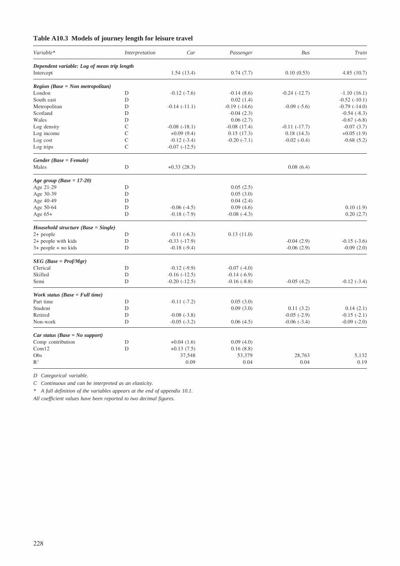
228

Table A10.3 Models of journey length for leisure travel


Dependent variable: Log of mean trip lengthIntercept 1.54 (13.4) 0.74 (7.7) 0.10 (0.53) 4.85 (10.7)

Region (Base = Non metropolitan)London D -0.12 (-7.6) -0.14 (8.6) -0.24 (-12.7) -1.10 (16.1)South east D 0.02 (1.4) -0.52 (-10.1)Metropolitan D -0.14 (-11.1) -0.19 (-14.6) -0.09 (-5.6) -0.79 (-14.0)Scotland D -0.04 (2.3) -0.54 (-8.3)Wales D 0.06 (2.7) -0.67 (-6.8)Log density C -0.08 (-18.1) -0.08 (17.4) -0.11 (-17.7) -0.07 (3.7)Log income C +0.09 (9.4) 0.15 (17.3) 0.18 (14.3) +0.05 (1.9)Log cost C -0.12 (-3.4) -0.20 (-7.1) -0.02 (-0.4) -0.68 (5.2)Log trips C -0.07 (-12.5)

Gender (Base = Female)Males D +0.33 (28.3) 0.08 (6.4)

Age group (Base = 17-20)Age 21-29 D 0.05 (2.5)Age 30-39 D 0.05 (3.0)Age 40-49 D 0.04 (2.4)Age 50-64 D -0.06 (-4.5) 0.09 (4.6) 0.10 (1.9)Age 65+ D -0.18 (-7.9) -0.08 (-4.3) 0.20 (2.7)

Household structure (Base = Single)2+ people D -0.11 (-6.3) 0.13 (11.0)2+ people with kids D -0.33 (-17.9) -0.04 (2.9) -0.15 (-3.6)3+ people + no kids D -0.18 (-9.4) -0.06 (2.9) -0.09 (2.0)

SEG (Base = Prof/Mgr)Clerical D -0.12 (-9.9) -0.07 (-4.0)Skilled D -0.16 (-12.5) -0.14 (-6.9)Semi D -0.20 (-12.5) -0.16 (-8.8) -0.05 (4.2) -0.12 (-3.4)

Work status (Base = Full time)Part time D -0.11 (-7.2) 0.05 (3.0)Student D 0.09 (3.0) 0.11 (3.2) 0.14 (2.1)Retired D -0.08 (-3.8) -0.05 (-2.9) -0.15 (-2.1)Non-work D -0.05 (-3.2) 0.06 (4.5) -0.06 (-3.4) -0.09 (-2.0)

Car status (Base = No support)Comp contribution D +0.04 (1.6) 0.09 (4.0)Com12 D +0.13 (7.5) 0.16 (8.8)Obs 37,548 53,379 28,763 5,132R2 0.09 0.04 0.04 0.19





229

Table A10.4 Stripped down models of journey length for business travel


Dependent variable: Log of mean trip lengthIntercept -0.48 (-1.9) +0.20 (0.4) -1.55 (-2.2) +1.30 (1.5)

Region (Base = Non metropolitan)London D -0.31 (-7.1) -0.45 (-5.4) -1.73 (-18.3)Metropolitan D -0.12 (-3.5)Scotland D -0.76 (-4.1)Log density C -0.03 (-2.9) -0.06 (-2.6) -0.12 (-3.1)Log income C +0.27 (10.9) +0.19 (3.8) +0.35 (5.2) +0.23 (2.7)

Work location (Base = Rural)London central D -0.31 (-7.1)Conurb central D -1.06 (-3.8)Urban outer D -0.29 (-10.7)Obs 9,858 2,613 999 904R2 0.03 0.00 0.07 0.29





Table A10.5 Stripped down models of journey length for commuter travel


Dependent variable: Log of mean trip lengthIntercept -1.06 (7.0) -0.03 (-0.1) +0.28 (1.19) +1.89 (5.5)

Region (Base = Non metropolitan)London D -0.14 (4.9) -0.17 (-4.3) -1.11 (-30.7)South east D +0.13 (7.1)Metropolitan D -0.49 (-6.9)Scotland D -0.59 (-7.4)Log density C -0.08 (-11.3) -0.07 (-4.5) -0.11 (-7.1)Log income C +0.31 (20.7) +0.17 (5.1) +0.14 (6.0) +0.11 (3.4)

Work location (Base = Rural)London central D +0.33 (5.5) +0.49 (3.5) +0.24 (3.8)Conurb central D +0.36 (5.3) +0.47 (3.5) 0.39 (7.1) -0.28 (-3.2)Urban central D -0.21 (-10.4) -0.16 (-4.0) -0.15 (-5.7) -0.25 (-4.5)Urban outer D -0.11 (-6.6) -0.37 (-5.6)Obs 19,472 3,332 3,790 1,935R2 0.04 0.03 0.05 0.34

D Categorical variable.C Continuous and can be inferred as an elasticity* A full definition of the variables appears at the end of appendix 10.1.All coefficient values have been reported to two decimal figures.

230

Table A10.6 Stripped down models of journey length for leisure passengers


Dependent variable: Log of mean trip lengthIntercept +0.82 (9.7) +1.0 (5.5) -0.12 (-1.2) +4.54 (10.3)

Region (Base = Non Metropolitan)London D -0.11 (-7.0) -0.163 (-10.2) -0.23 (-13.3) -1.12 (-16.1)South east D -0.53 (-10.2)Metropolitan D -0.13 (-10.2) -0.21 (-17.2) -0.09 (-6.4) -0.80 (-14.2)Scotland D -0.07 (-4.2) -0.56 (-8.7)Wales D -0.71 (-7.2)Log density C -0.08 (-18.1) -0.08 (-17.7) -0.11 (-17.8) -0.05 (-2.6)Log income C +0.13 (15.6) +0.19 (24.1) +0.19 (18.1) +0.05 (2.0)Log cost C -0.66 (-5.2) -0.63 (-7.8)Log trips C -0.08 (-14.6)Obs 37,548 53,379 28,763 5,132R2 0.03 0.03 0.03 0.18

D Categorical variable.C Continuous and can be interpreted as an elasticity.* A full definition of the variables appears at the end of appendix 10.1.All coefficient values have been reported to two decimal figures.

Table A10.7 NTS modelling outputs defined

Variable Description Variable Description

Region (Base = Non metropolitan) Household structure Base = SingleLondon London 2+ people 2 adults + no kids householdSouth east South east 3+ people with kids 3 adults + kids householdMetropolitan Metropolitan area 3+ people no kids 3 adults + no kids householdScotland Scotland Work status Base = Full timeWales Wales Part time Part time workerDensity Urban population density (persons per hectare) Student StudentLog density Density logged Retired RetiredIncome Personal income (£s) – 1997 Prices Non-work Not workingLog income Income logged Some maleCost Cost per trip (£s)- 1997 Prices Gender interaction Base = Male 17-20Log cost Cost logged Male age 30-39 Male aged 30-39Work place Base = Same Male age 40-49 Male aged 40-49Diff Work in diff locations Male age 50-64 Male aged 50-64Work location Base = Rural Car availability Base = No CarLondon central Central London All car Everyone has a car availableLondon outer Outer London Some male Some males have a car availableConurb central Non-London central conurbations Car status Base = No supportConurb outer Non-London outer conurbations Comp. contribution Employer contributes some of the cost of a car.Urban central Non-London central urban areas No free fuel Company car but no free fuelUrban outer Non-London outer urban areas Used for work Company car for work purposes onlyGender Base = Female Comp12 Company car for work with and without free fuelMale Male Free Fuel Company car with free fuelAge group Base = 17-20 SEG Base = Prof/MgrAge 21-29 Aged 21-29 Semi Semi skilled workerAge 30-39 Aged 30-39 Other Other type of workerAge 40-49 Aged 40-49 Clerical Clerical workerAge 50-64 Aged 50-64 Skilled Skilled worker

231

Table A10.8 Re-estimated car availability model

Standard logit

ASC-available +0.56 (1.5)Income (£s – 1997 prices) +0.00003 (26.1)Distance (miles) 0.04 (20.1)Car purchase cost index -0.02 (4.8)

Region (Base = Non met and Wales)London +0.20 (2.9)South east +0.15 (3.9)Metropolitan -0.20 (-5.4)Scotland -0.48 (-10.3)

Gender (Base = Female)Male +0.60 (18.4)Age (Base = 17-20)Age 21-29 +1.47 (27.2)Age 30-39 +1.78 (32.9)Age 40-49 +1.68 (31.0)Age 50+ +1.46 (26.8)

SEG (Base = Professional)Clerical -0.57 (-13.9)Skilled -0.62 (-13.7)Other -1.41 (-29.7)Workplace (Base = Same)Different places +0.69 (12.3)

Work location (Base = Rural, conurbation outer and urban outer)London central -1.42 (-18.3)London outer -0.37 (-4.8)Conurbation centre -0.61 (-6.0)Urban centre -0.31 (-9.4)

Public transport access (minutes)Bus 0.02 (7.9)Train 0.01 (9.4)

Bus frequency (Base = Less than hourly)At least hourly -0.34 (-7.1)At least half hourly -0.46 (-11.1)At least quarter hourly -0.77 (-17.7)

Multiple household workers (Base = Single worker household)Multi-household* +0.22 (+9.3)Multi-not household** -0.75 (-39.4)Obs 37,376r2 0.25

* Head of the household in a multi-worker household.

** Not the head of the household in a multi-worker household.

Table A10.12 defines the coefficients.

All variables relate to utility of car availability.

Re-estimated car availability model

In this section we present the re-estimated car availability model based upon the original car availability model that wasestimated by Wardman and Preston (2001).The choice set of whether a car is available for the journey to work is analysedusing a logit model fitted to NTS data from 1985 through to 1997. The key difference between the two models is that in there-estimated model the time trend terms have been removed.

232

Commuting mode choice

In Table A10.9 a multinomial logit model is presented which indicates the relative importance of different variables onmode choice for the journey to work. The model has been fitted to NTS data from 1985 through to 1997 and is a re-estimation of a model estimated by Wardman and Preston (2001).

Table A10.9 Car, passenger, bus and train mode choice model for the journey to work

Bus frequency (Base < 60mins)Freq 1 0.64 (5.9)Freq 2 1.08 (11.4)Freq 3 1.43 (14.9)

Access to PT (minutes)Walk - bus -0.02 (3.2)Walk - rail -0.04 (13.5)

Mode constants (Base = Car)Pass -3.74 (21.8)Bus -3.90 (19.2)Rail -3.88 (20.4)

Table A10.12 defines the coefficients.

Obs 32,623

Household structure (Base = Single)2 - Pass 0.34 (2.2)2 - bus -0.65 (4.7)2 - rail -0.42 (2.9)3 + C - pass 0.30 (1.9)3 + C - bus -0.80 (5.7)3 + C - rail -0.74 (5.2)3 + NC - pass 0.44 (2.7)3 + NC - bus -0.52 (3.6)3 + NC - rail -0.36 (2.3)

Multi household workers (Base = No)Multi - bus 0.31 (5.8)Multi - rail 0.32 (3.8)

Personal income (£s – 1997 prices)Income - bus -0.26 (6.3)Income - rail 0.00002 (4.9)Cost - car (£s) -0.004 (3.8)Cost - pass (£s) -0.01 (3.2)Cost - bus (£s) -0.002 (6.5)Cost - rail (£s) -0.002 (3.8)

SEG (Base = Prof/Mgr)Clerical - bus 0.34 (5.0)Skilled - pass 0.26 (3.5)Skilled - rail -0.69 (7.0)Other - pass 0.41 (3.6)Other - bus 0.36 (2.9)Other - rail -0.75 (5.0)

Car status (Base = No support)Comp car free fuel 1.11 (6.3)Comp car no free fuel 0.78 (4.6)Comp contribution 0.77 (4.4)Used for work 0.66 (5.4)

No car availableNo car - pass -0.36 (4.3)No car - rail -0.99 (10.3)

Work location (Base = Rural)Lon - central - pass 0.87 (4.8)Lon - central - bus 2.33 (16.9)Lon - central - rail 3.53 (29.5)Lon - outer - bus 0.84 (7.3)Lon - outer - rail 0.52 (4.2)Con - central - pass 0.97 (4.8)Con - central - bus 2.22 (12.4)Con - central - rail 2.83 (15.8)Con - outer - pass -0.42 (4.1)Urb - central - bus 0.69 (10.2)Urb - outer - pass -0.34 (3.8)Urb - outer - bus -0.19 (1.9)Urb - outer - rail -0.99 (8.1)

Gender PT access interaction (minutes)Walk - PT - male 0.008 (2.4)

Gender (Base = Female)Male - railρ2 0.52

Age group (Base = 17-20)Age 21-29 - passAge 21-29 - bus -0.36 (-4.5)Age 30-39 - pass -0.44 (4.3)Age 30-39 - bus -0.71 (5.9)Age 30-39 - rail -0.45 (4.3)Age 40-49 - pass -0.54 (4.7)Age 40-49 - bus -0.88 (7.3)Age 40-49 - rail -1.10 (8.1)Age 50+ - bus -0.81 (6.6)Age 50+ - rail -1.15 (8.2)Age 50+ - pass -0.33 (2.8)

Gender age interactionsMale 21-39 - pass -0.45 (4.9)Male 21-39 - bus -0.28 (3.0)Male 40+ - pass -0.47 (5.5)Male 40+ - rail 0.56 (4.3)

Pop density (persons per hectare)Dens - bus 0.002 (3.2)

Region (Base = Non metropolitan)London - pass -0.37 (3.7)London - rail 1.46 (11.6)SE - bus -0.15 (2.1)SE - train 1.18 (11.3)Met - pass -0.30 (5.2)Wales - rail 0.58 (2.7)Scot - rail 0.47 (3.6)

Work status (Base = Full time)Part time - pass -0.20 (3.2)Part time - rail -0.20 (1.8)

233

Table A10.10 Making or not making a trip by public transport

Variable EB* – rail EB - bus Leisure - rail Leisure – bus

Dependent Log public Log public Log public Log publicvariable transport trip transport trip transport trip transport trip

ASC-bustri -5.57 (-21.3) -4.48 (-34.1) -1.56 (-14.0) -0.06 (-0.9)

Gender (Base = Female)Male +0.61 (+7.7) -0.05 (-1.3) -0.52 (-23.8)

Age group (Base = 17-20)Age 3 +0.71(+3.4) -0.15 (-2.2) -0.71 (-17.0)Age 4 +0.69 (+3.4) -0.47 (-6.5) -1.04 (-24.2)Age 5 0.51 (+2.4) -0.14 (-2.0) -0.64 (-8.6) -1.05 (-24.3)Age 6 +0.19 (+0.9) -0.47 (-6.1) -0.88 (-11.5) -1.16 (-26.2)Age 7 -1.67 (-5.2) -2.7 (-12.2) -1.05 (-11.5) -1.34 (-27.0)Income (£s) 1997 prices +0.000038 (+13.3) +0.000032 (+2.4) +0.000021 (+12.9)Dens +0.0007 (+1.3) +0.001 (+5.1)

Region (Base = Non metropolitan)London +1.84 (+18.5) +1.04 (+11.2) +1.52 (+28.8) +0.41 (+12.5)South east +1.10 (+11.7) +0.30 (+3.3) +0.75 (+14.1) -0.15 (-5.5)Wales -0.68 (-1.9) -0.57 (-2.5)Scotland +0.56 (+5.3) +0.44 (+6.4) +0.37 (+11.7)Metropolitan +0.35 (+6.1) +0.45 (+18.2)

Access to PT (minutes)Walk bus +0.021 (+3.4) +0.0042 (+0.7) +0.007 (+1.7) -0.03 (-12.4)Walk train -0.01 (-4.0) -0.0041 (-2.1) -0.03 (-24.2) 0.005 (+7.9)

SEG (Base = No support)Cler -0.65 (-7.7) -0.55 (-8.3) -0.08 (-1.6) +0.24 (+8.0)Skill -1.33 (-11.4) -1.16 (-11.7) -0.74 (-12.1) +0.12 (+3.6)Semi -3.13 (-10.1) -1.44 (-12.7) -0.59 (-9.7) +0.22 (+6.8)

Work status (Base = Full time)Student +0.98 (+11.1) +0.32 (+4.9)Part +0.09 (+1.4) +0.36 (+11.3)Non work +0.15 (+2.8) +0.46 (+16.4)Retired +0.19 (+2.7) +0.73 (+21.9)

Household structure (Base = Single)2+ NC -0.15 (-3.7) -0.14 (-6.3)2+ C -0.58 (-12.2) -0.32 (-12.0)

Bus frequency (Base <60 mins)Freq 1 +0.56 (+15.1)Freq 2 +0.83 (+25.6)Freq 3 +1.10 (+32.6)

Car availability (Base = No car)Car 1 -0.37 (-3.5) -0.62 (-8.3) -0.36 (-17.2) -1.18 (-54.8)Car 2 -0.62 (-5.5) -1.07 (-12.0) -0.58 (-21.0) -1.67 (-61.2)Obs 921 1,346 5,135 28,841R2 0.22 0.11 0.16 0.17

* Employers business.

Table 10.12 defines the doefficients.

All variables relate to utility of making a trip.

Table A10.10 presents logit models that determine whether or not a person makes a specific trip or not. The modelshave been fitted to NTS data for the period 1985-1997 and cover employer business and leisure trips made by rail and bus.

234

Table A10.11 outlines the regression results from a model that has estimated the number of trips made by rail and bus onemployers business and for leisure trips given that the passenger chooses to travel by those modes for those purposes.

Table A10.11 Trip making if a person makes a trip by public transport

Variable EB – rail EB - bus Leisure - rail Leisure – bus

Dependent Log EB Log EB Log leisure Log leisurevariable rail trips bus trips rail trips bus trips

Intercept 0.86 (1.5) 0.59 (1.55) 0.00 (0.00) 1.00 (10.07)Log dens 0.04 (1.90) 0.02 (4.20)Log income (£s)1997 prices 0.01 (0.18) -0.02 (0.46) 0.10 (5.43) -0.05 (4.72)

Access to PT (minutes)Log walk bus -0.05 (6.55)Log walk train -0.07 (5.83) 0.06 (8.96)

Bus frequency (Base <60 mins)Freq 1 0.11 (5.6)Freq 2 0.19 (11.30)Freq 3 0.26 (14.92)

Region (Base = Non metropolitan)Scotland -0.26 (2.35) -0.09 (2.96) 0.16 (12.00)Metropolitan 0.21 (20.46)South east 0.15 (6.36)Lonondon 0.18 (8.08) 0.16 (11.37)

Gender (Base = Female)Male 0.11 (2.21) -0.05 (5.31)

Age group (Base = 17-20)Age 3 -0.06 (4.01)Age 4 0.13 (1.82) -0.09 (5.71)Age 5 -0.08 (4.94)Age 6 -0.10 (3.82) -0.08 (4.77)Age 7 -0.10 (2.61) -0.05 (2.61Age 23 0.05 (0.92)

Household structure (Base = Single)2+ NC -0.07 (6.44)2+ C -0.12 (9.76)Logcost (£s) -0.23 (1.61) 0.16 (6.17)

Work status (Base = Full time)Part 0.14 (8.76)Retired 0.19 (4.97) 0.38 (21.79)Non work 0.12 (4.79) 0.29 (21.35)

Number of cars in household (Base = No Car)Veh 1 -0.04 (0.79) -0.09 (4.51) -0.27 (27.32)Veh 2 -0.05 (0.82) -0.12 (4.56) -0.34 (23.92)

SEG (Base = Prof/Mgr)Skill 0.10 (1.74)Semi 0.16 (2.54)Semi-cler -0.08 (1.59)

Work place (Base = same)Diff 0.37 (5.26) 0.34 (5.65)Obs 921 1,346 5,135 28,841R2 0.06 0.04 0.06 0.18

Table A10.12 defines the doefficients.

235

Table A10.12 Definition of coefficients

Coefficient Description

Walk - bus (minutes) Access walk time for bus passengerWalk - rail (minutes) Access walk time for rail passenger

Gender PT access interactionAccess walk time for male passenger

Work location (Base = Rural)Lon - central - pass Central London + car passengerLon - central - bus Central London + bus passengerLon - central - rail Central London + rail passengerLon - outer - bus Outer London + bus passengerLon - outer - rail Outer London + rail passengerCon - central - pass Central conurbations + car passengerCon - central - bus Central conurbations + bus passengerCon - central - rail Central conurbations + rail passengerCon - outer - pass Outer conurbations + car passengerUrb - central - bus Central urban + bus passengerUrb - central - rail Central urban + rail passengerUrb - outer - pass Outer urban + car passengerUrb - outer - bus Outer urban + bus passengerUrb - outer - rail Outer urban + rail passenger

Number of car available (Base = No car)Car 1 1 car availableCar 2 2 cars availableNo car - pass No car available car passengerNo car - rail No car available rail passenger

Car status (Base = No support)Comp car free fuel Company car + free fuelComp car no free fuel Company car + no free fuelComp contribution Company contribution to car costUsed for work Company car for work journeys only

SEG (Base = Prof/Mgr)Clerical - bus Clerical worker + bus passengerSkilled - pass Skilled worker + car passengerSkilled - rail Skilled worker + rail passengerOther - pass Other type of worker + car passengerOther - bus Other type of worker + bus passengerOther - rail Other type of worker + rail passenger

Personal income and costs (£s – 1997 prices)Income Personal incomeIncome - bus Personal income of bus passengerIncome - rail Personal income of rail passengerCost - car Cost of travel for car ownerCost - pass Cost of travel for car passengerCost - bus Cost of travel for bus passenger


Pass Car passengerBus Bus passengerRail Rail Passenger

Distance to work (Miles) Walk - PT - male (minutes)Dist - pass For car passengerDist - rail For bus passenger

Region (Base = Non metropolitan)Lon LondonLondon - pass For car passengerLondon - bus For bus passengerLondon - rail For rail passengerSE - bus For south east bus passengerSE - train For south east train passengerMet MetropolitanMet - pass For metropolitan car passengerMet - rail For metropolitan car passengerWales WalesWales - rail For Welsh rail passengerScot ScotlandScot - rail For Scottish rail passenger

Time trendTrend - bus For bus passengerTrend - rail For rail passenger

Time trend and region interactionsTrend - Lon - bus For London bus passengerTrend - Lon - rail For London rail passengerTrend - SE - pass For SE car passengerTrend - SE - bus For SE bus passengerTrend - Wales - bus For Wales bus passengerTrend - Wales - rail For Wales rail passenger

Age group (Base = 17-20)Age 21-29 - pass Car passenger. aged 21-29Age 21-29 - bus Bus passenger. aged 21-29Age 30-39 - pass Car passenger. aged 30-39Age 30-39 - bus Bus passenger. aged 30-39Age 30-39 - rail Rail passenger. aged 30-39Age 40-49 - pass Car passenger. aged 40-49Age 40-49 - bus Bus passenger. aged 40-49Age 40-49 - rail Rail passenger. aged 40-49Age 50+ - bus Bus passenger. aged 50+Age 50+ - rail Rail passenger. aged 50+Age 50+ - pass Car passenger. aged 50+

Gender (Base = Female)Male MaleMale - rail Male rail passenger

Continued ....

236


Freq 1 Bus frequency greater than or equal to every 60 minutesFreq 2 Bus frequency greater than or equal to every 30 minutesFreq 3 Bus frequency greater than or equal to every 15 minutes

Multi household workers (Base = No)Multi - bus Belongs to a multi-worker household and is a bus passMulti - rail Belongs to a multi-worker household and is a rail pass

Household structure (Base = Single)2+ NC Belongs to a 2 adult household2+ C Belongs to a 2 person household (including a child)2 - pass Belongs to a 2 adult household and is a car passenger2 - bus Belongs to a 2 adult household and is a bus passenger2 - rail Belongs to a 2 adult household and is a rail passenger3+C - pass Belongs to a 3 or more person household (including a child) and is a car passenger3+C - bus Belongs to a 3 or more person household (including a child) and and is a bus passenger3+C - rail Belongs to a 3 or more person household (including a child) and is a rail passenger3+NC - pass Belongs to a 3 or more adult household and is a car passenger3+NC - bus Belongs to a 3 or more adult household and is a bus passenger3+NC - rail Belongs to a 3 or more adult household

Work status (Base = Full Time)Part Part time workerPart time - pass Part time worker who is a car passengerRetired RetiredNon work Not workingStudent StudentPart time - rail Part time worker who is a rail passenger

Work place (Base = Same)Diff Work in different locations

Pop density (persons per hectare)Dens Population densityDens - bus Population density of persons who are bus passengersDens - rail Population density of persons who are rail passengers

Gender age interactionsMale 21-39 - pass 21 to 39 yr old male who is a car passengerMale 21-39 - bus 21 to 39 yr old male who is a bus passengerMale 40+ - pass 40+ year old male who is a car passengerMale 40+ - rail 40+ year old male who is a rail passengerCost-rail Cost of rail

Household car ownership (Base = No car)Veh 1 1 Car householdVeh 2 2 Car household

237

Prices current at January 2004

For further details of these and all other TRL publications, telephone Publication Sales on 01344 770783, or visitTRL on the Internet at www.trl.co.uk.

Abstract

This document reports on the outcome of a collaborative study the objective of which was to produce an up-to-dateguidance manual on the factors affecting the demand for public transport for use by public transport operators andplanning authorities, and for academics and other researchers. The context of the study was principally that of urbansurface transport in Great Britain, but extensive use is made of international sources and examples. Analysis and researchby using primary and secondary data sources on the influencing factors were pursued to produce a document that assistsin identifying cost-effective schemes for improving services. A wide range of factors was examined. The study has re-examined the evidence from an earlier, 1980, study on the factors affecting the demand for public transport, and hasextended the coverage from that of the 1980 study to reflect the changing sociological and policy background.

Related publications

TRL419 Summary of the EUROTOLL project by M Ingrey and P Fouracre. 1999 (price £25, code E)

TRL410 Leeds guided busway study by G G Daugherty and R J Balcombe. 1999 (price £35, code J)

TRL409 A comparative assessment of major bus priority schemes in Great Britain by G G Daugherty,R J Balcombe and A J Astrop. 1999 (price £35, code J)

TRL399 Workplace parking levy by T Wang and J Sharples. 1999 (price £25, code E)

TRL366 Concessionary fares: trip generation among elederly passengers by R J Balcombe, A Astrop and E Hill.1998 (price £35, code H)

TRL330 Information for bus passsengers: a study of needs and priorities by R J Balcombe and C E Vance.1998 (price £35, code H)

TRL271 Evaluation of low-floor bus trials in London and North Tyneside by I York and R J Balcombe.1998 (price £35, code H)

TRL166 Responses to concessionary fare changes in Tyne and Wear by R J Balcombe and A Astrop.1995 (price £35, code H)

TRL142 Passenger reactions to present and alternative travelcard schemes by I York. 1995 (price £35, code H)

CR183 The scope for ridership growth on minibuses: the results of passenger surveys by R P Turner, P R White,K Hoogendam and P F Watts. 1990 (price £25, code E)

RR291 An analysis of concessionary bus fare schemes for OAPs using the 1985/86 National Travel Survey byD O’Reilly. 1990 (price £20, code B)

RR127 Bus trip generation from concessionary fare schemes: a study of six towns by P B Goodwin, J Hopkin,and R McKenzie. 1988 (price £20)

RR69 Concessionary fares and pensioners’ travel patterns: an analysis based on the 1978/9 National TravelSurvey by J Hopkin. 1986 (price £20)

SR825 The effect of the Tyne and Wear metro on residential property values by M W Pickett and K E Perrett.1984 (price £20)

SR821 The impact of transport policy on the city by R L Mackett. 1984 (price £20)

SR800 The Glasgow rail impact study: summary report by H Gentlemen, C G B Mitchell, Walmsley, D A andWicks, J. 1983 (price £20)

SR338 The effect of free public transport on the journey to work by A J Daly and S Zachery. 1977 (price £20)

SR614 Fares elasticity of suburban rail travel by P Hughes. 1980 (price £20)

LR993 The elasticity for medium distance rail travel by R Oldfield and E Tyler. 1981 (price £20)

LR991 Benefits and costs of providing additional information about urban public transport services by P Ellsonand R Tebb. 1981 (price £20)

LR872 Effect of car ownership on bus patronage by R Oldfield. 1979 (price £20)

LR825 Cost and benefit of a bus-service information leaflet by P Ellson and R Tebb. 1978 (price £20)

LR733 The effect of fares on bus patronage by P H Bly. 1976 (price £20)

LR699 Depleted bus services: the effect of rescheduling by P H Bly. 1976 (price £20)

CT135.1 Transport demand and modal shift update (1999-2002) Current Topics in Transport: selected anstractsform TRL Library’s database (price £20)

The demand for public transport: a practical guide · Steve Lowe (MVA) Roland Niblett (Colin...

Documents

Transcript of The demand for public transport: a practical guide · Steve Lowe (MVA) Roland Niblett (Colin...