The Dawes Review 1: Kinematic studies of star-forming ...richard/ASTRO620/kinematics_galaxies... ·...

The Dawes Review 1: Kinematic studiesof star-forming galaxies across cosmictime

Karl Glazebrook A,B

A Centre for Astrophysics and Supercomputing, Swinburne University of Technology, P.O. Box 218,

Hawthorn, VIC 3122, AustraliaB [email protected]

Updated 9/Jun/2014. Published as PASA, 30, e056 (2013). doi:10.1017/pasa.2013.34. A few minorcorrections have been made to the journal version.

Abstract: The last seven years have seen an explosion in the number of Integral Field galaxy surveys,obtaining resolved 2D spectroscopy, especially at high-redshift. These have taken advantage of themature capabilities of 8–10m class telescopes and the development of associated technology such asAO. Surveys have leveraged both high spectroscopic resolution enabling internal velocity measurementsand high spatial resolution from AO techniques and sites with excellent natural seeing. For the firsttime we have been able to glimpse the kinematic state of matter in young, assembling star-forminggalaxies and learn detailed astrophysical information about the physical processes and compare theirkinematic scaling relations with those in the local Universe. Observers have measured disc galaxyrotation, merger signatures and turbulence-enhanced velocity dispersions of gas-rich discs. Theoristshave interpreted kinematic signatures of galaxies in a variety of ways (rotation, merging, outflows, andfeedback) and attempted to discuss evolution vs theoretical models and relate it to the evolution ingalaxy morphology. A key point that has emerged from this activity is that substantial fractions ofhigh-redshift galaxies have regular kinematic morphologies despite irregular photometric morphologiesand this is likely due to the presence of a large number of highly gas-rich discs. There has not yet been areview of this burgeoning topic. In this first Dawes review I will discuss the extensive kinematic surveysthat have been done and the physical models that have arisen for young galaxies at high-redshift.

Keywords: galaxies: evolution, galaxies: formation, galaxies: high-redshift, galaxies: kinematics anddynamics, galaxies: stellar content, galaxies: structure

The Dawes Reviews are substantial reviews of topical ar-eas in astronomy, published by authors of internationalstanding at the invitation of the PASA Editorial Board.The reviews recognise William Dawes (1762–1836) (pic-tured in Figure 1), second lieutenant in the Royal Marinesand the astronomer on the First Fleet. Dawes was notonly an accomplished astronomer, but spoke five lan-guages, had a keen interest in botany, mineralogy, engi-neering, cartography and music, compiled the first Abor-iginal-English dictionary, and was an outspoken opponentof slavery.

‘Eppur si muove’

– Galileo Galilei (apocryphal)

1 Introduction

The advent of new large telescopes coupled with newinstrumentation technologies in the last decade has

been extremely powerful in expanding our view of thehigh-redshift Universe. In particular, we have seen aflowering of the topic of high-redshift galaxy kinemat-ics which studies their internal motions through highspatial and spectral resolution observations. The num-ber of papers has exploded and we have seen a varietyof surveys of observational approaches, analysis tech-niques, and theoretical interpretations. This has led tonew paradigms of the nature of young galaxies but ithas also raised problems in understanding as many newtechniques have been used making comparison withthe local Universe and traditional techniques difficult.

The Publications of the Astronomical Society ofAustralia has decided to launch this new series of ma-jor reviews in honour of Lt. William Dawes. I havechosen to write it on the topic of these exciting newstudies of the kinematics of high-redshift star-forminggalaxies, one which has not had a major review andis in need of one. This is the first such Dawes reviewand as such there is no tradition to follow, instead onegets to set the tradition. I will choose to write this asa high-level introduction to the field, perhaps akin to

1

arX

iv:1

305.

2469

v4 [

astr

o-ph

.CO

] 9

Jun

201

4

http://adsabs.harvard.edu/cgi-bin/nph-abs_connect?fforward=http://dx.doi.org/10.1017/pasa.2013.34

2 Publications of the Astronomical Society of Australia

the style of lecture notes, for the new worker in thefield (for example an incoming postgraduate student).As such I will try and favour clarity and simplicity ofexplanations over totally complete lists of all possiblereferences and ideas on a topic and will discuss analy-sis techniques in some detail. I will highlight the mainsurveys and the main ideas and warn in advance thatsome things may get left out. I will also allow myselfthe freedom to give more scientific speculation of myown than would occur in a traditional review, howeverit will be clearly indicated what is a speculation. Ob-viously I will use the first person when needed as thisseems appropriate for my approach.

1.1 Background and scope of this review

The rotation of the ‘spiral nebulae’ was one of the ear-liest and most fundamental observations of their na-ture and the second important discovery from theirspectroscopy. Almost exactly 100 years ago in 1912September, Vesto M Slipher measured the first spec-trum and first redshift of a galaxy using a new fastspectrograph he had built (Slipher 1913). This galaxywas M31 and the redshift was actually a blueshift of300 km/s — this was highly unexpected at the time,it was ten times higher than any previous velocitymeasured for an astronomical object. Slipher himselfthought it good evidence for the extragalactic modelof spiral nebulae (Bartusiak 2009) and proceeded toembark on a campaign to measure many more veloc-ities (Slipher 1917) eventually resulting in one axis ofHubble’s famous diagram (Hubble 1929).

Less well-known is that during this first campaignSlipher also discovered the rotation of galaxies (Slipher1914) — he noticed the tilt of the spectral lines whilstobserving the Sa galaxy M104 and noted the similar-ity to the same phenomenon when observing planets.Slipher had worked for Lowell for many years measur-ing the day lengths of various planets. Slipher com-mented: ‘Although from the time of Laplace it has beenthought that nebulae rotate, this actual observation ofthe rotation is almost as unexpected as was the discov-ery that they possessed enormously high radial veloci-ties’.

We now regard galaxies as gravitationally boundextragalactic objects and their internal motions relateto fundamental questions about their masses and as-sembly history. In particular the last seven years haveseen a wealth of new high-redshift observations mea-suring for the first time the kinematics of galaxies inthe early Universe and producing new pictures of star-forming galaxies. These are the topic for this review.I note that I will favour the term ‘kinematics’ whichdescribes, from observations, the motions of astronom-ical objects (as opposed to the term ‘dynamics’ whichdescribes the theoretical causes of such motions).

Large 8-10m class optical telescopes1 with their

1The overwhelming majority of kinematic observationsat z > 0.5 have been optical/near-infrared utilising nebulaemission lines, however radio/sub-mm observations will bementioned and this balance is likely to change dramaticallyin the next decade with the advent of the Atacama LargeMillimetre Array (ALMA).

Figure 1: William Dawes was a Royal Marine offi-cer on the ‘First Fleet’ arriving in Australia in 1788.He was a man of many talents: engineer, map maker,botanist, and amateur astronomer. He was one of thefirst to document the Aboriginal Australian languagesspoken in the Sydney region. He was the first personto make astronomical observations in Australia usingtelescopes from a place in Sydney Cove now knownas Dawes Point (Mander-Jones 1966). Image Credit:miniature oil painting of Lieutenant William Dawes,1830s, artist unknown. Collection: Tasmanian Mu-seum and Art Gallery. Reproduced with their permis-sion.

light grasp and angular resolution have been critical forthe development of this subject but equally importanthas been the associated development of astronomicalinstrumentation sitting at the focal plane.

Integral Field Spectroscopy (IFS) has played a piv-otal role due to the complex structures of high-redshiftobjects. With this technique, it is possible to collecta spectrum of every point in the 2D image of an ob-ject, which is contrasted with the classical technique oflong-slit spectroscopy where spectra are collected alonga 1D slice (whose direction must be chosen in advance)through an object. An IFS generally works by refor-matting a 2D focal plane, and there are various waysof accomplishing this (for a review of the technology,see Allington-Smith (2006)) but a general principle isthat because instruments are limited by the number ofpixels in their focal plane detectors, an IFS typicallyhas a small field of view with spatial sampling of order1000 elements2 suitable for single object work. (This

2IFS spatial sampling elements (e.g. lenslets or fibres)

http://www.tmag.tas.gov.au

http://www.tmag.tas.gov.au

K. Glazebrook 3

is an area that is likely to improve in the future withnew instruments and ever large pixel-count detectors).

Adaptive Optics (AO) technology which correctsfor atmospherical turbulent blurring of images has alsobecome routine on large telescopes (Davies & Kasper2012) over the last decade and has allowed the achieve-ment of the angular diffraction limit on 8-10m tele-scopes — typically 0.1 arcsec instead of the 0.5–1 arc-sec seeing limit imposed by the atmosphere. This is im-portant as 1 arcsec corresponds to 8 kpc for 1 < z < 3which is comparable to the sizes of disc galaxies atthese redshifts (e.g. Ferguson et al. (2004); Buitragoet al. (2008); Mosleh et al. (2011)). AO observingcomes with its own sets of limitations imposed by therequirements to have bright stars or laser beacons tomeasure AO corrections from and have generally notbeen possible for all objects in large samples.

It is important when writing a review to carefullydefine the scope. The topic will be the kinematics ofstar-forming galaxies at high-redshift (which I will de-fine as z > 0.5), with a focus on what we have learnedand how we have learned it, from IFS and AO ob-servations. It is not possible to cover, with any com-prehensiveness related topics such as (i) general phys-ical properties of high-redshift star-forming galaxies,(ii) the kinematics of star-forming galaxies in the localUniverse, and (iii) the kinematics of non-star form-ing ‘red and quiescent’ galaxies at high-redshift. Thefirst two are already the subject of extensive reviewsto which I will refer, and the last is a rapidly burgeon-ing field which will probably be due for its own reviewin 2–3 years as the number of observations increasestremendously with the advent of multi-object near-IR spectrographs.3 However, some non-comprehensivediscussion of each of these (especially the first two) willbe given to set the scene.

The plan and structure of this review is as fol-lows. Firstly, in the remainder of this introductionI will briefly discuss the kinematic properties of galax-ies in the modern Universe to frame the comparisonswith high-redshift. In Section 2, I will review the earli-est kinematic observations of star-forming galaxies athigh-redshift from longslit techniques. In Section 3,I will review the most important large high-redshiftIFS surveys, how they are selected and carried outand their most important conclusions. In Section 4,I will review the kinematic analysis techniques usedby IFS surveys with reference to the surveys in Sec-tion 3. In Section 5, I will compare and contrast whatwe are learning about the physical pictures of high-redshift star-forming galaxies from the various IFS sur-veys and discuss, in particular, the ‘turbulent clumpydisc’ paradigm that has arisen from these works. In

are often called ‘spaxels’. This I mention solely to recordfor posterity this great quote: ‘If spatial bins are spaxels,are spectral bins spexels and time bins tixels? But wait atixel, those spaxels and spexels are all pixels or voxels! Isay, purge the English language of these mongrel wordels!’(Matthew Colless, 2010, personal communication)

3I note that spatially resolved kinematic observationsof red galaxies at high-redshift will prove very difficult asit would require the detection and measurement of stellarabsorption lines at even higher angular resolution in smallerobjects than has been done for the star-forming population.

Section 6, I will point to the future, the outstandingquestions and the future instruments, telescopes, sur-veys and techniques that may address them.

This review will adopt a working cosmology of Ωm =0.3, ΩΛ = 0.7, H0 = 70 km s−1 Mpc−1 (Spergel et al.2003). Since most of the work discussed has been inthe last decade, the authors have adopted cosmologiesvery close to these resulting in negligible conversionfactors in physical quantities. I will adopt the use ofAB magnitudes.

1.2 Kinematics of star-forming galaxies inthe local Universe.

In the local Universe, we see a distinct separation ofgalaxies in to two types with red and blue colours(Strateva et al. 2001; Baldry et al. 2004) commonlyreferred to as the ‘red sequence’ and ‘blue cloud’ re-flecting the relative tightness of those colour distribu-tions. The separation is distinct in that there is aclear bimodality with a lack of galaxies at interme-diate colours. These colour classes are very stronglycorrelated with morphology either as determined visu-ally or via quantitative morphological parameters —a detailed recent review of these properties as derivedfrom large statistical surveys such as the Sloan Dig-ital Sky Survey and exploration of their dependenceon other parameters such as environment is given byBlanton & Moustakas (2009). The correlation is suffi-ciently strong that virtually every massive system onthe blue cloud is a rotating star-forming disc galaxy(usually spiral), though there is a rare population of‘red spirals‘ which overlap the red sequence (which ismostly ellipticals) that may arise from truncated star-formation, greater older stellar population contribu-tions or dust (Masters et al. 2010; Cortese 2012).

There has been a number of reviews on the topicof the kinematics of local disc galaxies over the years,which should be referred to for a comprehensive discus-sion. In this section, I will discuss the most importantpoints mostly referencing recent results whilst notingthat the subject has a long history which has been wellcovered elsewhere. I refer the reader for more depthand history to van der Kruit & Allen (1978), who re-view the kinematics of spiral and irregular galaxies andSofue & Rubin (2001), which is a more focussed reviewon the topic of rotation curves. A classic review of thestructure of the Milky Way in particular was done byGilmore et al. (1989). Recently van der Kruit & Free-man (2011) wrote a very comprehensive recent reviewof all properties of galaxy discs including kinematics.

For comparison with high-redshift, the most fun-damental properties of local star-forming galaxies aretheir rotation and velocity dispersion, whose most im-portant points I will review below. However, as wewill see later in this review, star-forming galaxies athigh-redshift show more kinematic diversity than inthe local Universe including high fractions which arenot dominated by rotation or which show complexkinematic signatures of mergers. Given evolutionarypaths from high-redshift to low-redshift and from star-forming to quiescent are not obvious I will also discussbriefly the kinematics of local elliptical galaxies and


mergers.

1.2.1 Rotation of local star forming galax-ies

The earliest published work on disc galaxy rotationwas that of Slipher (1914) but also see Pease (1916).They measured the rotation of several spirals between1914 and 1925 including M31 and M104. The reviewof Sofue & Rubin (2001) gives a historical introduc-tion, so also does the one of van der Kruit & Allen(1978). The early optical work was limited to the cen-tral regions of galaxies, the advent of radio telescopesand neutral hydrogen HI observations (van de Hulstet al. 1957; Argyle 1965) permitted measurements outat large radii where most of the angular momentumlies. Radio observations led to the well-known andmost fundamental scaling of disc galaxies: the ‘Tully-Fisher Relation’ first reported by Tully & Fisher (1977)between optical luminosity and HI line width. If theHI line width, from an unresolved or marginally re-solved single-dish observation, is thought of as tracingthe total kinematic shear, then this becomes a relationbetween luminosity and rotation velocity, and henceluminosity and a measure of mass. Later, Tully-Fisherwork has benefited from greatly increased spatial reso-lution and 2D kinematic mapping of the rotation field.

In the standard pictures, we now think of galaxiesas inhabiting haloes of Cold Dark Matter (CDM), anon-baryonic component that dominates the dynam-ics and sets the scene for galaxy formation (Blumen-thal et al. 1985; Ostriker 1993). The most funda-mental of observations supporting this picture is the‘flat rotation curves’ of disc galaxies (Rubin & Ford1970; Roberts & Rots 1973; Rubin et al. 1978). Thegeneral picture is of a steeply rising rotation curve inthe innermost few kpc followed by the ‘flat’ portion,which really means a turnover and then a slight slowdecline in more luminous galaxies or a flatter moreconstant rotation in lower luminosity galaxies (Persicet al. 1996; Sofue & Rubin 2001). This occurs in aregime where the optical surface brightness is exponen-tially dropping off and the rotation velocity, as tracedby HI, stays high past the outer edge of the opticaldisc. If light traced mass the velocity would drop offmore sharply, this is the basic evidence for dark mat-ter haloes (though is not universally accepted, for analternative paradigm involving ’Modified NewtonianDynamics’ see Sanders & McGaugh (2002)). If a darkmatter halo was spherical and isothermal (ρ ∝ r−2),one expects a perfectly flat rotation curve, in real-ity simulations predict more complex profiles for darkmatter haloes (Navarro et al. 1997) and this, togetherwith the stellar contributions, must be carefully con-sidered when fitting rotation curve models (Kent 1987;Blais-Ouellette et al. 2001)). As such when definingthe ‘rotation velocity’, one must be careful to specifyat what radius this is measured. A common conven-tion is to use 2.2 disc scalelengths4 (from the surfacephotometry) as this is the radius where the rotationcurve of a self-gravitating ideal exponential disc peaks

4It is useful to also note that 2.2 scalelengths is also 1.3×the half-light radius for a pure exponential disc.

(Freeman 1970a). This ‘v2.2’ can also be related tothe HI line width (Courteau 1997) which also probesthe outer rotation. The typical values for large discgalaxies are in the range 150–300 km/s.

The original Tully-Fisher relation displayed a slopeof L ∝ V 2.5 (based upon the luminosity from blue-sensitive photographic plates), modern determinationsfind an increasing slope with wavelength rising to aslope of V 4 in the K-band or with stellar mass (Bell &de Jong 2001; Verheijen 2001). This is consistent withgalaxies having a roughly constant ratio of dark mat-ter to stellar mass globally5 — which is in contrast tothe resolved distribution within galaxies where clearlyit does not. CDM theory predicts a slope closer toV 3 based on scaling of dark matter halo properties(Mo et al. 1998). Some authors have argued that thisrepresents an unreasonable ‘fine-tuning’ of the ΛCDMmodel and have proposed an alternative gravity ‘MOND’mode without dark matter (e.g. Sanders & McGaugh(2002); McGaugh & de Blok (1998); McGaugh (2012)),however small scatter can be accommodated withinthe ΛCDM framework (Gnedin et al. 2007; Avila-Reeseet al. 2008; Dutton 2012). MOND does not seem to ex-plain well larger scale structures such as galaxy groupsand clusters in the sense that even with MOND thereis still a need to invoke dark matter to explain the kine-matics (Angus et al. 2008; Natarajan & Zhao 2008).This review will only consider the ΛCDM cosmologicalframework.

1.2.2 Velocity dispersion of local galaxydiscs

We next consider the vertical structure and pressuresupport of galactic discs, as this will become quite asignificant topic when comparing with high-redshift,where we will see substantial differences. The mostobvious visible component of spiral galaxy discs is theso-called ‘thin disc’ which is where the young stel-lar populations dwell. The stellar component of thethin disc has an exponential scale height of 200–300 pcand a vertical velocity dispersion (σz) of ∼ 20 km s−1

(van der Kruit & Freeman 2011) — the dispersion isrelated to the vertical mass distribution by a gravita-tional equilibrium. This is σ2

z = aGΣhz where Σ isthe mass surface density, hz is the vertical exponen-tial scale height, and a is a structural constant = 3π/2for an exponential disc. In general, the dispersion ofa stellar disc is a 3D ellipsoid (σR, σθ, σz). The radial(σR) and azimuthal (σθ) components are related by theOort constants (giving σθ ' 0.71σR for a flat rotationcurve) and the radial and vertical components are re-lated to the discs structure and mass to light ratio witha typical value of σz/σR ∼ 0.6 for large spirals (againsee van der Kruit & Freeman and references thereinfor an extensive discussion of this).

The stellar age range of the Milky Way thin discis up to 10 Gyr. Right in the middle of the thin discis an even thinner layer where the gas collects — theneutral hydrogen, molecular clouds, dust, HII regions,

5i.e. if discs form a one parameter sequence of constantcentral surface brightness, then L ∝ r2 and with GM ∝rV 2 one can easily show that if M ∝ L then L ∝ V 4

K. Glazebrook 5

and young OB and A stars all sit in this thinner layerwhich has a dispersion of only ∼ 5–10 km s−1 and scaleheight of 50 pc in the Milky Way. This thinner discis where all of the star formation takes place todayand in which the characteristic spiral structure of gasand young stars is apparent. In our Milky Way, theyoungest stars (OBA spectral types) share the kine-matics of the gas disc in which they form, as stellarage increases the velocity dispersion also increases —this kinematic evolution is interpreted as being due tostars on their orbits encountering ‘lumps’ in the disc,and scattering off them, such as giant molecular clouds(GMC’s) and spiral arms. This gives rise to the thinstellar disc having on average a higher dispersion thanthe gas disc and young stars. The difference in velocitydispersion between different components gives rise tothe phenomenon known as ‘asymmetric drift’; for ex-ample, the rotation of the stellar disc lags behind thatof the gas disc due to it’s higher radial velocity dis-persion which provides additional dynamical supportagainst the galaxy’s overall gravitational field.

Many external galaxies have their gas and kinemat-ics observed in the Hα line of ionised hydrogen whoseluminosity is generally dominated by HII regions. Inthe Milky Way, HII regions and GMCs share the lowvelocity dispersion (i.e. between cloud centres, Stark& Brand (1989)) of the gas disc; however, it should benoted that the Hα line has a thermal broadening dueto a characteristic temperature of 104K of ∼ 9 km s−1

which will increase the observed line width. There isalso a turbulent broadening due to internal motionsin HII regions of order 20 km s−1 (Mezger & Hoglund1967; Shields 1990). Adding these in quadrature, wecan see the typical dispersion is consistent with therange of 20–25 km s−1 found by observations of exter-nal nearby spirals (Epinat et al. 2010; Andersen et al.2006a).

The Milky Way also has a a so-called ‘thick disc’stellar component (Gilmore & Reid 1983) (though thereis still a debate as to whether this is a true dichotomyor a continuous stellar population sequence, e.g. Bovyet al. (2012a,b).). Thick discs are now thought to beubiquitous in spirals and may have masses that are,on average, up to values comparable to the thin disc(Comeron et al. 2011). The thick discs contain older,redder, and lower surface brightness populations andnegligible on-going star-formation (Yoachim & Dalcan-ton 2008). The thick disc in our Milky Way has ascale height of ∼1400 pc (Gilmore & Reid 1983). It islow metallicity ∼ 1/4 Solar, is ∼ 10 Gyr old (Gilmoreet al. 1989) and has a vertical velocity dispersion of ∼40 km s−1 (Chiba & Beers 2000; Pasetto et al. 2012).Other spirals are thought to be similar. The origin ofthick discs is a matter of debate and there are a vari-ety of models — it may be formed from early mergerevents, satellite accretion, or secular evolution (see dis-cussion in van der Kruit & Freeman (2011) and refer-ences therein). A particularly relevant scenario for ourlater discussion is the idea that the thick discs form insitu in early gas-rich high-dispersion discs (Bournaudet al. 2009).

Figure 2 illustrates these components schematicallyand also contrasts them with the emerging (but by no

Stellar thin disk σz ~ 20 km/s, hz~200–300 pcStellar thick disk σz ~40 km/s, hz~1500 pc

HI gas, molecular gas, GMCs, HII regions, OBA starsσz ~ 5 km/s, hz~50 pc

(Note thermal 104K broadening of Hα ~ 9 km/s)

z~0

HI gas, molecular gas, sGMCs?, sgHII regions (~1–2 kpc), OBA starsσz ~ 50 km/s, hz~1500 pc

tadpole (97), spiral (269), and elliptical (100). Figure 1 shows

eight examples of each type; the lines correspond to 0B5.

Galaxy morphology can vary with wavelength, so we viewed

many of the cataloged objects at other ACS passbands and with

NICMOS (Thompson et al. 2005). Generally, the morphologi-

cal classification does not change significantly with wavelength

(e.g., Dickinson 2000) because it is based on only the most fun-

damental galaxy characteristics, such as elongation and number

of giant clumps. Also, the NICMOS images have a factor of 3

lower resolution, so they do not reveal the same fine structure as

the other images.The distinguishing characteristics of the main types that we

classified are as follows:

Chain.—Linear objects dominated by several giant clumps

and having no exponential light profiles or central red bulges.

Clump cluster.—Oval or circular objects resembling chain

galaxies in their dominance by several giant clumps and having

no exponential profiles or bulges.

Double clump.—Systems dominated by two similar clumps

with no exponential profile or bulge.

Tadpole.—Systems dominated by a single clump that is off-

center from, or at the end of, a more diffuse linear emission.

Spiral.—Galaxies with exponential-like disks, evident spiral

structure if they have low inclination, and usually a bulge or a

nucleus. Edge-on spirals have relatively flat emission from a mid-

plane, and often extended emission perpendicular to themidplane,

as well as a bulge.Elliptical.—Centrally concentrated oval galaxies with no

obvious spiral structure.

Chain galaxies were first recognized by Cowie et al. (1995)

using the same definition as that here. Tadpole galaxies were de-

fined by van den Bergh et al. (1996), and examples from the UDF

were discussed by Straughn et al. (2004). Tadpole galaxies with

short tails were classified as ‘‘comma’’ type in the morphology

review by van den Bergh (2002). Van den Bergh et al. (1996) also

noted objects like clump clusters and called them ‘‘protospirals.’’

Conselice et al. (2004) called these clump-dominated young disk

galaxies ‘‘luminous diffuse objects,’’ although some of their sam-

ple included galaxies with bulges and exponential-like profiles,

unlike the clump clusters here. Binary galaxies, like our doubles,

Fig. 1aFig. 1bFig. 1.—Selection of eight typical galaxies for each morphological type: four in (a) and four in (b). Top to bottom: Chain, clump-cluster, double, tadpole, spiral, and

elliptical galaxies. Images are at i775 band, with a line representing 0B5. UDF or our own identification numbers from left to right in (a) are as follows: chains: 6478, 7269,

6922, 3214; clump clusters: CC12, 1375, 2291, 5190; doubles: 637, 4072, 5098, 5251; tadpoles: 3058, 8614, 5358, 6891; spirals: 3372, 3180, 4438, 8275; ellipticals:

2107, 4389, 2322, 4913. In (b), the identifications are: chains: 169 and 170 (two separate galaxies), 1428, 401, 3458+3418; clump clusters: 6486, 4807, 7230, 9159;

doubles: 2461, 2558, 4097, 3967; tadpoles: 9543, 5115, 3147, 9348; spirals: 2607, 5805, 7556, 5670; ellipticals: 8, 4527, 4320, 5959. Panel b has an example of an

edge-on spiral.

Fig. 1a

Fig. 1b

ELMEGREEN ET AL.

86

Vol. 631

z~2

Figure 2: Illustrative schematic showing the differ-ent structures of low-redshift and high-redshift discgalaxies in an edge-on view. Top: components of theMilky Way and similar local spirals (see Section 1.2.2)containing stellar thin/thick discs and a very thin gasdisc in the centre. The latter contains all the GiantMolecular Clouds, HII regions, molecular and neutralgas and young stars. Bottom: a clumpy high-redshiftdisc (see Section 5.1). This contains a thick (∼ 1 kpcscaleheight) and highly turbulent discs of moleculargas, young stars, super-giant HII regions (kpc scalestar-forming ‘clumps’ ) and (presumably) super-GiantMolecular Clouds. Credit: inset images are of NGC4565 (top, reproduced by permission of R. Jay Ga-Bany, Cosmotography.com) and z ∼ 3 galaxy UDF#6478 of Elmegreen & Elmegreen (2006) (their Fig-ure 2, reproduced by permission of the AAS).

means certain) picture of z ∼ 2 galaxies which we willreturn to in Section 5.1.

In this review, I will use the words ‘velocity dis-persion’ frequently. First, I should note that what ismeasured from spectra is always ‘line-of-sight velocitydispersion’. Secondly, I note that in the literature it isused in two principal senses:

1. Resolved velocity dispersion (sometimes called‘intrinsic dispersion’ or ‘local dispersion’) by whichwe mean the dispersion as measured in line widthsof elements of spatially resolved observations. Agalaxy disc is a good physical example, in thiscase the dispersion refers to the random motionsof stars and gas around the mean rotation fieldat each position.

2. Integrated velocity dispersion by which we meanthe dispersion as measured from an integrated

http://cosmotography.com


spectrum (i.e. spatially averaged). In this case,this will include a (possibly dominant) contribu-tion from any global velocity field such as rota-tion. The HI line width used in the Tully-Fisherrelation is a classic example of this, as are thecentral ‘velocity dispersions’ measured for ellip-tical galaxies in long-slit studies.

The measurement difference corresponds to whetherwe measure the line widths in spatially resolved spec-tra, and then average or whether we average the spec-tra and then measure the line width. Physically itis a distinction between different models of internalsupport against gravity (random motions vs rotationalones). In practise, any real observation, however fine,will average over some spatial scale and there will al-ways be a contribution from large-scale and randommotions to any line width, it is a question of degreeand we will return to this point in Section 4.4. I willendeavour to be clear about what kind of velocity dis-persion is being measured in what context.

1.3 Kinematic properties of ellipticalgalaxies.

While not the focus of this review, it is worth com-menting briefly on the major kinematic properties ofelliptical galaxies. In particular, one must bear in mindthat possible evolutionary processes (such as star-formation‘quenching’ and galaxy merging) may connect ellip-ticals at lower redshifts with star-forming galaxies athigh-redshift. The historical picture of elliptical galax-ies is of large, massive systems with negligible gasand star-formation with small rotation and kinematicsdominated by velocity dispersion (de Zeeuw & Franx1991). The elliptical galaxy analogy of the Tully-Fisherrelation is the Faber-Jackson relation (Faber & Jack-son 1976) relating the integrated velocity dispersionto the luminosity (or stellar mass). It should be notedthat what was traditionally measured here is an inte-grated velocity dispersion of the brightest central partof the galaxy, usually with a long-slit spectrograph.The Faber-Jackson relation has now been extendedto a ‘Fundamental Plane’ (Djorgovski & Davis 1987)where size, surface brightness, and velocity dispersion(equivalent to size, luminosity, and dispersion) are cor-related to define a three parameter sequence with a re-duced scatter (see reviews de Zeeuw & Franx (1991);Blanton & Moustakas (2009)).6

This classical picture has evolved considerably inthe last decade with the availability of large-scale IFSobservations of nearby elliptical galaxies. In particu-lar, it is now known that a dominant fraction of el-liptical galaxies are in fact rotating (Cappellari et al.2007; Emsellem et al. 2007) and one can divide el-lipticals in to two classes of ‘slow rotators’ and ‘fastrotators’ based on angular momentum. The slow ro-tators tend to be the most massive ellipticals (stel-lar masses > 3 × 1011 M) and/or the ones found inthe centres of rich clusters (Cappellari et al. 2011b;

6But see Nair et al. (2011) for a contrary opinion wherethe properties of elliptical galaxies are reduced to a ‘Fun-damental Line.’

D’Eugenio et al. 2013). The kinematic division mayrelate to assembly history and the relative role of dissi-pative (‘wet’) and non-dissipative (‘dry’) mergers (e.g.Burkert et al. (2008)) in building the most massive red-sequence galaxies. Detailed kinematics now goes be-yond the simple fast/slow overall angular momentumdivision and in particular probing rotation in the outerparts of nearby ellipticals (i.e. well beyond the half-light radii) using IFS and multi-slit techniques pro-vides detailed information on assembly histories (e.g.Proctor et al. (2009); Arnold et al. (2011)).

So far these resolved kinematic observations of lo-cal ellipticals are limited to samples of only a few hun-dred objects, to be contrasted with Tully-Fisher obser-vations of thousands of spiral galaxies, and it is not yetclear how the kinematic classes relate to the classicalpicture of the Fundamental Plane. This is likely to bean area of fruitful further research.

1.4 Kinematic properties of local mergers

As we will see, an important issue in studying galaxiesat high-redshift is the kinematic separation of rotatingdisc galaxies from merging galaxies. At z>1, the ap-parent merger rate is high and major mergers typicallyconstitute up to 20–50% of observed samples depend-ing on selection details and definition. So trying tosystematically identify and classify them is importantand critical to issues such as the high-redshift Tully-Fisher relationship.

Mergers are much rarer in the local Universe withmajor mergers being ∼ 1–2% of all galaxies (Domingueet al. 2009; Xu et al. 2012) which is why Tully-Fisherrelationships work so well. Departures from the meanrelation may be correlated with peculiar velocity struc-tures or recent star-formation history associated withmerging (Kannappan et al. 2002; Mendes de Oliveiraet al. 2003). There is actually a paucity of work sys-tematically examining the kinematics of mergers per-haps due to this rarity. Typically papers discuss in-dividual objects in detail, (Colina et al. 2005; Dasyraet al. 2006; Piqueras Lopez et al. 2012) rather thantrying to extract characteristic kinematic parametersfor statistical analysis. Sources are generally selectedto be major mergers as Ultra-Luminous IR Galax-ies (Arribas et al. 2008; Alonso-Herrero et al. 2009),or ‘ULIRGS’,7 aided by obvious morphological crite-ria (e.g. double-nuclei, tidal tails). Typically activeon-going but pre-coalescence mergers display complexkinematic maps (in ionised gas) tracing the discs ofeach component (with large velocity offsets) plus kine-matic disturbances induced by the merger. At high-redshift, non-parametric measures such as kinemetryare being increasingly applied to try and distinguishdiscs from mergers (see Section 4.5). Kinemetry (Kra-jnovic et al. 2006) was originally developed to measure

7A note on the terminology: at z ∼ 0 the ‘LIRG’ /‘ULIRG’ boundary at L(IR) ' 1012L seems to distin-guish normal spirals from major mergers, however this maychange to high-redshift in the sense that more galaxies inthe LIRGS/ULIRGs are structurally star-forming discs dueto the overall evolution in star-formation rates (Daddi et al.2007, 2008; Wuyts et al. 2011).

K. Glazebrook 7

the fine kinematic structure of local elliptical galax-ies and is the kinematic extension of photometric mo-ments. It has been applied to a small sample of fourlocal IR-selected merging galaxies by Bellocchi et al.(2012), who found good consistency with photomet-ric classifications. There is no publication presentingquantitative or qualitative kinematic classification of alarge sample of local mergers, so this would be valuablefuture work for comparison with high-redshift, whereas we will see in Section 4.5 this has been done of ne-cessity.

2 Early work with long slitspectroscopy

Resolved kinematic work at significant redshifts be-gan with the commissioning of the 10-m W.M. Kecktelescope, which was the first optical telescope in thisaperture class. Previous 4-m telescope work had stud-ied normal galaxies to redshifts z ∼ 1 using multi-slit spectrographs — examples include the LDSS2 red-shift survey (Glazebrook et al. 1995a) and the CanadaFrance Hawaii Redshift Survey (Lilly et al. 1995), buthad only attempted integrated spectroscopy due to sig-nal:noise limitations. Early Keck work focussed on in-tegrated velocity dispersions (Koo et al. 1995; Forbeset al. 1996) using the optical line width in a man-ner similar to early radio HI line widths. Trends werefound of this velocity dispersion with luminosity whichwas interpreted by Forbes et al. as echoing the localTully-Fisher relationship (with the large scatter beingdue to the much broader sample selection and crudityof the method) and by Koo et al. as representing galax-ies which might ‘fade’ to become local low-luminosityspheroids.

The first resolved long-slit work at significant red-shift, i.e. constructing true rotation curves, was doneby Nicole Vogt et al. (Vogt et al. 1996) again usingthe Keck telescope. Galaxy rotation curves, with sig-natures of a turnover towards flatness at large radii,were measured to radii ∼ 2 arcsec for galaxies at 0.1 <z < 1 in 0.8–0.95 arcsec seeing. An important find-ing was that high-redshift galaxies have similar rota-tion curves to low-redshift counterparts and that ‘somemassive discs were in place by z∼1’, the first harbingerof the modern picture and in tension with the Ωm = 1flat CDM cosmology favoured at the time. Vogt etal. found evidence for a Tully-Fisher relationship withonly mild evolution.

A key problem in these early studies, and one thatremains with us today, is the limited spatial resolutioncompared to the scale of the objects being studied. Inour current cosmology, 1 arcsec corresponds to 6.2–8.5kpc for 0.5 < z < 4. Given a typical spiral disc todayhas an exponential scale length of only 1–5 kpc (Free-man 1970a) it can be seen that these high-redshift discswere only marginally resolved in good natural seeing(0.5–1 arcsec). However, the situation is tractable asthe exponential is a soft profile detectable to severalscale lengths. Because of this, an important develop-ment in kinematic modelling was the use of maximumlikelihood techniques to fit kinematic models convolved

with the observational Point Spread Function (PSF).

Vogt herself pioneered this technique in her 1996paper. Another similar approach was that of Simard& Pritchet (1998), who applied this to star-forminggalaxies at z ∼ 0.3 observed with the Canda-FranceHawaii Telescope (CFHT) to derive a Tully-Fisher re-lationship. Important conclusions from these earlyworks (that echo later results) were (i) at least somestar-forming galaxies at these redshifts displayed clearrotation, (ii) significant fractions (25% in Simard &Pritchet (1998)) do not and are ‘kinematically anoma-lous’, (iii) rotating galaxies appear to follow a Tully-Fisher relationship, (iv) the existence of very com-pact star-forming galaxies at intermediate redshifts,(v) the Tully-Fisher relationship displays significantlyincreased scatter compared to the local relation, and(vi) disagreement as to whether the zeropoint of theTully-Fisher relationship evolves or not. Note thatthese early works used a relatively low spectral res-olution and could not measure the internal velocitydispersions in the galaxy discs. As we will see at theend of this review the evolution (or not) of the Tully-Fisher relationship zeropoint is still a matter of debate.

Later, long-slit work built on these. For redshiftsz . 1, there was work by Ziegler et al. (2002) andBohm et al. (2004) who found evidence for ‘mass de-pendent’ evolution in the Tully-Fisher relationship (inthe B-band, little evolution for more massive galaxies,up to 2 mags in brightening for the fainter galaxies) us-ing the Very Large Telescope (VLT) and the FORS2spectrograph to study 113 galaxies. Again, spectralresolution was low (σ ' 100km s−1). It is interestingto note that the fraction of anomalous galaxies was∼ 30% in these papers though that excited negligiblecomment. Conselice et al. (2005) was the first to lookat the stellar mass Tully-Fisher relationship at signifi-cant redshift using a sample with near-IR photometryand found no evidence for an evolution of the relationfrom now to z > 0.7.

At higher redshifts (z > 2), the earliest kinematicwork with long slits focussed on the kinematic follow-up of the so-called ‘Lyman Break galaxies’ (LBGs).These are ultraviolet (UV)-selected star-forming galax-ies first characterised by Steidel et al. (1996) at z ∼ 3.At these redshifts, the galaxies are observed to havelow flux (i.e. ‘dropouts’) in the U -band from neu-tral hydrogen absorption bluewards of the Lyman limittogether with blue colours (i.e. nearly constant fνflux) in redder filters. Pettini et al. (1998) and Pet-tini et al. (2001) presented near-IR spectra of 15 z ∼ 3LBGs. Integrated velocity dispersions were measuredfrom [OII], [OIII] and Hβ emission lines but foundto have no correlation with optical or UV continuumproperties. In two cases, resolved velocity shear (i.e.tilted emission lines) were detected, but Pettini et al.could not conclude if these were rotating discs.

The UV selection technique has subsequently beenpushed to lower redshifts (Steidel et al. 2004) (1.5 <z < 2.5) where the galaxies do have U -band flux andselection relies on them being bluer in their U -bandto optical colours than lower redshift galaxies. It isimportant to note that UV selection does not pick outall galaxies at these redshifts — in particular it can


miss out massive quiescent galaxies (e.g. Cimatti et al.(2004); McCarthy et al. (2004); van Dokkum et al.(2004)) and populations of dusty star-forming galaxies(Yan et al. 2004) which are picked out by red/near-IR colour/magnitude selections (see review on high-redshift red galaxies of McCarthy (2004); an excellentrecent review of physical properties and selection tech-niques of high-redshift galaxies is given by Shapley(2011)). Erb et al. (2006b) performed near-IR long-slit spectroscopy of 114 z ∼ 2 UV-selected galaxies inthe Hα emission line. In most cases, resolved infor-mation was not measurable and only total line widthswere measured. Very little correlation was found be-tween these integrated velocity dispersions, or deriveddynamical masses, and stellar mass. A stronger corre-lation was found between dispersion and rest-frame Vluminosity though with a lot of scatter (factors of 3–4in dispersion at a given luminosity). In 14 cases (somedue to exceptional seeing), resolved velocity shear wasmeasurable and even displayed flat rotation curve tops;the dispersion was well correlated with the rotation ve-locity suggesting that rotation was the primary contri-bution to the line widths. Erb et al. also inferred fromtheir sample’s star-formation rate densities that theywere gas rich (mean gas fraction ∼ 50%) an importantpoint to which I will return later. Finally, I note thatthey found that their sub-sample with shear tendedto be the galaxies with older stellar population agesand larger stellar masses leading to the (in hindsight)quite prescient conclusion that ‘the rotation of mature,dynamically relaxed galaxies is a more important con-tribution to our observed shear than merging, whichshould not have a preference for older, more massivegalaxies’.

3 High-Redshift IFS Surveys

The advent of resolved 2D kinematic information cou-pled with (in some cases) the use of AO to improvespatial resolution has led to significant new insight. Inthis Section, I will review the major and most influen-tial surveys, discuss in particular their selection strate-gies, instrumentation used, and review the importantsurvey-specific kinematic (and associated) results intheir major papers. Figure 3 shows the redshift rangeand physical parameter space (i.e. stellar mass andstar-formation rates) covered by the main IFS surveysdiscussed below.

3.1 The SINS survey

The SINS (‘Spectroscopic Imaging survey in the Near-infrared with SINFONI’) survey was one of the firstlarge IFS surveys of galaxies in the z & 2 Universe andhas been one of the most important for extending ourviews of early galaxy evolution. SINFONI (Eisenhaueret al. 2003) is a flexible IFS on the 8-m VLT capableof both natural seeing and AO modes of operation.The first results from integral field observations in Hαemission, of a sample of 14 BM/BX galaxies (selectedsimilarly to Erb et al. (2006b)) confirmed the presentof a significant fraction of galaxies with rotation fieldscharacteristic of discs (Forster Schreiber et al. 2006)

and large enough to be resolved in 0.5-arcsec seeing.This was one of the first pieces of kinematical evidencefor the ‘clumpy disc’ picture (see Section 5.1) which Iwill return to throughout this review.

In the same year, SINS8 published one of the veryfirst AO observations of a high-redshift star-forminggalaxy, the z = 2.38 object ‘BzK-15504’ by Genzelet al. (2006). The galaxy was a K-band selected star-forming galaxy. Redder wavelengths are a good proxyfor stellar mass, so being K = 21.1 meant that thisobject was selected as a massive star-forming galaxy(stellar mass ' 8 × 1010M). This is an importantpoint because, as we will see throughout this review,the kinematic nature of galaxies trends with stellarmass and in particular we see differences between K-band-selected and UV-selected star-forming galaxies.The galaxy was colour-selected to lie at these redshiftsusing the BzK colour-selection (Daddi et al. 2004)which is one of a family of colour-selection techniquesused to select galaxies at high-redshift (Shapley 2011).It was observed using K-band AO in the Hα emissionline.

This galaxy was the first prototypical case of agalaxy at z ∼ 2 with clear disc-like kinematics seenat high resolution, as defined by a smooth symmet-ric velocity gradient with evidence for a turnover to aflat portion and no abrupt discontinuities in velocityas might be expected if it were two objects engagedin a major merger. Subsequent deeper AO observa-tions of this object (and two others with AO) (Cresciet al. 2009) have confirmed this picture (Figure 4). Thelarge star-formation rate and low value of the Toomre(1964) Q parameter (< 1) implied a gas rich disc form-ing stars in-situ rapidly and suggested continuous fu-elling by cosmological accretion. The value of the lo-cal Hα velocity dispersion (σ ∼ 50–100 km s−1) wasabout 2–4× higher than the thin discs of normal localspirals (see Section 1.2.2), however the circular veloc-ity (vc) was quite similar (∼ 230km s−1) leading to amuch smaller value of vc/σ which Genzel et al. (2006)identified as a key kinematic parameter (see later dis-cussion in Section 5.1). Genzel et al. pointed out thatthe dynamically hot disc is more akin to the local thickdiscs of nearby spirals and there could be a plausibleevolutionary connection. They also identified the en-ergy source supporting the large disc gas dispersion(e.g. star-formation feedback, accretion, etc.) as a keyproblem to understand, a point to which we will returnin Section 5.

The full SINS survey was carried out from 2003–2008 and observed a total of 80 objects ((Forster Schreiberet al. 2009), noting the sample has since been signifi-cantly extended (Mancini et al. 2011)). Sixty-three ofthe observed galaxies had detected emission-line kine-matics and 12 were observed with AO (improving spa-tial resolution from ∼ 0.5 to ∼ 0.1 arcsec). Sample se-lection is the key to comparing high-redshift IFS sur-veys, SINS had a range of heterogenous sub-samplesand in particular included a large number of K-band as

8Though SINS and SINFONI are often associated as weshall see there are two other large high-redshift surveys per-formed with SINFONI by independent teams, as well assmaller ones.

K. Glazebrook 9

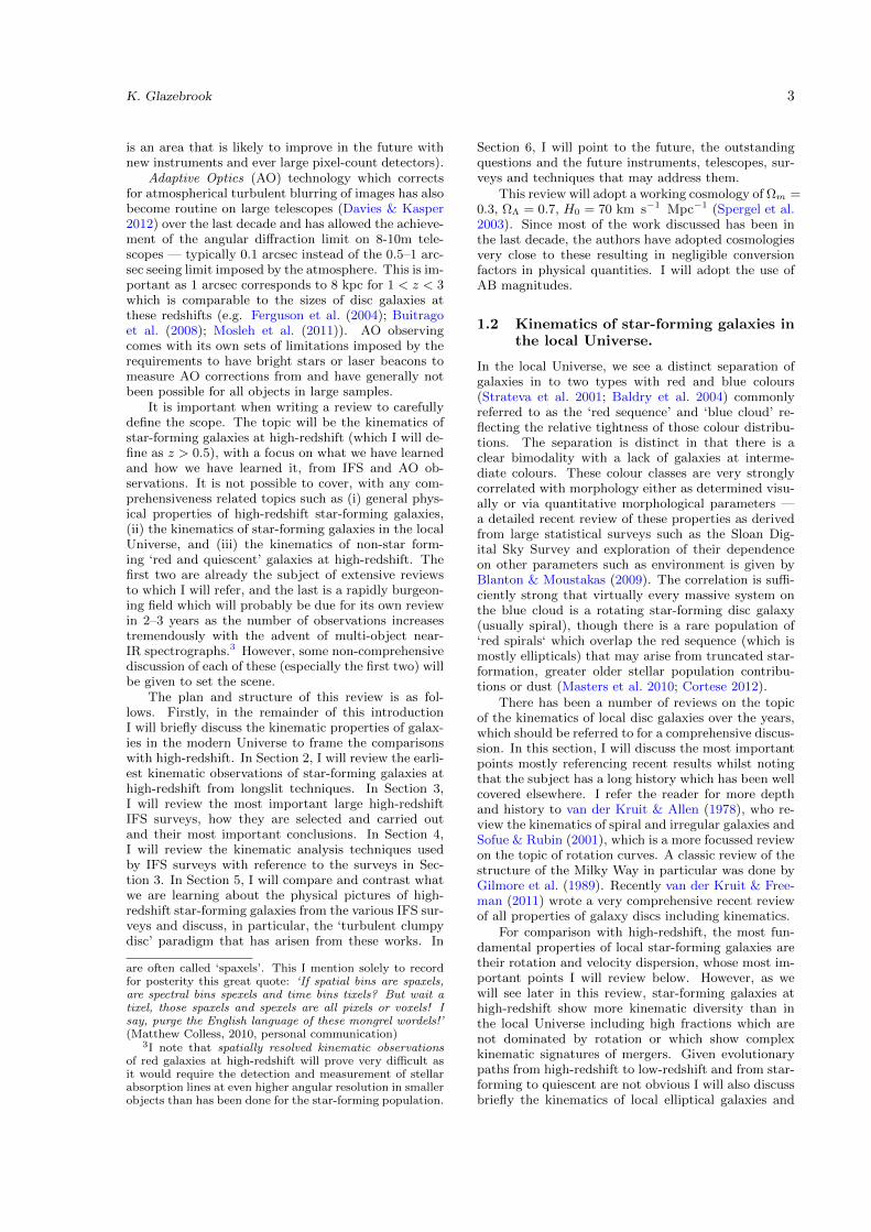
Figure 3: The distribution of the principal IFS surveys in the redshift (left) and star-formation rate — stellarmass (right) space (stellar masses are corrected to the Salpeter (1955) IMF). The lines on the right plot are thelocations of the main galaxy ‘star-formation main sequence’ at different redshifts taken from the models of Boucheet al. (2010). Credit: adapted from Figures 10 & 14 of Contini et al. (2012), reproduced with permission c© ESO.

well as rest UV-selected galaxies (the latter sub-samplewas the focus of the early work of Forster Schreiberet al. (2006)). These formed the majority of the thesample and the various papers focussed on these, inparticular with the Hα detected sub-sample with 1.3 <z < 2.6 (62 galaxies). A large range of stellar masswas probed (2 × 109 – 3 × 1011M with a median of2.6×1010M) as the K-band and UV selection tendedto pick up complementary populations.

A primary result (echoed in other work) summarisedin the survey paper (Forster Schreiber et al. 2009)was that around a third of the sample were rotat-ing star-forming discs (Forster Schreiber et al. 2006)with large ionised gas dispersions (‘turbulent discs’)with vc/σ ∼ 2–4. Another third were objects withno significant kinematic shear but still high disper-sion (‘dispersion dominated galaxies’ in the languageof Law et al. (2007)) while the remaining third had de-tectable kinematic structure but no clear disc-like pat-tern, so they were described as ‘clear mergers’. Thisapproximately 1/3:1/3:1/3 split of fundamental kine-matic classes is echoed in many other surveys we willsee in this section though the exact percentages vary.Morphologically, the discs do not resemble local spi-rals of similar mass, rather they are dominated by gi-ant kpc scale clumps of emission — and this remainstrue whether UV, Hα or near-infrared continuum isconsidered (Forster Schreiber et al. 2011).

Cresci et al. (2009) presented the kinematics of thebest quality SINS discs (Figure 4), mostly those withthe highest signal:noise ratio and/or AO observations.These are generally massive star-forming galaxies withK < 22.4 and quite large (disc scale lengths of 4–6kpc). The dynamical modelling of the discs required alarge component of isotropic velocity dispersion (40–80km s−1), construction of the stellar mass Tully-Fisher

relationship indicated a 0.4 dex9 offset at z ∼ 2 lowerin stellar mass at a given vc and is plausibly repro-duced by simulated galaxies. Puech et al. (2008) raisethe question about the choice of local relation whichcan have an effect on the amount of evolution; Verganiet al. (2012) argue this makes negligible difference tothe results of Cresci et al. as the different local rela-tions intersect at 1011M which is the mass range ofthe SINS discs considered. Bouche et al. (2007) con-sider the other velocity–size scaling relation of SINSgalaxies (using half-light radii) and concluded this re-lation was evolved from z = 0.

Clearly distinguishing discs from mergers kinemat-ically is a key issue (to which I will return in the nextsection), Shapiro et al. (2008) considered this for asample of 11 SINS galaxies (again highest signal:noise)using the technique of ‘kinemetry’ (Krajnovic et al.2006), they find 8/11 are discs by this criterion andclassify the rest as mergers, though dispersion-dominatedobjects were excluded as the sample was biassed to-wards well-resolved objects.

The resolved physical properties of SINS discs wasaddressed in a series of papers, Genzel et al. (2008)considered possible scenarios for the origin of the tur-bulence and the evolution of the discs. They arguethat the large dispersions applies to cold gas as wellas the observed ionised gas and arises from cosmolog-ical accretion. There is a correlation of central massconcentration with metallicity (as inferred from the[NII]/Hα line ratio) which which would imply that bul-geless galaxies are younger. Newman et al. (2013) con-sidered an extended AO sample and compared withnon-AO observations, in particular finding that thefraction of ‘dispersion dominated’ galaxies (see Sec-

9All dex values reported in this review refer are in logmass or log luminosity unless otherwise stated.


Figure 4: Three selected z ∼ 2 galaxies from Cresciet al. (2009) well fit by kinematic disc models. Themiddle object, galaxy D3a-15504, was originally ob-served by Genzel et al. (2006), here it has higher sig-nal:noise. These are Hα emission line maps, top twotaken with AO at resolution 0.2 arcsec, the bottom ob-ject illustrates how these disc kinematics are still re-solved in natural seeing. On the left are the kinematicmaps (top row: velocity, bottom row: dispersion) com-paring the data and best fit disc models. Hα intensitymaps are shown on the top right. Each galaxy is well fitby a rotating disc model but the velocity dispersion ishigh. Values reach > 100 km s−1. I call out the spatialstructure in the dispersion maps (see my discussion inSections 5 and 6.1) as a particular striking and unex-plained feature, not reproduced in the models. Credit:adapted from Figure 2 of Cresci et al. (2009) (selectedgalaxies), reproduced by permission of the AAS.

tion 5.2) drops with increasing resolution. Genzel et al.(2011) considers the properties of the giant kpc clumpsof five galaxies in more detail. Key points are that theclumps are entrained in the overall rotation field of thedisc (i.e. they are part of the disc not merging externalgalaxies), that they occur in regions of disc instabilityas indicated by Toomre Q < 1 and that they showbroad wings10 indicative of star-formation-driven out-flows (Newman et al. 2012b).

10An important point is that these are even broader wings(several hundred km s−1 width) on a central componentwhich is often confusingly called ‘narrow’ despite beingbroader than in local disc galaxies.

3.2 The OSIRIS survey of UV-selected galax-ies

The IFS survey of Law et al. (2007, 2009) focussed on13 UV-selected galaxies observed with the OSIRIS IFS(Larkin et al. 2006) on the Keck telescope.11 Twelveof these galaxies are at z ∼ 2.2 selected using the‘BX’ colour criteria of Steidel et al. (2004) and were asubset with high Hα fluxes from previous slit spectra(Erb et al. 2006a) or high star-formation rates calcu-lated from rest-frame UV emission. The IFS subsetwas mostly selected on the emission line fluxes butalso had a subjective selection component for inter-esting objects with criteria such as extreme ends ofthe young/low mass old/high-mass scales, multicom-ponent UV morphology, and unusual UV spectra. Alower z ∼ 1.6 sample also selected from the BM/BXcatalogue and observed by the complementary projectof Wright et al. (2007, 2009); this is described belowalong with other OSIRIS work at similar redshifts (Sec-tion 3.6).

The Law et al. sample galaxies are generally oflower stellar mass (1× 109–8× 1010M with a medianof 1.4× 1010M) by a factor of 2 than the SINS discsat the same redshift; however, there is a broad over-lap (Figure 3). All IFS observations where done withlaser guide stars (LGS) AO of the Hα line in the K-band so that spatial resolution was 1–2 kpc, severaltimes better than non-AO observations of other sur-veys. The price to be paid for this was the lower sur-face brightness sensitivity for extended emission dueto the finer pixel sampling and the reduced flux fromfinite Strehl (' 0.3). From the IFS observations, 6/13galaxies showed clear velocity shears, though mergerinterpretations were also plausible in 3–4 of these, with1–2 being very clear discs.

Law et al. note the dominance of objects withhigh intrinsic dispersions 50–100 km s−1 which werein all cases larger than the maximum velocity shearamplitude (another contrast to the SINS discs), la-belling these ‘dispersion dominated galaxies’. Someobjects had no detectable shear whatsoever. In thecomparison of Forster Schreiber et al. (2009), it wasshown that the typical ‘circular velocities’ (under adisc interpretation) and half-light radii (measured inHα) were also a factor of 2–3 smaller than SINS discs,with the smallest Law et al. objects having sizes of. 1 kpc. This seems consistent with a broader picturewhere UV-selection favours lower stellar mass, smallerstar-forming galaxies at these redshifts and is furtherdiscussed in Section 5.2.

Law et al. (2007) looked at the ‘Toomre parameterQ’ in three objects as defined by:

Q =V 2

GMdisc/rdisc= Mdyn/Mdisc (1)

where V is the observed shear. However, this equa-tion does not correspond well to the standard Toomre(1964) criterion — though one can obtain it by writingσ = V . It is better thought of as a ratio of dynam-ical mass (rV 2/G) to visible ‘disc’ mass (Mdisc), the

11The lack of an acronym is, in my opinion, refreshing.

K. Glazebrook 11

galaxies all had Q . 1 indicating that the disc massis unphysical — i.e. too much mass to be supporteddynamically by rotation. I also note that interestinglythe equation corresponds very closely to the criterionfor exponential disc instability (against bar formation)in a dark matter halo independently identified by Moet al. (1998) (their eqn. 35). The ‘Q’ values suggestthey may be true dispersion-dominated objects andnot stable discs, unless the compactness causes V tobe significantly underestimated through resolution ef-fects (and their could also be issues with inclinationwhich is not accounted for).

It is important to note that Law et al. observeda similar number of galaxies which were not detected,there was a tendency for these objects to be observed insub-optimal conditions (e.g. seeing) but there could bea result of a bias of detections to higher surface bright-ness. The authors do find a systematic trend in thedirection expected for this bias compared to the gen-eral galaxy population at this redshift. Interestingly,one of the non-detections was subsequently detectedby Law et al. (2012a) with a five times longer OSIRISexposure, it proved to be a high-dispersion rotatingdisc with a spiral pattern (rare at these redshifts, at-tributed to a minor merger induction). Three morewere observed and also detected by Forster Schreiberet al. (2009) in natural seeing and proved to be rotationdominated, clearly the resolution–sensitivity trade ofAO observations is playing a role (as did the longerexposures used).

The incidences of possible discs and mergers seemcomparable with other work (perhaps with a trend toless of these at lower stellar masses), however the com-pactness of these galaxies does not lead to unambigu-ous characterisation and Law et al. caution againstover-simplistic classifications in to these two classes.

3.3 The IMAGES and related FLAMES-GIRAFFE surveys

The predominant IFS work at intermediate redshift(0.3 < z < 1) has been done using the VLT’s FLAMES-GIRAFFE multi-object integral field facility. This hasproduced a large sample from the IMAGES (‘ Interme-diate MAss Galaxy Evolution Sequence’) VLT LargeProgram. FLAMES-GIRAFFE (Pasquini et al. 2002)is an optical facility with 15 separate ‘Integral FieldUnits’ (IFUs) patrolling a 25 arcmin field-of-view.

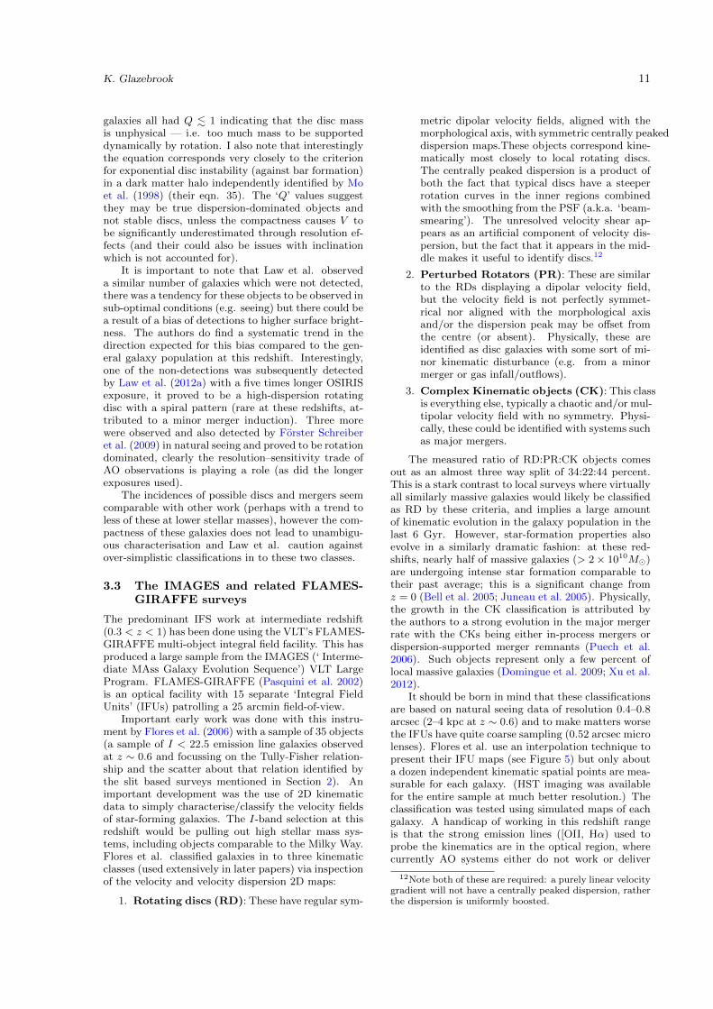
Important early work was done with this instru-ment by Flores et al. (2006) with a sample of 35 objects(a sample of I < 22.5 emission line galaxies observedat z ∼ 0.6 and focussing on the Tully-Fisher relation-ship and the scatter about that relation identified bythe slit based surveys mentioned in Section 2). Animportant development was the use of 2D kinematicdata to simply characterise/classify the velocity fieldsof star-forming galaxies. The I-band selection at thisredshift would be pulling out high stellar mass sys-tems, including objects comparable to the Milky Way.Flores et al. classified galaxies in to three kinematicclasses (used extensively in later papers) via inspectionof the velocity and velocity dispersion 2D maps:

1. Rotating discs (RD): These have regular sym-

metric dipolar velocity fields, aligned with themorphological axis, with symmetric centrally peakeddispersion maps.These objects correspond kine-matically most closely to local rotating discs.The centrally peaked dispersion is a product ofboth the fact that typical discs have a steeperrotation curves in the inner regions combinedwith the smoothing from the PSF (a.k.a. ‘beam-smearing’). The unresolved velocity shear ap-pears as an artificial component of velocity dis-persion, but the fact that it appears in the mid-dle makes it useful to identify discs.12

2. Perturbed Rotators (PR): These are similarto the RDs displaying a dipolar velocity field,but the velocity field is not perfectly symmet-rical nor aligned with the morphological axisand/or the dispersion peak may be offset fromthe centre (or absent). Physically, these areidentified as disc galaxies with some sort of mi-nor kinematic disturbance (e.g. from a minormerger or gas infall/outflows).

3. Complex Kinematic objects (CK): This classis everything else, typically a chaotic and/or mul-tipolar velocity field with no symmetry. Physi-cally, these could be identified with systems suchas major mergers.

The measured ratio of RD:PR:CK objects comesout as an almost three way split of 34:22:44 percent.This is a stark contrast to local surveys where virtuallyall similarly massive galaxies would likely be classifiedas RD by these criteria, and implies a large amountof kinematic evolution in the galaxy population in thelast 6 Gyr. However, star-formation properties alsoevolve in a similarly dramatic fashion: at these red-shifts, nearly half of massive galaxies (> 2× 1010M)are undergoing intense star formation comparable totheir past average; this is a significant change fromz = 0 (Bell et al. 2005; Juneau et al. 2005). Physically,the growth in the CK classification is attributed bythe authors to a strong evolution in the major mergerrate with the CKs being either in-process mergers ordispersion-supported merger remnants (Puech et al.2006). Such objects represent only a few percent oflocal massive galaxies (Domingue et al. 2009; Xu et al.2012).

It should be born in mind that these classificationsare based on natural seeing data of resolution 0.4–0.8arcsec (2–4 kpc at z ∼ 0.6) and to make matters worsethe IFUs have quite coarse sampling (0.52 arcsec microlenses). Flores et al. use an interpolation technique topresent their IFU maps (see Figure 5) but only abouta dozen independent kinematic spatial points are mea-surable for each galaxy. (HST imaging was availablefor the entire sample at much better resolution.) Theclassification was tested using simulated maps of eachgalaxy. A handicap of working in this redshift rangeis that the strong emission lines ([OII, Hα) used toprobe the kinematics are in the optical region, wherecurrently AO systems either do not work or deliver

12Note both of these are required: a purely linear velocitygradient will not have a centrally peaked dispersion, ratherthe dispersion is uniformly boosted.


Figure 5: Images and IFS maps of galaxies of different kinematic classes from sample FLAMES/GIRAFFE datashowing the different kinematic classifications described in the text. Note the rather coarse spaxel scale of 0.52arcsec (see grid superimposed on higher-resolution HST image) makes classification challenging and a 5× 5 pixelinterpolation scheme was used to smooth the maps. Credit: adapted from Figures 3 & 5 (selected galaxies andcombined) of Flores et al. (2006), reproduced with permission c© ESO.

negligible Strehl. So it is not even possible to ob-serve sub-samples with AO (as for example SINS didat z ∼ 2). As AO systems improve and work at bluerwavelengths this may be remedied in the future.

Flores et al. construct a Tully-Fisher relationshipand their most important conclusion was that the largeresidual scatter identified in slit surveys arose from thenew kinematic PR, CK classes. The Tully-Fisher re-lationship for the RD class alone shows reduced scat-ter comparable to the local relation. The RD relationalso shows no detectable zero point offset from the lo-cal stellar mass Tully-Fisher relationship of Verheijen(2001), this is in contrast to previous slit-based work.The authors attribute this to the strong evolution inkinematic classes and the inability of slit surveys todistinguish these classes as the kinematics is only mea-sured along a single slice through the galaxy. The RDclass does appear to have a significantly higher velocitydispersion and consequent lower v/σ than local galax-ies (Puech et al. 2007) echoing the trend found in z ∼ 2galaxies. The PR class extends this trend to even lowerv/σ values.

The IMAGES large program (Yang et al. 2008) wasan extension of this earlier FLAMES-GIRAFFE workto double the sample size to 63 galaxies over a similarredshift range. From an I-band selected input red-shift survey of galaxies with [OII] emission, they aredown-selected by rest-frame J-band luminosity, cor-responding to an approximate stellar mass limit of> 1.5 × 1010M at the redshift of the survey. Yanget al. confirmed the evolution of the kinematic classfractions, with similar values to those quoted above.Neichel et al. (2008) examined the relation betweenmorphological and kinematic classes and found a verystrong correlation between the RD objects and galax-

ies that appeared in HST images as spiral discs. TheTully-Fisher relationship was explored in more detailby Puech et al. (2008) who reaffirmed the earlier con-clusion that the increase in scatter about the mean re-lation was due to the ‘non-relaxed’ PR and CK classes(the scatter increases from 0.1 to 0.8 dex from RDsto CKs; shown in Figure 6). However, with a biggersample and an improved analysis and a revised localreference13, they now found a modest amount of zeropoint evolution in the K-band Tully-Fisher relation-ship (about 0.34 dex or a factor of two in stellar mass atfixed velocity since z ∼ 0.6). The high star-formationrate of z ∼ 0.6 galaxies implies they are likely to bemuch more gas rich than local spirals. Puech et al.(2010) tried to incorporate this gas in to the massbudget by inverting the Kennicutt-Schmidt relation-ship (Kennicutt 1989) between gas and star-formationsurface density14 and construct a baryonic Tully-Fisherrelationship. They find that the zero point of this re-lation does not evolve, that galaxies in their samplehave approximately equal stellar and gas masses, andhence conclude that the evolution of the stellar massTully-Fisher relationship simply reflects the conversionof this gas in to stars since z ∼ 0.6.

13The local stellar mass relation was based on the K-band one of Hammer et al. (2007), which they derive fromthe SDSS relation of Pizagno et al. (2007). Hammer et al.examine the Verheijen relation (which is also the basis ofthe Bell & de Jong (2001) relation) and conclude that it isbiased and the SDSS relation is more reliable.

14A recent review of such ’Star-Formation Laws’ innearby galaxies is presented by Kennicutt & Evans (2012).

K. Glazebrook 13

Figure 6: Stellar mass Tully-Fisher relationship at z ∼0.6 from the IMAGES survey showing the dependenceof the increase of scatter as the kinematic class goesfrom regular discs to objects with irregular kinematics.Credit: adapted from Figure 3 (left panel) of Puechet al. (2010), reproduced with permission c© ESO.

3.4 The MASSIV survey

The Mass Assembly Survey with SINFONI (MASSIV)sample is an IFS survey at 0.9 < z < 1.8 of 84 galax-ies, 11 with AO-LGS (Contini et al. 2012). Selection isfrom the VVDS redshift survey (Le Fevre et al. 2005)either using the [OII] emission line strength or rest-frame UV luminosity at the higher redshift end, andwith a hierarchical selection scheme (‘wide’, ‘deep’ and‘ultra-deep’ VVS parent samples). Early results frompreliminary samples were presented on kinematic clas-sification (Epinat et al. 2009). The full survey descrip-tion of Contini et al. shows a comparison in the star-formation rate-stellar mass main sequence plane withother samples (reproduced in Figure 3). The distribu-tion of star-forming galaxies at 1 < z < 2 is reasonablysampled by MASSIV, though of course their might bebiases (e.g. against dusty star-formers without UV orline emission) and there is a deficit of the very massive(> 1011 M) star-forming galaxies sampled by SINS atz > 2.

Epinat et al. (2012) presents an analysis of thekinematical distribution. After considering multiplepossible classification parameters (strength of veloc-ity shear, kinematic/morphological alignment, residu-als to disc fits, velocity dispersion maps, presence ofcompanions — B. Epinat, 2013, private communica-tion), the team settled on two principal classificationdimensions. The first was between ‘rotators’ (44%)and ‘non-rotators’ (35%) with the remaining 21% nothaving sufficient signal:noise to classify. The secondwas between isolated and merging / interacting galax-ies, the latter make up 29% of the entire sample butit is important to note that there is some overlap (e.g.some rotators are interacting). This categorisation is

rather different to the classifications done in the othersurveys (e.g. SNS, IMAGES) where for example rota-tors and mergers are exclusive categories. This partlyarises from the fact that the identification of merg-ers in MASSIV comes from the presence of multiplecomponents (separated spatially and kinematically) intheir IFS images, this is different from the approach ofidentifying irregular velocity maps. That said, thereis a considerable overlap between the non-rotators andmergers (about half of non-rotators are classified asinteracting vs only 20% of rotators) and the isolatednon-rotators tend to be smaller. Thus, if one were tothink of this in terms of the disc:merger:dispersion-dominated trichotomy of other surveys, the fractionsare similar — a roughly three way split. Lopez-Sanjuanet al. (2013) present a more detailed analysis of themerger rate in the sample, taking advantage of thewide-field of the SINFONI IFS (∼ 70 kpc at z ∼ 1.3)to systematically define the close pair fraction by spa-tial proximity and separation in redshift. This is aunique IFS science application; imaging surveys cannot determine the association along the line of sightand long-slit observations do not cover enough sky areato find non pre-selected secondary objects. Of coursethe IFS approach does require the companion to haveemission lines above a detection limit, as such theyare only sensitive to gas-rich mergers. They found amerger fraction of ' 20% across a range of redshift;using a time-scale model this was translated in to amerger rate and cumulative merger number for mas-sive galaxies over 0 < z < 1.5. I discuss the mergerrate and the comparison with other techniques in moredepth in Section 5.4.

The ‘rotator’ classification is made by consideringfractional residuals from a fitted disc model vs align-ment between kinematic and morphological axis (I dis-cuss this further in Section 4.5). Rotating galaxies arefound to be larger and have higher stellar masses andstar-formation rates (typically by a factor of two ineach), a result similar to other surveys. The typicaldisc velocity dispersion is found to be ∼ 60 km s−1.Comparing with the SINS/AMAZE/LSD samples athigher redshift, and the lower redshift IMAGES andthe local GHASP (Epinat et al. 2010) samples, ev-idence is found for a smooth evolution in disc localvelocity dispersions. Interestingly, similar dispersionsare found for rotators and non-rotators, with the lat-ter having a strong anti-correlation between size anddispersion.

Vergani et al. (2012) presents the Tully-Fisher re-lationship and size-velocity scaling relations and againcompare with the IFS samples at different redshifts.The rotators at < z >' 1.2 show consistency witha small scatter stellar mass Tully-Fisher relationship,whilst the non-rotators depart radically from this. Thequestion of evolution depends on which local Tully-Fisher relationship is assumed (an issue also highlightedby Puech et al. (2008)), but the comparison with Piza-gno et al. (2007) suggests a −0.36 dex evolution of thezeropoint fairly similar to that found by SINS (Cresciet al. 2009) at z ∼ 2, consistent with the idea of discsincreasing their stellar mass with time at a fixed vc.Consistent gas fractions were found using both the


Kennicutt-Schmidt relationship and the difference be-tween dynamical and stellar mass. The baryonic Tully-Fisher relationship does not appear evolved since z = 0similar to the findings of Puech et al. Size-velocity evo-lution in MASSIV appears modest (at most 0.1 dexsmaller sizes at high-redshift at a given stellar mass).

3.5 The AMAZE/LSD surveys

The AMAZE (‘Assessing the Mass-Abundances Z Evo-lution’) and LSD (‘Lyman-Break Galaxies Stellar Pop-ulations and Dynamics’) are two related surveys (bysubstantially the same team, and usually analysed jointly)using SINFONI of galaxies at z > 3, a substantiallyhigher redshift than the other large surveys. AMAZEMaiolino et al. (2008) targeted UV-selected galaxies(classical LBG selection) mostly at 3 < z < 3.7 (U -band dropouts) with a few at 4.3 < z < 5.2 (B-band dropouts) from deep spectroscopic surveys in theChandra Deep Field South and performed observationsin natural seeing (0.6–0.7 arcsec PSF). LSD (Mannucciet al. 2009) employed a similar LBG selection at z ' 3and focused on natural guide star AO observations,drawing on the large catalog of Steidel et al. (2004) tofind objects near suitable AO stars. Typical magni-tudes were R . 24.5 corresponding to a mass range of1010−11M at z ' 3. Some lensed galaxies were alsoincluded but their analysis has not been published.

Gnerucci et al. (2011b) presented the kinematicanalysis of the AMAZE/LSD samples, in particular 23AMAZE and 9 LSD galaxies all in the range 2.9 <z < 3.7 apart from one object at z = 2.6. Theypresented a two-stage approach to identifying rotatingdisc galaxies: first, they fitted a simple linear velocityshear model to the IFS maps. Galaxies with statis-tically significant shear were classed as ‘rotating’ andthen subject to full disc model fitting. An advantageof this approach is that fitting a shear requires sub-stantially less model parameters and is more robustin low signal:nose data. This gave some quite inter-esting results which shed light on the comparisons ofother surveys: 10/23 of the AMAZE galaxies but only1/9 of the LSD galaxies were rotators. In my view,this is quite a significant difference given the very sim-ilar and comparable selection and observations of theAO and non-AO samples and the previous compar-isons of the SINS (mostly non-AO, larger fraction ofrotation-dominated discs) and OSIRIS (all AO, mostlydispersion-dominated) samples. It is likely that atleast part of this is due to the greater sensitivity of thenon-AO observations to the low surface brightness ex-tended, rotating, outskirts of disc galaxies as Gnerucciet al. note. There was no overlap between AO andnon-AO samples.

For the rotators, estimates of dynamical mass wereconstructed from the modelling and were consistentwith large gas fractions (up to 90%) when comparedto the stellar mass. Gnerucci et al. compared thisto the gas masses inferred another way by invertingthe Kennicutt-Schmidt relationship and found a plau-sible 1:1 correlation. The v/σ ∼ 2 values of the rota-tors were a factor of two less than that of SINS discsat z ∼ 2, which seems consistent with the higher gas

fractions compared to z ∼ 2 in the framework of the‘turbulent gas-rich disc’ model (see Section 5.1). TheTully-Fisher relationship of the discs was consistentwith a large −1.0 dex decrease in the stellar mass ata given velocity relative to local galaxies, substantial-ity more than at z ∼ 2, but with a very large scatter(∼ 0.5 dex).

Other AMAZE/LSD papers considered the evo-lution of the stellar mass:global metallicity relation(Mannucci et al. 2010, 2009) and the discovery of pos-itive metallicity gradients (i.e. metal poor galaxy cen-tres) in a sub-set of galaxies (Cresci et al. 2010).

3.6 Other optical/near-infrared IFS surveysat z > 1

As well as the large surveys, several smaller projectsshould be mentioned, these tend to probe complemen-tary parameters spaces.

In particular in the 1 < z < 2 regime AO is possi-ble, but difficult, since one must target Hα in the near-infrared H-band where it has reduced Strehl. Wrightet al. (2007, 2009) present OSIRIS AO kinematics ofseven galaxies at 1.5 < z < 1.7 UV-selected and withprior optical spectroscopy using the BM/BX criterion.They find four of these to have kinematics consistentwith disc systems and high intrinsic velocity disper-sions (> 70 km s−1) in at least two of these. Wis-nioski et al. (2011) presents OSIRIS AO kinematicsof 13 galaxies a ∼ 1.3, again selected by rest-frameUV emission and optical spectroscopy, but selectedfrom a wider area survey probing higher UV luminosi-ties and star-formation rates higher than more typicalz ∼ 1.3 galaxies (but comparable to z > 2 SINS disc).They again find that around half the objects have disc-like kinematics and high intrinsic velocity dispersionsand clumpiness. The resolved star-formation proper-ties and clump scaling relations were examined furtherin Wisnioski et al. (2012). An interesting difference be-tween the Wright et al. and Wisnioski et. al. sampleslies in the nature of the non-disc candidates — in thefirst they are extended objects with multiple sources ofresolved Hα emission and irregular kinematics whereasin the latter they tend to be single compact sources ofHα emission with mostly dispersion-dominated kine-matics (i.e. similar to the Law et al. objects at z > 2illustrated in Figure 13). It is not clear if this reflectsthe different selection, luminosity and/or space den-sity, or simply the signal:noise of the data. More lu-minous Hα objects are easier to map; however, the ac-tual effect seems reversed in that the fainter non-discsources of Wright et al. tends to have more extendedHα morphologies.

An alternative selection technique to the broad-band-selected surveys mentioned above is via the use ofnarrow-band imaging which has the advantage that thegalaxies are already known to have the strong emissionlines required for successful IFS observations. Swin-bank et al. (2012b) observed with SINFONI 14 Hαselected emitters at redshifts 0.8, 1.5 and 2.2 corre-sponding to the wavelengths of their narrow-band fil-ters of the parent imaging sample (’HiZELS’, Sobralet al. (2009, 2013)), and with a stellar mass range sim-

K. Glazebrook 15

ilar to the SINS survey. AO IFS maps were obtainedfor nine of these galaxies, five of which were classifiedas discs (+ two mergers and two compact galaxies),again very similar fractions to other surveys. The stel-lar mass Tully-Fisher relationship was examined show-ing a factor of two evolution in mass at a fixed velocitysince z . 2. The discs themselves were physically verysimilar to SINS discs in that they had high dispersion,low v/σ values as well as clumpy star-formation andhigh gas fractions (Swinbank et al. 2012a). One par-ticularly interesting point was that two of the objectswith AO observations were at z = 0.84, though thereported Strehl was low (' 10%) as is normal withcurrent systems for J-band observations. Notably thisis the only AO IFS observations I know of for galaxiesat 0.3 < z < 1.

An especially powerful combination has been tocombine AO IFS observations with the gravitationalstrong lensing effect of giant clusters at intermediateredshift which can often magnify background galax-ies by factors of up to 10–50 (see the review of Treu(2010)). Such strong lensing only occurs over lim-ited sky areas, and the objects most magnified tendto be the faint but numerous objects not probed byother surveys. A key question is: do the sensitivityand coarser resolution limits of the non-lensed surveysgive us a biased view of the high-redshift population?The lensed surveys also allow us to probe z > 3 andsmaller spatial scales. Stark et al. (2008) (Figure 7)and Jones et al. (2010) consider a sample of six lensedsources magnified up to 50× at 1 < z < 3. They finda much higher-incidence of rotating, high-dispersiondiscs (4/6) than in the more luminous sources probedby unlensed surveys and in all cases the galaxies are re-solved in to multiple emission line clumps. Yuan et al.(2011, 2012) present observations of two more objectswhich again seem consistent with the picture of highdispersion, low v/σ clumpy discs. The highest redshiftexamples to date are two lensed z ∼ 5 galaxies (Swin-bank et al. 2007; Swinbank et al. 2009) observed in[OII] and with very low dynamical masses (109−10M)and velocity shears (< 100 km s−1) compared to theother surveys but still relatively large velocity disper-sions (∼ 80 km s−1). A particular benefit of the grav-itational lens observations is the use of the high linearmagnification to probe the size of star-forming clumps.Currently, only lensing can deliver ∼100 pc spatial res-olution of high-redshift galaxies, resolution is criticalfor accurate size measurements and hence testing thepicture of large high-Jeans mass clumps in unstablediscs (Jones et al. 2010; Livermore et al. 2012). Iwill return to this scenario in Section 5.1. Two morenotable lensed objects are presented in (a) Nesvadbaet al. (2006) of a giant arc at z ∼ 3 whose de-lensedkinematics suggests a rotating disc and (b) Nesvadbaet al. (2007) a lensed sub-mm galaxy with merger-likekinematics.

In addition to the MASSIV survey, other samplesof galaxies selected from the VVDS sample have beenobserved with SINFONI (non-AO). Lemoine-Busserolle& Lamareille (2010) present a sample of ten 1.0 < z <1.5 galaxies selected on their [OII] emission, findingeight rotating high-dispersion discs, one clear merger,

Figure 7: A beautiful example of a small disc galaxyat z = 3.07 with dynamical mass ∼ 2 × 109Mand star-formation rate ∼40 M yr−1 from Starket al. (2008) lensed 28-fold and demonstrating a near-complete Einstein Ring observed at ∼100 pc resolutionwith the assistance of gravitational lensing and AO.Maps on the left show (a) lens reconstructed rest-UVcontinuum (∼1500A) emission, (b) [OIII] 5007]A lineemission (with contours showing Hβ), (c) velocity mapand rotation curve showing a characteristic ‘spider di-agram’ and (d) dispersion map and curve (tilted linesshow extraction axis). (See Stark et al. for full fig-ure details.) The galaxy is clumpy in continuum andline emission but is a clear disc with a turnover andhigh dispersion in the kinematics. The top-right panelshows the original sky plane image (composite red: K-band, green: [OIII], blue: HST V606 filter) known asthe ‘Cosmic Eye’ with the red central source being thez ∼ 0.7 lens. Credit: adapted from Figures 1 & 2 ofStark et al. (selected panels and combined), reprintedby permission from Macmillan Publishers Ltd: Nature,455, 775 c© 2008.

and one object with no kinematic variation interpretedas face-on. They split the discs almost equally be-tween ‘rotation dominated’ and ‘dispersion dominated’around v/σ = 1.66 which appear to follow relativelyoffset stellar mass Tully-Fisher relationship relations(and both evolved from the local relation). Lemoine-Busserolle et al. (2010) select three intermediate stellarmass (1–3×1010 M) z ∼ 3 galaxies from VVDS basedon their rest-frame UV VVDS spectra and observed inthe near-IR in Hβ, [OIII] lines. They have very highstar-formation rates for this redshift — as a result ofbeing selected as I < 24 in VVDS they are brighter

http://www.nature.com


in the rest frame UV than typical z ∼ 3 galaxies. Allthree have high dispersion and small shears (v/σ . 1),one was tentatively classified as a merger based onanomalous kinematics, and the other two were con-sistent with rotating disc models. However, interest-ingly, both of the latter displayed secondary compo-nents consistent with close companions. The typicalvelocity shears are small (< 50 km s−1) and they ar-gue the properties of the sample are very similar tothose of the Law et al. objects at z ∼ 2. Anotherz ∼ 3 LBG observed with SINFONI is presented byNesvadba et al. (2008), this is interpreted as a merger.

3.7 Sub-mm line surveys

All of the surveys presented so far, and a majority ofthe discussion, has focussed on 2D kinematics mea-sured using rest-frame optical emission lines observedin the near-infrared. A change from this and an inter-esting development has been the first kinematic mea-surements at high-redshift using sub-mm wavelengthlines, so far of the CO molecule.

High-redshift star-forming galaxies are rich in molec-ular gas and dust. In particular, among the mas-sive star-forming galaxies, we see a population of ‘sub-mm galaxies’ (Blain et al. 2002) with strong emis-sions at these frequencies due to star-formation ratesup to 1000 M/yr per year (e.g. Micha lowski et al.(2010)). A strong correlation of star-formation ap-proximately proportional to stellar mass is observed athigh-redshift (the ‘star-forming main sequence’ (Noeskeet al. 2007; Daddi et al. 2007) but the classical ‘sub-mmgalaxies’ may lie above this relation and may representrare events such as major mergers (Daddi et al. 2010a).Main sequence massive star-forming galaxies at z ∼ 2have up to 50% gas fractions (Tacconi et al. 2010, 2013)several times higher than local massive spirals.

There are now over 200 total molecular gas mea-surements at high-redshift (e.g. see review of Car-illi & Walter (2013)), although the spatial resolutionis usually rather coarse (0.5–1.0 arcsec) due to thebaseline limitations of current sub-mm interferome-ters; however, this does allow some kinematic measuresfor larger galaxies. Early work by Genzel et al. (2003)using the IRAM Plateau de Bure Interferometer mod-eled the CO kinematics of a sub-mm-selected galaxyas a large rotating disc. Daddi et al. (2008) observeda more normal main-sequence galaxy and showed thatit was disc-like. The ‘PHIBSS’ CO survey of 52 mainsequence star-forming galaxies (Tacconi et al. 2010,2013) at z ∼ 1.2 and 2.2 found that 60% where kine-matic discs and that the CO velocity dispersions werehigh and agreed with the Hα values. This is an im-portant point as molecular gas is likely to dominatethe mass budget with ionised gas being only a smallfraction. A detailed spatial comparison of Hα opti-cal, NIR and CO data was performed for one of thesegalaxies by Genzel et al. (2013). They found that Hαand CO traced the same rotation curve and also evi-dence for variable dust extinction, an important caveatto be considered when interpreting optical maps.

There are only a handful of cases in the literaturewith kpc resolution and these are mostly objects with

a gravitational lensing boost to the resolution. Swin-bank et al. (2011) presented CO line observations ofthe z = 2.32 lensed sub-mm galaxy SMM J1235-0102which has a total star-formation rate of ∼ 400 M/yr(about 10× the ‘main sequence’ value for it’s mass).The beam was ∼ 0.5 arcsec and with the 30-fold lens-ing boost resolution of 100 pc was obtained. Despitethe extreme star-formation rate the CO kinematicsshowed that the molecular gas was distributed in aturbulent rotating disc (see Figure 8) with v/σ ∼ 4consistent with the picture inferred of other massivez ∼ 2 star-forming galaxies from ionised gas. Hodgeet al. (2012) analysed a single z = 4.05 very bright sub-mm galaxy where the CO lines are redshifted down tothe higher radio frequencies. Using a wide Very LargeArray spacing and 120 h of integration, they made amap at 0.2 arcsec resolution which revealed a clear discof dispersion ∼ 100 km s−1 with clumpy molecular gas(clump masses ∼ 109M). In contrast to these results,Hα kinematics of z ∼ 2 sub-mm galaxies have insteadfound that they mostly have complex velocity fieldswith multiple components showing distinct kinematicoffsets (Nesvadba et al. (2007); Alaghband-Zadeh et al.(2012) and notably Menendez-Delmestre et al. (2013)the first with AO). The origin of this difference be-tween kinematics in CO vs Hα is not clear but is likelydue to the small numbers of objects involved and het-erogenous selection. Of course the optical/near-IR se-lected general star-forming galaxy populations are alsodiverse but are somewhat better characterised.

With the ongoing deployment of ALMA (Hills &Beasley 2008), we can expect such observations to be-come routine, and expand to non-lensed samples ofnon-extreme objects, in the next few years.

3.8 Recent multislit surveys

While my main consideration in this review is IFSkinematic surveys in the last decade, it is necessaryto also mention some of the important kinematic re-sults from the more recent contemporaneous slit-basedsurveys as these have sampled much larger numbers ofhigh-redshift galaxies, albeit in 1D. These have mostlycome from the DEIMOS multi-object spectrograph onKeck (Faber et al. 2003) due to its relatively large slitmask area and high spectral resolution for kinematics.Weiner et al. (2006a,b) examined the Tully-Fisher re-lationship of ∼ 1000 galaxies at z . 1 in the ‘TeamKeck Redshift Survey’ using both integrated velocitydispersion (i.e. a similar idea to Forbes et al. (1996))and resolved rotation curve fits for the larger galaxies(∼ a third of the sample) and found strong evolutionin the B−band (fading with time) but little in thenear-infrared, with large scatter (0.3 dex) attributedto dispersion-dominated galaxies.

Kassin et al. (2007) looked at the stellar mass Tully-Fisher relationship of 544 galaxies (0.1 < z < 1.2)with resolved kinematic modelling from the DEEP2redshift survey (Newman et al. 2013a), as in earlierwork they found a large scatter (∼ 1.5 dex) at higherredshifts dominated by the more disturbed morpho-logical classes and the lower stellar masses and echo-ing the results from the IFS-based IMAGES survey

K. Glazebrook 17

Figure 8: Resolved CO velocity map of lensed z =2.32 sub-mm galaxy SMM J1235-0102 reconstructedin the source plane. This is one of only two pub-lished well-resolved molecular line velocity maps of ahigh-redshift disc galaxy. The effective lensing PSF(which is anisotropic) is shown as the white ellipse atthe top right. Contours are of velocity and the yellowcrosses are the locations of the star-forming clumps.The galaxy is well fit by a disc model, the inset showsthe residuals. Credit: from Figure 4 (top panel) ofSwinbank et al. (2011), reproduced by permission ofthe AAS.

at similar redshifts discussed earlier. Kassin et al.and Weiner et al. introduce a new kinematic measureS0.5 = 0.5 v2 + σ2, combining rotation and velocitydispersion and found the S0.5 Tully-Fisher relation-ship of all kinematic classes showed considerably re-duced scatter (∼ 0.5 dex) and no evolution in interceptnor slope (see Figure 15). The conclusion was that athigher redshifts, the star-forming galaxies are increas-ingly supported by dispersion arising from disorderedmotions (Weiner et al. 2006a). The M–S0.5 relationwas also found to agree with the local Faber-Jacksonrelation for elliptical galaxies suggesting a possible evo-lutionary connection. Also using DEEP2, FernandezLorenzo et al. (2009, 2010) considered the evolution ofthe Tully-Fisher relationship to z & 1 using integratedline widths to estimate rotation velocities of visuallyselected spirals; they found evolution in the B-bandconsistent with other studies but not in the K-band.However, when they consider the required evolution inK-band mass:light ratio with time, they conclude thatstellar mass may have doubled at fixed velocity in thelast 8 Gyr.

The recent DEIMOS survey of Miller et al. (2011)has provided a different, possibly conflicting, perspec-tive on Tully-Fisher relationship evolution. They ob-served only 129 0.2 < z < 1.3 galaxies but unlike pre-vious surveys, which were typically 1–2 h spectroscopicexposures, they took much longer 6–8 h exposures andtook care to align the slits to within 30 of the HST-

derived galaxy major axis. Like previous studies, theyfind evolution in the blue but little in the stellar massTully-Fisher relationship, but interestingly they reporta smaller scatter of only ∼ 0.06 dex in log10 v (0.2 dexin stellar mass), a factor of two less than in previoussurveys. This they attribute to their longer exposureswhich, for what they call ‘extended emission galax-ies’, means they can reach the flat-portion turnoverin 90% of their galaxies and place all of them on atight Tully-Fisher relationship and without requiringan extra parameter such as S0.5. This seems in contra-diction to the IFS results (primarily of the IMAGESsurvey) in the same redshift range. Nearly half the IM-AGES sample are the CK class which contribute ∼0.8dex of scatter and do not have regular disc-like kine-matics. It also seems to conflict with the kinematicfractions in the larger, but shallower, survey of Kassinet al. with the same spectrograph.

If the samples are broadly comparable, there is def-initely a contradiction. It is important to note thatMiller et al. only recover rotation velocities for 60% oftheir targeted sample (the remaining 40% are too com-pact in emission or have no emission) and that theydid not target 20% of their input sample as, again, be-ing too compact. It seems unlikely though that puresample effects can explain the discrepancy completely,as many of the Miller et al. galaxies have the pe-culiar/disturbed morphologies characteristic of othersamples. Perhaps the explanation is that deeper ob-servations of ‘CK objects’ show large-scale rotation?(And it can not simply be deeper observations reveal-ing shear from merging components as one would notthen expect them to lie on the Tully-Fisher relation-ship). The IMAGES survey also used 4–15 h expo-sures, though it is expected that an IFS instrumentmay have less throughput and the FLAMES-GIRAFFEsampling was relatively coarse. Interestingly, Miller etal. did observe three of the actual CK galaxies fromthe Flores et al. (2006) sample, noting the velocitieswere consistent within the IFS area. Comparing thetabulated properties of the objects in common, I notethat Miller et al. report masses 0.8–0.9 dex less forthese same three objects, with velocity agreement fortwo. These particular CK objects lie fairly close to theIMAGES Tully-Fisher relationship compared to otherCK objects, and all show distinct velocity shears inthe maps of Yang et al. (2008) and so may be mis-classified. They may not be comparable with the otherCK objects; a proper comparison would require moreoverlap.

Miller et al. (2012) extends their sample to 1.0 <z < 1.7 taking advantage of a newly installed extra-red sensitive CCD in the LRIS spectrograph on Keck(Rockosi et al. 2010). They successfully detected ex-tended emission and measure rotation curves in 42galaxies (out of 70 observed) and report a virtuallynon-evolving stellar Tully-Fisher relationship at theseredshifts (in conflict with Vergani et al. (2012)), againwith small scatter (Miller et al. (2013) attributes resid-ual scatter to bulgeless galaxies at z > 1 followingan offset —Tully-Fisher relationship). Again thereseems to be a conflict in kinematic classification, halfthe MASSIV sample at similar redshifts were classified


as non-rotating based on 2D IFS data (albeit severaltimes shorter exposure times). One must consider thatin these slit surveys, the slit angle must a priori be cho-sen from imaging data, it seems unlikely that one couldchoose this correctly to align with the rotation axis aswould be required to make a tight Tully-Fisher rela-tionship relation, given that MASSIV (Epinat et al.2012) reports that at least half of their sample arehighly misaligned. Is it possible that kinematic andphotometric alignment could only be revealed at lowsurface brightness on large scales? Is it really possi-ble to determine kinematic axes photometrically fromthe clumpy morphologies of galaxies at these redshifts?The implications of the disagreements apparent in theliterature are not yet clear.

These questions aside, there does seem to be gen-eral agreement between IFS and slit surveys on theincreasing contribution of internal velocity dispersionto disc kinematics. Kassin et al. (2012) (based on thesame DEEP2 sample) report a continuous increase indispersion to z = 1, matching with the IFS samplesat the same, or higher, redshift and consequent de-crease in v/σ. Interestingly, by defining a ‘disc set-tling criteria’ of v/σ > 3 (a value which they claimcorrelates with normal vs disturbed physical and kine-matic morphologies), they find a ‘kinematic downsiz-ing’ trend with stellar mass in the sense that high-massgalaxies ‘settle’ at earlier times (for example 50% of10.3 < log(M/M) < 10.7 galaxies are settled at z = 1compared with 90% at z = 0.2).

3.9 ‘Local analogue’ samples

A couple of groups have published IFS kinematics ofrare samples of nearby galaxies that are possible ana-logues of high-redshift populations.

The ‘Lyman-Break Analogues’ (LBAs) are galaxiesat z ∼ 0.2 selected as Lyman dropouts from space-UVobservations from the GALEX satellite. In particu-lar, Heckman et al. (2005) define a population withvery similar UV luminosity, stellar masses, and star-formation rates to z ∼ 3 LBGs and divide them into ‘compact’ and ‘large’ categories based on UV sizeand surface brightness. The large LBAs have stellarmasses of ∼ 1011 M, lower surface brightnesses andsizes of up to 10 kpc, the compact LBAs are typicallya factor of ten less massive and sizes < 2 kpc. Theydisplay similar colours and metallicities to the LBGs(Overzier et al. 2010) and similar morphologies domi-nated by large clumps of star-formation (Overzier et al.2008, 2009).

At these modest redshifts, it is possible to do AOobservations using the Paschen-α line in the K-band,which is not possible at zero redshift as it falls in theabsorption trough between the H and K-bands. ForCase B recombination (Hummer & Storey 1987) Pa-αis 12% the intensity of Hα (in the absence of dust —any extinction would make the ratio more favourable)however it is easily detectable in such nearby galaxieswith excellent spatial resolution. A high-luminositysubset of the compact population (dubbed ‘supercom-pact’) has been followed up by AO IFS using OSIRIS(Basu-Zych et al. 2009; Goncalves et al. 2010) and re-

veal themselves to be excellent analogues to the dis-persion dominated galaxies studied by Law et al. atz ∼ 2. They have high ionised gas dispersions (50–130km s−1), some evidence of small rotation/kinematicshears and low v/σ . 1 all very similar to the prop-erties of the Law et al. sample. This was confirmedby carrying out an ‘artificial redshifting’ computationto simulate the appearance of the galaxies to OSIRISand SINFONI at z ∼ 2. Overzier et al. (2008) andGoncalves et al. (2010) concluded that LBAs are mainlymergers based on HST morphology and OSIRIS kineme-try.

More recently, Green et al. (2010) and Green et al.(2013) analysed an IFS sample of nearby (z ∼ 0.1) butrare galaxies selected on their high Hα luminosity fromSDSS spectra. In galaxies with L(Hα) > 1042 erg/sthey made kinematic maps at ∼ 2 kpc resolution inHα (natural seeing observations) and identified galax-ies with high ionised gas dispersion(> 50 km/s), abouttwo-thirds of which were discs. This high-incidence ofrotation, the large stellar masses (up to 1011M andlarge sizes (2–10 kpc) suggest that they could be moresimilar to z ∼ 2 discs than LBAs; however, furtherwork and higher spatial resolution observations (seediscussion in Davies et al. (2011)) are required to con-firm this.

Another interesting set of local analogues are ‘tad-pole’ galaxies which have a ‘single clump + tail’ mor-phology. These were first identified at high-redshift byvan den Bergh et al. (1996) where their incidence ishigher. A handful have since been identified locallyin the SDSS survey (Straughn et al. 2006; Elmegreen& Elmegreen 2010). Elmegreen et al. (2012) foundthese to constitute 0.2% of UV bright surveys (com-pared to 6% of high-z galaxies; Straughn et al. (2006))and have stellar masses . 109 M; they attribute themorphology to lop-sided star-formation. The clumpshave masses of 105−7M; the galaxies appear to resem-ble scaled-down high-redshift tadpoles. The tadpoleshave high Hα velocity dispersion and show evidence formarginal rotation dominance (Sanchez Almeida et al.2013). Yet another class of rare low mass galaxieswhich might be similar to high-redshift objects are the‘green peas’ 15 first discovered by public volunteers in-specting SDSS images in the Galaxy Zoo project (Car-damone et al. 2009). These are very compact (2–3 kpc)low mass (108–1010M) but with high star-formationrates (> 10–30 M yr−1), low metallicities and havecomplex kinematics with velocity dispersions of 30–80 km s−1 (Amorın et al. 2012) suggesting similarities(apart from the substantially lower stellar masses) tothe ‘dispersion-dominated’ objects seen at high-redshift(see Section 5.2). Only a limited amount of high-resolution HST imaging has been done but revealsclumpy morphologies. IFS observations are needed(for example to compare v/σ).

A final point to remember in considering such ‘lo-cal analogue’ samples is that one is inherently selectingrare and unusual populations nearby, which are then

15The name denotes their compact, unresolved, green ap-pearance in SDSS with the colour arising from the particu-lar combination of strong emission lines, redshift and SDSSfilter set.

K. Glazebrook 19

being compared to the bulk galaxy population at high-redshift. It is quite possible that physical processesthat are rare locally, such as mergers, may dominatesuch selections and make a comparison misleading.The advantage of course is that a much greater wealthof multi-wavelength and high spatial and spectral res-olution follow-up observations are available than athigh-redshift to test physical models. A simple ex-ample is using deep imaging to test for tidal tails frommergers, which could be too low surface brightness tobe seen at high redshift.

4 Analysis Techniques in IFS sur-veys

In this section, I will review some of the primary anal-ysis techniques employed in IFS kinematic surveys athigh-redshift. As can be seen from the discussion inthe previous section, some of the key issues the surveysare tackling are:

1. Extraction of kinematic maps.

2. Measuring the rotation curve and circular veloc-ities (ideally the near flat post-turnover portionby some quantitative definition) of disc galaxies.

3. Objectively classifying discs from mergers.

4. Measurements of intrinsic velocity dispersion andhigher-order moments of spectral lines.

5. Calculation of dynamical mass.

6. Identification of sub-galactic structures (e.g. star-formation complexes or merging galaxies) andmeasurement of their physical properties.

Quantitative measurements are of course desirableand a variety of numerical techniques, many of whichare new, have been devised to reduce IFS kinematicmaps to a few basic parameters. All high-redshift ob-servations are subject to limited signal:noise and spa-tial resolution, the best techniques allow for possiblebiases from such effects to be measured and correctedfor — or be built in to the methodology.

Before launching in to the discussion of techniques,it is worth making some specific points about AO vsnon-AO observations. While AO offers greater spatialresolution, a price is paid in the loss of light and sig-nal:noise (for fixed integration times) through severalprincipal effects:

1. AO PSFs are divided in to two parts: a sharp‘core’ and a broad ‘halo’, where only the sharpcore is corrected and contributes high-resolutioninformation. The faction of light in this core isgiven by the Strehl factor which is typically 0.3–0.4 in the K-band and 0.1–0.3 in J and H withcurrent technology.

2. AO optical systems have a substantial number ofadditional optical elements which reduces through-put.

3. AO optical systems are usually located in frontof the instrument in a non-cryogenic environ-ment and hence generate extra thermal back-ground which reduces signal:noise.

4. AO observations necessitate finer pixel scales whichintroduces additional read noise in to the systemwhich cannot be removed by post-binning.

Of course, AO observations reveal more about de-tailed structure resolving higher surface brightness fea-tures and for brighter more compact objects this canbe critical for kinematic modelling and classification.Ideally one would use AO and natural seeing obser-vations on the same objects and compare the results(e.g. Law et al. (2012a); Newman et al. (2013), dis-cussed further in Section 5.2). Future work may com-bine both datasets, for example one can imagine a jointmaximum-likelihood approach to disc fitting where thenatural seeing data was used for faint, diffuse galaxyoutskirts and complementary AO data used for thebright central regions.

4.1 Making maps

As a first step (after data reduction to calibrated cubes),almost all analyses start out by making 2D maps ofline intensity, velocity, and dispersion from 3D datacubes, this is a type of projection. The basic techniqueoverwhelmingly used is to fit Gaussian line profiles inthe spectral direction to data cube spaxels. The meanwavelength gives the velocity and the standard devia-tion the dispersion. The integral gives the line inten-sity. Typically, this can be done robustly when theintegrated signal:noise (S/N) per resolution elementbeing fitted is greater than a few, for example ForsterSchreiber et al. (2009) used S/N>5, Flores et al. (2006)used S/N>3.

In order to estimate the dispersion map, it is neces-sary to remove the contribution from the instrument’sspectral resolution. For resolved kinematics resolu-tions R & 3000 are normally considered suitable (not-ing this is independent of redshift). Normally the in-strumental resolution is subtracted ‘in quadrature’, mean-ing:

σgal =√σ2obs − σ2

instr (2)

(e.g. Swinbank et al. (2012b)) which is formally correctas the two broadenings are independent. However, inthe case of low signal:noise and/or low dispersion thisbecomes problematic, if the best fit has σobs < σinstrdue to noise then the quadratic subtraction can not bedone, and when this happens it is ill-defined. A betterapproach that avoids this problem (Forster Schreiberet al. 2009; Davies et al. 2011; Green et al. 2013) isto start with a model instrumental line profile, andbroaden it by convolving it with Gaussians of differentσgal (constrained to be > 0) until a good fit to theobserved profile is achieved. This can also handle non-Gaussian instrumental profiles and gives more realisticerrors.

Of course, making projections necessarily loses someof the information in the original cube, for exampleasymmetries and non-Gaussian wings on line profileswhich can convey additional information on instru-mental effects (such as beam-smearing) as well as as-trophysical ones (such as infalls and outflows of mate-rial). At high-redshift, lack of signal:noise means thesehigher order terms can’t currently be measured well


anyway for individual spatial elements, however withfuture instruments and telescopes this will not remaintrue.

4.2 Measuring rotation curves

For galaxies identified as discs from kinematic maps,perhaps the most important kinematic measurementis to fit a model velocity field to extract rotation curveparameters. This allows construction of the Tully-Fisher relation at high-redshift for comparison withmodels of disc galaxy assembly.

In samples of nearby galaxies with long-slit opticalobservations, rotation curves with high-spatial resolu-tion are constructed piecewise (i.e. binned velocity vscoordinate along the slit axis); the maximum velocitycan be either read of directly (e..g. (Mathewson et al.1992)) or a rotation curve model is fitted to it (i.e.a V (r) function) (e.g. Staveley-Smith et al. (1990);Courteau (1997); Catinella et al. (2005)). There is anecessary assumption that the slit is along the princi-pal kinematic axis. For 2D IFS observations (radio HIor Fabry-Perot emission line cubes in the early days)the ‘tilted ring’ approach has become standard (e.g.Rogstad et al. (1974); Schommer et al. (1993)), whereeach ring measures the velocity at one radius and alsorepresents a piecewise approach. At high-redshift, dif-ferent approaches have been used primarily due to twofactors (i) the lower signal:noise does not allow com-plex models with numerous parameters to be fit and(ii) the limited spatial resolution (often 5–10 kpc for anatural seeing PSF at z > 1) means ‘beam smearing’effects are more severe and comparable to the scale ofthe underlying galaxy itself.

A standard approach to fitting ‘rotating disc mod-els’ to 2D IFS data of high-redshift galaxies has emergedand been adopted by different groups and the essen-tials consist of:

1. Model the rotation curve assuming some sim-plified parametric V (r) function, with essentialparameters being a kinematic spatial scale (inkpc) and velocity (usually corresponding to theflat part of the curve).

2. Allow the rotation curve parameters, and galaxyinclination, and orientation (PA) to vary.

3. Model the galaxy photometric profile — almostinvariably as an exponential discs with the scalelength as a free parameter.

4. Combine the kinematic and photometric param-eters to make a model galaxy.

5. Convolve the model galaxy with the PSF.

6. Minimise with respect to the data using somemetric such as χ2 or maximum likelihood on the2D velocity map and search for a best fit solutionand errors on parameters. For IFS data, onewould normally use the velocity maps and for slitdata the velocity profile; other maps can provideadditional constraints.

7. Extract a Vmax parameter from the best fit de-projected disc model.

This approach was originally developed for fittinglong-slit data of high-z galaxies (see Section 2) and wasan outgrowth of similar techniques being used in 2Dgalaxy photometry with the Hubble Space Telescopes(Schade et al. 1995).

The key advantage of this approach is the explicitinclusion of beam-smearing via the PSF convolutionstep, this leads to more unbiased best fit parameters.However, it is necessary to assume an underlying pho-tometric model because the convolution with the PSFwill mix velocities from different parts of the galaxyaccording to their relative luminosity.

The largest disc galaxies at high-redshift have ef-fective radii of 5–8 kpc (Labbe et al. 2003; Buitragoet al. 2008), comparable to typical natural seeing PSFs,however the exponential profile is relatively slowly de-clining so that useful signal:noise is obtainable on scalesof 2–3 arcsec, this is why the method works. AO dataprovides higher spatial resolution but at a considerablecost in signal:noise. Natural seeing data has provedsurprisingly more successful than AO in revealing discsat high-redshift and it is thought this is due to itsgreater sensitivity to extended lower surface brightnessemission at the edges of galaxies. The most successfulAO projects have used very long exposures (> 5 h persource). That said, it can been seen that there arenumerous galaxies at high-redshift that do not showrotation, and these may simply be instances whereasthey are too small compared to natural seeing to re-solve and too faint to be accessible to AO.

Variations on this core technique abound and isuseful to review them. First, there is the choice ofV (r) function. The two most commonly used analyticchoices for high-redshift analyses are (i) the ‘arctan’function:

V (r) = Vmax2

πarctan

(r

rp

)(3)

of Courteau (1997) which is an analytic form that ex-presses a profile initially rising smoothly with a ‘kine-matic scale radius’ rp (Weiner et al. 2006a; Puech et al.2008) and smoothly transitioning to a flat top; and (ii)the linear ramp function:

V (r) =1

2Vmax ×

r/rp if r < 2rp

1 if r ≥ 2rp(4)

which has a sharp transition16 (Wright et al. 2009;Epinat et al. 2012; Swinbank et al. 2012b; Miller et al.2011). Both have exactly two free parameters thoughthe ramp model better fits artificially redshifted sim-ulations of high-redshift galaxies (Epinat et al. 2010)as it reaches its asymptote faster. Usage of the rampfunction does make it clearer if the presence of anyturnover (i.e Vmax) is well constrained by the data.

The other common approach to V (r) is to assumea mass model, usually a thin exponential disc, andintegrate this up (Cresci et al. 2009; Gnerucci et al.2011b). The solution for an ideal infinitely thin expo-nential disc is given by Freeman (1970b) (his Equation

16In the way I have expressed both of these at rp thevelocity is half of the maximum value.

K. Glazebrook 21

Figure 9: Model disc galaxy velocity and dispersion fields at inclinations of 30 and 60. The assumed galaxymodel is an exponential disc in Hα emission with scale length h = 3 kpc (the heavy dashed ellipse shows the extentat 2.2h) and a rotation curve taken from Equation 3 with rd = 1 kpc. The top row is for a spatial resolution of 2kpc (i.e the FWHM of a Moffat PSF) and the bottom row is for 8 kpc (a coarse resolution representing typical z > 1natural seeing observations) and the intrinsic spectral resolving power is 7000. Models at different inclinations aredefined to have constant Vmax sin i = 110 km s−1 to illustrate this approximate degeneracy in velocity maps andthe intrinsic dispersion is 20 km s−1. Contours run linearly from −100 to +100 km s−1 in velocity (25 km s−1 steps)and 30 to 70 km s−1 in dispersion (10 km s−1 steps). Note that the maps are projected from the underlying 3Ddisc model by fitting Gaussians to the spectral line profile as is standard for IFS observations, the high dispersioncentral peak is the result of beam-smearing, which is significantly worse at 8 kpc resolution, and the elongatedhigh-dispersion bar arises from the Gaussian being a poor representation of the beam-smeared line shape. Thiscan be accounted for in 3D disc fitting (i.e. summing χ2(RA,DEC, λ)) and this is in fact done by the code usedto produce this figure. Credit: kindly provided by Peter McGregor (2013).

12 and Figure 2) in terms of modified Bessel functionsof the first (In) and second kind (Kn):

V (r) =

(2GM

hr

) 12

x [I0(x)K0(x)− I1(x)K1(x)]12

(5)where M is the disc mass, hr is the disc scale length,and x = r/2hr. This has a maximum velocity peak(with a shallow decline at large radii) at 2.15hr whichis commonly called ‘V2.2’ and V2.2/2 occurs at 0.38hr.More complex functions can arise from multiple com-ponents, for example at low-redshift the ‘Universal Ro-tation Curve’ formula of Persic et al. (1996) approxi-mates an exponential disc + spherical halo and they ar-rive at a luminosity dependant shape.17 The large ve-locity dispersions at high-redshift also motivates some

17This dependence gives rise to circularity issues in Tully-Fisher applications (Courteau 1997).

authors to include this support in relating the massmodel to the rotation curve (e.g. Cresci et al. (2009)).

These variations can cause issues when trying toconsistently compare Tully-Fisher relationships, for ex-ample some authors may choose the arctan functionbut then evaluate it at 2.2 scale lengths (e.g. Milleret al. (2011)). Finally I note that it is often useful tofit a pure linear shear model (i.e. like a ramp functionsbut with no break) (Law et al. 2009; Wisnioski et al.2011; Epinat et al. 2012). Because it has one less freeparameter, it does not need a centre defined, and isnot changed by beam-smearing it can be very advan-tageous for low signal:noise data and as a means of atleast identifying candidate discs (see Section 4.5).

The choice of underlying photometric model is alsoimportant, because of the PSF convolution this affectshow much velocities in different parts of the galaxyare mixed in the observed spaxels. An accurate PSF


is also obviously vital and this can be problematic forAO data. Since the kinematics is being measured in anemission line such as Hα then one needs to know theunderlying Hα intensity distribution to compute thiscorrectly — however, this is not known as one only ob-serves it smoothed by the PSF already so this is essen-tially a deconvolution problem. Most authors simplyassume the profile is exponential (which may be takenfrom the IFS data or separate imaging) which is po-tentially problematic as we know high-redshift galax-ies have clumpy star-formation distributions and pos-sibly flat surface brightness profiles (Elmegreen et al.2004b, 2005; Wuyts et al. 2012). It may not makemuch of a difference if the galaxy is only marginallyresolved as the PSF (which is much larger than theclump scale) dominates for natural seeing data (butsee Genzel et al. (2008) who investigate and comparemore complex M(r) mass models with the best re-solved SINS galaxies). A different, arguably better,approach is to try and interpolate the intensity distri-bution from the data itself (Epinat et al. 2012; Milleret al. 2011). The photometric profile is also usuallyused to estimate the disc inclination and orientationfor the deprojection to cylindrical coordinates, this isideally done from HST images but is sometimes donefrom the projected data cube itself. Trying to deter-mine the inclination from the kinematics is particularlyproblematic (though Wright et al. (2009) and Swin-bank et al. (2012b) do attempt this) as there is a strongnear-degeneracy between velocity and inclination. Onecan only measure the combination V sin(i) except inthe case of very high signal:noise data where the cur-vature of the ‘spider diagram’ becomes apparent (awell known effect, e.g. Begeman (1989) Section A2).I demonstrate this explicitly in Figure 9. The finalkey choice is the matter of which data is used for thefitting process. Obviously one must use the velocitymap and associated errors, and most authors simplyuse that with a χ2 or maximum likelihood solver. Onealso normally has a velocity dispersion map and canalso use this (Cresci et al. 2009; Weiner et al. 2006a),the dispersion maps contains information which con-strains the beam-smearing (via the PSF convolution);however, one must make additional assumptions aboutthe intrinsic dispersion (e.g. that it is constant). Thiscase arises naturally if using a dispersion-supportedcomponent in a mass model.

Fitting disc models of course requires well-sampledhigh signal:noise data and of course the model needsto fit. With noisier data, fitting shears is a simpler ap-proach, another simple parameter is to simply recoversome estimate of Vmax from the data cube (Law et al.2009; Forster Schreiber et al. 2009). If we expect discsto have a flat rotation curves in their outskirts then theouter regions will reproduce this maximum value withlittle sensitivity to exact aperture. Often the maxi-mum pixel or some percentile is used. One also knowsthat for a random distribution of inclinations 〈V sin i〉= 〈V 〉〈sin i〉 and sin i is uniformly distributed with anaverage of π/4 (Law et al. 2009). However, the use ofa maximum may be subject to pixel outliers and theuse of a limiting isophote may not reach the turnover(this is true for model fitting too but at least one then

knows if one is reaching sufficiently far out). An un-usual hybrid approach to fitting adopted by the IM-AGES survey (Puech et al. 2008) motivated by theirrelatively coarse IFS sampling was to estimate Vmaxfrom essentially the maximum of the data within theIFU, but use model fitting to the velocity map to cal-culate a correction from the data maximum to Vmaxwhich they justified via a series of simulations of toydisc models.

All the papers in the literature have fit their discmodels to 2D projections such as the velocity map;however, in principle it is possible for perform the samefitting in 3D to the line cube. This may provide ad-ditional constraints on aspects such as beam-smearingvia the line profile shape (e.g. beam-smearing can in-duce asymmetries and effects in projection as is shownin Figure 9). This last approach has been tried inradio astronomy on HI data of local galaxies but iscomputationally expensive (Jozsa et al. 2007). Fittingalgorithms also require a good choice of minimisationalgorithm to find the lowest χ2 solution given the largenumber of free parameters. Commonly steepest de-scent type algorithms are used; Cresci et al. (2009)used the interesting choice of a genetic algorithm wheresolutions are ‘bred’ and ‘evolved’. Wisnioski et al.(2011) used a Monte-Carlo Markov Chain approachwhich allows an efficient exploration of the full prob-ability distribution (and marginalization over uninter-esting parameters). In my view, this approach, whichis common in for fitting cosmological parameters, is po-tentially quite interesting for future large surveys as inprinciple it could allow errors from individual galaxiesto be combined properly to compute global quantitiessuch as the circular velocity distribution function.

Given the variety of choices in disc fitting approachesby different authors, it is desirable to compare theseusing simulated galaxies and/or local galaxies (withwell-measured kinematics) artificially degraded to sim-ulate their appearance at high-redshift and explore sys-tematics such as PSF uncertainty. This has not beendone comprehensively, but a limited comparison wasdone by Epinat et al. (2010) using data from a lo-cal Fabry-Perot survey in Hα of UGC galaxies andsimulating their appearance at z = 1.7 in 0.5 arc-sec seeing; however, this was primarily focussed onevaluating beam-smearing effects. They did concludethat the galaxy centre and inclination are best fixedfrom broad-band high-resolution imaging and that us-ing the simple ramp model statistically recovered re-liable Vmax values more often than other techniquesfor large galaxies (size > 3× seeing). They also arguethat the velocity dispersion map adds little constrain-ing power to the disc fit.

4.3 Dynamical masses

In the absence of 2D kinematic data and modelling,the ‘virial estimator’ for dynamical mass:

Mdyn = Cσ2r/G (6)

where σ is the integrated velocity dispersion and ris some measure of the size of the object has oftenbeen used (Erb et al. 2006b; Law et al. 2009; Forster

K. Glazebrook 23

Schreiber et al. 2009; Lemoine-Busserolle & Lamareille2010). In this case, σ represents unresolved velocitycontributions from both pressure and rotational sup-port and C is a unknown geometric factor of O(1) (C =5 for a uniform rotating sphere, Erb et al. (2006b)).This is cruder than 2D kinematics in that kinematicstructure and galaxy inclination are ignored, in a sensethe goal of 2D kinematics is to reliably measure C.However it can be applied to larger samples.

A related novel method is the use of the tech-nique of ‘spectroastrometry’ to measure the dynamicalmasses of unresolved objects. This technique was orig-inally developed to measure the separations of closestellar pairs (Bailey 1998) and allows relative astrome-try to be measured at accuracies very much larger thanthe PSF limit. In the original application, it relies onmeasuring the ‘position spectrum’, i.e. the centroidof the light along the long-slit as a function of wave-length. As one crosses a spectral line, with differentstrengths and shapes in the two unresolved stars, onemeasures a tiny position offset. Because this is a differ-ential technique as very close wavelengths systematiceffects (e.g. from the optics, the detector and the PSF)cancel out and the measurement is essentially limitedby the Poisson signal:noise ratio. Accuracies of milli-arcsec can be achieved in natural seeing. Gnerucciet al. (2010) developed an application of spectroas-trometry for measuring the masses of black holes andextended this (Gnerucci et al. 2011a) to galaxy discs inIFS measurements. The technique here now involvesthe measurement of the position centroid (now in 2D)of the blue vs red half of an emission line as definedby the integrated spectrum and mean wavelength. Inthe presence of rotation, there is a small position shift.Unlike stars galaxies are complex sources and therecan be systematic effects, for example if the recedingpart of the disc has a different clumpy Hα distribu-tion than the approaching part. The classical Virialmass estimator (Mdyn ∼ rσ2/G) requires a size mea-surement r which is difficult for unresolved compactobjects and is often taken from associated HST imag-ing for high-redshift galaxies; this gets replaced by thespectroastrometric offset rspec. Gnerucci et al. find thespectroastrometric estimator gives much better agree-ment (∼ 0.15 dex in mass) than the virial estimatorfor high-redshift galaxies with good dynamical massesfrom 2D modelling. They also argue from simulationsthat it ought to work well for unresolved, compactgalaxies. It is certainly a promising avenue for furtherwork and could help, in my view, resolve the nature ofdispersion-dominated compact galaxies. Spectroastro-metric offsets do require modelling to interpret, how-ever the presence of a position offset is a robust testfor the presence of unresolved shear irrespective of amodel.

4.4 Velocity dispersion Measures

A key discovery is that is has been consistently foundthat high-redshift galaxies have higher intrinsic (i.e.resolved) velocity dispersions than local galaxy discs.18

18I re-emphasise that in this section I am not talkingabout dispersions of integrated spectra.

Thus, it is necessary to reliably measure this quantify,and in particular derive some sort of ‘average’ fromthe kinematic data. In fact, one approach has been todefine a simple average:

σa =Σi σiNpix

(7)

over the pixels, as used in Gnerucci et al. (2011b);Epinat et al. (2012). One can also define a flux orluminosity weighted average:

σm =Σi fiσifi

(8)

(Law et al. 2009; Green et al. 2010) which is less sen-sitive to low S/N pixels and exact definition of outerisophotes.

The observed dispersion will include a componentof instrumental broadening which must be removed(see Section 4.1) but will also include a componentfrom unresolved velocity shear (such as might be causedby systematic rotation). The PSF of the observationwill cause velocities from spatially nearby regions tobe mixed together and if these are different then thiswill show up as an increased velocity dispersion called‘beam-smearing’. This will get worse for spatial re-gions with the steepest velocity gradients and for largerPSFs. Brighter spatial regions will also dominate overfainter ones so the effect also depends on the intrin-sic flux distribution. One method to correct for thisbeam smearing is to try and compute a ‘σ from beam-smearing’ map from the intensity/velocity maps (in-terpolated to higher resolution) and then subtractingthis in quadrature from the observed map (Gnerucciet al. 2011b; Epinat et al. 2012; Green et al. 2010). Useof σm and σa has the advantage that they are non-parametric estimators and have meaning even whenthe dispersion is not constant (i.e. they are averages).

Another approach to calculating the intrinsic dis-persion is to incorporate it in to the disc modelling andfitting approaches discussed in Section 4.2. For exam-ple, in their dynamical modelling, Cresci et al. (2009)incorporated a component of isotropic dispersion (theydenote this the ‘σ02’ parameter), which they then fitto their velocity and velocity dispersion maps jointly.In this way, the PSF and the beam-smearing are auto-matically handled as it is built in to the model. Theirmodel maps are effectively constant and ' σ02 exceptin the centre where there is a dispersion peak due tothe maximum velocity gradient in the exponential discmodel (e.g. see Figure 4 examples).

Davies et al. (2011) compared these different ap-proaches to calculating dispersion using a grid of simu-lated disc galaxies observed at different spatial resolu-tions (and inclination etc.) similar to high redshift sur-veys. In particular, they concluded that the method ofempirically correcting from the intensity/velocity mapis flawed as that map has already been smoothed bythe PSF,which leads to less apparent shear than is re-ally present, and that the σm and σa type estimatorsare highly biassed even when corrected. They also con-cluded that the disc fitting approach was the least bi-ased method for estimating σ. However, I note that


the underlying toy disc model used for the simulateddata closely agrees with the model fitted to the data byconstruction, so this is not in itself surprising. A para-metric approach such as fitting a disc with a constantdispersion may also be biased if the model assumptionsare wrong — for example, if the dispersion is not infact constant or the rotation curve shape is incorrect.It is clear though that use of σm in particular shouldbe with extreme caution as it is one of the most sensi-tive of the dispersion estimators to beam smearing inhigh-shear galaxies. The parametric approaches tendto underestimate the dispersion at low signal:noise andthe non-parametric ones to over-estimate it. The dis-persion measures of Green et al. (2010), Gnerucci et al.(2011b) and Epinat et al. (2012) may be biased by theeffect Davies et al. discusses, the degree to which willdepend on how well the parameters of the galaxies inquestion reproduce those chosen in the simulations ofDavies et al. and this is yet to be quantified.

4.5 The merger/disc classification

One early goal of high-redshift IFS surveys was to tryand kinematically distinguish modes of star-formationin high-redshift galaxies. It was already known thatstar-formation rate was typically factors of ten or morehigher at 1 < z < 4 than locally (Madau et al. 1996;Lilly et al. 1996), and that massive galaxies (∼ 1011M)in particular were much more actively forming stars(Bell et al. 2005; Juneau et al. 2005). Models of hi-erarchical galaxy assembly a decade ago were typi-cally predicting that mergers (as opposed to in-situstar-formation) were the dominant source of mass ac-cretion and growth in massive high-redshift galaxies(Somerville et al. 2001; Cole et al. 2000). Is it pos-sible that the increase in cosmic star-formation ratewith lookback time is driven by an increased rate ofmerger-induced starbursts?

In photometric surveys on-going mergers have beenidentified by irregular morphology (Conselice et al.2003, 2008; Bluck et al. 2012), however this is not al-ways definite because as we will see in Section 5.1 itis now established that many disc-like objects at high-redshift appear photometrically irregular as their star-formation is dominated by a few large clumps embed-ded in the discs. Thus, it is desirable to additionallyconsider the kinematics. Another popular techniquehas been to count ‘close pairs’ in photometric surveysand/or redshift surveys (i.e either ‘close’ in 2D or 3D)and then calibrate how many of them are likely tomerge on a dynamical time scale via simulations (Lotzet al. 2008; Kitzbichler & White 2008). This techniquemay fail for a late stage merger when the two compo-nents are not well separated any more.

A number of techniques have been used to try anddifferentiate between galaxy-galaxy mergers and discsin kinematic maps. As can be seen from Section 3,some high-redshifts surveys have found up to a thirdof their targets to have merger-like kinematics so thisis an important issue.

The first and most widely used technique is sim-ply visual classification using either the velocity and/ordispersion maps. One expects a disc to have a smoothly

varying clear dipolar velocity field along an axis, andto be symmetric about that axis. At high signal:noise,one would see a ‘spider diagram’ type pattern. Thedispersion field would also be centrally peaked if therotation curve was centrally steep and beam-smearingwas significant. One might expect a merging secondgalaxy component to distort the motions of the disc,one would also expect to see a discontinuous step in thevelocity field when one transitions to where the secondgalaxy dominates the light. A good example of a z =3.2 merger with such a step is shown in Nesvadba et al.(2008) – their Figure 3.19 Such visual classificationshave been used in Yang et al. (2008), Forster Schreiberet al. (2009) and Law et al. (2009). Of course, such vi-sual classifications are subjective and also susceptibleto signal:noise/isophote levels. In imaging surveys, theequivalent ‘visual morphologies’ have often been ex-haustively tested by comparing different astronomer’sclassifications against each other and against simula-tions as a function of signal:noise, this has not yet beendone for kinematic classifications.

Turning to algorithmic methods to classify galaxykinematics, the most popular technique has been thatof ‘kinemetry’ (the name is an analogy of ‘photome-try’) which tries to quantify asymmetries in velocityand dispersion maps. Originally developed by Kra-jnovic et al. (2006) this was used to fit high signal:noiselocal elliptical galaxy IFS observations, but has beenadapted to high-redshift z ∼ 2 SINS discs by Shapiroet al. (2008). By analogy to surface photometry kineme-try proceeds to measure the 2D velocity and velocitydispersion maps using azmimuthal kinematic profilesin an outward series of best fitting elliptical rings. Thekinematic profile as a function of angle θ is then ex-panded harmonically. For example:

K(a, θ) = A0(r) +A1(a) sin(θ) +B1(a) cos(θ)

+A2(a) sin(2θ) +B2(a) cos(2θ) + · · · (9)

where a would be the semi-major axis of the ellipse(which defines θ = 0). This is of course equivalent toa Fourier transformation, the terms are all orthogo-nal. When applied to an ideal disc galaxy we expect(i) the velocity field should only have a single non-zeroB1 terms since due to its dipolar nature it goes tozero at θ = ±π/2, with B1(a) representing the rota-tion curve (ii) similarly the symmetric dispersion mapshould only have a non-zero A0(a) term representingthe dispersion profile. When higher terms are non-zero, these can represent various kinds of disc asym-metries (bars,warps, etc.) or just arise from noise. Theprimary difference between the high signal:noise localapplication and the low signal:noise high-redshift ap-plication of Shapiro et al. is that in the latter a globalvalue of the position angle and inclination (ellipticity)is solved for instead of allowing it to vary in each ring.These are found by searching over a grid of values tofind those which essentially minimise the higher-orderterms.

Shapiro et al. expanded their kinemetry to fifthorder and in particular defined an average power in

19One may also expect the spectral line ratios to changeabruptly if, for example, the galaxies had different metal-licities.

K. Glazebrook 25

Figure 10: Kinemetry diagram classifying SINS galax-ies. Axes are the velocity and dispersion asymmetry(as defined in the main text) with the line showing theproposed disc/merger boundary Kasym = 0.5. Thepoints are the SINS objects classified by Shapiro withthe outset velocity diagrams showing two sample ob-jects classified as a disc (bottom object) and a merger(top object). Note how the disc shows a dipolar ve-locity field whereas the merger is more complex. Thered/blue colour scale shows the probability distribu-tion of simulated merger/disc objects at z ∼ 2 (seeShapiro et al. for details). Credit: from Figure 7 ofShapiro et al. (2008), reproduced by permission of theAAS.

higher-order coefficients (which should be zero for aperfect disc) as

kavg =1

4

5∑i=2

√A2i +B2

i (10)

then they defined velocity and dispersion asymmetryparameters as

vasym =

⟨kavg,v(a)

B1,v(a)

⟩(11)

σasym =

⟨kavg,σ(a)

B1,v(a)

⟩(12)

(where the second subscripts denote the relevant maps)that are normalised to the rotation curve (represent-ing mass) and averaged across radii. The use of theseparticular parameters was justified by a series of sim-ulations of template galaxies artificially redshifted toz ∼ 2, these templates (13 total) included toy modelsof discs, numerical simulations of cosmological discsand actual observations (15 total) of local discs andULIRG mergers. Figure 10 shows the location of thesein the vasym, σasym diagram and Shapiro et al.’s pro-posed empirical division, represented by

Kasym =√v2asym + σ2

asym = 0.5 (13)

Using this approach, Shapiro et al. successfullyclassified 11 of the highest signal:noise galaxies in theSINS samples (see Figure 10), and concluded that '

eight were discs and ' three were mergers (both '±1), agreeing with visual classification. This kineme-try technique was also applied by Swinbank et al. (2012b)to their high-z sample and they also did an indepen-dent set of simulations to verify the Kasym < 0.5 cri-teria and found a 55% disc fraction. Goncalves et al.(2010) applied this to their sample of z ∼ 0.2 com-pact dispersion-dominated ‘LBAs’ (see Section 3.9),both as observed and when artificially redshifted toz = 2.2 (specifically simulating SINFONI in natural0.5 arcsec seeing). They found a ‘merger’ fraction(Kasym > 0.5) of ∼ 70%, predominately for galax-ies with stellar masses < 1010M, but this droppedto ∼ 40% for their high-redshift simulations, i.e. alarge number of mergers were misclassified as discs,due mainly to the loss of visibility of outer isophotesand PSF smoothing. Of course these issues also affectvisual classifications.

Alaghband-Zadeh et al. (2012) applied kinemetryto a sample of nine sub-mm galaxies at 2 < z <2.7 observed with IFS. They found that essentiallyall of these were mergers with high asymmetries inboth velocity and dispersion maps. Bellocchi et al.(2012) found that local LIRGS (two mergers and twodiscs) were reliably classified by kinemetry and sim-ulated their appearance at high-redshift. They advo-cated a modified version of kinemetry where the el-lipses were weighted by their circumference which givesmore weight to the outer regions of the galaxies. Ananalysis of a larger number of 38 galaxies in this lattersample is forthcoming.

Some caveats are warranted, in my view particu-larly in the application of galaxy simulations to cal-ibrate kinemetry. In the Shapiro et al. figure (Fig-ure 10) and the other papers which use this classifica-tion diagram all the simulations are lumped together;however, it would be desirable to obtain a deeper un-derstanding of the range of applicability by separatingthese out. For example, considering real galaxies andmodel galaxies separately, understanding the effectsfrom the different kinds of simulation, how parametersdegrade with signal:noise, the effects of choice of radialbinning, inclination and resolution and so on. A paperexploring these in detail would be of great value to theliterature.

A different approach to quantitative classificationwas used in the MASSIV survey (Epinat et al. 2012).They considered two classification parameters they de-rive from their disc fits. (i) the mean amplitude ofthe velocity residuals from the disc fits (normalisedby the maximum velocity shear) and, (ii) the align-ment between kinematic axes and photometric axes(determined from broad-band imaging). They iden-tify an isolated cloud of points near the original withaligned axes (agreement < 20) and velocity residu-als < 20% which they label ‘rotators’ and constitutinghalf their sample. They argue the results are consis-tent with kinemetry, however no extensive set of sim-ulations were done to establish the reliability. Disper-sion information was not considered, they argued thatthe velocity and dispersion asymmetries are well corre-lated anyway (this is indeed evident in Figure 10) andof course Shapiro et al. did in fact combine these in to


a single parameter.Finally, I note that all these approaches are more

or less parametric model-fit approaches20 based on 2Dprojections, disc fitting plays a key role in that re-jecting it is a basis for potential merger classifications.Kinemetry has similarities to non-parametric measuresused in quantitative image morphology, especially inits use of an asymmetry measure which is similar tothat used in morphology (Abraham et al. 1996b; Con-selice 2003). However, model-fitting is still performedin order to determine a best fit inclination and PAbefore calculating the kinemetry coefficients. Soler &Abraham (2008, private communication) investigatedthe use of the Radon Transform to compute a statis-tic to distinguish model discs from mergers with somesuccess. However, again this relies on statistics mea-sured from 2D projections of the intrinsically 3D data.In principal, one can imagine deriving statistics fromthe 3D intensity emission line data cubes — a discmodel makes a characteristic pattern of shapes in 3Dposition-velocity when viewed from different angles.However, to my knowledge no such approach has yetbeen undertaken in the literature; this is quite a con-trast to 2D morphology where we have seen the use of avariety of statistics such as concentration, asymmetry,clumpiness, (Conselice 2003) ‘M20’ and Gini (Abra-ham et al. 2003; Lotz et al. 2004) has contributed toquantitative study of morphological evolution.

Regardless of the techniques used, it is clear that asubstantial amount of further work is required to cali-brate the quantitative application of these techniquesat high-redshift. Also, it is desirable to move awayfrom the simple ‘merger vs disc’ dichotomy which someauthors have reasonably argued is an oversimplifica-tion (Wisnioski et al. 2011; Law et al. 2009) of contin-uous mass assembly by competing processes. It wouldbe desirable to be able to apply quantitative techniquesto estimate merger mass ratios and merger evolution-ary stages (e.g. first approach, fly-by, coalescence asPuech et al. (2012) attempts visually) from IFS data,each of which have their own timescales, in order totest galaxy formation models.

4.6 Properties of substructures

As we will see in Section 5.1, the ‘clumpy turbulentdisc’ model is emerging as a key paradigm to under-standing the physical structures of at least some high-redshift galaxies as revealed by high-resolution imag-ing and IFS data (Elmegreen et al. 2004a; Elmegreen& Elmegreen 2005; Genzel et al. 2006; Elmegreen et al.2009a; Bournaud et al. 2009; Genzel et al. 2011; Guoet al. 2012). In this scenario, large ‘clumps’ whichare peaks of local emission are distinct physical struc-tures in a galaxy disc and tests of the clump model in-volve measure of their resolved spatial and kinematicproperties. Additionally, we have seen that some high-redshift objects are thought to be advanced stage merg-ers, in this case the sub-components may be distinct

20Noting the key difference between parametric and non-parametric approaches is the assumption of an underlyingparameterised model whose residuals are minimised withrespect to the data.

galaxies. I will briefly review some of the techniquesused to define the physical properties of such substruc-tures, the physical models will be discussed further inSection 5. It will be seen that the techniques used sofar have been very basic and unlike the total galaxymeasurements, absolutely require AO (or HST obser-vations in the case of pure morphological work) as the1–2 kpc scales need to be resolved. The extra resolu-tion further provided by gravitational lensing (100–200pc) has been especially critical in developing this area.I do not strictly consider IFS data in this section, butalso imaging data as the techniques are in common.

A necessary starring point is identification of clumps.Often this is done by simple peak-finding codes, visualinspection or validation (Swinbank et al. 2009; Genzelet al. 2011; Wisnioski et al. 2012; Guo et al. 2012) asthe number of individual clumps per galaxy is typically∼ 2–5. Of course the problem of identifying compactblobs against a background is a long studied one inastronomy and there has been considerable borrow-ing of well-established algorithms. In local galaxies,flux isophotes in Hα are often used to identify thenumerous HII regions in nearby galaxies (Kennicuttet al. 1989); this has also been applied at high-redshift(Jones et al. 2010; Wuyts et al. 2012). More sophisti-cated techniques allow for a variable background, e.g.Forster Schreiber et al. (2011) applied the star-findingsoftware daofind (Stetson 1987) to HST infrared im-ages, looking for local maxima above a backgroundthreshold and validated visually, to find 28 clumps insix z ∼ 2 galaxies. If clumps are resolved then star-finders may not be appropriate, especially if they as-sume point sources with a particular PSF, because ofthis Livermore et al. (2012) adopted the clumpfind pro-gram (Williams et al. 1994) (albeit in a 2D mode fortheir HST images) originally developed for the analy-sis of molecular line data in the Milky Way. This pro-ceeds by thresholding at a series of progressively fainterisophotes to try and deblend overlapping clumps. Res-olution effects are an issue — if we looked at a granddesign spiral with resolution of only 1 kpc, would wesee the numerous HII regions in the spiral arms mergetogether to make only a few larger single objects? Theanswer so far appears to be subtle: Swinbank et al.(2009) did simulations of this effect using local galax-ies and found such ‘region merging’ did indeed resultin few regions of greater size and luminosity. Theyargued the vector of this change was nearly parallelto the existing size-luminosity relation and did not re-sult in an offset relation as they found at high-redshift.A similar effect was found in Livermore et al. (2012),noting that the magnitude of the effect (vector A intheir Figure 6) is approximately a factor of two in sizeand luminosity. Both of these particular studies werebeing compared to lensed high-redshift sources wherethe resolution was ∼ 300–600 pc and the clump radiiup to a kpc.

The method of measuring clump sizes is also anissue. The traditional approach in local galaxy stud-ies is after finding HII regions through an isophotalselection to simply define the radius as

√Area/π, i.e.

the radius of a circularised region. The other approachis to fit profiles to the regions and then use the half-

K. Glazebrook 27

width at half maximum (HWHM) as the size, this isknown as the ‘core method’ (Kennicutt 1979). Isopho-tal sizes are problematic in that they depend on theexact isophote chosen, and often it is not a definedphysical surface brightness in Hα but simply a sig-nal:noise level (e.g. Jones et al. (2010)). In this case,just taking deeper data will result in larger sizes. Com-pared to a faint region a region with a higher luminos-ity but the same core radius will have a larger isophotalradius, this is particularly problematic when compar-ing different redshifts as there will be a degeneracybetween luminosity and size evolution in region prop-erties. Wisnioski et al. (2012) and Livermore et al.(2012) both considered the effect of the choice of corevs isophotal radii. Wisnioski et al. (2012) found theisophotal radiii in their local galaxy comparison sam-ples were up to three times larger than core radii (de-termined by fitting 2D gaussians) and attributed thisto the inclusion of diffuse emission in isophotes; in con-trast, the respective luminosities were much more inagreement as they are dominated by the brighter innerparts. They argued that core radii were a more robustchoice for high-redshift comparisons. Livermore et al.(2012) found good agreement between clump sizes athigh-redshift from clumpfind isophotes and core sizes(for sizes > 100 pc).

Both types of radii are subject to resolution ef-fects which clearly need to be simulated and this hasbeen done by several groups (Elmegreen et al. 2009a;Swinbank et al. 2009; Livermore et al. 2012). Even fornearby galaxies this may be critical, for example Pleusset al. (2000) studied resolution effects in M101 compar-ing HST data of this nearby galaxy to simulated nat-ural seeing at a distances several times greater. Theyfound the effect of changing the resolution from 4 pc upto 80 pc (still much better than typical high-redshiftdata) was to merge regions due to their natural self-clustering and boost their isophotal sizes by factorsof 2–4 . They even hypothesised that the ‘break’ inthe HII region Hα luminosity function at ∼ 1039 ergss−1 (Rozas et al. 1996) could be entirely due to res-olution effects in typical local data. The largest andmost luminous HII regions with sizes of up to 300 pcwere the least effected by the degradation, as mightbe expected, this conclusion echoes the earlier work ofKennicutt et al. (1989). More systematic studies ofthe effect of resolution on size measurements at high-redshift is clearly needed; existing work only treats thistopic briefly on the way to the high-redshift results ofinterest. There is clearly a problem: for example Fig-ure 6 of Livermore et al. (2012) suggests there is a fac-tor of 10 vertical offset between the nearby and z ∼ 1luminosity-size diagram of clumps (see also Swinbanket al. (2009); Jones et al. (2010)). However, Wisnioskiet al. (2012) (their Figure 6) argues that there is a sin-gle relation. This large difference seems to arise fromthe use of isophotal vs core sizes. Another potentialissue is that a significant number of the size measure-ments in the literature exploit the extra magnificationdue gravitational lensing (Swinbank et al. 2009; Joneset al. 2010). This of course allows smaller physicalscales to be resolved but it should be noted that themagnification is very anamorphic and the extra reso-

lution is only attained in one spatial dimension.

The topic of clump velocity and velocity dispersionhas cropped up in a few papers. Generally, dispersionis normally measured from the integrated spectrumin an aperture at the position of the clump and canbe used to estimate scaling relations and derive Jeansmasses (Swinbank et al. 2009; Genzel et al. 2011; Wis-nioski et al. 2012). Clumps share the velocity field ofthe underlying galaxy disc; this in fact is a key test ofthe clump disc model. (If they were external merginggalaxies one would expect a kinematic discrepancy andthis is seen in these cases, e.g. Menendez-Delmestreet al. (2013)). They also seem to share the dispersionof the disc; at least distinct features (such as a peak ortrough) are not apparent in dispersion maps at clumplocations (for example see Figure 3 of Wisnioski et al.(2011), Figures 3–6 of Genzel et al. (2011) or Figure 4).One novel technique to investigate clump formationphysics is to calculate spatial maps of the Toomre Qparameter under the expectation that clump locationsmight correspond to Q(RA,DEC) < 1). This requiresa disc model velocity field and an inclination; I discussthe physical basis for this and potential problems ofQ-maps further in Section 5.1. Clumps may also ro-tate internally and have significant dynamical supportfrom this rotation and this is suggested by some sim-ulations (Bournaud et al. 2007; Ceverino et al. 2012).This has been looked for by searching visually for ap-parent shears in residual velocity maps (after subtract-ing the best fitting disc model) with perhaps a ten-tative detection of small signals in some cases (Gen-zel et al. 2011); however they are small at the ∼ 15km s−1 kpc−1 level. One can also consider the appli-cation of resolved rotation curves to derive resolvedmass profiles of galaxies at high-redshift. Kinematicsof course can be sensitive to unseen components, forexample evolved central bulges in disc galaxies mayhave no Hα emission but reveal themselves throughtheir effect on rotation curves. There has been little ofthis in the high-redshift literature, probably becauseto do this properly requires AO observations and thenumber of AO samples is small and they only containhandfuls of galaxies. Genzel et al. (2008) present anapplication of this to the SINS survey (five galaxieswhich were the best observed, two with AO) wherethey extract a ‘mass concentration parameter’ definedas the ratio of total dynamical mass within the cen-tral 0.4 arcsec (3 kpc at z = 2) to the total (limitedat 1.2 arcsec); the technique to derive this was to addMdyn(0.4′′)/Mdyn(1.2′′) as an extra free parameter tothe mass modelling of the 1D rotation curves along themajor axis, holding the previously determined 2D discfit parameters fixed. They do find an interesting corre-lation with emission line ratios in the sense that (theirinterpretation) more concentrated galaxies are moremetal rich. One of their galaxies (BzK6004) showshigh concentration and a beautiful detection of a cen-tral red bulge in the K-band continuum, surroundedby a clumpy Hα emitting disc. However, it is not clearin my view if ‘mass concentration’ in the sense definedon average means presence of a bulge or simply a moreconcentrated disc; and this would be a fruitful area toexamine further with larger AO samples particularly


looking at this type of modelling in more detail, withgreater numbers and correlating with bulge presence(e.g. as revealed by HST near-infrared observations).

Finally, using IFS data one can measure other spec-tral, non-kinematic properties of galaxy sub-structures.Line luminosities and ratios can be measured by stan-dard aperture photometry techniques. These can beused to derive physical properties such as star-formationrate and gas-phase metallicity in much the same wayas for integrated spectra. These physical conversionscan be complex and are beyond the scope of this re-view’s discussion, for a thorough discussion of star-formation indicators see Hopkins et al. (2003) and forgas phase metallicity measurements, see Kewley & El-lison (2008).

5 Physical kinematic pictures of star-forming high-redshift galaxies

The surveys outlined in Section 3 have transformedour pictures and physical understanding of the natureof high-redshift star-forming galaxies. The develop-ment of resolved kinematic measurements at z > 1to complement photometric ones has allowed deeperevolutionary connections to be made between galaxiesin the early Universe and locally. Whilst the story isby no means complete, some clear physical pictures,which one might call useful ‘working models’ to provefurther (or refute), of the nature and structure of thesegalaxies have emerged which I will attempt to sum-marise here. I will defer outstanding observational andphysical questions to the final section.

5.1 Turbulent disc galaxies

An important early question was whether disc galax-ies existed at all at high-redshift (Baugh et al. 1996;Weil et al. 1998; Mao et al. 1998). The existence ofa disc presupposes some degree of gas settling, thefact that most high-redshift star-forming galaxies athigh redshift showed much higher star-formation ratesthan those locally (Bell et al. 2005; Juneau et al. 2005)and also exhibited lumpy, somewhat irregular mor-phologies (Glazebrook et al. 1995b; Driver et al. 1995;Abraham et al. 1996b,a) led some to hypothesise thatperhaps they were all mergers: after all the higheststar-formation rate objects locally are merger-drivenULIRGS and early versions of the Cold Dark Mat-ter model predicted high merger rates at high-redshiftfrom hierarchical growth (Baugh et al. 1996; Weil et al.1998). Of course not every galaxy could be seen in amerger phase, but if imaging surveys were mostly sen-sitive to high star-formation rate galaxies this could beinterpreted as a selection effect. Is it possible that thecosmic star-formation history is merger driven (Tissera2000)?

An alternative viewpoint is that a typical massivegalaxy’s star-formation history could be dominated bycontinuous star-formation, with a higher value thantoday as the galaxy would be more gas rich in thepast. In this scenario, we would expect the gas andyoung stars to have settled in to a rotating disc. In

the more modern ΛCDM model, the different expan-sion history tends to produce a lower merger rate thanflat Ωm = 1 CDM models and the late time evolutionof large galaxies is less rapid (Kauffmann et al. 1999).Further to this new analytic arguments and hydrody-namical simulations have suggested mechanisms wheregalaxies sitting in the centre of haloes can continuouslyaccrete new gas at significant rates of via ‘cold cosmo-logical flows’ (Dekel et al. 2009b,a). Observationally,the revelation of a tight star-formation rate – stellarmass ‘main sequence’ whose locus evolves smoothlywith redshift is also more in accord with a continu-ous accretion process dominating the star-formation;stochastic merger-driven bursts would introduce toomuch scatter in this main sequence (Noeske et al. 2007;Daddi et al. 2007; Rodighiero et al. 2011). The mergerrate has been derived from close pair counts in high-redshift data (see Section 5.4, at z > 1 it is about0.1–0.2 per Gyr (for typically mass-ratios > 1/4)).If all star-forming galaxies were undergoing mergers(with a duty cycle of 1–2 Gyr) then the rate wouldhave to be 3–4× higher. Direct comparisons can bemade of observed galaxy growth vs those predicted bymergers, e.g. Bundy et al. (2007) who compared therate of production of observed ‘new spheroids’ in eachredshift bin with merger rates from simulations andConselice et al. (2013) who compared empirical mergergrowth from pair-counts vs the ‘in-situ’ growth calcu-lated from their measured star-formation rates. Theseanalyses favour in-situ type processes for galaxy star-formation and quenching.

Kinematic studies have been motivated by these re-sults and as we have seen in Section 3 a large fraction(∼ 30% or larger) of galaxies seen at high-redshift areclearly rotating discs, i.e. while the broad-band withHST appears photometrically irregular the objects ap-pear kinematically regular (Bournaud et al. 2008; vanStarkenburg et al. 2008; Puech 2010; Jones et al. 2010;Forster Schreiber et al. 2011; Genzel et al. 2011), a keypoint. Generally, the rest-frame UV and Hα from AOIFS trace each other (Law et al. 2009) whereas thestellar mass is smoother (but still clumpy) (ForsterSchreiber et al. 2011; Wuyts et al. 2012). The fractionof discs seems to increase towards higher stellar masses(Forster Schreiber et al. 2009; Law et al. 2009). Thetypical rotation velocities are 100–300 km s−1 so verysimilar to local galaxies (Cresci et al. 2009; Gnerucciet al. 2011b; Vergani et al. 2012). The big surprise hasbeen the high values of the velocity dispersion found ingalaxy discs. First observed by Forster Schreiber et al.(2006) and Genzel et al. (2006) typical dispersion val-ues (in all surveys) range from 50–100 km s−1. It ishelpful to frame this as v/σ, the ratio of circular rota-tion velocity to dispersion. For the larger discs (stellarmasses > 5× 1010M) v/σ typically ranges from 1–10at z ∼ 2 (van Starkenburg et al. 2008; Law et al. 2009;Forster Schreiber et al. 2009; Gnerucci et al. 2011b;Genzel et al. 2011). There are also a number of ob-jects that appear not to be dominated by rotationwith v/σ . 1; this class has been called ‘dispersion-dominated objects’ (Law et al. 2009; Kassin et al. 2012).These values compare with a value of ∼ 10 − 20 forthe Milky Way and other similar modern day spiral

K. Glazebrook 29

discs (Epinat et al. 2010; Bershady et al. 2010). Ifthese measured values of the dispersions correspondto the dynamics of the underlying mass distributionthese high-redshift discs are ‘dynamically hot’.

A simplified physical picture of such objects wasfirst described by Noguchi (1998, 1999) and is nicelysummarised by Genzel et al. (2011). (For a more de-tailed theoretical treatment see Dekel et al. (2009a)).The arguments goes as follows. The classical Toomre(1964) parameter Q for stability of a gas disc is:

Qgas =κσ

πGΣgas(14)

where Σ is the mass density and κ is the epicyclic fre-quency. κ = a v/R where a is a dimensionless factor1 < a < 2 depending on the rotational structure of thedisc, v is the circular velocity, and R is some measureof the radius (for an exponential disc the scalelength).The Q parameter can be understood by considering agas parcel large enough to collapse under self-gravitydespite it’s velocity dispersion, i.e. larger than the‘Jeans length’ LJ ' σ2/GΣ. However, as gas parcelsrotate around with the disc in their reference framethey also experience an outward centrifugal accelera-tion ' LJκ

2; if this is larger than the gravitationalacceleration GΣ then the disc is stable. Local spiraldiscs tend to have Q ∼ 2 (van der Kruit & Freeman1986).

Following Genzel, if we express the total dynamicalmass as Mdyn = v2R/G and the total gas mass asπR2Σgas then equation 14 can be rewritten as

Qgas = a(σv

)(Mdyn

Mgas

)(15)

Since we expect rapidly star-forming discs to be unsta-ble and have Q ∼ 1 we arrive at the important result:

v

σ' 1

fgas(16)

i.e. that it is a high gas fraction that gives rise to thesedynamically hot discs. For a mixture of gas and youngstars in a disc, if they share the same velocity, velocitydispersion, and spatial distribution, then equations 14and 16 are still valid with the substitutions Qgas →Qyoung, Σgas → Σyoung, fgas → fyoung.

21 Since youngstars will form from the gas on timescales less than anorbital time, it is natural to expect them to share thesame distributions, and this is observed in the MilkyWay (Luna et al. 2006).

For the range of 2 < v/σ < 4 typically observedderived gas fractions are 25-50%, which accords withobservations of molecular gas fractions at high-redshift(Tacconi et al. 2010, 2013; Daddi et al. 2010c; Car-illi & Walter 2013) A corollary of course is that sincethe gas/young stars fraction is not close to 100% (ex-cept possibly in the case of the ‘dispersion dominatedgalaxies’ discussed in Section 5.2), there must be an-other component; the fractions defined in equation 15are relative to the total dynamical mass (and noting

21Strictly the factor of π in equation 14 should be re-placed by 3.36 to compute Q for a stellar disc but this is anegligible difference at this level of detail.

that the observational data from molecular gas sur-veys are usually relative to the total gas + stellar masswhich includes young stars). For multiple componentsin a disc the the approximation Q−1

eff = Q−1gas +Q−1

stars

(Wang & Silk 1994) is often used (Puech et al. 2008;Genzel et al. 2011) though there are more sophisti-cated combinations (e.g. Rafikov (2001); Romeo &Falstad (2013)). If I assume the dynamical mass isdominated by an older stellar disc (i.e fgas < 1) thenI can show (using the Wang & Silk approximation andsimilar working to equation 15) that:

Q =a σgv

(σgσs

+ fgas

)−1

(17)

Setting Q ∼ 1 and a ∼ 1 I then I get:

v

σ' 1(

σgasσstars

)+ fgas

(18)

which shows that the stellar dispersion needs to be sev-eral times higher than that of the gas to maintain theobserved v/σ > 1 values. Alternatively, a dark mat-ter or stellar spheroid could serve and we would ex-pect theoretically baryon fractions of ∼ 0.6 within thedisc radius (Dekel et al. 2009a). In my view, it seemsfrom the argument in Equation 18 that high-redshiftdiscs will evolve in to local intermediate mass ellipti-cals or S0 galaxies (i.e. Fast Rotators), not local thickdiscs, as the implied stellar dispersions and masses arethe right scale (100–150 km s−1, ∼ 1011M). Thiswould also follow from using the clustering propertiesof these high-redshift star-forming galaxies to trace de-scendants (e.g. Adelberger et al. (2005); Hayashi et al.(2007)). Local Slow Rotators are more massive andcould not form by fading of these discs, single majormergers may not be enough and these objects likelyrequire multiple hierarchical mergers to achieve theirkinematic state (Burkert et al. 2008).

Genzel et al. (2011) made maps of the Q parame-ter in the SINS sample and found regions of Qgas < 1corresponded to star-formation peaks providing somesupport for the idea that they are clumps generatedby instability (see Figure 11). However, it is critical tomake the caveat that they calculated Σgas as ∝ Σ0.73

SFR,i.e. using a Kennicutt-Schmidt type law, as Σgas ap-pears in the denominator, this naturally gives low de-rived values of Q where the star-formation peaks. Acritical test would be to repeat this using high-spatialresolution direct gas measurements.

The other important physical parameter that arisesfrom this picture of the Jeans length and consequentJeans mass which sets the scale of collapsing gas clouds.The form of the Jeans length LJ ' σ2/(GΣ) is thesame as that for the vertical scale height of a thin discin gravitational equilibrium h = 2πσ2/(GΣ), thus wenaturally expect the Jeans length to be similar to thedisc thickness (this is also seen in simulations Bour-naud et al. (2010)). Putting in some numbers for high-redshift discs (σ = 70 km s−1, Mgas = 5 × 1010M,R = 3 kpc), we obtain LJ ' 1 kpc. The associatedJeans mass ' ΣL2

J is ∼ 109M. Once the clump col-lapses one would expect from general virial arguments


Figure 11: Two clumpy z ∼ 2 discs from the largersample of Genzel et al. (2011) showing velocity, dis-persion, Hα and Q maps. Data is AO at resolution 0.2arcsec. The circles denote the positions of clumps, notehow these ‘disappear’ in to the velocity maps showingthey are embedded in discs and occur in regions ofQ < 1. See also Wisnioski et al. (2012) for a similarfinding (but also caveat in text here). Credit: fromFigures 4 & 5 of Genzel et al. (2011), reproduced bypermission of the AAS.

that it becomes and object of virial size, a factor oftwo less than the Jeans length and dispersion equalto the disc dispersion (Dekel et al. 2009a). Thesescales and masses match those of the giant clumpsof star-formation commonly observed in high-redshiftgalaxies supporting this model. It is the large massscale, which can be thought of as a cut-off mass ofthe HII region luminosity function (Livermore et al.2012), and fundamentally arising from a high-gas frac-tion, that drives the clumpy appearance to the eye asa ∼ 1011M galaxy disc can only contain a handful ofsuch clumps. For comparison, if we consider the MilkyWay with σgas = 5 km s−1 and Mgas = 3 × 109M(Combes 1991), we derive a Jeans length of ' 100 pcand mass of ∼ 106M which correspond nicely to thescale height of the gas disc and the maximum mass ofgiant molecular clouds and regions. The scale heightof 1 kpc in z ∼ 2 discs is similar to the scale height ofthe thick disc of the Milky Way (' 1.4 kpc, Gilmore& Reid (1983)). Thick discs today tend to be old,red, and low surface brightness, however they maycontain as much mass again as the bright thin disc(Comeron et al. 2011). An interesting suggestion isthat these high-redshift discs could evolve in to mod-

ern thick discs if star-formation shuts down and gas isexhausted (Genzel et al. 2006). There velocity disper-sions are also in accord with evolving in to lenticulargalaxies today; or mergers could transform them in tomassive ellipiticals.

The implication of all this is what we are observ-ing at high-redshift are thick star-forming discs richin molecular gas with very large star-formation com-plexes as I illustrated in Figure 2. Other support forthis model comes from:

1. The axial ratio distribution of high-redshift ‘clumpcluster’ and ‘chain’ galaxies suggest minimumdisc thicknesses of ' 1 kpc (Reshetnikov et al.2003; Elmegreen et al. 2004a; Elmegreen & Elmegreen2006) (noting also that axial ratios may sug-gest that some galaxies are triaxial (Law et al.2012b)).

2. The maximum sizes of clumps and clump scaleheight above the disc mid-plane match the discthickness of ' 1 kpc (Elmegreen & Elmegreen2006).

3. The fact that star-forming clumps share the un-derlying rotational velocity and dispersion of thedisc they are embedded in (Genzel et al. 2011;Wisnioski et al. 2011).

4. That total star-formation rates seem to scalealmost linearly with the inferred Jeans massesfrom HII regions up to giant clumps (Wisnioskiet al. 2012) as shown in Figure 12.

With typical star-formation rates of up to 50–100M yr−1 such high-redshift galaxies would exhausttheir observed gas supply in 0.5–1 Gyr. The preferredphysical scenario has so far been that such galaxiesare continuously supplied by cosmological ‘cold flows’(Dekel et al. 2009b,a; Ceverino et al. 2010), with theterm ‘cold’ denoting ∼ 104 K gas that has not beenshocked and virialised on entering the galaxy halo andwhich can flow efficiently down to the centre of a younggalaxy. A 1011M stellar mass galaxy could be smoothlyassembled from star-formation in only 1–2 Gyr, a timescale comparable to the age of the Universe at z ∼ 2.This is an attractive picture and also explains the tightstar-formation rate–mass main sequence but some healthwarnings are warranted. As recently discussed by Nel-son et al. (2013) who compare hydrodynamical simu-lations using different kinds of codes (specifically theAREPO moving mesh code and the GADGET-3 smoothedparticle code), the distinction between ‘cold’ and ‘hot’modes may be an over-simplification and can be de-pendent on definition and code type. Further, the de-livery of large amounts of cold gas directly in to thecentres of z ∼ 2 galaxies may well be a numerical arte-fact of GADGET-3. Nevertheless, smooth accretion stilldominates at z ∼ 2 (compared to minor mergers) asthe dominant mode of growth of large galaxies withaccretion rates of up to ∼ 10 M yr−1 in large haloes.

The key physical detail needed to complete thispicture is the energy source powering the observed ve-locity dispersion. The velocity dispersions are in thesupersonic regime (i.e. > 12 km s−1) and thus mostlikely arise from turbulent motions. However, turbu-lence will decay strongly on a disc crossing time 1 kpc /

K. Glazebrook 31

70 km s−1 which is only ∼ 15 Myr. At z ∼ 2, the Hub-ble time is 3 Gyr which is much greater than the cross-ing time and also of orbital timescales. Since a largefraction of discs appear clumpy to maintain Q ∼ 1some sort of self-regulation is required. If σ dropsthen Q drops and the disc fragmentation increases,thus feedback associated with this fragmentation op-erating on the same timescale is a good mechanismto self-regulate (Dekel et al. 2009a). In local galax-ies, turbulence in the ISM is believed to be poweredby star-formation feedback most likely by SNe feed-back (Dib et al. 2006), though stellar winds and radi-ation pressure from OB stars also contribute (see re-view by Mac Low & Klessen (2004)). At high-redshift,this has also been suggested (Lehnert et al. 2009; LeTiran et al. 2011) which seems plausible given theconnection between high dispersions and high star-formation rates; however, the absolute energetic cou-pling is difficult to calculate or simulate. Lehnert etal. found a correlation between spatially resolved star-formation rate surface density and velocity dispersionin the same spaxels suggesting this mechanism; how-ever Genzel et al. (2011) found a very poor correla-tion in much better resolved AO data. Green et al.(2010) argued for a global correlation between inte-grated star-formation rates and mean dispersion. Therelations between these findings is not yet clear. Othersuggested mechanisms for generating high dispersionsand thick discs are (i) clump-clump gravitational in-teraction (Dekel et al. 2009a; Ceverino et al. 2010),(ii) accretion of cold flows (Elmegreen & Burkert 2010;Aumer et al. 2010), (iii) disc instabilities and Jeans col-lapse (Immeli et al. 2004; Bournaud et al. 2010; Cev-erino et al. 2010; Aumer et al. 2010), and (iv) streamsof minor mergers (Bournaud et al. 2009). No domi-nant energetic picture has emerged; rather a consistenttheme of these papers are that it is quite likely thatthere is more than one cause of high dispersion. Forexample, high turbulence may initially be set by theinitial gas accretion of the protogalaxy, then sustainedby clump formation/interaction and/or star-formationfeedback. More observables to discriminate scenariosare desirable, for example the dependence of disper-sion on star-formation rates (Green et al. 2010; Greenet al. 2013; Genzel et al. 2011) or galaxy inclination(Aumer et al. 2010).

Another way forward in my view to further study ofthe energy sources powering turbulence may lie in thespatial structure that is apparent in dispersion maps,which in my view is seen consistently in all surveys(but needs AO to resolve). The dispersion varies oftenby factors of two across the disc. Notable examplesare easy to find in the literature, for example simplyinspect the dispersion maps in Figures 4, 11 and 13of this review. The dispersion shows distinct spatialcorrelations which do not seem to arise simply fromrandom noise. For comparison, the models in Figure 4shows the dispersion should be constant (apart from acentral beam-smeared peak), however the two galaxiesresolved by AO have a striking asymmetry of high-dispersion regions. This point is not commented on inany of the papers. Is it real or is it a numerical artefactof the line fitting process used to create these maps?

Figure 12: Scaling of Hα luminosity (proxy for star-formation rate) with inferred clump Jeans mass MJ =π2rσ2/6G from local HII regions up to the most lumi-nous z > 1 clumps. The correlation is quite tight andthe slope close to unity (black dashed line). The bluedashed line is the best fit slope M1.24

J Credit: repro-duced from Figure 5 of Wisnioski et al. (2012).

If it is an artefact, why do some galaxies show suchasymmetric dispersion (e.g. ZC782941 and D3a-15504in Figuure 4) despite the velocity map being very sym-metrical? If it is real, I note that it is really interestingthat the dispersion seems to be higher nearer to thelocation of clumps but the dispersion peaks do not cor-respond to the star-formation peaks. This is part of thereason why the Q-maps of Genzel et al. and Wisnioskiet al. show minima on the clumps (the other is theincreased star-formation density). It may also explainwhy there seem to be divergent findings between localand global dispersion star-formation rate correlationsas mentioned above. This all in my view may pointto non-uniform sources of energy powering dispersionassociated with nearby clumps. Since the turbulentdecay time is much less than an orbital time we wouldnaturally expect this not to be well mixed. Demon-strating this effect is real and quantifying its spatialrelation to other galactic structures would make forinteresting future work.

Finally, let me end on a word of caution. Muchof the work on clump properties has assumed that thedust extinction is constant across an individual galaxy.If extinction is patchy (e.g. Genzel et al. (2013)) thenthis could cause considerable scatter in clump proper-ties (and even in clump identification). This is a partic-ular problem for the rest-frame UV, Hα is less affectedbut it is still a concern. Future resolved Balmer decre-ment studies combined with CO work (we expect dustto trace gas) would greatly improve our understandingof this issue.


5.2 Dispersion-dominated Galaxies

Another surprise at high-redshift was the high fraction(30–100% depending on sample definition) of galax-ies which are very compact, are dominated by a sin-gle large star-forming clump, have large line widthsin integrated spectra but show very little evidence forsystematic rotation. This was first noticed by Erbet al. (2006a) in a sample of z > 2 Lyman Breakgalaxies (i.e. UV-selected) and later by Law et al.(2007, 2009) in AO follow-up of a sub-sample (see Fig-ure 13). Objects with v/σ < 1 have been labeled as‘Dispersion-Dominated Galaxies’ though there is noevidence that this forms a distinct class, all surveyshave shown a continuous sequence of v/σ (e.g. Fig-ure 14). This is usually measured with circular velocityand the isotropic resolved dispersion (e.g. as measuredby disc fitting or data values beam-smearing correctedin some fashion) but an important caution is that theresulting values may still depend substantially on spa-tial resolution due to beam-smearing (Newman et al.2013).

However, the label is still useful in the sense thatit is a population of galaxies that does not exist (atleast in any abundance) in the local Universe but whichseems to rise rapidly in number density with redshift(Kassin et al. 2012). These particular defining phys-ical characteristics are roughly a stellar mass of 1–5×1010M, effective half light radii < 1–2 kpc, highstar-formation rates and velocity dispersions of 50–100km s−1 (Law et al. 2007, 2009; Epinat et al. 2012; New-man et al. 2013). It is important to distinguish thispopulation from that of compact red galaxies (some-times called ‘red nuggets’) also seen at z ∼ 2 (e.g.Daddi et al. (2005); van Dokkum et al. (2008); Cimattiet al. (2008); Damjanov et al. (2009)), these have simi-lar effective radii but have stellar masses up to a factorof ten higher (> 1011M) and are quiescent. A popu-lar observational and theoretical scenario is that theyevolve in size via minor mergers on their outskirts tobecome large elliptical galaxies today (Bezanson et al.2009; Naab et al. 2009; Newman et al. 2010; Hopkinset al. 2010). Their ancestors at high-redshift (2 < z <3) may be ‘blue nuggets’ (Barro et al. 2013) of simi-lar high mass; this population has yet to be probed indetail kinematically and its relation to the dispersion-dominated galaxies at lower redshifts and lower massesis an open question. Some of the dispersion-dominatedsamples do contain a few high stellar mass objects (e.g.Wisnioski et al. (2011) has two with M > 1011Mwith very large dispersions); though of course the stel-lar mass signal may be coming from a different part ofthe galaxy to that visible to the kinematics.

The dispersion-dominated galaxies in general forma large proportion of UV-selected samples but the frac-tion appears to decline with higher stellar mass (Lawet al. 2009; Newman et al. 2013) as shown in Fig-ure 14; thus, they are less common in K-selected sam-ples. So what are dispersion-dominated galaxies phys-ically? A simple interpretation might be that they areexactly as the observations suggest: high-star forma-tion rate galaxies with negligible rotation and pressuresupported. These would be star-forming analogs of

modern day large elliptical galaxies (which also havev/σ < 1 in their stellar kinematics (Cappellari et al.2007) but are a factor of ten more massive); perhapsthey could have formed from the collapse of a singlegas cloud of low angular momentum? This is also sug-gestive of the classical ‘monolithic collapse’ picture ofgalaxy formation of Eggen et al. (1962); however, it isimportant to note that monolithic collapse-type pro-cesses still have important roles in modern hierarchi-cal models in building initial seeds for galaxy growth(Naab et al. 2007). Maybe they could simply fade tomake low mass ellipticals today? One problem is weobserve these galaxies to be highly star-forming, sowe would suppose they are gas rich, and gas (unlikestars) dissipates very quickly. One would expect tur-bulent energy dissipation and settling of gas in to acold disc to occur on a crossing time of 1 kpc / 70km s−1 which is only ∼ 15 Myr unless the turbulentenergy is continuously refreshed. More generally, onewould expect gas to settle in to a disc on a dynamicaltime which is the same. Compared to the Hubble timeat this redshift, this is short, so it is unlikely that wewould observe galaxies during such a brief phase.

There are other more natural possibilities for suchobjects. Since the objects are known to be small, onemight hypothesise that they are simply very small discgalaxies and that some of the ‘dispersion’ is in factunresolved rotation. Another possibility is that theymight be ‘clump cluster’ disc galaxies but with onlya single visible disc clump, perhaps due to their lowmass. In such a scenario, the stellar mass would notall come from the clump which simply dominates theUV/Hα morphology (I note that many of the largerSINS galaxies in fact show one dominant clump sit-ting in an extended disc). A final possibility is thatthey might be newly formed bulges, at the centre ofclumpy discs, after clump coalescence. In some sce-narios, clumps survive long enough to migrate to thecentre and merge via secular processes (Noguchi 1999;Forster Schreiber et al. 2006; Elmegreen et al. 2008).The stellar masses are in the right ball park for lo-cal bulges (Graham 2013); however, the dynamicaltimescale argument for star-formation still applies andit seems unlikely to find such a high fraction.

Newman et al. (2013) present observations of 35UV-selected z ∼ 2 galaxies observed with AO as wellas sources from the literature. They conclude that the‘compact disc’ hypothesis is the most plausible basedon extrapolations of v/σ which they find is stronglycorrelated with size. The stellar mass correlation isnot so tight; and there are in fact some quite mas-sive galaxies with v/σ < 1. The classification doesdepend on resolution in the sense that they find thatif a source was classified as dispersion-dominated innatural seeing, it was quite likely to be reclassified asrotating by AO data. However, even at AO resolutionthere remains a substantial population of dispersion-dominated systems. The origin of the dispersion domi-nance is interpreted as arising partly from beam smear-ing in compact discs; but also as a genuine physi-cal effect in the sense that their extrapolation of thevelocity-size relation suggests that v < 50 km s−1 half-light (Hα) radii are < 1.5 kpc whilst the dispersion

K. Glazebrook 33

Figure 13: Sample UV-selected dispersion-dominated galaxies from Law et al. (2007) observed with OSIRIS AO.The columns are Hα intensity, velocity and dispersion, in all cases v . σ. Credit: from Figure 1 of Law et al.(2007), reproduced by permission of the AAS.

remains ‘constant’ (∼ 50–70 km s−1) for galaxies ofall sizes. (I note there is some evidence for dispersionincreasing in the smallest galaxies, e.g. Fig. 6 in New-man et al. and Fig. 6 in Epinat et al. (2012), thoughthis may of course also be due to beam-smearing). Insuch a scenario, the Jeans length is comparable to thesize of the galaxy disc both radially and vertically andthe entire object is one large star-forming clump aslong as the observed level of turbulence can be sus-tained.

The scenario where there is a single clump is offsetand embedded in a larger disc could be directly testedby searching for the extended galaxy. For example,HST imaging may show diffuse disc emission or evena red bulge not coincident in centre with the clump.Morphological examples do in fact exist; this is the

class of galaxies known as ‘tadpole galaxies’ (van denBergh et al. 1996; Elmegreen et al. 2012; Elmegreen& Elmegreen 2010). If diffuse emission spectra can bestacked then one can test for differences in the velocitycentroid as a function of surface brightness. A specificmorphological comparison of galaxies labeled ‘disper-sion dominated’ with more general samples would bevaluable.

5.3 Evolution of the scaling relations?

The evolution of the Tully-Fisher relationship reflectsthe build-up of galaxy discs. In the framework of hier-archical clustering, Mo et al. (1998) derived the follow-ing simple theoretical expression for the evolution inthe disc mass Md and circular velocity Vc in isothermal


Figure 14: Dispersion-dominated galaxies (v/σ < 1) tend to have smaller stellar and dynamical masses but thescatter is large. (They also have smaller half-light radii not shown here). The samples are AO: red points (Lawet al. 2009), blue points (SINS AO), cyan points (Swinbank et al. 2012b,a), non-AO: black crosses (Lemoine-Busserolle & Lamareille 2010; Epinat et al. 2012). Grey filled circles denote median values in bins. Stellar massesare corrected to the Chabrier (2003) IMF. Credit: from Figure 7 of Newman et al. (2013), reproduced by permissionof the AAS.

dark matter haloes;

Md =mdV

3c

10GH(z)(19)

where md is the fraction of the total halo mass cor-responding to the disc (typically ∼ 0.05) and H(z) isthe cosmological Hubble expansion rate. An assump-tion is that the disc vs halo mass fraction and angularmomentum fraction are the same. The two pertinentfeatures of this result are (i) that if md ' const., thenone naturally expects a M ∝ V 3 stellar mass Tully-Fisher relationship and (ii) that at higher redshifts,galaxy discs could have a lower mass at fixed Vc dueto the increasing H(z) factor.

So should there be an evolution in the zeropoint?One also expects the mass in the disc to be smaller athigh-redshift as star-formation builds it up, so smallermd. We should also consider the effects of more re-alistic dark matter halo profiles (Navarro et al. 1997)and interactions between baryons and dark matter, inparticular angular momentum transfer which can giverise to disc expansion or contraction (Dutton & vanden Bosch 2009). A more sophisticated treatment canarise by using semi-analytic models to estimate disc ro-tation curves self-consistently (Somerville et al. 2008;Dutton et al. 2011a; Tonini et al. 2011; Benson 2012)or by running full hydrodynamical simulations withstar-formation and feedback to follow disc galaxy evo-lution (Portinari & Sommer-Larsen 2007; Sales et al.2010). Commonly it is found that the predicted evolu-tion is along the stellar mass Tully-Fisher relationship(Dutton et al. 2011a; Benson 2012) so that the actualzero-point evolution is weak.

Despite the surveys outlined in Section 3, observa-tionally, the situation is not clear. Even at low redshift,there is considerable disagreement between surveys asillustrated in Figure 15. First, there is the matter ofwhat fraction of star-forming galaxies at different red-shifts can be usefully classified as discs and placed ona Tully-Fisher relationship. Is it in the range 30–50%at 0.5 < z < 3 (Yang et al. 2008; Epinat et al. 2012;Forster Schreiber et al. 2009) or much closer to 100%(e.g. Miller et al. (2012) for z < 1.7) if one obtainsdeeper data? This fraction may be increased by usingthe S0.5 parameter which combines velocity and dis-persion instead of Vc; some authors have found thatthis allows all galaxies, including ones with anomalouskinematics, to be brought on to a tighter Tully-Fisherrelationship reducing scatter by large amounts (Kassinet al. 2007; Weiner et al. 2006a; Puech et al. 2010).However, there is debate over this true anomalous frac-tion and whether a tight Tully-Fisher relationship forall star-forming galaxies can be produced convention-ally (Miller et al. 2011, 2012). Another issue is thechoice of velocity parameter, for example V2.2 may bemore robust and produce less scatter than Vc (Duttonet al. 2011a; Miller et al. 2012).

Neither is it yet clear whether the Tully-Fisher re-lationship zeropoint is observationally found to changewith redshift. The range of findings is shown in Fig-ure 16 taken from Miller et al. (2012). There certainlyappears to be a lack of consistency between surveyseven at moderate redshifts (∼ 0.5). Some of this maybe due to the methodological differences in derivingcircular velocities (and perhaps stellar masses) dis-cussed in Section 4.2. It may also be related to dif-

K. Glazebrook 35

Figure 15: A comparison of Tully-Fisher relationshipfindings at z < 1 for the surveys mentioned in themain text. A much larger scatter in the M–V rela-tion is found in the sample of Kassin et al. (2012)and Puech et al. (2008) than in that of Miller et al.(2011) predominantly in objects with more disturbedmorphologies. This scatter is considerably reduced inKassin et al.’s use of the M–S0.5 relation and is thenbrought on to the local Faber-Jackson relation (Gal-lazzi et al. 2006). The disagreements are likely dueto some combination of sample selection, data qualityand definition of kinematic quantities but the exactcombination is not yet determined. See Sections 3.8and 5.3 for further discussion of this. Credit: kindlyprovided by Susan Kassin (2013).

ferent choices of local relation to normalise evolutionas discussed in Section 3.3. The local relations usedhave different slopes between them, this then will orwill not cause an offset depending on the mass rangeprobed. There is also no consistent local relation de-rived in a methodology which is consistent with thatof high-redshift galaxies and that has been tested viasimulation against redshift effects.

Finally, it is interesting to note that some authorshave tried to compute baryonic masses for high-redshiftgalaxies by adding to the stellar masses an estimate ofgas mass using the observed star-formation rate sur-face density and the Kennicutt-Schmidt relationship.There is some evidence that this works in the sensethat there is usually better agreement between dy-namical masses and baryonic masses than with ste-lar masses (Puech et al. 2010; Vergani et al. 2012;Gnerucci et al. 2011b; Miller et al. 2011). In the lo-

cal Universe, the ‘Baryonic Tully-Fisher relationship’is found to give a better linear relation, comparedto stellar masses, down to low masses where galax-ies become much more gas rich (McGaugh et al. 2000;McGaugh 2005). This has been investigated at high-redshifts; Puech et al. (2010) found no evolution inthe offset of the baryonic relation at z ∼ 0.6 wherethe stellar relation showed evolution and interpretedthis as a conversion of gas in to stars from a fixed wellover cosmic time. (Alternatively, one might supposegalaxies accrete gas and could move along the rela-tion.) Similar lack of zero point evolution was foundat z > 1 by Vergani et al. (2012). Given the range ofresults for the stellar mass zeropoint evolution (Fig-ure 16) and the uncertainty introduced by estimatinggas masses from star-formation I would argue it is pre-mature to over-interpret the baryonic Tully-Fisher re-lationship evolution. The local relation uses direct HImasses; it may be another decade before HI is availablein normal galaxies at z & 1, but it would be interest-ing in the near future to consider this with estimatesof molecular gas masses from CO data.

The other kinematic scaling relation is the velocity–size one. Bouche et al. (2007) found that local spiralsand z ∼ 2 star-forming SINS galaxies overlap substan-tially in this plane and there is little evidence for evo-lution with the exception of sub-mm galaxies whichwere very compact. Puech et al. (2007) found simi-lar results at z ∼ 0.6. In both cases, the scatter wasconsiderable and not as tight as the mass–velocity re-lation, a result that mirrors the local Universe. Puechet al. interpreted extra scatter as arising from theirdisturbed kinematic classes and it is also true that theSINS sizes were for all objects, not just well-modelleddiscs. MASSIV finds only ' −0.1 dex in size-massand size-velocity relation (i.e. smaller discs at z ' 1.2compared today). Dutton et al. (2011b) note that thelack of evolution in size–velocity relations may be in-consistent with the sign of the observed Tully-Fisherrelationship evolution (including those derived withinthe same survey such as SINS). They also comparewith data from DEEP2 and size–mass relations fromphotometric surveys and argue there is a consistentpicture of early discs being smaller, as theoretically ex-pected, and discrepancies can be attributed to (i) dif-ferent methods and conversions of size measurements,(ii) selection biases in IFS surveys, and (iii) possibledifferences in sizes between the young stellar popula-tions probed by ionised gas compared to stellar mass.

5.4 The merger rate

One key question that IFS surveys set out to addresswas the prevalence of mergers at high-redshift. Cer-tainly one might have supposed they were commongiven the irregular structures of high-redshift galax-ies (e.g. Baugh et al. (1996)) and an IFS is the in-strument of choice for objects with unknown a priorikinematic axes. Merger rates can be investigated bylooking at galaxy image irregularities (Conselice et al.2003, 2008; Bluck et al. 2012) but as we have seen thereare numerous examples of clumpy galaxies which aremorphologically irregular but kinematically regular.


Figure 16: Evolution of the Tully-Fisher relationship zeropoint with redshift from Miller et al (2012). Points showzeropoint and error bars show RMS scatter around the linear relations. The left panel shows mostly previous IFSresults showing considerable disagreement. The right panel shows the results from Miller et al’s very deep multi-slitwork claiming no evolution in the zeropoint and very small scatter to z ∼ 2. Some galaxy models and empiricalfits are also shown (see Miller et al. for details). There is a clear inconsistency between with the (shallower) IFSresults for 0.2 < z < 2 where the redshift ranges overlap. Fast evolution at z > 2 could be possible, however deepersurveys are needed to also verify the z > 2 IFS results. The local relation is that of Reyes et al. (2011) which isbased on that of Pizagno et al. (2007). Credit: from Figure 7 of Miller et al. (2012), reproduced by permission ofthe AAS.

Before the advent of IFS surveys the primary methodof estimating the merger rate at high-redshift was viapair counts, starting with Zepf & Koo (1989); Carl-berg et al. (1994); Le Fevre et al. (2000); Lin et al.(2004), and many papers since. By trying to estimatethe fraction of galaxies that were ‘interacting pairs’fint (e.g. close on the sky, using redshift and tidal fea-ture information if available) and then adding a mergertimescale Tmerge (usually calibrated via simulations)one can estimate a merger rate R:

R =fintTmerg

(20)

(e.g. Bridge et al. (2010)). This gives units of num-ber of mergers per galaxy per Gyr (and can be furtherbroken down by galaxy mass, merger mass ratio, etc.).Generally the merger rate is parameterised as evolv-ing as (1 + z)m where recent estimates are 1 < m < 3(Bundy et al. 2009; Kartaltepe et al. 2007; Bridge et al.2010; Lotz et al. 2011; Xu et al. 2012). The timescaleTmerg is set by dynamical friction and is around 1Gyr (Lotz et al. 2008; Kitzbichler & White 2008; Lotzet al. 2011); noting that not all pairs identified in sur-veys will eventually merge and this effect is often in-corporated implicitly in to the calibration (the non-merging fraction may be around 30–50% for typicalobservational selections; Kitzbichler & White (2008)).The star-formation rate in close pairs may even be en-hanced as far as 150 kpc (Patton et al. 2013) whichat this distance are not likely future mergers; but sucheffects do make clear the point that one should be care-

ful of selection effects in pair catalogues especially inthe rest-frame optical.

In determining the galaxy merger rare from kine-matics, one arrives at a similar equation:

R =fmergT ′merg

(21)

(e..g . Puech et al. (2012); Lopez-Sanjuan et al. (2013))where fmerge is the fraction of galaxies identified asmergers from kinematics, and T ′merge is the timescale.Note this is a different timescale from equation 20 aswe are now considering closer galaxies and a more ad-vanced merger stage. However, R should be the same(for an equivalent sample) as galaxies would be con-served at all phases of the merging process (Conseliceet al. 2009). One expects both timescales to be of or-der 1 Gyr (Puech et al. 2012) but both can vary byfactors of 2–3 (Lotz et al. 2008). Chou et al. (2012)found that only ∼ 20% of close pairs at z < 1 werekinematically associated, that the merging timescalewas rather short (< 0.5 Gyr), and that merging wasdominated by blue-blue pairs (i.e. opposed to red onred ‘dry mergers’).

One approach to measuring merger rates more pre-cisely is to take a close pair catalog and confirm thekinematic association spectroscopically using slit spec-troscopy (Chou et al. 2012). An interesting hybridapproach was used by Lopez-Sanjuan et al. (2013),where they took advantage of the fact that their IFSmaps were wider field than typical to count close kine-matic pairs (within ∼ 20 kpc and 500 km s−1) as well

K. Glazebrook 37

as advanced ongoing mergers for star-forming galax-ies with 1010−10.5M. Good agreement was found byLopez-Sanjuan et al. between their kinematic andother’s photometric surveys at 1 < z < 1.5. Their‘major merger fraction’ (meaning 1:4 at least ratios)was ∼ 20% over this redshift interval translating toa merger rate of ∼ 0.1 Gyr−1 (this is equivalent fora typical T ′merg ' 2 Gyr which is what simulationstypically indicate for pairs within 20 kpc (Kitzbich-ler & White 2008)). They found this to be consis-tent with lower redshift photometric studies with anoverall evolution of (1 + z)4 in the rate. Extrapola-tion of their power-laws would predict close to a 100%merger fraction at z = 2.5 (and a rate of ∼ 0.7 Gyr−1),which seems inconsistent with the results of the SINS(Forster Schreiber et al. 2009) and AMAZE-LSD sur-veys (Gnerucci et al. 2011b) which both observe kine-matic fractions of closer to ∼ 30%. One possibility isthese surveys may be missing close pairs which havenot yet progressed to the kinematic stage, howeverthe MASSIV data by itself suggests a constant rateat z > 1 so perhaps the power-law evolution couldbe flattening off at z > 1. A direct comparison ofmerger fractions and rates from purely photometricpairs would be valuable at 2 < z < 3. Bluck et al.(2009) looked at pairs (mass ratio 1:4) within 30 kpc of> 1011M galaxies at 1.7 < z < 3, the inferred mergerrate is ∼ 1 Gyr−1 (their Fig.3) which seems consis-tent with the higher MASSIV extrapolation; however,the mass range is different and would include a sub-stantial fraction of quiescent non-star-forming galax-ies than does MASSIV and SINS. Slit surveys of z ∼ 3LBGs seem to find a surprisingly high fraction of spec-troscopic pairs (i.e. double lined) which could also im-ply a higher merger rate (Cooke et al. 2010). Sucha high merger/interaction rate at z > 2 typically doesnot match modern ΛCDM model predictions, (Bertone& Conselice 2009), (though see Cooke et al. for a con-trary view).

Another possible tension is at z ∼ 0.6. The IM-AGES survey find a high-fraction of galaxies with anoma-lous IFS kinematics (Neichel et al. 2008; Yang et al.2008; Hammer et al. 2009) which is interpreted as ahigh merger fraction, 33% involved in major mergers(Puech et al. 2012). The close pair studies mentionedabove suggest the merger fraction is closer to 4% atz ∼ 0.6 (e.g. see Figure 24 of Lopez-Sanjuan et al.(2013)) and if the timescales are similar then theseshould be comparable and clearly they are not. Puechet al. argued that a fraction of their objects were inwhat they called a ‘post-fusion’ phase, these should becompared to close pairs at an earlier epoch (z ∼ 1.1)which lessens the tension due to the fast evolution inpairs with redshift.

However, the fact remains that if 33% of star-forminggalaxies are deeply kinematically disturbed at onlyz ∼ 0.6 and one must ask the question how is thiscompatible with the fact that the majority of star-forming large galaxies today have thin, fragile discs.The traditional view is that a major merger quenchesstar-formation in a galaxy and forms a red-sequence el-liptical; the morphological transformation is one-wayand its star-forming life is then over. However, in CDM

models it has long been supposed that such ellipticalscould continue to accrete gas (either pristine or ex-pelled during the merger) and form new discs of youngstars; they would then transform back in to a spiral al-beit one with a large bulge-to-disc ratio (Barnes 2002;Springel & Hernquist 2005). Hammer et al. (2009)posit a ‘Sprial Rebuilding Scenario’ in which half oftoday’s major spirals were in an active major mergerphase 6 Gyr ago, and all have had a merger since z = 1,(with the Milky Way being exceptional) and the discis then rebuilt by re-accreting the original gas. Thismay have more angular momentum than cosmologicalaccretion as it retains that of the original disc. Puechet al. suggested that the high star-formation rate ofdiscs at z ∼ 0.6 would permit them to regrow rapidly.Such a large recent merger rate is contingent on the re-sults from the IMAGES survey being correct; it is pos-sible they have overestimated the fraction of galaxieswith anomalous kinematics — deeper slit surveys havefound a considerably smaller fraction of kinematicallyirregular galaxies at this epoch (Miller et al. 2011). Aswell as being a shallower depth, the IMAGES data hada very coarse sampling of their kinematic maps makinginterpretation difficult (see Section 3.3).

The main caveats in these comparisons of IFS-derived merger rates with other techniques (and in-deed in general with inter-techniques comparisons) arethe fact that (i) different surveys are probing differ-ent mass ranges, different galaxy populations with dif-ferent selections even if they are at the same redshiftand (ii) the time scales for the different stages of themerger process are a key model uncertainty in convert-ing observed fractions in to rates. One final commenton this: comparing the form equations 20 and 21, Inote that it is immediately obvious that if one wishesto establish the consistency of photometric and kine-matic merger rates, one only needs to know the ratio oftimescales Tmerg/T

′merg of the different phases. This

ratio may have a large range (ratio of 2–12, (Conseliceet al. 2009)) depending on the orbital parameters andis complicated by non-merging pairs. While the ab-solute values may be poorly constrained from simula-tions, it is interesting to speculate if the ratio might bebetter constrained, for example does it vary stronglywith mass ratio? The application of simulations to in-vestigate this further would be interesting future work.

6 Outstanding Questions and FutureDirections

One thing that has become outstandingly clear in thecourse of this review is that we have only obtained cur-sory answers to the questions that IFS surveys have setout to investigate. Certainly, we can see some definitediscs and mergers at high-redshift and make plausiblephysical models; however, the detailed abundance ofthese kinematics classes remains uncertain. The IFSsurveys have been pioneering, however like all pioneersthey have set off in different directions, explored lim-ited areas and different terrain. When they comparenotes they find they have all done things somewhatdifferently, they all agree on some of the major land-


marks but the systematic detail is subject to a lot ofdifficult inter-comparisons.

6.1 Outstanding questions

The outstanding questions remaining follow the themesof the section of this review. I will highlight some ofthe most important in my mind:

discs at high-redshift? As I have discussed clearlymany of the objects observed at high-redshift in IFSsurveys are rotating with velocity fields that rise andturnover to a flat portion in a manner similar to lo-cal discs. It is not at all clear what fraction are discsat what redshift, the range is 30–100% of star-forminggalaxies and different surveys probe to different depths,sample different redshifts, and select different massranges. It is clear though that pure consideration ofimaging surveys is not enough to establish the epoch atwhich discs arise in the Universe, as is often still done(e.g. Mortlock et al. (2013)). The scatter in the Tully-Fisher relationship may be increasing at high-redshift,or it may not. Deeper IFS surveys are needed to probethe turnover in galaxy rotation curves at z > 1. Wealso need greater overlap between broad-band HSTsurveys and kinematic AO surveys (only a few paperseach with only a few objects). Some objects may betoo small to resolve as discs in natural seeing, and somemay even be too small (< 1 kpc) to resolve with AOdata. The discs are certainly morphologically differentto local ones: at a minimum they have much higherstar-formation rates, have a high-velocity dispersion,and are physically thick. I note Law et al. (2012b)found they may be even more different: axial ratiosprovide some evidence that some may be triaxial el-lipsoidal systems. Similar results have been found byChevance et al. (2012) for compact red galaxies. Noris it clear whether the discs we see at high redshiftare evolving in to the thick discs of today’s spirals, orS0 galaxies, or massive ellipticals (via major mergers).These questions could perhaps be tested in the futureby considering space density (van Dokkum et al. 2010)and clustering (Adelberger et al. 2005) of such objectsas a means of tracing from high to low-redshift. Par-ent populations have been studied (Hayashi et al. 2007;Lin et al. 2012) but current IFS sub-samples are notwell-characterised in a mass-complete sense.

What are ‘Dispersion dominated galaxies’? Theexistence of star-forming non-rotating galaxies is hardto explain. They start to appear at masses > 1010Mfor z > 1. High-star formation implies large amountsof gas which naturally settles in to a disc on dynamicaltime. Unresolved (even at AO resolution) very com-pact discs would be one possibility as argued by New-man et al. (2013). Law et al. (2012b) found that themorphology is not truly disc-like and suggested thatmay in fact indeed be transient structures, not in equi-librium, perhaps merger driven. If transient events arecommon and enhance star-formation, they may nat-urally populate UV-selected samples. More detailedcomparisons of the morphological axial ratios vs stellarmass and specific star-formation rate would be inter-esting especially given the wealth of new near-IR struc-tural data coming from HST in the CANDELS survey

(Grogin et al. 2011; Koekemoer et al. 2011). The finalanswer to the question of the structure of these com-pact galaxies may depend on 30m class telescope AOresolution, though it is possible that the sub-resolutionkinematics could be tested with spectroastrometry.

The nature and driver of dispersion? The largeresolved velocity dispersion of high-redshift galaxieswas an unexpected observation. It is intrinsic and isnot a beam-smearing effect. What is measured is theionised gas dispersion as revealed by emission lines.One naturally then asks is it coming from HII regionsbound to a disc, in which case it reflects the gas discdispersion, or from outflowing ionised gas? The con-sensus seems to be the former, and in fact outflowsare seen to be separately observed in even broader linewings of width 300–1000 km s−1 (Genzel et al. 2011;Wisnioski et al. 2012). A key test of this was measuringthe dispersion of the cold molecular gas (Tacconi et al.2010, 2013; Swinbank et al. 2011; Hodge et al. 2012),this will be improved to sub-galactic scales by the reso-lution and sensitivity of new telescopes such as ALMA.The resolved stellar kinematics of the young disc alsoought to match the gas, however this has to be mea-sured from absorption lines which will likely require30m class telescopes. If we interpret the dispersion asa turbulent gas disc then the energy source powering itis not known. The picture of a Q = 1 marginally sta-ble discs requires but does not specify this. Cosmicaccretion, star-formation feedback, clump formationand stirring are all interesting candidates and progresswill require a difficult quantitative estimate of theseacross large samples. Structure seems apparent in nu-merous dispersion maps of galaxies (see discussion inSection 5.1) but is never commented on. Is it real andif so what does is correlate with? This may provideadditional physical insight.

The physics of clumps? We have seen a pictureof the large clumps seen in high-redshift galaxies asJeans mass objects embedded in galaxy discs. Thisexplains the important observation of irregular mor-phology but smooth velocity fields without significantperturbations at the clump locations. Their masses,luminosities, sizes and velocity dispersion seem to scalewith star-formation rates, however it is not clear ifthere are single scaling relations connecting them withgalactic HII regions today or two sequences. Part ofthis is that size measurements are particularly difficultto define even locally, HII regions clump together incomplexes in spiral arms and the apparent size dependson the spatial resolution and image depth (Rozas et al.1996). More uniform and systematic approaches tocomparing local and high-redshift galaxies (includingquantitative artificial redshifting) are needed.

We do know that the clumps we see in high-redshiftgalaxies are not just a resolution effect, i.e. the mor-phology is fundamentally different from artificially red-shifted local galaxies (Elmegreen et al. 2009b), how-ever we do not know if these clumps will break upin to sub-clumps when viewed at even higher angu-lar resolution. If they do, then which clump scale isimportant for scaling relations? Are the clumps (orsub-clumps) single bound structures with the velocitydispersion providing virial support? Do they also have

K. Glazebrook 39

rotational support (Ceverino et al. 2010)? How doesmetallicity, ionisation, stellar population age, and dustextinction compare for young clumps vs the surround-ing disc and radius within a galaxy? These could all beuncovered by future IFS observations. One would pre-sume that clumps also contain large amounts of coldmolecular gas fuelling the star-formation. Do they con-tain super-Giant Molecular Clouds and what are theirstructure? One particularly clear and notable exam-ple of molecular clumps has been seen at z = 4.05 ina sub-mm galaxy (albeit one of the most luminous) byHodge et al. (2012). Future observations from ALMAand other facilities will produce many more such ob-servations of the general galaxy population extendingto lower redshift. They are likely to test the picturethat clumps form in regions of Q < 1 by measuringQ properly using direct gas surface density measure-ments. Finally, one must ask what is the fate of giantclumps, do they last a long time and gradually spiralin to the centre of a galaxy and form a bulge or arethey quickly destroyed by intense feedback? Simula-tions support both short (Genel et al. 2012) and longlifetime (Ceverino et al. 2012) scenarios depending onassumptions, observations (Genzel et al. 2011; Wuytset al. 2012; Guo et al. 2012) have yet to settle thequestion.

The Star Formation Law? We have seen that starsform in high-redshift galaxies in very different condi-tions than they do locally. The discs are more gas richimplying much greater pressure, the star-formation feed-back is more intense especially within clumps and thedispersion of the disc is much greater. Given the star-formation history of the Universe (Hopkins & Bea-com 2006) most stars formed under these conditions.One must therefore ask basic questions, for example isthe star-formation law the same? Does a Kennicutt-Schmidt-like law apply or something different? Theclassical Kennicutt-Schmidt relationship simply relatesprojected surface densities of gas and star-formationvia a power law. The thickness of high-redshift discswould imply quite different results from laws that de-pend on projected surface densities vs volumetric den-sities (Krumholz et al. 2012). There are many otherproposed variations on this theme. For example, theremay be ‘thresholds’ to star-formation (e.g. above somecritical density, Lada et al. (2010); Heiderman et al.(2010)). At high-redshift, it has been suggested thatthere are in fact two relations — a ‘sequence of star-bursts’ and a ‘sequence of discs’ but which may be uni-fied by introducing a dynamical time in to the formula-tion (Daddi et al. 2010b). Alternatively, it may simplyreflect issues with CO conversion factors (Kennicutt &Evans 2012). Direct resolved tests of star-formationlaws in high-redshift galaxies (see Freundlich et al.(2013) for a first step towards this) are critical andwill improve with the advent of high-resolution ALMAdata in the next few years. Another related topic is theInitial Mass Function (IMF) for star-formation. Thepossibility of IMF variations is important (see reviewof Bastian et al. (2010)) and evidence for variations ingalaxies has attracted considerable recent interest andsome tantalising results (e.g. Hoversten & Glazebrook(2008); Meurer et al. (2009); van Dokkum & Conroy

(2010); Cappellari et al. (2012)). It seems plausiblethat the IMF could be different in high-redshift discsand/or in clumps (e.g. Narayanan & Dave (2012)) andperhaps could be investigated by comparing coloursand spectra as are done at low-redshift.

The Merger Rate? As we have seen there seems tobe some tension between some IFS results and those ofother techniques. In particular, at z ∼ 0.5 deeper andhigher resolution IFS observations are needed to de-termine if nearly half of all star-forming galaxies havemajor kinematic disturbances or whether this is justan artefact of low angular resolution or not being sensi-tive to galaxy outskirts. There is a clear tension withthe estimates of the merger rate by close pairs, andat these redshifts this technique is quite sensitive. Athigh-redshift (z > 2) some estimates for Lyman BreakGalaxies put the merger fraction close to 100%, thismay be compatible with the existence of massive discsand the lower rates found in IFS surveys as the UV-selected objects are at the lower mass end. Can we de-fine a consistent merger rate across the various mergerphases from close approach through to coalescence asa function of stellar mass, merger ratio, and redshift?This would be a powerful constraint on galaxy forma-tion models. Deeper and more numerous IFS obser-vations will help, but in my opinion it is equally im-portant to find new techniques to extract time scalesand mass ratios from IFS maps (which would obviouslyhave to be calibrated on simulations).

In a sense, every galaxy at high-redshift is beingsubject to a continual accretion of matter of some de-gree of lumpiness, it is a question of degree and how of-ten. Every disc at high-redshift has probably had somesort of kinematic disturbance in it’s recent past, like-wise every major merger remnant is probably busilyregrowing a disc from new infall. Being able to quan-tify these effects continuously would be more helpfulin comparison with models than the current somewhatartificial distinction between ‘disc’ and ‘merger’ whichis predicated on the modern Universe where mergersare infrequent.

6.2 New surveys

Clearly, one next and critical step at high-redshift islarge scale IFS surveys of thousands of objects withuniform, homogenous selection functions. Current sur-veys suffer from diversity — selection is done usingUV flux, near-IR flux, sub-mm flux, emission line flux,or some difficult to evaluate combination of all these.Even then selection from the parent sample is notnecessarily homogenous. Of course the limiting fac-tor in survey size to date has been the necessity toobserve one object at a time with IFS (with the no-table exception of the IMAGES survey using the opti-cal FLAMES-GIRAFFE instrument). The instrumentthat is most likely to transform this is KMOS, recentlycommissioned at the end of 2012, on the VLT (Sharpleset al. 2012) which will work in the near-infrared and of-fer a 24-IFU multiplex (in natural seeing). Multiplexedobservations facilitate an improvement in numbers ofcourse, but they also permit an improvement in depthas well as the telescope time is less expensive per ob-


ject. A number of groups are proposing IFS surveysof this scale with KMOS. It is remains desirable toselect galaxies for IFS from spectroscopic redshift sur-veys with prior information of the strength of the emis-sion lines and their proximity to night sky lines. Newredshift surveys using slitless spectroscopy in space willallow this (Brammer et al. 2012); as will new near-IRredshift surveys using new multi-slit instruments suchas MOSFIRE on Keck (McLean et al. 2012). Theywill also provide well-defined environments for the IFSkinematic observations at high-redshift; a topic thatso far has been completely unaddressed. If turbu-lent discs are fuelled by ongoing cosmic accretion, onemight speculate on seeing strong environmental trendsin their incidence and star-formation rates.

With this prospect, I also think it is critical tosee a move to a uniformity of application of kinematictechniques; a good example is disc fitting where everygroup has developed their own bespoke code. Largesurveys need to develop a best practice with commoncodes and whole papers need to be devoted to describ-ing and evaluating codes with full treatments of errors,fit qualities, and degeneracies. This is the same trans-formation as the photometric redshift community hasgone through in the last decade as deep high-redshiftimaging surveys have become industrialised.

Another analogy is with the first deep imaging andspectroscopic surveys done with CCDs in the 1980’sand 1990’s, it was immediately apparent that the lo-cal comparison surveys done with photography wereinadequate and this spawned the Sloan Digital SkySurvey (York et al. 2000). We seem to be in a similarposition today with IFS surveys, they have been fruit-ful at handling objects with the complex morpholog-ical structures common at high-redshift, however themajority of the local comparison to date is with tra-ditional work done with long-slit spectroscopy. Thisis changing rapidly as hundreds of local galaxies havebeen observed with wide field IFS instruments, notablythe CALIFA (Sanchez et al. 2012), ATLAS3D (Cap-pellari et al. 2011a) and DISKMASS surveys (Ber-shady et al. 2010). Low-redshift surveys are begin-ning with multi-IFU instruments; the MANGA surveyin the U.S. and the SAMI survey in Australia (Croomet al. 2012) will both observe several thousand galaxiesin the next few years with well-defined selection andenvironments. They will provide a ‘kinematic SDSS’and allow the statistical comparison of rotation, veloc-ity dispersion, and angular momentum vs galaxy prop-erties across a range of environments from the field torich clusters allowing fundamental tests of galaxy for-mation models. I predict we will always move fromsimple scaling relations such as some measure of massvs rotation towards distribution functions, for exam-ple the space density vs mass and angular momentumcompared to theoretical models. These local surveyswill also be extremely important for comparison withhigh-redshift; in particular the application of uniformtechniques and the provision of large samples for ar-tificial redshifting tests. This well-defined approachis necessary to settle the question of the evolution inthe Tully-Fisher relationship — for example it is crit-ical to test for selection biases to uncover the small

amounts of evolution if any. Particularly importantis these will provide high-quality baseline samples ofgalaxy mergers where kinematic features as well aslow surface brightness photometric features (such astidal tails) are available, confirming the merger naturebut also providing approximate mass ratio estimatesby comparison with simulations. We will also likelysee an increasing number of other rare objects dis-covered that are similar to high-redshift galaxies (seeSection 3.9) and whose close proximity will facilitatedetailed astrophysical observation, in particular multi-wavelength observations to measure gas content andit’s role in shaping galaxy kinematics.

Future AO surveys will also be critical. It has beensurprising how much progress has been made usingnatural seeing surveys given how under-sampled thegalaxies are are. AO surveys can deliver the kpc res-olution required to resolve detailed internal structureand to make fundamental kinematic classifications ofcompact galaxies. Detailed study of individual galax-ies will remain an important complement to the largesurveys of thousands of galaxies with lower resolution.The main difficulty is that AO surveys remain smalland it is difficult to see how substantial progress will bemade in increasing sample size in the near-future givenAO systems generally correct a small field-of view,hence no multiplexing of targets. Another difficulty ofthe current situation is the lack of significant sampleswhich have had AO and non-AO observations of thesame galaxies for comparison. Even groups who havedone AO and non-AO observations have not done sofor the same objects (a notable exception being New-man et al. (2013) however only limited comparisonshave so far been made). Part of the reason for thelimited size of AO overlap samples is the requirementfor bright guide stars — even with laser guide star AOit is currently necessary to have a R . 17 mag tip-tilt correction star and this has severely limited sam-ple selection to only 10–20% of possible targets. Theother issue is of course sensitivity — at higher spa-tial resolution one has less photons per spaxel but alsolight is lost in the AO optical system and through theimperfect correction (i.e Strehl ratios well less thanunity). Thus, more compact sources or those withhighly clumped high surface-brightness emission tendto be favoured and AO surveys have only had moderatecompleteness rates except when very long integrationtimes have been attempted. Yet another restrictionis the redshift coverage — strong emission lines needto be used and AO works best at the redder near-IRwavelengths. We are currently subject to an ‘AO red-shift desert’ at 0.3 < z < 1.2 where we can not attainkpc resolution. The reddest strong emission line isHα which only achieves good Strehl in the H-band forz > 1.2. The next reddest strong star-formation line isPaα but that redshifts in to the thermal infrared forz > 0.3.

Many of these issues are gradually being improved.Next generation AO systems will deliver higher through-put and higher Strehl at shorter wavelengths enablingAO observations of z < 1 galaxies. Signal:noise isalso improved by new near-IR detectors with lowerreadout noise (which is an issue due to the high spec-

K. Glazebrook 41

tral resolution of kinematic observations). Guide staravailability is being improved through more efficientwavefront sensors, near-IR wavefront sensors, whichhelps because so many faint stars are red M-stars (Maxet al. 2008), the development of compromise ‘no tiptilt’ laser AO modes (Davies et al. 2008) and the de-velopment of ‘Adaptive Optics Deep Fields’ with lowgalactic extinction and high stellar density (Damjanovet al. 2011). Multiple object integral field AO obser-vations (denoted ‘MOAO’) may also become possibledue to the development of compact deployable wave-front sensors (Andersen et al. 2006b) allowing greaternumber of objects and longer integration times. AOwork will extend down in to the optical as technol-ogy improves, for example the next generation MUSEinstrument on VLT (Arsenault et al. 2008) will offera diffraction limited visible imaging mode with a 7.5arcsec IFU (as well as a contiguous 1 arcmin wide fieldmode). Finally, the advent of 20-40m class telescopesin the 2020’s will increase both AO resolution (fromthe diffraction limit) and light gathering power. Ulti-mately in my view large and complete AO IFS surveyswill have greater impact on our physical understand-ing, but will take longer to arrive, than large seeing-limited surveys.

Even AO surveys can be under-sampled when somegalaxy sizes approach a kpc at high-redshift (van Dokkumet al. 2008; Damjanov et al. 2009; Wuyts et al. 2011).The future prospects are also very bright for takingadvantage of the extra spatial resolution boost fromgravitational strong-lensing which coupled with AOhas allowed us to probe sub-kpc scales (Stark et al.2008; Jones et al. 2010; Livermore et al. 2012). Newsky surveys such as the Dark Energy Survey (Flaugher2005), the Hyper Suprime-Cam survey (Takada 2010),and the Large Synoptic Sky Telescope (Tyson 2002)survey will produce thousands to tens of thousands ofnew strong-lens candidates allowing a greater diversityof objects to be studied and statistics to be assembled.As such targets only have a sky density of order oneper deg2 they do not suffer a relative disadvantage fromthe single-object nature of AO and there ought to beample with suitable tip-tilt stars.

I predict the most important developments in theimmediate future (the next five years) will not be atoptical wavelengths. The Atacama Large Millimeter /sub-millimeter Array (ALMA) (Hills & Beasley 2008)is being commissioned in Chile and is being officiallyinaugurated this year and is likely to dominate thenear-future of high-redshift galaxy kinematics. Whydo I make this statement? Today, high-redshift is dom-inated by optical and near-IR observations which aremainly sensitive to stars and hot ionised gas (e.g. fromstar-formation or AGN). However, it is important toconsider ‘the fuel as well as the fire’. We have seen fromexisting sub-mm observations that high-redshift galax-ies are rich in molecular gas (Daddi et al. 2010b; Tac-coni et al. 2010). Current sub-mm telescopes barelyresolve high-redshift galaxies with their beams of 0.5–1 arcsec and require many hours of integration pergalaxy. However, integration time performance of ra-dio telescopes scales much faster with increased area(∝ A2) than do background-limited optical telescopes

(∝ A). ALMA will have three times more collectingarea and baselines up to 16 km and hence will improveresolution and integration times by factors of ten. Inthe northern hemisphere, upgrades to the Plateau deBure Interferometer (the ‘NOEMA’ project) will dou-ble the number of dishes (increasing the collecting areato 40% of full ALMA) and maximum baselines (allow-ing sub-arcsec resolution) by 2018. Upgrades to lowerfrequency radio interferometers may enable such stud-ies to be extended to even higher redshifts. Thesenew facilities will enable kpc-resolution morphologyand kinematics of molecular gas and dust in normalstar-forming galaxies to be routinely made. The ‘tur-bulent clumpy disc model’ predicts galaxies to be gasrich and thick. Will we see thick cold molecular gasdiscs co-rotating and aligned with the young stars seenby the near-IR IFS observations? Will we see super-giant molecular clouds associated with the bright giantstar-forming regions see in the UV? I predict we will! Itshould be noted though that the observations are likelyto be even more time-consuming than optical/near-IR.Even with the full ALMA of 50 dishes I calculate that0.3 arcsec/50 km s−1 resolution CO(3-2) observationsof a z = 2.0 galaxy with 1011M of molecular hy-drogen would take 20 h.22 On the other hand the ∼one arcmin field-of-view and wide bandwidth of ALMAcould allow multiple targets at similar redshifts to beobserved simultaneously, somewhat offsetting this.

Another extremely important question for thesehigh-resolution sub-mm facilities is the nature of thestar-formation law relating gas density to star-formationrate, a critical theoretical ingredient of numerical galaxyformation simulations (this is often referred to as the‘sub-grid physics’). Around 80% of the stars in theUniverse formed at z > 1 but we have seen throughoutthis review that galaxies in the the high-redshift Uni-verse are physically very different from today’s galax-ies. Will the star-formation law be the same as intoday’s galaxies or quite different? Future facilitieswill bring a highly superior set of data to bear on thisimportant problem and I will predict some surprises!Finally one interesting new prediction that could per-haps be tested by ALMA is the possible existence ofdark turbulent discs (Elmegreen & Burkert 2010). Theprediction is that turbulence in gas discs starts initiallyin a dark accretion-driven phase lasting for ∼ 180 Myrbefore star-formation turns on and renders the galaxyoptically visible. The gas would be cold and molecu-lar — the actual visibility of such objects to ALMAhas not yet been calculated, but would make for aninteresting paper.

6.3 Final words

I am fortunate in the timing of this review as I sensethat in 2013 we are now at the end of the first ma-jor phase of high-redshift IFS kinematic studies whichstarted around 2005. My impression of the topic is

22 I use equation 1 of Tacconi et al. (2013), which rep-resented normal z ∼ 2 star-forming galaxies, to relate H2

masses to total CO fluxes and the ALMA Sensitivity Calcu-lator at http://almascience.eso.org/proposing/sensitivity-calculator

http://almascience.eso.org/proposing/sensitivity-calculator

http://almascience.eso.org/proposing/sensitivity-calculator


that in the next few years, we are going to see a phasechange in the field and an avalanche of new data fromlarge surveys with instruments such as KMOS andthe first sub-mm wavelength kinematic studies at highangular resolution. Large surveys with consistent se-lection will allow us to firmly address the statisticalquestions about the incidence of kinematic structuresthat have been identified at high-redshift and longerwavelength observations will allow us to view the coldmolecular gas, both before and after forming stars, di-rectly. The combination of improved AO instrumentsand sub-mm telescopes will allow us to test the detailedphysics of internal star-formation and probe galacticstructure at high-redshift. I will look forward to see-ing some of the outstanding physical questions raisedby the first generation of surveys answered.

Acknowledgments

I would like to thank Bridget Glazebrook for her loveand support in the long weekends required to writethis review and the various little Glazebrooks for notcreating too much disruption. I would also like tothank Bryan Gaensler for inviting me to write thevery first Dawes review and continual reminders aboutmy progress! Special thanks for providing useful use-ful references along the way go to Jeff Cooke, AndyGreen, Luc Simard and Emily Wisnioski. I would liketo thank Roberto Abraham for a careful and criticalreview of the draft manuscript. Thanks also go toReinhard Genzel, Richard Ellis, Sarah Miller, SusanKassin, Joss Hawthorn, Karın Menendez-Delmestre,Enrica Bellocchi, Tucker Jones and Francois Hammerfor providing useful comments and suggestions on thesubmitted manuscript and I have tried to reflect mostof them to the best of my ability. I would like to spe-cially thank Cara Faulkner of Ivanhoe Girls’ GrammarSchool for her valuable assistance in correcting the fi-nal arXiv version of this review. The final responsibil-ity and/or blame for the content and opinions of thisreview remain with me alone. Finally I would like toextend great thanks to the referee, Natascha ForsterSchreiber, for many useful comments and suggestionswhich have greatly added to this review.

References

Abraham, R. G., Tanvir, N. R., Santiago, B. X., et al.1996a, Monthly Notices of the Royal AstronomicalSociety, 279, L47

Abraham, R. G., van den Bergh, S., Glazebrook, K.,et al. 1996b, The Astrophysical Journal Supplement,107, 1

Abraham, R. G., van den Bergh, S., & Nair, P. 2003,The Astrophysical Journal, 588, 218

Adelberger, K. L., Erb, D. K., Steidel, C. C., et al.2005, The Astrophysical Journal Letters, 620, L75

Alaghband-Zadeh, S., Chapman, S. C., Swinbank,A. M., et al. 2012, Monthly Notices of the RoyalAstronomical Society, 424, 2232

Allington-Smith, J. 2006, New Astron. Rev., 50, 244

Alonso-Herrero, A., Garcıa-Marın, M., Monreal-Ibero,A., et al. 2009, Astronomy & Astrophysics, 506,1541

Amorın, R., Vılchez, J. M., Hagele, G. F., et al. 2012,The Astrophysical Journal Letters, 754, L22

Andersen, D. R., Bershady, M. A., Sparke, L. S., et al.2006a, The Astrophysical Journal Supplement, 166,505

Andersen, D. R., Eikenberry, S. S., Fletcher, M., et al.2006b, in Society of Photo-Optical InstrumentationEngineers (SPIE) Conference Series, Vol. 6269, So-ciety of Photo-Optical Instrumentation Engineers(SPIE) Conference Series

Angus, G. W., Famaey, B., & Buote, D. A. 2008,Monthly Notices of the Royal Astronomical Society,387, 1470

Argyle, E. 1965, The Astrophysical Journal, 141, 750

Arnold, J. A., Romanowsky, A. J., Brodie, J. P., et al.2011, The Astrophysical Journal Letters, 736, L26

Arribas, S., Colina, L., Monreal-Ibero, A., et al. 2008,Astronomy & Astrophysics, 479, 687

Arsenault, R., Madec, P.-Y., Hubin, N., et al. 2008,in Society of Photo-Optical Instrumentation Engi-neers (SPIE) Conference Series, Vol. 7015, Societyof Photo-Optical Instrumentation Engineers (SPIE)Conference Series

Aumer, M., Burkert, A., Johansson, P. H., & Genzel,R. 2010, The Astrophysical Journal, 719, 1230

Avila-Reese, V., Zavala, J., Firmani, C., & Hernandez-Toledo, H. M. 2008, The Astronomical Journal, 136,1340

Bailey, J. A. 1998, in Society of Photo-Optical Instru-mentation Engineers (SPIE) Conference Series, Vol.3355, Society of Photo-Optical Instrumentation En-gineers (SPIE) Conference Series, ed. S. D’Odorico,932

Baldry, I. K., Glazebrook, K., Brinkmann, J., et al.2004, The Astrophysical Journal, 600, 681

Barnes, J. E. 2002, Monthly Notices of the Royal As-tronomical Society, 333, 481

Barro, G., Faber, S. M., Perez-Gonzalez, P. G., et al.2013, The Astrophysical Journal, 765, 104

Bartusiak, M. 2009, The Day We Found The Universe(Pantheon Books)

Bastian, N., Covey, K. R., & Meyer, M. R. 2010, An-nual Reviews of Astronomy & Astrophysics, 48, 339

Basu-Zych, A. R., Goncalves, T. S., Overzier, R., et al.2009, The Astrophysical Journal Letters, 699, L118

http://adsabs.harvard.edu/abs/1996MNRAS.279L..47A

http://adsabs.harvard.edu/abs/1996MNRAS.279L..47A

http://adsabs.harvard.edu/abs/1996ApJS..107....1A

http://adsabs.harvard.edu/abs/1996ApJS..107....1A

http://adsabs.harvard.edu/abs/2003ApJ...588..218A

http://adsabs.harvard.edu/abs/2005ApJ...620L..75A

http://adsabs.harvard.edu/abs/2012MNRAS.424.2232A


http://adsabs.harvard.edu/abs/2006NewAR..50..244A

http://adsabs.harvard.edu/abs/2009A%26A...506.1541A

http://adsabs.harvard.edu/abs/2009A%26A...506.1541A


http://adsabs.harvard.edu/abs/2006ApJS..166..505A

http://adsabs.harvard.edu/abs/2006ApJS..166..505A

http://adsabs.harvard.edu/abs/2006SPIE.6269E.145A






http://adsabs.harvard.edu/abs/1965ApJ...141..750A


http://adsabs.harvard.edu/abs/2008A%26A...479..687A

http://adsabs.harvard.edu/abs/2008SPIE.7015E..55A




http://adsabs.harvard.edu/abs/2010ApJ...719.1230A

http://adsabs.harvard.edu/abs/2008AJ....136.1340A

http://adsabs.harvard.edu/abs/2008AJ....136.1340A

http://adsabs.harvard.edu/abs/1998SPIE.3355..932B




http://adsabs.harvard.edu/abs/2004ApJ...600..681B

http://adsabs.harvard.edu/abs/2002MNRAS.333..481B

http://adsabs.harvard.edu/abs/2002MNRAS.333..481B


http://adsabs.harvard.edu/abs/2010ARA%26A..48..339B


http://adsabs.harvard.edu/abs/2009ApJ...699L.118B

K. Glazebrook 43

Baugh, C. M., Cole, S., & Frenk, C. S. 1996, MonthlyNotices of the Royal Astronomical Society, 282, L27

Begeman, K. G. 1989, Astronomy & Astrophysics, 223,47

Bell, E. F., & de Jong, R. S. 2001, The AstrophysicalJournal, 550, 212

Bell, E. F., Papovich, C., Wolf, C., et al. 2005, TheAstrophysical Journal, 625, 23

Bellocchi, E., Arribas, S., & Colina, L. 2012, Astron-omy & Astrophysics, 542, A54

Benson, A. J. 2012, New Astron., 17, 175

Bershady, M. A., Verheijen, M. A. W., Swaters, R. A.,et al. 2010, The Astrophysical Journal, 716, 198

Bertone, S., & Conselice, C. J. 2009, Monthly Noticesof the Royal Astronomical Society, 396, 2345

Bezanson, R., Dokkum, P. G. V., Tal, T., et al. 2009,The Astrophysical Journal, 697, 1290

Blain, A. W., Smail, I., Ivison, R. J., Kneib, J.-P., &Frayer, D. T. 2002, Phys. Reports, 369, 111

Blais-Ouellette, S., Amram, P., & Carignan, C. 2001,The Astronomical Journal, 121, 1952

Blanton, M. R., & Moustakas, J. 2009, Annual Reviewof Astronomy & Astrophysics, 47, 159

Bluck, A. F. L., Conselice, C. J., Bouwens, R. J., et al.2009, Monthly Notices of the Royal AstronomicalSociety, 394, L51

Bluck, A. F. L., Conselice, C. J., Buitrago, F., et al.2012, The Astrophysical Journal, 747, 34

Blumenthal, G. R., Faber, S. M., Primack, J. R., &Rees, M. J. 1985, Nature, 313, 72

Bohm, A., Ziegler, B. L., Saglia, R. P., et al. 2004,Astronomy & Astrophysics, 420, 97

Bouche, N., Cresci, G., Davies, R., et al. 2007, TheAstrophysical Journal, 671, 303

Bouche, N., Dekel, A., Genzel, R., et al. 2010, TheAstrophysical Journal, 718, 1001

Bournaud, F., Elmegreen, B. G., & Elmegreen, D. M.2007, The Astrophysical Journal, 670, 237

Bournaud, F., Elmegreen, B. G., & Martig, M. 2009,The Astrophysical Journal Letters, 707, L1

Bournaud, F., Elmegreen, B. G., Teyssier, R., Block,D. L., & Puerari, I. 2010, Monthly Notices of theRoyal Astronomical Society, 409, 1088

Bournaud, F., Daddi, E., Elmegreen, B. G., et al. 2008,Astronomy & Astrophysics, 486, 741

Bovy, J., Rix, H.-W., & Hogg, D. W. 2012a, The As-trophysical Journal, 751, 131

Bovy, J., Rix, H.-W., Hogg, D. W., et al. 2012b, TheAstrophysical Journal, 755, 115

Brammer, G. B., van Dokkum, P. G., Franx, M., et al.2012, The Astrophysical Journal Supplement, 200,13

Bridge, C. R., Carlberg, R. G., & Sullivan, M. 2010,The Astrophysical Journal, 709, 1067

Buitrago, F., Trujillo, I., Conselice, C. J., et al. 2008,The Astrophysical Journal Letters, 687, L61

Bundy, K., Fukugita, M., Ellis, R. S., et al. 2009, TheAstrophysical Journal, 697, 1369

Bundy, K., Treu, T., & Ellis, R. S. 2007, The Astro-physical Journal Letters, 665, L5

Burkert, A., Naab, T., Johansson, P. H., & Jesseit, R.2008, The Astrophysical Journal, 685, 897

Cappellari, M., Emsellem, E., Bacon, R., et al. 2007,Monthly Notices of the Royal Astronomical Society,379, 418

Cappellari, M., Emsellem, E., Krajnovic, D., et al.2011a, Monthly Notices of the Royal AstronomicalSociety, 413, 813

—. 2011b, Monthly Notices of the Royal AstronomicalSociety, 416, 1680

Cappellari, M., McDermid, R. M., Alatalo, K., et al.2012, Nature, 484, 485

Cardamone, C., Schawinski, K., Sarzi, M., et al. 2009,Monthly Notices of the Royal Astronomical Society,399, 1191

Carilli, C., & Walter, F. 2013, Annual Reviews of As-tronomy & Astrophysics, 51, 105

Carlberg, R. G., Pritchet, C. J., & Infante, L. 1994,The Astrophysical Journal, 435, 540

Catinella, B., Haynes, M. P., & Giovanelli, R. 2005,The Astronomical Journal, 130, 1037

Ceverino, D., Dekel, A., & Bournaud, F. 2010,Monthly Notices of the Royal Astronomical Society,404, 2151

Ceverino, D., Dekel, A., Mandelker, N., et al. 2012,Monthly Notices of the Royal Astronomical Society,420, 3490

Chabrier, G. 2003, Publications of the AstronomicalSociety of the Pacific, 115, 763

Chevance, M., Weijmans, A.-M., Damjanov, I., et al.2012, The Astrophysical Journal Letters, 754, L24

Chiba, M., & Beers, T. C. 2000, The AstronomicalJournal, 119, 2843

Chou, R. C. Y., Bridge, C. R., & Abraham, R. G.2012, The Astrophysical Journal, 760, 113

http://adsabs.harvard.edu/abs/1996MNRAS.282L..27B


http://adsabs.harvard.edu/abs/1989A%26A...223...47B




http://adsabs.harvard.edu/abs/2005ApJ...625...23B


http://adsabs.harvard.edu/abs/2012A%26A...542A..54B

http://adsabs.harvard.edu/abs/2012A%26A...542A..54B

http://adsabs.harvard.edu/abs/2012NewA...17..175B


http://adsabs.harvard.edu/abs/2009MNRAS.396.2345B


http://adsabs.harvard.edu/abs/2009ApJ...697.1290B

http://adsabs.harvard.edu/abs/2002PhR...369..111B

http://adsabs.harvard.edu/abs/2001AJ....121.1952B






http://adsabs.harvard.edu/abs/1985Natur.313...72B







http://adsabs.harvard.edu/abs/2009ApJ...707L...1B



http://adsabs.harvard.edu/abs/2008A%26A...486..741B





http://adsabs.harvard.edu/abs/2012ApJS..200...13B

http://adsabs.harvard.edu/abs/2012ApJS..200...13B


http://adsabs.harvard.edu/abs/2008ApJ...687L..61B






http://adsabs.harvard.edu/abs/2007MNRAS.379..418C




http://adsabs.harvard.edu/abs/2011MNRAS.416.1680C


http://adsabs.harvard.edu/abs/2012Natur.484..485C



http://adsabs.harvard.edu/abs/2013ARA%26A..51..105C


http://adsabs.harvard.edu/abs/1994ApJ...435..540C

http://adsabs.harvard.edu/abs/2005AJ....130.1037C





http://adsabs.harvard.edu/abs/2003PASP..115..763C

http://adsabs.harvard.edu/abs/2003PASP..115..763C

http://adsabs.harvard.edu/abs/2012ApJ...754L..24C





Cimatti, A., Daddi, E., Renzini, A., et al. 2004, Na-ture, 430, 184

Cimatti, A., Cassata, P., Pozzetti, L., et al. 2008, As-tronomy & Astrophysics, 482, 21

Cole, S., Lacey, C. G., Baugh, C. M., & Frenk, C. S.2000, Monthly Notices of the Royal AstronomicalSociety, 319, 168

Colina, L., Arribas, S., & Monreal-Ibero, A. 2005, TheAstrophysical Journal, 621, 725

Combes, F. 1991, Annual Reviews of Astronomy &Astrophysics, 29, 195

Comeron, S., Elmegreen, B. G., Knapen, J. H., et al.2011, The Astrophysical Journal, 741, 28

Conselice, C. J. 2003, The Astrophysical Journal Sup-plement, 147, 1

Conselice, C. J., Bershady, M. A., Dickinson, M., &Papovich, C. 2003, The Astronomical Journal, 126,1183

Conselice, C. J., Bundy, K., Ellis, R. S., et al. 2005,The Astrophysical Journal, 628, 160

Conselice, C. J., Mortlock, A., Bluck, A. F. L.,Grutzbauch, R., & Duncan, K. 2013, Monthly No-tices of the Royal Astronomical Society, 430, 1051

Conselice, C. J., Rajgor, S., & Myers, R. 2008,Monthly Notices of the Royal Astronomical Society,386, 909

Conselice, C. J., Yang, C., & Bluck, A. F. L. 2009,Monthly Notices of the Royal Astronomical Society,394, 1956

Contini, T., Garilli, B., Fevre, O. L., et al. 2012, As-tronomy and Astrophysics, 539, 91

Cooke, J., Berrier, J. C., Barton, E. J., Bullock, J. S.,& Wolfe, A. M. 2010, Monthly Notices of the RoyalAstronomical Society, 403, 1020

Cortese, L. 2012, Astronomy & Astrophysics, 543,A132

Courteau, S. 1997, The Astronomical Journal, 114,2402

Cresci, G., Mannucci, F., Maiolino, R., et al. 2010,Nature, 467, 811

Cresci, G., Hicks, E. K. S., Genzel, R., et al. 2009, TheAstrophysical Journal, 697, 115

Croom, S. M., Lawrence, J. S., Bland-Hawthorn, J.,et al. 2012, Monthly Notices of the Royal Astro-nomical Society, 421, 872

Daddi, E., Cimatti, A., Renzini, A., et al. 2004, TheAstrophysical Journal, 617, 746

Daddi, E., Dannerbauer, H., Elbaz, D., et al. 2008,The Astrophysical Journal Letters, 673, L21

Daddi, E., Renzini, A., Pirzkal, N., et al. 2005, TheAstrophysical Journal, 626, 680

Daddi, E., Dickinson, M., Morrison, G., et al. 2007,The Astrophysical Journal, 670, 156

Daddi, E., Elbaz, D., Walter, F., et al. 2010a, TheAstrophysical Journal Letters, 714, L118

—. 2010b, The Astrophysical Journal Letters, 714,L118

Daddi, E., Bournaud, F., Walter, F., et al. 2010c, TheAstrophysical Journal, 713, 686

Damjanov, I., McCarthy, P. J., Abraham, R. G., et al.2009, The Astrophysical Journal, 695, 101

Damjanov, I., Abraham, R. G., Glazebrook, K., et al.2011, Publications of the Astronomical Society ofthe Pacific, 123, 348

Dasyra, K. M., Tacconi, L. J., Davies, R. I., et al. 2006,The Astrophysical Journal, 638, 745

Davies, R., & Kasper, M. 2012, Annual Reviews ofAstronomy & Astrophysics, 50, 305

Davies, R., Rabien, S., Lidman, C., et al. 2008, TheMessenger, 131, 7

Davies, R., Forster Schreiber, N. M., Cresci, G., et al.2011, The Astrophysical Journal, 741, 69

de Zeeuw, T., & Franx, M. 1991, Annual Reviews ofAstronomy & Astrophysics, 29, 239

Dekel, A., Sari, R., & Ceverino, D. 2009a, The Astro-physical Journal, 703, 785

Dekel, A., Birnboim, Y., Engel, G., et al. 2009b, Na-ture, 457, 451

D’Eugenio, F., Houghton, R. C. W., Davies, R. L., &Dalla Bonta, E. 2013, Monthly Notices of the RoyalAstronomical Society, 429, 1258

Dib, S., Bell, E., & Burkert, A. 2006, The Astrophys-ical Journal, 638, 797

Djorgovski, S., & Davis, M. 1987, The AstrophysicalJournal, 313, 59

Domingue, D. L., Xu, C. K., Jarrett, T. H., & Cheng,Y. 2009, The Astrophysical Journal, 695, 1559

Driver, S. P., Windhorst, R. A., Ostrander, E. J., et al.1995, The Astrophysical Journal Letters, 449, L23

Dutton, A. A. 2012, Monthly Notices of the Royal As-tronomical Society, 424, 3123

Dutton, A. A., & van den Bosch, F. C. 2009, MonthlyNotices of the Royal Astronomical Society, 396, 141

Dutton, A. A., van den Bosch, F. C., Faber, S. M.,et al. 2011a, Monthly Notices of the Royal Astro-nomical Society, 410, 1660



http://adsabs.harvard.edu/abs/2008A%26A...482...21C

http://adsabs.harvard.edu/abs/2008A%26A...482...21C







http://adsabs.harvard.edu/abs/2011ApJ...741...28C

http://adsabs.harvard.edu/abs/2003ApJS..147....1C

http://adsabs.harvard.edu/abs/2003ApJS..147....1C










http://adsabs.harvard.edu/abs/2012A%26A...539A..91C

http://adsabs.harvard.edu/abs/2012A%26A...539A..91C



http://adsabs.harvard.edu/abs/2012A%26A...543A.132C

http://adsabs.harvard.edu/abs/2012A%26A...543A.132C








http://adsabs.harvard.edu/abs/2004ApJ...617..746D


http://adsabs.harvard.edu/abs/2008ApJ...673L..21D




http://adsabs.harvard.edu/abs/2010ApJ...714L.118D







http://adsabs.harvard.edu/abs/2011PASP..123..348D

http://adsabs.harvard.edu/abs/2011PASP..123..348D


http://adsabs.harvard.edu/abs/2012ARA%26A..50..305D


http://adsabs.harvard.edu/abs/2008Msngr.131....7D

http://adsabs.harvard.edu/abs/2008Msngr.131....7D

http://adsabs.harvard.edu/abs/2011ApJ...741...69D





http://adsabs.harvard.edu/abs/2009Natur.457..451D

http://adsabs.harvard.edu/abs/2009Natur.457..451D

http://adsabs.harvard.edu/abs/2013MNRAS.429.1258D






http://adsabs.harvard.edu/abs/2009ApJ...695.1559D

http://adsabs.harvard.edu/abs/1995ApJ...449L..23D



http://adsabs.harvard.edu/abs/2009MNRAS.396..141D

http://adsabs.harvard.edu/abs/2009MNRAS.396..141D



K. Glazebrook 45

—. 2011b, Monthly Notices of the Royal AstronomicalSociety, 410, 1660

Eggen, O. J., Lynden-Bell, D., & Sandage, A. R. 1962,The Astrophysical Journal, 136, 748

Eisenhauer, F., Abuter, R., Bickert, K., et al. 2003,in Society of Photo-Optical Instrumentation Engi-neers (SPIE) Conference Series, Vol. 4841, Societyof Photo-Optical Instrumentation Engineers (SPIE)Conference Series, ed. M. Iye & A. F. M. Moorwood,1548

Elmegreen, B. G., Bournaud, F., & Elmegreen, D. M.2008, The Astrophysical Journal, 688, 67

Elmegreen, B. G., & Burkert, A. 2010, The Astrophys-ical Journal, 712, 294

Elmegreen, B. G., & Elmegreen, D. M. 2005, The As-trophysical Journal, 627, 632



Elmegreen, B. G., Elmegreen, D. M., Vollbach, D. R.,Foster, E. R., & Ferguson, T. E. 2005, The Astro-physical Journal, 634, 101

Elmegreen, D. M., Elmegreen, B. G., & Hirst, A. C.2004a, The Astrophysical Journal Letters, 604, L21

Elmegreen, D. M., Elmegreen, B. G., Marcus, M. T.,et al. 2009a, The Astrophysical Journal, 701, 306

—. 2009b, The Astrophysical Journal, 701, 306

Elmegreen, D. M., Elmegreen, B. G., SanchezAlmeida, J., et al. 2012, The Astrophysical Journal,750, 95

Elmegreen, D. M., Elmegreen, B. G., & Sheets, C. M.2004b, The Astrophysical Journal, 603, 74

Emsellem, E., Cappellari, M., Krajnovic, D., et al.2007, Monthly Notices of the Royal AstronomicalSociety, 379, 401

Epinat, B., Amram, P., Balkowski, C., & Marcelin, M.2010, Monthly Notices of the Royal AstronomicalSociety, 401, 2113

Epinat, B., Contini, T., Le Fevre, O., et al. 2009, As-tronomy & Astrophysics, 504, 789

Epinat, B., Tasca, L., Amram, P., et al. 2012, Astron-omy and Astrophysics, 539, 92

Erb, D. K., Steidel, C. C., Shapley, A. E., et al. 2006a,The Astrophysical Journal, 647, 128


Faber, S. M., & Jackson, R. E. 1976, The AstrophysicalJournal, 204, 668

Faber, S. M., Phillips, A. C., Kibrick, R. I., et al. 2003,in Society of Photo-Optical Instrumentation Engi-neers (SPIE) Conference Series, Vol. 4841, Societyof Photo-Optical Instrumentation Engineers (SPIE)Conference Series, ed. M. Iye & A. F. M. Moorwood,1657

Ferguson, H. C., Dickinson, M., Giavalisco, M., et al.2004, The Astrophysical Journal Letters, 600, L107

Fernandez Lorenzo, M., Cepa, J., Bongiovanni, A.,et al. 2009, Astronomy & Astrophysics, 496, 389

—. 2010, Astronomy & Astrophysics, 521, A27

Flaugher, B. 2005, International Journal of ModernPhysics A, 20, 3121

Flores, H., Hammer, F., Puech, M., Amram, P., &Balkowski, C. 2006, Astronomy and Astrophysics,455, 107

Forbes, D. A., Phillips, A. C., Koo, D. C., & Illing-worth, G. D. 1996, The Astrophysical Journal, 462,89

Forster Schreiber, N. M., Shapley, A. E., Erb, D. K.,et al. 2011, The Astrophysical Journal, 731, 65

Forster Schreiber, N. M., Genzel, R., Lehnert, M. D.,et al. 2006, The Astrophysical Journal, 645, 1062

Forster Schreiber, N. M., Genzel, R., Bouche, N., et al.2009, The Astrophysical Journal, 706, 1364

Forster Schreiber, N. M., Shapley, A. E., Genzel, R.,et al. 2011, The Astrophysical Journal, 739, 45

Freeman, K. C. 1970a, The Astrophysical Journal, 160,811


Freundlich, J., Combes, F., Tacconi, L. J., et al. 2013,Astronomy & Astrophysics, 553, A130

Gallazzi, A., Charlot, S., Brinchmann, J., & White,S. D. M. 2006, Monthly Notices of the Royal Astro-nomical Society, 370, 1106

Genel, S., Naab, T., Genzel, R., et al. 2012, The As-trophysical Journal, 745, 11

Genzel, R., Baker, A. J., Tacconi, L. J., et al. 2003,The Astrophysical Journal, 584, 633

Genzel, R., Tacconi, L. J., Eisenhauer, F., et al. 2006,Nature, 442, 786

Genzel, R., Burkert, A., Bouche, N., et al. 2008, TheAstrophysical Journal, 687, 59

Genzel, R., Newman, S., Jones, T., et al. 2011, TheAstrophysical Journal, 733, 101

Genzel, R., Tacconi, L. J., Kurk, J., et al. 2013, TheAstrophysical Journal, 773, 68



http://adsabs.harvard.edu/abs/1962ApJ...136..748E

http://adsabs.harvard.edu/abs/2003SPIE.4841.1548E




http://adsabs.harvard.edu/abs/2008ApJ...688...67E







http://adsabs.harvard.edu/abs/2010ApJ...722.1895E

http://adsabs.harvard.edu/abs/2010ApJ...722.1895E



http://adsabs.harvard.edu/abs/2004ApJ...604L..21E






http://adsabs.harvard.edu/abs/2007MNRAS.379..401E

http://adsabs.harvard.edu/abs/2007MNRAS.379..401E

http://adsabs.harvard.edu/abs/2010MNRAS.401.2113E

http://adsabs.harvard.edu/abs/2010MNRAS.401.2113E

http://adsabs.harvard.edu/abs/2009A%26A...504..789E

http://adsabs.harvard.edu/abs/2009A%26A...504..789E

http://adsabs.harvard.edu/abs/2012A%26A...539A..92E

http://adsabs.harvard.edu/abs/2012A%26A...539A..92E



http://adsabs.harvard.edu/abs/1976ApJ...204..668F


http://adsabs.harvard.edu/abs/2003SPIE.4841.1657F




http://adsabs.harvard.edu/abs/2004ApJ...600L.107F

http://adsabs.harvard.edu/abs/2009A%26A...496..389F

http://adsabs.harvard.edu/abs/2010A%26A...521A..27F

http://adsabs.harvard.edu/abs/2005IJMPA..20.3121F

http://adsabs.harvard.edu/abs/2005IJMPA..20.3121F



http://adsabs.harvard.edu/abs/1996ApJ...462...89F



http://adsabs.harvard.edu/abs/2006ApJ...645.1062F

http://adsabs.harvard.edu/abs/2009ApJ...706.1364F





http://adsabs.harvard.edu/abs/2013A%26A...553A.130F

http://adsabs.harvard.edu/abs/2006MNRAS.370.1106G


http://adsabs.harvard.edu/abs/2012ApJ...745...11G


http://adsabs.harvard.edu/abs/2003ApJ...584..633G

http://adsabs.harvard.edu/abs/2006Natur.442..786G








Gilmore, G., & Reid, N. 1983, Monthly Notices of theRoyal Astronomical Society, 202, 1025

Gilmore, G., Wyse, R. F. G., & Kuijken, K. 1989,Annual Reviews of Astronomy & Astrophysics, 27,555

Glazebrook, K., Ellis, R., Colless, M., et al. 1995a,Monthly Notices of the Royal Astronomical Society,273, 157

Glazebrook, K., Ellis, R., Santiago, B., & Griffiths, R.1995b, Monthly Notices of the Royal AstronomicalSociety, 275, L19

Gnedin, O. Y., Weinberg, D. H., Pizagno, J., Prada,F., & Rix, H.-W. 2007, The Astrophysical Journal,671, 1115

Gnerucci, A., Marconi, A., Capetti, A., Axon, D. J.,& Robinson, A. 2010, Astronomy & Astrophysics,511, A19

Gnerucci, A., Marconi, A., Cresci, G., et al. 2011a,Astronomy and Astrophysics, 533, 124

—. 2011b, Astronomy and Astrophysics, 528, 88

Goncalves, T. S., Basu-Zych, A., Overzier, R., et al.2010, The Astrophysical Journal, 724, 1373

Graham, A. W. 2013, in Planets, Stars and Stellar Sys-tems, ed. I. McLean, H. Bond, L. French, P. Kalas,M. Barstow, G. Gilmore, & W. Keel, Springer Ref-erence

Green, A. W., Glazebrook, K., McGregor, P. J., et al.2010, Nature, 467, 684

Green, A. W., Glazebrook, K., McGregor, P. J., et al.2013, Monthly Notices of the Royal AstronomicalSociety in press, arXiv:1310.6082 [astro-ph.GA]

Grogin, N. A., Kocevski, D. D., Faber, S. M., et al.2011, The Astrophysical Journal Supplement, 197,35

Guo, Y., Giavalisco, M., Ferguson, H. C., Cassata, P.,& Koekemoer, A. M. 2012, The Astrophysical Jour-nal, 757, 120

Hammer, F., Flores, H., Puech, M., et al. 2009, As-tronomy & Astrophysics, 507, 1313

Hammer, F., Puech, M., Chemin, L., Flores, H., &Lehnert, M. D. 2007, The Astrophysical Journal,662, 322

Hayashi, M., Shimasaku, K., Motohara, K., et al. 2007,The Astrophysical Journal, 660, 72

Heckman, T. M., Hoopes, C. G., Seibert, M., et al.2005, The Astrophysical Journal Letters, 619, L35

Heiderman, A., Evans, II, N. J., Allen, L. E., Huard,T., & Heyer, M. 2010, The Astrophysical Journal,723, 1019

Hills, R. E., & Beasley, A. J. 2008, in Society of Photo-Optical Instrumentation Engineers (SPIE) Confer-ence Series, Vol. 7012, Society of Photo-Optical In-strumentation Engineers (SPIE) Conference Series

Hodge, J. A., Carilli, C. L., Walter, F., et al. 2012,The Astrophysical Journal, 760, 11

Hopkins, A. M., & Beacom, J. F. 2006, The Astro-physical Journal, 651, 142

Hopkins, A. M., Miller, C. J., Nichol, R. C., et al. 2003,The Astrophysical Journal, 599, 971

Hopkins, P. F., Bundy, K., Hernquist, L., Wuyts, S.,& Cox, T. J. 2010, Monthly Notices of the RoyalAstronomical Society, 401, 1099

Hoversten, E. A., & Glazebrook, K. 2008, The Astro-physical Journal, 675, 163

Hubble, E. 1929, Proceedings of the National Academyof Science, 15, 168

Hummer, D. G., & Storey, P. J. 1987, Monthly Noticesof the Royal Astronomical Society, 224, 801

Immeli, A., Samland, M., Westera, P., & Gerhard, O.2004, The Astrophysical Journal, 611, 20

Jones, T. A., Swinbank, A. M., Ellis, R. S., Richard, J.,& Stark, D. P. 2010, Monthly Notices of the RoyalAstronomical Society, 404, 1247

Jones, T. A., Swinbank, A. M., Ellis, R. S., Richard, J.,& Stark, D. P. 2010, Monthly Notices of the RoyalAstronomical Society, 404, 1247

Jozsa, G. I. G., Kenn, F., Klein, U., & Oosterloo, T. A.2007, Astronomy & Astrophysics, 468, 731

Juneau, S., Glazebrook, K., Crampton, D., et al. 2005,The Astrophysical Journal Letters, 619, L135

Kannappan, S. J., Fabricant, D. G., & Franx, M. 2002,The Astronomical Journal, 123, 2358

Kartaltepe, J. S., Sanders, D. B., Scoville, N. Z., et al.2007, The Astrophysical Journal Supplement, 172,320

Kassin, S. A., Weiner, B. J., Faber, S. M., et al. 2007,The Astrophysical Journal, 660, L35

—. 2012, The Astrophysical Journal, 758, 106

Kauffmann, G., Colberg, J. M., Diaferio, A., & White,S. D. M. 1999, Monthly Notices of the Royal Astro-nomical Society, 303, 188

Kennicutt, R. C., & Evans, N. J. 2012, Annual Reviewsof Astronomy & Astrophysics, 50, 531

Kennicutt, Jr., R. C. 1979, The Astrophysical Journal,228, 394




http://adsabs.harvard.edu/abs/1989ARA%26A..27..555G

http://adsabs.harvard.edu/abs/1989ARA%26A..27..555G

http://adsabs.harvard.edu/abs/1995MNRAS.273..157G

http://adsabs.harvard.edu/abs/1995MNRAS.273..157G

http://adsabs.harvard.edu/abs/1995MNRAS.275L..19G

http://adsabs.harvard.edu/abs/1995MNRAS.275L..19G

http://adsabs.harvard.edu/abs/2007ApJ...671.1115G


http://adsabs.harvard.edu/abs/2010A%26A...511A..19G


http://adsabs.harvard.edu/abs/2011A%26A...533A.124G



http://adsabs.harvard.edu/abs/2011arXiv1108.0997G




http://adsabs.harvard.edu/abs/2010Natur.467..684G

http://adsabs.harvard.edu/abs/2013MNRAS.tmp.2651G

http://adsabs.harvard.edu/abs/2013MNRAS.tmp.2651G

http://arxiv.org/abs/1310.6082

http://adsabs.harvard.edu/abs/2011ApJS..197...35G

http://adsabs.harvard.edu/abs/2011ApJS..197...35G



http://adsabs.harvard.edu/abs/2009A%26A...507.1313H

http://adsabs.harvard.edu/abs/2009A%26A...507.1313H

http://adsabs.harvard.edu/abs/2007ApJ...662..322H


http://adsabs.harvard.edu/abs/2007ApJ...660...72H

http://adsabs.harvard.edu/abs/2005ApJ...619L..35H

http://adsabs.harvard.edu/abs/2010ApJ...723.1019H

http://adsabs.harvard.edu/abs/2010ApJ...723.1019H

http://adsabs.harvard.edu/abs/2008SPIE.7012E..21H




http://adsabs.harvard.edu/abs/2012ApJ...760...11H




http://adsabs.harvard.edu/abs/2010MNRAS.401.1099H

http://adsabs.harvard.edu/abs/2010MNRAS.401.1099H



http://adsabs.harvard.edu/abs/1929PNAS...15..168H

http://adsabs.harvard.edu/abs/1929PNAS...15..168H

http://adsabs.harvard.edu/abs/1987MNRAS.224..801H

http://adsabs.harvard.edu/abs/1987MNRAS.224..801H

http://adsabs.harvard.edu/abs/2004ApJ...611...20I

http://adsabs.harvard.edu/abs/2010MNRAS.404.1247J




http://esoads.eso.org/abs/2007A%26A...468..731J

http://adsabs.harvard.edu/abs/2005ApJ...619L.135J

http://adsabs.harvard.edu/abs/2002AJ....123.2358K

http://adsabs.harvard.edu/abs/2007ApJS..172..320K

http://adsabs.harvard.edu/abs/2007ApJS..172..320K

http://adsabs.harvard.edu/abs/2007ApJ...660L..35K

http://adsabs.harvard.edu/abs/2012ApJ...758..106K

http://adsabs.harvard.edu/abs/1999MNRAS.303..188K


http://adsabs.harvard.edu/abs/2012ARA%26A..50..531K

http://adsabs.harvard.edu/abs/2012ARA%26A..50..531K




K. Glazebrook 47

Kennicutt, Jr., R. C., Edgar, B. K., & Hodge, P. W.1989, The Astrophysical Journal, 337, 761

Kent, S. M. 1987, The Astronomical Journal, 93, 816

Kewley, L. J., & Ellison, S. L. 2008, The AstrophysicalJournal, 681, 1183

Kitzbichler, M. G., & White, S. D. M. 2008, MonthlyNotices of the Royal Astronomical Society, 391, 1489

Koekemoer, A. M., Faber, S. M., Ferguson, H. C., et al.2011, The Astrophysical Journal Supplement, 197,36

Koo, D. C., Guzman, R., Faber, S. M., et al. 1995,The Astrophysical Journal Letters, 440, L49

Krajnovic, D., Cappellari, M., de Zeeuw, P. T., &Copin, Y. 2006, Monthly Notices of the Royal As-tronomical Society, 366, 787

Krumholz, M. R., Dekel, A., & McKee, C. F. 2012,The Astrophysical Journal, 745, 69

Labbe, I., Rudnick, G., Franx, M., et al. 2003, TheAstrophysical Journal Letters, 591, L95

Lada, C. J., Lombardi, M., & Alves, J. F. 2010, TheAstrophysical Journal, 724, 687

Larkin, J., Barczys, M., Krabbe, A., et al. 2006, NewAstron. Rev., 50, 362

Law, D. R., Shapley, A. E., Steidel, C. C., et al. 2012a,Nature, 487, 338

Law, D. R., Steidel, C. C., Erb, D. K., et al. 2009, TheAstrophysical Journal, 697, 2057


Law, D. R., Steidel, C. C., Shapley, A. E., et al. 2012b,The Astrophysical Journal, 745, 85

Le Fevre, O., Abraham, R., Lilly, S. J., et al. 2000,Monthly Notices of the Royal Astronomical Society,311, 565

Le Fevre, O., Vettolani, G., Garilli, B., et al. 2005,Astronomy & Astrophysics, 439, 845

Le Tiran, L., Lehnert, M. D., van Driel, W., Nesvadba,N. P. H., & Di Matteo, P. 2011, Astronomy & As-trophysics, 534, L4

Lehnert, M. D., Nesvadba, N. P. H., Tiran, L. L., et al.2009, The Astrophysical Journal, 699, 1660

Lemoine-Busserolle, M., Bunker, A., Lamareille, F.,& Kissler-Patig, M. 2010, Monthly Notices of theRoyal Astronomical Society, 401, 1657

Lemoine-Busserolle, M., & Lamareille, F. 2010,Monthly Notices of the Royal Astronomical Society,402, 2291

Lilly, S. J., Le Fevre, O., Crampton, D., Hammer, F.,& Tresse, L. 1995, The Astrophysical Journal, 455,50

Lilly, S. J., Le Fevre, O., Hammer, F., & Crampton,D. 1996, The Astrophysical Journal Letters, 460, L1

Lin, L., Koo, D. C., Willmer, C. N. A., et al. 2004,The Astrophysical Journal Letters, 617, L9

Lin, L., Dickinson, M., Jian, H.-Y., et al. 2012, TheAstrophysical Journal, 756, 71

Livermore, R. C., Jones, T., Richard, J., et al. 2012,Monthly Notices of the Royal Astronomical Society,427, 688

Lopez-Sanjuan, C., Le Fevre, O., Tasca, L. A. M.,et al. 2013, Astronomy & Astrophysics 553, A78

Lotz, J. M., Jonsson, P., Cox, T. J., et al. 2011, TheAstrophysical Journal, 742, 103

Lotz, J. M., Jonsson, P., Cox, T. J., & Primack, J. R.2008, Monthly Notices of the Royal AstronomicalSociety, 391, 1137

Lotz, J. M., Primack, J., & Madau, P. 2004, The As-tronomical Journal, 128, 163

Luna, A., Bronfman, L., Carrasco, L., & May, J. 2006,The Astrophysical Journal, 641, 938

Mac Low, M.-M., & Klessen, R. S. 2004, Reviews ofModern Physics, 76, 125

Madau, P., Ferguson, H. C., Dickinson, M. E., et al.1996, Monthly Notices of the Royal AstronomicalSociety, 283, 1388

Maiolino, R., Nagao, T., Grazian, A., et al. 2008, As-tronomy and Astrophysics, 488, 463

Mancini, C., Forster Schreiber, N. M., Renzini, A.,et al. 2011, The Astrophysical Journal, 743, 86

Mander-Jones, P. 1966, Dawes, William (1762–1836),Australian Dictionary of Biography (National Cen-tre of Biography, Australian National University)

Mannucci, F., Cresci, G., Maiolino, R., Marconi, A.,& Gnerucci, A. 2010, Monthly Notices of the RoyalAstronomical Society, 408, 2115

Mannucci, F., Cresci, G., Maiolino, R., et al. 2009,Monthly Notices of the Royal Astronomical Society,398, 1915

Mao, S., Mo, H. J., & White, S. D. M. 1998, MonthlyNotices of the Royal Astronomical Society, 297, L71

Masters, K. L., Mosleh, M., Romer, A. K., et al. 2010,Monthly Notices of the Royal Astronomical Society,405, 783

Mathewson, D. S., Ford, V. L., & Buchhorn, M. 1992,The Astrophysical Journal Supplement, 81, 413


http://adsabs.harvard.edu/abs/1987AJ.....93..816K

http://adsabs.harvard.edu/abs/2008ApJ...681.1183K

http://adsabs.harvard.edu/abs/2008ApJ...681.1183K

http://adsabs.harvard.edu/abs/2008MNRAS.391.1489K

http://adsabs.harvard.edu/abs/2008MNRAS.391.1489K

http://adsabs.harvard.edu/abs/2011ApJS..197...36K

http://adsabs.harvard.edu/abs/2011ApJS..197...36K

http://adsabs.harvard.edu/abs/1995ApJ...440L..49K



http://adsabs.harvard.edu/abs/2012ApJ...745...69K

http://adsabs.harvard.edu/abs/2003ApJ...591L..95L

http://adsabs.harvard.edu/abs/2003ApJ...591L..95L

http://adsabs.harvard.edu/abs/2010ApJ...724..687L


http://adsabs.harvard.edu/abs/2006NewAR..50..362L

http://adsabs.harvard.edu/abs/2006NewAR..50..362L

http://adsabs.harvard.edu/abs/2012Natur.487..338L

http://adsabs.harvard.edu/abs/2009ApJ...697.2057L


http://adsabs.harvard.edu/abs/2007ApJ...656....1L

http://adsabs.harvard.edu/abs/2012ApJ...745...85L

http://adsabs.harvard.edu/abs/2000MNRAS.311..565L


http://adsabs.harvard.edu/abs/2005A%26A...439..845L

http://adsabs.harvard.edu/abs/2011A%26A...534L...4L

http://adsabs.harvard.edu/abs/2011A%26A...534L...4L


http://adsabs.harvard.edu/abs/2010MNRAS.401.1657L






http://adsabs.harvard.edu/abs/1996ApJ...460L...1L

http://adsabs.harvard.edu/abs/2004ApJ...617L...9L





http://adsabs.harvard.edu/abs/2013A%26A...553A..78L





http://adsabs.harvard.edu/abs/2004AJ....128..163L

http://adsabs.harvard.edu/abs/2004AJ....128..163L


http://adsabs.harvard.edu/abs/2004RvMP...76..125M

http://adsabs.harvard.edu/abs/2004RvMP...76..125M

http://adsabs.harvard.edu/abs/1996MNRAS.283.1388M


http://adsabs.harvard.edu/abs/2008A%26A...488..463M

http://adsabs.harvard.edu/abs/2008A%26A...488..463M

http://adsabs.harvard.edu/abs/2011ApJ...743...86M





http://adsabs.harvard.edu/abs/1998MNRAS.297L..71M

http://adsabs.harvard.edu/abs/1998MNRAS.297L..71M

http://adsabs.harvard.edu/abs/2010MNRAS.405..783M


http://adsabs.harvard.edu/abs/1992ApJS...81..413M


Max, C., McGrath, E., Gavel, D., et al. 2008, in So-ciety of Photo-Optical Instrumentation Engineers(SPIE) Conference Series, Vol. 7015, Society ofPhoto-Optical Instrumentation Engineers (SPIE)Conference Series

McCarthy, P. J. 2004, Annual Reviews of Astronomy& Astrophysics, 42, 477

McCarthy, P. J., Le Borgne, D., Crampton, D., et al.2004, The Astrophysical Journal Letters, 614, L9

McGaugh, S. S. 2005, The Astrophysical Journal, 632,859

—. 2012, The Astronomical Journal, 143, 40

McGaugh, S. S., & de Blok, W. J. G. 1998, The As-trophysical Journal, 499, 41

McGaugh, S. S., Schombert, J. M., Bothun, G. D., &de Blok, W. J. G. 2000, The Astrophysical JournalLetters, 533, L99

McLean, I. S., Steidel, C. C., Epps, H. W., et al. 2012,in Society of Photo-Optical Instrumentation Engi-neers (SPIE) Conference Series, Vol. 8446, Societyof Photo-Optical Instrumentation Engineers (SPIE)Conference Series

Mendes de Oliveira, C., Amram, P., Plana, H., &Balkowski, C. 2003, The Astronomical Journal, 126,2635

Menendez-Delmestre, K., Blain, A. W., Swinbank, M.,et al. 2013, The Astrophysical Journal, 767, 151

Meurer, G. R., Wong, O. I., Kim, J. H., et al. 2009,The Astrophysical Journal, 695, 765

Mezger, P. G., & Hoglund, B. 1967, The AstrophysicalJournal, 147, 490

Micha lowski, M., Hjorth, J., & Watson, D. 2010, As-tronomy & Astrophysics, 514, A67

Miller, S. H., Bundy, K., Sullivan, M., Ellis, R. S., &Treu, T. 2011, The Astrophysical Journal, 741, 115

Miller, S. H., Ellis, R. S., Sullivan, M., et al. 2012, TheAstrophysical Journal, 753, 74

Miller, S. H., Sullivan, M., & Ellis, R. S. 2013, TheAstrophysical Journal Letters, 762, L11

Mo, H. J., Mao, S., & White, S. D. M. 1998, MonthlyNotices of the Royal Astronomical Society, 295, 319

Mortlock, A., Conselice, C. J., Hartley, W. G., et al.2013, Monthly Notices of the Royal AstronomicalSociety, 433, 1185

Mosleh, M., Williams, R. J., Franx, M., & Kriek, M.2011, The Astrophysical Journal, 727, 5

Naab, T., Johansson, P. H., & Ostriker, J. P. 2009,The Astrophysical Journal Letters, 699, L178

Naab, T., Johansson, P. H., Ostriker, J. P., & Efs-tathiou, G. 2007, The Astrophysical Journal, 658,710

Nair, P., van den Bergh, S., & Abraham, R. G. 2011,The Astrophysical Journal Letters, 734, L31

Narayanan, D., & Dave, R. 2012, Monthly Notices ofthe Royal Astronomical Society, 423, 3601

Natarajan, P., & Zhao, H. 2008, Monthly Notices ofthe Royal Astronomical Society, 389, 250

Navarro, J. F., Frenk, C. S., & White, S. D. M. 1997,The Astrophysical Journal, 490, 493

Neichel, B., Hammer, F., Puech, M., et al. 2008, As-tronomy and Astrophysics, 484, 159

Nelson, D., Vogelsberger, M., Genel, S., et al. 2013,Monthly Notices of the Royal Astronomical Society,429, 3353

Nesvadba, N. P. H., Lehnert, M. D., Davies, R. I.,Verma, A., & Eisenhauer, F. 2008, Astronomy &Astrophysics, 479, 67

Nesvadba, N. P. H., Lehnert, M. D., Eisenhauer, F.,et al. 2006, The Astrophysical Journal, 650, 661

Nesvadba, N. P. H., Lehnert, M. D., Genzel, R., et al.2007, The Astrophysical Journal, 657, 725

Newman, A. B., Ellis, R. S., Treu, T., & Bundy, K.2010, The Astrophysical Journal Letters, 717, L103

Newman, J. A., Cooper, M. C., Davis, M., et al. 2013a,The Astrophysical Journal Supplement 208, 5

Newman, S. F., Genzel, R., Forster-Schreiber, N. M.,et al. 2012b, The Astrophysical Journal, 761, 43

Newman, S. F., Genzel, R., Forster Schreiber, N. M.,et al. 2013, The Astrophysical Journal, 767, 104

Noeske, K. G., Weiner, B. J., Faber, S. M., et al. 2007,The Astrophysical Journal Letters, 660, L43

Noguchi, M. 1998, Nature, 392, 253


Ostriker, J. P. 1993, Annual Reviews of Astronomy &Astrophysics, 31, 689

Overzier, R. A., Heckman, T. M., Schiminovich, D.,et al. 2010, The Astrophysical Journal, 710, 979

Overzier, R. A., Heckman, T. M., Kauffmann, G.,et al. 2008, The Astrophysical Journal, 677, 37

Overzier, R. A., Heckman, T. M., Tremonti, C., et al.2009, The Astrophysical Journal, 706, 203

Pasetto, S., Grebel, E. K., Zwitter, T., et al. 2012,Astronomy & Astrophysics, 547, A70

Pasquini, L., Avila, G., Blecha, A., et al. 2002, TheMessenger, 110, 1

http://adsabs.harvard.edu/abs/2008SPIE.7015E...2M





http://adsabs.harvard.edu/abs/2004ARA%26A..42..477M

http://adsabs.harvard.edu/abs/2004ARA%26A..42..477M

http://adsabs.harvard.edu/abs/2004ApJ...614L...9M

http://adsabs.harvard.edu/abs/2005ApJ...632..859M


http://adsabs.harvard.edu/abs/2012AJ....143...40M



http://adsabs.harvard.edu/abs/2000ApJ...533L..99M


http://adsabs.harvard.edu/abs/2012SPIE.8446E..0JM




http://adsabs.harvard.edu/abs/2003AJ....126.2635M

http://adsabs.harvard.edu/abs/2003AJ....126.2635M





http://adsabs.harvard.edu/abs/2010A%26A...514A..67M

http://adsabs.harvard.edu/abs/2010A%26A...514A..67M










http://adsabs.harvard.edu/abs/2011ApJ...727....5M

http://adsabs.harvard.edu/abs/2009ApJ...699L.178N

http://adsabs.harvard.edu/abs/2007ApJ...658..710N


http://adsabs.harvard.edu/abs/2011ApJ...734L..31N

http://adsabs.harvard.edu/abs/2012MNRAS.423.3601N


http://adsabs.harvard.edu/abs/2008MNRAS.389..250N

http://adsabs.harvard.edu/abs/2008MNRAS.389..250N


http://adsabs.harvard.edu/abs/2008A%26A...484..159N

http://adsabs.harvard.edu/abs/2008A%26A...484..159N



http://adsabs.harvard.edu/abs/2008A%26A...479...67N

http://adsabs.harvard.edu/abs/2008A%26A...479...67N



http://adsabs.harvard.edu/abs/2010ApJ...717L.103N

http://adsabs.harvard.edu/abs/2013ApJS..208....5N

http://adsabs.harvard.edu/abs/2012ApJ...761...43N


http://adsabs.harvard.edu/abs/2007ApJ...660L..43N

http://adsabs.harvard.edu/abs/1998Natur.392..253N

http://adsabs.harvard.edu/abs/1999ApJ...514...77N

http://adsabs.harvard.edu/abs/1993ARA%26A..31..689O

http://adsabs.harvard.edu/abs/1993ARA%26A..31..689O

http://adsabs.harvard.edu/abs/2010ApJ...710..979O

http://adsabs.harvard.edu/abs/2008ApJ...677...37O

http://adsabs.harvard.edu/abs/2009ApJ...706..203O

http://adsabs.harvard.edu/abs/2012A%26A...547A..70P

http://esoads.eso.org/abs/2002Msngr.110....1P

http://esoads.eso.org/abs/2002Msngr.110....1P

K. Glazebrook 49

Patton, D. R., Torrey, P., Ellison, S. L., Mendel, J. T.,& Scudder, J. M. 2013, Monthly Notices of the RoyalAstronomical Society, 433, L59

Pease, F. G. 1916, Publications of the AstronomicalSociety of the Pacific, 28, 191

Persic, M., Salucci, P., & Stel, F. 1996, Monthly No-tices of the Royal Astronomical Society, 281, 27

Pettini, M., Kellogg, M., Steidel, C. C., et al. 1998,The Astrophysical Journal, 508, 539

Pettini, M., Shapley, A. E., Steidel, C. C., et al. 2001,The Astrophysical Journal, 554, 981

Piqueras Lopez, J., Colina, L., Arribas, S., Alonso-Herrero, A., & Bedregal, A. G. 2012, Astronomy &Astrophysics, 546, A64

Pizagno, J., Prada, F., Weinberg, D. H., et al. 2007,The Astronomical Journal, 134, 945

Pleuss, P. O., Heller, C. H., & Fricke, K. J. 2000, As-tronomy & Astrophysics, 361, 913

Portinari, L., & Sommer-Larsen, J. 2007, Monthly No-tices of the Royal Astronomical Society, 375, 913

Proctor, R. N., Forbes, D. A., Romanowsky, A. J.,et al. 2009, Monthly Notices of the Royal Astro-nomical Society, 398, 91

Puech, M. 2010, Monthly Notices of the Royal Astro-nomical Society, 406, 535

Puech, M., Hammer, F., Flores, H., et al. 2010, As-tronomy and Astrophysics, 510, 68

Puech, M., Hammer, F., Flores, H., Ostlin, G., & Mar-quart, T. 2006, Astronomy & Astrophysics, 455, 119

Puech, M., Hammer, F., Hopkins, P. F., et al. 2012,The Astrophysical Journal, 753, 128

Puech, M., Hammer, F., Lehnert, M. D., & Flores, H.2007, Astronomy & Astrophysics, 466, 83

Puech, M., Flores, H., Hammer, F., et al. 2008, As-tronomy and Astrophysics, 484, 173

Rafikov, R. R. 2001, Monthly Notices of the RoyalAstronomical Society, 323, 445

Reshetnikov, V. P., Dettmar, R.-J., & Combes, F.2003, Astronomy & Astrophysics, 399, 879

Reyes, R., Mandelbaum, R., Gunn, J. E., Pizagno,J., & Lackner, C. N. 2011, Monthly Notices of theRoyal Astronomical Society, 417, 2347

Roberts, M. S., & Rots, A. H. 1973, Astronomy &Astrophysics, 26, 483

Rockosi, C., Stover, R., Kibrick, R., et al. 2010,in Society of Photo-Optical Instrumentation Engi-neers (SPIE) Conference Series, Vol. 7735, Societyof Photo-Optical Instrumentation Engineers (SPIE)Conference Series

Rodighiero, G., Daddi, E., Baronchelli, I., et al. 2011,The Astrophysical Journal Letters, 739, L40

Rogstad, D. H., Lockhart, I. A., & Wright, M. C. H.1974, The Astrophysical Journal, 193, 309

Romeo, A. B., & Falstad, N. 2013, Monthly Notices ofthe Royal Astronomical Society, 433, 1389

Rozas, M., Beckman, J. E., & Knapen, J. H. 1996,Astronomy & Astrophysics, 307, 735

Rubin, V. C., & Ford, Jr., W. K. 1970, The Astro-physical Journal, 159, 379

Rubin, V. C., Thonnard, N., & Ford, Jr., W. K. 1978,The Astrophysical Journal Letters, 225, L107

Sales, L. V., Navarro, J. F., Schaye, J., et al. 2010,Monthly Notices of the Royal Astronomical Society,409, 1541

Salpeter, E. E. 1955, The Astrophysical Journal, 121,161

Sanchez, S. F., Kennicutt, R. C., Gil de Paz, A., et al.2012, Astronomy & Astrophysics, 538, A8

Sanchez Almeida, J., Munoz-Tunon, C., Elmegreen,D. M., Elmegreen, B. G., & Mendez-Abreu, J. 2013,The Astrophysical Journal, 767, 74

Sanders, R. H., & McGaugh, S. S. 2002, Annual Re-views of Astronomy & Astrophysics, 40, 263

Schade, D., Lilly, S. J., Crampton, D., et al. 1995, TheAstrophysical Journal Letters, 451, L1

Schommer, R. A., Bothun, G. D., Williams, T. B., &Mould, J. R. 1993, The Astronomical Journal, 105,97

Shapiro, K. L., Genzel, R., Forster Schreiber, N. M.,et al. 2008, The Astrophysical Journal, 682, 231

Shapley, A. E. 2011, Annu. Rev. Astro. Astrophys., 49,525

Sharples, R., Bender, R., Agudo Berbel, A., et al. 2012,in Society of Photo-Optical Instrumentation Engi-neers (SPIE) Conference Series, Vol. 8446, Societyof Photo-Optical Instrumentation Engineers (SPIE)Conference Series

Shields, G. A. 1990, Annual Reviews of Astronomy &Astrophysics, 28, 525

Simard, L., & Pritchet, C. J. 1998, The AstrophysicalJournal, 505, 96

Slipher, V. M. 1913, Lowell Observatory Bulletin, 2,56

—. 1914, Lowell Observatory Bulletin, 2, 66

—. 1917, Proceedings of the American PhilosophicalSociety, 56, 403

http://adsabs.harvard.edu/abs/2013MNRAS.433L..59P

http://adsabs.harvard.edu/abs/2013MNRAS.433L..59P

http://adsabs.harvard.edu/abs/1916PASP...28..191P

http://adsabs.harvard.edu/abs/1916PASP...28..191P

http://adsabs.harvard.edu/abs/1996MNRAS.281...27P


http://adsabs.harvard.edu/abs/1998ApJ...508..539P




http://adsabs.harvard.edu/abs/2007AJ....134..945P

http://adsabs.harvard.edu/abs/2000A%26A...361..913P


http://adsabs.harvard.edu/abs/2007MNRAS.375..913P










http://adsabs.harvard.edu/abs/2007A%26A...466...83P



http://adsabs.harvard.edu/abs/2001MNRAS.323..445R

http://adsabs.harvard.edu/abs/2001MNRAS.323..445R

http://adsabs.harvard.edu/abs/2003A%26A...399..879R

http://adsabs.harvard.edu/abs/2011MNRAS.417.2347R


http://adsabs.harvard.edu/abs/1973A%26A....26..483R

http://adsabs.harvard.edu/abs/1973A%26A....26..483R

http://adsabs.harvard.edu/abs/2010SPIE.7735E..26R




http://adsabs.harvard.edu/abs/2011ApJ...739L..40R

http://esoads.eso.org/abs/1974ApJ...193..309R



http://adsabs.harvard.edu/abs/1996A%26A...307..735R

http://adsabs.harvard.edu/abs/1970ApJ...159..379R

http://adsabs.harvard.edu/abs/1970ApJ...159..379R

http://adsabs.harvard.edu/abs/1978ApJ...225L.107R

http://adsabs.harvard.edu/abs/2010MNRAS.409.1541S


http://adsabs.harvard.edu/abs/1955ApJ...121..161S


http://adsabs.harvard.edu/abs/2012A%26A...538A...8S

http://adsabs.harvard.edu/abs/2013ApJ...767...74S

http://adsabs.harvard.edu/abs/2002ARA%26A..40..263S


http://adsabs.harvard.edu/abs/1995ApJ...451L...1S


http://adsabs.harvard.edu/abs/1993AJ....105...97S

http://adsabs.harvard.edu/abs/1993AJ....105...97S




http://adsabs.harvard.edu/abs/2012SPIE.8446E..0KS








http://adsabs.harvard.edu/abs/1913LowOB...2...56S



http://adsabs.harvard.edu/abs/1917PAPhS..56..403S

http://adsabs.harvard.edu/abs/1917PAPhS..56..403S


Sobral, D., Smail, I., Best, P. N., et al. 2013, MonthlyNotices of the Royal Astronomical Society, 428, 1128

Sobral, D., Best, P. N., Geach, J. E., et al. 2009,Monthly Notices of the Royal Astronomical Society,398, 75

Sofue, Y., & Rubin, V. 2001, Annu. Rev. Astro. As-trophys., 39, 137

Somerville, R. S., Primack, J. R., & Faber, S. M. 2001,Monthly Notices of the Royal Astronomical Society,320, 504

Somerville, R. S., Barden, M., Rix, H.-W., et al. 2008,The Astrophysical Journal, 672, 776

Spergel, D. N., Verde, L., Peiris, H. V., et al. 2003,The Astrophysical Journal Supplement Series, 148,175

Springel, V., & Hernquist, L. 2005, The AstrophysicalJournal Letters, 622, L9

Stark, A. A., & Brand, J. 1989, The AstrophysicalJournal, 339, 763

Stark, D. P., Swinbank, A. M., Ellis, R. S., et al. 2008,Nature, 455, 775

Staveley-Smith, L., Bland, J., Axon, D. J., Davies,R. D., & Sharples, R. M. 1990, The AstrophysicalJournal, 364, 23

Steidel, C. C., Giavalisco, M., Pettini, M., Dickinson,M., & Adelberger, K. L. 1996, The AstrophysicalJournal Letters, 462, L17

Steidel, C. C., Shapley, A. E., Pettini, M., et al. 2004,The Astrophysical Journal, 604, 534

Steidel, C. C., Shapley, A. E., Pettini, M., et al. 2004,The Astrophysical Journal, 604, 534

Stetson, P. B. 1987, Publications of the AstronomicalSociety of the Pacific, 99, 191

Strateva, I., Ivezic, Z., Knapp, G. R., et al. 2001, TheAstronomical Journal, 122, 1861

Straughn, A. N., Cohen, S. H., Ryan, R. E., et al. 2006,The Astrophysical Journal, 639, 724

Swinbank, A. M., Bower, R. G., Smith, G. P., et al.2007, Monthly Notices of the Royal AstronomicalSociety, 376, 479

Swinbank, A. M., Smail, I., Sobral, D., et al. 2012a,The Astrophysical Journal, 760, 130

Swinbank, A. M., Sobral, D., Smail, I., et al. 2012b,Monthly Notices of the Royal Astronomical Society,426, 935

Swinbank, A. M., Webb, T. M., Richard, J., et al.2009, Monthly Notices of the Royal AstronomicalSociety, 400, 1121

Swinbank, A. M., Papadopoulos, P. P., Cox, P., et al.2011, The Astrophysical Journal, 742, 11

Tacconi, L. J., Genzel, R., Neri, R., et al. 2010, Nature,463, 781

Tacconi, L. J., Neri, R., Genzel, R., et al. 2013, TheAstrophysical Journal, 768, 74

Takada, M. 2010, in American Institute of PhysicsConference Series, Vol. 1279, American Institute ofPhysics Conference Series, ed. N. Kawai & S. Na-gataki, 120

Tissera, P. B. 2000, The Astrophysical Journal, 534,636

Tonini, C., Maraston, C., Ziegler, B., et al. 2011,Monthly Notices of the Royal Astronomical Society,415, 811

Toomre, A. 1964, Astrophysical Journal, 139, 1217

Treu, T. 2010, Annu. Rev. Astro. Astrophys., 48, 87

Tully, R. B., & Fisher, J. R. 1977, Astronomy & As-trophysics, 54, 661

Tyson, J. A. 2002, in Society of Photo-Optical Instru-mentation Engineers (SPIE) Conference Series, Vol.4836, Society of Photo-Optical Instrumentation En-gineers (SPIE) Conference Series, ed. J. A. Tyson &S. Wolff, 10

van de Hulst, H. C., Raimond, E., & van Woerden, H.1957, Bulletin of the Astronomical Institutes of theNetherlands, 14, 1

van den Bergh, S., Abraham, R. G., Ellis, R. S., et al.1996, The Astronomical Journal, 112, 359

van der Kruit, P. C., & Allen, R. J. 1978, Annual Re-views of Astronomy & Astrophysics, 16, 103

van der Kruit, P. C., & Freeman, K. C. 1986, TheAstrophysical Journal, 303, 556

van der Kruit, P. C., & Freeman, K. C. 2011, Annu.Rev. Astro. Astrophys., 49, 301

van Dokkum, P. G., & Conroy, C. 2010, Nature, 468,940

van Dokkum, P. G., Franx, M., Forster Schreiber,N. M., et al. 2004, The Astrophysical Journal, 611,703

van Dokkum, P. G., Franx, M., Kriek, M., et al. 2008,The Astrophysical Journal Letters, 677, L5

van Dokkum, P. G., Whitaker, K. E., Brammer, G.,et al. 2010, The Astrophysical Journal, 709, 1018

van Starkenburg, L., van der Werf, P. P., Franx, M.,et al. 2008, Astronomy and Astrophysics, 488, 99

Vergani, D., Epinat, B., Contini, T., et al. 2012, As-tronomy and Astrophysics, 546, 118



http://adsabs.harvard.edu/abs/2009MNRAS.398...75S

http://adsabs.harvard.edu/abs/2009MNRAS.398...75S



http://adsabs.harvard.edu/abs/2001MNRAS.320..504S



http://adsabs.harvard.edu/abs/2003ApJS..148..175S

http://adsabs.harvard.edu/abs/2003ApJS..148..175S





http://adsabs.harvard.edu/abs/2008Natur.455..775S



http://adsabs.harvard.edu/abs/1996ApJ...462L..17S

http://adsabs.harvard.edu/abs/1996ApJ...462L..17S



http://adsabs.harvard.edu/abs/1987PASP...99..191S

http://adsabs.harvard.edu/abs/1987PASP...99..191S

http://adsabs.harvard.edu/abs/2001AJ....122.1861S

http://adsabs.harvard.edu/abs/2001AJ....122.1861S










http://adsabs.harvard.edu/abs/2010Natur.463..781T

http://adsabs.harvard.edu/abs/2010Natur.463..781T

http://adsabs.harvard.edu/abs/2013ApJ...768...74T

http://adsabs.harvard.edu/abs/2013ApJ...768...74T

http://adsabs.harvard.edu/abs/2010AIPC.1279..120T




http://adsabs.harvard.edu/abs/2000ApJ...534..636T

http://adsabs.harvard.edu/abs/2000ApJ...534..636T

http://adsabs.harvard.edu/abs/2011MNRAS.415..811T

http://adsabs.harvard.edu/abs/2011MNRAS.415..811T

http://adsabs.harvard.edu/abs/1964ApJ...139.1217T

http://adsabs.harvard.edu/abs/2010ARA%26A..48...87T

http://adsabs.harvard.edu/abs/1977A%26A....54..661T

http://adsabs.harvard.edu/abs/1977A%26A....54..661T

http://adsabs.harvard.edu/abs/2002SPIE.4836...10T





http://adsabs.harvard.edu/abs/1957BAN....14....1V

http://adsabs.harvard.edu/abs/1957BAN....14....1V

http://adsabs.harvard.edu/abs/1996AJ....112..359V

http://adsabs.harvard.edu/abs/1978ARA%26A..16..103V


http://adsabs.harvard.edu/abs/1986ApJ...303..556V




http://adsabs.harvard.edu/abs/2010Natur.468..940V

http://adsabs.harvard.edu/abs/2010Natur.468..940V



http://adsabs.harvard.edu/abs/2008ApJ...677L...5V

http://adsabs.harvard.edu/abs/2010ApJ...709.1018V

http://adsabs.harvard.edu/abs/2008A%26A...488...99V

http://adsabs.harvard.edu/abs/2012A%26A...546A.118V

http://adsabs.harvard.edu/abs/2012A%26A...546A.118V

K. Glazebrook 51

Verheijen, M. A. W. 2001, The Astrophysical Journal,563, 694

Vogt, N. P., Forbes, D. A., Phillips, A. C., et al. 1996,The Astrophysical Journal Letters, 465, L15

Wang, B., & Silk, J. 1994, The Astrophysical Journal,427, 759

Weil, M. L., Eke, V. R., & Efstathiou, G. 1998,Monthly Notices of the Royal Astronomical Society,300, 773

Weiner, B. J., Willmer, C. N. A., Faber, S. M., et al.2006a, The Astrophysical Journal, 653, 1027


Williams, J. P., de Geus, E. J., & Blitz, L. 1994, TheAstrophysical Journal, 428, 693

Wisnioski, E., Glazebrook, K., Blake, C., et al. 2012,Monthly Notices of the Royal Astronomical Society,422, 3339

—. 2011, Monthly Notices of the Royal AstronomicalSociety, 417, 2601

Wright, S. A., Larkin, J. E., Law, D. R., et al. 2009,The Astrophysical Journal, 699, 421

Wright, S. A., Larkin, J. E., Barczys, M., et al. 2007,The Astrophysical Journal, 658, 78

Wuyts, S., Forster Schreiber, N. M., van der Wel, A.,et al. 2011, The Astrophysical Journal, 742, 96

Wuyts, S., Forster Schreiber, N. M., Genzel, R., et al.2012, The Astrophysical Journal, 753, 114

Xu, C. K., Zhao, Y., Scoville, N., et al. 2012, TheAstrophysical Journal, 747, 85

Yan, L., Thompson, D., & Soifer, B. T. 2004, TheAstronomical Journal, 127, 1274

Yang, Y., Flores, H., Hammer, F., et al. 2008, Astron-omy and Astrophysics, 477, 789

Yoachim, P., & Dalcanton, J. J. 2008, The Astrophys-ical Journal, 683, 707

York, D. G., Adelman, J., Anderson, Jr., J. E., et al.2000, The Astronomical Journal, 120, 1579

Yuan, T.-T., Kewley, L. J., Swinbank, A. M., &Richard, J. 2012, The Astrophysical Journal, 759,66

Yuan, T.-T., Kewley, L. J., Swinbank, A. M., Richard,J., & Livermore, R. C. 2011, The AstrophysicalJournal Letters, 732, L14

Zepf, S. E., & Koo, D. C. 1989, The AstrophysicalJournal, 337, 34

Ziegler, B. L., Bohm, A., Fricke, K. J., et al. 2002, TheAstrophysical Journal Letters, 564, L69



http://adsabs.harvard.edu/abs/1996ApJ...465L..15V

http://adsabs.harvard.edu/abs/1994ApJ...427..759W


http://adsabs.harvard.edu/abs/1998MNRAS.300..773W

http://adsabs.harvard.edu/abs/1998MNRAS.300..773W

http://adsabs.harvard.edu/abs/2006ApJ...653.1027W

http://adsabs.harvard.edu/abs/2006ApJ...653.1049W



http://adsabs.harvard.edu/abs/2012MNRAS.422.3339W





http://adsabs.harvard.edu/abs/2007ApJ...658...78W

http://adsabs.harvard.edu/abs/2011ApJ...742...96W


http://adsabs.harvard.edu/abs/2012ApJ...747...85X

http://adsabs.harvard.edu/abs/2012ApJ...747...85X

http://adsabs.harvard.edu/abs/2004AJ....127.1274Y


http://adsabs.harvard.edu/abs/2008A%26A...477..789Y

http://adsabs.harvard.edu/abs/2008A%26A...477..789Y

http://adsabs.harvard.edu/abs/2008ApJ...683..707Y

http://adsabs.harvard.edu/abs/2008ApJ...683..707Y


http://adsabs.harvard.edu/abs/2012ApJ...759...66Y

http://adsabs.harvard.edu/abs/2012ApJ...759...66Y

http://adsabs.harvard.edu/abs/2011ApJ...732L..14Y

http://adsabs.harvard.edu/abs/2011ApJ...732L..14Y

http://adsabs.harvard.edu/abs/1989ApJ...337...34Z

http://adsabs.harvard.edu/abs/1989ApJ...337...34Z

http://adsabs.harvard.edu/abs/2002ApJ...564L..69Z

http://adsabs.harvard.edu/abs/2002ApJ...564L..69Z

The Dawes Review 1: Kinematic studies of star-forming ...richard/ASTRO620/kinematics_galaxies... ·...

Documents

Transcript of The Dawes Review 1: Kinematic studies of star-forming ...richard/ASTRO620/kinematics_galaxies... ·...