The DARPA Deep Learning Program’s Broad Evaluation · PDF file3 EVALUATION PROCESS AND...

Distribution A - Approved for Public Release, Distribution Unlimited

The DARPA Deep Learning Program’s Broad Evaluation Plan

Version 4

15 October 2010

David W. Aha

Navy Center for Applied Research on Artificial Intelligence

Naval Research Laboratory, Code 5514

4555 Overlook Ave., SW

Washington, DC 20375

202-404-4940 | 202-767-2166 (FAX)

[email protected]

Abraham Schneider Knexus Research Corporation

National Harbor, MD 20745

347 260-0181 (c) [email protected]

Summary of primary changes (from BEPv3):

Section 4: Domains and Performance Tasks: Modest corrections (e.g., culling of text dataset)

Section 5: Evaluation Components

o Split off new Subsection 5.3 (Modules) from 5.2 (Conditions)

o 5.3 Modules: Mentions DTs’ SLCs, and HOG3D will be used for video feature extraction

o 5.4.1 Quantitative Metrics: Completely revised to focus on MAP and mRMSE

o 5.5 Protocol: Surprisingly few changes (e.g., N=10,000 rather than N=1,000)

o 5.6 Analysis Procedures: Finally specified, and deserves most attention/feedback from DTs

Section 8: Questions and contingency plans: Revised accordingly

Aha, D.W., & Schneider, A. (2010). The DARPA deep learning program’s broad

evaluation plan (Technical Note AIC-11-003). Washington, DC: Naval Research

Laboratory, Navy Center for Applied Research in Artificial Intelligence.

mailto:[email protected]


2

Contents

1 INTRODUCTION .............................................................................................................................................. 3

2 TERMINOLOGY .............................................................................................................................................. 3

3 EVALUATION PROCESS AND EXECUTION ............................................................................................. 4

3.1 Process .............................................................................................................................. 4

3.2 Executing the Process....................................................................................................... 6

4 DOMAINS AND PERFORMANCE TASKS .................................................................................................. 8

4.1 Video modality ................................................................................................................. 8 4.2 Text modality ................................................................................................................... 9

5 EVALUATION COMPONENTS ................................................................................................................... 10

5.1 Claims............................................................................................................................. 10 5.2 Conditions ...................................................................................................................... 10

5.3 Modules .......................................................................................................................... 12 5.3.1 SOTA Shallow Classifiers (ET).............................................................................. 12

5.3.2 Simple Linear Classifiers (SLCs) (DTs) ................................................................. 12 5.3.3 Shallow Unsupervised Learners (ET) ..................................................................... 13

5.3.4 Deep Unsupervised Learner (DTs) ......................................................................... 13 5.3.5 Feature Extractors (ET)........................................................................................... 13 5.3.6 Preprocessors (DTs) ................................................................................................ 13

5.4 Metrics ............................................................................................................................ 13 5.4.1 Quantitative metrics ................................................................................................ 14

5.4.2 Qualitative ............................................................................................................... 15

5.5 Protocol .......................................................................................................................... 15

5.5.1 Summary ................................................................................................................. 15 5.5.2 Details ..................................................................................................................... 17

5.6 Analysis Procedures ....................................................................................................... 21

6 LOGISTICS ...................................................................................................................................................... 21

6.1 Hardware ........................................................................................................................ 21

6.2 Software ......................................................................................................................... 22

7 SCHEDULE ...................................................................................................................................................... 22

8 QUESTIONS AND CONTINGENCY PLANS ............................................................................................. 23

8.1 Questions (now all answered) ........................................................................................ 23

8.2 Contingency Plans .......................................................................................................... 23

REFERENCES .......................................................................................................................................................... 24


3

1 Introduction

This document presents the Phase 1 Broad Evaluation Plan (BEP) for the evaluation to be

conducted for the DARPA Deep Learning (DL) Program. The DL Evaluation Team (ET) is

tasked with providing an objective assessment of the DL systems created by the Development

Teams (DTs).

Deep Learning is a three-phase Program for developing, implementing, demonstrating and

evaluating algorithms that can automatically learn representations for (unsupervised, semi-

supervised, or supervised learning) tasks. The claim is that these learned representations will

significantly increase generalization performance (in comparison with using the training data’s

original representation). During the DL Program, the DTs will design, develop, and evaluate a

domain-independent machine learning architecture that uses a single set of methods in multiple

layers (at least three) to generate progressively more sophisticated representations of patterns,

invariants, and correlations from data inputs. The DL system should be (1) applicable to data of

multiple input modalities, given only changes to the inputs’ preprocessing, (2) learn important

characteristics of the inputs, and (3) produce useful representations solely on the basis of the

input data.

The ET’s role is to provide an independent evaluation. In this capacity, the ET has the following

responsibilities:

Define an (empirical) evaluation process for/with the DTs

Conduct that process for/with each DT

Analyze the evaluation’s results

Report this analysis to the DL Program Manager

DARPA BAA 09-40 provides more detail on the ET’s responsibilities.

We briefly define some terminology in Section 2 and then describe the evaluation methodology

that we plan to use for the DL Program in Section 3. Section 4 describes the datasets, domains,

and performance tasks to be used in the evaluation. Section 5 presents the method we plan to use

for the DL Phase 1 evaluation, which we will iterate on with the DTs until reaching agreement.

Logistics are briefly addressed in Section 6. Finally, we summarize our schedule for the Phase 1

evaluations in Section 7 and action items in Section 8. This BEP should focus our discussions

with the DTs, and we will iterate with them to ensure it is (1) consistent with DARPA’s goals

and (2) relevant, fair, and feasible.

2 Terminology We define two terms:

Domain: This consists of a feature space X1 and a marginal probability distribution P(X)

(denoted by D = {X, P(X)}), where X={x1,...,xn}X. For example, if the performance task is

to classify a given set of web pages according to their topic, and each term that occurs in any

page is a binary feature, then X is the space of all term vectors, and xi is the ith

term vector

corresponding to some sample X of pages.

1A feature may be, for example, a pixel, a word frequency, or some other higher-level representation.


4

Performance Task: This consists of a label space Y and a predictive function f(·) (denoted by

T={Y, f(·)}), which is not observed but can be learned from training data consisting of pairs

{xi,yi} (xiX and yiY). The function f(·) can be used to generate a prediction f(x) of the

label for a new instance x. In the web page classification task, Y is the set of web page topics.

The Phase 1 evaluations involve two performance tasks, one whose domain modality concerns

video data and one whose modality concerns text data.

3 Evaluation Process and Execution

In this section we discuss the process we will use for the Phase 1 DL evaluations and our plan for

executing it. In Phase 1, there will be two evaluations: (1) mid-Phase 1 and (2) end-of-Phase 1.

This process and plan applies to both evaluations during Phase 1.

3.1 Process

Our goal is to collaboratively define an objective evaluation process with the DTs such that they

can minimize their time on evaluation issues and focus on technology development.

DL empirical evaluations will test the technology claims made by the development teams, with

the goal of facilitating overall DL research efforts. We propose the evaluation process shown in

Figure 1 for each Phase 1 performance task.

Figure 1: Proposed Deep Learning Evaluation Process

From the ET’s perspective, this figure displays the primary task responsibilities of (1) the DTs,

(2) the ET, and (3) joint responsibilities (i.e., those icons that straddle both boxes). The primary

focus of the Program (DL system development) is highlighted in yellow, while the DARPA icon

indicates who will receive the evaluation’s final report. We briefly summarize these tasks below,

and provide more details in Sections 4-6:

Specify Domains and Performance Tasks (§4): The domains of interest in Phase 1

concern video and text modalities, respectively. The performance tasks concern


5

unsupervised learning; the DL systems will be used to induce representations, which are

then given to a simple linear classifier (SLC) for training (in supervised mode) and

testing. For these domains and performance tasks, the ET will provide the DTs with the

datasets for the evaluations and partition them into training, validation, and test sets to

ensure that each team’s system is evaluated using the same data.

Identify Technology Claims (§5.1): The objective of this evaluation is to test hypotheses

pertaining to claims made by the DTs. The ET uses these claims to guide this process for

guidance (e.g., selection of the evaluation conditions).

Select Conditions (§5.2): The focal evaluation condition of the Phase 1 evaluation tasks

employs a three-step process for testing DL systems:

1. Unsupervised training step: Train a DL system on unlabeled preprocessed data. This

will yield a set of features that re-represent the training data.

2. Supervised training step: Train a SLC on the same training data, but in a supervised

mode using the features generated by the DL system in step 1.

3. Testing: On a disjoint test set, for each test instance {xi,yi} use the trained DL system

to generate the re-represented features xi, and input them to the SLC (trained in step

2) to generate the prediction f(xi) of yi.

This will be one of six conditions. The others include a state-of-the-art baseline condition

and conditions that should provide further insight on their comparison.

Develop Evaluation Process Modules (§5.3):

‒ Develop State-of-the-Art (SOTA) Classifiers (§5.3.1): The ET will provide these for

use in some of the evaluation conditions (§5.2), after having received

recommendations on their selection and testing from the DTs.

‒ Develop Simple Linear Classifiers (SLCs) (§5.3.2): The DTs have selected and

provided implementations of this classifier for each data modality. They will be used

in some of the evaluation conditions (§5.2).

‒ Develop Shallow Unsupervised Learners (§5.3.3): The ET has selected these for use

in one of the evaluation conditions (§5.2).

‒ Develop DL Systems (§5.3.4): A primary focus of the DTs’ research.

‒ Develop Preprocessors (§5.3.6): The DTs have provided the ET with preprocessors

for each performance task. The ET must confirm that preprocessing does not use

additional data or domain-specific background knowledge. The ET will apply these

preprocessors on the selected datasets (§4) to generate the preprocessed data for the

DTs.

Select Metrics (§5.4): We define quantitative and qualitative metrics for the performance

tasks. However, only the former will be used in the mid-Phase 1 evaluation.

Specify Evaluation Protocol (§5.5): These detailed procedures will be used to conduct the

Phase 1 evaluations for the performance tasks.

Select Analysis Procedures (§5.6): The ET will use these to assess the performance tasks’

results.

Conduct Evaluation (§6): Evaluations will be conducted at the ET’s site for each task

according to the evaluation protocol (§5.5) for the evaluation conditions (§5.2). To do

this, the DTs will provide frozen versions of their code for the evaluation.

‒ Select Hardware (§6.1): The DTs will use special purpose hardware (involving

GPUs) for this project. The ET has obtained hardware recommendations from the

DTs and purchased suitable hardware for conducting these evaluations at NRL.


6

‒ Develop Test Harness (§6.2): The ET is developing a simple Python module, to be

integrated with both teams’ DL systems, which will execute the evaluation protocol

(§5.5) for the evaluation conditions (§5.2) on the DTs’ systems using the

preprocessed data. This software will also record the results and execute the selected

analysis procedures (§5.6) on them.

‒ Develop ET DL System: The ET will develop one or more DL systems for use in

testing the test harness, conditions, protocol, and other aspects of the evaluations.

‒ Testing (“Guinea Pig Study”): The ET will apply the test harness (and the evaluation

process in general) on their DL system(s), collect the results, analyze the results, and

discuss lessons learned with the PM. These steps may iterate to correct any

issues/concerns that may arise, and may result in changes to the evaluation process.

‒ Integrate Test Harness: The ET and DTs will collaboratively integrate their DL

systems with the test harness. The ET’s goal is to minimize the time that the DTs

need to devote to this task by performing this integration with guidance and feedback

from the DTs. (This will involve agreeing on a simple API.) The integration will be

given to the DTs so that they can conduct the evaluation under the same conditions as

the ET.

‒ Conduct Duplicate Evaluation: In parallel with the ET’s evaluation, the DTs will

have the option of replicating this evaluation at their site so that they can identify

unexpected results reported by the ET.

‒ Analyze Results: The ET will execute the selected analysis procedures (§5.6) on the

collected results, using the test harness.

‒ Document Evaluation: The ET will draft a PowerPoint document that summarizes the

evaluation process (i.e., the claims, conditions, components, metrics, protocol,

logistics, results, analyses, and whether the analyses support the claims). The ET will

also report DT rankings for the agreed-upon metrics. This document will be provided

to the DTs for comments and possible revisions (to correct any errors and/or

misunderstandings), prior to sharing with the PM.

‒ Assess Evaluation: Conducting the evaluation correctly may require iterations, due

either to unexpected differences in the computing environments, incorrect parameter

settings, or other reasons. Therefore, the ET will discuss all aspects of the evaluation

with the DTs prior to reporting to the PM. If iterations are necessitated, the ET will

rerun selected parts of the evaluations (to be identified with the DTs). Ideally, the

DTs’ DL systems will not be changed during these iterations. However, if a DT

determines that their DL system requires changes, the ET will request this of the PM

before the next iteration. Iterations will continue, as time permits, until the DTs and

ET are satisfied with how the evaluation was conducted and reported.

3.2 Executing the Process

As explained in Section 3.1, the ET will work with the DTs throughout the evaluation process to

minimize their distractions from technology development. Here we summarize some of the ET’s

expectations concerning the Phase 1 evaluation process.

Continual refinement: We will continually refine the evaluation process (Figure 1) based on

communications with the DTs and as we gain more understanding on the performance tasks,

data, metrics, and protocol to be used in this Program.


7

Number of evaluations: There will be two iterations of the evaluation process during Phase 1

(see p12 of the DL BAA). Thus, the schedule (§7) reflects DARPA’s goal to assess progress at

the midway point of Phase 1, and to provide the DTs with useful feedback on the evaluation

process and the performance of their systems.

Number of DL systems: In each of the mid-Phase 1 and end-of-Phase 1 evaluations, each DT

will provide exactly 1 DL system per performance task. For the two performance tasks within an

evaluation (e.g., the mid-Phase 1 evaluation), these DL systems may be identical.

Ground truth annotations for test data: To ensure objectivity, the ET should withhold the test

data to be used in the evaluations. However, for the performance tasks selected for the mid-Phase

1 evaluation the DTs can obtain the complete datasets independently. Thus, for each

performance task the ET will not reveal the specific training/validation/test set partitions that will

be used prior to conducting the evaluation.

Logistics: The ET’s evaluations of the DL systems will be conducted at NRL. The ET asked the

DTs to package and deliver frozen (source) versions of their systems for installation, to include

documentation on how to compile it, and information on library dependencies. By frozen, we

mean that the software will not be subsequently modified prior to conducting the evaluation,

although the settings for the DL system’s (hyper-)parameters can be modified prior to the

evaluation. We request that the DL system be designed to input a file that contains these

parameters’ settings. Some constraints are needed concerning what parameters are permitted

(e.g., there should not be a parameter that selects which DL architecture to use); we will discuss

this with the DTs. We will request these frozen systems, integrated with the test harness, in time

for the evaluations to be begin as scheduled (§7). After completing and validating these

integrations, the ET will assist the DTs to ensure that the integration also works correctly on DT

computing platforms prior to conducting the evaluations.

Validation: The ET will verify that the DL systems use “the same set of algorithms across at

least three distinct layers” (i.e., all layers). The ET may review the source code to ensure their

code satisfies this constraint, so the source code should be appropriately commented. In addition,

the ET requests that the DTs provide some artifacts that would typically be included in

publications on their technology, namely (1) a conceptual architecture figure (with

accompanying prose), (2) pseudocode (also with accompanying prose), and (3) a detailed

example. Together, these should explicitly indicate whether the system satisfies this constraint.

For the end-of-Phase 1 evaluation, the ET may implement metrics to verify that learning is

occurring across all layers. This will require that the DL systems can output the internal layers’

representations.

Ranking: The ET will not create a multi-criterion ranking function to rank the DTs. Instead, the

ET will simply report the DT rankings (to the PM, separately for each performance task) for each

individual metric that has been selected for the Phase 1 evaluations.

We welcome discussion on and suggestions for tasks, metrics, protocols, and analysis

procedures. Many issues arise in their selection, including agreement among the two DTs, and

how to ensure an objective evaluation.


8

4 Domains and Performance Tasks

The datasets, domains, and performance tasks have been selected for the mid-Phase 1 evaluation

(Aha & Schneider, 2010; Schneider & Aha, 2010) and discussed with the DTs. The end-of-Phase

1 evaluation decisions have not yet been made.

The performance tasks for the Phase 1 evaluations concern two modalities, namely (1) video and

(2) text. We briefly summarize decisions for the mid-Phase 1 evaluations in Sections 4.1 and 4.2.

For more detail, please see (Aha & Schneider, 2010) and (Schneider & Aha, 2010).

4.1 Video modality

We selected a variant of the Hollywood2 corpus for the mid-Phase 1 evaluation (focusing on the

human action classification task) and will use lessons learned from this evaluation to determine

what dataset and performance task to use for the end-of-Phase 1 evaluation. In summary:

Availability: http://www.irisa.fr/vista/actions/hollywood2.

Performance task: Given a movie clip containing a specific action, classify that action

according to a pre-specified set of category labels. There is no requirement to identify the

temporal boundaries of the action.

Annotations: Each video clip is annotated according to one or more of 12 possible actions.

Thus, classification predictions for a given clip will be made separately for each of the 12

classes. See Section §5.4 for information on the metric to be used (mean average precision)

and Section §5.5 for details on the evaluation protocol.

Preprocessing:

‒ Spatial normalization: We discussed padding the videos so that they all have the same

number of pixels. However, the DTs rejected this idea for the mid-Phase 1 evaluations.

Instead, we relaxed this requirement such that the frames must be 300 pixels but the height

can vary. This removes the need to pad the frames.

‒ Pixel manipulation (optional): One form of preprocessing (as used in Taylor and Bregler,

2010) is a type of pixel manipulation that is inspired by neuroscience research. Performers

may use a local contrast normalization step to produce a more salient representation for

event detection, such as a local 3-d contrast normalization, which involves the following

steps:

Subtract from each pixel the mean across all pixels

Divide by the standard deviation

Subtract from each pixel a local weighted mean (using a normalized space-time

Gaussian window)

Divide it by a local standard deviation.

‒ Sub-patches: Patch extraction is fairly standard for video interpretation tasks, and was

performed by, for example, Taylor and Bregler (2010). We will not perform patch

extraction in this evaluation. The absence of patch extraction yields a more complicated

task than the one Taylor and Bregler addressed.

Training Set: We choose to use the “clean” rather than the “noisy” training set. (The test set

is also “clean”.)

Size: There are 823 video clips in the training set (750, 68, and 5 of these have 1, 2, or 3 class

labels, respectively) and 884 clips in the test set (798, 84, and 2, respectively). The training


9

set contains 901 samples of actions (24-135 per class) and the test set contains 972 samples

of actions (33-146 per class).

This corpus, and the performance task using it, was selected in part for the following reasons:

Grounded: We have high confidence that the DL development teams can perform this

evaluation because a highly similar dataset/task has already been the subject of a DL-

related investigation co-authored by a member of one of the DTs (i.e., Taylor & Bregler,

2010), and other DL research efforts focusing on the video modality are underway.

Advances the state-of-the-art: This performance adds challenges to the previously-

mentioned investigation. Also, there are few DL research studies involving video data,

which is an interesting modality.

4.2 Text modality

Based on feedback from the DTs, we selected the Open Table corpus, which contains ratings and

reviews from the restaurant review site www.opentable.com. The performance task concerns

sentiment classification. In summary:

Availability: We created this database from entries at www.opentable.com at an earlier

date. (Note: the online set of entries continues to increase).

Performance task: Predict the scores for all five of the ratings (see below) per restaurant

based on the customer’s review. (Note: After confirming that high correlations exist

among some ratings, we decided that, when learning a model for predicting the scores of

one of these ratings, the other four ratings will not be included in the training, validation,

or test sets.)

Annotations: With each text review the user also provided scores for the following:

‒ Overall rating

‒ Food rating

‒ Ambiance rating

‒ Service rating

‒ Noise rating

Size:

‒ Original version: In the original version of this dataset, there were a total of 11,067

restaurants referred to among 457,023 reviews, which yields an average of 41 reviews

per restaurant. There were 247 characters per review. However, we considered culling

this dataset by removing reviews with a small number of characters (because they are

too short for this performance task). At the August PI meeting, we proposed to

remove reviews with less than 50 characters, and asked the DTs for their

recommendation. DT representatives Andrew Maas (Stanford) and Yoshua Bengio

(Net-Scale team) agreed to investigate this, and recommended removing reviews with

less than 30 characters. This resulted in the revised version of this dataset (see next

bullet), which we will use in the mid-Phase 1 evaluation.

‒ Revised version: This contains a total of 10,066 restaurants referred to among 433,697

reviews, which yields an average of 43 reviews per restaurant. In this version, there

are 248 characters per review (with a range of 30-750 characters per review, and a

mean of 44 words per review).

This corpus and performance task has the following desirable qualities

http://www.opentable.com/

http://www.opentable.com/


10

Structure: Its ratings are structured; the Overall rating relates to the subratings.

Size: While previous work has used the website www.we8there.com (Synder & Barzilay,

2007), Open Table includes more restaurants reviewed and more reviews per restaurant.

5 Evaluation Components

Here we propose evaluation procedures for the mid-Phase 1 DL evaluations. We specify: Claims,

conditions, modules, metrics, evaluation protocol, and analysis procedures. We give

recommendations for each, and will continue to collaborate with the DTs to revise these if/as

needed.

5.1 Claims

The performance claim(s) concerning their DL systems are the focus of this Program’s

evaluations. These claim(s) should not be system-specific or task-specific (i.e., they should

remain unchanged across the two tasks), and their selection should influence the choice of

evaluation conditions (§5.2).

The DTs have specified a single claim:

Our central claim is that a DL system will outperform a SOTA shallow classifier

learned off of preprocessed data.

This will be the focus of the Phase 1 evaluations, and our reports to DARPA. Furthermore, the

DTs clarified:

We do not claim performance better than that of a SOTA shallow classifier learned

off of hand-engineered, modality specific features (e.g., SIFT, HOG3D).

To clarify, the Phase 1 focus is on confirming that state-of-the-art (SOTA) DL systems can

produce representations from unlabeled data that improve classification performance on two

challenging supervised learning tasks, where the features learned by the DL system are given to a

simple linear classifier (SLC) (§5.3.2). In particular, the performance of the DT’s SLC, using the

representations learned by the unsupervised DL system on preprocessed data, should be

“comparable in quality” (p13; DARPA, 2009) to the performance of a shallow SOTA classifier

(§5.3.1) whose features are extracted by the ET’s feature extractor (§5.3.5).

We define “comparable in quality” using the analysis procedures described in §5.6. Briefly,

“comparable in quality” means that the SLC, given the DL system’s learned representations, is

not significantly (as defined by the selected analysis procedure) outperformed by the SOTA

shallow classifier for the specified metrics (§5.4).

5.2 Conditions

We will use the set of evaluation conditions shown in Figure 2 for the Phase 1 evaluations.

Condition 3 is the baseline; the full DL system is used only in condition 6.

http://www.we8there.com/


11

Figure 2: Deep Learning Evaluation Conditions. Six conditions are shown, numbered 1-

6. The first two conditions use the feature extractor provided by the ET, while the others

use a DT-provided preprocessor. The names of the conditions reflect three variables: how

the features are obtained (“FE” or “PRE”) and what classifier it uses (“SOTA”, for “state-

of-the-art”, or “SLC”, for “simple linear classifier”). For the final two conditions, we also

include the type of unsupervised learner they use (“SUL” or “DUL”). Condition 6 is of

most interest. The training processes are not shown. For example, the training processes

for the two rightmost evaluation conditions each involve two steps: (1) train the shallow

or deep learning system in an unsupervised mode and then (2) train the SLC in a

supervised mode using the features learned by the unsupervised learner.

The six evaluation conditions are as follows:

1. FE/SOTA: This baseline condition provides a set of features extracted from the labeled

input data to a SOTA shallow classifier, where the feature extractor to be used will be

selected by the ET in consultation with the DTs and Pedja Neskovic, who is assisting the

DL Program as a consultant.

2. FE/SLC: To isolate the effects of the SOTA shallow classifier, this baseline condition

replaces it with the DTs’ SLCs (one per DT per performance task).

3. PRE/SOTA: This uses the preprocessor provided by the DTs, but is otherwise identical to

Condition 1. It allows us to examine the effects of using the ET’s feature extractor vs.

using the DTs’ preprocessors to extract features. It will be run once for each team’s

preprocessor.

4. PRE/SLC: For completeness, this condition gives the preprocessed data directly to a DT’s

SLC. It can be used to assess whether a DL system is learning representations that

increase predictive performance. If not, then either the selected domain and performance

task is inappropriate for this evaluation or the DL system is not performing well.

5. PRE/SUL/SLC: This baseline condition gives the preprocessed data to a shallow

unsupervised learner (SUL), whose induced representation is given to a DT’s SLC. The

first (unsupervised) training step trains the SUL on the preprocessed data while the second


12

(supervised) training step trains a SLC using the SUL’s induced features. (This process

also applies to condition 6.) This condition can be used to assess whether deep learning

techniques find representations that outperform those found by shallow techniques. If not,

then either the selected domain and performance task is inappropriate for the evaluation or

the DL system is not performing well.

6. PRE/DUL/SLC: This focal evaluation condition provides the unlabeled preprocessed data

to a DL system that learns a new representation (i.e., a set of induced features), which is

given to a DT’s SLC.

All of these conditions will be applied to the same sets of training, validation, and (disjoint) test

sets. The evaluations will focus on comparing the results of the FE/SOTA and PRE/DUL/SLC

conditions; the other conditions are intended to provide supplementary information. In all

conditions, no learning will take place during testing.

Due to the use of multiple versions of some of the components, we plan on the following eleven

runs for each evaluation condition for each performance task:

1. FE/SOTA: 1

2. FE/SLC: 2 (one per team)

3. PRE/SOTA: 2 (one per preprocessor)

4. PRE/SLC: 2 (one per preprocessor-SLC pair)

5. PRE/SUL/SLC: 2 (one per team)

6. PRE/DUL/SLC: 2 (one per team)

5.3 Modules

Below we discuss the primary modules that will be used to execute the evaluation conditions: (1)

SOTA shallow classifiers, (2) simple linear classifiers (SLCs), (3) shallow unsupervised learners,

(4) deep unsupervised learners, (5) feature extractors, and (6) the preprocessors. In parentheses to

the right of each subsection title, we list who is responsible for providing that module.

5.3.1 SOTA Shallow Classifiers (ET)

These were selected in consultations with the DTs.

For the video modality performance task, we will use an SVM classifier implementation (from

the LIBSVM2 library) with an untrained, linear, task-specific kernel. We will use a grid search to

optimize its parameters, including selecting which kernel to use.

For the text modality, we will use latent Dirichlet allocation (LDA) (Blei et al., 2003). We plan

to use David Blei’s implementation,3 although we will also consider others if they are more

amenable to these evaluations.

5.3.2 Simple Linear Classifiers (SLCs) (DTs)

The Stanford DT provided us with the following SLCs for the mid-Phase 1 evaluation:

Video modality: Liblinear

Text modality: LIBSVM's epsilon support vector regression (with linear kernel)

2 http://www.csie.ntu.edu.tw/~cjlin/libsvm/

3 http://www.cs.princeton.edu/~blei/lda-c/


13

Net-Scale has provided us with the following SLCs:

Video modality: LIBSVM

Text modality: LibLinear package to learn a logistic regression model

For the video performance task, Net-Scale’s SLC will be applied using a windowing technique.

In particular, it will be applied several times to sequential parts of the video (e.g., for every set

of 30 frames, it should produce a response about the actions seen in those frames). The final

classification will be computed using a max pooling over those multiple SLC outputs; this is a

flexible way to handle varying-length input videos.

5.3.3 Shallow Unsupervised Learners (ET)

After consultation with the DTs, the ET decided to use constrained versions of the DL systems

themselves to serve as the shallow unsupervised learners. In particular, we will use single-layer

variants of them. This will require the DTs to provide this “single-layer” mode for the access by

the test harness.

5.3.4 Deep Unsupervised Learner (DTs)

These are being provided by the DTs (i.e., one per DT per performance task). We have received

three of four DL systems. Net-Scale has provided a single-level system for the video

performance task, and is still developing a DL system for this task.

5.3.5 Feature Extractors (ET)

For the video modality performance task, several studies have reported on manually-extracted

feature sets using Hollywood2 and related datasets (e.g., Taylor and Bregler (2010) reported on

using HOG3D, HOG/HOF, HOG, and HOF). STIP and SIFT have also been used. Based on the

study in (Wang et al., 2009) and the need for a feature extractor that can work with temporal

features, we have selected HOG3D with dense sampling.

For the text modality performance task, we will use a simple bag-of-words (BOW) feature

extractor because LDA, our selected SOTA shallow classifier for this modality (§5.3.1), requires

this representation.

5.3.6 Preprocessors (DTs)

The DTs are providing these for the mid-Phase 1 evaluations. In accordance with the PM’s

recommendation, the teams can use distinct preprocessors for a given task.

5.4 Metrics

Our objective is to select metrics that assist in comparing and contrasting the performance of the

conditions described in §5.2. We have consulted on this topic with Predrag Neskovic (BAH) and

the DTs in selecting these metrics. The DL BAA calls for both quantitative and qualitative

metrics. However, based on several discussions, we decided to include only quantitative metrics

in the mid-Phase 1 evaluation because qualitative metrics are a topic of ongoing research. We

plan to return to this topic for the end-of-Phase 1 evaluations.


14

5.4.1 Quantitative metrics

The mid-Phase 1 evaluation will use one quantitative metric per performance task: mean average

11-point precision (MAP) for the video modality task and root mean squared error (RMSE) for

the text modality task.

Video modality task:

For the video modality performance task, the mean average 11-point precision (MAP) (Yang &

Pedersen, 1997) is a discrete approximation of the area under a precision-recall curve for a given

set of trained classifiers. MAP is defined as follows:

Let Xte be the test set’s instances and let Y be the label space. Then, for each test

instance4 {x,y} (xXte, yY), each of the 12 classifiers (1 i 12) will (given x but

not y) output a confidence value ( denoting the prediction that x is

a member of class yiY.

For each classifier , its average 11-point precision pi is computed. To do this, the

following steps are executed:

1. Let xi be the list of test instances xXte ranked by their confidence values in

non-increasing order.

2. Let ri(xi,j) be the recall of the first j test instances in xi, where ( . For

example, suppose there are 5 test instances and their ground truths, in the ranked

list xi, are [1,0,1,1,1], where “1” denotes membership in class i. Suppose also that

their ranked confidence values in xi are [0.9,0.8,0.6,0.2,0.2]. Then ri(xi,3) = 0.5

(i.e., the first three instances in xi include 2 of the 4 positive instances in Xte).

3. Let pi(xi,k) be the precision of for the instances in xi whose precision is highest

among those sequences with recall ri(xi,j)k, where k takes on the 11 values in

{0.0, 0.1, …, 1.0}. For example, given the scenario described in step 2, pi(xi,0.0)

= 1.0 and pi(xi,0.4) = 0.8 (i.e., the value of j where ri(xi,j)0.4 and precision is

highest is 5, where the precision for these 5 instances is 4/5).

4. The average 11-point precision pi of classifier is the mean of the 11 values of

pi(xi,k).

Finally, MAP is the average of pi, where (1 i 12) (i.e., the average across all the

classes).

The ET will report the mean MAP (i.e., the average MAP value among the K folds) and its

standard error. See §5.6 for information on the analysis procedures.

MAP has been consistently used in investigations involving the Hollywood and Hollywood2

datasets, was requested by the two DTs, and would permit them to compare their results versus

published results if the same cross-validation folds were used as those used in the published

results.

Text modality task:

For the text modality performance task, we will use mean RMSE (mRMSE), which has a

straightforward definition. Let R be the set of five ratings, where each test instance is a pair

{xi,yi} (xiXte, yiY), Xte is the test set’s instances, and Y={1,2,3,4,5} is the set of scores/labels.

A prediction for rating rjR is , where . For each rating rj and each test

instance xiXte, one prediction will be made. RMSE is defined, for a rating j, as:

4 This also applies to validation instances.


15

For a given fold, the mRMSE is computed as the mean of the RMSE across the 5 classes/ratings.

The ET will report the mean mRMSE (i.e., the average mRMSE across the K folds) and its

standard error. See §5.6 for information on the analysis procedures.

Again, this is the preferred metric of the DTs. RMSE is a widely used function, though it has

limitations. For example, it heavily weights outliers, and weights errors equally. We will

consider alternatives for the end-of-Phase 1 evaluation.

Other quantitative metrics:

Given that DL is a machine learning Program, it is also important to characterize the rate at

which the different systems learn to accurately classify test instances. To do so, we would like to

compute learning curves where a system’s accuracy is periodically assessed (on the same test

set) throughout the training process. (The same test set(s) will be used for each system that will

be tested.) Thus, the learning curves would display a system’s performance as a function of the

amount of training data it was given. The first point on this curve would be the system with no

training, which is the same as testing a DL system’s representations with random weights.

However, after discussion with the DTs, it was decided that reporting learning curves for the

mid-Phase 1 evaluation was premature, and would distract them from focusing on higher priority

issues pertaining to DL research. We hope to return to this metric for the end-of-Phase 1

evaluations.

Specifically omitted for Phase 1 evaluation metrics, as directed by the PM, are measures of

computational speed and space. However, these may be of interest in later Phases.

5.4.2 Qualitative

The DL Program is also interested in qualitative metrics, though these will not be a focus of the

mid-Phase 1 evaluation. However, the BAA states that the ET is to “evaluate the quantity and

quality of representations generated by the Development Teams’ systems”. For the end-of-Phase

1 evaluation, we will consider metrics related to invariance, and possibly other measures (e.g.,

we have particular interest in assessing the contribution of each layer of a DL network for their

contribution to predictive performance).

5.5 Protocol

The evaluation protocol defines the procedure that the ET will follow when running the

conditions specified in §5.2.

5.5.1 Summary

In response to an earlier version of this document, and after email and August 2010 PI workshop

communications, we have finalized the details for this protocol. However, we continue to

welcome recommendations for changes.

Briefly, for the video performance task, the training and test sets are (historically) pre-defined,

and we will use this partition (823 training and 884 test instances/clips) for the mid-Phase 1


16

Figure 3: Evaluation Protocol – Top Level

evaluation. For the text performance task, we will select a (stratified) sample of percentage P of

the data for training and the rest for testing (we will set P=70%), although only a subset of these

training data (i.e., 10,000 instances) will be used to train the SLC. For both tasks in condition 6

for each team, the complete training set will be given to the team’s DL system for training, and

their SLC will be trained using transformed training data via a K-fold cross validation strategy

(we will set K=10).

We will perform only one replication of this protocol.

For the video task, there will be 82 or 83 instances per fold. That is, the SLC will be trained (and

optimized) K times, each time with m (82 or 83) training instances and 823-m validation

instances. The K trained SLCs will then each be applied to the test set.

For each of the 5 text performance tasks, the protocol will loop, each time focusing on the

prediction of one rating’s score (while removing the scores for the other four ratings). For each

score, N instances (we will set N=10,000) will be selected from the training set (of size

P*433,697 instances), again using stratified sampling. This will serve as the cross-validation

subset for the SLC, where each fold will have 1,000 instances. The SLC will be trained k times

such that it will use 1 fold for training and the validation set will include (1) the other 9 folds

(9,000 instances) plus (2) the 293,588 (0.7*433,697 - 10,000) training instances not selected for

the cross-validation subset. Thus, the validation set will be large.5

5 We will consider reducing the size of the evaluation set if training time is prohibitively long.


17

Figure 4: Evaluation Protocol – Executing all conditions for both teams’ software

5.5.2 Details

We present the combined evaluation protocol in top-down functional pseudocode, starting with

Figure 3. Not all sub-procedures are shown, but, combined with the Summary in §5.4.1, this

should suffice to answer several questions.

runProtocol

This protocol employs five inputs: the two data sets and the values for K, P, and N. Step 1

pertains to the video performance task, which is simpler to describe because the data has already

been split into training and test subsets. Thus, runConditions() is called to execute all of the

evaluation conditions for the video performance task, and then analyzeResults() is used to run

the analysis procedures (§5.6).

In contrast, step 2 details the more complicated steps for the text performance tasks, of which

there are five (i.e., prediction of scores for the 5 ratings). Inside the loop, step 2.1 focuses the

dataset on the score of interest by removing the “other” four scores. Step 2.2 then calls

sampleStratified() to extract P (percent) of this data for training, leaving the remainder for the


18

Figure 5: Evaluation Protocol – Executing one of the six Evaluation Conditions

test set. The extracted training and test sets’ class distributions will match that of the overall data

set.

Step 2.3 again calls sampleStratified(), but this time to select a (size N) subset of the training set

for K-fold cross-validation of the classifier used in each condition (i.e., an SLC or SOTA

classifier). The remainder of the initially-partitioned training set is then reserved for the

classifier’s validation set. In Step 2.4, runConditions() is called to run all the evaluation

conditions for the rating whose score is being predicted. The results are then given to

analyzeResults().

Finally, step 3 returns the analysis, which we will use to generate graphs/figures for the

PowerPoint presentation.

runConditions

Figure 4 shows how the six evaluation conditions are evaluated. The runConditions() function

is called with five formal parameters, where modality indicates whether the invocation concerns

the video or text performance task. To ensure that all the conditions work with the same training


19

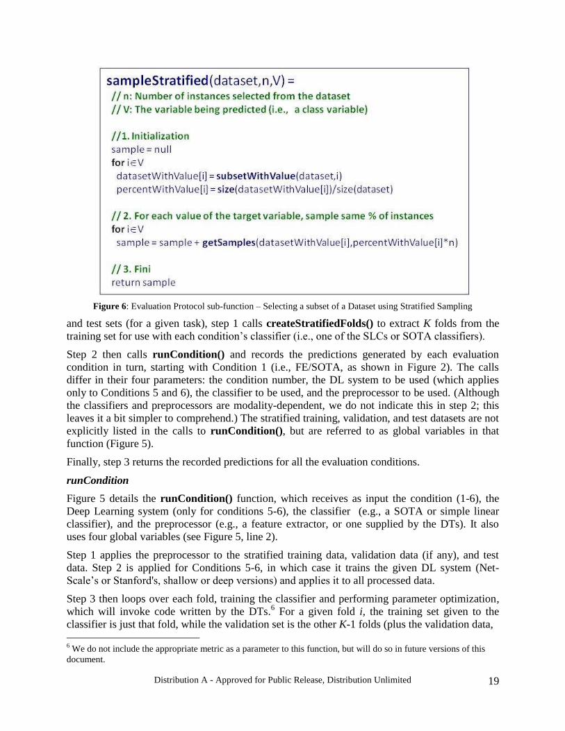
Figure 6: Evaluation Protocol sub-function – Selecting a subset of a Dataset using Stratified Sampling

and test sets (for a given task), step 1 calls createStratifiedFolds() to extract K folds from the

training set for use with each condition’s classifier (i.e., one of the SLCs or SOTA classifiers).

Step 2 then calls runCondition() and records the predictions generated by each evaluation

condition in turn, starting with Condition 1 (i.e., FE/SOTA, as shown in Figure 2). The calls

differ in their four parameters: the condition number, the DL system to be used (which applies

only to Conditions 5 and 6), the classifier to be used, and the preprocessor to be used. (Although

the classifiers and preprocessors are modality-dependent, we do not indicate this in step 2; this

leaves it a bit simpler to comprehend.) The stratified training, validation, and test datasets are not

explicitly listed in the calls to runCondition(), but are referred to as global variables in that

function (Figure 5).

Finally, step 3 returns the recorded predictions for all the evaluation conditions.

runCondition

Figure 5 details the runCondition() function, which receives as input the condition (1-6), the

Deep Learning system (only for conditions 5-6), the classifier (e.g., a SOTA or simple linear

classifier), and the preprocessor (e.g., a feature extractor, or one supplied by the DTs). It also

uses four global variables (see Figure 5, line 2).

Step 1 applies the preprocessor to the stratified training data, validation data (if any), and test

data. Step 2 is applied for Conditions 5-6, in which case it trains the given DL system (Net-

Scale’s or Stanford's, shallow or deep versions) and applies it to all processed data.

Step 3 then loops over each fold, training the classifier and performing parameter optimization,

which will invoke code written by the DTs.6 For a given fold i, the training set given to the

classifier is just that fold, while the validation set is the other K-1 folds (plus the validation data,

6 We do not include the appropriate metric as a parameter to this function, but will do so in future versions of this

document.


20

Figure 7: Evaluation Protocol sub-function – Creating a set of K Stratified Folds for a given Data Set

for the text modality evaluations). It then applies the learned classifier to the test data and records

the predictions for the current fold.

Finally, in step 4 the predictions for all the folds are returned.

Subfunctions

The two sub-functions involved with stratified sampling are shown in Figures 6 and 7. The

sampleStratified() function is shown in Figure 6; it is called twice in runProtocol() (Figure 3).

It takes as input a dataset, the number of instances to sample from that dataset (without

replacement), and the variable whose value is being predicted (i.e., the class variable). The first,

initialization step includes partitioning the dataset into one subset per class, and computing the

percentage of dataset instances per class. Step 2 then extracts samples of the dataset such that its

class distribution mimics the class distribution of the entire dataset. Step 3 returns this sample.

Finally, Figure 7 displays the pseudocode of createStratifiedFolds() for extracting a set of K

stratified folds from a given set of data. This works by ordering the data’s instances by

increasing concept frequency, and then sequentially assigning each (ordered) instance to a fold.

However, it must account for the fact that the instances/clips in the video modality dataset

(Hollywood2) can belong to multiple classes. Although not shown in Figure 7, we will define

orderByIncreasingConceptFrequency() to arbitrarily select the first label associated with each

instance.

Notes

Some of the combined pseudocode’s sub-functions are not shown (e.g., DLSystem(),

getSamples()). However, these figures should provide sufficient detail for the DTs to review.

The most recent change to this section pertains to the selection of the value for N; few other

changes have been made. However, we welcome their recommendations for any additional

changes, although we require agreement from both teams before considering any such

recommendations.


21

5.6 Analysis Procedures

We will conduct a similar analysis for each performance task, although the two tasks will employ

different metrics (average 11-pt precision and RMSE, respectively). In particular, let C be the

number of classes in the task (i.e., 12 for the video modality task and 5 for the text modality

task). We assume K (the number of folds) is the same for each task. Then a classifier (a SLC or

SOTA shallow classifier, depending on the condition) will be trained K times per class,

producing K*|C| metric values as output. Our first graph (per task) will display these by plotting

the metric values for each class.

As explained in §5.4.1, we will compute the average values of these metrics across classes, thus

producing one MAP or mRMSE value per fold. Our second graph will display these by plotting

these per fold, along with their standard errors across the classes.

Finally, we will compute the means of these across the folds, yielding one mean MAP or mean

mRMSE value per performance task. In our third graph, we will plot this value and its standard

error across the folds.

We will rank the results of the two teams’ systems according to their mean MAP (for video

modality) or mean mRMSE value (for text modality), and also note whether their standard errors

suggest significant differences exist between these values for a given performance task.

We welcome feedback from the DTs on the selection of these procedures.

6 Logistics

The ET plans to conduct the evaluation at NRL in such a way that the evaluation can be

replicated simultaneously by the DTs at their respective locations. To do this, we are creating a

test harness that, once integrated with a DL system, can be used to run the evaluation protocols

(§5.5) and the analysis procedures (§5.6). If the results of the ET and a DT differ substantially,

then we will iterate with that DT to determine the cause, with the goal of eliminating it in a

subsequent iteration. The video modality training and test sets for mid-Phase 1 have already been

provided to the DTs. However, the training/test partitions for the text modality dataset have not

been provided, nor the K folds for either modality. These will be provided by the ET to the DTs

soon after the mid-Phase 1 evaluation time period begins.

6.1 Hardware

The ET obtained hardware specifications from both Net-Scale and Stanford. We ordered

machines whose specifications are comparable (e.g., it has 12 GPUs and 36 CPUs). Some details

include:

Power Estimate:

o Watts: 1544.4, Volt-Amps: 1583.01, BTU/h: 5269.49, Amps(110V): 14.04,

Amps(208V): 7.43

Supermicro SuperServer 7046GT-TRF - 6(+2) x SATA - 12 x DDR3 - 1400W

2 x Six-Core Intel® Xeon® X5650 2.66GHz 6.4GT/s QPI 12MB L3 Cache (95W)

12 x 8GB PC3-10600 1333MHz DDR3 ECC Registered

1TB SATA 7200RPM - 3.5" - Seagate Barracuda® ES.2

PNY NVIDIA Quadro FX 380 256MB GDDR3 PCI Express (2xDVI)


22

4 x NVIDIA GeForce GTX 480 1536MB GDDR5 PCI Express 2.0 (2xDVI, 1xmini

HDMI)

We will use this cluster for (1) our Guinea Pig study and (2) for training and testing the DTs’ DL

systems when conducting the evaluations.

However, contingency plans are needed for potential problems that may arise:

Delayed arrival: The systems were due to arrive by 9/30/10, which is later than we

prefer. Furthermore, they did not arrive until 10/13/10.

Machine locations: Due to ongoing upgrades in our server room, the ET must find other

locations at NRL to house these machines, and we are currently investigating options.7

Delayed Guinea Pig study: The timing of this study has slipped. Our intention was to

complete this prior to starting the mid-Phase 1 evaluations (i.e., so as to identify problems

with the test harness and any aspect of the evaluation process beforehand). Unfortunately,

the code is not yet fully functional.

Insufficient time for training: The amount of time required to train the DL systems may

be prohibitive to conduct the evaluation according to our proposed schedule (§7).

Given this context, we are coordinating with the DTs on the following contingency plans:

We asked the DTs to provide, in addition to their system’s source code, the trained DL

systems (one for each of the two performance tasks). We will seek confirmation that they

were learned using the evaluation protocols described in §5.5.

If we cannot run the evaluations on the ET’s machines in time for the mid-Phase 1

evaluation, then we plan to run the evaluations remotely on the DTs’ machines at their

locations. (We have confirmed this plan with the DTs.)

We do not anticipate similar problems with the Guinea Pig study or use of the GPU machines at

NRL for the end-of-Phase 1 evaluation.

6.2 Software

The ET’s test harness is designed to be as lightweight as possible so that (1) it can run the

evaluation conditions (§5.2) using the protocol (§5.3), (2) apply the analysis procedures (§5.6),

(3) graph the results, and (4) requires a minimal amount of coding to integrate with the DTs’ DL

systems. We will include its graphs in the analysis report to be discussed with the DTs and, once

finalized, given to DARPA. It is coded in Python so that the DTs can examine it, quickly

comprehend it, and propose changes if/as needed. We are currently finalizing the test harness.

The test harness requires a simple API for communicating with each DL system. We have

discussed this at the August 2010 PI meeting, and are collaborating with the DTs to integrate

their DL system code with the test harness.

7 Schedule

This abridged schedule is adapted from the DL Kickoff meeting.

7 Due to their high noise levels and heat output, these GPU machines are not suitable for placement in office space,

and their high power requirements must also be considered in placement decisions.


23

October 15th

, 2010 The ET and DTs complete the integration of the DL systems with the

test harness

November 1st, 2010 Mid-Phase 1 evaluation starts

December 10th

, 2010 ET provides mid-Phase 1 analysis report to DARPA

March 1st, 2011 ET provides end-of-phase datasets to DTs

April 5th

, 2011 DTs provide revised preprocessors and simple linear classifiers to ET

July 1st, 2011 DTs provide source code for the (revised) DL systems

Jul 18th

, 2011 End-of-Phase 1 evaluation starts

October 1st, 2011 ET provides end-of-Phase 1 analysis report(s) to DARPA

8 Questions and Contingency Plans

Concerning the mid-Phase 1 evaluation, we listed some remaining questions and contingency

plans here in the previous version of this document. We give a status report on each below.

8.1 Questions (now all answered)

1. Culling the video performance data set: No longer needed because the metric shifted from

accuracy back to MAP.

2. Text performance task variable settings: In correspondence with the DTs, we have settled

on a value of N=10,000.

3. Open Table cutoff: We have settled on a cutoff for each review; they must each contain at

least 30 characters. See §4.2 for more details.

4. Unspecified information: We have now selected the feature extractor that we will use for

the video performance task (§5.3.5), and the analysis procedures that we will use for the

two performance tasks (§5.6).

5. Net-Scale video performance task decisions: We have now received Net-Scale’s

preprocessor and SLC for the video performance task.

8.2 Contingency Plans

1. Test harness: Unfortunately, it is unclear whether we will complete the Guinea Pig

evaluation prior the mid-Phase 1 evaluation time period. However, we are already

interacting with the DTs on integrating the test harness with their DL systems (and other

modules), and we will iterate with them until we are confident that the test harness is

working properly.

2. ET hardware: While the ET has received the GPU machines needed for conducting the

evaluations in-house, we have not finalized their hosting location at NRL. While we are

solving this problem, our contingency plan is to access the DTs’ machines to conduct the

mid-Phase 1 evaluation.

3. Training duration: It is possible that the time required for training the DL systems will be

prohibitive on the ET’s GPU machines. Given this, the DTs are providing both untrained

and trained DL systems for both performance tasks. Thus, if the training process takes too

long, the ET will use the trained DL systems for the evaluation.


24

Acknowledgements

Thanks to DARPA for funding this work, and to all DL program participants who have provided

feedback/comments on, or otherwise contributed to, drafts of this document. Thanks also to Julie

Fitzgerald, who introduced to us the value of detailing a broad evaluation plan. The views and

opinions contained in this paper are those of the authors and should not be interpreted as

representing the official views or policies, either expressed or implied, of NRL, DARPA, or the

Department of Defense.

References

Aha, D.W., & Schneider, A. (2010). Proposal for video dataset selection in DL phase 1. Unpublished.

Blei, D.M., Ng, A., & Jordan, M. (2003). Latent dirichlet allocation. Journal of Machine Learning

Research, 3, 993-1022.

DARPA (2009). Deep Learning (DL) Broad Agency Announcement 09-40. Retrieved on 15 October

2010 from [http://www.darpa.mil/ipto/solicit/baa/BAA-09-40_PIP.pdf].

Schneider, A., & Aha, D.W. (2010). Proposal for text dataset selection in DL phase 1. Unpublished.

Snyder, B., & Barzilay, R. (2007). Multiple aspect ranking using the Good Grief algorithm. Proceedings

of Human Language Technologies: The Annual Conference of the North American Chapter of the

Association for Computational Linguistics (pp. 300-307). Rochester, NY:

ACL. [http://acl.ldc.upenn.edu/N/N07/N07-1038.pdf]

Taylor, G.W., & Bregler, C. (2010). Learning local spatio-temporal features for activity recognition. In

Proceedings of the Snowbird Workshop. Snowbird, Utah. [http://snowbird.djvuzone.org/]

Wang, H., Ullah, M., Kläser, A., Laptev, I., & Schmid, C. (2009). Evaluation of local spatio-temporal

features for action recognition. Proceedings of the British Machine Vision Conference (pp. 127-138).

London. [http://www.bmva.org/bmvc/2009/index.htm]

Yang, Y., & Pedersen, J.O. (1997). A comparative study on feature selection in text categorization.

Proceedings of the Fourteenth International Conference on Machine Learning (pp. 412-420).

Nashville, TN: Morgan Kaufmann.

The DARPA Deep Learning Program’s Broad Evaluation · PDF file3 EVALUATION PROCESS AND...

Documents

Transcript of The DARPA Deep Learning Program’s Broad Evaluation · PDF file3 EVALUATION PROCESS AND...