The Dao of Functional Programming

The Dao of Functional Programming

Bartosz Milewski

(Last updated: February 16, 2022)

Contents

Preface . . . . . . . . . . . . . . . . . . . . . . . . . . . . . . . . . . . . . . . viiiConventions . . . . . . . . . . . . . . . . . . . . . . . . . . . . . . . . . . viii

1 Clean Slate 11.1 Types and Functions . . . . . . . . . . . . . . . . . . . . . . . . . . . . . 11.2 Yin and Yang . . . . . . . . . . . . . . . . . . . . . . . . . . . . . . . . . 21.3 Elements . . . . . . . . . . . . . . . . . . . . . . . . . . . . . . . . . . . 31.4 The Object of Arrows . . . . . . . . . . . . . . . . . . . . . . . . . . . . 4

2 Composition 52.1 Composition . . . . . . . . . . . . . . . . . . . . . . . . . . . . . . . . . 52.2 Function application . . . . . . . . . . . . . . . . . . . . . . . . . . . . . 72.3 Identity . . . . . . . . . . . . . . . . . . . . . . . . . . . . . . . . . . . . 8

3 Isomorphisms 113.1 Isomorphic Objects . . . . . . . . . . . . . . . . . . . . . . . . . . . . . . 113.2 Naturality . . . . . . . . . . . . . . . . . . . . . . . . . . . . . . . . . . . 133.3 Reasoning with Arrows . . . . . . . . . . . . . . . . . . . . . . . . . . . . 14

Reversing the Arrows . . . . . . . . . . . . . . . . . . . . . . . . . . . . 16

i

ii CONTENTS

4 Sum Types 19

4.1 Bool . . . . . . . . . . . . . . . . . . . . . . . . . . . . . . . . . . . . . . 19

Examples . . . . . . . . . . . . . . . . . . . . . . . . . . . . . . . . . . . 21

4.2 Enumerations . . . . . . . . . . . . . . . . . . . . . . . . . . . . . . . . . 22

Short Haskell Digression . . . . . . . . . . . . . . . . . . . . . . . . . . . 23

4.3 Sum Types . . . . . . . . . . . . . . . . . . . . . . . . . . . . . . . . . . 24

Maybe . . . . . . . . . . . . . . . . . . . . . . . . . . . . . . . . . . . . . 25

Logic . . . . . . . . . . . . . . . . . . . . . . . . . . . . . . . . . . . . . . 26

4.4 Cocartesian Categories . . . . . . . . . . . . . . . . . . . . . . . . . . . . 26

One Plus Zero . . . . . . . . . . . . . . . . . . . . . . . . . . . . . . . . . 26

Something Plus Zero . . . . . . . . . . . . . . . . . . . . . . . . . . . . . 27

Commutativity . . . . . . . . . . . . . . . . . . . . . . . . . . . . . . . . 27

Associativity . . . . . . . . . . . . . . . . . . . . . . . . . . . . . . . . . 28

Functoriality . . . . . . . . . . . . . . . . . . . . . . . . . . . . . . . . . 29

Symmetric Monoidal Category . . . . . . . . . . . . . . . . . . . . . . . 29

5 Product Types 31

Logic . . . . . . . . . . . . . . . . . . . . . . . . . . . . . . . . . . . . . . 32

Tuples and Records . . . . . . . . . . . . . . . . . . . . . . . . . . . . . . 32

5.1 Cartesian Category . . . . . . . . . . . . . . . . . . . . . . . . . . . . . . 33

Tuple Arithmetic . . . . . . . . . . . . . . . . . . . . . . . . . . . . . . . 33

Functoriality . . . . . . . . . . . . . . . . . . . . . . . . . . . . . . . . . 35

5.2 Duality . . . . . . . . . . . . . . . . . . . . . . . . . . . . . . . . . . . . 35

5.3 Monoidal Category . . . . . . . . . . . . . . . . . . . . . . . . . . . . . . 36

Monoids . . . . . . . . . . . . . . . . . . . . . . . . . . . . . . . . . . . . 37

6 Function Types 39

Elimination rule . . . . . . . . . . . . . . . . . . . . . . . . . . . . . . . 39

Introduction rule . . . . . . . . . . . . . . . . . . . . . . . . . . . . . . . 40

Currying . . . . . . . . . . . . . . . . . . . . . . . . . . . . . . . . . . . . 41

Relation to lambda calculus . . . . . . . . . . . . . . . . . . . . . . . . . 42

Modus ponens . . . . . . . . . . . . . . . . . . . . . . . . . . . . . . . . 43

6.1 Sum and Product Revisited . . . . . . . . . . . . . . . . . . . . . . . . . 43

Sum types . . . . . . . . . . . . . . . . . . . . . . . . . . . . . . . . . . . 44

Product types . . . . . . . . . . . . . . . . . . . . . . . . . . . . . . . . . 45

Functoriality revisited . . . . . . . . . . . . . . . . . . . . . . . . . . . . 45

6.2 Functoriality of the Function Type . . . . . . . . . . . . . . . . . . . . . 46

6.3 Bicartesian Closed Categories . . . . . . . . . . . . . . . . . . . . . . . . 47

Distributivity . . . . . . . . . . . . . . . . . . . . . . . . . . . . . . . . . 47

7 Recursion 51

7.1 Natural Numbers . . . . . . . . . . . . . . . . . . . . . . . . . . . . . . . 51

Introduction Rules . . . . . . . . . . . . . . . . . . . . . . . . . . . . . . 52

Elimination Rules . . . . . . . . . . . . . . . . . . . . . . . . . . . . . . 52

In Programming . . . . . . . . . . . . . . . . . . . . . . . . . . . . . . . 54

7.2 Lists . . . . . . . . . . . . . . . . . . . . . . . . . . . . . . . . . . . . . . 55

Elimination Rule . . . . . . . . . . . . . . . . . . . . . . . . . . . . . . . 55

7.3 Functoriality . . . . . . . . . . . . . . . . . . . . . . . . . . . . . . . . . 56

CONTENTS iii

8 Functors 59

8.1 Categories . . . . . . . . . . . . . . . . . . . . . . . . . . . . . . . . . . . 59

Category of sets . . . . . . . . . . . . . . . . . . . . . . . . . . . . . . . . 59

Opposite and product categories . . . . . . . . . . . . . . . . . . . . . . 60

8.2 Functors . . . . . . . . . . . . . . . . . . . . . . . . . . . . . . . . . . . . 60

Functors between categories . . . . . . . . . . . . . . . . . . . . . . . . . 61

8.3 Functors in Programming . . . . . . . . . . . . . . . . . . . . . . . . . . 63

Endofunctors . . . . . . . . . . . . . . . . . . . . . . . . . . . . . . . . . 63

Bifunctors . . . . . . . . . . . . . . . . . . . . . . . . . . . . . . . . . . . 64

Profunctors . . . . . . . . . . . . . . . . . . . . . . . . . . . . . . . . . . 65

Contravariant functors . . . . . . . . . . . . . . . . . . . . . . . . . . . . 65

8.4 The Hom-Functor . . . . . . . . . . . . . . . . . . . . . . . . . . . . . . 66

8.5 Functor Composition . . . . . . . . . . . . . . . . . . . . . . . . . . . . . 67

Category of categories . . . . . . . . . . . . . . . . . . . . . . . . . . . . 68

9 Natural Transformations 69

9.1 Natural Transformations Between Hom-Functors . . . . . . . . . . . . . 69

9.2 Natural Transformation Between Functors . . . . . . . . . . . . . . . . . 71

9.3 Natural Transformations in Programming . . . . . . . . . . . . . . . . . 72

9.4 The Functor Category . . . . . . . . . . . . . . . . . . . . . . . . . . . . 73

Vertical composition of natural transformations . . . . . . . . . . . . . . 73

Horizontal composition of natural transformations . . . . . . . . . . . . 75

Whiskering . . . . . . . . . . . . . . . . . . . . . . . . . . . . . . . . . . 76

Interchange law . . . . . . . . . . . . . . . . . . . . . . . . . . . . . . . . 77

9.5 Universal Constructions Revisited . . . . . . . . . . . . . . . . . . . . . 77

Picking objects . . . . . . . . . . . . . . . . . . . . . . . . . . . . . . . . 78

Cospans as natural transformations . . . . . . . . . . . . . . . . . . . . . 78

Functoriality of cospans . . . . . . . . . . . . . . . . . . . . . . . . . . . 79

Sum as a universal cospan . . . . . . . . . . . . . . . . . . . . . . . . . . 80

Product as a universal span . . . . . . . . . . . . . . . . . . . . . . . . . 81

Exponentials . . . . . . . . . . . . . . . . . . . . . . . . . . . . . . . . . 81

9.6 Limits and Colimits . . . . . . . . . . . . . . . . . . . . . . . . . . . . . 84

9.7 The Yoneda Lemma . . . . . . . . . . . . . . . . . . . . . . . . . . . . . 85

Yoneda lemma in programming . . . . . . . . . . . . . . . . . . . . . . . 86

The contravariant Yoneda lemma . . . . . . . . . . . . . . . . . . . . . . 87

9.8 Yoneda Embedding . . . . . . . . . . . . . . . . . . . . . . . . . . . . . . 87

9.9 Representable Functors . . . . . . . . . . . . . . . . . . . . . . . . . . . 89

The guessing game . . . . . . . . . . . . . . . . . . . . . . . . . . . . . . 90

Representable functors in programming . . . . . . . . . . . . . . . . . . 90

9.10 2-category Cat . . . . . . . . . . . . . . . . . . . . . . . . . . . . . . . . 91

10 Adjunctions 93

10.1 The Currying Adjunction . . . . . . . . . . . . . . . . . . . . . . . . . . 93

10.2 The Sum and the Product Adjunctions . . . . . . . . . . . . . . . . . . . 94

The diagonal functor . . . . . . . . . . . . . . . . . . . . . . . . . . . . . 94

The sum adjunction . . . . . . . . . . . . . . . . . . . . . . . . . . . . . 94

The product adjunction . . . . . . . . . . . . . . . . . . . . . . . . . . . 95

10.3 Adjunction between functors . . . . . . . . . . . . . . . . . . . . . . . . 96

iv CONTENTS

10.4 Limits and Colimits . . . . . . . . . . . . . . . . . . . . . . . . . . . . . 97

10.5 Unit and Counit of Adjunction . . . . . . . . . . . . . . . . . . . . . . . 98

Triangle identities . . . . . . . . . . . . . . . . . . . . . . . . . . . . . . 99

The unit and counit of the currying adjunction . . . . . . . . . . . . . . 100

10.6 Distributivity . . . . . . . . . . . . . . . . . . . . . . . . . . . . . . . . . 101

10.7 Free-Forgetful Adjunctions . . . . . . . . . . . . . . . . . . . . . . . . . . 102

The category of monoids . . . . . . . . . . . . . . . . . . . . . . . . . . . 102

Free monoid . . . . . . . . . . . . . . . . . . . . . . . . . . . . . . . . . . 103

Free monoid in programming . . . . . . . . . . . . . . . . . . . . . . . . 104

10.8 The Category of Adjunctions . . . . . . . . . . . . . . . . . . . . . . . . 105

10.9 Levels of Abstraction . . . . . . . . . . . . . . . . . . . . . . . . . . . . . 106

11 Dependent Types 107

11.1 Dependent Vectors . . . . . . . . . . . . . . . . . . . . . . . . . . . . . . 107

11.2 Dependent Types Categorically . . . . . . . . . . . . . . . . . . . . . . . 109

Fibrations . . . . . . . . . . . . . . . . . . . . . . . . . . . . . . . . . . . 109

Type families as fibrations . . . . . . . . . . . . . . . . . . . . . . . . . . 110

Slice categories . . . . . . . . . . . . . . . . . . . . . . . . . . . . . . . . 110

Coslice categories . . . . . . . . . . . . . . . . . . . . . . . . . . . . . . . 110

Pullbacks . . . . . . . . . . . . . . . . . . . . . . . . . . . . . . . . . . . 111

Base-change functor . . . . . . . . . . . . . . . . . . . . . . . . . . . . . 113

11.3 Dependent Sum . . . . . . . . . . . . . . . . . . . . . . . . . . . . . . . . 114

Existential quantification . . . . . . . . . . . . . . . . . . . . . . . . . . 116

11.4 Dependent Product . . . . . . . . . . . . . . . . . . . . . . . . . . . . . . 117

Dependent product in Haskell . . . . . . . . . . . . . . . . . . . . . . . . 117

Dependent product of sets . . . . . . . . . . . . . . . . . . . . . . . . . . 117

Dependent product categorically . . . . . . . . . . . . . . . . . . . . . . 117

Universal quantification . . . . . . . . . . . . . . . . . . . . . . . . . . . 121

11.5 Equality . . . . . . . . . . . . . . . . . . . . . . . . . . . . . . . . . . . . 121

Equational reasoning . . . . . . . . . . . . . . . . . . . . . . . . . . . . . 122

Equality vs isomorphism . . . . . . . . . . . . . . . . . . . . . . . . . . . 123

Equality types . . . . . . . . . . . . . . . . . . . . . . . . . . . . . . . . 124

Introduction rule . . . . . . . . . . . . . . . . . . . . . . . . . . . . . . . 124

β-reduction and η-conversion . . . . . . . . . . . . . . . . . . . . . . . . 124

Induction principle for natural numbers . . . . . . . . . . . . . . . . . . 125

Equality elimination rule . . . . . . . . . . . . . . . . . . . . . . . . . . . 126

12 Algebras 129

12.1 Algebras from Endofunctors . . . . . . . . . . . . . . . . . . . . . . . . . 130

12.2 Category of Algebras . . . . . . . . . . . . . . . . . . . . . . . . . . . . . 131

Initial algebra . . . . . . . . . . . . . . . . . . . . . . . . . . . . . . . . . 131

12.3 Lambek’s Lemma and Fixed Points . . . . . . . . . . . . . . . . . . . . . 132

Fixed point in Haskell . . . . . . . . . . . . . . . . . . . . . . . . . . . . 133

12.4 Catamorphisms . . . . . . . . . . . . . . . . . . . . . . . . . . . . . . . . 134

Examples . . . . . . . . . . . . . . . . . . . . . . . . . . . . . . . . . . . 135

Lists as initial algebras . . . . . . . . . . . . . . . . . . . . . . . . . . . . 136

12.5 Initial Algebra from Universality . . . . . . . . . . . . . . . . . . . . . . 137

12.6 Initial Algebra as a Colimit . . . . . . . . . . . . . . . . . . . . . . . . . 138

CONTENTS v

13 Coalgebras 143

13.1 Coalgebras from Endofunctors . . . . . . . . . . . . . . . . . . . . . . . 143

13.2 Category of Coalgebras . . . . . . . . . . . . . . . . . . . . . . . . . . . 144

13.3 Anamorphisms . . . . . . . . . . . . . . . . . . . . . . . . . . . . . . . . 146

Infinite data structures . . . . . . . . . . . . . . . . . . . . . . . . . . . . 146

13.4 Hylomorphisms . . . . . . . . . . . . . . . . . . . . . . . . . . . . . . . . 147

The impedance mismatch . . . . . . . . . . . . . . . . . . . . . . . . . . 148

13.5 Terminal Coalgebra from Universality . . . . . . . . . . . . . . . . . . . 149

13.6 Terminal Coalgebra as a Limit . . . . . . . . . . . . . . . . . . . . . . . 150

14 Monads 153

14.1 Programming with Side Effects . . . . . . . . . . . . . . . . . . . . . . . 153

Partiality . . . . . . . . . . . . . . . . . . . . . . . . . . . . . . . . . . . 154

Logging . . . . . . . . . . . . . . . . . . . . . . . . . . . . . . . . . . . . 154

Environment . . . . . . . . . . . . . . . . . . . . . . . . . . . . . . . . . 154

State . . . . . . . . . . . . . . . . . . . . . . . . . . . . . . . . . . . . . . 155

Nondeterminism . . . . . . . . . . . . . . . . . . . . . . . . . . . . . . . 155

Input/Output . . . . . . . . . . . . . . . . . . . . . . . . . . . . . . . . . 156

Continuation . . . . . . . . . . . . . . . . . . . . . . . . . . . . . . . . . 156

14.2 Composing Effects . . . . . . . . . . . . . . . . . . . . . . . . . . . . . . 157

14.3 Alternative Definitions . . . . . . . . . . . . . . . . . . . . . . . . . . . . 158

14.4 Monad Instances . . . . . . . . . . . . . . . . . . . . . . . . . . . . . . . 160

Partiality . . . . . . . . . . . . . . . . . . . . . . . . . . . . . . . . . . . 160

Logging . . . . . . . . . . . . . . . . . . . . . . . . . . . . . . . . . . . . 160

Environment . . . . . . . . . . . . . . . . . . . . . . . . . . . . . . . . . 161

State . . . . . . . . . . . . . . . . . . . . . . . . . . . . . . . . . . . . . . 161

Nondeterminism . . . . . . . . . . . . . . . . . . . . . . . . . . . . . . . 162

Continuation . . . . . . . . . . . . . . . . . . . . . . . . . . . . . . . . . 162

Input/Output . . . . . . . . . . . . . . . . . . . . . . . . . . . . . . . . . 163

14.5 Do Notation . . . . . . . . . . . . . . . . . . . . . . . . . . . . . . . . . . 163

14.6 Monads Categorically . . . . . . . . . . . . . . . . . . . . . . . . . . . . 165

Substitution . . . . . . . . . . . . . . . . . . . . . . . . . . . . . . . . . . 165

Monad as a monoid . . . . . . . . . . . . . . . . . . . . . . . . . . . . . 165

14.7 Free Monads . . . . . . . . . . . . . . . . . . . . . . . . . . . . . . . . . 167

Category of monads . . . . . . . . . . . . . . . . . . . . . . . . . . . . . 167

Free monad . . . . . . . . . . . . . . . . . . . . . . . . . . . . . . . . . . 168

Stack calculator example . . . . . . . . . . . . . . . . . . . . . . . . . . . 170

14.8 Monoidal Functors . . . . . . . . . . . . . . . . . . . . . . . . . . . . . . 172

Lax monoidal functors . . . . . . . . . . . . . . . . . . . . . . . . . . . . 173

Functorial strength . . . . . . . . . . . . . . . . . . . . . . . . . . . . . . 174

Applicative functors . . . . . . . . . . . . . . . . . . . . . . . . . . . . . 175

Closed functors . . . . . . . . . . . . . . . . . . . . . . . . . . . . . . . . 176

Monads and applicatives . . . . . . . . . . . . . . . . . . . . . . . . . . . 177

15 Monads from Adjunctions 179

15.1 String Diagrams . . . . . . . . . . . . . . . . . . . . . . . . . . . . . . . 179

String diagrams for the monad . . . . . . . . . . . . . . . . . . . . . . . 181

String diagrams for the adjunction . . . . . . . . . . . . . . . . . . . . . 183

vi CONTENTS

15.2 Monads from Adjunctions . . . . . . . . . . . . . . . . . . . . . . . . . . 184

15.3 Examples of Monads from Adjunctions . . . . . . . . . . . . . . . . . . . 185

Free monoid and the list monad . . . . . . . . . . . . . . . . . . . . . . . 185

The currying adjunction and the state monad . . . . . . . . . . . . . . . 186

M-sets and the writer monad . . . . . . . . . . . . . . . . . . . . . . . . 188

Pointed objects and the Maybe monad . . . . . . . . . . . . . . . . . . . 189

The continuation monad . . . . . . . . . . . . . . . . . . . . . . . . . . . 190

15.4 Monad Transformers . . . . . . . . . . . . . . . . . . . . . . . . . . . . . 190

15.5 Monad Algebras . . . . . . . . . . . . . . . . . . . . . . . . . . . . . . . 193

Eilenberg-Moore category . . . . . . . . . . . . . . . . . . . . . . . . . . 194

Kleisli category . . . . . . . . . . . . . . . . . . . . . . . . . . . . . . . . 195

16 Comonads 197

16.1 Comonads in Programming . . . . . . . . . . . . . . . . . . . . . . . . . 197

The Stream comonad . . . . . . . . . . . . . . . . . . . . . . . . . . . . 198

16.2 Comonads Categorically . . . . . . . . . . . . . . . . . . . . . . . . . . . 199

Comonoids . . . . . . . . . . . . . . . . . . . . . . . . . . . . . . . . . . 200

16.3 Comonads from Adjunctions . . . . . . . . . . . . . . . . . . . . . . . . 201

Costate comonad . . . . . . . . . . . . . . . . . . . . . . . . . . . . . . . 202

Comonad coalgebras . . . . . . . . . . . . . . . . . . . . . . . . . . . . . 204

Lenses . . . . . . . . . . . . . . . . . . . . . . . . . . . . . . . . . . . . . 204

17 Ends and Coends 207

17.1 Profunctors . . . . . . . . . . . . . . . . . . . . . . . . . . . . . . . . . . 207

Collages . . . . . . . . . . . . . . . . . . . . . . . . . . . . . . . . . . . . 208

Profunctors as relations . . . . . . . . . . . . . . . . . . . . . . . . . . . 208

Profunctor composition in Haskell . . . . . . . . . . . . . . . . . . . . . 209

17.2 Coends . . . . . . . . . . . . . . . . . . . . . . . . . . . . . . . . . . . . 210

Profunctor composition using coends . . . . . . . . . . . . . . . . . . . . 212

17.3 Ends . . . . . . . . . . . . . . . . . . . . . . . . . . . . . . . . . . . . . . 213

Natural transformations as an end . . . . . . . . . . . . . . . . . . . . . 215

17.4 Continuity of the Hom-Functor . . . . . . . . . . . . . . . . . . . . . . . 216

17.5 Ninja Yoneda Lemma . . . . . . . . . . . . . . . . . . . . . . . . . . . . 217

Yoneda lemma in Haskell . . . . . . . . . . . . . . . . . . . . . . . . . . 219

17.6 Day Convolution . . . . . . . . . . . . . . . . . . . . . . . . . . . . . . . 219

Applicative functors as monoids . . . . . . . . . . . . . . . . . . . . . . . 220

Free Applicatives . . . . . . . . . . . . . . . . . . . . . . . . . . . . . . . 221

17.7 The Bicategory of Profunctors . . . . . . . . . . . . . . . . . . . . . . . 223

Monads in a bicategory . . . . . . . . . . . . . . . . . . . . . . . . . . . 224

Prearrows as monads in Prof . . . . . . . . . . . . . . . . . . . . . . . . 224

17.8 Existential Lens . . . . . . . . . . . . . . . . . . . . . . . . . . . . . . . . 225

Existential lens in Haskell . . . . . . . . . . . . . . . . . . . . . . . . . . 225

Existential lens in category theory . . . . . . . . . . . . . . . . . . . . . 226

Type-changing lens in Haskell . . . . . . . . . . . . . . . . . . . . . . . . 227

Lens composition . . . . . . . . . . . . . . . . . . . . . . . . . . . . . . . 227

Category of lenses . . . . . . . . . . . . . . . . . . . . . . . . . . . . . . 228

17.9 Lenses and Fibrations . . . . . . . . . . . . . . . . . . . . . . . . . . . . 229

Transport law . . . . . . . . . . . . . . . . . . . . . . . . . . . . . . . . . 229

CONTENTS vii

Identity law . . . . . . . . . . . . . . . . . . . . . . . . . . . . . . . . . . 230Composition law . . . . . . . . . . . . . . . . . . . . . . . . . . . . . . . 230Type-changing lens . . . . . . . . . . . . . . . . . . . . . . . . . . . . . . 231

17.10Important Formulas . . . . . . . . . . . . . . . . . . . . . . . . . . . . . 231

18 Tambara Modules 23318.1 Tannakian Reconstruction . . . . . . . . . . . . . . . . . . . . . . . . . . 233

Monoids and their Representations . . . . . . . . . . . . . . . . . . . . . 233Tannakian reconstruction of a monoid . . . . . . . . . . . . . . . . . . . 234Cayley’s theorem . . . . . . . . . . . . . . . . . . . . . . . . . . . . . . . 236Proof of Tannakian reconstruction . . . . . . . . . . . . . . . . . . . . . 238Tannakian reconstruction in Haskell . . . . . . . . . . . . . . . . . . . . 239Pointed getter . . . . . . . . . . . . . . . . . . . . . . . . . . . . . . . . . 240Tannakian reconstruction with adjunction . . . . . . . . . . . . . . . . . 241

18.2 Profunctor Lenses . . . . . . . . . . . . . . . . . . . . . . . . . . . . . . 243Iso . . . . . . . . . . . . . . . . . . . . . . . . . . . . . . . . . . . . . . . 243Profunctors and lenses . . . . . . . . . . . . . . . . . . . . . . . . . . . . 244Tambara module . . . . . . . . . . . . . . . . . . . . . . . . . . . . . . . 244Profunctor lenses . . . . . . . . . . . . . . . . . . . . . . . . . . . . . . . 246Profunctor lenses in Haskell . . . . . . . . . . . . . . . . . . . . . . . . . 247

18.3 General Optics . . . . . . . . . . . . . . . . . . . . . . . . . . . . . . . . 248Prisms . . . . . . . . . . . . . . . . . . . . . . . . . . . . . . . . . . . . . 248Traversals . . . . . . . . . . . . . . . . . . . . . . . . . . . . . . . . . . . 249

18.4 General Optics . . . . . . . . . . . . . . . . . . . . . . . . . . . . . . . . 251

Index 253

viii CONTENTS

Preface

Most programming texts, following Brian Kernighan, start with ”Hello World!”. It’snatural to want to get the immediate gratification of making the computer do yourbidding and print these famous words. But the real mastery of computer programminggoes deeper than that, and rushing into it may only give you a false feeling of power,when in reality you’re just parroting the masters. If your ambition is just to learn auseful, well-paid skill then, by all means, write your ”Hello World!” program. Thereare tons of books and courses that will teach you to write code in any language of yourchoice. However, if you really want to get to the essence of programming, you need tobe patient and persistent.

Conventions

I tried to keep the notation coherent throughout the book. In particular, I decided touse lowercase letters like a or b for objects in a category and uppercase names like Sfor sets, even though sets are objects in the category of sets and functions. Genericcategories have names like C or D, whereas specific categories are named like Set orCat.

Programming examples are written in Haskell. Although this is not a Haskell man-ual, the introduction of language constructs is gradual enough to help the reader nav-igate the code. The fact that Haskell syntax is often based on mathematical notationis an additional advantage. Program fragments are written in the following format:

apply :: (a -> b, a) -> b

apply (f, x) = f x

Chapter 1

Clean Slate

Programming starts with types and functions. You probably have some preconceptionsabout what types and functions are: get rid of them! They will cloud your mind.

Don’t think about how things are implemented in hardware. What computers are isjust one of the many models of computation. We shouldn’t get attached to it. You canperform computations in your mind, or with pen and paper. The physical substrate isirrelevant to the idea of programming.

1.1 Types and Functions

Paraphrasing Lao Tzu: The type that can be described is not the eternal type. In otherwords, type is a primitive notion. It cannot be defined.

Instead of calling it a type, we could as well call it an object or a proposition. Theseare the words that are used to describe it in different areas of mathematics (type theory,category theory, and logic, respectively).

There may be more than one type, so we need a way to name them. We could do itby pointing fingers at them, but since we want to effectively communicate with otherpeople, we usually name them. So we’ll talk about type a, b, c; or Int, Bool, Double,and so on. These are just names.

A type by itself has no meaning. What makes it special is how it connects to othertypes. The connections are described by arrows. An arrow has one type as its sourceand one type as its target. The target could be the same as the source, in which casethe arrow loops around.

An arrow between types is called a function. An arrow between objects is calleda morphism. An arrow between propositions is called an entailment. These are justwords that are used to describe arrows in different areas of mathematics. You can usethem interchangeably.

A proposition is something that may be true. In logic, we interpret an arrow betweentwo objects as a entails b, or b is derivable from a.

1

2 CHAPTER 1. CLEAN SLATE

There may be more than one arrow between two types, so we need to name them.For instance, here’s an arrow called f that goes from type a to type b

af−→ b

One way to interpret this is to say that the function f takes an argument of type aand produces a result of type b. Or that f is a proof that if a is true then b is also true.

Note: The connection between type theory, lambda calculus (which is the founda-tion of programming), logic, and category theory is known as Curry-Howard-Lambekcorrespondence.

1.2 Yin and Yang

An object is defined by its connections. An arrow is a proof, a witness, of the fact thattwo objects are connected. Sometimes there’s no proof, the objects are disconnected;sometimes there are many proofs; and sometimes there’s a single proof—a unique arrowbetween two objects.

What does it mean to be unique? It means that if you can find two of those, thenthey must be equal.

An object that has a unique outgoing arrow to every object is called the initialobject.

Its dual is an object that has a unique incoming arrow from every object. It’s calledthe terminal object.

In mathematics, the initial object is often denoted by 0 and the terminal object by1.

The initial object is the source of everything. As a type it’s known, in Haskell, asVoid. It symbolizes the chaos from which everything arises. Since there is an arrowfrom Void to everything, there is also an arrow from Void to itself.

Void

Thus Void begets Void and everything else.

The terminal object unites everything. As a type it’s know as Unit. It symbolizesthe ultimate order.

In logic, the terminal object signifies the ultimate truth, symbolized by T or >. Thefact that there’s an arrow to it from any object means that > is true no matter whatyour assumptions are.

Dually, the initial object signifies logical falsehood, contradiction, or a counterfac-tual. It’s written as False and symbolized by an upside down T, ⊥. The fact that thereis an arrow from it to any object means that you can prove anything starting from falsepremises.

In English, there is special grammatical construct for counterfactual implications.When we say, “If wishes were horses, beggars would ride,” we mean that the equalitybetween wishes and horses implies that beggars be able to ride. But we know that thepremise is false.

1.3. ELEMENTS 3

A programming language lets us communicate with each other and with computers.Some languages are easier for the computer to understand, others are closer to thetheory. We will use Haskell as a compromise.

In Haskell, the initial object corresponds to the type called Void. The name for theterminal type is (), a pair of empty parentheses, pronounced Unit. This notation willmake sense later.

There are infinitely many types in Haskell, and there is a unique function/arrowfrom Void to each one of them. All these functions are known under the same name:absurd.

Programming Category theory Logic

type object propositionfunction morphism (arrow) implicationVoid initial object, 0 False ⊥() terminal object, 1 True >

1.3 Elements

An object has no parts but it may have structure. The structure is defined by thearrows pointing at the object. We can probe the object with arrows.

In programming and in logic we want our initial object to have no structure. Sowe’ll assume that it has no incoming arrows (other than the one that’s looping backfrom it). Therefore Void has no structure.

The terminal object has the simplest structure. There is only one incoming arrowfrom any object to it: there is only one way of probing it from any direction. In thisrespect, the terminal object behaves like an indivisible point. Its only property is thatit exists, and the arrow from any other object proves it.

Because the terminal object is so simple, we can use it to probe other, more complexobjects.

If there is more than one arrow coming from the terminal object to some object a,it means that a has some structure: there is more than one way of looking at it. Sincethe terminal object behaves like a point, we can visualize each arrow from it as pickinga different point or element of its target.

In category theory we say that x is a global element of a if it’s an arrow

1x−→ a

We’ll often simply call it an element (omitting “global”).

In type theory, x : A means that x is of type A.

In Haskell, we use the double-colon notation instead:

x :: A

(Haskell uses capitalized names for concrete types, and lower-cased names for typevariables.)

We say that x is a term of type A but, categorically, we’ll interpret it as an arrowx : 1→ A, a global element of A. 1

1The Haskell type system distinguishes between x :: A and x :: () -> A. However, they denotethe same thing in categorical semantics.

4 CHAPTER 1. CLEAN SLATE

In logic, such x is called the proof of A, since it corresponds to the implication> → A (if True is true then A is true). Notice that there may be many differentproofs of A.

Since we have assumed that there be no arrows from any other object to Void, thereis no arrow from the terminal object to it. Therefore Void has no elements. This iswhy we think of Void as empty.

The terminal object has just one element, since there is a unique arrow coming fromit to itself, 1→ 1. This is why we sometimes call it a singleton.

Note: In category theory there is no prohibition against the initial object havingincoming arrows from other objects. However, in cartesian closed categories that we’restudying here, this is not allowed.

1.4 The Object of Arrows

We describe an object by looking at its arrows. Can we describe an arrow in a similarway? Could an arrow from a to b be represented as an element of some special objectof arrows? After all, in programming we talk about the type of functions from a to b.In Haskell we write:

f :: a -> b

meaning that f is of the type “function from a to b”. Here, a->b is just the name weare giving to this type. To fully define this type, we would have to describe its relationto other objects, in particular to a and b. We don’t have the tools to do that yet, butwe’ll get there.

For now, let’s keep in mind the following distinction: On the one hand we have anarrow which connects two objects a and b. On the other hand we have an element ofthe object of arrows from a to b. This element is itself defined as an arrow from theterminal object () to the object we call a->b.

The notation we use in programming tends to blur this distinction. This is whyin category theory we call the object of arrows an exponential and write it as ba (thesource is in the exponent). So the statement:

f :: a -> b

is equivalent to

1f−→ ba

In logic, an arrow A → B is an implication: it states the fact that “if A then B.”An exponential object BA is the corresponding proposition. It could be true or it couldbe false, we don’t know. You have to prove it. Such a proof is an element of BA.

Show me an element of BA and I’ll know that B follows from A.Consider again the statement, “If wishes were horses, beggars would ride”—this

time as an object. It’s not an empty object, because you can point at a proof of it—something along the lines: “A person who has a horse rides it. Beggars have wishes.Since wishes are horses, beggars have horses. Therefore beggars ride.” But, even thoughyou have a proof of this statement, it’s of no use to you, because you can never proveits premise: “wish = horse”.

Chapter 2

Composition

2.1 Composition

Programming is about composition. Paraphrasing Wittgenstein, one could say: “Ofthat which cannot be decomposed one should not speak.” This is not a prohibition,it’s a statement of fact. The process of studying, understanding, and describing is thesame as the process of decomposing; and our language reflects this.

The reason we have built the vocabulary of objects and arrows is precisely to expressthe idea of composition.

Given an arrow f from a to b and an arrow g from b to c, their composition is anarrow that goes directly from a to c. In other words, if there are two arrows, the targetof one being the same as the source of the other, we can always compose them to get athird arrow.

a b c

h

f g

In math we denote composition using a little circle

h = g ◦ f

We read this: “h is equal to g after f .” The order of composition might seem backward,but this is because we think of functions as taking arguments on the right. In Haskellwe replace the circle with a dot:

h = g . f

This is every program in a nutshell. In order to accomplish h, we decompose it intosimpler problems, f and g. These, in turn, can be decomposed further, and so on.

Now suppose that we were able to decompose g itself into j ◦ k. We have

h = (j ◦ k) ◦ f

We want this decomposition to be the same as

h = j ◦ (k ◦ f)

5

6 CHAPTER 2. COMPOSITION

We want to be able to say that we have decomposed h into three simpler problems

h = j ◦ k ◦ f

and not have to keep track which decomposition came first. This is called associativityof composition, and we will assume it from now on.

Composition is the source of two mappings of arrows called pre-composition andpost-composition.

When an arrow f is post-composed after an arrow h, it produces the arrow f ◦ h.Of course, f can be post-composed only after arrows whose target is the source of f .Post-composition by f is written as (f ◦ −), leaving a hole for h. As Lao Tzu wouldsay, “Usefulness of post-composition comes from what is not there.”

Thus an arrow f : a → b induces a mapping of arrows (f ◦ −) that maps arrowswhich are probing a to arrows which are probing b.

a bf

(f ◦ −)

Since objects have no internal structure, when we say that f transforms a to b, this isexactly what we mean.

Post-composition lets us shift focus from one object to another.Dually, you can pre-compose f , or apply (−◦ f) to arrows originating in b and map

them to arrows originating in a.

a bf

(− ◦ f)

Pre-composition let us shift the perspective from one observer to another. Noticethat the outgoing arrows are mapped in the direction opposite to the shifting arrow f .

Another way of looking at pre- and post-composition is that they are the result ofpartial application of the two-hole composition operator (− ◦ −), in which we pre-fillone hole or the other with an arrow.

In programming, an outgoing arrow is interpreted as extracting data from the source.An incoming arrow is interpreted as producing or constructing the target. Outgoingarrows define the interface, incoming arrows define the constructors.

Do the following exercises to convince yourself that shifts in focus and perspectiveare composable.

Exercise 2.1.1. Suppose that you have two arrows, f : a → b and g : b → c. Theircomposition g ◦ f induces a mapping of arrows ((g ◦ f) ◦−). Show that the result is thesame if you first apply (f ◦ −) and follow it by (g ◦ −). Symbolically:

((g ◦ f) ◦ −) = (g ◦ −) ◦ (f ◦ −)

2.2. FUNCTION APPLICATION 7

Hint: Pick an arbitrary object x and an arrow h : x→ a and see if you get the sameresult.

Exercise 2.1.2. Convince yourself that the composition from the previous exercise isassociative. Hint: Start with three composable arrows.

Exercise 2.1.3. Show that pre-composition (− ◦ f) is composable, but the order ofcomposition is reversed:

(− ◦ (g ◦ f)) = (− ◦ f) ◦ (− ◦ g)

2.2 Function application

We are ready to write our first program. There is a saying: “A journey of a thousandmiles begins with a single step.” Our journey is from 1 to b. The single step is an arrowfrom the terminal object 1 to a. It’s an element of a. We can write it as

1x−→ a

The rest of the journey is the arrow

af−→ b

These two arrows are composable (they share the object a in the middle) and theircomposition is the arrow y from 1 to b. In other words, y is an element of b

1 a b

y

x f

We can write it asy = f ◦ x

We used f to map an element of a to an element of b. Since this is something wedo quite often, we call it the application of a function f to x, and use the shorthandnotation

y = fx

Let’s translate it to Haskell. We start with an element x of a (a shorthand for ()->a)

x :: a

We declare a function f as an element of the “object of arrows” from a to b

f :: a -> b

with the understanding (which will be elaborated upon later) that it corresponds to anarrow from a to b. The result is an element of b

y :: b

and it is defined as

y = f x

We call this the application of a function to an argument, but we were able to expressit purely in terms of function composition. (Note: In other programming languagesfunction application requires the use of parentheses, e.g., y = f(x).)

8 CHAPTER 2. COMPOSITION

2.3 Identity

You may think of arrows as representing change: object a becomes object b. An arrowthat loops back represents a change in an object itself. But change has its dual: lackof change, inaction or, as Lao Tzu would say wu wei.

Every object has a special arrow called the identity, which leaves the object un-changed. It means that, when you compose this arrow with any other arrow, eitherincoming or outgoing, you get that arrow back. Identity arrow does nothing to anarrow.

An identity arrow on the object a is called ida. So if we have an arrow f : a → b,we can compose it with identities on either side

idb ◦ f = f = f ◦ ida

or, pictorially:

a b

ida

f

idb

We can easily check what an identity does to elements. Let’s take an elementx : 1→ a and compose it with ida. The result is:

ida ◦ x = x

which means that identity leaves elements unchanged.

In Haskell, we use the same name id for all identity functions (we don’t subscriptit with the type it’s acting on). The above equation, which specifies the action of id onelements, translates directly to:

id x = x

and it becomes the definition of the function id.

We’ve seen before that both the initial object and the terminal object have uniquearrows circling back to them. Now we are saying that every object has an identity arrowcircling back to it. Remember what we said about uniqueness: If you can find two ofthose, then they must be equal. We must conclude that these unique looping arrowswe talked about must be the identity arrows. We can now label these diagrams:

Void

id

()

id

In logic, identity arrow translates to a tautology. It’s a trivial proof that, “if a istrue then a is true.” It’s also called the identity rule.

If identity does nothing then why do we care about it? Imagine going on a trip,composing a few arrows, and finding yourself back at the starting point. The questionis: Have you done anything, or have you wasted your time? The only way to answerthis question is to compare your path with the identity arrow.

Some round trips bring change, others don’t.

2.3. IDENTITY 9

Exercise 2.3.1. What does (ida◦−) do to arrows terminating in a? What does (−◦ida)do to arrows originating from a?

Chapter 3

Isomorphisms

When we say thatf ◦ (g ◦ h) = (f ◦ g) ◦ h

orf = f ◦ id

we are asserting the equality of arrows. The arrow on the left is the result of oneoperation, and the arrow on the right is the result of another. But the results are equal.

We often illustrate such equalities by drawing commuting diagrams, e.g.,

a b c dh

g◦h

f◦(g◦h)

(f◦g)◦h

g

f◦g

fa b

f

id

Thus we compare arrows for equality.We do not compare objects for equality. We see objects as confluences of arrows,

so if we want to compare two objects, we look at the arrows.

3.1 Isomorphic Objects

The simplest relation between two objects is an arrow.The simplest round trip is a composition of two arrows going in opposite directions.

a b

f

g

There are two possible round trips. One is g ◦ f , which goes from a to a. The otheris f ◦ g , which goes from b to b.

If both of them result in identities, than we say that g is the inverse of f

g ◦ f = idA

11

12 CHAPTER 3. ISOMORPHISMS

f ◦ g = idB

and we write it as g = f−1 (pronounced f inverse). The arrow f−1 undoes the work ofthe arrow f .

Such a pair of arrows is called an isomorphism and the two objects are calledisomorphic.

What does the existence of an isomorphisms tell us about the two objects theyconnect?

We have said that objects are described by their interactions with other objects.So let’s consider what the two isomorphic objects look like from the perspective of anobserver object x. Take an arrow h coming from x to a.

x

a b

h

f

f−1

There is a corresponding arrow coming from x to b. It’s just the composition of f ◦ h,or the action of (f ◦ −) on h.

x

a b

h f◦h

f

f−1

Similarly, for any arrow probing b there is a corresponding arrow probing a. It is givenby the action of (f−1 ◦ −).

We can move focus back and forth between a and b using the mappings (f ◦−) and(f−1 ◦ −).

We can combine these two mappings (see exercise 2.1.1) to form a round trip. Theresult is the same as if we applied the composite ((f−1 ◦ f) ◦ −). But this is equal to(idA ◦ −) which, as we know from exercise 2.3.1, leaves the arrows unchanged.

Similarly, the round trip induced by f ◦ f−1 leaves the arrows x→ b unchanged.

This creates a “buddy system” between the two groups of arrows. Imagine eacharrow sending a message to its buddy, as determined by f or f−1. Each arrow wouldthen receive exactly one message, and that would be a message from its buddy. Noarrow would be left behind, and no arrow would receive more than one message. Math-ematicians call this kind of buddy system a bijection or one-to-one correspondence.

Therefore, arrow by arrow, the two objects a and b look exactly the same from theperspective of x. Arrow-wise, there is no difference between the two objects.

In particular, if you replace x with the terminal object 1, you’ll see that the twoobjects have the same elements. For every element x : 1 → a there is a correspondingelement y : 1 → b, namely y = f ◦ x, and vice versa. There is a bijection between theelements of isomorphic objects.

Such indistinguishable objects are called isomorphic because they have “the sameshape.” You’ve seen one, you’ve seen them all.

We write this isomorphism as:

3.2. NATURALITY 13

a ∼= b

When dealing with objects, we use isomorphism in place of equality.

In programming, two isomorphic types have the same external behavior. One typecan be implemented in terms of the other and vice versa. One can be replaced by theother without changing the behavior of the system (except, possibly, the performance).

In classical logic, if B follows from A and A follows from B then A and B arelogically equivalent. We often say that B is true “if and only if” A is true. However,unlike previous parallels between logic and type theory, this one is not as straightforwardif you consider proofs to be relevant. In fact, it led to the development of a new branchof fundamental mathematics, homotopy type theory, or HoTT for short.

Exercise 3.1.1. Make an argument that there is a bijection between arrows that areoutgoing from two isomorphic objects. Draw the corresponding diagrams.

Exercise 3.1.2. Show that every object is isomorphic to itself

Exercise 3.1.3. If there are two terminal objects, show that they are isomorphic

Exercise 3.1.4. Show that the isomorphism from the previous exercise is unique.

3.2 Naturality

We’ve seen that, when two objects are isomorphic, we can switch focus from one toanother using post-composition: either (f ◦ −) or (f−1 ◦ −).

Conversely, to switch between different observers, we use pre-composition.

Indeed, an arrow h probing b from x is related to the arrow h ◦ g probing the sameobject from y.

x y

a b

h

g

h◦g

f

f−1

Similarly, an arrow h′ probing b from x corresponds to the arrow h′ ◦ g probing it fromy.

x y

a b

h′

g

h′◦gf

f−1

In both cases, we change perspective from x to y by applying precomposition (− ◦ g).

The important observation is that the change of perspective preserves the buddysystem established by the isomorphism. If two arrows were buddies from the perspectiveof x, they are still buddies from the perspective of y. This is as simple as saying that


it doesn’t matter if you first pre-compose with g (switch perspective) and then post-compose with f (switch focus), or first post-compose with f and then pre-compose withg. Symbolically, we write it as:

(− ◦ g) ◦ (f ◦ −) = (f ◦ −) ◦ (− ◦ g)

and we call it the naturality condition.

The meaning of this equation is revealed when you apply it to a morphism h : x→ a.Both sides evaluate to f ◦ h ◦ g.

y x a bg h f

Here, the naturality condition is just an identity, but we’ll soon see it generalizedto less trivial circumstances.

Arrows are used to broadcast information about an isomorphism. Naturality tellsus that all objects get a consistent view of it, independent of the path.

We can also reverse the roles of observers and subjects. For instance, using an arrowh : a→ x, the object a can probe an arbitrary object x. If there is an arrow g : x→ y,it can switch focus to y. Switching the perspective to b is done by precomposition withf−1.

a b

x y

f

hg◦h

f−1

g

Again, we have the naturality condition, this time from the point of view of the iso-morphic pair:

(− ◦ f−1) ◦ (g ◦ −) = (g ◦ −) ◦ (− ◦ f−1)

Exercise 3.2.1. Show that both sides of the naturality condition for f−1, when actingon h, reduce to:

b a x yf−1

h g

3.3 Reasoning with Arrows

Master Yoneda says: “At the arrows look!”

If two objects are isomorphic, they have the same sets of incoming arrows.

If two objects are isomorphic, they also have the same sets of outgoing arrows.

If you want to see if two objects are isomorphic, at the arrows look!

When two objects a and b are isomorphic, any isomorphism f induces a one-to-onemapping (f ◦ −) between corresponding sets of arrows.

Suppose that we don’t know if the objects are isomorphic, but we know that thereis an invertible mapping, αx, between sets of arrows impinging on a and b from every

3.3. REASONING WITH ARROWS 15

object x.x

a b

(f ◦ −)

f

x

a b

αx

Does it mean that the two objects are isomorphic? Can we reconstruct the isomorphismf from the family of mappings αx?

Here’s the action of αx on a particular arrow h.

x

a b

hαxh

This mapping, along with its inverse α−1x , which takes arrows x → b to arrows x → a,

would play the role of (f ◦ −) and (f−1 ◦ −), if there was indeed an isomorphism f .The family of maps α describes an “artificial” way of switching focus between our twoobjects.

Here’s the same situation from the point of view of another observer y:

x y

a b

h′αyh′

Notice that y is using the mapping αy to switch focus from a to b.These two mappings, αx and αy, become entangled whenever there is a morphism

g : y → x. In that case, pre-composition with g allows us to switch perspective from xto y (notice the direction)

x y

a b

h

g

h◦g

We have separated the switching of focus from the switching of perspective. The formeris done by α, the latter by pre-composition.

But now, starting with some h, we can either apply (−◦ g) to switch to y’s point ofview, and then apply αy to switch focus to b:

αy ◦ (− ◦ g)

or we can first let x switch focus to b using αx, and then switch perspective using (−◦g):

(− ◦ g) ◦ αx

In both cases we end up looking at b from y. We’ve done this exercise before, when wehad an isomorphism between a and b, and we’ve found out that the results were thesame. We called it the naturality condition.


If we want the αs to give us an isomorphism, we have to impose the equivalentnaturality condition:

αy ◦ (− ◦ g) = (− ◦ g) ◦ αxOr, when acting on some arrow h : x→ a:

αy(h ◦ g) = (αxh) ◦ g

This way, if we replace all α’s with (f ◦ −), things will work out.And indeed they do! This is called the Yoneda trick. It’s a way to reconstruct f

from the α’s. Since αx is defined for any object x, it is also defined for the object a. Bydefinition, αa takes a morphism a → a to a morphism a → b. We know for sure thatthere is at least one morphism a→ a, namely the identity ida. The isomorphism f weare seeking is given by:

f = αa(ida)

or, pictorially:x = a

a b

idaf=αa(ida)

If this is indeed an isomorphism then our αx should be equal to (f ◦ −) for any x. Tosee that, let’s rewrite the naturality condition replacing x with a. We get

αy(h ◦ g) = (αah) ◦ g

as illustrated in the following diagram

x = a y

a b

hαa(h)

g

αy(h◦g)

Since both the source and the target of h is a, this equality must also be true forh = ida

αy(ida ◦ g) = (αa(ida)) ◦ g

But ida ◦ g is equal to g and αa(ida) is our f , so we get:

αyg = f ◦ g = (f ◦ −)g

In other words, αy = (f ◦ −) for every object y and every morphism g : y → aEven though αx was defined individually for every x and every arrow x → a, it

turned out to be completely determined by its value at a single identity arrow. This isthe power of naturality!

Reversing the Arrows

As Lao Tzu would say, the duality between the observer and the observed cannot becomplete unless the observer is allowed to switch roles with the observed.

Again, we want to show that two objects a and b are isomorphic, but this time wewant to treat them as observers. An arrow h : a→ x probes an arbitrary object x from

3.3. REASONING WITH ARROWS 17

the perspective of a. When we knew that the two objects were isomorphic, we wereable to switch perspective to b using (− ◦ f−1). This time we have at our disposal atransformation βx instead.

a b

x

hβxh

Similarly, if we want to observe another object, y, we will use βy to switch perspectivesbetween a and b, and so on.

If the two objects x and y are connected by an arrow g : x → y then we also havean option of switching focus using (g ◦ −). If we want to both switch perspective andswitch focus, there are two ways of doing it. Naturality demands that the results beequal:

(g ◦ −) ◦ βx = βy ◦ (g ◦ −)

Indeed, if we replace β with (− ◦ f−1), we recover the naturality condition for anisomorphism.

Exercise 3.3.1. Use the trick with the identity morphism to recover f−1 from thefamily of mappings β.

Exercise 3.3.2. Using f−1 from the previous exercise, evaluate βyg for an arbitraryobject y and an arbitrary arrow g : a→ y.

As Lao Tzu would say: To show an isomorphism, it is often easier to define a naturaltransformation between ten thousand arrows than it is to find a pair of arrows betweentwo objects.

Chapter 4

Sum Types

4.1 Bool

We know how to compose arrows. But how do we compose objects?

We have defined 0 (the initial object) and 1 (the terminal object). What is 2 if not1 plus 1?

A 2 is an object with two elements: two arrows coming from 1. Let’s call one arrowTrue and the other False. Don’t confuse those names with the logical interpretationsof the initial and the terminal objects. These two are arrows.

1

2

True False

This simple idea can be immediately expressed in Haskell as the definition of a type,traditionally called Bool, after its inventor George Boole (1815-1864).

data Bool where

True :: () -> Bool

False :: () -> Bool

It corresponds to the same diagram (only with some Haskell renamings):

()

Bool

True False

As we’ve seen before, there is a shortcut notation for elements, so here’s a morecompact version:

data Bool where

True :: Bool

False :: Bool

19

20 CHAPTER 4. SUM TYPES

We can now define a term of the type Bool, for instance

x :: Bool

x = True

The first line declares x to be an element of Bool (secretly a function ()->Bool), andthe second line tells us which one of the two.

The functions True and False that we used in the definition of Bool are called dataconstructors. They can be used to construct specific terms, like in the example above.As a side note, in Haskell, function names start with lower-case letters, except whenthey are data constructors.

Our definition of the type Bool is still incomplete. We know how to construct aBool term, but we don’t know what to do with it. We have to be able to define arrowsthat go out of Bool—the mappings out of Bool.

The first observation is that, if we have an arrow h from Bool to some concrete typeA then we automatically get two arrows x and y from unit to A, just by composition.The following two (distorted) triangles commute:

()

Bool

A

True False

x y

h

In other words, every function Bool->A produces a pair of elements of A.

Given a concrete type A:

h :: Bool -> A

we have:

x = h True

y = h False

where

x :: A

y :: A

Notice the use of the shorthand notation for the application of a function to an element:

h True -- meaning: h . True

We are now ready to complete our definition of Bool by adding the condition thatany function from Bool to A not only produces but is equivalent to a pair of of elementsof A. In other words, a pair of elements uniquely determines a function from Bool.

What this means is that we can interpret the diagram above in two ways: Given h,we can easily get x and y. But the converse is also true: a pair of elements x and y

uniquely defines h.

We have a “buddy system,” or a bijection, at work here. This time it’s a one-to-onemapping between a pair of elements (x, y) and an arrow h.

In Haskell, this definition of h is encapsulated in the if, then, else construct. Given

4.1. BOOL 21

x :: A

y :: A

we define the mapping out

h :: Bool -> A

h b = if b then x else y

Here, b is a term of type Bool.

In general, a data type is created using introduction rules and deconstructed usingelimination rules. The Bool data type has two introduction rules, one using True andanother using False. The if, then, else construct defines the elimination rule.

The fact that, given h, we can reconstruct the two terms used to define it, is calledthe computation rule. It tells us how to compute the result of h. If we call h with True,the result is x; if we call it with False, the result is y.

We should never lose sight of the purpose of programming: to decompose complexproblems into a series of simpler ones. The definition of Bool illustrates this idea.Whenever we have to construct a mapping out of Bool, we decompose it into twosmaller tasks of constructing a pair of elements of the target type. We traded onelarger problem for two simpler ones.

Examples

Let’s do a few examples. We haven’t defined many types yet, so we’ll be limited tomappings out from Bool to either Void, (), or Bool. Such edge cases, however, mayoffer new insights into well known results.

We have decided that there can be no functions (other than identity) with Void asa target, so we don’t expect any functions from Bool to Void. And indeed, we havezero pairs of elements of Void.

What about functions from Bool to ()? Since () is terminal, there can be only onefunction from Bool to it. And, indeed, this function corresponds to the single possiblepair of functions from () to ()—both being identities. So far so good.

The interesting case is functions from Bool to Bool. Let’s plug Bool in place of Ain our diagram:

()

Bool

Bool

True False

x y

h

How many pairs (x, y) of functions from () to Bool do we have at our disposal? Thereare only two such functions, True and False, so we can form four pairs. These are(True, True), (False, False), (True, False), and (False, True). Therefore there canonly be four functions from Bool to Bool.

We can write them in Haskell using the if, then, else construct. For instance, thelast one, which we’ll call not is defined as:


not :: Bool -> Bool

not b = if b then False else True

We can also look at functions from Bool to A as elements of the object of arrows,or the exponential A2, where 2 is the Bool object. Accoording to our count, we havezero elements in 02, one element in 12, and four elements in 22. This is exactly whatwe’d expect from high-school algebra, where numbers actually mean numbers.

Exercise 4.1.1. Write the implementations of the three other functions Bool->Bool.

4.2 Enumerations

What comes after 0, 1, and 2? An object with three data constructors. For instance:

data RGB where

Red :: RGB

Green :: RGB

Blue :: RGB

If you’re tired of redundant syntax, there is a shorthand for this type of definition:

data RGB = Red | Green | Blue

This introduction rule allows us to construct terms of the type RGB, for instance:

c :: RGB

c = Blue

To define mappings out of RGB, we need a more general elimination pattern. Just likea function from Bool was determined by two elements, a function from RGB to A isdetermined by a triple of elements of A: x, y, and z. We can write such function usingpattern matching :

h :: RGB -> A

h Red = x

h Green = y

h Blue = z

This is just one function whose definition is split into three cases.

It’s possible to use the same syntax for Bool as well, in place of if, then, else:

h :: Bool -> A

h True = x

h False = y

In fact, there is a third way of writing the same thing using the case pattern:

h c = case c of

Red -> x

Green -> y

Blue -> z

or even

h :: Bool -> A

h b = case b of

4.2. ENUMERATIONS 23

True -> x

False -> y

You can use any of these at your convenience when programming.

These patterns will also work for types with four, five, and more data constructors.For instance, a decimal digit is one of:

data Digit = Zero | One | Two | Three | ... | Nine

There is a giant enumeration of Unicode characters called Char. Their constructorsare given special names: you write the character itself between two apostrophes, e.g.,

c :: Char

c = 'a'

As Lao Tzu would say, a pattern of ten thousand things would take many years tocomplete, therefore people came up with the wildcard pattern, the underscore, whichmatches everything.

Because the patterns are matched in order, you should make the wildcard patternthe last:

yesno :: Char -> Bool

yesno c = case c of

'y' -> True

'Y' -> True

_ -> False

But why should we stop at that? The type Int could be thought of as an enu-meration of integers in the range between −229 and 229 (or more, depending on theimplementation). Of course, exhaustive pattern matching on such ranges is out of thequestion, but the principle holds.

In practice, the types Char for Unicode characters, Int for fixed-precision integers,Double for double-precision floating point numbers, and several others, are built intothe language.

These are not infinite types. Their elements can be enumerated, even if it wouldtake ten thousand years. The type Integer is infinite, though.

Short Haskell Digression

Since we are going to write more Haskell code, we have to establish some preliminaries.To define data types using functions, we need to use the language pragma called GADTs

(it stands for Generalized Algebraic Data Types). The pragma has to be put at the topof the source file. For instance:

{- # language GADTs # -}

data Bool where

True :: () -> Bool

False :: () -> Bool

The Void data type can be defined as:

data Void where

with the empty where clause (no data constructor!).


The function absurd works with any type as its target (it’s a polymorphic function),so it is parameterized by a type variable. Unlike concrete types, type variables muststart with a lowercase letter. Here, a is such a type variable:

absurd :: Void -> a

absurd v = undefined

We use undefined to placate the compiler. In this case, we are absolutely sure that thefunction absurd can never be called, because it’s impossible to construct an argumentof type Void.

You may use undefined when you’re only interested in compiling, as opposed torunning, your code. For instance, you may need to plug a function f to check if yourdefinitions work together:

f :: a -> x

f = undefined

If you want to experiment with defining your own versions of standard types, likeEither, you have to tell the compiler to hide the originals that are defined in thestandard library called the Prelude. Put this line at the top of the file, after thelanguage pragmas:

import Prelude hiding (Either, Left, Right)

4.3 Sum Types

The Bool type could be seen as the sum 2 = 1+1. But nothing stops us from replacing1 with another type, or even replacing each of the 1s with different types. We can definea new type a + b by using two arrows. Let’s call them Left and Right. The definingdiagram is the introduction rule:

a b

a+ b

Left Right

In Haskell, the type a + b is called Either a b. By analogy with Bool, we can defineit as

data Either a b where

Left :: a -> Either a b

Right :: b -> Either a b

(Note the use of lower-case letters for type variables.)

Similarly, the mapping out from a+b to some type c is determined by this commutingdiagram:

a b

a+ b

c

Left

f

Right

gh

4.3. SUM TYPES 25

Given a function h, we get a pair of functions f and g just by composing it with Left

and Right. Conversely, such a pair of functions uniquely determines h. This is theelimination rule.

When we want to translate this diagram to Haskell, we need to select elements ofthe two types. We can do it by defining the arrows a and b from the terminal object.

1

a b

a+ b

c

a b

Left

f

Right

gh

Follow the arrows in this diagram to get

h ◦ Left ◦ a = f ◦ a

h ◦ Right ◦ b = g ◦ b

Haskell syntax repeats these equations almost literally, resulting in this pattern-matching syntax for the definition of h:

h :: Either a b -> c

h (Left a) = f a

h (Right b) = g b

(Again, notice the use of lower-case letters for type variables and the same letters forterms of that type. Unlike humans, the compilers don’t get confused by this.)

You can also read these equations right to left, and you will see the computationrules for sum types. The two functions that were used to define h can be recovered byapplying h to terms constructed using Left and Right.

You can also use the case syntax to define h:

h e = case e of

Left a -> f a

Right b -> g b

So what is the essence of a data type? It is but a recipe for manipulating arrows.

Maybe

A very useful data type, Maybe is defined as a sum 1+a, for any a. This is its definitionin Haskell:

data Maybe a where

Nothing :: () -> Maybe a

Just :: a -> Maybe a

The data constructor Nothing is an arrow from the unit type, and Just constructsMaybe a from a. Maybe a is isomorphic to Either () a. It can also be defined usingthe shorthand notation


data Maybe a = Nothing | Just a

Maybe is mostly used to encode the return type of partial functions: ones that areundefined for some values of their arguments. In that case, instead of failing, suchfunctions return Nothing. In other programming languages partial functions are oftenimplemented using exceptions.

Logic

In logic, the proposition A+B is called the alternative, or logical or. You can prove itby providing the proof of A or the proof of B. Either one will suffice.

If you want to prove that C follows from A + B, you have to be prepared for twoeventualities: either somebody proved A + B by proving A (and B could be false) orby proving B (and A could be false). In the first case, you have to show that C followsfrom A. In the second case you need a proof that C follows from B. These are exactlythe arrows in the elimination rule for A+B.

4.4 Cocartesian Categories

In Haskell, we can define a sum of any two types using Either. A category in whichall sums exist, and the initial object exists, is called cocartesian, and the sum is calleda coproduct. You might have noticed that sum types mimic addition of numbers. Itturns out that the initial object plays the role of zero.

One Plus Zero

Let’s first show that 1 + 0 ∼= 1, meaning the sum of the terminal object and the initialobject is isomorphic to the terminal object. The standard procedure for this kind ofproofs is to use the Yoneda trick. Since sum types are defined by mapping out, weshould compare arrows coming out of either side.

Look at the definition of 1 + 0 and it’s mapping out to any object a. It’s defined bya pair (x, ¡), where x is an element of a and ¡ is the unique arrow from the initial objectto a (the absurd function in Haskell).

1 0

1 + 0

a

Left

x

Right

¡h

1

a

x

We want to establish a one-to-one mapping between arrows originating in 1+0 and theones originating in 1. Since h is determined by the pair (x, ¡), we can simply map it tothe arrow x originating in 1. Since there is only one ¡, the mapping is a bijection.

So our βa maps any pair (x, ¡) to x. Conversely, β−1a maps x to the pair (x, ¡). But

is it a natural transformation?

To answer that, we need to consider what happens when we change focus from a tosome b that is connected to it through an arrow g : a→ b. We have two options now:

4.4. COCARTESIAN CATEGORIES 27

• Make h switch focus by post-composing both x and ¡ with g. We get a new pair(y = g ◦ x, ¡). Follow it by βb.

• Use βa to map (x, ¡) to x. Follow it with the post-composition (g ◦ −).

In both cases we get the same arrow y = g ◦ x. So the transformation β is natural.Therefore 1 + 0 is isomorphic to 1.

In Haskell, we can define the two functions that form the isomorphism, but there isno way of directly expressing the fact that they are the inverse of each other.

f :: Either () Void -> ()

f (Left ()) = ()

f (Right _) = ()

f_1 :: () -> Either () Void

f_1 _ = Left ()

The underscore wildcard in a function definition means that the argument is ignored.The second clause in the definition of f is redundant, since there are no terms of thetype Void.

Something Plus Zero

A very similar argument can be used to show that a + 0 ∼= a. The following diagramexplains it.

a 0

a+ 0

x

Left

f

Right

¡h

a

x

f

We can translate this argument to Haskell by implementing a (polymorphic) functionh that works for any type a.

Exercise 4.4.1. Implement, in Haskell, the two functions that form the isomorphismbetween Either a Void and a.

We could use a similar argument to show that 0+a ∼= a, but there is a more generalproperty of sum types that obviates that.

Commutativity

There is a nice left-right symmetry in the diagrams that define the sum type, whichsuggests that it satisfies the commutativity rule, a+ b ∼= b+ a.

Let’s consider mappings out of both sides. You can easily see that, for every h thatis determined by a pair (f, g) on the left, there is a corresponding h′ given by a pair(g, f) on the right. That establishes the bijection of arrows.


a b

a+ b

x

Left

f

Right

gh

b a

b+ a

x

Left

g

Right

fh′

Exercise 4.4.2. Show that the bijection defined above is natural. Hint: Both f and gchange focus by post-composition with k : x→ y.

Exercise 4.4.3. Implement, in Haskell, the function that witnesses the isomorphismbetween Either a b and Either b a. Notice that this function is its own inverse.

Associativity

Just like in arithmetic, the sum that we have defined is associative:

(a+ b) + c ∼= a+ (b+ c)

It’s easy to write the mapping out for the left hand side:

h :: Either (Either a b) c -> x

h (Left (Left a)) = f1 a

h (Left (Right b)) = f2 b

h (Right c) = f3 c

Notice the use of nested patterns like (Left (Left a)), etc. The mapping is fullydefined by a triple of functions. The same functions can be used to define the mappingout of the right hand side:

h' :: Either a (Either b c) -> x

h' (Left a) = f1 a

h' (Right (Left b)) = f2 b

h' (Right (Right c)) = f3 c

This establishes a one-to-one mapping between triples of functions that define the twomappings out. This mapping is natural because all changes of focus are done usingpost-composition. Therefore the two sides are isomorphic.

This code can also be displayed in diagrammatical form. Here’s the diagram for theleft hand side of the isomorphism:

a b c

a+ b

(a+ b) + c

x

L

f1

R

f2

R

f3

L

h

4.4. COCARTESIAN CATEGORIES 29

Functoriality

Since the sum is defined by the mapping out property, it was easy to see what happenswhen we change focus: it changes “naturally” with the foci of the arrows that definethe product. But what happens when we move the sources of those arrows?

Suppose that we have arrows that map a and b to some a′ and b′:

f : a→ a′

g : b→ b′

The composition of these arrows with the constructors Left and Right, respectively, canbe used to define the mapping of the sums:

a b

a′ a+ b b′

a′ + b′

f Left gRight

Lefth

Right

The pair of arrows, (Left ◦ f,Right ◦ g) uniquely defines the arrow h : a+ b→ a′ + b′.This property of the sum is called functoriality. You can imagine it as allowing you

to transform the two objects inside the sum.

Exercise 4.4.4. Show that functoriality preserves composition. Hint: take two com-posable arrows, g : b → b′ and g′ : b′ → b′′ and show that applying g′ ◦ g gives the sameresult as first applying g to transform a+ b to a+ b′ and then applying g′ to transforma+ b′ to a+ b′′.

Exercise 4.4.5. Show that functoriality preserves identity. Hint: use idb and showthat it is mapped to ida+b.

Symmetric Monoidal Category

When a child learns addition we call it arithmetics. When a grownup learns additionwe call it a cocartesian category.

Whether we are adding numbers, composing arrows, or constructing sums of ob-jects, we are re-using the same idea of decomposing complex things into their simplercomponents.

As Lao Tzu would say, when things come together to form a new thing, and theoperation is associative, and it has a neutral element, we know how to deal with tenthousand things.

The sum type we have defined satisfies these properties:

a+ 0 ∼= a

a+ b ∼= b+ a

(a+ b) + c ∼= a+ (b+ c)

and it’s functorial. A category with this type of operation is called symmetric monoidal.When the operation is the sum (coproduct), it’s called cocartesian. In the next chapterwe’ll see another monoidal structure that’s called cartesian without the “co.”

Chapter 5

Product Types

We can use sum types to enumerate possible values of a given type, but the encodingcan be wasteful. We needed ten constructors just to encode numbers between zero andnine.

data Digit = Zero | One | Two | Three | ... | Nine

But if we combine two digits into a single data structure, a two-digit decimal number,we’ll able to encode a hundred numbers. Or, as Lao Tzu would say, with just four digitsyou can encode ten thousand numbers.

A data type that combines two types in this manner is called a product, or acartesian product. Its defining quality is the elimination rule: there are two arrowscoming from a× b; one called “fst” goes to a, and another called “snd” goes to b. Theyare called projections. They let us retrive a and b from the product a× b.

a× b

a bfst snd

Suppose that somebody gave you an element of a product, that is an arrow h fromthe terminal object 1 to a× b. You can easily retrieve a pair of elements, just by usingcomposition: an element of a given by

a = fst ◦ h

and an element of b given byb = snd ◦ h

1

a× b

a b

ha b

fst snd

In fact, given an arrow from an arbitrary object c to a × b, we can define, bycomposition, a pair of arrows f : c→ a and g : c→ b

31

32 CHAPTER 5. PRODUCT TYPES

c

a× b

a b

hf g

fst snd

As we did before with the sum type, we can turn this idea around, and use thisdiagram to define the product type: A pair of functions f and g should be in one-to-one correspondence with a mapping in from c to a× b. This is the introduction rule forthe product.

In particular, the mapping out of the terminal object is used in Haskell to define aproduct type. Given two elements, a :: A and b :: B, we construct the product

(a, b) :: (A, B)

The built-in syntax for products is just that: a pair of parentheses and a comma inbetween. It works both for defining the product of two types (A, B) and the dataconstructor (a, b) that takes two elements and pairs them together.

We should never lose sight of the purpose of programming: to decompose complexproblems into a series of simpler ones. We see it again in the definition of the product.Whenever we have to construct a mapping into the product, we decompose it intotwo smaller tasks of constructing a pair of functions, each mapping into one of thecomponents of the product. This is as simple as saying that, in order to implementa function that returns a pair of values, it’s enough to implement two functions, eachreturning one of the elements of the pair.

Logic

In logic, a product type corresponds to logical conjunction. In order to prove A × B(A and B), you need to provide the proofs of both A and B. These are the arrowstargeting A and B. The elimination rule says that if you have a proof of A × B, thenyou automatically get the proof of A (through fst) and the proof of B (through snd).

Tuples and Records

As Lao Tzu would say, a product of ten thousand objects is just an object with tenthousand projections.

We can form such products in Haskell using the tuple notation. For instance, aproduct of three types is written as (A, B, C). A term of this type can be constructedfrom three elements: (a, b, c).

In what mathematicians call “abuse of notation”, a product of zero types is writtenas (), an empty tuple, which happens to be the same as the terminal object, or unittype. This is because the product behaves very much like multiplication of numbers,with the terminal object playing the role of one.

In Haskell, rather than defining separate projections for all tuples, we use thepattern-matching syntax. For instance, to extract the third component from a triplewe would write

5.1. CARTESIAN CATEGORY 33

thrd :: (a, b, c) -> c

thrd (_, _, c) = c

We use wildcards for the components that we want to ignore.

Lao Tzu said that “Naming is the origin of all particular things.” In programming,keeping track of the meaning of the components of a particular tuple is difficult withoutgiving them names. Record syntax allows us to give names to projections. This is thedefinition of a product written in record style:

data Product a b = Pair { fst :: a, snd :: b }

Pair is the data constructor and fst and snd are the projections.

This is how it could be used to declare and initialize a particular pair:

ic :: Product Int Char

ic = Pair 10 'A'

5.1 Cartesian Category

In Haskell, we can define a product of any two types. A category in which all productsexist, and the terminal object exists, is called cartesian.

Tuple Arithmetic

The identities satisfied by the product can be derived using the mapping-in property.For instance, to show that a× b ∼= b× a consider the following two diagrams:

x

a× b

a b

hf g

fst snd

x

b× a

b a

h′g f

fst snd

They show that, for any object x the arrows to a×b are in one-to-one correspondencewith arrows to b × a. This is because each of these arrows is determined by the samepair f and g.

You can check that the naturality condition is satisfied because, when you shift theperspective using k : x′ → x, all arrows originating in x are shifted by pre-composition(− ◦ k).

In Haskell, this isomorphism can be implemented as a function which is its owninverse:

swap :: (a, b) -> (b, a)

swap x = (snd x, fst x)

Here’s the same function written using pattern matching:

swap (x, y) = (y, x)

It’s important to keep in mind that the product is symmetric only “up to isomor-phism.” It doesn’t mean that swapping the order of pairs won’t change the behavior


of a program. Symmetry means that the information content of a swapped pair is thesame, but access to it needs to be modified.

Here’s the diagram that can be used to prove that the terminal object is the unitof the product, 1× a ∼= a.

x

1× a

1 a

h! f

fst snd

x

a

f

The unique arrow from x to 1 is called ! (pronounced, bang). Because of its uniqueness,the mapping-in, h, is totally determined by f .

The invertible arrow that witnesses the isomorphism between 1× a and a is calledthe left unitor :

λ : 1× a→ a

Here are some other isomorphisms written in Haskell (without proofs of having theinverse). This is associativity:

assoc :: ((a, b), c) -> (a, (b, c))

assoc ((a, b), c) = (a, (b, c))

And this is the left unit

lunit :: ((), a) -> a

lunit (_, a) = a

These two functions correspond to the associator

α : (a× b)× c→ a× (b× c)

and the right unitor :

ρ : a× 1→ a

Exercise 5.1.1. Show that the bijection in the proof of left unit is natural. Hint, changefocus using an arrow g : a→ b.

Exercise 5.1.2. Construct an arrow

h : b+ a× b→ (1 + a)× b

Is this arrow unique?

Hint: It’s a mapping into a product, so it’s given by a pair of arrow. These arrows,in turn, map out of a sum, so each is given by a pair of arrows.

Hint: The mapping b→ 1 + a is given by (Left ◦ !)

Exercise 5.1.3. Redo the previous exercise, this time treating h as a mapping out ofa sum.

Exercise 5.1.4. Implement a Haskell function maybeAB :: Either b (a, b) -> (Maybe a, b).Is this function uniquely defined by its type signature or is there some leeway?

5.2. DUALITY 35

Functoriality

Suppose that we have arrows that map a and b to some a′ and b′:

f : a→ a′

g : b→ b′

The composition of these arrows with the projections fst and snd, respectively, can beused to define the mapping of the products:

a× b

a a′ × b′ b

a′ b′

hfst snd

ffst snd

g

The shorthand notation for this diagram is:

a× b f×g−−→ a′ × b′

This property of the product is called functoriality. You can imagine it as allowingyou to transform the two objects inside the product.

5.2 Duality

When a child sees an arrow, it knows which end points at the source, and which pointsat the target

a→ b

But maybe this is just a preconception. Would the Universe be very different if wecalled b the source and a the target?

We would still be able to compose this arrow with this one

b→ c

whose “target” b is the same as the same as the “source” of a→ b, and the result wouldstill be an arrow

a→ c

only now we would say that it goes from c to a.In this dual Universe, the object that we call “initial” would be called “terminal,”

because it’s the “target” of unique arrows coming from all objects. Conversely, theterminal object would be called initial.

Now consider this diagram that we used to define the sum object:

a b

a+ b

c

Left

f

Right

gh


In the new interpretation, the arrow h would go “from” an arbitrary object c “to” theobject we call a + b. This arrow is uniquely defined by a pair of arrows (f, g) whose“source” is c. If we rename Left to fst and Right to snd, we will get the defining diagramfor a product.

A product is the sum with arrows reversed.

Conversely, a sum is the product with arrows reversed.

Every construction in category theory has its dual.

If the direction of arrows is just a matter of interpretation, then what makes sumtypes so different from product types, in programming? The difference goes back to oneassumption we made at the start: There are no incoming arrows to the initial object(other than the identity arrow). This is in contrast with the terminal object having lotsof outgoing arrows, arrows that we used to define (global) elements. In fact, we assumethat every object of interest has elements, and the ones that don’t are isomorphic toVoid.

We’ll see an even deeper difference when we talk about function types.

5.3 Monoidal Category

We have seen that the product satisfies these simple rules:

1× a ∼= a

a× b ∼= b× a

(a× b)× c ∼= a× (b× c)

and is functorial.

A category in which an operation with these properties is defined is called symmetricmonoidal. We’ve seen a similar structure before when working with sums and the initialobject.

A category can have multiple monoidal structures at the same time. When you don’twant to name your monoidal structure, you replace the plus sign or the product signwith a tensor sign, and the neutral element with the letter I. The rules of a symmetricmonoidal category can then be written as:

I ⊗ a ∼= a

a⊗ b ∼= b⊗ a

(a⊗ b)⊗ c ∼= a⊗ (b⊗ c)

You may think of a tensor product as the lowest common denominator of productand sum. It still has an introduction rule, but it requires both objects a and b; and ithas no elimination rule—no projections. Some interesting examples of tensor productsare not even symmetric.

5.3. MONOIDAL CATEGORY 37

Monoids

Monoids are very simple structures equipped with a binary operation and a unit. Nat-ural numbers with addition and zero form a monoid. So do natural numbers withmultiplication and one.

The intuition is that a monoid lets you combine two things to get one thing. Thereis also one special thing, such that combining it with anything else gives back the samething. And the combining must be associative.

What’s not assumed is that the combining is symmetric, or that there is an inverseelement.

The rules that define a monoid are reminiscent of the rules of a category. Thedifference is that, in a monoid, any two things are composable, whereas in a categorythis is usually not the case: You can only compose two arrows if the target of one isthe source of another. Except, that is, when the category contains only one object, inwhich case all arrows are composable.

A category with a single object is called a monoid. The combining operation is thecomposition of arrows and the unit is the identity arrow.

This is a perfectly valid definition. In practice, however, we are often interestedin monoids that are embedded in larger categories. In particular, in programming, wewant to be able to define monoids inside the category of types and functions.

In a category, we are forced to define operations in bulk, rather than looking atindividual elements. We start with an object m. A binary operation is a function oftwo arguments. Since elements of a product are pairs of elements, we can characterizea binary operation as an arrow from a product m×m to m:

µ : m×m→ m

The unit element can be defined as an arrow from the terminal object 1:

η : 1→ m

We can translate this description directly to Haskell by defining a class of typesequipped with two methods, traditionally called mappend and mempty:

class Monoid m where

mappend :: (m, m) -> m

mempty :: () -> m

The two arrows µ and η have to satisfy monoid laws but, again, we have to formulatethem in bulk, without any recourse to elements.

To formulate the left unit law, we first create the product 1 ×m. We then use ηto “pick the unit element in m” or, in terms of arrows, turn 1 into m. Since we areoperating on a product 1×m, we have to lift the pair 〈η, idm〉, which ensures that we“do not touch” the m. We then perform the “multiplication” using µ.

We want the result to be the same as the original element of m, but without men-tioning elements. So we just use the left unitor λ to go from 1 × m to m without“stirring things up.”

1×m m×m

m

η×idm

λµ


Here is the analogous law for the right unit:

m×m m× 1

m

µ

idm×η

ρ

To formulate the law of associativity, we have to start with a triple product and acton it in bulk. Here, α is the associator that rearranges the product without “stirringthings up.”

(m×m)×m m× (m×m)

m×m m×m

m

α

µ×id id×µ

µ µ

Notice that we didn’t have to assume a lot about the categorical product that weused with the objects m and 1. In particular we never had to use projections. Thissuggests that the above definition will work equally well for a tensor product in amonoidal category. It doesn’t even have to be symmetric. All we have to assume isthat there is a unit object, that the product is functorial, and that it satisfies the unitand associativity laws up to isomorphism.

Thus if we replace × with ⊗ and 1 with I, we get a definition of a monoid in anarbitrary monoidal category.

A monoid in a monoidal category is an object m equipped with two morphisms:

µ : m⊗m→ m

η : I → m

satisfying the unit and associativity laws:

1⊗m m⊗m m⊗ 1

m

η⊗idm

λµ

idm⊗η

ρ

(m⊗m)⊗m m⊗ (m⊗m)

m⊗m m⊗m

m

α

µ⊗idm idm⊗µ

µ µ

We used the functoriality of ⊗ in lifting pairs of arrows, as in η ⊗ idm, µ⊗ idm, etc.

Chapter 6

Function Types

There is another kind of composition that is at the heart of functional programming.It happens when you pass a function as an argument to another function. The outerfunction can then use this argument as a pluggable part of its own machinery. Itlets you implement, for instance, a generic sorting algorithm that accepts an arbitrarycomparison function.

If we model functions as arrows between objects, then what does it mean to have afunction as an argument?

We need a way to objectify functions in order to define arrows that have an “objectof arrows” as a source or as a target. A function that takes a function as an argumentor returns a function is called a higher-order function.

Elimination rule

The defining quality of a function is that it can be applied to an argument to producethe result. We have defined function application in terms of composition:

1

a b

xy

f

Here f is represented as an arrow from a to b, but we would like to be able to replace fwith an element of the object of arrows or, as mathematicians call it, the exponentialobject ba; or as we call it in programming, a function type a->b.

Given an element of ba and an element of a, function application should produce anelement of b. In other words, given a pair of elements

f : 1→ ba

x : 1→ a

it should produce an elementy : 1→ b

Keep in mind that, here, f denotes an element of ba. Previously, it was an arrowfrom a to b.

39

40 CHAPTER 6. FUNCTION TYPES

We know that a pair of elements (f, x) is equivalent to an element of the productba × a. We can therefore define function application as a single arrow:

εa,b : ba × a→ b

This way y, the result of the application, is defined by this commuting diagram:

1

ba × a b

(f,x)y

εa,b

Function application is the elimination rule for function type.When somebody gives you an element of the function object, the only thing you

can do with it is to apply it to an element of the argument type using ε.

Introduction rule

To complete the definition of the function object, we also need the introduction rule.First, suppose that there is a way of constructing a function object ba from some

other object c. It means that there is an arrow

h : c→ ba

We know that we can eliminate the result of h using εa,b, but we have to first multiplyit by a. So let’s first multiply c by a and the use functoriality to map it to ba × a.

Functoriality lets us apply a pair of arrows to a product to get another product.Here, the pair of arrows is (h, ida) (we want to turn c into ba, but we’re not interestedin modifying a)

c× a h×ida−−−−→ ba × a

We can now follow this with function application to get to b

c× a h×ida−−−−→ ba × aεa,b−−→ b

This composite arrow defines a mapping we’ll call f :

f : c× a→ b

Here’s the corresponding diagram

c× a

ba × a b

h×ida f

ε

This commuting diagram tells us that, given an h, we can construct an f ; but wecan also demand the converse: Every mapping out of a product, f : c × a → b shoulduniquely define a mapping into the exponential, h : c→ ba.

We can use this property, this one-to-one correspondence between two sets of arrows,to define the exponential object. This is the introduction rule for the function object.

We’ve seen that product was defined using its mapping-in property. Function ap-plication, on the other hand, is defined as a mapping out of a product.

41

Currying

There are several ways of looking at this definition. One is to see it as an example ofcurrying.

So far we’ve been only considering functions of one argument. This is not a reallimitation, since we can always implement a function of two arguments as a (single-argument) function from a product. The f in the definition of the function object issuch a function:

f :: (c, a) -> b

h on the other hand is a function that returns a function (object)

h :: c -> (a -> b)

Currying is the isomorphism between these two types.

This isomorphism can be represented in Haskell by a pair of (higher-order) functions.Since, in Haskell, currying works for any types, these functions are written using typevariables—they are polymorphic:

curry :: ((c, a) -> b) -> (c -> (a -> b))

uncurry :: (c -> (a -> b)) -> ((c, a) -> b)

In other words, the h in the definition of the function object can be written as

h = curry f

Of course, written this way, the types of curry and uncurry correspond to functionobjects rather than arrows. This distinction is usually glossed over because there isa one-to-one correspondence between the elements of the exponential and the arrowsthat define them. This is easy to see when we replace the arbitrary object c with theterminal object. We get:

1× a

ba × a b

h×ida f

εa,b

In this case, h is an element of the object ba, and f is an arrow from 1 × a to b. Butwe know that 1× a is isomorphic to a so, effectively, f is an arrow from a to b.

Therefore, from now on, we’ll call an arrow -> an arrow →, without making muchfuss about it. The correct incantation for this kind of phenomenon is to say that thecategory is self-enriched.

We can write εa,b as a Haskell function apply:

apply :: (a -> b, a) -> b

apply (f, x) = f x

but it’s just a syntactic trick: function application is built into the language: f x meansf applied to x. Other programming languages require the arguments to a function tobe enclosed in parentheses, not so in Haskell.

Even though defining function application as a separate function may seem redun-dant, Haskell library does provide an infix operator $ for that purpose:


($) :: (a -> b) -> a -> b

f $ x = f x

The trick, though, is that regular function application binds to the left, e.g., f x y isthe same as (f x) y; but the dollar sign binds to the right, so that f $ g x is the sameas f (g x). In the first example, f must be a function of (at least) two arguments; inthe second, it could be a function of one argument.

In Haskell, currying is ubiquitous. A function of two arguments is almost alwayswritten as a function returning a function. Because the function arrow -> binds to theright, there is no need to parenthesize such types. For instance, the pair constructorhas the signature:

pair :: a -> b -> (a, b)

You may think of if as a function of two arguments returning a pair, or a function ofone argument returning a function of one argument, b->(a, b). This way it’s okay topartially apply such a function, the result being another function. For instance, we candefine:

pairWithTen :: a -> (Int, a)

pairWithTen = pair 10 -- partial application of pair

Relation to lambda calculus

Another way of looking at the definition of the function object is to interpret c as thetype of the environment in which f is defined. In that case it’s customary to call it Γ.The arrow is interpreted as an expression that can be defined in the environment Γ.

Consider a simple example, the expression:

ax2 + bx+ c

You may think of it as being parameterized by a triple of real numbers (a, b, c) anda variable x, taken to be, let’s say, a complex number. The triple is an element of aproduct R× R× R. This product is the environment Γ for our expression.

The variable x is an element of C. The expression is an arrow from the productΓ× C to the result type (here, also C)

e : Γ× C→ C

This is a mapping-out from a product, so we can use it to construct a function objectCC and define a mapping h : Γ→ CC

Γ× C

CC × C C

h×idC e

ε

This new mapping h can be seen as a constructor of the function object. The resultingfunction object represents all functions from C to C that have access to the environmentΓ; that is, to the triple of parameters (a, b, c).

Corresponding to our original expression ax2 + bx+ c there is a particular arrow hthat we write as:

λx. ax2 + bx+ c

6.1. SUM AND PRODUCT REVISITED 43

or, in Haskell, with the backslash replacing λ,

h = \x -> a * x^2 + b * x + c

This is just notation for the result of the one-to-one mapping between arrows: Givenan arrow e that represents an expression in the context Γ, this mapping produces anarrow that we call λx.e. In typed lambda calculus, we also specify the type of x:

h = λ (x : a). e

The defining diagram for the function object becomes

Γ× a

ba × a b

(λx.e)×ida e

ε

The environment Γ that provides free parameters for the expression e is a productof multiple objects representing the types of the parameters (in our example, it wasR× R× R). An empty environment is represented by the terminal object, the unit ofthe product. In the latter case, h simply picks an element from the function object.

It’s important to keep in mind that, in general, a function object represents functionsthat depend on external parameters. Such functions are called closures. Closures arefunctions that capture values from their environment.

Here’s an example of a function returning a closure (for simplicity, we use Double

for all types)

quadratic :: Double -> Double -> Double -> (Double -> Double)

quadratic a b c = \x -> a * x^2 + b * x + c

The same function can be written as a function of four variables:

quadratic :: Double -> Double -> Double -> Double -> Double

quadratic a b c x = a * x^2 + b * x + c

Modus ponens

In logic, the function object corresponds to an implication. An arrow from the terminalobject to the function object is the proof of an implication. Function application εcorresponds to what logicians call modus ponens: if you have a proof of the implicationA⇒ B and a proof of A then this constitutes the proof of B.

6.1 Sum and Product Revisited

When functions gain the same status as elements of other types, we have the tools todirectly translate diagrams into code.


Sum types

Let’s start with the definition of the sum.

a b

a+ b

c

Left

f

Right

gh

We said that the pair of arrows (f, g) uniquely determines the mapping h out of thesum. We can write it concisely using a higher-order function:

h = mapOut (f, g)

where:

mapOut :: (a -> c, b -> c) -> (Either a b -> c)

mapOut (f, g) = \aorb -> case aorb of

Left a -> f a

Right b -> g b

This function takes a pair of functions as an argument and it returns a function.

First, we pattern-match the pair (f, g) to extract f and g. Then we construct anew function using a lambda. This lambda takes an argument of the type Either a b,which we call aorb, and does the case analysis on it. If it was constructed using Left,we apply f to its contents, otherwise we apply g.

Note that the function we are returning is a closure. It captures f and g from itsenvironment.

The function we have implemented closely follows the diagram, but it’s not writtenin the usual Haskell style. Haskell programmers prefer to curry functions of multiplearguments. Also, if possible, they prefer to eliminate lambdas.

Here’s the version of the same function taken from the Haskell standard library,where it goes under the name (lower-case) either:

either :: (a -> c) -> (b -> c) -> Either a b -> c

either f _ (Left x) = f x

either _ g (Right y) = g y

The other direction of the bijection, from h to the pair (f, g), also follows the arrowsof the diagram.

unEither :: (Either a b -> c) -> (a -> c, b -> c)

unEither h = (h . Left, h . Right)

6.1. SUM AND PRODUCT REVISITED 45

Product types

Product types are dually defined by their mapping-in property.

c

a× b

a b

hf g

fst snd

Here’s the direct Haskell reading of this diagram

h :: (c -> a, c -> b) -> (c -> (a, b))

h (f, g) = \c -> (f c, g c)

And this is the stylized version written in Haskell style as an infix operator &&&

(&&&) :: (c -> a) -> (c -> b) -> (c -> (a, b))

(f &&& g) c = (f c, g c)

The other direction of the bijection is given by:

fork :: (c -> (a, b)) -> (c -> a, c -> b)

fork h = (fst . h, snd . h)

which also closely follows the reading of the diagram.

Functoriality revisited

Both sum and product are functorial, which means that we can apply functions to theircontents. We are ready to translate those diagrams into code.

This is the functoriality of the sum type:

a b

a′ a+ b b′

a′ + b′

f Left gRight

Lefth

Right

Reading this diagram we can immediately write h using either:

h f g = either (Left . f) (Right . g)

Or we could expand it and call it bimap:

bimap :: (a -> a') -> (b -> b') -> Either a b -> Either a' b'

bimap f g (Left a) = Left (f a)

bimap f g (Right b) = Right (g b)


Similarly for the product type:

a× b

a a′ × b′ b

a′ b′

hfst snd

ffst snd

g

h can be written as:

h f g = (f . fst) &&& (g . snd)

Or it could be expanded to

bimap :: (a -> a') -> (b -> b') -> (a, b) -> (a', b')

bimap f g (a, b) = (f a, g b)

In both cases we call this higher-order function bimap since, in Haskell, both the sumand the product are instances of a more general class called Bifunctor.

6.2 Functoriality of the Function Type

The function type, or the exponential, is also functorial, but with a twist. We areinterested in a mapping from ba to b′a

′, where the primed objects are related to the

non-primed ones through some arrows—to be determined.The exponential is defined by it’s mapping-in property, so if we’re looking for

k : ba → b′a′

we should draw the diagram that has k as a mapping into b′a′. We get this diagram from

the original definition by substituting ba for c and primed objects for the non-primedones:

ba × a′

b′a′ × a′ b′

k×ida g

ε

The question is: can we find an arrow g to complete this diagram?

g : ba × a′ → b′

If we find such a g, it will uniquely define our k.The way to think about this problem is to consider how we would implement g. It

takes the product ba × a′ as its argument. Think of it as a pair: an element of thefunction object from a to b and an element of a′. The only thing we can do with thefunction object is to apply it to something. But ba requires an argument of type a, andall we have at our disposal is a′. We can’t do anything unless somebody gives us anarrow a′ → a. This arrow applied to a′ will generate the argument for ba. However, theresult of the application is of type b, and g is supposed to produce a b′. Again, we’llrequest an arrow b→ b′ to complete our assignment.

6.3. BICARTESIAN CLOSED CATEGORIES 47

This may sound complicated, but the bottom line is that we require two arrowsbetween the primed and non-primed objects. The twist is that the first arrow goesfrom a′ to a, which feels backward from the usual. In order to map ba to b′a

′we are

asking for a pair of arrowsf : a′ → a

g : b→ b′

This is somewhat easier to explain in Haskell. Our goal is to implement a functiona' -> b', given a function h :: a -> b.

This new function takes an argument of the type a' so, before we can pass it to h,we need to convert a' to a. That’s why we need a function f :: a' -> a.

Since h produces a b, and we want to return a b', we need another functiong :: b -> b'. All this fits nicely into one higher-order function:

dimap :: (a' -> a) -> (b -> b') -> (a -> b) -> (a' -> b')

dimap f g h = g . h . f

Similar to bimap being an interface to the typeclass Bifunctor, dimap is a member ofthe typeclass Profunctor.

6.3 Bicartesian Closed Categories

A category in which both the product and the exponential is defined for any pair ofobjects, and which has a terminal object, is called cartesian closed. If it also has sums(coproducts) and the initial object, it’s called bicartesian closed.

This is the minimum structure for modeling programming languages.Data types constructed using these operations are called algebraic data types.We have addition, multiplication, and exponentiation (but not subtraction or divi-

sion) of types, with all the familiar laws we know from high-school algebra. They aresatisfied up to isomorphism. There is one more algebraic law that we haven’t discussedyet.

Distributivity

Multiplication of numbers distributes over addition. Should we expect the same in abicartesian closed category?

b× a+ c× a ∼= (b+ c)× a

The left to right mapping is easy to construct, since it’s simultaneously a map-ping out of a sum and a mapping into a product. We can construct it by graduallydecomposing it into simpler mappings. In Haskell, this means implementing a function

dist :: Either (b, a) (c, a) -> (Either b c, a)

A mapping out of the sum on the left is given by a pair of arrows:

f : b× a→ (b+ c)× a

g : c× a→ (b+ c)× a

We write it in Haskell as:


dist = either f g

where

f :: (b, a) -> (Either b c, a)

g :: (c, a) -> (Either b c, a)

The where clause is used to introduce the definitions of sub-functions.

Now we need to implement f and g. They are mappings into the product, so eachof them is equivalent to a pair of arrows. For instance, the first one is given by the pair:

f ′ : b× a→ (b+ c)

f ′′ : b× a→ a

In Haskell:

f = f' &&& f''

f' :: (b, a) -> Either b c

f'' :: (b, a) -> a

The first arrow can be implemented by projecting the first component b and then usingLeft to construct the sum. The second is just the projection snd.

f ′ = Left ◦ fst

f ′′ = snd

Combining all these together, we get:

dist = either f g

where

f = f' &&& f''

f' = Left . fst

f'' = snd

g = g' &&& g''

g' = Right . fst

g'' = snd

These are the type signatures of the helper functions:

f :: (b, a) -> (Either b c, a)

g :: (c, a) -> (Either b c, a)

f' :: (b, a) -> Either b c

f'' :: (b, a) -> a

g' :: (c, a) -> Either b c

g'' :: (c, a) -> a

They can also be inlined to produce this terse form:

dist = either ((Left . fst) &&& snd) ((Right . fst) &&& snd)

This style of programming is called point free because it omits the arguments (points).For readability reasons, Haskell programmers prefer a more explicit style. The abovefunction would normally be implemented as:

6.3. BICARTESIAN CLOSED CATEGORIES 49

dist (Left (b, a)) = (Left b, a)

dist (Right (c, a)) = (Right c, a)

Notice that we have only used the definitions of sum and product. The otherdirection of the isomorphism requires the use of the exponential, so it’s only valid ina bicartesian closed category. This is not immediately clear from the straightforwardHaskell implementation:

undist :: (Either b c, a) -> Either (b, a) (c, a)

undist (Left b, a) = Left (b, a)

undist (Right c, a) = Right (c, a)

but that’s because currying is implicit in Haskell.Here’s the point-free version of this function:

undist = uncurry (either (curry Left) (curry Right))

This may not be the most readable implementation, but it underscores the fact that weneed the exponential: we use both curry and uncurry to implement the mapping.

We’ll come back to this identity when we are equipped with more powerful tools:adjunctions.

Exercise 6.3.1. Show that:2× a ∼= a+ a

where 2 is the Boolean type. Do the proof diagrammatically first, and then implementtwo Haskell functions witnessing the isomorphism.

Chapter 7

Recursion

When you step between two mirrors, you see your reflection, the reflection of yourreflection, the reflection of that reflection, and so on. Each reflection is defined in termsof the previous reflection, but together they produce infinity.

Recursion is a decomposition pattern that splits a single task into many steps, thenumber of which is potentially unbounded.

Recursion is based on suspension of disbelief. You are faced with a task that maytake arbitrarily many steps. You tentatively assume that you know how to solve it.Then you ask yourself the question: ”How would I make the last step if I had thesolution to everything but the last step?”

7.1 Natural Numbers

An object of natural numbers N does not contain numbers. Objects have no internalstructure. Structure is defined by arrows.

We can use an arrow from the terminal object to define one special element. Byconvention, we’ll call this arrow Z for “zero.”

Z : 1→ N

But we have to be able to define infinitely many arrows to account for the fact that,for every natural number, there is another number that is one larger than it.

We can formalize this statement by saying: Suppose that we know how to create anatural number n : 1→ N . How do we make the next step, the step that will point usto the next number—its successor?

This next step doesn’t have to be any more complex than just post-composing nwith an arrow that loops back from N to N . This arrow should not be the identity,because we want the successor of a number to be different from that number. But asingle such arrow, which we’ll call S for “successor” will suffice.

The element corresponding to the successor of n is given by the composition:

1n−→ N

S−→ N

(We sometimes draw the same object multiple times in a single diagram, if we want tostraighten the looping arrows.)

51

52 CHAPTER 7. RECURSION

In particular, we can define One as the successor of Z:

1 N N

One

Z S

and Two as the successor of the successor of Z

1 N N N

Two

Z S S

and so on.

Introduction Rules

The two arrows, Z and S, serve as the introduction rules for the natural number objectN . The twist is that one of them is recursive: S uses N as its source as well as itstarget.

1 NZ

S

The two introduction rules translate directly to Haskell

data Nat where

Z :: Nat

S :: Nat -> Nat

They can be used to define arbitrary natural numbers; for instance:

zero, one, two :: Nat

zero = Z

one = S zero

two = S one

This definition of natural number type is not very useful in practice. However, it’soften used in defining type-level naturals, where each number is its own type.

You may encounter this construction under the name of Peano arithmetic.

Elimination Rules

The fact that the introduction rules are recursive complicates the matters slightly whenit comes to defining elimination rules. We will follow the pattern from previous chaptersof first assuming that we are given a mapping out of N :

h : N → a

and see what we can deduce from there.

Previously, we were able to decompose such an h into simpler mappings (pairs ofmappings for sum and product; a mapping out of a product for the exponential).

7.1. NATURAL NUMBERS 53

The introduction rules for N look similar to those for the sum, so we would expectthat h could be split into two arrows. And, indeed, we can easily get the first one bycomposing h ◦ Z. This is an arrow that picks an element of a. We call it init :

init : 1→ a

But there is no obvious way to find the second one.

Let’s try to plug h into the definition of N .

1 N N N ...

a a a

Z

init

S

h

S

h h

The intuition is that an arrow from N to a represents a sequence an of elements ofa. The zeroth element is given by a0 = init . The next element is

a1 = h ◦ S ◦ Z

followed by

a2 = h ◦ S ◦ S ◦ Z

and so on.

We have thus replaced one arrow h with infinitely many arrows an. Granted, thenew arrows are simpler, since they represent elements of a, but there are infinitely manyof them.

The problem is that, no matter how you look at it, an arbitrary mapping out of Ncontains infinite amount of information.

We have to drastically simplify the problem. Since we used a single arrow S togenerate all natural numbers, we can try to use a single arrow a → a to generate allthe elements an. We’ll call this arrow step:

1 N N

a a

Z

init

S

h hstep

The mappings out of N that are generated by such pairs, init and step, are calledrecursive. Not all mappings out of N are recursive. In fact very few are; but recursivemappings are enough to define the object of natural numbers.

We use the above diagram as the elimination rule. Every recursive mapping out ofN is in one-to-one correspondence with a pair init and step.

This means that the evaluation rule (extracting (init , step) for a given h) cannot beformulated for an arbitrary arrow h : N → a, only for recursive arrows that have beendefined using a pair (init , step).

The arrow init can be always recovered by composing h ◦ Z. The arrow step is asolution to the equation:

step ◦ h = h ◦ S

If h was defined using some init and step, then this equation obviously has a solution.

The important part is that we demand that this solution be unique.


Intuitively, the pair init and step generate the sequence of elements a0, a1, a2, ... Iftwo arrows h and h′ are given by the same pair (init , step), it means that the sequencesthey generate are the same.

So if h were different from h′, it would mean that N contains more than just thesequence of elements Z, SZ, S(SZ), ... For instance, if we added −1 to N (that is, madeZ somebody’s successor), we could have h and h′ differ at −1 and yet be generated bythe same init and step. Uniqueness means there are no natural number before, after,or in between the numbers generated by Z and S.

The elimination rule we’ve discussed here corresponds to primitive recursion. We’llsee a more advanced version of this rule, corresponding to the induction principle, inthe chapter on dependent types.

In Programming

The elimination rule can be implemented as a recursive function in Haskell:

rec :: a -> (a -> a) -> (Nat -> a)

rec init step = \n ->

case n of

Z -> init

(S m) -> step (rec init step m)

This single function, which is called a recursor, is enough to implement all recursivefunctions of natural numbers. For instance, this is how we could implement addition:

plus :: Nat -> Nat -> Nat

plus n = rec init step

where

init = n

step = S

This function takes n as an argument and produces a function (a closure) that takesanother number and adds n to it.

In practice, programmers prefer to implement recursion directly—an approach thatis equivalent to inlining the recursor rec. The following implementation is arguablyeasier to understand:

plus n m = case m of

Z -> n

(S k) -> S (plus k n)

It can be read as: If m is zero then the result is n. Otherwise, if m is a successor of somek, then the result is the successor of k + n. This is exactly the same as saying thatinit = n and step = S.

In imperative languages recursion is often replaced by iteration. Conceptually, iter-ation seems to be easier to understand, as it corresponds to sequential decomposition.The steps in the sequence usually follow some natural order. This is in contrast withrecursive decomposition, where we assume that we have done all the work up to then’th step, and we combine that result with the next consecutive step.

On the other hand, recursion is more natural when processing recursively defineddata structures, such as lists or trees.

7.2. LISTS 55

The two approaches are equivalent, and compilers often convert recursive functionsto loops in what is called tail recursion optimization.

Exercise 7.1.1. Implement a curried version of addition as a mapping out of N intothe function object NN . Hint: use these types in the recursor:

init :: Nat -> Nat

step :: (Nat -> Nat) -> (Nat -> Nat)

7.2 Lists

A list of things is either empty or a thing followed by a list of things.

This recursive definition translates into two introduction rules for the type La, thelist of a:

Nil : 1→ La

Cons: a× La → La

The Nil element describes an empty list, and Cons constructs a list from a head anda tail.

The following diagram depicts the relationship between projections and list con-structors. The projections extract the head and the tail of the list that was constructedusing Cons.

a× La 1

a Lafst

snd

Cons

Nil

This description can be immediately translated to Haskell:

data List a where

Nil :: List a

Cons :: (a, List a) -> List a

Elimination Rule

Given a mapping out, h : La → c, from a list of a to some arbitrary type c, this is howwe can plug it into the definition of the list:

1 La a× La

c a× c

Nil

init h

Cons

ida×h

step

We used the functoriality of the product to apply the pair (ida, h) to the product a×La.Similar to the natural number object, we can try to define two arrows, init = h◦Nil

and step. The arrow step is a solution to:

step ◦ (ida × h) = h ◦ Cons

Again, not every h can be reduced to such a pair of arrows.


However, given init and step, we can define an h. Such a function is called a fold,or a list catamorphism.

This is the list recursor in Haskell:

recList :: c -> ((a, c) -> c) -> (List a -> c)

recList init step = \as ->

case as of

Nil -> init

Cons (a, as) -> step (a, recList init step as)

Given init and step, it produces a mapping out of a list.A list is such a basic data type that Haskell has a built-in syntax for it. The type

List a is written as [a]. The Nil constructor is an empty pair of square brackets, [],and the Cons constructor is an infix colon :.

We can pattern match on these constructors. A generic mapping out of a list hasthe form:

h :: [a] -> c

h [] = -- empty-list case

h (a: as) = -- case for the head and the tail of a non-empty list

Corresponding to the recursor, here’s the type signature of the function foldr (foldright), which you can find in the standard library:

foldr :: (a -> c -> c) -> c -> [a] -> c

Here’s a possible implementation:

foldr step init = \as ->

case as of

[] -> init

a : as -> step a (foldr step init as)

As an example, we can use foldr to calculate the sum of the elements of a list ofnatural numbers:

sum :: [Nat] -> Nat

sum = foldr plus Z

Exercise 7.2.1. Consider what happens when you replace a in the definition of a listwith the terminal object. Hint: What is base-one encoding of natural numbers?

Exercise 7.2.2. How many mappings h : La → 1+a are there? Can we get all of themusing a list recursor? How about Haskell functions of the signature:

h :: [a] -> Maybe a

Exercise 7.2.3. Implement a function that extracts the third element from a list, if thelist is long enough. Hint: Use Maybe a for the result type.

7.3 Functoriality

Functoriality means, roughly, the ability to transform the “contents” of a data structure.The contents of a list La is of the type a. Given an arrow f : a→ b, we need to definea mapping of lists h : La → Lb.

7.3. FUNCTORIALITY 57

Lists are defined by the mapping out property, so let’s replace the target c of theelimination rule by Lb. We get:

1 La a× La

Lb a× Lb

Nila

init h

Consa

ida×h

step

Since we are dealing with two different lists here, we have to distinguish between theirconstructors. For instance, we have:

Nila : 1→ La

Nilb : 1→ Lb

and similarly for Cons.The only candidate for init is Nilb, which is to say that h acting on an empty list

of a’s produces an empty list of b’s:

h ◦Nila = Nilb

What remains is to define the arrow:

step : a× Lb → Lb

We can take:step = Consb ◦ (f × idLb

)

This corresponds to the Haskell function:

mapList :: (a -> b) -> List a -> List b

mapList f = recList init step

where

init = Nil

step (a, bs) = Cons (f a, bs)

or, using the built-in list syntax and inlining the recursor,

map :: (a -> b) -> [a] -> [b]

map f [] = []

map f (a : as) = f a : map f as

You might wonder what prevents us from choosing step = snd , resulting in:

badMap :: (a -> b) -> [a] -> [b]

badMap f [] = []

badMap f (a : as) = badMap f as

We’ll see, in the next chapter, why this is a bad choice. (Hint: What happens when weapply badMap to id?)

Chapter 8

Functors

8.1 Categories

So far we’ve only seen one category—that of types and functions. So let’s quickly gatherthe essential info about a category.

A category is a collection of objects and arrows that go between them. Every pairof composable arrows can be composed. The composition is associative, and there isan identity arrow looping back on every object.

The fact that types and functions form a category can be expressed in Haskell bydefining composition as:

(.) :: (b -> c) -> (a -> b) -> (a -> c)

g . f = \x -> g (f x)

The composition of two functions g after f is a new function that first applies f to itsargument and then applies g to the result.

The identity is a polymorphic “do nothing” function:

id :: a -> a

id x = x

You can easily convince yourself that such composition is associative, and composingwith id does nothing to a function.

Based on the definition of a category, we can come up with all kinds of weirdcategories. For instance, there is a category that has no objects and no arrows. Itsatisfies all the condition of a category vacuously. There’s another that contains asingle object and a single arrow (can you guess what arrow it is?). There’s one withtwo unconnected objects, and one where the two objects are connected by a singlearrow (plus two identity arrows), and so on. These are example of what I call stick-figure categories.

Category of sets

We can also strip a category of all arrows (except for the identity arrows). Such abare-object category is called a discrete category or a set1. Since we associate arrowswith structure, a set is a category with no structure.

1Ignoring “size” issues.

59

60 CHAPTER 8. FUNCTORS

Sets form their own category called Set2. The objects in that category are sets,and the arrows are functions between sets. Such functions are defined as special kindof relations, which themselves are defined as sets of pairs.

To lowest approximation, we can model programming in the category of sets. Weoften think of types as sets of values, and functions as set-theoretical functions. There’snothing wrong with that. In fact all of categorical construction we’ve described sofar have their set-theoretical roots. The categorical product is a generalization of thecartesian product of sets, the sum is the disjoint union, and so on.

What category theory offers is more precision: the fine distinction between thestructure that is absolutely necessary, and the superfluous details.

A set-theoretical function, for instance, doesn’t fit the definition of a function wework with as programmers. Functions must have underlying algorithms because theyhave to be computable by some physical systems, be it computers or a human brains.

Opposite and product categories

In programming, the focus is on the category of types and functions, but we can usethis category as a starting point to construct other categories.

One such category is called the opposite category. This is the category in which allthe original arrows are inverted: what is called the source of an arrow in the originalcategory is now called its target, and vice versa.

The opposite of a category C is called Cop. We’ve had a glimpse of this categorywhen we discussed duality. The terminal object in C is the initial object in Cop, theproduct in C is the sum in Cop, and so on.

Given two categories C and D, we can construct a product category C × D. Theobjects in this category are pairs of objects 〈c, d〉, and the arrows are pairs of arrows.

If we have an arrow f : c → c′ in C and an arrow g : d → d′ in D then there is acorresponding arrow 〈f, g〉 in C × D. This arrow goes from 〈c, d〉 to 〈c′, d′〉, both beingobjects in C×D. Two such arrows can be composed if their components are composablein, respectively, C and D. An identity arrow is a pair of identity arrows.

The two product categories we’re most interested in are C ×C and Cop×C, where Cis our familiar category of types and functions.

In both of these categories, objects are pairs of objects from C. In the first category,C × C, a morphism from 〈a, b〉 to 〈a′, b′〉 is a pair 〈f : a → a′, g : b → b′〉. In the secondcategory, Cop × C, a morphism is a pair 〈f : a′ → a, g : b→ b′〉, in which the first arrowgoes in the opposite direction.

8.2 Functors

We’ve seen examples of functoriality when discussing algebraic data types. The idea isthat such a data type “remembers” the way it was created, and we can manipulate thismemory by applying an arrow to its “contents.”

In some cases this intuition is very convincing: we think of a product type as a pairthat “contains” its ingredients. After all, we can retrieve them using projections.

This is less obvious in the case of function objects. You can visualize a functionobject as secretly storing all possible results and using the function argument to index

2Again, ignoring “size” issues, in particular the non-existence of the set of all sets.

8.2. FUNCTORS 61

into them. A function from Bool is obviously equivalent to a pair of values, one forTrue and one for False. It’s a known programming trick to implement some functionsas lookup tables. It’s called memoization.

Even though it’s not practical to memoize functions that take, say, natural numbersas arguments; we can still conceptualize them as (infinite, or even uncountable) lookuptables.

If you can think of a data type as a container of values, it makes sense to apply afunction to transform all these values, and create a transformed container. When thisis possible, we say that the data type is functorial.

Again, function types require some more suspension of disbelief. You visualize afunction object as a lookup table, keyed by some type. If you want to use another,ralated type as your key, you need a function that translates the new key to the originalkey. This is why functoriality of the function object has one of the arrows reversed:

dimap :: (a' -> a) -> (b -> b') -> (a -> b) -> (a' -> b')


You are applying the transformation to a function h :: a -> b that has a “receptor”that responds to values of type a, and you want to use it to process input of type a'.This is only possible if you have a converter from a' to a, namely f :: a' -> a.

The idea of a data type “containing” values of another type can be also expressed bysaying that one data type is paremeterized by another. For instance, the type List a

is parameterized by the type a.

In other words, List maps the type a to the type List a. List by itself, withoutthe argument, is called a type constructor.

Functors between categories

In category theory, a type constructor is modeled as a mapping of objects to objects.It’s a function on objects. This is not to be confused with arrows between objects,which are part of the structure of the category.

In fact, it’s easier to imagine a mapping between categories. Every object in thesource category is mapped to an object in the target category. If a is an object in C,there is a corrsponding object Fa in D.

A functorial mapping, or a functor, not only maps objects but also arrows betweenthem. Every arrow

f : a→ b

in the first category has a corresponding arrow in the second category:

Ff : Fa→ Fb

a Fa

b Fb

f Ff

We use the same letter, here F , to name both, the mapping of objects and the mappingof arrows.


If categories distill the essence of structure, then functors are mappings that preservethis structure. Objects that are related in the source category are related in the targetcategory.

The structure of a category is defined by arrows and their composition. Thereforea functor must preserve composition. What is composed in one category:

h = g ◦ f

should remain composed in the second category:

Fh = F (g ◦ f) = Fg ◦ Ff

We can either compose two arrows in C and map the composite to D, or we can mapindividual arrows and then compose them in D. We demand that the result be thesame.

a Fa

b Fb

c Fc

f

g◦f

Ff

Fg◦FfF (g◦f)

g Fg

Finally, a functor must preserve identity arrows:

F ida = idFa

a Fa

ida

F ida

idFa

These conditions taken together define what it means for a functor to preserve thestructure of a category.

It’s also important to realize what conditions are not part of the definition. Forinstance, a functor is allowed to map multiple objects into the same object. It can alsomap multiple arrows into the same arrow, as long as the endpoints match.

In the extreme, any category can be mapped to a singleton category with one objectand one arrow.

Also, not all object or arrows in the target category must be covered by a functor.In the extreme, we can have a functor from the singleton category to any (non-empty)category. Such a functor picks a single object together with its identity arrow.

A constant functor ∆c is an example of a functor that maps all objects from thesource category to a single object c in the target category, and all arrows from thesource category to a single identity arrow idc.

In category theory, functors are often used for creating models of one category insideanother. The fact that they can merge multiple objects and arrows into one means thatthey produce simplified views of the source category. They “abstract” some aspects ofthe source category.

8.3. FUNCTORS IN PROGRAMMING 63

The fact that they may only cover parts of the target category means that themodels are embedded in a larger environment.

Functors from some minimalistic, stick-figure, categories can be used to define pat-terns in larger categories.

Exercise 8.2.1. Describe a functor whose source is the “walking arrow” category. It’s astick-figure category with two objects and a single arrow between them (plus the manda-tory identity arrows).

a b

ida

f

idb

Exercise 8.2.2. The “walking iso” category is just like the “walking arrow” category,plus one more arrow going back from b to a. Show that a functor from this categoryalways picks an isomorphism in the target category.

8.3 Functors in Programming

Endofunctors are the class of functors that are the easiest to express in a programminglanguage. These are functors that map a category (here, the category of types andfunctions) to itself.

Endofunctors

The first part of the endofunctor is the mapping of types to types. This is done usingtype constructors, which are type-level functions.

The list type constructor, List, maps an arbitrary type a to the type List a.

The Maybe type constructor maps a to Maybe a.

The second part of an endofunctor is the mapping of arrows. Given a functiona -> b, we want to be able to define a function List a -> List b, or Maybe a -> Maybe b.This is the “functoriality” property of these data types that we have discussed before.Functoriality lets us lift an arbitrary function to a function between transformed types.

Functoriality can be expressed in Haskell using a typeclass. In this case, the typeclassis parameterized by a type constructor f. We say that f is a Functor if there is acorresponding mapping of functions called fmap:

class Functor f where

fmap :: (a -> b) -> (f a -> f b)

The compiler knows that f is a type constructor because it’s applied to types, as in f a

and f b.

To prove to the compiler that a particular type constructor is a Functor, we haveto provide the implementation of fmap for it. This is done by defining an instance ofthe typeclass Functor. For example:

instance Functor Maybe where

fmap g Nothing = Nothing

fmap g (Just a) = Just (g a)


A functor must also satisfy some laws: it must preserve composition and identity.These laws cannot be expressed in Haskell, but should be checked by the programmer.We have previously seen a definition of badMap that didn’t satisfy the identity laws,yet it would be accepted by the compiler. It would define an “unlawful” instance ofFunctor for the list type constructor [].

Exercise 8.3.1. Show that WithInt is a functor

data WithInt a = WithInt a Int

There are some elementary functors that might seem trivial, but they serve asbuilding blocks for other functors.

We have the identity endofunctor that maps all objects to themselves, and all arrowsto themselves.

data Id a = Id a

Exercise 8.3.2. Show that Id is a Functor. Hint: implement the Functor instancefor it.

We also have a constant functor ∆c that maps all objects to a single object c, andall arrows to the identity arrow on this object. In Haskell, it’s a family of functorsparameterized by the target object c:

data Const c a = Const c

This type constructor ignores its second argument.

Exercise 8.3.3. Show that (Const c) is a Functor. Hint: The type constructor takestwo arguments, but here it’s partially applied to the first argument. It is functorial inthe second argument.

Bifunctors

We have also seen data constructors that take two types as arguments: the productand the sum. They were functorial as well, but instead of lifting a single function, theylifted a pair of functions. In category theory, we would define these as functors fromthe product category C × C to C.

Such functors map a pair of objects to an object, and a pair of arrows to an arrow.

In Haskell, we treat such functors as members of a separate class called a Bifunctor.

class Bifunctor f where

bimap :: (a -> a') -> (b -> b') -> (f a b -> f a' b')

Again, the compiler deduces that f is a two-argument type constructor because it seesit applied to two types, e.g., f a b.

To prove to the compiler that a particular type constructor is a Bifunctor, wedefine an instance. For example, bifunctoriality of a pair can be defined as:

instance Bifunctor (,) where

bimap g h (a, b) = (g a, h b)

Exercise 8.3.4. Show that MoreThanA is a bifunctor.

8.3. FUNCTORS IN PROGRAMMING 65

data MoreThanA a b = More a (Maybe b)

Profunctors

We’ve seen that the function type is also functorial. It lifts two functions at a time,just like Bifunctor, except that one of the functions goes in the opposite direction.

In category theory this corresponds to a functor from a product of two categories,one of them being the opposite category: it’s a functor from Cop × C. Functors fromCop × C to to Set are called profunctors.

In Haskell, profunctors form a typeclass:

class Profunctor f where

dimap :: (a' -> a) -> (b -> b') -> (f a b -> f a' b')

The function type, which can be written as an infix operator (->), is an instanceof Profunctor

instance Profunctor (->) where


In programming, all non-trivial profunctors are variations on the function type.

Contravariant functors

Functors from the opposite category Cop are called contravariant. They have the prop-erty of lifting arrows that go in the opposite direction. Regular functors are sometimescalled covariant.

In Haskell, contravariant functors form the typeclass Contravariant:

class Contravariant f where

contramap :: (b -> a) -> (f a -> f b)

A predicate is a function returning True or False:

data Predicate a = Predicate (a -> Bool)

It’s easy to see that it’s a contravariant functor:

instance Contravariant Predicate where

contramap f (Predicate h) = Predicate (h . f)

The only non-trivial examples of contravariant functors are variations on the themeof function objects.

One way to recognize them is by assigning polarities to types that define a functiontype. We say that the return type is in a positive position, so it’s covariant; and theargument type is in the negative position, so it’s contravariant. But if you put thewhole function object in the negative position of another function, then the polaritiesget reversed.

Consider this data type:

data Tester a = Tester ((a -> Bool) -> Bool)

It has a in a double-negative, therefore a positive position. This is why it’s a covariantFunctor:


instance Functor Tester where

fmap f (Tester g) = Tester g'

where g' h = g (h . f)

Notice that parentheses are important here. A similar function a -> Bool -> Bool

has a in a negative position. That’s because it’s a function of a returning a function(Bool -> Bool). Equivalently, you may uncurry it to get a function that takes a pair:(a, Bool) -> Bool.

8.4 The Hom-Functor

Arrows between any two objects form a set. This set is called a hom-set and is usuallywritten using the name of the category followed by the names of the objects:

C(a, b)

We can interpret the hom-set C(a, b) as all the ways b can be observed from a.Another way of looking at hom-sets is to say that they define a mapping that assigns

a set C(a, b) to every pair of objects. Sets themselves are objects in the category Set.So we have a mapping between categories.

This mapping is functorial. To see that, let’s consider what happens when wetransform the two objects a and b. We are interested in a transformation that wouldmap the set C(a, b) to the set C(a′, b′). Arrows in Set are regular functions, so it’senough to define their action on individual elements of a set.

An element of C(a, b) is an arrow h : a → b and an element of C(a′, b′) is an arrowh′ : a′ → b′. We know how to transform one into another: we need to pre-compose hwith an arrow g′ : a′ → a and post-compose it with an arrow g : b→ b′.

In other words, the mapping that takes a pair 〈a, b〉 to the set C(a, b) is a profunctor :

Cop × C → Set

Frequently, we are interested in varying only one of the objects, keeping the otherfixed. When we fix the source object and vary the target, the result is a functor that iswritten as:

C(a,−) : C → Set

The action of this functor on an arrow g : b→ b′ is written as:

C(a, g) : C(a, b)→ C(a, b′)

and is given by post-composition:

C(a, g) = (g ◦ −)

Varying b means switching focus from one object to another, so the complete functorC(a,−) combines all the arrows emanating from a into a coherent view of the categoryfrom the perspective of a. It is “the world according to a.”

Conversely, when we fix the target and vary the source of the hom-functor, we geta contravariant functor:

C(−, b) : Cop → Set

8.5. FUNCTOR COMPOSITION 67

whose action on an arrow g′ : a′ → a is written as:

C(g′, b) : C(a, b)→ C(a′, b)

and is given by pre-composition:

C(g′, b) = (− ◦ g′)

The functor C(−, b) organizes all the arrows pointing at b into one coherent view.It is the picture of b “as seen by the world.”

We can now reformulate the results from the chapter on isomorphisms. If twoobjects a and b are isomorphic, than their hom-sets are also isomorphic. In particular:

C(a, x) ∼= C(b, x)

and

C(x, a) ∼= C(x, b)

We’ll discuss naturality conditions in the next chapter.

8.5 Functor Composition

Just like we can compose functions, we can compose functors. Two functors are com-posable if the target category of one is the source category of the other.

On objects, functor composition of G after F first applies F to an object, thenapplies G to the result; and similarly on arrows.

Obviously, you can only compose composable functors. However all endofunctorsare composable, since their target category is the same as the source category.

In Haskell, a functor is a parameterized data type, so the composition of two functorsis again a parameterized data type. On objects, we define:

data Compose g f a = Compose (g (f a))

The compiler figures out that f and g must be type constructors because they areapplied to types: f is applied to the type parameter a, and g is applied to the resultingtype.

Alternatively, you can tell the compiler that the first two arguments to Compose aretype constructors. You do this by providing a kind signature, which requires a languageextension KindSignatures that you put at the top of the source file:

{- # language KindSignatures # -}

You should also import the Data.Kind library that defines Type:

import Data.Kind

A kind signature is just like a type signature, except that it can be used to describefunctions operating on types.

Regular types have the kind Type. Type constructors have the kind Type -> Type,since they map types to types.

Compose takes two type constructors and produces a type constructor, so its kindsignature is:


(Type -> Type) -> (Type -> Type) -> (Type -> Type)

and the full definition is:

data Compose :: (Type -> Type) -> (Type -> Type) -> (Type -> Type)

where

Compose :: (g (f a)) -> Compose g f a

Any two type constructors can be composed this way. There is no requirement, atthis point, that they be functors.

However, if we want to lift a function using the composition of type constructors, gafter f, then they must be functors. This requirement is encoded as a constraint in theinstance declaration:

instance (Functor g, Functor f) => Functor (Compose g f) where

fmap h (Compose gfa) = Compose (fmap (fmap h) gfa)

The constraint (Functor g, Functor f) expresses the condition that both type con-structors be instances of the Functor class. The constraints are followed by a doublearrow.

The type constructor whose functoriality we are establishing is Compose f g, whichis a partial application of Compose to two functors.

In the implementation of fmap, we pattern match on the data constructor Compose.Its argument gfa is of the type g (f a). We use one fmap to “get under” g. Then weuse (fmap h) to get under f. The compiler knows which fmap to use by analyzing thetypes.

You may visualize a composite functor as a container of containers. For instance,the composition of [] with Maybe is a list of optional values.

Exercise 8.5.1. Define a composition of a Functor after Contravariant. Hint: Youcan reuse Compose, but you have to provide a different instance declaration.

Category of categories

We can view functors as arrows between categories. As we’ve just seen, functors arecomposable and it’s easy to check that this composition is associative. We also havean identity (endo-) functor for every category. So categories themselves seem to form acategory, let’s call it Cat.

And this is where mathematicians start worrying about “size” issues. It’s a short-hand for saying that there are paradoxes lurking around. So the correct incantation isthat Cat is a category of small categories. But as long as we are not engaged in proofsof existence, we can ignore size problems.

Chapter 9

Natural Transformations

We’ve seen that, when two objects a and b are isomorphic, they generate bijectionsbetween sets of arrows, which we can now express as isomorphisms between hom-sets:

C(a, x) ∼= C(b, x)

C(x, a) ∼= C(x, b)

The converse is not true, though. An isomorphism between hom-sets does not resultin an isomorphism between object unless additional naturality conditions are satis-fied. We’ll now re-formulate these naturality conditions in progressively more generalsettings.

9.1 Natural Transformations Between Hom-Functors

One way an isomorphism between two objects can be established is by directly providingtwo arrows—one the inverse of the other. But quite often it’s easier to do it indirectly,by defining bijections between arrows, either the ones impinging on the two objects, orthe ones emanating from the two objects.

For instance, as we’ve seen before, we may have, for every x, an invertible mappingof arrows αx.

x

a b

αx

In other words, for every x, there is a mapping of hom-sets:

αx : C(x, a)→ C(x, b)

When we vary x, the two hom-sets become two (contravariant) functors, and α canbe seen as a mapping between two functors: C(−, a) and C(−, b). Such a mapping, or atransformation, is really a family of individual mappings αx, one per each object x inthe category C.

The functor C(−, a) describes the way the worlds sees a, and the functor C(−, b)describes the way the world sees b.

69

70 CHAPTER 9. NATURAL TRANSFORMATIONS

The transformation α switches back and forth between these two views. Everycomponent of α, the bijection αx, shows that the view of a from x is isomorphic to theview of b from x.

The naturality condition we discussed before was the condition:

αy ◦ (− ◦ g) = (− ◦ g) ◦ αx

It relates components of α taken at different objects. In other words, it relates theviews from two different observers x and y, who are connected by the arrow g : y → x.

Both sides of this equation are acting on the hom-set C(x, a). The result is in thehom-set C(y, b)

Precomposition with g : y → x is also a mapping of hom-sets. In fact it is thelifting of g by the contravariant hom-functor. We can write it as C(g, a) and C(g, b),respectively.

The naturality condition can therefore be rewritten as:

αy ◦ C(g, a) = C(g, b) ◦ αx

It can be illustrated by this commuting diagram:

C(x, a) C(y, a)

C(x, b) C(y, b)

αx

C(g,a)

αy

C(g,b)

We can now say that an invertible transformation α between the functors C(−, a) andC(−, b) that satisfies the naturality condition is equivalent to an isomorphism betweena and b.

We can follow exactly the same reasoning for the outgoing arrows. This time westart with a transformation β whose components are:

βx : C(a, x)→ C(b, x)

The two (covariant) functors C(a,−) and C(b,−) describe the view of the world fromthe perspective of a and b, respectively. The invertible transformation β tells us thatthese two views are equivalent, and the naturality condition

(g ◦ −) ◦ βx = βy ◦ (g ◦ −)

tells us that they behave nicely when we switch focus.

Here’s the commuting diagram that illustrates the naturality condition:

C(a, x) C(a, y)

C(b, x) C(b, y)

βx

C(a,g)

βy

C(b,g)

Again, such an invertible natural transformation β establishes the isomorphismbetween a and b.

9.2. NATURAL TRANSFORMATION BETWEEN FUNCTORS 71

9.2 Natural Transformation Between Functors

The two hom-functors from the previous section were

Fx = C(a, x)

Gx = C(b, x)

They both map the category C to Set, because that’s where the hom-sets live. We cansay that they create two different models of C inside Set.

A natural transformation is a structure-preserving mapping between such models.This idea naturally extends to functors between any pair of categories. Any two

functorsF : C → DG : C → D

may be seen as two different models of C inside D.To transform one model into another we connect the corresponding dots using arrows

in D.For every object x in C we pick an arrow that goes from Fx to Gx:

αx : Fx→ Gx

A natural transformation thus maps objects to arrows.The structure of a model, though, has as much to do with objects as it does with

arrows, so let’s see what happens to arrows. For every arrow f : x → y in C, we havetwo corresponding arrows in D:

Ff : Fx→ Fy

Gf : Gx→ Gy

These are the two liftings of f . You can use them to move within the bounds of eachof the two models. Then there are the components of α which let you switch betweenmodels.

Naturality says that it shouldn’t matter whether you first move inside the first modeland then jump to the second one, or first jump to the second one and then move withinit. This is illustrated by the commuting naturality square:

Fx Fy

Gx Gy

αx

Ff

αy

Gf

A family of arrows αx that satisfies the naturality condition is called a naturaltransformation.

This is a diagram that shows a pair of categories, two functors between them, anda natural transformation α between the functors:

C D

F

G

α


Since for every arrow in C there is a corresponding naturality square, we can say thata natural transformation maps objects to arrows, and arrows to commuting squares.

If every component αx of a natural transformation is an isomorphism, α is called anatural isomorphism.

We can now restate the main result about isomorphisms: Two objects are isomorphicif and only if there is a natural isomorphism between their hom-functors (either thecovariant, or the contravariant ones—either one will do).

Natural transformations provide a very convenient high-level way of expressing com-muting conditions in a variety of situations. We’ll use them in this capacity to refor-mulate the definitions of algebraic data types.

9.3 Natural Transformations in Programming

A natural transformation is a family of arrows parameterized by objects. In program-ming, this corresponds to a family of functions parameterized by types, that is a poly-morphic function.

The type of the argument to a natural transformation is constructed using onefunctor, and the return type using another.

In Haskell, we can define a data type that accepts two type constructors representingtwo functors, and produces a type of natural transformations:

data Natural :: (Type -> Type) -> (Type -> Type) -> Type where

Natural :: (forall a. f a -> g a) -> Natural f g

The forall quantifier tells the compiler that the function is polymorphic—that is, it’sdefined for every type a. As long as f and g are functors, this formula defines a naturaltransformation.

The types defined by forall are very special, though. The are polymorphic in thesense of parametric polymorphism. It means that a single formula is used for all types.We’ve seen the example of the identity function, which can be written as:

id :: forall a. a -> a

id x = x

The body of this function is very simple, just the variable x. It doesn’t matter whattype x is, the formula remains the same.

This is in contrast to ad-hoc polymorphism. An ad-hoc polymorphic function mayuse different implementations for different types. An example of such a function is fmap,the member function of the Functor typeclass. There is one implementation of fmapfor lists, a different one for Maybe, and so on, case by case.

It turns out that limiting the type of a natural transformation to adhere to paramet-ric polymorphism has far reaching consequences. Such a function automatically satisfiesnaturality conditions. It’s an example of parametricity producing so called theoremsfor free.

The standard definition of a (parametric) natural transformation in Haskell uses atype synonym:

type Natural f g = forall a. f a -> g a

A type declaration introduces an alias, a shorthand, for the right-hand-side.

9.4. THE FUNCTOR CATEGORY 73

Here’s an example of a useful function that is a natural transformation between thelist functor and the Maybe functor:

safeHead :: Natural [] Maybe

safeHead [] = Nothing

safeHead (a : as) = Just a

(The standard library head function is “unsafe” in that it faults when given an emptylist.)

Another example is the function reverse, which reverses a list. It’s a naturaltransformation from the list functor to the list functor:

reverse :: Natural [] []

reverse [] = []

reverse (a : as) = reverse as ++ [a]

Incidentally, this is a very inefficient implementation. The actual library function usesan optimized algorithm.

A useful intuition for understanding natural transformations builds on the idea thatfunctors acts like containers for data. There are two completely orthogonal things thatyou can do with a container: You can transform the data it contains, without changingthe shape of the container. This is what fmap does. Or you can transfer the data,without modifying it, to another container. This is what a natural transformationdoes: It’s a procedure for moving “stuff” between containers without knowing whatkind of “stuff” it is.

Naturality condition enforces the orthogonality of these two operations. It doesn’tmatter if you first modify the data and then move it to another container; or first moveit, and then modify.

This is another example of successfully decomposing a complex problem into a se-quence of simpler ones. Keep in mind, though, that not every operation with containersof data can be decomposed in that way. Filtering, for instance, requires both examiningthe data, as well as changing the size or even the shape of the container.

On the other hand, almost every parametrically polymorphic function is a naturaltransformation. In some cases you may have to consider the identity or the constantfunctor as either source or the target. For instance, the polymorphic identity functioncan be though of as a natural transformation between two identity functors.

9.4 The Functor Category

Objects and arrows are drawn differently. Objects are dots and arrows are pointy lines.

In Cat, the category of categories, functors are drawn as arrows. But we havenatural transformations that go between functors, so it looks like functors could beobjects as well.

What is an arrow in one category could be an object in another.

Vertical composition of natural transformations

Natural transformations can only be defined between parallel functors, that is functorsthat share the same source category and the same target category. Such parallel functorsform a functor category. The standard notation for a functor category between two


categories C and D is [C,D], that is the names of the two categories between squarebrackets.

The objects in [C,D] are functors, the arrows are natural transformations.

To show that this is indeed a category, we have to define the composition of naturaltransformations. This is easy if we keep in mind that components of natural transfor-mations are regular arrows in the target category. These arrows compose.

Indeed, suppose that we have a natural transformation α between two functors Fand G. We want to compose it with another natural transformation β that goes fromG to H.

C D

F

G

H

α

β

Let’s look at the components of these transformations at some object x

αx : F x→ Gx

βx : Gx→ H x

These are just two arrows in D that are composable. So we can define a compositenatural transformation γ as follows:

γ : F → H

γx = βx ◦ αx

This is called the vertical composition of natural transformations. You’ll see it writtenusing a dot γ = β · α or a simple juxtaposition γ = βα.

Naturality condition for γ can be shown by pasting together (vertically) two natu-rality squares for α and β:

Fx Fy

Gx Gy

Hx Hy

αx

Ff

γx

αy

γyGf

βx βy

Hf

Since the composition of natural transformations is defined in terms of compositionof arrows, it is automatically associative.

There is also an identity natural transformation idF defined for every functor F . Itscomponent at x is the usual identity arrow at the object Fx:

(idF )x = idFx

9.4. THE FUNCTOR CATEGORY 75

To summarize, for every pair of categories C and D there is a category of functors[C,D] with natural transformations as arrows.

The hom-set in that category is the set of natural transformations between twofunctors F and G. Following the standard notational convention, we write it as:

[C,D](F,G)

with the name of the category followed by the names of the two objects (here, functors)in parentheses.

Exercise 9.4.1. Prove the naturality condition of the composition of natural transfor-mations:

γy ◦ Ff = Hf ◦ γx

Hint: Use the definition of γ and the two naturality conditions for α and β.

Horizontal composition of natural transformations

The second kind of composition of natural transformations is induced by compositionof functors. Suppose that we have a pair of composable functors

F : C → D G : D → E

and, in parallel, another pair of composable functors:

F ′ : C → D G′ : D → E

We also have two natural transformations:

α : F → F ′ β : G→ G′

Pictorially:

C D E

F

F ′

G

G′

α β

The horizontal composition β ◦ α maps G ◦ F to G′ ◦ F ′.Let’s pick an object x in C. We use α to map it to an arrow

αx : Fx→ F ′x

We can lift this arrow using G

G(αx) : G(Fx)→ G(F ′x)

What we need in order to define β ◦α is an arrow from G(Fx) to G′(F ′x). To get there,we can use the appropriate component of β

βF ′x : G(F ′x)→ G′(F ′x)


Altogether, we have

(β ◦ α)x = βF ′x ◦G(αx)

But there is another equally plausible candidate:

(β ◦ α)x = G′(αx) ◦ βFx

Fortunately, the are equal due to naturality of β.

G(Fx)

Fx G′(Fx)

x G(F ′x)

F ′x G′(F ′x)

G(αx)

βFx

αx G′(αx)

βF ′x

The proof of naturality of β ◦ α is left as an exercise to a dedicated reader.

Whiskering

Quite often, horizontal composition is used with one of the natural transformationsbeing the identity. There is a shorthand notation for such composition. For instance,β ◦ idF is written as β ◦ F .

Because of the characteristic shape of the diagram, such composition is called“whiskering”.

C D EF

G

G′

β

In components, we have:

(β ◦ F )x = βFx

Let’s consider how we would translate this to Haskell. A natural transformation isa polymorphic function. Because of parametricity, it’s defined by the same formula forall types. So whiskering on the right doesn’t change the formula, it changes functionsignature.

For instance, if this is the declaration of beta:

beta :: G x -> G' x

then its whiskered version would be:

beta_F :: G (F x) -> G' (F x)

Because of Haskell’s type inference, this shift is often implicit.

9.5. UNIVERSAL CONSTRUCTIONS REVISITED 77

Similarly, idG ◦ α is written as G ◦ α.

C D E

F

F ′

Gα

In components:

(G ◦ α)x = G(αx)

In Haskell, the lifting of αx by G is done using fmap, so given:

alpha :: F x -> F' x

the whiskered version would be:

g_alpha :: G (F x) -> G (F' x)

g_alpha = fmap alpha

Again, Haskell’s type inference engine figures out which version of fmap to use (here,it’s the one from the Functor instance of G).

Interchange law

We can combine vertical composition with horizontal composition, as seen in the fol-lowing diagram:

C D E

F

G

H

F ′

G′

H ′

α

β

α′

β′

The interchange law states that the order of composition doesn’t matter: we can first dovertical compositions and then the horizontal one, or first do the horizontal compositionsand then the vertical one.

9.5 Universal Constructions Revisited

We’ve seen definitions of sums, products, exponentials, natural numbers, and lists.

The old-school approach to defining such data types is to explore their internals.This is the set-theory way: we look at how the elements of new sets are constructedfrom the elements of old sets. An element of a sum is either an element of the first set,or the second set. An element of a product is a pair of elements. And so on. We arelooking at objects from the engineering point of view.

In category theory we take the opposite approach. We are not interested in what’sinside the object or how it’s implemented. We are interested in the purpose of the


object, how it can be used, and how it interacts with other objects. We are looking atobjects from the utilitarian point of view.

Both approaches have their advantages. The categorical approach came later, be-cause you need to study a lot of examples before clear patterns emerge. But once yousee the patterns, you discover unexpected connections between things, like the dualitybetween sums and products.

Defining particular objects through their connections requires looking at possiblyinfinite numbers of objects with which they interact.

“Tell me your place in the Universe, and I’ll tell you who you are.”

Defining an object by its mappings-out or mappings-in with respect to all objectsin the category is called a universal construction.

Why are natural transformations so important? It’s because most categorical con-structions involve commuting diagrams. If we can re-cast these diagrams as naturalitysquares, we move one level up the abstraction ladder and gain new valuable insights.

Being able to compress a lot of facts into small elegant formulas helps us see newpatterns. We’ll see, for instance, that natural isomorphisms between hom-sets pop upall over category theory and eventually lead to the idea of an adjunction.

But first we’ll study several examples in greater detail to get some understanding ofthe terse language of category theory. We’ll try, for instance, to decode the statementthat the sum, or the coproduct of two objects, is defined by the following naturalisomorphism:

[2, C](D,∆x] ∼= C(a+ b, x)

Picking objects

Even such a simple task as pointing at an object has a special interpretation in categorytheory. We have already seen that pointing at an element of a set is equivalent toselecting a function from the singleton set to it. Similarly, picking an object in acategory is equivalent to selecting a functor from the single-object category. Or it canbe done using a constant functor from another category.

Quite often we want to pick a pair of objects. That, too, can be accomplished byselecting a functor from a two-object stick-figure category. Similarly, picking an arrowis equivalent to selecting a functor from the “walking arrow” category, and so on.

By judiciously selecting our functors and natural transformations between them, wecan reformulate all the universal constructions we’ve seen so far.

Cospans as natural transformations

The definition of a sum requires the selection of two objects to be summed; and a thirdone to serve as the target of the mapping out.

a b

a+ b

C

Left

f

Right

gh


This diagram can be further decomposed into two simpler shapes called cospans:

a b

xf g

To construct a cospan we first have to pick a pair of objects. To do that we’ll startwith a two-object category 2. We’ll call its objects 1 and 2. We’ll use a functor

D : 2→ C

to select the objects a and b:D 1 = a

D 2 = b

(D stands for “diagram”, since the two objects form a very simple diagram consistingof two dots in C.)

We’ll use the constant functor

∆x : 2→ C

to select the object x. This functor maps both 1 and 2 to x (and the two identity arrowsto idx).

Since both functors go from 2 to C, we can define a natural transformation α betweenthem. In this case, it’s just a pair of arrows:

α1 : D 1→ ∆x1

α2 : D 2→ ∆x2

These are exactly the two arrows f and g in the cospan.Naturality condition for α is trivial, since there are no arrows (other than identities)

in 2.There may be many cospans sharing the same three objects—meaning: there may

be many natural transformations between the two functors D and ∆x. These naturaltransformations form a hom-set in the functor category [2, C], namely:

[2, C](D,∆x)

Functoriality of cospans

Let’s consider what happens when we start varying the object x in a cospan. We get amapping F from x to the set of cospans:

Fx = [2, C](D,∆x)

This mapping turns out to be functorial in x.To see that, consider an arrow m : x → y. The lifting of this arrow is a mapping

between two sets of natural transformations:

[2, C](D,∆x)→ [2, C](D,∆y)


This might look very abstract until you remember that natural transformations havecomponents, and these components are just regular arrows. An element of the left-handside is a natural transformation:

µ : D → ∆x

It has two components corresponding to the two objects in 2. For instance, we have

µ1 : D 1→ ∆x1

or, using the definitions of D and ∆:

µ1 : a→ x

This is just the arrow f in our diagram.

Similarly, the element of the right-hand side is:

ν : D → ∆y

Its component at 1 is an arrow

ν1 : a→ y

We can get from µ1 to ν1 simply by post-composing it with m : x → y. So the liftingof h is a component-by-component post-compositon (m ◦ −).

Sum as a universal cospan

Of all the cospans that you can build on the pair a and b, the one with the arrows wecalled Left and Right converging on a+ b is very special. There is a unique mappingout of it to any other cospan—a mapping that makes two triangles commute.

a b

a+ b

x

Left

f

Right

gh

We are now in a position to translate this condition to a statement about naturaltransformations and hom-sets. The arrow h is an element of the hom-set

C(a+ b, x)

A cospan centered at x is a natural transformation, that is an element of the hom-setin the functor category:

[2, C](D,∆x)

Both are hom-sets in their respective categories. And both are just sets, that isobjects in the category Set. This category forms a bridge between the functor category[2, C] and a “regular” category C, even though, conceptually, they seem to be at verydifferent levels of abstraction.

As Lao Tzu would say, “Sometimes a set is just a set.”


Our universal construction is the bijection or the isomorphism of sets:

[2, C](D,∆x) ∼= C(a+ b, x)

Moreover, if we vary the object x, the two sides behave like functors from C to Set.Therefore it makes sense to ask if this mapping of functors is a natural isomorphism.

Indeed, it can be shown that the naturality condition for this isomorphism translatesinto commuting conditions for the triangles in the definition of the sum. So the definitionof the sum can be replaced by a single equation.

Product as a universal span

An analogous argument can be made about the universal construction for the product.Again, we start with the stick-figure category 2 and the functor D. But this time weuse a natural transformation going in the opposite direction

α : ∆x → D

Such a natural transformation is a pair of arrows that form a span:

x

a b

f g

Collectively, these natural transformations form a hom-set in the functor category :

[2, C](∆x, D)

Every element of this hom-set is in one-to-one correspondence with a unique map-ping h into the product a× b. Such a mapping is a member of the hom-set C(x, a× b).This correspondence is expressed as the isomorphism:

[2, C](∆x, D) ∼= C(x, a× b)

It can be shown that the naturality of this isomorphism guarantees that the trianglesin this diagram commute:

C

a× b

a = D 1 b = D 2

hf=α1 g=α2

fst snd

Exponentials

The exponentials, or function objects, are defined by this commuting diagram:

x× a

ba × a b

h×ida f

εa,b


Here, f is an element of the hom-set C(x× a, b) and h is an element of C(x, ba).The isomorphism between these sets, natural in x, defines the exponential object.

C(x× a, b) ∼= C(x, ba)

The f in the diagram above is an element of the left-hand side, and h is the corre-sponding element of the right-hand side. The transformation α maps f to h. In Haskell,we call it curry. Its inverse, α−1 is known as uncurry.

Unlike in the previous examples, here both hom-sets are in the same category, andit’s easy to analyze the isomorphism in more detail. In particular, we’d like to see howthe commuting condition:

f = εa,b ◦ (h× ida)

arises from naturality.

The standard Yoneda trick is to make a substitution for x that would reduce one ofthe hom-sets to an endo-hom-set, that is a hom-set whose source is the same the target.This will allow us to pick a special element of that hom-set, namely the identity arrow.

In our case, substituting ba for x will allow us to pick h = id(ba).

ba × a

ba × a b

id(ba)×ida f

εa,b

The commuting condition in this case tells us that f = εa,b. In other words, we get theformula for εa,b in terms of α:

εa,b = α−1(id(ba))

Since we recognize α−1 as uncurry, and ε as function application, we can write it inHaskell as:

apply :: (a -> b, a) -> b

apply = uncurry id

This my be surprising at first, until you realize that the currying of (a->b,a)->b leadsto (a->b)->(a->b).

We can also encode the two sides of the main isomorphism as Haskell functors:

data LeftFunctor a b x = LF ((x, a) -> b)

data RightFunctor a b x = RF (x -> (a -> b))

They are both contravariant functors in the type variable x.

instance Contravariant (LeftFunctor a b) where

contramap g (LF f) = LF (f . bimap g id)

This says that the lifting of g : x→ y acting on C(y × a, b) is given by

(− ◦ (g × ida)) : C(y × a, b)→ C(x× a, b)

Similarly


instance Contravariant (RightFunctor a b) where

contramap g (RF h) = RF (h . g)

translates to

(− ◦ g) : C(y, ba)→ C(x, ba)

The natural transformation α is just a thin encapsulation of curry; and its inverseis uncurry:

alpha :: forall a b x. LeftFunctor a b x -> RightFunctor a b x

alpha (LF f) = RF (curry f)

alpha_1 :: forall a b x. RightFunctor a b x -> LeftFunctor a b x

alpha_1 (RF h) = LF (uncurry h)

Using the two formulas for the lifting of g : x→ y, here’s the naturality square:

C(y × a, b) C(x× a, b)

C(y, ba) C(x, ba)

(−◦(g×ida))

αy αx

(−◦g)

Let’s now apply the Yoneda trick to it and replace y with ba. This also allows us tosubstitute g, which now goes for x to ba, with h.

C(ba × a, b) C(x× a, b)

C(ba, ba) C(x, ba)

(−◦(h×ida))

α(ba) αx

(−◦h)

We know that the hom-set C(ba, ba) contains at least the identity arrow, so we canpick the element id(ba) in the lower left corner.

α−1 acting on it produces εa,b in the upper left corner (that’s the uncurry id trick).

Pre-composition with h acting on identity produces h in the lower right corner.

α−1 acting on h produces f in the upper right corner.

εa,b f

id(ba) h

(−◦(h×ida))

α−1

(−◦h)

α−1

(The 7→ arrows denote the action of functions on elements of sets.)

So the selection of id(ba) in the lower left corner fixes the other three corners. Inparticular, we can see that the upper arrow applied to εa,b produces f , which is exactlythe commuting condition:

εa,b ◦ (h× ida) = f

the one that we set out to derive.


9.6 Limits and Colimits

In the previous section we defined the sum and the product using natural transforma-tions. These were transformations between diagrams defined as functors from a verysimple stick-figure category 2, one of them being the constant functor.

Nothing prevents us from replacing the category 2 with something more complex.For instance, we could try categories that have non-trivial arrows between objects, orcategories with infinitely many objects.

There is a whole vocabulary built around such constructions.We used objects in the category 2 for indexing objects in the category C. We can

replace 2 with an arbitrary indexing category I. A diagram in C is still defined as afunctor D : I→ C. It picks objects in C as well as some arrows between them.

As the second functor we’ll still use the constant functor ∆x : I→ C.A natural transformation that’s an element of the hom-set

[I, C](∆x, D)

is now called a cone. Its dual, an element of

[I, C](D,∆x)

is called a cocone. They generalize the span and the cospan, respectively.Diagramatically, cones and cocones look like this:

x

D1 D2

D3

gf

h

D1 D2

D3

x

f g

h

Since the indexing category may now contain arrows, the naturality conditions forthese diagrams are no longer trivial. The constant functor ∆x shrinks all vertices toone, so naturality squares turn into triangles. Naturality means that all triangles withX in their apex must now commute.

The universal cone, if it exists, is called the limit of the diagram D, and is writtenas LimD. Universality means that it satisfies the following isomorphism, natural in x:

[I, C](∆x, D) ∼= C(x,LimD)

Dually, the universal cocone is called a colimit, and is described by the following naturalisomorphism:

[I, C](D,∆x) ∼= C(ColimD,x)

We can now say that a product is a limit, and a sum is a colimit, of a diagram fromthe indexing category 2.

Limits and colimits distill the essence of a pattern.A limit, like a product, is defined by its mapping-in property.A colimit, like a sum, is defined by its mapping-out property.There are many interesting limits and colimits, and we’ll see some when we discuss

algebras and coalgebras.

9.7. THE YONEDA LEMMA 85

Exercise 9.6.1. Show that the limit of a “walking arrow” category, that is a two-objectcategory with an arrow connecting the two objects, has the same elements as the firstobject in the diagram (“elements” are the arrows from the terminal object).

9.7 The Yoneda Lemma

A functor from some category C to the category of sets can be thought of as a modelof this category in Set. Modeling, in general, is a lossy process: it discards someinformation. A constant functor is an extreme example: it maps the whole category toa single set and its identity function.

A hom-functor produces a model of the category as viewed from a certain vantagepoint. The functor C(a,−), for instance, offers the panorama of C from the vantagepoint of a. It organizes all the arrows emanating from a into neat packages that areconnected by images of arrows that go between them, all in accordance with the originalstructure of the source category.

Some vantage points are better than others. For instance, the view from the initialobject is quite sparse. Every object x is mapped to a singleton set corresponding tothe unique mapping 0→ x.

The view from the terminal object is more interesting: it maps all objects to theirsets of (global) elements.

The Yoneda lemma may be considered one of the most profound statements, or oneof the most trivial statements in category theory. Let’s start with the profound version.

Consider two models of C in Set: one given by the hom-functor C(a,−), that is thepanoramic view of C from the vantage point of a; and another given by some functorF : C → Set. A natural transformation between them embeds one model in the other.It turns out that the set of such natural transformations is fully determined by thevalue of F at a.

The set of natural transformation is the hom-set in the functor category [C,Set], sothis is the formal statement of the Yoneda lemma:

[C,Set](C(a,−), F ) ∼= Fa

The reason this works is because all the mappings involved in this theorem are boundby the requirements of preserving the structure of the category C and the structure ofits models. In particular, naturality conditions impose a huge set of constraints on theway the mapping propagates from one point to another.

The proof of the Yoneda lemma starts with a single identity arrow and lets naturalitypropagate it across the whole category.

Here’s the sketch of the proof. It consists of two parts: First, given a naturaltransformation we construct an element of Fa. Second, given an element of Fa weconstruct the corresponding natural transformation.

First, let’s pick an arbitrary element on the left-hand side: a natural transformationα. Its component at x is a function

αx : C(a, x)→ Fx

We can now apply the Yoneda trick: substitute a for x and pick the identity ida as theelement of C(a, a). This gives us an element αa(ida) in the set Fa.


Now the other way around. Take an element p of the set Fa. We want to implementa natural transformation that takes an arrow h from C(a, x) and produces an elementof Fx. This is simply done by lifting the arrow h using F . We get a function

Fh : Fa→ Fx

We can apply this function to p to get an element of Fx. We take this element as theaction of αx on h.

Exercise 9.7.1. Show that the mapping

C(a, x)→ Fx

defined above is a natural transformation. Hint: Vary x using some f : x→ y.

The isomorphism in the Yoneda lemma is natural not only in a but also in F . Inother words, you can “move” from the functor F to another functor G by applying anarrow in the functor category, that is a natural transformation. This is quite a leapin the levels of abstraction, but all the definitions of functoriality and naturality workequally well in the functor category, where objects are functors, and arrows are naturaltransformations.

Yoneda lemma in programming

Now for the trivial part: The proof of the Yoneda lemma translates directly to Haskellcode. We start with the type of natural transformation between the hom-functor a->xand some functor f, and show that it’s equivalent to the type of f acting on a.

forall x. (a -> x) -> f x. -- is isomorphic to (f a)

We produce a value of the type f a using the standard Yoneda trick

yoneda :: Functor f => (forall x. (a -> x) -> f x) -> f a

yoneda g = g id

Here’s the inverse mapping:

yoneda_1 :: Functor f => f a -> (forall x. (a -> x) -> f x)

yoneda_1 y = \h -> fmap h y

Note that we are cheating a little by mixing types and sets. The Yoneda lemma inthe present formulation works with Set-valued functors. Again, the correct incantationis to say that we use the enriched version of the Yoneda lemma in a self-enrichedcategory.

The Yoneda lemma has some interesting applications in programming. For instance,let’s consider what happens when we apply the Yoneda lemma to the identity functor.We get the isomorphism between the type a (the identity functor acting on a) and

forall x. (a -> x) -> x

We interpret this as saying that any data type a can be replaced by a higher order poly-morphic function. This function takes another function—called a handler, a callback,or a continuation—as an argument.

This is the standard continuation passing transformation that’s used a lot in dis-tributed programming, when the value of type a has to be retrieved from a remote

9.8. YONEDA EMBEDDING 87

server. It’s also useful as a program transformation that turns recursive algorithms intotail-recursive functions.

Continuation-passing style is difficult to work with because the composition of con-tinuations is highly nontrivial, resulting in what programmers often call a “callbackhell.” Fortunately continuations form a monad, which means their composition can beautomated.

The contravariant Yoneda lemma

By reversing a few arrow, the Yoneda lemma can be applied to contravariant functorsas well. It works on natural transformations between the contravariant hom-functorC(−, a) and a contravariant functor F :

[Cop,Set](C(−, a), F ) ∼= Fa

This is the Haskell implementation of the mapping:

coyoneda :: Contravariant f => (forall x. (x -> a) -> f x) -> f a

coyoneda g = g id

And this is the inverse transformation:

coyoneda_1 :: Contravariant f => f a -> (forall x. (x -> a) -> f x)

coyoneda_1 y = \h -> contramap h y

9.8 Yoneda Embedding

In a closed category, we have exponential objects that serve as stand-ins for hom-sets. This is obviously a thing in the category of sets, where hom-sets, being sets, areautomatically objects.

But in the category of categories Cat, hom-sets are sets of functors, and it’s notimmediately obvious that they can be promoted to objects—that is categories. But, aswe’ve seen, they can! Functors between any two categories form a functor category.

Because of that, it’s possible to curry functors just like we curried functions. Afunctor from a product category can be viewed as a functor returning a functor. Inother words, Cat is a closed (symmetric) monoidal category.

In particular, we can apply currying to the hom-functor C(a, b). It is a profunctor,or a functor from the product category:

Cop × C → Set

But it’s also a contravariant functor in a. For every a in Cop it produces a functorC(a,−), that is an object in the functor category [C,Set]. We can write this mappingas:

Cop → [C,Set]

Alternatively, we can focus on b and get a contravariant functor C(−, b). This mappingcan be written as

C → [Cop,Set]

Both mappings are functorial, which means that, for instance, an arrow in C is mappedto a natural transformation in [Cop,Set].


These Set-valued functor categories are common enough that they have specialnames. The functors in [Cop,Set] are called presheaves, and the ones in [C,Set] arecalled co-presheaves. (The names come from algebraic topology.)

Let’s focus our attention on the following reading of the hom-functor:

Y : C → [Cop,Set]

It takes an object x and maps it to a presheaf C(−, x), which can be visualized as thetotality of views of x from all possible directions.

Let’s also review its action on arrows. The functor Y lifts an arrow f : x → y to amapping of presheaves:

α : C(−, x)→ C(−, y)

The component of this natural transformation at some z is a function between hom-sets:

αz : C(z, x)→ C(z, y)

which is simply implemented as the post-composition (f ◦ −).

Such a functor Y can be thought of as creating a model of C in the presheaf category.But this is no run-of-the-mill model—it’s an embedding of one category inside another.This particular one is called the Yoneda embedding and the functor Y is called theYoneda functor.

First of all, every object of C is mapped to a different object (presheaf) in [Cop,Set].We say that it’s injective on objects. But that’s not all: every arrow in C is mapped to adifferent arrow. We say that the embedding functor is faithful. If that weren’t enough,the mapping of hom-sets is also surjective, meaning that every arrow between objectsin [Cop,Set] comes from some arrow in C. We say that the functor is full. Altoghether,the embedding is fully faithful.

The latter fact is the direct consequence of the Yoneda lemma. We know that, forany functor F : Cop → Set, we have a natural isomorphism:

[Cop,Set](C(−, x), F ) ∼= Fx

In particular, we can substitute another hom-functor C(−, y) for F :

[Cop,Set](C(−, x), C(−, y)) ∼= C(x, y)

The left-hand side is the hom-set in the presheaf category and the right-hand side is thehom-set in C. They are isomorphic, which proves that the embedding is fully faithful.

Let’s have a closer look at this isomorphism. Let’s pick an element of the right-handset C(x, y)—an arrow f . The isomorphism maps it to a natural transformation whosecomponent at z is a function:

C(z, x)→ C(z, y)

This mapping is implemented as post-composition (f ◦ −).

In Haskell, we would write it as:

toNat :: (x -> y) -> (forall z. (z -> x) -> (z -> y))

toNat f = \h -> f . h

In fact, this syntax works too:

9.9. REPRESENTABLE FUNCTORS 89

toNat f = (f . )

The inverse mapping is:

fromNat :: (forall z. (z -> x) -> (z -> y)) -> (x -> y)

fromNat alpha = alpha id

(Notice the use of the Yoneda trick again.)

This isomorphism maps identity to identity and composition to composition. That’sbecause it’s implemented as post-composition, and post-composition preserves bothidentity and composition. We’ve seen this in the chapter on isomorphisms:

((f ◦ g) ◦ −) = (f ◦ −) ◦ (g ◦ −)

Because it preserves composition and identity, this isomorphism also preserves iso-morphisms. So if x is isomorphic to y then the presheaves C(−, x) and C(−, y) areisomorphic, and vice versa.

This is exactly the result that we’ve been using all along to prove numerous isomor-phisms in previous chapters.

9.9 Representable Functors

Objects in a co-presheaf category are functors that assign sets to objects in C. Some ofthese functors work by picking a reference object a and assigning, to all objects x, theirhom-sets C(a, x). Such functors, and all the functors isomorphic to those, are calledrepresentable. The whole functor is “represented” by a single object a.

In a closed category, the functor which assigns the set of elements of xa to everyobject x is represented by a, because the set of elements of xa is isomorphic to C(a, x):

C(1, xa) ∼= C(1× a, x) ∼= C(a, x)

Seen this way, the representing object a is like a logarithm of a functor.

The analogy goes deeper: just like a logarithm of a product is a sum of logarithms,a representing object for a product data type is a sum. For instance, the functor thatsquares its argument using a product, Fx = x × x, is represented by 2, which is thesum 1 + 1.

Representable functors play a very special role in the category of Set-valued func-tors. Notice that the Yoneda embedding maps objects of C to representable presheaves.It maps an object x to a presheaf represented by x:

Y : x 7→ C(−, x)

We can find the entire category C, objects and morphisms, embedded inside thepresheaf category as representable functors. The question is, what else is there in thepresheaf category “in between” representable functors?

Just like rational numbers are dense among real numbers, so representables are“dense” among (co-) presheaves. Every real number may be approximated by rationalnumbers. Every presheaf is a colimit of representables (and every co-presheaf, a limit).We’ll come back to this topic when we talk about (co-) ends.


The guessing game

The idea that objects can be described by the way they interact with other objectsis sometimes illustrated by playing imaginary guessing games. One category theoristpicks a secret object in a category, and the other has to guess which object it is (up toisomorphism, of course).

The guesser is allowed to point at objects, and use them as “probes” into the secretobject. The opponent is supposed to respond, each time, with a set: the set of arrowsfrom the probing object a to the secret object x. This, of course, is the hom-set C(a, x).

The totality of these answers, as long as the opponent is not cheating, will define apresheaf F : C → Set, and the object they are hiding is its representing object.

But how do we know they are not cheating? To test that, we have to be able toask questions about arrows. For every arrow we select, they should give us a functionbetween two sets—the sets they gave us for its endpoints. We can then check if allidentity arrows are mapped to identity functions, and whether compositions of arrowsmap to compositions of functions. In other words, we’ll be able to verify that F is afunctor.

However, a clever enough opponent may still fool us. The presheaf they are revealingto us may describe a fantastical object—a figment of their imagination—and we won’tbe able to tell. It turns out that such imaginary objects are often as interesting as thereal ones.

Representable functors in programming

In Haskell, we define a class of representable functors using two functions that witnessthe isomorphism: tabulate turns a function into a lookup table, and index uses therepresenting type Key to index into it.

class Representable f where

type Key f :: Type

tabulate :: (Key f -> a) -> f a

index :: f a -> (Key f -> a)

Algebraic data types that use sums are not representable—there is no formula fortaking a logarithm of a sum. List type is defined as a sum, so it’s not representable.

However, an infinite stream is. Conceptually, such a stream is like an infinite tuple,which is technically a product. A stream is represented by the type of natural numbers.In other words, an infinite stream is equivalent to a mapping out of natural numbers.

data Stream a = Stm a (Stream a)

Here’s the instance definition:

instance Representable Stream where

type Key Stream = Nat

tabulate g = tab Z

where

tab n = Stm (g n) (tab (S n))

index stm = \n -> ind n stm

where

ind Z (Stm a _) = a

ind (S n) (Stm _ as) = ind n as

9.10. 2-CATEGORY Cat 91

Representable types are useful in implementing memoization of functions.

Exercise 9.9.1. Implement the Representable instance for Pair:

data Pair x = Pair x x

Exercise 9.9.2. Is the constant functor that maps everything to the terminal objectrepresentable? Hint: what’s the logarithm of 1?

In Haskell, such a functor could be implemented as:

data Unit a = U

Implement the instance of Representable for it.

Exercise 9.9.3. The list functor is not representable. But can it be considered a sumor representables?

9.10 2-category Cat

In the category of categories, Cat, the hom-sets are not just sets. Each of them canbe promoted to a functor category, with natural transformations playing the role ofarrows. This kind of structure is called a 2-category.

In the language of 2-categories, objects are called 0-cells, arrows between them arecalled 1-cells, and arrows between arrows are called 2-cells.

The obvious generalization of that picture would be to have 3-cells that go between2-cells and so on. An n-category has cells going up to the n-th level.

But why not have arrows all the way down? Enter infinity categories. Far frombeing a curiosity, ∞-categories have practical applications. For instance they are usedin algebraic topology to describe points, paths between points, surfaces swiped by paths,volumes swiped by surfaces, and so on, ad infinitum.

Chapter 10

Adjunctions

A sculptor subtracts irrelevant stone until a sculpture emerges. A mathematician ab-stracts irrelevant details until a pattern emerges.

We were able to define a lot of constructions using their mapping-in and mapping-outproperties. Those, in turn, could be compactly written as isomorphisms between hom-sets. This pattern of natural isomorphisms between hom-sets is called an adjunctionand, once recognized, pops up virtually everywhere.

10.1 The Currying Adjunction

The definition of the exponential is the classic example of an adjunction that relatesmappings-out and mappings-in. Every mapping out of a product corresponds to aunique mapping into the exponential:

C(a× b, c) ∼= C(a, cb)

The object c takes the role of the focus on the left hand side; the object a becomes theobserver on the right hand side.

On the left, a is mapped to a product a× b, and on the right, c is exponentiated.

We can spot two functors at play. They are both parameterized by b. On the leftwe have the functor (−× b) applied to a. On the right we have the functor (−)b appliedto c.

If we write these functors as:

Lba = a× b

Rbc = cb

then the natural isomorphism

C(Lba, c) ∼= C(a,Rbc)

is called the adjunction between them.

In components, this isomorphism tells us that, given a mapping φ ∈ C(Lba, c), thereis a unique mapping φT ∈ C(a,Rbc) and vice versa. These mappings are sometimescalled the transpose of each other—the nomenclature taken from matrix algebra.

93

94 CHAPTER 10. ADJUNCTIONS

The shorthand notation for the adjunction is L a R. Substituting the productfunctor for L and the exponential functor for R, we can write the currying adjunctionconcisely as:

(−× b) a (−)b

The exponential object ba is sometimes called the internal hom and is written as[a, b]. This is in contrast to the external hom, which is the set C(a, b). The externalhom is not an object in C (except when C itself is Set). The currying adjunction canthen be written as:

C(a× b, c) ∼= C(a, [b, c])

The category of (small) categories Cat is cartesian closed, as reflected in this adjunc-tion between product categories and functor categories that uses the same internal-homnotation:

Cat(A× B, C) ∼= Cat(A, [B, C])

10.2 The Sum and the Product Adjunctions

The currying adjunction relates two endofunctors, but an adjunction can be easilygeneralized to functors that go between categories. Let’s see some examples first.

The diagonal functor

The sum and the product types were defined using bijections where one of the sideswas a single arrow and the other was a pair of arrows. A pair of arrows can be seen asa single arrow in the product category.

To explore this idea, we need to define the diagonal functor ∆, which is a specialmapping from C to C × C. It takes an object x and duplicates it, producing a pair ofobjects 〈x, x〉. It also takes an arrow f and duplicates it 〈f, f〉.

Interestingly, the diagonal functor is related to the constant functor we’ve seenpreviously. The constant functor can be though of as a functor of two variables—it justignores the second one. We’ve seen this in the Haskell definition:

data Const c a = Const c

To see the connection, let’s look at the product category C×C as a functor category[2, C], in other words, the exponential object C2 in Cat. Indeed, a functor from 2 picksa pair of objects—which is a single object in the product category.

A functor C → [2, C] can be uncurried to C × 2 → C. The diagonal functor ignoresthe second argument, the one coming from 2: it does the same whether the secondargument is 1 or 2. That’s exactly what the constant functor does as well. This is whywe use the same symbol ∆ for both.

Incidentally, this argument can be easily generalized to any indexing category, notjust 2.

The sum adjunction

Recall that the sum is defined by its mapping out property. There is a one-to onecorrespondence between the arrows coming out of the sum a + b and pairs of arrows

10.2. THE SUM AND THE PRODUCT ADJUNCTIONS 95

coming from a and b separately. In terms of hom-sets, we can write it as:

C(a+ b, x) ∼= C(a, x)× C(b, x)

where the product on the right-hand side is just a cartesian product of sets, that is theset of pairs. Moreover, we’ve seen earlier that this bijection is natural in x.

We know that a pair of arrows is a single arrow in the product category. We can,therefore, look at the elements on the right-hand side as arrows in C × C going fromthe object 〈a, b〉 to the object 〈x, x〉. The latter can be obtained by acting with thediagonal functor ∆ on x. We have:

C(a+ b, x) ∼= (C × C)(〈a, b〉,∆x)

This is a bijection between hom-sets in two different categories. It satisfies naturalityconditions, so it’s a natural isomorphism.

We can spot a pair of functors here as well. On the left-hand side we have thefunctor that takes a pair of objects 〈a, b〉 and produces their sum a+ b:

(+): C × C → C

On the right-hand side, we have the diagonal functor ∆ going in the opposite direction:

∆: C → C × C

Altogether, we have a pair of functors between a pair of categories:

C C × C

∆

(+)

and an isomorphism between the hom-sets:

a+ b 〈a, b〉

x 〈x, x〉

(+)

∆

In other words, we have the adjunction:

(+) a ∆

The product adjunction

We can apply the same reasoning to the definition of a product. This time we have anatural isomorphism between pairs of arrows and and a mapping into the product.

C(x, a)× C(x, b) ∼= C(x, a× b)


Replacing pairs of arrows with arrows in the product category we get:

(C × C)(∆x, 〈a, b〉) ∼= C(x, a× b)

These are the two functors in action:

C × C C

(×)

∆

and this is the isomorphism of hom-sets:

〈x, x〉 x

〈a, b〉 a× b

∆

(×)

In other words, we have the adjunction:

∆ a (×)

10.3 Adjunction between functors

In general, an adjunction relates two functors going in opposite directions between twocategories. The left functor

L : D → C

and the right functor:R : C → D

The adjunction L a R is defined as a natural isomorphism between two hom-sets.

C(Lx, y) ∼= D(x,Ry)

Pictorially, these are the two functors:

C DR

L

and this is the isomorphism of hom-sets:

Lx x

y Ry

L

R

10.4. LIMITS AND COLIMITS 97

These hom-sets come from two different categories, but sets are just sets. We say thatL is the left adjoint of R, or that R is the right adjoint of L

In Haskell, the simplified version of this could be encoded as a multi-parameter typeclass:

class (Functor left, Functor right) => Adjunction left right where

ltor :: (left x -> y) -> (x -> right y)

rtol :: (x -> right y) -> (left x -> y)

It requires the following pragma at the top of the file:

{- # language MultiParamTypeClasses # -}

Therefore, in a bicartesian category, the sum is the left adjoint to the diagonalfunctor, and the product is its right adjoint. We can write this very concisely (or wecould impress it in clay, in a modern version of cuneiform):

(+) a ∆ a (×)

Exercise 10.3.1. The hom-set C(Lx, y) on the left-hand side of the adjunction formulasuggests that Lx could be seen as a representing object for some functor (a co-presheaf).What is this functor? Hint: It maps a y to a set. What set is it?

Exercise 10.3.2. Conversely, a representing object a for a presheaf P is defined by:

Px ∼= D(x, a)

What is the presheaf for which Ry, in the adjunction formula, is the representing object.

10.4 Limits and Colimits

The definition of a limit also involves a natural isomorphism between hom-sets:

[I, C](∆x, D) ∼= C(x,LimD)

The hom-set on the left is in the functor category. Its elements are cones, or naturaltransformations between the constant functor and the diagram functor. The one on theright is a hom-set in C.

In a category where all limits exist, we have the adjunction between these twofunctors:

∆(−) : C → [I, C]

Lim(−) : [I, C]→ C

Dually, the colimit is described by the following natural isomorphism:

[I, C](D,∆x) ∼= C(ColimD, x)

We can write both adjunctions using one terse formula:

Colim a ∆ a Lim


10.5 Unit and Counit of Adjunction

We compare arrows for equality, but we prefer to use isomorphisms for comparingobjects.

We have a problem with functors, though. On the one hand, they are objects inthe functor category, so isomorphisms are the way to go; on the other hand, they arearrows in Cat so maybe it’s okay to compare them for equality?

To shed some light on this dilemma, we should ask ourselves why we use equalityfor arrows. It’s not because we like equality, but because there’s nothing else for us todo in a set but to compare its elements for equality. Two elements of a set are eitherequal or not, period.

That’s not the case in Cat which, as we know, is a 2-category. Here, hom-setsthemselves have the structure of a category—the functor category. In a 2-categorywe have arrows between arrows so, in particular, we can define isomorphisms betweenarrows. In Cat these would be natural isomorphisms between functors.

However, even though we have the option of replacing arrow equalities with isomor-phisms, categorical laws in Cat are still expressed as equalities. So, for instance, thecomposition of a functor F with the identity functor is equal to F , and the same forassociativity. A 2-category in which the laws are satisfied “on the nose” is called strict,and Cat is an example of a strict 2-category.

But as far as comparing categories goes, we have more options. Categories areobjects in Cat, so it’s possible to define an isomorphism of categories as a pair offunctors L and R:

C DR

IdC

L

IdD

such that

L ◦R = IdC

IdD = R ◦ L

This definition involves equality of functors, though. What’s worse, acting on objects,it involves equality of objects:

L(Rx) = x

y = R(Ly)

This is why it’s more proper to talk about a weaker notion of equivalence of categories,where equalities are replaced by isomorphisms:

L ◦R ∼= IdC

IdD ∼= R ◦ L

On objects, an equivalence of categories means that a round trip produces an objectthat is isomorphic, rather than equal, to the original one. In most cases, this is exactlywhat we want.

10.5. UNIT AND COUNIT OF ADJUNCTION 99

An adjunction is also defined as a pair of functors going in opposite directions, soit makes sense to ask what the result of a round trip is. The isomorphism that definesan adjunction works for any pair of objects x and y

C(Lx, y) ∼= D(x,Ry)

so, in particular, we can replace y with Lx

C(Lx,Lx) ∼= D(x,R(Lx))

We can now use the Yoneda trick and pick the identity arrow idLx on the left. Theisomorphism maps it to a unique arrow on the right, which we’ll call ηx:

ηx : x→ R(Lx)

Not only is this mapping defined for every x, but it’s also natural in x. The naturaltransformation η is called the unit of the adjunction. If we observe that the x on theleft is the action of the identity functor on x, we can write:

η : IdD → R ◦ L

We can do a similar trick by replacing x with Ry:

C(L(Ry), y) ∼= D(Ry,Ry)

We get a family of arrows:

εy : L(Ry)→ y

which form another natural transformation called the counit of the adjunction:

ε : L ◦R→ IdC

Notice that, if those two natural transformations were invertible, they would wit-ness the equivalence of categories. But this kind of “half-equivalence” is even moreinteresting in the context of category theory.

Triangle identities

We can use the unit/counit pair to formulate an equivalent definition of an adjunction.To do that, we’ll start with two natural transformations:

η : IdD → R ◦ L

ε : L ◦R→ IdC

and impose additional triangle identities.

These identities are derived by noticing that η can be used to replace an identityfunctor with the composite R◦L, effectively letting us insert R◦L anywhere an identityfunctor would work.

Similarly, ε can be used to eliminate the composite L ◦ R (i.e., replace it withidentity).


So, for instance, starting with L:

L = L ◦ IdDL◦η−−→ L ◦R ◦ L ε◦L−−→ IdC ◦ L = L

Here, we used the horizontal composition of natural transformation, with one of thembeing the identity transformation (a.k.a., whiskering).

The first triangle identity is the condition that this chain of transformations resultin the identity natural transformation. Pictorially:

L L ◦R ◦ L

L

L◦η

idLε◦L

Similarly, the following chain of natural transformations should also compose toidentity:

R = IdD ◦Rη◦R−−→ R ◦ L ◦R R◦ε−−→ R ◦ IdC = R

or, pictorially:

R R ◦ L ◦R

R

η◦R

idRR◦ε

It turns out that an adjunction can be alternatively defined in terms of the twonatural transformations, η and ε, as long as the triangle identities are satisfied:

(ε ◦ L) · (L ◦ η) = idL

(R ◦ ε) · (η ◦R) = idR

The mapping of hom-sets can be easily recovered. For instance, let’s start with anarrow f : x→ Ry, which is an element of D(x,Ry). We can lift it to

Lf : Lx→ L(Ry)

We can then use η to collapse the composite L ◦R to identity. The result is a mappingLx→ y, which is an element of C(Lx, y).

The definition of the adjunction using unit and counit is more general in the sensethat it can be translated to a 2-category setting.

Exercise 10.5.1. Given an arrow g : Lx→ y implement an arrow x→ Ry using ε andthe fact that R is a functor. Hint: Start with the object x and see how you can get fromthere to Ry with one stopover.

The unit and counit of the currying adjunction

Let’s calculate the unit and the counit of the currying adjunction:

C(a× b, c) ∼= C(a, cb)

If we replace c with a× b, we get

C(a× b, a× b) ∼= C(a, (a× b)b)

10.6. DISTRIBUTIVITY 101

Corresponding to the identity arrow on the left, we get the unit of the adjunction:

η : a→ (a× b)b

This is a curried version of the product constructor. In Haskell, we write it as:

mkpair :: a -> (b -> (a, b))

mkpair = curry id

The counit is more interesting. Replacing a with cb we get:

C(cb × b, c) ∼= C(cb, cb)

Corresponding to the identity arrow on the right, we get:

ε : cb × b→ c

which is the function application arrow.In Haskell:

apply :: (b -> c, b) -> c

apply = uncurry id

Exercise 10.5.2. Derive the unit and counit for the sum and product adjunctions.

10.6 Distributivity

In a bicartesian closed category products distribute over sums. We’ve seen one directionof the proof using universal constructions. Adjunctions combined with the Yonedalemma give us more powerful tools to tackle this problem.

We want to show the natural isomorphism:

(b+ c)× a ∼= b× a+ c× a

Instead of proving this identity directly, we’ll show that the mappings out from bothsides to an arbitrary object x are isomorphic:

C((b+ c)× a, x) ∼= C(b× a+ c× a, x)

The left hand side is a mapping out of a product, so we can apply the currying adjunctionto it:

C((b+ c)× a, x) ∼= C(b+ c, xa)

This gives us a mapping out of a sum which, by the sum adjunction is isomorphic tothe product of two mappings:

C(b+ c, xa) ∼= C(b, xa)× C(c, xa)

We can now apply the inverse of the currying adjunction to both components:

C(b, xa)× C(c, xa) ∼= C(b× a, x)× C(c× a, x)

Using the inverse of the sum adjunction, we arrive at the final result:

C(b× a, x)× C(c× a, x) ∼= C(b× a+ c× a, x)

Every step in this proof was a natural isomorphism, so their composition is also anatural isomorphism. By Yoneda lemma, the two objects that form the left- and theright-hand side of distributivity law are therefore isomorphic.


10.7 Free-Forgetful Adjunctions

The two functors in the adjunction play different roles: the picture of the adjunction isnot symmetric. Nowhere is this illustrated better than in the case of the free/forgetfuladjunctions.

A forgetful functor is a functor that “forgets” some of the structure of its sourcecategory. This is not a rigorous definition but, in most cases, it’s pretty obvious whatstructure is being forgotten. Very often the target category is just the category of sets,which is considered the epitome of structurelessness. The result of the forgetful functor,in that case, is called the “underlying” set, and the functor itself is often called U .

More precisely, we say that a functor forgets structure if the mapping of hom-sets isnot surjective, that is, there are arrows in the target hom-set that have no correspondingarrows in the source hom-set. Intuitively, it means that the arrows in the source haveto preserve some structure, and that structure is absent in the target.

The left adjoint to a forgetful functor is called a free functor.

Fx x

y Uy

F

U

A classic example of a free/forgetful adjunction is the construction of the freemonoid.

The category of monoids

Monoids in a monoidal category C form their own category Mon(C). Its objects aremonoids, and its arrows are the arrows in C that preserve the monoidal structure.

The following diagram explains what it means for f to be a monoid morphism, goingfrom a monoid M1 to a monoid M2:

M1 M1 ⊗M1

I

M2 M2 ⊗M2

f

µ1

f⊗f

η1

η2

µ2

A monoid morphism f must map unit to unit, which means that:

f ◦ η1 = η2

and it must map multiplication to multiplication:

f ◦ µ1 = µ2 ◦ (f ⊗ f)

Remember, the tensor product ⊗ is functorial, so it can lift pairs of arrows, as in f ⊗ f .

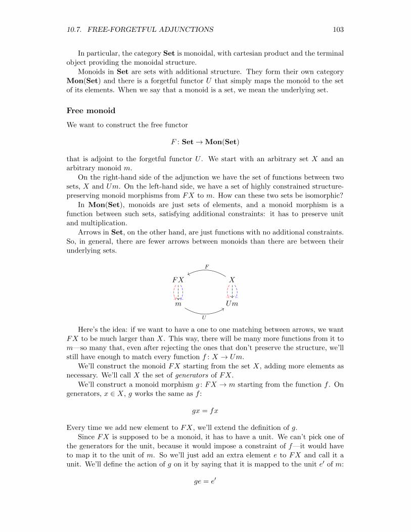
10.7. FREE-FORGETFUL ADJUNCTIONS 103

In particular, the category Set is monoidal, with cartesian product and the terminalobject providing the monoidal structure.

Monoids in Set are sets with additional structure. They form their own categoryMon(Set) and there is a forgetful functor U that simply maps the monoid to the setof its elements. When we say that a monoid is a set, we mean the underlying set.

Free monoid

We want to construct the free functor

F : Set→Mon(Set)

that is adjoint to the forgetful functor U . We start with an arbitrary set X and anarbitrary monoid m.

On the right-hand side of the adjunction we have the set of functions between twosets, X and Um. On the left-hand side, we have a set of highly constrained structure-preserving monoid morphisms from FX to m. How can these two sets be isomorphic?

In Mon(Set), monoids are just sets of elements, and a monoid morphism is afunction between such sets, satisfying additional constraints: it has to preserve unitand multiplication.

Arrows in Set, on the other hand, are just functions with no additional constraints.So, in general, there are fewer arrows between monoids than there are between theirunderlying sets.

FX X

m Um

F

U

Here’s the idea: if we want to have a one to one matching between arrows, we wantFX to be much larger than X. This way, there will be many more functions from it tom—so many that, even after rejecting the ones that don’t preserve the structure, we’llstill have enough to match every function f : X → Um.

We’ll construct the monoid FX starting from the set X, adding more elements asnecessary. We’ll call X the set of generators of FX.

We’ll construct a monoid morphism g : FX → m starting from the function f . Ongenerators, x ∈ X, g works the same as f :

gx = fx

Every time we add new element to FX, we’ll extend the definition of g.

Since FX is supposed to be a monoid, it has to have a unit. We can’t pick one ofthe generators for the unit, because it would impose a constraint of f—it would haveto map it to the unit of m. So we’ll just add an extra element e to FX and call it aunit. We’ll define the action of g on it by saying that it is mapped to the unit e′ of m:

ge = e′


We also have to define monoidal multiplication in FX. Let’s start with a productof two generators a and b. The result of the multiplication cannot be another generatorbecause, again, that would constrain f—products must be mapped to products. So wehave to make all products of generators new elements of FX. Again, the action of g onthose products is fixed:

g(a · b) = ga · gb

Continuing with this construction, any new multiplication produces a new elementof FX, except when it can be reduced to an existing element by applying monoid laws.For instance, the new unit e times a generator a must be equal to a. But we have madesure that e is mapped to the unit of m, so the product ge · ga is automatically equal toga.

Another way of looking at this construction is to think of the set X as an alphabet.The elements of FX are then strings of characters from this alphabet. The generatorsare single-letter strings, “a”, “b”, and so on. The unit is an empty string , “”. Multi-plication is string concatenation, so “a” times “b” is a new string “ab”. Concatenationis automatically associative and unital, with the empty string as the unit.

The intuition behind free functors is that they generate structure “freely,” as in“with no additional constraints.” They do it lazily: instead of performing operations,they just record them.

The free monoid “remembers to do the multiplication” at a later time. It storesthe arguments to multiplication in a string, but doesn’t perform the multiplication.It’s only allowed to simplify its records based on generic monoidal laws. For instance,it doesn’t have to store the command to multiply by the unit. It can also “skip theparentheses” because of associativity.

Exercise 10.7.1. What is the unit and the counit of the free monoid adjunction F a U?

Free monoid in programming

In Haskell, monoids are defined using the following typeclass:

class Monoid m where

mappend :: m -> m -> m

mempty :: m

Here, mappend is the curried form of the mapping from the product (m, m) to m. Themempty element corresponds to the arrow from the terminal object (unit of the monoidalcategory) to m.

A free monoid generated by some type a that is treated as a set of generators, is rep-resented by a list type [a]. An empty list serves as the unit; and monoid multiplicationis implemented as list concatenation, traditionally written in infix form:

(++) :: [a] -> [a] -> [a]

(++) [] ys = ys

(++) (x:xs) ys = x : xs ++ ys

A list is an instance of a Monoid:

instance Monoid [a] where

mempty = []

mappend = (++)

10.8. THE CATEGORY OF ADJUNCTIONS 105

To show that it’s a free monoid, we have to be able to construct a monoid morphismfrom the list of a to an arbitrary monoid m, provided we have an (unconstrained)mapping from a to (the underlying set of) m. We can’t express all of this in Haskell,but we can define the function:

foldMap :: Monoid m => (a -> m) -> ([a] -> m)

foldMap f = foldr mappend mempty . fmap f

This function transforms the elements of the list to monoidal values using f and thenfolds them using mappend, starting with the unit mempty.

It’s easy to see that an empty list is mapped to the monoidal unit. It’s not toohard to see that a concatenation of two lists is mapped to the monoidal product of theresults. So, indeed, foldMap produces a monoid morphism.

Following the intuition of a free monoid being a domain-specific program, foldMapprovides an interpreter for this program. It performs all the multiplications that havebeen postponed. Note that the same program may be interpreted in many ways, de-pending on the choice of the concrete monoid and the function f.

We’ll come back to free monoids as lists in the chapter on algebras.

Exercise 10.7.2. Write a program that takes a list of integers and interprets it in twoways: once using the additive and once using the multiplicative monoid of integers.

10.8 The Category of Adjunctions

We can define composition of adjunctions by taking advantage of the composition offunctors that define them. Two adjunctions, L a R and L′ a R′, are composable if theyshare the category in the middle:

C D ER′

L′

R

L

By composing the functors we get a new adjunction (L′ ◦ L) a (R ◦R′).Indeed, let’s consider the hom-set:

C(L′(Le), c)

Using the L′ a R′ adjunction, we can transpose L′ to the right, where it becomes R′:

D(Le,R′c)

and using L a R we can similarly transpose L:

E(e,R(R′c))

Combining these two isomorphisms, we get the composite adjunction:

C((L′ ◦ L)e, c) ∼= E(e, (R ◦R′)c)

Because functor composition is associative, the composition of adjunctions is alsoassociative. It’s easy to see that a pair of identity functors forms a trivial adjunction


that serves as the identity with respect to composition of adjunctions. Therefore we candefine a category Adj(Cat) in which objects are categories and arrows are adjunctions(by convention, pointing in the direction of the left adjoint).

Adjunctions can be defined purely in terms of functors and natural transformations,that is 1-cells and 2-cells in the 2-category Cat. There is nothing special about Cat,and in fact adjunctions can be defined in any 2-category. Moreover, the category ofadjunctions is itself a 2-category.

10.9 Levels of Abstraction

Category theory is about structuring knowledge. In particular, it can be applied tothe knowledge of category theory itself. Hence we see a lot of mixing of abstractionlevels in category theory. The structures that we see at one level can be grouped intohigher-level structures which exhibit even higher levels of structure, and so on.

In programming we are used to building hierarchies of abstractions. Values aregrouped into types, types into kinds. Functions that operate on values are treateddifferently than functions that operate on types. We often use different syntax toseparate levels of abstractions. Not so in category theory.

A set, categorically speaking, can be described as a discrete category. Elements ofthe set are objects of this category and, other than the obligatory identity morphisms,there are no arrows between them.

The same set can then be seen as an object in the category Set. Arrows in thiscategory are functions between sets.

The category Set, in turn, is an object in the category Cat. Arrows in Cat arefunctors.

Functors between any two categories C and D are objects in the functor category[C,D]. Arrows in this category are natural transformations.

We can define functors between functor categories, product categories, oppositecategories, and so on, ad infinitum.

Completing the circle, hom-sets in every category are sets. We can define mappingsand isomorphisms between them, reaching across disparate categories. Adjunctions arepossible because we can compare hom-sets that live in different categories.

Chapter 11

Dependent Types

We’ve seen types that depend on other types. They are defined using type construc-tors with type parameters, like Maybe or []. Most programming languages have somesupport for generic data types—data types parameterized by other data types.

Categorically, such types are modeled as functors 1.

A natural generalization of this idea is to have types that are parameterized byvalues. For instance, it’s often advantageous to encode the length of a list in its type.A list of length zero would have a different type than a list of length one, and so on.

Types parameterized by values are called dependent types. There are languages likeIdris or Agda that have full support for dependent types. It’s also possible to implementdependent types in Haskell, but support for them is still rather patchy.

The reason for using dependent types in programming is to make programs provablycorrect. In order to do that, the compiler must be able to check the assumptions madeby the programmer.

Haskell, with its strong type system, is able to uncover a lot of bugs at compiletime. For instance, it won’t let you write a <> b (infix notation for mappend), unlessyou provide the Monoid instance for the type of your variables.

However, within Haskell’s type system, there is no way to express or, much lessenforce, the unit and associativity laws for the monoid. For that, the instance of theMonoid type class would have to carry with itself proofs of equality (not actual code):

assoc :: m <> (n <> p) = (m <> n) <> p

lunit :: mempty <> m = m

runit :: m <> mempty = m

Dependent types, and equality types in particular, pave the way towards this goal.

The material in this chapter is more advanced, and not used in the rest of the book,so you may safely skip it on first reading. Also, to avoid confusion between fibers andfunctions, I decided to use capital letters for objects in parts of this chapter.

11.1 Dependent Vectors

We’ll start with the standard example of a counted list, or a vector:

1A type constructor that has no Functor instance can be thought of as a functor from a discretecategory—a category with no arrows other than identities

107

108 CHAPTER 11. DEPENDENT TYPES

data Vec n a where

VNil :: Vec Z a

VCons :: a -> Vec n a -> Vec (S n) a

The compiler will recognize this definition as dependently typed if you include thefollowing language pragmas:

{- # LANGUAGE DataKinds # -}

{- # LANGUAGE GADTs # -}

The first argument to the type constructor is a natural number n. Notice: this is avalue, not a type. The type checker is able to figure this out from the usage of n inthe two data constructors. The first one creates a vector of the type Vec Z a, and thesecond creates a vector of the type Vect (S n) a, where Z and S are defined as theconstructors of natural numbers:

data Nat = Z | S Nat

We can be more explicit about the parameters if we use the pragma:

{- # LANGUAGE KindSignatures # -}

and import the library:

import Data.Kind

We can then specify that n is a Nat, whereas a is a Type:

data Vec (n :: Nat) (a :: Type) where

VNil :: Vec Z a

VCons :: a -> Vec n a -> Vec (S n) a

Using one of these definitions we can, for instance, construct a vector (of integers)of length zero:

emptyV :: Vec Z Int

emptyV = VNil

It has a different type than a vector of length one:

singleV :: Vec (S Z) Int

singleV = VCons 42 VNil

and so on.

We can now define a dependently typed function that returns the first element of avector:

headV :: Vec (S n) a -> a

headV (VCons a _) = a

This function is guaranteed to work exclusively with non-zero-length vectors. Theseare the vectors whose size matches (S n), which cannot be Z. If you try to call thisfunction with emptyV, the compiler will flag the error.

Another example is a function that zips two vectors together. Encoded in its typesignature is the requirement that the two vectors be of the same size n (the result isalso of the size n):

zipV :: Vec n a -> Vec n b -> Vec n (a, b)

zipV (VCons a as) (VCons b bs) = VCons (a, b) (zipV as bs)

11.2. DEPENDENT TYPES CATEGORICALLY 109

zipV VNil VNil = VNil

Exercise 11.1.1. Implement the function tailV that returns the tail of the non-zero-length vector. Try calling it with emptyV.

11.2 Dependent Types Categorically

The easiest way to visualize dependent types is to think of them as families of typesindexed by elements of a set. In the case of counted vectors, the indexing set would bethe set of natural numbers N.

The zeroth type would be the unit type () representing an empty vector. The typecorresponding to (S Z) would be a; then we’d have a pair (a, a), a triple (a, a, a)

and so on, with higher and higher powers of a.If we want to talk about the whole family as one big set, we can take the sum of all

these types. For instance, the sum of all powers of a is the familiar list type, a.k.a, afree monoid:

List(a) =∐n:N

an

Fibrations

Although intuitively easy to visualize, this point of view doesn’t generalize nicely tocategory theory, where we don’t like mixing sets with objects. So we turn this pictureon its head and instead of talking about injecting family members into the sum, weconsider a mapping that goes in the opposite direction.

This, again, we can first visualize using sets. We have one big set E describing thewhole family, and a function p called the projection, or a display map, that goes fromE down to the indexing set B (also called the base).

This function will, in general, map multiple elements to one. We can then talkabout the inverse image of a particular element x ∈ B as the set of elements that getmapped down to it by p. This set is called the fiber and is written p−1x (even though,in general, p is not invertible in the usual sense). Seen as a collection of fibers, E isoften called a fiber bundle or just a bundle.

x

p−1x

B

E

Now forget about sets. A fibration in an arbitrary category is a pair of objects eand b and an arrow p : e→ b.

So this is really just an arrow, but the context is everything. When an arrow is calleda fibration, we use the intuition from sets, and imagine its source e as a collection offibers, with p projecting each fiber down to a single point in the base b.

We can go even further: since (small) categories form a category Cat with functorsas arrows, we can define a fibration of a category, taking another category as its base.


Type families as fibrations

We will therefore model type families as fibrations. For instance, our counted-vectorfamily can be represented as a fibration whose base is the type of natural numbers. Thewhole family is a sum (coproduct) of consecutive powers (products) of a:

List(a) = a0 + a1 + a2 + ... =∐n : N

an

with the zeroth power—the initial object—representing a vector of size zero.

0 1 2 3 4...

The projection p : List(a)→ N is the familiar length function.

Slice categories

In category theory we like to describe things in bulk—defining internal structure ofthings by structure-preserving maps between them. Such is the case with fibrations.

If we fix the base object b and consider all possible source objects in the categoryC, and all possible projections down to b, we get a slice category C/b (also known as anover-category).

An object in the slice category is a pair 〈e, p〉, with p : e → b. An arrow betweentwo objects 〈e, p〉 and 〈e′, p′〉 is an arrow f : e→ e′ that commutes with the projections,that is:

p′ ◦ f = p

Again, the best way to visualize this is to notice that such an arrow maps fibers ofp to fibers of p′. It’s a “fiber-preserving” mapping between bundles.

e e′

b

p

f

p′

Our counted vectors can be seen as objects in the slice category C/N given by pairs〈List(a), length〉.

Coslice categories

There is also a dual notion of a coslice category c/C, also known as an under-category.It’s a category of arrows emanating from a fixed object c. Objects in this categoryare pairs 〈a, i : c → a〉. Morphisms in c/C are arrows that make the relevant trianglescommute.

c

a b

ji

f


In particular, if the category C has a terminal object 1, then the coslice 1/C has, asobjects, global elements of all objects of C.

There is a forgetful functor U : 1/C → C that maps 〈a, i〉 to a. This functor definesa fibration of 1/C. Objects in the fiber over some a are in one-to-one correspondencewith global elements of a.

1

a b

yx

f

Morphisms of 1/C that correspond to an arrow f : a→ b map the set of global elementsof a to the set of global elements of b. Thus this fibration justifies our intuition of typesas sets of values, with values represented by global elements of types.

Pullbacks

We’ve seen a lot of examples of commuting squares. Such a square is a graphicalrepresentation of an equation: two path between opposite corners of a square, each aresult of a composition of two morphisms, are equal.

Like with every equality we may want to replace one or more of its componentswith an unknown, and try to solve the resulting equation. For instance, we may ask thequestion: Is there an object together with two arrows that would complete a commutingsquare? If many such objects exist, is there a universal one? If the missing piece of thepuzzle is the upper left corner of a square (the source), we call it a pullback. If it’s thelower right corner (the target), we call it a pushout.

Let’s start with a particular fibration p : E → B and ask ourselves the question:what happens when we change the base from B to some A that is related to it througha mapping f : A→ B. Can we “pull the fibers back” along f?

Again, let’s think about sets first. Imagine picking a fiber in E over some pointy ∈ B that is in the image of f . We can plant this fiber over all points in A that arein the inverse image f−1y. If multiple points in A are mapped to the same point in B,we just duplicate the corresponding fiber. This way, every point in A will have a fibersticking out of it. The sum of all these fibers will form a new bundle E′.

y BA

EE′

x1 x2

We have thus constructed a new fibration with the base A. Its projection p′ : E′ → Amaps each point in a given fiber to the point over which this fiber was planted. Thereis also an obvious mapping g : E′ → E that maps fibers to their corresponding fibers.

By construction, this new fibration 〈E′, p′〉 satisfies the condition:

p ◦ g = f ◦ p′


which can be represented as a commuting square:

E′ E

A B

p′

g

p

f

In Set, we can explicitly construct E′ as a subset of the cartesian product A × Ewith p′ = π1 and g = π2 (the two cartesian projections). An element of E′ is a pair〈b, e〉, such that:

f(b) = p(e)

This commuting square is the starting point for the categorical generalization. How-ever, even in Set there are many different fibrations over A that make this diagramcommute. We have to pick the universal one. Such a universal construction is called apullback, or a fibered product.

A pullback of p : e → b along f : a → b is an object e′ together with two arrowsp′ : e′ → a and g : e′ → e that makes the above diagram commute, and that satisfies theuniversal condition.

The universal condition says that, for any other candidate object x with two arrowsq′ : x→ e and q : x→ a such that p ◦ q′ = f ◦ q, there is a unique arrow h : x→ e′ thatmakes the two triangles commute:

x

e′ e

a b

h

q′

q

g

p′y

p

f

The angle symbol in the corner of the square is used to mark pullbacks.If we look at the pullback through the prism of sets and fibrations, E is a bundle

over B, and we are constructing a new bundle E′ out of the fibers taken from E. Wherewe plant these fibers over A is determined by (the inverse image of) f . This proceduremakes E′ a bundle over both A and B, the latter with the projection p ◦ g = f ◦ p′.

X in this picture is some other bundle over A with the projection q. It is simulta-neously a bundle over B with the projection f ◦ q = p◦ q′. The unique mapping h mapsthe fibers of X given by q−1 to fibers of E′ given by p′.

All mappings in this picture work on fibers. Some of them rearrange fibers over newbases—that’s what a pullback does. This is analogous to what natural transformationsdo to containers. Others modify individual fibers—the mapping h : G → E′ workslike this. This is analogous to what fmap does to containers. The universal conditionthen tells us that q′ can be factored into a transformation of fibers h, followed by therearrangement of fibers g.

It’s worth noting that picking the singleton set as the pullback target gives usautomatically the definition of the cartesian product:

B × F F

B 1

π1

π2

y!

!


Alternatively, we can think of this picture as planting as many copies of F as thereare elements in B. We’ll use this analogy when we talk about the dependent sum andproduct.

Conversely, a single fiber can be extracted from a fibration by pulling it back to theterminal object. In this case the mapping x : 1→ B picks an element of the base, andthe pullback along it extracts a single fiber F :

F E

1 B

!

g

yp

x

The arrow g injects this fiber back into E. By varying x we can pick different fibers inE.

Exercise 11.2.1. Show that the pullback with the terminal object as the target is theproduct.

Exercise 11.2.2. Show that a pullback can be defined as a limit of the diagram from astick-figure category with three objects:

a→ b← c

Exercise 11.2.3. Show that a pullback in C with the target b is a product in the slicecategory C/b. Hint: Define two projections as morphisms in the slice category. Useuniversality of the pullback to show the universality of the product.

Base-change functor

We used a cartesian closed category as a model for programming. To model dependenttypes, we need to impose an additional condition: We require the category to be locallycartesian closed. This is a category in which all slice categories are cartesian closed.

In particular, such categories have all pullbacks, so it’s always possible to changethe base of any fibration. Base change induces a mapping between slice categories thatis functorial.

Given two slice categories C/b and C/a and an arrow between bases f : b → a thebase-change functor f∗ : C/a → C/b maps a fibration 〈e, p〉 to the fibration f∗〈e, p〉 =〈f∗e, f∗p〉, which is given by the pullback:

f∗e e

b a

yf∗p

g

p

f

Notice that the functor f∗ goes in the opposite direction to the arrow f .

To visualize the base-change functor let’s consider how it works on sets. We havethe intuition that the fibration p decomposes the set E into fibers over each point of A.

But here we have another fibration f that similarly decomposes B. Let’s call thesefibers in B “patches.” For instance, if A is just a two-element set, then the fibrationgiven by f splits B into two patches. The pullback takes a fiber from E and plants it


over the whole patch in B. The resulting set f∗E looks like a patchwork, where eachpatch is planted with clones of a fiber from E.

A

E

B

f∗E

f

Since we have a function from B to A that may map many elements to one, thefibration over B has finer grain than the coarser fibration over A. The simplest, least-effort way to turn the fibration of E over A to a fibration over B, is to spread theexisting fibers over the patches defined by (the inverse of) f . This is the essence of theuniversal construction of the pullback.

You may also think of A as providing an atlas that enumerates all the patches inthe base B.

In particular, if A is a singleton set (the terminal object), then we have only onefiber (the whole of E) and the bundle f∗E is a cartesian product B × E. Such bundleis called a trivial bundle.

A non-trivial bundle is not a product, but it can be locally decomposed into products.Just as B is a sum of patches, so f∗E is a sum of products of these patches and thecorresponding fibers of E.

As we’ll see soon, in a locally cartesian closed category, the base change functor hasboth the left and the right adjoints. The left adjoint is called the dependent sum, andthe right adjoint is called the dependent product (or dependent function).

11.3 Dependent Sum

In type theory, the dependent sum, or the sigma type Σx:BT (x), is defined as a type ofpairs in which the type of the second component depends on the value of the first com-ponent. Our counted vector type can be thought of as a dependent sum. An element ofthis type is a natural number n paired with an n-tuple of values (x_1, x_2, ... x_n)

of the type (a, a, ... a).

The introduction rule for the dependent sum assumes that there is a family oftypes T (x) indexed by elements of the base type B. Then an element of Σx:BT (x) isconstructed from a pair of elements x : B and y : T (x).

Categorically, dependent sum is modeled as the left adjoint of the base-change func-tor.

To see this, let’s first revisit the definition of a pair, which is an element of a product.We’ve noticed before that a product can be written as a pullback from the singletonsent or the terminal object. Here’s the universal construction for the product/pullback

11.3. DEPENDENT SUM 115

(the notation anticipates the target of this construction):

S

B × F F

B 1

φT

φ

qy

π2

π1 !

!

We have also seen that the product can be defined using an adjunction. We canspot this adjunction in our diagram: for every pair of arrows 〈φ, q〉 there is a uniquearrow φT that makes the triangles commute.

Notice that, if we keep q fixed, we get a one-to-one correspondence between thearrows φ and φT . This will be the adjunction we’re interested in.

We can now put our fibrational glasses on and notice that 〈S, q〉 and 〈B×F, π1〉 aretwo fibrations over the same base B. The commuting triangle makes φT a morphismin the slice category C/B, or a fiber-wise mapping. In other words φT is a member ofthe hom-set:

(C/B)

(⟨S

q

⟩,

⟨B × Fπ1

⟩)Since φ is a member of the hom-set C(S, F ), we can rewrite the one-to-one corre-

spondence between φ and φT as an isomorphism of hom-sets:

C(S, F ) ∼= (C/B)

(⟨S

q

⟩,

⟨B × Fπ1

⟩)In fact, it’s an adjunction in which the left functor is the forgetful functor L : C/B → Cthat maps 〈S, q〉 to S, thus forgetting the fibration.

If you squint at this adjunction hard enough, you can see the outlines of the definitionof S as a categorical sum (coproduct).

Firstly, on the left you have a mapping out of S. Think of S as the sum of fibersthat are defined by the fibration 〈S, q〉.

Secondly, recall that the fibration 〈B × F, π1〉 can be though of as producing manycopies of F planted over points in B. Then the right hand side looks like a bunch ofarrows, each mapping a different fiber of S to the same fiber F .

B × F

S

F

B

φT

For comparison, this is the definition of a coproduct of two fibers, with S = F1 +F2:

C(F1 + F2, F ) ∼= (C × C)(〈F1, F2〉,∆F )


Seen in this light, a dependent sum is just a sum of many fibers. In Set it’s a taggedunion. Each individual set is a fiber of S under q.

We can generalize our diagram by replacing the terminal object with an arbitrarybase A. We now have a fibration 〈F, p〉, and we get the pullback square that definesthe base-change functor f∗:

S

f∗F F

B A

φT

φ

q

y

g

f∗p p

f

The universality of the pullback results in the following isomorphism of hom-sets:

(C/A)

(⟨S

f ◦ q

⟩,

⟨F

p

⟩)∼= (C/B)

(⟨S

q

⟩, f∗

⟨F

p

⟩)Here, φ is an element of the left-hand side and φT is the corresponding element of theright-hand side.

We interpret this isomorphism as the adjunction between the base change functorf∗ on the right and the dependent sum functor on the left.

(C/A)

(Σf

⟨S

q

⟩,

⟨F

p

⟩)∼= (C/B)

(⟨S

q

⟩, f∗

⟨F

p

⟩)The dependent sum is thus defined by this formula:

Σf

⟨S

q

⟩=

⟨S

f ◦ q

⟩This says that, if S is fibered over B using q, and there is a mapping f from B to A,then S is automatically fibered over A, the projection being the composition f ◦ q.

We’ve seen before that, in Set, f defines patches within B. Fibers of F are replantedin these patches to form f∗F . Locally—that is within each patch—f∗F looks like acartesian product. Locally, the mapping φT is a product of fiber-wise mappings. So,locally, S is a sum of fibers. Globally, these patches of fibers are summed together intoone whole.

Existential quantification

In the propositions as types interpretation, type families correspond to families of propo-sitions. The dependent sum type Σx:B T (x) corresponds to the proposition: There existsan x for which T (x) is true:

∃x:B T (x)

Indeed, a term of the type Σx:B T (x) is a pair of an element x : B and an elementy : T (x)—which shows that T (x) is inhabited for some x.

11.4. DEPENDENT PRODUCT 117

11.4 Dependent Product

In type theory, the dependent product, or dependent function, or pi-type Πx:BT (x), isdefined as a function whose return type depends on the value of its argument.

It’s called a function, because you can evaluate it. Given a dependent functionf : Πx:BT (x), you may apply it to an argument x : B to get a value f(x) : T (x).

Dependent product in Haskell

A simple example is a function that constructs a vector of a given size and fills it withcopies of a given value:

replicateV :: a -> SNat n -> Vec n a

replicateV _ SZ = VNil

replicateV x (SS n) = VCons x (replicateV x n)

At the time of this writing, Haskell’s support for dependent types is limited, so theimplementation of dependent functions requires the use of singleton types. In this case,the number that is the argument to replicateV is passed as a singleton natural:

data SNat n where

SZ :: SNat Z

SS :: SNat n -> SNat (S n)

(Note that replicateV is a function of two arguments, so it can be either considered adependent function of a pair, or a regular function returning a dependent function.)

Dependent product of sets

Before we describe the categorical model of dependent functions, it’s instructive toconsider how they work on sets. A dependent function selects one element from eachset T (x).

You may visualize this selection as a large tuple—or an element of the cartesianproduct that you get by multiplying together all the sets in the family. This is themeaning of the product notation, Πx:BT (x). For instance, in the trivial case of B atwo-element set {1, 2}, a dependent function is just a cartesian product T (1)× T (2).

In our example, replicateV picks a particular counted vector for each value of n.Counted vectors are equivalent to tuples so, for n equal zero, replicateV returns anempty tuple (); for n equals one it returns a single value x; for n equals two, it returnsa homogenous pair (x, x); etc.

The function replicateV, evaluated at some x :: a, is equivalent to an infinitetuple of tuples:

((), x, (x, x), (x, x, x), ...)

which is a specific element of the more general type:

((), a, (a, a), (a, a, a), ...)

Dependent product categorically

In order to build a categorical model of dependent functions, we need to change ourperspective from a family of types to a fibration. We start with a bundle E/B fiberedby the projection p : E → B. A dependent function is called a section of this bundle.


If you visualize the bundle as a bunch of fibers sticking out from the base B, asection is like a haircut: it cuts through each fiber to produce a corresponding value.In physics, such sections are called fields—with spacetime as the base.

Just like we talked about a function object representing a set of functions, we cantalk about an object S(E) that represents a set of sections of a given bundle E.

Just like we defined function application as a mapping out of the product:

εB,C : CB ×B → C

we can define the dependent function application as a mapping:

ε : S(E)×B → E

We can visualize it as picking a section s in S and an element x of the base B andproducing a value in the bundle E. (In physics, this would correspond to measuring afield at a particular point in spacetime.)

But this time we have to insist that this value be in the correct fiber. If we projectthe result of applying ε to (s, x), we should get the same x.

ε(s, x)

s

x

p−1x

B

E

In other words, this diagram should commute:

S(E)×B E

B

ε

π2 p

This makes ε a morphism in the slice category C/B.And just like the exponential object was universal, so is the object of sections.

The universality condition has the same form: for any other object G with an arrowφ : G×B → E there is a unique arrow φT : G→ S(E) that makes the following diagramcommute:

G×B

S(E)×B E

φT×B φ

ε

The difference is that now both ε and φ are now morphisms in the slice category C/B.The one-to-one correspondence between φ and φT forms an adjunction:

(C/B)

(⟨G×Bπ2

⟩,

⟨E

p

⟩)∼= C (G,S(E))

which we can use as the definition of the object of sections S(E).

11.4. DEPENDENT PRODUCT 119

Recall that we can interpret the product G×B as planting copies of G as identicalfibers over each element of B.

In Set, a single morphism on the left-hand side is equivalent to a family of functions,one per fiber. Any given x ∈ G produces a horizontal slice of G × B. Our family offunctions maps this slice to the corresponding fibers of E thus creating a section of E.

B

G

G×B

B

E

The adjunction tells us that this family of mappings uniquely determines a functionfrom G to S(E). Every x ∈ G is thus mapped to a different element s of S(E). Thereforeelements of S(E) are in one-to-one correspondence with sections of E .

These are all set-theoretical intuitions. We can generalize them by first noticingthat the right hand side of the adjunction can be easily expressed as a hom-set in theslice category C/1 over the terminal object.

Indeed, there is one-to-one correspondence between objects X in C and objects 〈X, !〉in C/1. Arrows in C/1 are arrows of C with no additional constraints. We thereforehave:

(C/B)

(⟨G×Bπ2

⟩,

⟨E

p

⟩)∼= (C/1)

(⟨G

!

⟩,

⟨S(E)

!

⟩)

The next step is to “blur the focus” by replacing the terminal object with a moregeneral base A.

The right-hand side becomes a hom-set in the slice category C/A and G gets fibratedby some q : G→ A.

We can then replace the product G × B with a more general pullback of q alongsome f : B → A.

G×B G

B 1

yπ2

π1

!

!

f∗G G

B A

yf∗q

g

q

f

The result is that, instead of a bunch of G fibers over B, we get a pullback f∗Gthat is populated by groups of fibers from the fibration q : G→ A. This way, A servesas an atlas that enumerates all the uniform patches.

Imagine, for instance, that A is a two-element set. The fibration q will split G intotwo fibers. These will be our generic fibers. These fibers are now replanted over thetwo patches in B to form f∗G. The replanting is guided by f−1.


A

G

B

f∗G

fB

E

The adjunction that defines the dependent function type is therefore:

(C/B)

(f∗⟨G

q

⟩,

⟨E

p

⟩)∼= (C/A)

(⟨G

q

⟩,Πf

⟨E

p

⟩)where ΠfE is a suitable rearrangement of the object of sections S(E). The adjunctionis a mapping between morphisms in their respective slice categories:

f∗G E

B

φ

f∗q p

G ΠfE

A

φT

qΠf p

To gain some intuition into this adjunction, let’s consider how it works on sets.The right hand side operates in a coarsely grained fibration over the atlas A. It’s a

family of functions, one function per patch. For every patch we get a function from the“thick fiber” of G (drawn in blue below) to the “thick fiber” of ΠfE.

The left hand side operates in a more finely grained fibration over B. These fibersare grouped into small bundles over patches. Once we pick a patch (drawn in redbelow), we get a family of functions from that patch to the corresponding patch inE—a section of a small bundle in E. So, patch-by-patch, we get small sections of E.

The adjunction tells us that the elements of the “thick fiber” of ΠfE correspond tosmall sections of E over the same patch.

E

B

G

Aq

f

p

The following exercises shed some light on the role played by f . It can be seen aslocalizing the sections of E by restricting them to “neighborhoods” defined by f−1.

Exercise 11.4.1. Consider what happens when A is a two-element set {0, 1} and fmaps the whole of B to one element, say 1. How would you define the function on theright-hand side of the adjunction? What should it do to the fiber over 0?

11.5. EQUALITY 121

Exercise 11.4.2. Let’s pick G to be a singleton set 1, and let x : 1→ A be a fibrationthat selects an element in A. Using the adjunction, show that:

• f∗1 has two types of fibers: singletons over the elements of f−1(x) and empty setsotherwise.

• A mapping φ : f∗1 → E is equivalent to a selection of elements, one from eachfiber of E over the elements of f−1(x). In other words, it’s a partial section of Eover the subset f−1(x) of B.

• A fiber of ΠfE over a given x is such a partial section.

• What happens when A is also a singleton set?

Universal quantification

The logical interpretation of the dependent product Πx:B T (x) is a universally quaniti-fied proposition. An element of Πx:B T (x) is a section—the proof that it’s possible toselect an element from each member of the family T (x). It means that none of them isempty. In other words, it’s a proof of the proposition:

∀x:B T (x)

11.5 Equality

Our first experience in mathematics involves equality. We learn that

1 + 1 = 2

and we don’t think much of it afterwards.But what does it mean that 1 + 1 is equal to 2? Two is a number, but one plus one

is an expression, so they are not the same thing. There is some mental processing thatwe have to perform before we pronounce these two things equal.

Contrast this with the statement 0 = 0, in which both sides of equality are the samething.

It makes sense that, if we are to define equality, we’ll have to at least make surethat everything is equal to itself. We call this property reflexivity.

Recall our definition of natural numbers:

data Nat where

Z :: Nat

S :: Nat -> Nat

This is how we can define equality for natural numbers:

equal :: Nat -> Nat -> Bool

equal Z Z = True

equal (S m) (S n) = equal m n

equal _ _ = False

We are recursively stripping S’s in each number until one of them reaches Z. If theother reaches Z at the same time, we pronounce the numbers we started with to beequal, otherwise they are not.


Equational reasoning

Notice that, when defining equality in Haskell, we were already using the equal sign.For instance, the equal sign in:

equal Z Z = True

tells us that wherever we see the expression equal Z Z we can replace it with True andvice versa.

This is the principle of substituting equals for equals, which is the basis for equationalreasoning in Haskell. We can’t encode proofs of equality directly in Haskell, but we canuse equational reasoning to reason about Haskell programs. This is one of the mainadvantages of pure functional programming. You can’t perform such substitutions inimperative languages, because of side effects.

If we want to prove that 1 + 1 is 2, we have to first define addition. The definitioncan either be recursive in the first or in the second argument. This one recurses in thesecond argument:

add :: Nat -> Nat -> Nat

add n Z = n

add n (S m) = S (add n m)

We encode 1 + 1 as:

add (S Z) (S Z)

We can now use the definition of add to simplify this expression. We try to matchthe first clause, and we fail, because S Z is not the same as Z. But the second clausematches. In it, n is an arbitrary number, so we can substitute S Z for it, and get:

add (S Z) (S Z) = S (add (S Z) Z)

In this expression we can perform another substitution of equals using the first clauseof the definition of add (again, with n replaced by S Z):

add (S Z) Z = (S Z)

We arrive at:

add (S Z) (S Z) = S (S Z)

We can clearly see that the right-hand side is the encoding of 2. But we haven’t shownthat our definition of equality is reflexive so, in principle, we don’t know if:

eq (S (S Z)) (S (S Z))

yields True. We have to use step-by-step equational reasoning again:

equal (S (S Z) (S (S Z)) =

{- second clause of the definition of equal -}

equal (S Z) (S Z) =

{- second clause of the definition of equal -}

equal Z Z =

{- first clause of the definition of equal -}

True

We can use this kind of reasoning to prove statements about concrete numbers, butwe run into problems when reasoning about generic numbers—for instance, showingthat something is true for all n. Using our definition of addition, we can easily show

11.5. EQUALITY 123

that add n Z is the same as n. But we can’t prove that add Z n is the same as n. Thelatter proof requires the use of induction.

We end up distinguishing between two kinds of equality. One is proven using sub-stitutions, or rewriting rules, and is called definitional equality. You can think of itas macro expansion or inline expansion in programming languages. It also involves β-reductions: performing function application by replacing formal parameters by actualarguments, as in:

(\x -> x + x) 2 =

{- beta reduction -}

2 + 2

The second more interesting kind of equality is called propositional equality and itmay require actual proofs.

Equality vs isomorphism

We said that category theorists prefer isomorphism over equality—at least when itcomes to objects. It is true that, within the confines of a category, there is no wayto differentiate between isomorphic objects. In general, though, equality is strongerthan isomorphism. This is a problem, because it’s very convenient to be able to substi-tute equals for equals, but it’s not always clear that one can substitute isomorphic forisomorphic.

Mathematicians have been struggling with this problem, mostly trying to modify thedefinition of isomorphism—but a real breakthrough came when they decided to simul-taneously weaken the definition of equality. This led to the development of homotopytype theory, or HoTT for short.

Roughly speaking, in type theory, specifically in Martin-Lof theory of dependenttypes, equality is represented as a type, and in order to prove equality one has toconstruct an element of that type—in the spirit of the Curry-Howard interpretation.

Furthermore, in HoTT, the proofs themselves can be compared for equality, and soon ad infinitum. You can picture this by considering proofs of equality not as pointsbut as some abstract paths that can be morphed into each other; hence the languageof homotopies.

In this setting, instead of isomorphism, which involves strict equalities of arrows:

f ◦ g = id

g ◦ f = id

one defines an equivalence, in which these equalities are treated as types.

The main idea of HoTT is that one can impose the univalence axiom which, roughlyspeaking, states that equalities are equivalent to equivalences, or symbolically:

(A = B) ∼= (A ∼= B)

Notice that this is an axiom, not a theorem. We can either take it or leave it and thetheory is still valid (at least we think so).


Equality types

Suppose that you want to compare two terms for equality. The first requirement isthat both terms be of the same type. You can’t compare apples with oranges. Don’tget confused by some programming languages allowing comparisons of unlike terms: inevery such case there is an implicit conversion involved, and the final equality is alwaysbetween same-type values.

For every pair of values there is, in principle, a separate type of proofs of equality.There is a type for 0 = 0, there is a type for 1 = 1, and there is a type for 1 = 0; thelatter hopefully uninhabited.

Equality type, a.k.a., identity type, is therefore a dependent type: it depends onthe two values that we are comparing. It’s usually written as IdA, where A is the typeof both values, or using an infix notation as x =A y (equal sign with the subscript A).

For instance, the type of equality of two zeros is written as IdN(0, 0) or:

0 =N 0

Notice: this is not a statement or a term. It’s a type, like Int or Bool. You can definea value of this type if you have an introduction rule for it.

Introduction rule

The introduction rule for the equality type is the dependent function:

reflA : Πx:AIdA(x, x)

which can be interpreted in the spirit of propositions as types as the proof of thestatement:

∀x:A x = x

This is the familiar reflexivity: it shows that, for all x of type A, x is equal to itself.You can apply this function to some concrete value x of type A, and it will produce anew value of type IdA(x, x).

We can now prove that 0 = 0. We can execute reflN(0) to get a value of the type0 =N 0. This value is the proof that the type is inhabited, and therefore corresponds toa true proposition.

This is the only introduction rule for equality, so you might think that all proofs ofequality boil down to “they are equal because they are the same.” Surprisingly, this isnot the case.

β-reduction and η-conversion

In type theory we have this interplay of introduction and elimination rules that essen-tially makes them the inverse of each other.

Consider the definition of a product. We introduce it by providing two values, x : Aand y : B and we get a value p : A × B. We can then eliminate it by extracting twovalues using two projections. But how do we know if these are the same values that weused to construct it? This is something that we have to postulate (in the categoricalmodel this follows from the universal construction). We call it the computation rule orthe β-reduction rule.

11.5. EQUALITY 125

Conversely, if we are given a value p : A × B, we can extract the two componentsusing projections, and then use the introduction rule to recompose it. But how do weknow that we’ll get the same p? This too has to be postulated. This is sometimes calledthe uniqueness condition, or the η-conversion rule.

The equality type also has the elimination rule, which we’ll discuss shortly, but wedon’t impose the uniqueness condition. It means that it’s possible that there are someequality proofs that were not obtained using refl .

This is exactly the weakening of the notion of equality that makes HoTT interestingto mathematicians.

Induction principle for natural numbers

Before formulating the elimination rule for equality, it’s instructive to first discuss asimpler elimination rule for natural numbers. We’ve already seen such rule describingprimitive recursion. It allowed us to define recursive functions by specifying a valueinit and a function step.

Using dependent types, we can generalize this rule to define the dependent elimina-tion rule that is equivalent to the principle of mathematical induction.

The principle of induction can be described as a device to prove, in one fell swoop,whole families of propositions indexed by natural numbers. For instance, the statementthat add Z n is equal to n is really an infinite number of propositions, one per eachvalue of n.

We could, in principle, write a program that would meticulously verify this state-ment for a very large number of cases, but we’d never be sure if it holds in general.There are some conjectures about natural numbers that have been tested this way usingcomputers but, obviously, they can never exhaust an infinite set of cases.

Roughly speaking, we can divide all mathematical theorems into two groups: theones that can be easily formulated and the ones whose formulation is complex. Theycan be further subdivided into the ones whose proofs are simple, and the ones that arehard or impossible to prove. For instance, the famous Fermat’s Last Theorem was ex-tremely easy to formulate, but its proof required some massively complex mathematicalmachinery.

Here, we are interested in theorems about natural numbers that are both easy toformulate and easy to prove. We’ll assume that we know how to generate a family ofpropositions or, equivalently, a dependent type T (n), where n is a natural number.

We’ll also assume that we have a value:

init : T (Z)

or, equivalently, the proof of the zeroth proposition; and a dependent function:

step : Πn:N (T (n)→ T (Sn))

This function is interpreted as generating a proof of the (n+ 1)st proposition from theproof of the nth proposition.

The dependent elimination rule for natural numbers tells us that, given such initand step, there exists a dependent function:

f : Πn:N T (n)


This function is interpreted as providing the proof that T (n) is true for all n.Moreover, this function, when applied to zero reproduces init :

f(Z) = init

and, when applied to the successor of n, is consistent with taking a step:

f(Sn) = (step(n))(f(n))

(Here, step(n) produces a function, which is then applied to the value f(n).) These arethe two computation rules for natural numbers.

Notice that the induction principle is not a theorem about natural numbers. It’spart of the definition of the type of natural numbers.

Not all dependent mappings out of natural numbers can be decomposed into initand step, just as not all theorems about natural numbers can be proven inductively.There is no η-conversion rule for natural numbers.

Equality elimination rule

The elimination rule for equality type is somewhat analogous to the induction principlefor natural numbers. There we used init to ground ourselves at the start of the journey,and step to make progress. The elimination rule for equality requires a more powerfulgrounding, but it doesn’t have a step. There really is no good analogy for how it works,other than through a leap of faith.

The idea is that we want to construct a mapping out of the equality type. But sinceequality type is itself a two-parameter family of types, the mapping out should be adependent function. The target of this function is another family of types:

T (x, y, p)

that depends on the pair of values that are being compared x, y : A and the proof ofequality p : Id(x, y).

The function we are trying to construct is:

f : Πx,y:AΠp:Id(x,y) T (x, y, p)

It’s convenient to think of it as generating a proof that for all points x and y, andfor every proof that the two are equal, the proposition T (x, y, p) is true. Notice that,potentially, we have a different proposition for every proof that the two points are equal.

The least that we can demand from T (x, y, p) is that it should be true when x andy are literally the same, and the equality proof is the obvious refl . This requirementcan be expressed as a dependent function:

t : Πx:A T (x, x, refl(x))

Notice that we are not even considering proofs of x = x, other than those given byreflexivity. Do such proofs exist? We don’t know and we don’t care.

So this is our grounding, the starting point of a journey that should lead us todefining our f for all pairs of points and all proofs of equality. The intuition is that weare defining f as a function on a plane (x, y), with a third dimension given by p. To do

11.5. EQUALITY 127

that, we’re given something that’s defined on the diagonal (x, x), with p restricted torefl .

refl

p : Id(x, y)

x

y

You would think that we need something more, some kind of a step that wouldmove us from one point to another. But, unlike with natural numbers, there is no nextpoint or next equality proof to jump to. All we have at our disposal is the function tand nothing else.

Therefore we postulate that, given a type family T (x, y, p) and a function:

t : Πx:A T (x, x, refl(x))

there exists a function:f : Πx,y:AΠp:Id(x,y) T (x, y, p)

such that (computation rule):

f(x, x, refl(x)) = t(x)

Notice that the equality in the computation rule is definitional equality, not a type.Equality elimination tells us that it’s alway possible to extend the function t, which

is defined on the diagonal, to the whole 3-d space.This is a very strong postulate. One way to understand it is to argue that, within

the framework of type theory—which is formulated using the language of introductionand elimination rules, and the rules for manipulating those—it’s impossible to define atype family T (x, y, p) that would not satisfy the equality elimination rule.

The closest analogy that we’ve seen so far is the result of parametricity, which statesthat, in Haskell, all polymorphic functions between endofunctors are automaticallynatural transformations. Another example, this time from calculus, is that any analyticfunction defined on the real axis has a unique extension to the whole complex plane.

The use of dependent types blurs the boundary between programming and math-ematics. There is a whole spectrum of languages, with Haskell barely dipping its toesin dependent types while still firmly established in commercial usage; all the way totheorem provers, which are helping mathematicians formalize mathematical proofs.

Chapter 12

Algebras

The essence of algebra is the formal manipulation of expressions. But what is anexpression, and how do we manipulate it?

The first things to observe about algebraic expressions like 2(x+ y) or ax2 + bx+ cis that there are infinitely many of them. There is a finite number of rules for makingthem, but these rules can be used in infinitely many combinations. This suggests thatthe rules are used recursively.

In programming, expressions are virtually synonymous to (parsing) trees. Considerthis simple example of an arithmetic expression:

data Expr = Val Int

| Plus Expr Expr

It’s a recipe for building trees. We start with little trees using the Val constructor. Wethen plant these seedlings into nodes, and so on.

e2 = Val 2

e3 = Val 3

e5 = Plus e2 e3

e7 = Plus e5 e2

Such recursive definitions work perfectly well in a programming language. Theproblem is that every new recursive data structure would require its own library offunctions that operate on it.

From type-theory point of view, we’ve been able to define recursive types, such asnatural numbers or lists, by providing, in each case, specific introduction and eliminationrules. What we need is something more general, a procedure for generating arbitraryrecursive types from simpler pluggable components.

There are two orthogonal concerns when it comes to recursive data structures. Oneis the machinery of recursion. The other is the pluggable components to be used byrecursion.

We know how to work recursion: We assume that we know how to construct smalltrees. Then we use the recursive step to plant those trees into nodes to make biggertrees.

Category theory tells us how to formalize this imprecise description.

129

130 CHAPTER 12. ALGEBRAS

12.1 Algebras from Endofunctors

The idea of planting smaller trees into nodes requires that we formalize what it meansto have a data structure with holes—a “container for stuff.” This is exactly whatfunctors are for. Because we want to use these functors recursively, they have to beendo-functors.

For instance, the endofunctor from our earlier example would be defined by thefollowing data structure, where x marks the spots:

data ExprF x = ValF Int

| PlusF x x

Information about all possible shapes of expressions is abstracted into a single functor.

The other important piece of information is the recipe for evaluating expressions.This, too, can be encoded using the same endofunctor.

Thinking recursively, let’s assume that we know how to evaluate all subtrees of alarger expression. Then the remaining step is to plug these results into the top levelnode and evaluate it.

For instance, suppose that the x’s in the functor were replaced by integers—theresults of evaluation of the subtrees. It’s pretty obvious what we should do in thelast step. If the top of the tree is a leaf ValF (which means there were no subtrees toevaluate) we’ll just return the integer stored in it. If it’s a PlusF node, we’ll add thetwo integers in it. This recipe can be encoded as:

eval :: ExprF Int -> Int

eval (ValF n) = n

eval (PlusF m n) = m + n

We have made some seemingly obvious assumptions based on our experience. Forinstance, since the node was called PlusF we assumed that we should add the twonumbers. But multiplication or subtraction would work equally well.

Since the leaf ValF contained an integer, we assumed that the expression shouldevaluate to an integer. But there is an equally plausible evaluator that pretty-printsthe expression by converting it to a string, and which uses concatenation instead ofaddition:

pretty :: ExprF String -> String

pretty (ValF n) = show n

pretty (PlusF s t) = s ++ " + " ++ t

In fact there are infinitely many evaluators, some sensible, others less so, but weshouldn’t be judgmental. Any choice of the target type and any choice of the evaluatorshould be equally valid. This leads to the following definition:

An algebra for an endofunctor F is a pair (c, α). The object c is called the carrierof the algebra, and the evaluator α : Fc→ c is called the structure map.

In Haskell, given the functor f we define:

type Algebra f c = f c -> c

Notice that the evaluator is not a polymorphic function. It’s a specific choice of afunction for a specific type c. There may be many choices of the carrier types and therebe many different evaluators for a given type. They all define separate algebras.

We have previously defined two algebras for ExprF. This one has Int as a carrier:

12.2. CATEGORY OF ALGEBRAS 131

eval :: Algebra ExprF Int

eval (ValF n) = n

eval (PlusF m n) = m + n

and this one has String as a carrier:

pretty :: Algebra ExprF String

pretty (ValF n) = show n

pretty (PlusF s t) = s ++ " + " ++ t

12.2 Category of Algebras

Algebras for a given endofunctor F form a category. An arrow in that category is analgebra morphism, which is a structure-preserving arrow between their carrier objects.

Preserving structure in this case means that the arrow must commute with thetwo structure maps. This is where functoriality comes into play. To switch from onestructure map to another, we have to be able to lift an arrow that goes between theircarriers.

Given an endofunctor F , an algebra morphism between two algebras (a, α) and (b, β)is an arrow f : a→ b that makes this diagram commute:

Fa Fb

a b

Ff

α β

f

In other words, the following equation must hold:

f ◦ α = β ◦ Ff

The composition of two algebra morphisms is again an algebra morphism, which canbe seen by pasting together two such diagrams. The identity arrow is also an algebramorphism, because

ida ◦ α = α ◦ F (ida)

(a functor maps identity to identity).

The commuting condition in the definition of an algebra morphism is very restrictive.Consider for instance a function that maps an integer to a string. In Haskell there is ashow function (actually, a method of the Show class) that does it. It is not an algebramorphism from eval to pretty.

Exercise 12.2.1. Show that show is not an algebra morphism. Hint: Consider whathappens to the PlusF node.

Initial algebra

The initial object in the category of algebras is called the initial algebra and, as we’llsee, it plays a very important role.

By definition, the initial algebra (i, ι) has a unique algebra morphism f from it toany other algebra (a, α). Diagrammatically:


Fi Fa

i a

Ff

ι α

f

This unique morphism is called a catamorphism for the algebra (a, α).

Exercise 12.2.2. Let’s define two algebras for the following functor:

data FloatF x = Num Float | Op x x

The first algebra:

addAlg :: Algebra FloatF Float

addAlg (Num x) = log x

addAlg (Op x y) = x + y

The second algebra:

mulAlg :: Algebra FloatF Float

mulAlg (Num x) = x

mulAlg (Op x y) = x * y

Make a convincing argument that log (logarithm) is an algebra morphism between thesetwo. (Float is a built-in floating-point number type.)

12.3 Lambek’s Lemma and Fixed Points

Lambek’s lemma says that the structure map ι of the initial algebra is an isomorphism.

The reason for it is the self-similarity of algebras. You can lift any algebra (a, α) us-ing F , and the result (Fa, Fα) is also an algebra with the structure map Fα : F (Fa)→Fa.

In particular, if you lift the initial algebra (i, ι), you get an algebra with the carrierFi and the structure map Fι : F (Fi)→ Fi. It follows then that there must be a uniquealgebra morphism from the initial algebra to it:

Fi F (Fi)

i F i

Fh

ι F ι

h

This h is the inverse of ι. To see that, let’s consider the composition ι ◦ h. It is thearrow at the bottom of the following diagram

Fi F (Fi) Fi

i F i i

Fh

ι F ι

F ι

ι

h ι

This is a pasting of the original diagram with a trivially commuting diagram. Thereforethe whole rectangle commutes. We can interpret this as ι◦h being an algebra morphism

12.3. LAMBEK’S LEMMA AND FIXED POINTS 133

from (i, ι) to itself. But there already is such an algebra morphism—the identity. So,by uniqueness of the mapping out from the initial algebra, these two must be equal:

ι ◦ h = idi

Knowing that, we can now go back to the previous diagram, which states that:

h ◦ ι = Fι ◦ Fh

Since F is a functor, it maps composition to composition and identity to identity.Therefore the right hand side is equal to:

F (ι ◦ h) = F (idi) = idFi

We have thus shown that h is the inverse of ι, which means that ι is an isomorphism.In other words:

Fi ∼= i

We interpret this identity as stating that i is a fixed point of F (up to isomorphism).The action of F on i “doesn’t change it.”

There may be many fixed points, but this one is the least fixed point because thereis an algebra morphism from it to any other fixed point. The least fixed point of anendofunctor F is denoted µF , so we have:

i = µF

Fixed point in Haskell

Let’s consider how the definition of the fixed point works with our original example:

data ExprF x = ValF Int | PlusF x x

Its fixed point is a data structure defined by the property that ExprF acting on itreproduces it. If we call this data structure Expr, the fixed point equation becomes (inpseudo-Haskell):

Expr = ExprF Expr

Expanding ExprF we get:

Expr = ValF Int | PlusF Expr Expr

Compare this with the recursive definition (actual Haskell):

data Expr = Val Int | Plus Expr Expr

We get a recursive data structure as a solution to the fixed-point equation.In Haskell, we can define a fixed point data structure for any functor (or even just

a type constructor). As we’ll see later, this doesn’t always give us the carrier of theinitial algebra. It only works for those functors that have the “leaf” component.

Let’s call Fix f the fixed point of a functor f. Symbolically, the fixed-point equationcan be written as:

f(Fixf) ∼= Fixf

or, in code,


data Fix f where

In :: f (Fix f) -> Fix f

The data constructor In is exactly the structure map of the initial algebra whose carrieris Fix f. Its inverse is:

out :: Fix f -> f (Fix f)

out (In x) = x

The Haskell standard library contains a more idiomatic definition:

newtype Fix f = Fix { unFix :: f (Fix f) }

To create terms of the type Fix f we often use “smart constructors.” For instance,with the ExprF functor, we would define:

val :: Int -> Fix ExprF

val n = In (ValF n)

plus :: Fix ExprF -> Fix ExprF -> Fix ExprF

plus e1 e2 = In (PlusF e1 e2)

and use it to generate expression trees like this one:

e9 :: Fix ExprF

e9 = plus (plus (val 2) (val 3)) (val 4)

12.4 Catamorphisms

Our goal, as programmers, is to be able to perform a computation over a recursive datastructure—to “fold” it. We now have all the ingredients.

The data structure is defined as a fixed point of a functor. An algebra for thisfunctor defines the operation we want to perform. We’ve seen the fixed point and thealgebra combined in the following diagram:

Fi Fa

i a

Ff

ι α

f

that defines the catamorphism f for the algebra (a, α).The final piece of information is the Lambek’s lemma, which tells us that ι could

be inverted because it’s an isomorphism. It means that we can read this diagram as:

f = α ◦ Ff ◦ ι−1

and interpret it as a recursive definition of f .Let’s redraw this diagram using Haskell notation. The catamorphism depends on

the algebra so, for the algebra with the carrier a and the evaluator alg, we’ll have thecatamorphism cata alg.

f (Fix f) f a

Fix f a

fmap (cata alg)

algoutcata alg

12.4. CATAMORPHISMS 135

By simply following the arrows, we get this recursive definition:

cata :: Functor f => Algebra f a -> Fix f -> a

cata alg = alg . fmap (cata alg) . out

Here’s what’s happening: cata alg is applied to some Fix f. Every Fix f isobtained by applying In to a functorful of Fix f. The function out “strips” this dataconstructor.

We can evaluate the functorful of Fix f by fmap’ing cata alg over it. This is arecursive application. The idea is that the trees inside the functor are smaller thanthe original tree, so the recursion eventually terminates. It terminates when it hits theleaves.

After this step, we are left with a functorful of values, and we apply the evaluatoralg to it, to get the final result.

The power of this approach is that all the recursion is encapsulated in one data typeand one library function: We have the definition of Fix and the catamorphism. Theclient of the library has only to provide the non-recursive pieces: the functor and thealgebra. These are much easier to deal with.

Examples

We can immediately apply this construction to our earlier examples. You can checkthat:

cata eval e9

evaluates to 9 and

cata pretty e9

evaluates to the string "2 + 3 + 4".

Sometimes we want to display the tree on multiple lines with indentation. Thisrequires passing a depth counter to recursive calls. There is a clever trick that uses afunction type as a carrier:

pretty' :: Algebra ExprF (Int -> String)

pretty' (ValF n) i = indent i ++ show n

pretty' (PlusF f g) i = f (i + 1) ++ "\n" ++

indent i ++ "+" ++ "\n" ++

g (i + 1)

The auxiliary function indent replicates the space character:

indent n = replicate (n * 2) ' '

The result of:

cata pretty' e9 0

when printed, looks like this:

2

+

3

+

4


Let’s try defining algebras for other familiar functors. The fixed point of the Maybe

functor:

data Maybe x = Nothing | Just x

after some renaming, is equivalent to the type of natural numbers

data Nat = Z | S Nat

An algebra for this functor consists of a choice of the carrier a and an evaluator:

alg :: Maybe a -> a

The mapping out of Maybe is determined by two things: the value corresponding toNothing and a function a->a corresponding to Just. In our discussion of the type ofnatural numbers we called these init and step. We can now see that the eliminationrule for Nat is the catamorphism for this algebra.

Lists as initial algebras

The list type that we’ve seen previously is equivalent to a fixed point of the followingfunctor:

data ListF a x = NilF | ConsF a x

An algebra for this functor is a mapping out

alg :: ListF a c -> c

alg NifF = init

alg (ConsF a c) = step (a, c)

which is determined by the value init and the function step:

init :: c

step :: (a, c) -> c

A catamorphism for such an algebra is the list recursor:

recList :: c -> ((a, c) -> c) -> (List a -> c)

where (List a) is can be identified with the fixed point Fix (ListF a).

We’ve seen before a recursive function that reverses a list. It was implemented byappending elements to the end of a list, which is very inefficient. It’s easy to rewritethis function using a catamorphism, but the problem remains.

Prepending elements, on the other hand, is cheap. A better algorithm would traversethe list, accumulating elements in a first-in-first-out queue, and then pop them one-by-one and prepend them to a new list.

The queue regimen can be implemented by using composition of closures: eachclosure is a function that remembers its environment. Here’s the algebra whose carrieris a function type:

revAlg :: Algebra (ListF a) ([a]->[a])

revAlg NilF = id

revAlg (ConsF a f) = \as -> f (a : as)

At each step, this algebra creates a function that will apply the previous function f tothe result of prepending the current element a to its argument. It’s this element that’sremembered by the closure. The catamorphism for this algebra accumulates a queue

12.5. INITIAL ALGEBRA FROM UNIVERSALITY 137

of such closures. To reverse a list, we apply the result of the catamorphism for thisalgebra to an empty list:

reverse :: Fix (ListF a) -> [a]

reverse as = (cata revAlg as) []

This trick is at the core of the fold-left funcion, foldl. Care should be taken whenusing it, because of the danger of stack overflow.

Lists are so common that their eliminators (called “folds”) are included in the stan-dard library. But there are infinitely many possible recursive data structures, eachgenerated by its own functor, and we can use the same catamorphism on all of them.

It’s worth mentioning that the list construction works in any monoidal categorywith coproducts. We can replace the list functor with a more general:

Fx = I + a⊗ x

where I is the unit object and ⊗ is the tensor product. The solution to the fixed pointequation:

La ∼= I + a⊗ Lacan be formally written as a series:

La = I + a+ a⊗ a+ a⊗ a⊗ a+ ...

We interpret this as a definition of a list, which can be empty I, a singleton a, atwo-element list a⊗ a and so on.

Incidentally, if you squint hard enough, this solution can be obtained by followinga sequence of formal transformations:

La ∼= I + a⊗ LaLa − a⊗ La ∼= I

(I − a)⊗ La ∼= I

La ∼= I/(I − a)

La ∼= I + a+ a⊗ a+ a⊗ a⊗ a+ ...

where the last step uses the formula for the sum of geometric series. Admittedly, theintermediate steps make no sense, since there is no subtraction or division defined onobjects, yet the final result make sense, and it may be made rigorous by considering acolimit of a chain of objects.

12.5 Initial Algebra from Universality

Another way of looking at the initial algebra, at least in Set, is to view it as a collectionof catamorphisms that, as a whole, hint at the existence of an underlying object. Insteadof seeing µF as a set of trees, we can look at it as a set of functions from algebras totheir carriers.

In a way, this is just another manifestation of the Yoneda lemma: every data struc-ture can be described either by mappings in or mappings out. The mappings in, in thiscase, are the constructors of the recursive data structure. The mappings out are all thecatamorphisms that can be applied to it.

First, let’s make the polymorphism in the definition of cata explicit:


cata :: Functor f => forall a. Algebra f a -> Fix f -> a


and then flip the arguments. We get:

cata' :: Functor f => Fix f -> forall a. Algebra f a -> a

cata' (In x) = \alg -> alg (fmap (flip cata' alg) x)

The function flip reverses the order of arguments to a function:

flip :: (a -> b -> c) -> (b -> a -> c)

flip f b a = f a b

This gives us a mapping from Fix f to a set of polymorphic functions.

Conversely, given a polymorphic function of the type:

forall a. Algebra f a -> a

we can reconstruct Fix f:

uncata :: Functor f => (forall a. Algebra f a -> a) -> Fix f

uncata alga = alga In

In fact, these two functions, cata' and uncata, are the inverse of each other, establish-ing the isomorphism between Fix f and the type of polymorphic functions:

data Mu f = Mu (forall a. Algebra f a -> a)

Folding over Mu f is easy, since Mu carries in itself its own set of catamorphisms:

cataMu :: Algebra f a -> (Mu f -> a)

cataMu alg (Mu h) = h alg

You might be wondering how one can construct terms of the type Mu f for, let’s saylists. It can be done using recursion:

fromList :: forall a. [a] -> Mu (ListF a)

fromList as = Mu h

where h :: forall x. Algebra (ListF a) x -> x

h alg = go as

where

go [] = alg NilF

go (n: ns) = alg (ConsF n (go ns))

To compile this code you have to use the language pragma:

{- # language ScopedTypeVariables # -}

which puts the type variable a in the scope of the where clause.

Exercise 12.5.1. Write a test that takes a list of integers, converts it to the Mu form,and calculates the sum using cataMu.

12.6 Initial Algebra as a Colimit

In general, there is no guarantee that the initial object in the category of algebras exists.But if it exists, Lambek’s lemma tells us that it’s a fixed point of the endofunctor for

12.6. INITIAL ALGEBRA AS A COLIMIT 139

these algebras. The construction of this fixed point is a little mysterious, since it involvestying the recursive knot.

Loosely speaking, the fixed point is reached after we apply the functor infinitelymany times. Then, applying it once more wouldn’t change anything. This idea can bemade precise, if we take it one step at a time. For simplicity, let’s consider algebras inthe category of sets, which has all the nice properties.

We’ve seen, in our examples, that building instances of recursive data structuresalways starts with the leaves. The leaves are the parts in the definition of the functorthat don’t depend on the type parameter: the NilF of the list, the ValF of the tree, theNothing of the Maybe, etc.

We can tease them out if we apply our functor F to the initial object—the emptyset 0. Since the empty set has no elements, the instances of the type F0 are leaves only.

Indeed, the only inhabitant of the type Maybe Void is constructed using Nothing.The only inhabitants of the type ExprF Void are ValF n, where n is an Int.

In other words, F0 is the “type of leaves” for the functor F . Leaves are trees ofdepth one. For the Maybe functor there’s only one—the type of leaves for this functoris a singleton:

m1 :: Maybe Void

m1 = Nothing

In the second iteration, we apply F to the leaves from the previous step and gettrees of depth at most two. Their type is F (F0).

For instance, these are all the terms of the type Maybe(Maybe Void):

m2, m2' :: Maybe (Maybe Void)

m2 = Nothing

m2' = Just Nothing

We can continue this process, adding deeper and deeper trees at each step. In then-th iteration, the type Fn0 (n-fold application of F to the initial object) describes alltrees of depth up to n. However, for every n, there are still infinitely many trees ofdepth greater than n that are not covered.

If we knew how to define F∞0, it would cover all possible trees. The next best thingwe could try is to gather all these partial trees into one infinite sum type. Just like wehave defined sums of two types, we can define sums of many types, including infinitelymany.

An infinite sum (a coproduct):∞∐n=0

Fn0

is just like a finite sum, except that it has infinitely many constructors in:

0 F0 F (F0) ... Fn0 ...

∐∞n=0 F

n0

i0

i1i2 in

It has the universal mapping-out property, just like the sum of two types, only withinfinitely many cases. (Obviously, we can’t express it in Haskell.)


To construct a tree of depth n, we would first select it from Fn0 and use the n-thconstructor in to inject it into the sum.

There is only one problem: the same tree shape can also be constructed using anyof the Fm0, with m > n.

Indeed, we’ve seen the leaf Nothing appear in Maybe Void and Maybe(Maybe Void).In fact it shows up in any nonzero power of Maybe acting on Void.

Similarly, Just Nothing shows up in all powers starting with two.

Just(Just(Nothing)) shows up in all powers starting with three, and so on...

But there is a way to get rid of all these duplicates. The trick is to replace the sumby the colimit. Instead of a diagram consisting of discrete objects, we can construct achain. Let’s call this chain Γ, and its colimit i = ColimΓ.

0 F0 F (F0) ... Fn0 ...

i

¡

i0

F ¡

i1

F (F ¡)

i2in

It’s almost the same as the sum, but with additional arrows at the base of the cocone.These arrows are the liftings of the unique arrow ¡ that goes from the initial object toF0 (we called it absurd in Haskell). The effect of these arrows is to collapse the set ofinfinitely many copies of the same tree down to just one representative.

To see that, consider for instance a tree of depth n. It can be first found as anelement of Fn0, that is to say, as an arrow t : 1→ Fn0. It is injected into the colimit ias the composite in ◦ t.

... 1

... Fn0 Fn+10

i

tt′

Fn(¡)

inin+1

The same shape of a tree is also found in Fn+10, as the composite t′ = Fn(¡) ◦ t. It isinjected into the colimit as the composite in+1 ◦ t′ = in+1 ◦ Fn(¡) ◦ t.

This time, however, we have the commuting triangle as the face of the cocone:

in+1 ◦ Fn(¡) = in

which means that

in+1 ◦ t′ = in+1 ◦ Fn(¡) ◦ t = in ◦ t

The two copies of the tree have been identified in the colimit. You can convince yourselfthat this procedure removes all duplicates.

We can prove directly that i = ColimΓ is the initial algebra. There is howeverone assumption that we have to make: the functor F must preserve the colimit. Thecolimit of FΓ must be equal to Fi.

Colim(FΓ) ∼= Fi

12.6. INITIAL ALGEBRA AS A COLIMIT 141

Fortunately, this assumption holds in Set.

Here’s the sketch of the proof: First we’ll construct an arrow i → Fi and then anarrow in the opposite direction. We’ll skip the proof that they are the inverse of eachother.

We start with the universality of the colimit. If we can construct a cocone fromthe chain Γ to Colim(FΓ) then, by universality, there must be an arrow from i toColimFΓ. And the latter, by our assumption, is isomorphic to Fi. So we’ll have amapping i→ Fi.

To construct this cocone, notice that Colim(FΓ) is, by definition, the apex of acocone FΓ.

F0 F (F0) F 30 ... Fn0 ...

Colim(FΓ)

F ¡

j1

F (F ¡)

j2

F 3¡

j3jn

The diagram FΓ is the same as Γ, except that it’s missing the naked initial object atthe start of the chain.

The spokes of the cocone we are looking for are marked in red in the diagram below:

0 F0 F (F0) ... Fn+10 ...

F0 F (F0) F 30 ... Fn0 ...

Colim(FΓ)

¡

¡

F ¡

F ¡

F (F ¡)

F (F ¡)F ¡

j1

F (F ¡)

j2

F 3¡

j3jn

And since i = ColimΓ is the apex of the universal cocone based on Γ, there must be aunique mapping out of it to Colim(FΓ) which, as we said, was equal to Fi:

i→ Fi

Next, notice that the chain FΓ is a sub-chain of Γ, so it can be embedded in it.It means that we can construct a cocone from FΓ to the apex i by going through (asub-chain of) Γ.

F0 F (F0) ... Fn0 ...

0 F0 F 20 ... Fn0 ...

i

F ¡ F (F ¡)

¡

i0

F ¡

i1

F 2¡

i2in


From the universality of Colim(FΓ) it follows that there is a mapping out

Colim(FΓ) ∼= Fi→ i

This shows that i is a carrier of an algebra. In fact, it can be shown that the twomappings are the inverse of each other, as we would expect from the Lambek’s lemma.

To show that this is indeed the initial algebra, we have to construct a mapping outof it to an arbitrary algebra (a, α : Fa → a). Again, we can use universality, if we canconstruct a cocone from Γ to a.

0 F0 F (F0) ... Fn0 ...

a

¡

f0

F ¡

f1

F (F ¡)

f2fn

The zero’th spoke of this cocone goes from 0 to a, so it’s just f0 = ¡.The first one, F0→ a, is f1 = α ◦ Ff0, because Ff0 : F0→ Fa.The third one, F (F0)→ a is f2 = α ◦ Ff1. And so on...The unique mapping from i to a is then our catamorphism. With some more diagram

chasing, it can be shown that it’s indeed an algebra morphism.Notice that this construction only works if we can “prime” the process by creating

the leaves of the functor. If, on the other hand, F0 ∼= 0, then there are no leaves, andall further iterations will just reproduce the 0.

Chapter 13

Coalgebras

Coalgebras are just algebras in the opposite category. End of chapter!

Well, maybe not... As we’ve seen before, the category in which we’re working is notsymmetric with respect to duality. In particular, if we compare the terminal and theinitial objects, their properties are not symmetric. Our initial object has no incomingarrows, whereas the terminal one, besides having unique incoming arrows, has lots ofoutgoing arrows.

Since initial algebras were constructed starting from the initial object, we mightexpect terminal coalgebras—their duals, generated from the terminal object—not to bejust their mirror images, but to add their own interesting twists.

We’ve seen that the main application of algebras was in processing recursive datastructures: in folding them. Dually, the main application of coalgebras is in generating,or unfolding, of recursive, tree-like, data structures. The unfolding is done using ananamorphism.

We use catamorphisms to chop trees, we use anamorphisms to grow them.

We cannot produce information from nothing so, in general, both a catamorphismand an anamorphism reduce the amount of information that’s contained in their input.

After you sum a list of integers, it’s impossible to recover the original list.

By the same token, if you grow a recursive data structure using an anamorphism, theseed must contain all the information that ends up in the tree. The advantage is thatthe information is now stored in a form that’s more convenient for further processing.

13.1 Coalgebras from Endofunctors

A coalgebra for an endofunctor F is a pair consisting of a carrier a and a structuremap: an arrow a→ Fa.

In Haskell, we define:

type Coalgebra f a = a -> f a

We often think of the carrier as the type of a seed from which we’ll grow the datastructure, be it a list or a tree.

For instance, here’s a functor that can be used to create a binary tree, with integersstored at the nodes:

143

144 CHAPTER 13. COALGEBRAS

data TreeF x = LeafF | NodeF Int x x

deriving (Show, Functor)

We don’t even have to define the instance of Functor for it—the deriving clause tellsthe compiler to generate the canonical one for us (together with the Show instance toallow conversion to String, if we want to display it).

A coalgebra is a function that takes a seed of the carrier type and produces afunctor-ful of new seeds. These new seeds can then be used to generate the subtrees,recursively.

Here’s a coalgebra for the functor TreeF that takes a list of integers as a seed:

split :: Coalgebra TreeF [Int]

split [] = LeafF

split (n : ns) = NodeF n left right

where

(left, right) = partition (<= n) ns

If the seed is empty, it generates a leaf; otherwise it creates a new node. This nodestores the head of the list and fills the node with two new seeds. The library functionpartition splits a list using a user-defined predicate, here (<= n), less-than-or-equalto n. The result is a pair of lists: the first one satisfying the predicate; and the second,not.

You can convince yourself that a recursive application of this coalgebra creates abinary sorted tree. We’ll use this coalgebra later to implement a sort.

13.2 Category of Coalgebras

By analogy with algebra morphisms, we can define coalgebra morphisms as the arrowsbetween carriers that satisfy a commuting condition.

Given two coalgebras (a, α) and (b, β), the arrow f : a→ b is a coalgebra morphismif the following diagram commutes:

a b

Fa Fb

f

α β

Ff

τ

The interpretation is that it doesn’t matter if we first map the carriers and thenapply the coalgebra β, or first apply the coalgebra α and then apply the arrow to itscontents, using the lifting Ff .

Coalgebra morphisms can be composed, and the identity arrow is automaticaly acoalgebra morphism. It’s easy to see that coalgebras, just like algebras, form a category.

This time, however, we are interested in the terminal object in this category—aterminal coalgebra. If a terminal coalgebra (t, τ) exists, it satisfies the dual of theLambek’s lemma.

Exercise 13.2.1. Lambek’s lemma: Show that the structure map τ of the terminalcoalgebra (t, τ) is an isomorphism. Hint: The proof is dual to the one for the initialalgebra.

13.2. CATEGORY OF COALGEBRAS 145

As a consequence of the Lambek’s lemma, the carrier of the terminal algebra is afixed point of the endofunctor in question.

Ft ∼= t

with τ and τ−1 serving as the witnesses of this isomorphism.

It also follows that (t, τ−1) is an algebra; just as (i, ι−1) is a coalgebra, assumingthat (i, ι) is the initial algebra.

We’ve seen before that the carrier of the initial algebra is a fixed point. In principle,there may be many fixed points for the same endofunctor. The initial algebra is theleast fixed point and the terminal coalgebra the greatest fixed point.

The greatest fixed point of an endofunctor F is denoted by νF , so we have:

t = νF

We can also see that there must be a unique algebra morphism (a catamorphism)from the initial algebra to the terminal coalgebra. That’s because the terminal coalgebrais an algebra.

Similarly, there is a unique coalgebra morphism from the initial algebra (which isalso a coalgebra) to the terminal coalgebra. In fact, it can be shown that it’s the sameunderlying morphism τ : µF → νF in both cases.

In the category of sets, the carrier set of the initial algebra is a subset of the carrierset of the terminal coalgebra, with the function τ embedding the former in the latter.

τ

µF

νF

We’ll see later that in Haskell the situation is more subtle, because of lazy evaluation.But, at least for functors that have the leaf component—that is, their action on theinitial object is non-trivial—Haskell’s fixed point type works as a carrier for both theinitial algebra and the terminal coalgebra.

data Fix f where

In :: f (Fix f) -> Fix f

Exercise 13.2.2. Show that, for the identity functor in Set, every object is a fixedpoint, the empty set is the least fixed point, and the singleton set is the greatest fixedpoint. Hint: The least fixed point must have arrows going to all other fixed points, andthe greatest fixed point must have arrows coming from all other fixed points.

Exercise 13.2.3. Show that the empty set is the carrier of the initial algebra for theidentity functor in Set. Dually, show that the singleton set is this functor’s terminalcoalgebra. Hint: Show that the unique arrows are indeed (co-) algebra morphisms.


13.3 Anamorphisms

The terminal coalgebra (t, τ) is defined by its universal property: there is a uniquecoalgebra morphism h from any coalgebra (a, α) to (t, τ). This morphism is called theanamorphism. Being a coalgebra morphism, it makes the following diagram commute:

a t

Fa Ft

h

α τ

Fh

Just like with algebras, we can use the Lambek’s lemma to “solve” for h:

h = τ−1 ◦ Fh ◦ α

Since the terminal coalgebra (just like the initial algebra) is a fixed point of a functor,the above recursive formula can be translated directly to Haskell as:

ana :: Functor f => Coalgebra f a -> a -> Fix f

ana coa = In . fmap (ana coa) . coa

Here’s the interpretation of this formula: Given a seed of type a, we first act on itwith the coalgebra coa. This gives us a functorful of seeds. We expand these seeds byrecursively applying the anamorphism using fmap. We then apply the constructor In

to get the final result.

As an example, we can apply the anamorphism to the split coalgebra we definedearlier: ana split takes a list of integers and creates a sorted tree.

We can then use a catamorphsims to fold this tree into a sorted list. We define analgebra:

toList :: Algebra TreeF [Int]

toList LeafF = []

toList (NodeF n ns ms) = ns ++ [n] ++ ms

that concatenates the left list with the singleton pivot and the right list. To sort a listwe combine the anamorphism with the catamorphism:

qsort = cata toList . ana split

This gives us a (very inefficient) implementation of quicksort. We’ll come back to it inthe next section.

Infinite data structures

When studying algebras we relied on data structures that had a leaf component—or functors that, when acting on the initial object, would produce a result differentfrom the initial object. When constructing recursive data structures we had to startsomewhere, and that meant constructing the leaves first.

With coalgebras, we are free to drop this requirement. We no longer have to con-struct recursive data structures “by hand”—we have anamorphisms to do that for us.An endofunctor that has no leaves is perfectly acceptable: its coalgebras are going togenerate infinite data structures.

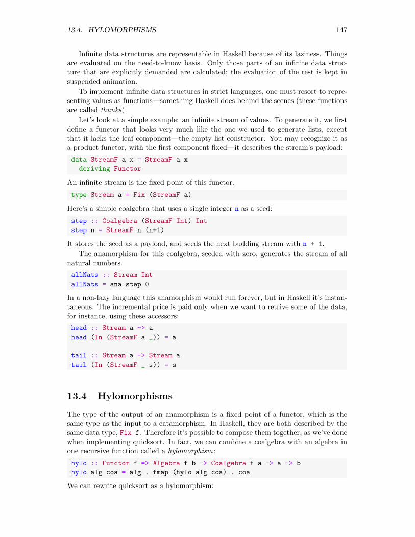
13.4. HYLOMORPHISMS 147

Infinite data structures are representable in Haskell because of its laziness. Thingsare evaluated on the need-to-know basis. Only those parts of an infinite data struc-ture that are explicitly demanded are calculated; the evaluation of the rest is kept insuspended animation.

To implement infinite data structures in strict languages, one must resort to repre-senting values as functions—something Haskell does behind the scenes (these functionsare called thunks).

Let’s look at a simple example: an infinite stream of values. To generate it, we firstdefine a functor that looks very much like the one we used to generate lists, exceptthat it lacks the leaf component—the empty list constructor. You may recognize it asa product functor, with the first component fixed—it describes the stream’s payload:

data StreamF a x = StreamF a x

deriving Functor

An infinite stream is the fixed point of this functor.

type Stream a = Fix (StreamF a)

Here’s a simple coalgebra that uses a single integer n as a seed:

step :: Coalgebra (StreamF Int) Int

step n = StreamF n (n+1)

It stores the seed as a payload, and seeds the next budding stream with n + 1.

The anamorphism for this coalgebra, seeded with zero, generates the stream of allnatural numbers.

allNats :: Stream Int

allNats = ana step 0

In a non-lazy language this anamorphism would run forever, but in Haskell it’s instan-taneous. The incremental price is paid only when we want to retrive some of the data,for instance, using these accessors:

head :: Stream a -> a

head (In (StreamF a _)) = a

tail :: Stream a -> Stream a

tail (In (StreamF _ s)) = s

13.4 Hylomorphisms

The type of the output of an anamorphism is a fixed point of a functor, which is thesame type as the input to a catamorphism. In Haskell, they are both described by thesame data type, Fix f. Therefore it’s possible to compose them together, as we’ve donewhen implementing quicksort. In fact, we can combine a coalgebra with an algebra inone recursive function called a hylomorphism:

hylo :: Functor f => Algebra f b -> Coalgebra f a -> a -> b

hylo alg coa = alg . fmap (hylo alg coa) . coa

We can rewrite quicksort as a hylomorphism:


qsort = hylo toList split

Notice that there is no trace of the fixed point in the definition of the hylomorphism.Conceptually, the coalgebra is used to build (unfold) the recursive data structure fromthe seed, and the algebra is used to fold it into a value of type b. But because ofHaskell’s laziness, the intermediate data structure doesn’t have to be materialized infull in memory. This is particularly important when dealing with very large intermediatetrees. Only the branches that are currently being traversed are evaluated and, as soonas they have been processed, they are passed to the garbage collector.

Hylomorphisms in Haskell are a convenient replacement for recursive backtrackingalgorithms, which are very hard to implement correctly in imperative languages. Wetake advantage of the fact that designing a data structure is easier than followingcomplicated flow of control and keeping track of our place in a recursive algorithm.

This way, data structures can be used to visualize complex flows of control.

The impedance mismatch

We’ve seen that, in the category of sets, the initial algebras don’t necessarily coincidewith terminal coalgebras. The identity functor, for instance, has the empty set as thecarrier of the initial algebra and the singleton set as the carrier of its terminal coalgebra.

We have other functors that have no leaf components, such as the stream functor.The initial algebra for such a functor is the empty set as well.

In Set, the initial algebra is the subset of the terminal coalgebra, and hylomorphismscan only be defined for this subset. It means that we can use a hylomorphism only if theanamorphism for a particular coalgebra lands us in this subset. In that case, becausethe embedding of initial algebras in terminal coalgebras is injective, we can find thecorresponding element in the initial algebra and apply the catamorphism to it.

In Haskell, however, we have one type, Fix f, combining both, the initial algebraand the terminal coalgebra. This is where the simplistic interpretation of Haskell typesas sets of values breaks down.

Let’s consider this simple stream algebra:

add :: Algebra (StreamF Int) Int

add (StreamF n sum) = n + sum

Nothing prevents us from using a hylomorphism to calculate the sum of all naturalnumbers:

sumAllNats :: Int

sumAllNats = hylo add step 1

It’s a perfectly well-formed Haskell program that passes the type checker. So what valuedoes it produce when we run it? (Hint: It’s not −1/12.) The answer is: we don’t know,because this program never terminates. It runs into infinite recursion and eventuallyexhausts the computer’s resources.

This is the aspect of real-life computations that mere functions between sets cannotmodel. Some computer function may never terminate.

Recursive functions are formally described by domain theory as limits of partiallydefined functions. If a function is not defined for a particular value of the argument, it issaid to return a bottom value ⊥. If we include bottoms as special elements of every type(these are then called lifted types), we can say that our function sumAllNats returns a

13.5. TERMINAL COALGEBRA FROM UNIVERSALITY 149

bottom of the type Int. In general, catamorphisms for infinite types don’t terminate,so we can treat them as returning bottoms.

It should be noted, however, that the inclusion of bottoms complicates the categor-ical interpretation of Haskell. In particular, many of the universal constructions thatrely on uniqueness of mappings no longer work as advertised.

The “bottom” line is that Haskell code should be treated as an illustration of cate-gorical concepts rather than a source of rigorous proofs.

13.5 Terminal Coalgebra from Universality

The definition of an anamorphism can be seen as an expression of the universal propertyof the terminal coalgebra. Here it is, with the universal quantification made explicit:

ana :: Functor f => forall a. Coalgebra f a -> (a -> Fix f)

ana coa = In . fmap (ana coa) . coa

It says that, given any coalgebra, there is a mapping from its carrier to the carrier ofthe terminal coalgebra, Fix f. We know, from the Lambek’s lemma, that this mappingis in fact a coalgebra morphism.

Let’s uncurry this definition:

ana :: Functor f => forall a. (a -> f a, a) -> Fix f

ana (coa, x) = In (fmap (curry ana coa) (coa x))

In this form, we can take it as the definition of the carrier for the terminal coalgebra. Wecan replace Fix f with the type we are defining—let’s call it Nu f. The type signature:

forall a. (a -> f a, a) -> Nu f

tells us that we can construct an element of Nu f from a pair (a -> f a, a). It looksjust like a data constructor, except that it’s polymorphic in a.

Data types with a polymorphic constructor are called existential types. To constructan element of an existential type, we have the option of picking the most convenienttype—the type for which we have the data required by the constructor.

For instance, we can construct a term of the type Nu (StreamF Int) by pickingInt as the convenient type, and providing the pair:

nuArgs :: (Int -> StreamF Int Int, Int)

nuArgs = (\n -> StreamF n (n+1) , 0)

The clients of an existential data type have no idea what type was used in itsconstruction. All they know is that such a type exists—hence the name. If they wantto use an existential type, they have to do it in a way that is not sensitive to the choicethat was made in its construction. In practice, it means that an existential type mustcarry with itself both the producer and the consumer of the hidden value.

This is indeed the case in our example: the producer is just the value of type a, andthe consumer is the function a -> f a.

Naively, all that the clients could do with this pair, without any knowledge of whatthe type a was, is to apply the function to the value. But if f is a functor, they can domuch more. They can repeat the process by applying the lifted function to the contentsof f a, and so on. They end up with all the information that’s contained in the infinitestream.


There are several ways of defining existential data types in Haskell. We can use theuncurried version of the anamorphism directly as the data constructor:

data Nu f where

Nu :: forall a f. (a -> f a, a) -> Nu f

Notice that, in Haskell, if we explicitly quantify one type, all other type variables mustalso be quantified: here, it’s the type constructor f (however, Nu f is not existential inf, since it’s an explicit parameter).

We can also omit the quantification altogether:

data Nu f where

Nu :: (a -> f a, a) -> Nu f

This is because type variables that are not arguments to the type constructor areautomatically treated as existentials.

We can also use the more traditional form:

data Nu f = forall a. Nu (a -> f a, a)

(This one requires the quantification of a.)

Finally, although this syntax is not allowed in Haskell, it’s often more intuitive towrite it like this:

data Nu f = Nu (exists a. (a -> f a, a))

(Later we’ll see that existential data types correspond to coends in category theory.)

The constructor of Nu f is literally the (uncurried) anamorphism:

anaNu :: Coalgebra f a -> a -> Nu f

anaNu coa a = Nu (coa, a)

If we are given a stream in the form of Nu (Stream a), we can access its elementusing accessors functions. This one extracts the first element:

head :: Nu (StreamF a) -> a

head (Nu (unf, s)) =

let (StreamF a _) = unf s

in a

and this one advances the stream:

tail :: Nu (StreamF a) -> Nu (StreamF a)

tail (Nu (unf, s)) =

let (StreamF _ s') = unf s

in Nu (unf, s')

You can test them on an infinite stream of integers:

allNats = Nu nuArgs

13.6 Terminal Coalgebra as a Limit

In category theory we are not afraid of infinitities—we make sense of them.

At face value, the idea that we could construct a terminal coalgebra by applying thefunctor F infinitely many times to some object, let’s say the terminal object 1, makesno sense. But the idea is very convincing: Applying F one more time is like adding one

13.6. TERMINAL COALGEBRA AS A LIMIT 151

to infinity—it’s still infinity. So, naively, this is a fixed point of F :

F (F∞1) ∼= F∞+11 ∼= F∞1

To turn this loose reasoning into a rigorous proof, we have to tame the infinity,which means we have to define some kind of a limiting procedure.

As an example, let’s consider the product functor:

Fax = a× x

Its terminal coalgebra is an infinite stream. We’ll approximate it it by starting withthe terminal object 1. The next step is:

Fa1 = a× 1 ∼= a

which we could imagine is a stream of length one. We can continue with:

Fa(Fa1) = a× (a× 1) ∼= a× a

a stream of length two, and so on.This looks promising, but what we need is one object that would combine all these

approximations. We need a way to glue the next approximation to the previous one.Recall, from an earlier exercise, the limit of the “walking arrow” diagram. This limit

has the same elements as the starting object in the diagram. In particular, consider thelimit in this diagram:

LimD1

1 F1

π0 π1

!

(! is the unique morphism targeting the terminal object 1). This limit has the sameelements as F1. Similarly, this limit:

LimD2

1 F1 F (F1)

π0π1

π2

! F !

has the same elements as F (F1).We can continue extending this diagram to infinity. The limit of the infinite chain

is the fixed point carrier of the terminal coalgebra.

t

1 F1 F (F1) ... Fn1 ...

π0π1

π2πn

! F ! F (F !) Fn!

The proof of this fact can be obtained from the analogous proof for initial algebras byreversing the arrows.

Chapter 14

Monads

What do a wheel, a clay pot, and a wooden house have in common? They are all usefulbecause of the emptiness in their center.

Lao Tzu says: “The value comes from what is there, but the use comes from whatis not there.”

What does the Maybe functor, the list functor, and the reader functor have in com-mon? They all have emptiness in their center.

When monads are explained in the context of programming, it’s hard to see thecommon pattern when you focus on the functors. To understand monads you have tolook inside functors and in between functions.

14.1 Programming with Side Effects

So far we’ve been talking about programming in terms of computations that weremodeled mainly on functions between sets (with the exception of non-termination). Inprogramming, such functions are called total and pure.

A total function is defined for all values of its arguments.

A pure function is implemented purely in terms of its arguments—it has no accessto, much less having the ability to modify, its environment.

Most real-world programs, though, have to interact with the external world: theyread and write files, process network packets, prompt users for data, etc. Most pro-gramming languages solve this problem by allowing side effect. A side effect is anythingthat breaks the totality or the purity of a function.

Unfortunately, this shotgun approach adopted by imperative languages makes rea-soning about programs extremely hard. When composing effectful computations onehas to carefully reason about the composition of effects, on a case-by-case basis. Tomake things even harder, most effects are hidden inside the implementation of a functionand all the functions it’s calling, recursively.

The solution adopted by purely functional languages, like Haskell, is to encode sideeffects in the return type of a pure function. Amazingly, this is possible for all relevanteffects.

The idea is that, instead of a computation of the type a->b with side effects, we usea function a -> f b, where the type constructor f encodes the appropriate effect. At

153

154 CHAPTER 14. MONADS

this point there are no conditions imposed on f. It doesn’t even have to be a Functor,much less a monad. This will come later, when we talk about effect composition.

Below is the list of common effects and their pure-function versions.

Partiality

In imperative languages, partiality is often encoded using exceptions. When a functionis called with the “wrong” value for its argument, it throws an exception. In somelanguages, the type of exception is encoded in the signature of the function using specialsyntax.

In Haskell, a partial computation can be implemented by a function returning theresult inside the Maybe functor. Such a function, when called with the “wrong” argu-ment, returns Nothing, otherwise is wraps the result in the Just constructor.

If we want to encode more information about the type of the failure, we can usethe Either functor, with the Left traditionally passing the error data (often a simpleString); and Right encapsulating the real return, if available.

The caller of a Maybe-valued function cannot easily ignore the exceptional condition.In order to extract the value, they have to pattern-match the result and decide how todeal with Nothing. This is in contrast to the “poor-man’s Maybe” of some imperativelanguages where the error condition is encoded using a null pointer.

Logging

Sometimes a computation has to log some values in some external data structure.Logging or auditing is a side effect that’s particularly dangerous in concurrent programs,where multiple threads might try to access the same log simultaneously.

The simple solution is for a function to return the computed value paired with theitem to be logged. In other words, a logging computation of the type a -> b can bereplaced by a pure function:

a -> Writer w b

where the Writer functor is a thin encapsulation of the product:

newtype Writer w a = Writer (a, w)

with w being the type of the log.

The caller of this function is then responsible for extracting the value to be logged.This is a common trick: make the function provide all the data, and let the caller dealwith the effects.

Environment

Some computations need read-only access to some external data stored in the environ-ment. The read-only environment, instead of being secretly accessed by a computation,can be simply passed to a function as an additional argument. If we have a computa-tion a -> b that needs access to some environment e, we replace it with a function(a, e) -> b. At first, this doesn’t seem to fit the pattern of encoding side effects in

the return type. However, such a function can always be curried to the form:

a -> (e -> b)

14.1. PROGRAMMING WITH SIDE EFFECTS 155

The return type of this function can be encoded in the reader functor, itself parame-terized by the environment type e:

newtype Reader e a = Reader (e -> a)

This is an example of a delayed side effect. The function:

a -> Reader e a

doesn’t want to deal with effects so it delegates the responsibility to the caller. Youmay think of it as producing a script to be executed at a later time. The functionrunReader plays the role of a very simple interpreter of this script:

runReader :: Reader e a -> e -> a

runReader (Reader h) e = h e

State

The most common side effect is related to accessing and potentially modifying someshared state. Unfortunately, shared state is the notorious source of concurrency errors.This is a serious problem in object oriented languages where stateful objects can betransparently shared between many clients. In Java, such objects may be providedwith individual mutexes at the cost of impaired performance and the risk of deadlocks.

In functional programming we make state manipulations explicit: we pass the stateas an additional argument and return the modified state paired with the return value.We replace a stateful computation a -> b with

(a, s) -> (b, s)

where s is the type of state. As before, we can curry such a function to get it to theform:

a -> (s -> (b, s))

This return type can be encapsulated in the following functor:

newtype State s a = State (s -> (a, s))

The caller of such a function is supposed to retrieve the result and the modified stateby providing the initial state and calling the helper function, the interpreter, runState:

runState :: State s a -> s -> (a, s)

runState (State h) s = h s

Notice that, modulo constructor unpacking, runState is bona fide function application.

Nondeterminism

Imagine performing a quantum experiment that measures the spin of an electron. Halfof the time the spin will be up, and half of the time it will be down. The result isnon-deterministic. One way to describe it is to use the many-worlds interpretation:when we perform the experiment, the Universe splits into two universes, one for eachresult.

What does it mean for a function to be non-deterministic? It means that it willreturn different results every time it’s called. We can model this behavior using themany-worlds interpretation: we let the function return all possible results at once. Inpractice, we’ll settle for a (possibly infinite) list of results:


We replace a non-deterministic computation a -> b with a pure function returninga functor-ful of results—this time it’s the list functor:

a -> [b]

Again, it’s up to the caller to decide what to do with these results.

Input/Output

This is the trickiest side effect because it involves interacting with the external world.Obviously, we cannot model the whole world inside a computer program. So, in orderto keep the program pure, the interaction has to happen outside of it. The trick isto let the program generate a script. This script is then passed to the runtime to beexecuted. The runtime is the effectful virtual machine that runs the program.

This script itself sits inside the opaque, predefined IO functor. The values hidden inthis functor are not accessible to the program: there is no runIO function. Instead, theIO value produced by the program is executed, at least conceptually, after the programis finished.

In reality, because of Haskell’s laziness, the execution of I/O is interleaved withthe rest of the program. Pure functions that comprise the bulk of your program areevaluated on demand—the demand being driven by the execution of the IO script. Ifit weren’t for I/O, nothing would ever be evaluated.

The IO object that is produced by a Haskell program is called main and its typesignature is:

main :: IO ()

It’s the IO functor containing the unit—meaning: there is no useful value other thanthe input/output script.

We’ll talk about how IO actions are created soon.

Continuation

We’ve seen that, as a consequences of the Yoneda lemma, we can replace a value oftype a with a function that takes a handler for that value. This handler is called acontinuation. Calling a handler is considered a side effect of a computation. In termsof pure functions, we encode it as:

a -> Cont r b

where Cont r is the following functor:

newtype Cont r a = Cont ((a -> r) -> r)

It’s the responsibility of the caller of this function to provide the continuation andretrieve the result:

runCont :: Cont r a -> (a -> r) -> r

runCont (Cont f) k = f k

This is the Functor instance for Cont r:

instance Functor (Cont r) where

-- f :: a -> b

-- k :: b -> r

fmap f c = Cont (\k -> runCont c (k . f))

14.2. COMPOSING EFFECTS 157

Notice that this is a covariant functor because the type a is in a doubly negative position.

14.2 Composing Effects

Now that we know how to make one giant leap using a function that produces both avalue and a side effect, the next problem is to figure out how to decompose this leapinto smaller human-sized steps. Or, conversely, how to combine two smaller steps intoone larger step.

The way effectful computations are composed in imperative languages is to useregular function composition for the values and let the side effects combine themselvesseparately.

When we represent effectful computations as pure functions, we are faced with theproblem of composing two functions of the form

g :: a -> f b

h :: b -> f c

In all cases of interest the type constructor f happens to be a Functor, so we’ll assumethat in what follows.

The naive approach would be to unpack the result of the first function, pass thevalue to the next function, then compose the effects of both functions on the side, andcombine them with the result of the second function. This is not always possible, evenfor cases that we have studied so far, much less for an arbitrary type constructor.

It’s instructive to see how we could do it for the Maybe functor. If the first functionreturns Just, we pattern match it to extract the contents and call the next functionwith it.

But if the first function returns Nothing, we have no value with which to callthe second function. We have to short-circuit it, and return Nothing directly. Socomposition is possible, but it means modifying flow of control by skipping the secondcall based on the side effect of the first call.

For some functors the composition of side effects is possible, for others it’s not. Howcan we characterize those “good” functors?

For a functor to encode composable side effects we must at least be able to implementthe following polymorphic higher-order function:

composeWithEffects :: Functor f =>

(b -> f c) -> (a -> f b) -> (a -> f c)

This is very similar to regular function composition:

(.) :: (b -> c) -> (a -> b) -> (a -> c)

so it’s natural to ask if there is a category in which the former defines a composition ofarrows. Let’s see what more is needed to construct such a category.

Objects in this new category are the same Haskell types as before. But an arrowfrom a to b is implemented as a Haskell function:

g :: a -> f b

Our composeWithEffects can then be used to implement the composition of sucharrows.


To have a category, we require that this composition be associative. We also needan identity arrow for every object a. This is an arrow from a to a, so it corresponds toa Haskell function:

idWithEffects :: a -> f a

It must behave like identity with respect to composeWithEffects.

We have just defined a monad! After some renaming and rearranging, we can writeit as a typeclass:

class Functor m => Monad m where

(<=<) :: (b -> m c) -> (a -> m b) -> (a -> m c)

return :: a -> m a

The infix operator <=< replaces the function composeWithEffects. The return func-tion is the identity arrow in our new category. (This is not the definition of the monadyou’ll find in the Haskell’s Prelude but, as we’ll see soon, it’s equivalent to it.)

As an exercise, let’s define the Monad instance for Maybe. The “fish” operator <=<

composes two functions:

f :: a -> Maybe b

g :: b -> Maybe c

into one function of the type a -> Maybe c. The unit of this composition, return,encloses a value in the Just constructor.

instance Monad Maybe where

g <=< f = \a -> case f a of

Nothing -> Nothing

Just b -> g b

return = Just

You can easily convince yourself that category laws are satisfied. In particularreturn <=< g is the same as g and f <=< return is the same as f. The proof of

associativity is also pretty straightforward: If any of the functions returns Nothing, theresult is Nothing; otherwise it’s just a straightforward function composition, which isassociative.

The category that we have just defined is called the Kleisli category for the monadm. The functions a -> m b are called the Kleisli arrows. They compose using <=< andthe identity arrow is called return.

All functors from the previous section are Monad instances. If you look at them astype constructors, or even functors, it’s hard to see any similarities between them. Thething they have in common is that they can be used to implement composable Kleisliarrows.

As Lao Tze would say: Composition is something that happens between things.While focusing our attention on things, we often lose sight of what’s in the gaps.

14.3 Alternative Definitions

The definition of a monad using Kleisli arrows has the advantage that the monad lawsare simply the associativity and the unit laws of a category. There are two other equiva-lent definitions of a monad, one preferred by mathematicians, and one by programmers.

14.3. ALTERNATIVE DEFINITIONS 159

First, let’s notice that, when implementing the fish operator, we are given twofunctions as arguments. The only thing a function is useful for is to be applied to anargument. When we apply the first function f :: a -> m b we get a value of thetype m b. At this point we would be stuck, if it weren’t for the fact that m is a functor.Functoriality lets us apply the second function g :: b -> m c to m b. Indeed thelifting of g by m is of the type:

m b -> m (m c)

This is almost the result we are looking for, if we could only flatten m(m c) to m c.This flattening is called join. In other words, if we are given:

join :: m (m a) -> m a

we can implement <=<:

g <=< f = \a -> join (fmap g (f a))

or, using point free notation:

g <=< f = join . fmap g . f

Conversely, join can be implemented in terms of <=<:

join = id <=< id

This may not be immediately obvious, until you realize that the rightmost id is applidedto m (m a), and the leftmost is applied to m a. We interpret a Haskell function:

m (m a) -> m (m a)

as an arrow in the Kleisli category that goes from m(m a) to m a. Similarly, thefunction:

m a -> m a

implements a Kleisli arrow from m a to a. Their Kleisli composition produces a Kleisliarrow from m (m a) to a, or a Haskell function:

m (m a) -> m a

This leads us to the equivalent definition of a monad in terms of join and return:



return :: a -> m a

This is still not the definition you will find in the standard Haskell Prelude. Sincethe fish operator is a generalization of the dot operator, using it is equivalent to point-free programming. It lets us compose arrows without naming intermediate values.Although some consider point-free programs more elegant, most programmers find themdifficult to follow.

But function composition is really done in two steps: We apply the first function,then apply the second function to the result. Explicitly naming the intermediate resultis often helpful in understanding of what’s going on.

To do the same with Kleisli arrows, we have to know how to apply the second Kleisliarrow to a named monadic value—the result of the first Kleisli arrow. The functionthat does that is called bind and is written as an infix operator:


(>>=) :: m a -> (a -> m b) -> m b

Obviously, we can implement Kleisli composition in terms of bind:

g <=< f = \a -> (f a) >>= g

Conversely, bind can be implemented in terms of the Kleisli arrow:

ma >>= k = (k <=< id) ma

This leads us to the following definition:

class Monad m where

(>>=) :: m a -> (a -> m b) -> m b

return :: a -> m a

This is almost the definition you’ll find in the Prelude, except for the additional con-straint. This constraint states the fact that every instance of Monad is also an instanceof Applicative. We will postpone the discussion of applicatives to the section onmonoidal functors.

We can also implement join using bind:

join :: (Monad m) => m (m a) -> m a

join mma = mma >>= id

Here, id goes from m a to m a or, as a Kleisli arrow, from m a to a.Interestingly, a Monad defined using bind is automatically a functor. The lifting

function for it is called liftM

liftM :: Monad m => (a -> b) -> (m a -> m b)

liftM f ma = ma >>= (return . f)

14.4 Monad Instances

We are now ready to define monad instances for the functors we used to describe sideeffects. This will allow us to compose side effects.

Partiality

We’ve already seen the version of the Maybe monad implemented using Kleisli compo-sition. Here’s the more familiar implementation using bind:

instance Monad Maybe where

Nothing >>= k = Nothing

(Just a) >>= k = k a

return = Just

Logging

In order to compose functions that produce logs, we need a way to combine individuallog entries. This is why the writer monad:

newtype Writer w a = Writer (a, w)

requires the type of the log to be an instance of Monoid. This allows us to append logsand to create an empty log.

14.4. MONAD INSTANCES 161

instance Monoid w => Monad (Writer w) where

(Writer (a, w)) >>= k = let (Writer (b, w')) = k a

in Writer (b, mappend w w')

return a = Writer (a, mempty)

The let clause is used for introducing local bindings. Here, the result of applying k ispattern matched, and the local variables b and w' are initialized. The let/in constructis an expression whose value is given by the content of the in clause.

Environment

The reader monad is a thin encapsulation of a function from the environment to thereturn type:

newtype Reader e a = Reader (e -> a)

Here’s the Monad instance:

instance Monad (Reader e) where

ma >>= k = Reader (\e -> let a = runReader ma e

in runReader (k a) e)

return a = Reader (\e -> a)

The implementation of bind for the reader monad creates a function that takes theenvironment as its argument. This environment is used twice, first to run ma to get thevalue of a, and then to evaluate the value produced by k a.

The implementation of return ignores the environment.

Exercise 14.4.1. Define the Functor and the Monad instance for the following datatype:

newtype E e a = E (e -> Maybe a)

Hint: You may use this handy function:

runE :: E e a -> e -> Maybe a

runE (E f) e = f e

State

Like reader, the state monad is a function type:


Its bind is similar, except that the result of k acting on a is now run with the modifiedstate s'.

instance Monad (State s) where

st >>= k = State (\s -> let (a, s') = runState st s

in runState (k a) s')

return a = State (\s -> (a, s))

Applying bind to identity gives us the definition of join:


join :: State s (State s a) -> State s a

join mma = State (\s -> let (ma, s') = runState mma s

in runState ma s')

Notice that we are essentially passing the result of the first runState to the secondrunState, except that we have to uncurry the second one so it can accept a pair:

join mma = State (\s -> (uncurry runState) (runState mma s))

In this form, it’s easy to convert it to point-free notation:

join mma = State (uncurry runState . runState mma)

There are two basic Kleisli arrows (the first one, conceptually, coming from theterminal object ()) with which we can construct an arbitrary stateful computation.The first one retrieves the current state:

get :: State s s

get = State (\s -> (s, s))

and the second one modifies it:

set :: s -> State s ()

set s = State (\_ -> ((), s))

Nondeterminism

For the list monad, let’s consider how we could implement join. It must turn a list oflists into a single list. This can be done by concatenating all the inner lists using thelibrary function concat. From there, we can derive the implementation of bind.

instance Monad [] where

as >>= k = concat (fmap k as)

return a = [a]

return constructs a singleton list.

What in imperative languages do using nested loops we can do in Haskell using thelist monad. Think of as as aggregating the result of running the inner loop and k asthe code that runs in the outer loop.

In many ways, Haskell’s list behaves more like what is called an iterator or a gen-erator in imperative languages. Because of laziness, the elements of the list are rarelystored in memory all at once. You may also think of a list as a coroutine that produces,on demand, elements of a sequence.

Continuation

The implementation of bind for the continuation monad:

newtype Cont r a = Cont ((a -> r) -> r)

requires some backward thinking, because of the inherent inversion of control—the“don’t call us, we’ll call you” principle.

The result of bind is supposed to be a function that takes, as an argument, acontinuation k of the type:

14.5. DO NOTATION 163

k :: b -> r

We have to put together such a function given the two ingredients at our disposal:

ma :: Cont r a

fk :: a -> Cont r b

We’d like to run ma, but for that we need a continuation that would accept an a. Wecan build such a continuation: given an a it would call fk. The result is a b-expectingcontinuation Cont r b. But that’s exactly the continuation k we have at our disposal.Taken together, this convoluted process produces the following implementation:

instance Monad (Cont r) where

ma >>= fk = Cont (\k -> runCont ma (\a -> runCont (fk a) k))

return a = Cont (\k -> k a)

As we mentioned earlier, composing continuations is not for the faint of heart. However,it has to be implemented only once—in the definition of the continuation monad. Fromthere on, the do notation will make the rest relatively easy.

Input/Output

The IO monad’s implementation is baked into the language. The basic I/O primitivesare available through the library. They are either in the form of Kleisli arrows, or IO

objects (conceptually, Kleisli arrows from the terminal object ()).

For instance, the following object contains a command to read a line from thestandard input:

getLine :: IO String

There is no way to extract the string from it, since it’s not there yet; but the programcan process it through a further series of Kleisli arrows.

The IO monad is the ultimate procrastinator: the composition of its Kleisli arrowspiles up task after task to be executed later by the Haskell runtime.

To output a string followed by a newline, you can use this Kleisli arrow:

putStrLn :: String -> IO ()

Combining the two, you may construct a simple main object:

main :: IO ()

main = getLine >>= putStrLn

which echos a string you type.

14.5 Do Notation

It’s worth repeating that the sole purpose of monads in programming is to let us de-compose one big Kleisli arrow into multiple smaller ones.

This can be either done directly, in a point-free style, using Kleisli composition <=<;or by naming intermediate values and binding them to Kleisli arrows using >>=.

Some Kleisli arrows are defined in libraries, others are reusable enough to warrantout-of-line implementation but, in practice, the majority are implemented as single-shotinline lambdas.

Here’s a simple example:


main :: IO ()

main =

getLine >>= \s1 ->

getLine >>= \s2 ->

putStrLn ("Hello " ++ s1 ++ " " ++ s2)

which uses an ad-hoc Kleisli arrow of the type String->IO () defined by the lambdaexpression:

\s1 ->

getLine >>= \s2 ->


The body of this lambda is further decomposed using another ad-hoc Kleisli arrow:

\s2 -> putStrLn ("Hello " ++ s1 ++ " " ++ s2)

Such constructs are so common that there is special syntax called the do notationthat cuts through a lot of boilerplate. The above code, for instance, can be written as:

main = do

s1 <- getLine

s2 <- getLine


The compiler will automatically convert it to a series of nested lambdas. The lines1<-getLine is usually read as: “s1 gets the result of getLine.”

Here’s another example: a function that uses the list monad to generate all possiblepairs of elements taken from two lists.

pairs :: [a] -> [b] -> [(a, b)]

pairs as bs = do

a <- as

b <- bs

return (a, b)

Notice that the last line in a do block must produce a monadic value—here this isaccomplished using return.

As mentioned before, the do notation makes an easy task of otherwise very cum-bersome composition of continuations.

Most imperative languages lack the abstraction power to generically define a monadand instead they attempt to hard-code some of the more common monads. For instance,they implement exceptions as an alternative to the Either monad, or concurrent tasksas an alternative to the continuation monad. Some, like C++, introduce coroutinesthat mimic Haskell’s do notation.

Exercise 14.5.1. Implement the following function that works for any monad:

ap :: Monad m => m (a -> b) -> m a -> m b

Hint: Use do notation to extract the function and the argument. Use return to returnthe result.

Exercise 14.5.2. Rewrite the pairs function using the bind operators and lambdas.

14.6. MONADS CATEGORICALLY 165

14.6 Monads Categorically

In category theory monads first arose in the study of algebras. In particular, we canuse the bind operator to implement the very important operation of substitution.

Substitution

Consider this simple expression type. It’s parameterized by the type x that we can usefor naming variables:

data Ex x = Val Int

| Var x

| Plus (Ex x) (Ex x)

deriving (Functor, Show)

We can, for instance, construct an expression (2 + a) + b:

ex :: Ex Char

ex = Plus (Plus (Val 2) (Var 'a')) (Var 'b')

We can implement the Monad instance for Ex:

instance Monad Ex where

Val n >>= k = Val n

Var x >>= k = k x

Plus e1 e2 >>= k =

let x = e1 >>= k

y = e2 >>= k

in (Plus x y)

return x = Var x

Now suppose that you want to make a substitution by replacing a with x1 + 2 andb with x2 (for simplicity, let’s not worry about other letters of the alphabet). Thissubstitution is represented by the Kleisli arrow sub (as you can see, we are even ableto change the type of variable names from Char to String):

sub :: Char -> Ex String

sub 'a' = Plus (Var "x1") (Val 2)

sub 'b' = Var "x2"

When we bind it to ex

ex' :: Ex String

ex' = ex >>= sub

we get, as expected, a tree corresponding to (2 + (x1 + 2)) + x2.

Monad as a monoid

Let’s analyze the definition of a monad that uses join:



return :: a -> m a

We have an endofunctor m and two polymorphic functions.


In category theory, the functor that defines the monad is traditionally denoted byT (probably because monads were initially called “triples”). The two polymorphicfunctions become natural transformations. The first one, corresponding to join, mapsthe “square” of T—or a composition of T with itself—to T :

µ : T ◦ T → T

(Of course, only endo-functors can be squared this way.)The second, corresponding to return, maps the identity functor to T :

η : Id→ T

Compare this with our earlier definition of a monoid in a monoidal category:

µ : m⊗m→ m

η : i→ m

The similarity is striking. This is why we often call the natural transformation µmonadic multiplication. But in what category can the composition of functors be con-sidered a tensor product?

Enter the category of endofunctors. Objects in this category are endofunctors andarrows are natural transformations.

But there’s more structure to that category. Any two endofunctors can be com-posed, so maybe composition could be considered a tensor product? After all, the onlycondition we impose on a tensor product is that it’s functorial in both arguments. Thatis, given a pair of arrows:

α : T → T ′

β : S → S′

we can lift it to the mapping of the tensor product:

α⊗ β : T ⊗ S → T ′ ⊗ S′

In the category of endofunctors, the arrows are natural transformations so, if wereplace ⊗ with ◦, the lifting would be a mapping:

α ◦ β : T ◦ T ′ → S ◦ S′

But this is just the horizontal composition of natural transformations (now you under-stand why it’s denoted by a circle).

The unit object in this monoidal category is the identity endofunctor, and unit lawsare satisfied “on the nose,” meaning

Id ◦ T = T = T ◦ Id

We don’t need any unitors. We don’t need any associators either, since functor compo-sition is automatically associative.

A monoidal category in which unit and associativity laws are equalities is called astrict monoidal category.

14.7. FREE MONADS 167

Notice, however, that composition is not symmetric, so this is not a symmetricmonoidal category.

So, all said, a monad is a monoid in the monoidal category of endofunctors.

A monad (T, η, µ) consists of an object in the category of endofunctors—meaningan endofunctor T ; and two arrows—meaning natural transformations:

η : Id→ T

µ : T ◦ T → T

For this to be a monoid, these arrows must satisfy monoidal laws. Here are the unitlaws (with unitors replaced by strict equalities):

Id ◦ T T ◦ T T ◦ Id

T

η◦T

=µ

T◦η

=

and this is the associativity law:

(T ◦ T ) ◦ T T ◦ (T ◦ T )

T ◦ T T ◦ T

T

=

µ◦T T◦µ

µ µ

We used the whiskering notation for horizontal composition of µ ◦ T and T ◦ µ.

These are the monad laws in terms of µ and η. They can be directly translatedto the laws for join and return. They are also equivalent to the laws of the Kleislicategory built from arrows a→ Tb.

14.7 Free Monads

A monad is an endofunctor T : [C, C] equipped with additional structure given by twonatural transformations. This kind of statement can be made precise by defining aforgetful functor that ignores the additional structure. In our case, we would take amonad (T, η, µ) and keep only T . But in order to define a functor, we first need todefine the category of monads.

Category of monads

The objects in the category of monads Mon(C) are monads (T, η, µ). We can define anarrow between two monads (T, η, µ) and (T ′, η′, µ′) as a natural transformation betweenthe two endofunctors:

λ : T → T ′

However, since monads are endofunctors with structure, we want these natural trans-formations to preserve the structure. Preservation of unit means that the following


diagram must commute:

Id

T T ′η

η′

λ

Preservation of multiplication means that the following diagram must commute:

T ◦ T T ′ ◦ T ′

T T ′

λ◦λ

µ µ′

λ

Another way of looking at Mon(C) is that it’s a category of monoids in [C, C].

Free monad

Now that we have a category of monads, we can define the forgetful functor:

U : Mon(C)→ [C, C]

that maps (T, η, µ) to T and a monad morphism to the underlying natural transforma-tion.

We would like a free monad to be generated by a left adjoint to this forgetful functor.The problem is that this left adjoint doesn’t always exist. So far we’ve been avoidingtalking about sizes of sets, and it was okay. Unfortunately, monads tend to blow thingsup. The bottom line is that free monads exist for some, but not all, endofunctors.Therefore we can’t define a free monad through an adjunction. Fortunately, in cases ofinterest a free monad can be defined as a fixed point of an algebra.

The construction is analogous to how we defined a free monoid as an initial algebrafor the list functor:

data ListF a x = NilF | ConsF a x

or the more general:

Fax = I + a⊗ x

This time, however, the monoidal category in which a monad is defined as a monoid isthe category of endofunctors ([C, C], Id, ◦). A free monoid in this category is the initialalgebra for the “list” functor that maps functors to functors:

ΦFG = Id + F ◦G

Here, the coproduct of two functors is defined point-wise. On objects:

(F +G)a = Fa+Ga

and on arrows:

(F +G)f = Ff +Gf

(We can form a coproduct of two morphisms using the functoriality of the coproduct.We are assuming that C is co-cartesian, that is all coproducts exist.)


The initial algebra is the (least) fixed point of this operator, or the solution to theidentity:

LF ∼= Id + F ◦ LFThis formula establishes a natural isomorphism between two functors. In particular,the mapping out of the sum is equivalent to a pair of natural transformations:

Id→ LF

F ◦ LF → LF

When translating to Haskell, the components of these transformation become two con-structors. We get the following data type parameterized by a functor f:

data FreeMonad f a where

Pure :: a -> FreeMonad f a

Free :: f (FreeMonad f a) -> FreeMonad f a

If we think of a functor f as a container of values, the constructor Free takes acontainer of (FreeMonad f a) and stashes it away. An arbitrary value of the typeFreeMonad f a is therefore a tree in which every node is a functorful of branches, andeach leaf contains a value of the type a.

Because this definition is recursive, the Functor instance for it is also recursive:

instance Functor f => Functor (FreeMonad f) where

fmap g (Pure a) = Pure (g a)

fmap g (Free ffa) = Free (fmap (fmap g) ffa)

The outer fmap uses the Functor instance of f, while the inner (fmap g) recurses intothe branches.

The monadic unit is just a thin encapsulation of the identity functor:

eta :: a -> FreeMonad f a

eta a = Pure a

Monadic multiplication, or join, is defined recursively:

mu :: Functor f => FreeMonad f (FreeMonad f a) -> FreeMonad f a

mu (Pure fa) = fa

mu (Free ffa) = Free (fmap mu ffa)

The Monad instance for FreeMonad f is therefore:

instance Functor f => Monad (FreeMonad f) where

return a = eta a

m >>= k = mu (fmap k m)

We can also define bind directly:

(Pure a) >>= k = k a

(Free ffa) >>= k = Free (fmap (>>= k) ffa)

A free monad accumulates monadic actions in a tree-like structure without com-mitting to a particular evaluation strategy. This tree can be “interpreted” using analgebra. This time it’s an algebra in the category of endofunctors, so its carrier is anendofunctor G and the structure map is a natural transformation:

α : I + F ◦G→ G


This natural transformation, being a mapping out of a sum, is equivalent to a pair ofnatural transformations:

λ : I → G

ρ : F ◦G→ G

We can translate it to Haskell as a pair of polymorphic functions corresponding toλ and ρ:

type MAlg f g a = (a -> g a, f (g a) -> g a)

Since the free monad is the initial algebra, there is a unique mapping—the catamorphism—from it to any other algebra. Recall how we defined a catamorphism for a regularalgebra:

cata :: Functor f => Algebra f a -> Fix f -> a


The out part exposes the contents of the fixed point. Here we can do this by pattern-matching on the two constructors of the free monad. If it’s a leaf, we apply our λ to it.If it’s a node, we recursively process its contents, and apply our ρ to the result:

mcata :: Functor f => MAlg f g a -> FreeMonad f a -> g a

mcata (l, r) (Pure a) = l a

mcata (l, r) (Free ffa) =

r (fmap (mcata (l, r)) ffa)

Exercise 14.7.1. A rose tree is defined as

data Rose a = Leaf a | Rose [Rose a]

deriving Functor

Implement conversions back and forth between Rose a and FreeMonad [] a.

Stack calculator example

As an example, let’s consider a stack calculator implemented as an embedded domain-specific language, EDSL. We’ll use the free monad to accumulate simple commandswritten in this language.

The commands are defined by the functor StackF. Think of the parameter k as thecontinuation.

data StackF k = Push Int k

| Top (Int -> k)

| Pop k

| Add k

deriving Functor

For instance, Push is supposed to push an integer on the stack and then call the con-tinuation k.

The free monad for this functor can be thought of as a tree, with most brancheshaving just one child, thus forming lists. The exception is the Top node, which hasmany children, one per every value of Int.

This is the free monad for this functor:


type FreeStack = FreeMonad StackF

In order to create domain-specific programs we’ll define a few helper functions.There is a generic one that lifts a functorful of values to a free monad:

liftF :: (Functor f) => f r -> FreeMonad f r

liftF fr = Free $ fmap (Pure) fr

We also need a series of “smart constructors,” which are Kleisli arrows for our freemonad:

push :: Int -> FreeStack ()

push n = liftF (Push n ())

pop :: FreeStack ()

pop = liftF (Pop ())

top :: FreeStack Int

top = liftF (Top id)

add :: FreeStack ()

add = liftF (Add ())

Since a free monad is a monad, we can conveniently combine Kleisli arrows usingthe do notation. For instance, here’s a toy program that adds two numbers and returnstheir sum:

calc :: FreeStack Int

calc = do

push 3

push 4

add

x <- top

pop

return x

In order to execute this program, we need to define an algebra whose carrier is anendofunctor. Since we want to implement a stack-based calculator, we’ll use a versionof a state functor whose state is a stack—a list of integers. It’s a function type thattakes a list and returns a new list coupled with the continuation:

data StackAction k = St ([Int] -> ([Int], k))

deriving Functor

To run the action, we apply the continuation to the stack:

runAction :: StackAction k -> [Int] -> ([Int], k)

runAction (St k) ns = k ns

We define the algebra as a pair of polymorphic functions corresponding to the twoconstructors of the free monad:

runAlg :: MAlg StackF StackAction a

runAlg = (stop, go)

The first function terminates the execution of the program and returns a value:


stop :: a -> StackAction a

stop a = St (\xs -> (xs, a))

The second function pattern matches on the type of the command. Each commandcarries with it a continuation. This continuation has to be run with a modified stack.Each command modifies the stack in a different way:

go :: StackF (StackAction k) -> StackAction k

go (Pop k) = St (\ns -> runAction k (tail ns))

go (Top ik) = St (\ns -> runAction (ik (head ns)) ns)

go (Push n k) = St (\ns -> runAction k (n: ns))

go (Add k) = St (\ns -> runAction k

((head ns + head (tail ns)): tail (tail ns)))

For instance, Pop discards the top of the stack. Top takes an integer from top of thestack and uses it to pick the branch to be executed. It does it by applying the functionik to the integer. Add adds the two numbers at the top of the stack and pushes theresult.

Notice that the algebra we have defined does not involve recursion. Separatingrecursion from the actions is one of the advantages of the free monad approach. Therecursion is instead encoded once and for all in the catamorphism.

Here’s the function that can be used to run our toy program:

run :: FreeMonad StackF k -> ([Int], k)

run prog = runAction (mcata runAlg prog) []

Obviously, the use of partial functions head and tail makes our interpreter fragile.A badly formed program will cause a runtime error. A more robust implementationwould use an algebra that allows for error propagation.

The other advantage is that the same program may be interpreted using differentalgebras.

Exercise 14.7.2. Implement a “pretty printer” that displays the program constructedusing our free monad. Hint: Implement the algebra that uses the Const functor as thecarrier:

showAlg :: MAlg StackF (Const String) a

14.8 Monoidal Functors

We’ve seen several examples of monoidal cateogries. Such categories are equipped withsome kind of binary operation, e.g., a cartesian product, a sum, composition (in thecategory of endofunctors), etc. They also have a special object that serves as a unitwith respect to that binary operation. Unit and associativity laws are satisfied eitheron the nose (in strict monoidal categories) or up to isomorphism.

Every time we have more than one instance of some structure, we may ask ourselvesthe question: is there a whole category of such things? In this case: do monoidalcategories form their own category? For this to work we would have to define arrowsbetween monoidal categories.

A monoidal functor F from a monoidal category (C,⊗, i) to another monoidal cat-egory (D,⊕, j) maps tensor product to tensor product and unit to unit—all up to

14.8. MONOIDAL FUNCTORS 173

isomorphism:

Fa⊕ Fb ∼= F (a⊗ b)j ∼= Fi

Here, on the left-hand side we have the tensor product and the unit in the targetcategory, and on the right their counterparts in the source category.

If the two monoidal categories in question are not strict, that is the unit and as-sociativity laws are satisfied only up to isomorphism, there are additional coherencyconditions that ensure that unitors are mapped to unitors and associators are mappedto associators.

The category of monoidal categories with monoidal functors as arrows is calledMonCat. In fact it’s a 2-category, since one can define structure-preserving naturaltransformations between monoidal functors.

Lax monoidal functors

One of the perks of monoidal categories is that they allow us to define monoids. Youcan easily convince yourself that monoidal functors map monoids to monoids. It turnsout that you don’t need the full power of monoidal functors to accomplish this task.Let’s consider what the minimal requirements are for a functor to map a monoid to amonoid.

Let’s start with a monoid (m,µ, η) in the monoidal category (C,⊗, i). Consider afunctor F that maps m to Fm. We want Fm to be a monoid in the target monoidalcategory (D,⊕, j). For that we need to find two mappings:

η′ : j → Fm

µ′ : Fm⊕ Fm→ Fm

satisfying monoidal laws.Since m is a monoid, we do have at our disposal the liftings of the original mappings:

Fη : Fi→ Fm

Fµ : F (m⊗m)→ Fm

What we are missing, in order to implement η′ and µ′, are two additional arrows:

j → Fi

Fm⊕ Fm→ F (m⊗m)

A monoidal functor would provide such arrows as halves of the defining isomorphisms.However, for what we’re trying it accomplish, we don’t need the other halves, so we canrelax the isomorphisms.

A lax monoidal functor is a functor equipped with a one-way morphism and anatural transformation:

φi : j → Fi

φab : Fa⊕ Fb→ F (a⊗ b)

satisfying the appropriate untiality and associativity conditions.The simplest example of a lax monoidal functor is an endofunctor that (half-) pre-

serves the usual cartesian product. We can define it in Haskell as a typeclass:


class Monoidal f where

unit :: f ()

(>*<) :: f a -> f b -> f (a, b)

Corresponding to φab we have an infix operator which, according to Haskell conventions,it’s written in its curried form.

Exercise 14.8.1. Implement the Monoidal instance for the list functor.

Functorial strength

There is another way a functor may interact with monoidal structure, one that hidesin plain sight when we do programming. We take it for granted that functions haveaccess to the environment. Such functions are called closures.

For instance, here’s a function that captures a variable a from the environment andpairs it with its argument:

\x -> (a, x)

This definition makes no sense in isolation, but it does when the environment containsthe variable a, e.g.,

pairWith :: Int -> (String -> (Int, String))

pairWith a = \x -> (a, x)

The function returned by calling pairWith 5 “encloses” the 5 from its environment.Now consider the following modification, which returns a singleton list that contains

the closure:

pairWith' :: Int -> [String -> (Int, String)]

pairWith' a = [\x -> (a, x)]

As a programmer you’d be very surprised if this didn’t work. But what we do here ishighly nontrivial: we are smuggling the environment inside the list functor. Accordingto our model of lambda calculus, a closure is a morphism from the product of theenvironment and the function argument: here (Int, String).

The property that lets us smuggle the environment under a functor is called func-torial strength or tensorial strength and can be implemented in Haskell as:

strength :: Functor f => (e, f a) -> f (e, a)

strength (e, as) = fmap (e, ) as

The notation (e, ) is called a tuple section and is equivalent to the partial applicationof the pair constructor: (,) e.

In category theory, strength for an endofunctor F is defined as a natural transfor-mation:

σ : a⊗ F (b)→ F (a⊗ b)There are some additional conditions which ensure that it works nicely with the unitorsand the associator of the monoidal category in question.

The fact that we were able to implement strength for any functor means that, inHaskell, every functor is strong. This is the reason why we don’t have to worry aboutaccessing the environment from inside a functor.

Even more importantly, every monad in Haskell is strong by virtue of being a functor.This is also why every monad is automatically Monoidal.


instance Monad m => Monoidal m where

unit = return ()

ma >*< mb = do

a <- ma

b <- mb

return (a, b)

(Warning: to compile this code you’ll need to turn a few compiler extensions.) If youdesugar this code to use monadic bind and lambdas, you’ll notice that the final returnneeds access to both a and b, which are defined in outer environments. This would beimpossible without a monad being strong.

In category theory, though, not every endofunctor in a monoidal category is strong.The reason it works in Haskell is that the category we’re working with is cartesianclosed. For now, the magic incantation is that such a category is self-enriched, so everyendofunctor is canonically enriched. In Haskell this boils down to the fact that we canfmap a partially applied pair constructor (a, ).

Applicative functors

In programming, the idea of applicative functors arose from the following question: Afunctor lets us lift a function of one variable. How can we lift a function of two or morevariables?

By analogy with fmap, we’d like to have a function:

liftA2 :: (a -> b -> c) -> f a -> f b -> f c

A function of two arguments—here, in its curried form—is a function of one ar-gument returning a function. So, assuming that f is a functor, we can fmap the firstargument of liftA2:

a -> (b -> c)

over the second argument (f a) to get:

f (b -> c)

The problem is, we don’t know how to apply f (b -> c) to the remaining argumentf b.

The class of functors that let us do that is called Applicative. It turns out that,once we know how to lift a two-argument function, we can lift functions of any numberof arguments, except zero. A zero-argument function is just a value, so lifting it meansimplementing a function:

pure :: a -> f a

Here’s the Haskell definition:

class Functor f => Applicative f where

pure :: a -> f a

(<*>) :: f (a -> b) -> f a -> f b

The application of a functor-ful of functions to a functor-ful of arguments is defined asan infix operator that is customarily called “splat.”

There is also an infix version of fmap:


(<$>) :: (a -> b) -> f a -> f b

which can be used in this terse implementation of liftA2:

liftA2 :: Applicative f => (a -> b -> c) -> f a -> f b -> f c

liftA2 g as bs = g <$> as <*> bs

Both operators bind to the left, which makes this syntax mimic regular function appli-cation.

An applicative functor must also satisfy a set of laws:

pure id <*> v = v -- Identity

pure f <*> pure x = pure (f x) -- Homomorphism

u <*> pure y = pure ($ y) <*> u -- Interchange

pure (.) <*> u <*> v <*> w = u <*> (v <*> w) -- Composition

Exercise 14.8.2. Implement liftA3, a function that lifts a 3-argument function usingan applicative functor.

Closed functors

If you squint at the definition of the splat operator:

(<*>) :: f (a -> b) -> (f a -> f b)

you may see it as mapping a function object to a function object.This becomes clearer if you consider a functor between two categories, both of them

closed. You may start with a function object ba in the source category and apply thefunctor F to it:

F (ba)

Alternatively, you may map the two objects a and b and construct a function objectbetween them in the target category:

(Fb)Fa

If we demand that the two ways be isomorphic, we get a strict closed functor. But, aswas the case with monoidal functors, we are more interested in the lax version, whichis equipped with a one-way natural transformation:

F (ba)→ (Fb)Fa

If F is an endofunctor, this translates directly into the definition of the splat operator.The full definition of a lax closed functor includes the mapping of the monoidal unit

and some coherence conditions.In a closed cartesian category, the exponential is related to the cartesian product

through the currying adjunction. It’s no surprise then that, in such a category, laxmonoidal and lax closed endofunctors are the same.

We can easily express this in Haskell:

instance (Functor f, Monoidal f) => Applicative f where

pure a = fmap (const a) unit

fs <*> as = fmap apply (fs >*< as)

where const is a function that ignores its second argument:


const :: a -> b -> a

const a b = a

and apply is the uncurried function application:

apply :: (a -> b, a) -> b

apply (f, a) = f a

The other way around we have:

instance Applicative f => Monoidal f where

unit = pure ()

as >*< bs = (,) <$> as <*> bs

In the latter, we used the pair constructor (,) as a two-argument function.

Monads and applicatives

Since, in a cartesian closed category, every monad is lax monoidal, it is automaticallyapplicative. We can show it directly by implementing ap, which has the same typesignature as the splat operator:

ap :: (Monad m) => m (a -> b) -> m a -> m b

ap fs as = do

f <- fs

a <- as

return (f a)

This connection is expressed in the Haskell definition of a Monad by having Applicativeas its superclass:

class Applicative m => Monad m where

(>>=) :: forall a b. m a -> (a -> m b) -> m b

return :: a -> m a

return = pure

Notice the default implementation of return as pure.

The converse is not true: not every Applicative is a Monad. The standard exampleis the Applicative instance for a list functor that uses zipping:

instance Applicative [] where

pure = repeat

fs <*> as = zipWith apply fs as

Of course, the list functor is also a monad, so there is another Applicative instancebased on that. Its splat operator applies every function to every argument.

In programming, monad is more powerful than applicative. That’s because monadiccode lets you examine the contents of a monadic value and branch depending on it. Thisis true even for the IO monad which otherwise provides no means of extracting the value,as in this example:

main :: IO ()

main = do

s <- getLine

if s == "yes"


then putStrLn "Thank you!"

else putStrLn "Next time."

Of course, the inspection of the value is postponed until the runtime interpreter of IOgets hold of this code.

Applicative composition using the splat operator doesn’t allow for one part of thecomputation to inspect the result of the other. This a limitation that can be turned intoan advantage. The absence of dependencies makes it possible to run the computationsin parallel. Haskell’s parallel libraries use applicative programming extensively.

On the other hand, monads let us use the very convenient do syntax, which isarguably more readable than the applicative syntax. Fortunately, there is a languageextension ApplicativeDo, which instructs the compiler to selectively use applicativeconstructs in interpreting do blocks, whenever there are no dependencies.

Exercise 14.8.3. Verify Applicative laws for the zip instance of the list functor.

Chapter 15

Monads from Adjunctions

15.1 String Diagrams

A line partitions a plane. We can think of it as either dividing a plane or as connectingtwo halves of the plane.

A dot partitions a line. We can think of it as either separating two half-lines or asjoining them together.

This is a diagram in which two categories are represented as dots, two functors asarrows, and a natural transformation as a double arrow.

C D

G

F

α

But the same idea can be represented by drawing categories as areas of a plane,functors as lines between areas, and natural transformations as dots that join linesegments.

The idea is that a functor always goes between a pair of categories, therefore it canbe drawn as a boundary between them. A natural transformation always goes betweena pair of functors, therefore it can be drawn as a dot joining two segments of a line.

F

G

C Dα

This is an example of a string diagram. You read such a digram bottom-up, left-to-right (think of the (x, y) system of coordinates).

The bottom of this diagram shows the functor F that goes from C to D. The topof the diagram shows the functor G that goes between the same two categories. Thetransition happens in the middle, where a natural transformation α maps F to G.

179

180 CHAPTER 15. MONADS FROM ADJUNCTIONS

So far it doesn’t seem like we gain a lot by using this new visual representation.But let’s apply it to something more interesting: vertical composition of natural trans-formations:

C D

H

G

F

β

α

The corresponding string diagram shows the two categories and three functors be-tween them joined by two natural transformations.

F

H

G

C D

α

β

As you can see, you can reconstruct the original diagram from the string diagram byscanning it bottom-to-top.

Let’s continue with the horizontal composition of natural transformations:

C D E

F ′

F

G′

G

α β

This time we have three categories, so we’ll have three areas.The bottom of the string diagram corresponds to the composition of functors G ◦F

(in this order). The top corresponds to G′◦F ′. One natural transformation, α, connectsF to F ′; the other, β, connects G to G′.

F

F ′

G

G′

C D Eα β

Drawing two parallel vertical lines, in this new system, corresponds to functor com-position. You can think of the horizontal composition of natural transformations as

15.1. STRING DIAGRAMS 181

happening along the imaginary horizontal line in the middle of the diagram. But whatif somebody was sloppy in drawing the diagram, and one of the dots was a little higherthan the other? As it turns out, the exact positioning of the dots doesn’t matter, dueto the interchange law.

But first, let’s illustrate whiskering: horizontal composition in which one of thenatural transformation is the identity. We can draw it like this:

F

F

G

G′

C D E

idF β

But, really, the identity can be inserted at any point on a vertical line, so we don’t evenhave to draw it. The following diagram represents the whiskering of β ◦ F .

F

F

G

G′

C D E

β

Similarly, you can easily imagine the diagram for α ◦G.Here’s the string diagram that corresponds to the interchange law:

F

H

G

F ′

H ′

G′

C D E

α β

α′ β′

This diagram is purposefully ambiguous. Are we supposed to first do vertical compo-sition of natural transformations and then the horizontal one? Or should we composeβ ◦α and β′ ◦α′ horizontally, and then compose the results vertically? The interchangelaw says that it doesn’t matter: the result is the same.

Now try to replace a pair of natural transformations in this diagram with identities.If you replace α′ and β′, you get the horizontal composition of β ◦ α. If you replace α′

and β, and rename β′ to β, you get the diagram in which α is shifted down with respectto β, and so on. The interchange law tells us that all these diagrams are equal. We arefree to slide natural transformations like beads on a string.

String diagrams for the monad

A monad is defined as an endofunctor equipped with two natural transformations, asillustrated by the following diagrams:


C C

T

Id

η C C

T

T ◦ T

µ

Since we are dealing with just one category, when translating these diagrams tostring diagrams, we can dispose of the naming (and shading) of categories, and justdraw the strings alone.

Id

Tη

T T

T

µ

In the first diagram, it’s customary to skip the dashed line corresponding to the identityfunctor. The η dot can be used to freely inject a T line into a diagram. Two T linescan be joined by the µ dot.

String diagrams are especially useful in expressing monad laws. For instance, wehave the left identity law:

µ ◦ (η ◦ T ) = id

which can be visualized as a commuting diagram:

Id ◦ T T ◦ T

T

η◦T

idµ

The corresponding string diagrams representat the equality of the two paths throughthis diagram:

η

µTT

T

=T

You can think of this equality as the result of pulling on the top and bottom stringsresulting in the η appendage being retracted into the straight line.

There is a symmetric right identity law:

η

µT

T

T

=T

15.1. STRING DIAGRAMS 183

Finally, this is the associativity law in terms of string diagrams:

µ

µ

T

T

T T

=

µ

µ

T T T

T

String diagrams for the adjunction

As we discussed before, an adjunction is a relation between a pair of functors, L : D → Cand R : C → D. It can be defined by a pair of natural transformations, the unit η andthe counit ε, satisfying triangular identities.

The unit of the adjunction can be illustrated by a “cup”-shaped diagram:

L R

η

CD

The identity functor at the bottom of the diagram is omitted from the picture. The ηdot turns the identity functor below it to the composition R ◦ L above it.

Similarly, the counit can be visualized as a “cap”-shaped string diagram with theimplicit identity functor at the top:

R L

εC

D

Triangle identities can be easily expressed using string diagrams. They also makeintuitive sense, as you can imagine pulling on the string from both sides to straightenthe curve.

For instance, this is the first triangle identity.

R

L

R

ε

η

C

D

=

R

R

C

D


Reading the left diagram bottom-to-top produces a series of mappings:

IdD ◦Rη◦R−−→ R ◦ L ◦R R◦ε−−→ R ◦ IdC

This must be equal to the right-hand-side, which may be interpreted as the (invisible)identity natural transformation on R

Exercise 15.1.1. Draw the string diagrams for the second triangle identity.

15.2 Monads from Adjunctions

You might have noticed that the same symbol η is used for the unit of the adjunctionand for the unit of the monad. This is not a coincidence.

At first sight it might seem like we are comparing apples to oranges: an adjunctionis defined with two functors between two categories and a monad is defined by one end-ofunctor operating on a single category. However, the composition of the two functorsgoing in opposite directions is an endofunctor, and the unit of the adjunction maps theidentity endofunctor to the endofunctor R ◦ L.

Compare this diagram:

L R

η

D C

with the one defining the monadic unit:

T

η

D

It turns out that T = R ◦L is in fact a monad, with the multiplication µ defined bythe following diagram:

L R

L R L R

ε

D C D

Reading this diagram bottom-to-top, we get the following transformation (imagine slic-ing it horizontally at the dot):

R ◦ L ◦R ◦ L R◦ε◦L−−−−→ R ◦ L

Compare this with the definition of monadic µ:

15.3. EXAMPLES OF MONADS FROM ADJUNCTIONS 185

T

T T

µ

D

This gives us the definition of µ for the monad R ◦ L as the double-whiskering of ε:

µ = R ◦ ε ◦ L

To complete the picture, we can use string diagrams to derive monadic laws usingtriangle identities. The trick is to replace all strings in monadic laws by pairs of parallelstrings and then rearrange them according to the rules.

To summarize, every adjunction L a R with the unit η and counit ε defines a monad(R ◦ L, η,R ◦ ε ◦ L).

We’ll see later that, dually, the other composition, L ◦R defines a comonad.

Exercise 15.2.1. Draw string diagrams to illustrate monadic laws (unit and associa-tivity) for the monad derived from an adjunction.

15.3 Examples of Monads from Adjunctions

We’ll go through several examples of adjunctions that generate some of the monadsthat we use in programming. Most examples involve functors that leave the category ofHaskell types and functions, even though the round trip that generates the monad endsup being an endofunctor. This is why it’s often impossible to express such adjunctionsin Haskell.

To additionally complicate things, there is a lot of bookkeeping related to explicitnaming of data constructors, which is necessary for type inference to work. This maysometimes obscure the simplicity on the underlying formulas.

Free monoid and the list monad

The list monad corresponds to the free monoid adjunction we’ve seen before. Theunit of this adjunction, ηX : X → U(FX), injects the elements of the set X as thegenerators of the free monoid FX and U produces the underlying set. We representthe free monoid as a list, and its generators are singleton lists. The unit maps elementsof X to such singletons:

return x = [x]

To implement the counit, εM : F (UM)→M , we take a monoid M , forget its multipli-cation, and use its set of elements as generators for the free monoid. The counit is amonoid morphism from that free monoid back to M . It turns out to be a special caseof a catamorphism.

Recall the Haskell implementation of a list catamorphism:


foldMap :: Monoid m => (a -> m) -> ([a] -> m)

foldMap f = foldr mappend mempty . fmap f

We can interpret it as taking a function from a to the underlying set of a monoid m andproducing a monoid morphism from the free monoid generated by a to m. We get thecounit εM by applying it to the identity, foldMap id, or

epsilon = foldr mappend mempty

Monad multiplication is given by the whiskering of the counit:

µ = U ◦ ε ◦ F

You can easily convince yourself that left whiskering doesn’t do much here, since it’sjust a lifting of a monoid morphism by the forgetful functor. It keeps the function whileforgetting about its special property of preserving structure.

The right whiskering by F is more interesting. It means taking the component of εat a free monoid generated from the set X. This free monoid is defined by:

mempty = []

mappend = (++)

which gives us the definition of µ or join:

join = foldr (++) []

As expected, this is the same as concat.

The currying adjunction and the state monad

The state monad is generated by the adjunction between two functors that define theexponential object. The left functor is defined by a product with some fixed object S:

Lsa = a× s

We can implement it as a Haskell type:

newtype L s a = L (a, s)

The right functor is the exponentiation, parameterized by the same object s:

Rsc = cs

In Haskell, it’s a thinly encapsulated function type:

newtype R s c = R (s -> c)

The monad is given by the composition of these two functors. On objects:

(Rs ◦ Ls)a = (a× s)s

In Haskell we would write it as:

newtype St s a = St (R s (L s a))

If you expand this definition, it’s easy to recognize in it the State functor:



The unit of the adjunction Ls a Rs is:

ηa : a→ (a× s)s

which can be implemented in Haskell as:

eta :: a -> R s (L s a)

eta a = R (\s -> L (a, s))

You may recognized in it a thinly veiled version of return for the state monad:

return :: a -> State s a

return a = State (\s -> (a, s))

Here’s the component of the counit of this adjunction at c:

εc : cs × s→ c

It can be implemented in Haskell as:

epsilon :: L s (R s a) -> a

epsilon (L ((R f), s))= f s

which, after stripping data constructors, is equivalent to apply, or the uncurried versionof runState.

Monad multiplication µ is given by the whiskering of ε from both sides:

µ = Rs ◦ ε ◦ Ls

This is how it translates to Haskell:

mu :: R s (L s (R s (L s a))) -> R s (L s a)

mu = fmap epsilon

Here, whiskering on the right doesn’t do anything other than select a component of thenatural transformation. This is done automatically by Haskell’s type inference engine.

Whiskering on the left is done by lifting the component of the natural transfor-mation. Again, type inference picks the correct implementation of fmap (here, it’sequivalent to precomposition) to perform that.

Compare this with the implementation of join:

join :: State s (State s a) -> State s a

join mma = State (fmap (uncurry runState) (runState mma))

Notice the dual use of runState:

runState :: State s a -> s -> (a, s)

runState (State h) s = h s

When it’s uncurried, its type signature becomes:

uncurry runState :: (State s a , s) -> (a, s)

which is equivalent to that of epsilon. When partially applied, it just strips the dataconstructor exposing the underlying function type:


runState st :: s -> (a, s)

M-sets and the writer monad

The writer monad:

newtype Writer m a = Writer (a, m)

is parameterized by a monoid m. This monoid is used for accumulating log entries. Theadjunction we are going to use involves a category of M-sets for that monoid.

An M-set is a set S on which we define the action of a monoid M . Such an actionis a mapping:

a : M × S → S

We often use the curried version of the action, with the monoid element in the subscriptposition. Thus am becomes a function S → S.

This mapping has to satisfy some constraints. The action of the monoidal unit 1must not change the set, so it has to be the identity function:

a1 = idS

and two consecutive actions must combine to an action of their monoidal product:

am1 ◦ am2 = am1·m2

This choice of the order of multiplication defines what it called the left action. (Theright action has the two monoidal elements swapped on the right-hand side.)

M-sets form a category MSet. The objects are pairs (S, a : M × S → S) and thearrows are equivariant maps, that is functions between sets that preserve actions.

A function f : S → R is an equivariant mapping from (S, a) to (R, b) if the followingdiagram commutes, for every m ∈M :

S R

S R

f

am bm

f

In other words, it doesn’t matter if we first do the action am, and then map the set; orfirst map the set, and then do the corresponding action bm.

There is a forgetful functor U from MSet to Set, which assigns the set S to to thepair (S, a), thus forgetting the action.

Corresponding to it, there is a free functor F . Its action on a set S produces anM-set that is a cartesian product of S and M (where M is treated as a set of elements).An element of this M-set is a pair (x ∈ S,m ∈M) and the free action is defined by:

φn : (x,m) 7→ (x, n ·m)

To show that F is left adjoint to U we have to construct a natural isomorphism, forany set S and any M-set Q:

MSet(FS,Q) ∼= Set(S,UQ)


The trick here is to notice that an equivariant mapping on the left is fully determinedby its action on the elements of the form (x, 1).

The unit of this adjunction ηS : S → U(FS) maps an element x to a pair (x, 1).Compare this with the definition of return for the writer monad:

return a = Writer (a, mempty)

The counit is given by an equivariant map:

εQ : F (UQ)→ Q

The left hand side is an M-set constructed by taking the underlying set of Q andcrossing it with M . The original action of Q is forgotten and replaced by the free action.The obvious choice for counit is:

εQ : (x,m) 7→ amx

where a is the action defined in Q.

Monad multiplication µ is given by the whiskering of the counit.

µ = U ◦ ε ◦ F

It means replacing Q in the definition of εQ with a free M-set whose action is the freeaction. (Whiskering with U doesn’t change anything.)

µs : ((x,m), n) 7→ φn(x,m) = (x, n ·m)

Compare this with the definition of join for the writer monad:

join :: Monoid m => Writer m (Writer m a) -> Writer m a

join (Writer ( Writer (x, m), m')) = Writer (x, mappend m' m)

Pointed objects and the Maybe monad

Pointed objects are objects with a designated element. Since picking an element is doneusing the arrow from the terminal object, the category of pointed objects is defined usingpairs (a, p : 1→ a), where a is an object in C.

The arrows between these pairs are the arrows in C that preserve the points. Thusan arrow from (a, p : 1 → a) to (b, q : 1 → b) is an arrow f : a → b such that q = f ◦ p.This category is also called a coslice category and is written as 1/C.

There is an obvious forgetful functor U : 1/C → C that forgets the point. Its leftadjoint is a free functor F that maps an object a to a pair (1 +a,Left). In other words,F freely ads a point to an object.

Exercise 15.3.1. Show that U ◦ F is the Maybe monad.

The Either monad is similarly constructed by replacing 1 with a fixed object e.


The continuation monad

The continuation monad is defined in terms of a pair of contravariant functors in thecategory of sets. We don’t have to modify the definition of an adjunction to workwith contravariant functors. It’s enough to select the opposite category for one of theendpoints.

We’ll define the left functor as:

LR : Setop → Set

It maps a set X to the hom-set in Set:

LRX = Set(X,R)

This functor is parameterized by another set R. The right functor is defined by essen-tially the same formula:

LR : Set→ Setop

LRX = Setop(R,X) = Set(X,R)

The composition R ◦L can be written in Haskell as ((x -> r) -> r), which is thesame as the (covariant) endofunctor that defines the continuation monad.

15.4 Monad Transformers

Suppose that you want to combine multiple effects, say, state with the possibility offailure. One option is to define your own monad from scratch. You define a functor:

newtype MaybeState s a = MS (s -> Maybe (a, s))

deriving Functor

and the function to extract the result (or admit failure):

runMaybeState :: MaybeState s a -> s -> Maybe (a, s)

runMaybeState (MS h) s = h s

You define the monad instance for it:

instance Monad (MaybeState s) where

return a = MS (\s -> Just (a, s))

ms >>= k = MS (\s -> case runMaybeState ms s of

Nothing -> Nothing

Just (a, s') -> runMaybeState (k a) s')

and, if you are diligent enough, check that it satisfies the monad laws.There is no general recipe for combining monads. In that sense, monads are not

composable. However, we know that adjunctions are composable. We’ve seen howto get monads from adjunctions and, as we’ll soon see, every monad can be obtainedthis way. So, if we can match the right adjunctions, the monads they generate willautomatically compose.

Consider two composable adjunctions:

C D ER′

L′

R

L

15.4. MONAD TRANSFORMERS 191

There are three monads in this picture. There is the inner monad R′ ◦L′ and the outermonad R ◦ L as well as the composite R ◦R′ ◦ L′ ◦ L.

If we call the inner monad T = R′ ◦L′, then R◦T ◦L is the composite monad calledthe monad transformer, because it transforms the monad T into a new monad.

In our example, Maybe is the inner monad:

Ta = 1 + a

It is transformed using the outer adjunction Ls a Rs, where:

Lsa = a× s

Rsc = cs

The result is:(1 + a× s)s

or, in Haskell:

s -> Maybe (a, s)

In general, the inner monad T is defined by its unit ηi and multiplication µi. Theouter adjunction is defined by its unit ηo and counit εo.

The unit of the composite monad is the natural transformation:

η : Id→ R ◦ T ◦ L

given by the string diagram:

L T R

ηo

ηi

It is the vertical composition of the whiskered inner unit R ◦ ηi ◦ L and the outer unitηo. In components:

ηa = R(ηiLa) ◦ ηoaThe multiplication of the composite monad is a natural transformation:

µ : R ◦ T ◦ L ◦R ◦ T ◦ L→ R ◦ T ◦ L

given by the string diagram:

L T R

L T R L T R

εo

µi


It’s the vertical composition of the multiply whiskered outer counit:

R ◦ T ◦ L ◦ εo ◦R ◦ T ◦ L

followed by the whiskered inner multiplication R ◦ µi ◦ L. In components:

µc = R(µiLc) ◦ (R ◦ T )(εo(T◦L)c)

Let’s unpack these equations for the case of the state monad transformer. Here,the left functor is the product functor (a, s) and the right functor is the exponential,a.k.a., the reader functor s->a. The counit εoY is function application, for the functionf :: x -> y:

epsilon (f, x) = f x

We’ll keep the inner monad (T, ηi, µi) arbitrary. In Haskell, we’ll call these m, return,and join.

The monad that we get by applying the monad transformer for the state monad tothe monad T , is the composition R ◦ T ◦ L or, in Haskell:

newtype StateT s m a = StateT (s -> m (a, s))

runStateT :: StateT s m a -> s -> m (a, s)

runStateT (StateT h) s = h s

The unit of the monad transformer is the composition:

ηa = R(ηiLa) ◦ ηoa

There are a lot of moving parts in this formula, so let’s analyze it step-by-step. Westart from the right: we have the a-component of the unit of the adjunction. It’s anarrow from a to R(La). It’s tranlated to a Haskell function. If we apply this functionto a variable x :: a, we can pass the result to the next function in chain, which isR(ηiLa).

Recall that the unit of the currying adjunction ηoa is defined by:

eta x = \s -> (x, s)

so the result is again a function whose type is s -> (a, s). Keep this in mind as weprocede.

Now, what is R(ηiLa)? It’s the component of return of the inner monad takenat La. Here, La is the type (a, s). So we are instantiating return as a function(a, s) -> m (a, s). (The type inferencer will do this automatically for us.)

Next, we are lifting this component of return using R. Here, R is the exponential(−)s, so it lifts a function by post-composition. It will post-compose return to whateverfunction is passed to it. That’s exactly the function that we produced using eta. Noticethat the types match: we are post-composing (a, s) -> m (a, s) after s -> (a, s).

We can write the result of this composition as:

return x = StateT (\s -> return (x, s))

with the data constructor StateT to make the type checker happy. This is the return

of the composite monad in terms of the return of the inner monad.The same reasoning can be applied to the formula for the component of the com-

posite µ at some c:µc = R(µiLc) ◦ (R ◦ T )(εo(T◦L)c)

15.5. MONAD ALGEBRAS 193

The inner µi is the join of the monad m. Applying R turns it into post-composition.

The outer εo is function application taken at m (a, s) which, inserting the appro-priate data constructors, can be written as uncurry runStateT:

uncurry runStateT :: (StateT s m a, s) -> m (a, s)

The application of (R ◦ T ) lifts this component of ε using the composition of functorsR and T . The former is implemented as post-composition, and the latter is the fmap

of the monad m.

Putting all this together, we get a point-free formula for join of the state monadtransformer:

join :: StateT s m (StateT s m a) -> StateT s m a

join mma = StateT (join . fmap (uncurry runStateT) . runStateT mma)

Here, the partially applied runStateT mma strips off the data constructor from theargument mma:

runStateT mma :: s -> m (a, x)

Our earlier example of MaybeState can now be rewritten using a monad transformer:

type MaybeState s a = StateT s Maybe a

The original State monad can be recovered by applying the StateT monad trans-former to the identity functor, which has a Monad instance defined in the library (noticethat the last type variable a is skipped in this definition):

type State s = StateT s Identity

Other monad transformers follow the same pattern. They are defined in the MonadTransformer Library, MTL.

15.5 Monad Algebras

Every adjunction generates a monad, and so far we’ve been able to define adjunctionsfor all the monads of interest for us. But is every monad generated by an adjunction?The answer is yes, and there are usually many adjunctions—in fact a whole categoryof adjunctions—for every monad.

Finding an adjunction for a monad is analogous to factorization. We want to expressa functor as a composition of two other functors. The problem is complicated by thefact that this factorization also requires finding the appropriate intermediate category.We’ll find such a category by studying algebras for a monad.

A monad is defined by an endofunctor, so it’s possible to define algebras for thisendofunctor. Mathematicians often think of monads as tools for generating expressionsand algebras as tools for evaluating those expressions. However, expressions generatedby monads impose some compatibility conditions on those algebras.

Consider the earlier example of the expression monad Ex. An algebra for this monadis a choice of the carrier type, say Char and an arrow

alg :: Ex Char -> Char

Since Ex is a monad, it defines a unit, or return, which is a polymorphic function thatcan be used to generate simple expressions from values. The unit of Ex is:


return x = Var x

We can instantiate the unit for an arbitrary type, in particular for the carrier type ofour algebra. It makes sense that evaluating Var c, where c is an element of Char shouldgive us back the same c. In other words, we’d like:

alg . return = id

This condition immediately eliminates a lot of algebras, such as:

alg (Var c) = 'a' -- not compatible with the monad Ex

The second condition we’d like to impose is that the algebra respects substitution.A monad lets us flatten nested expressions using join. An algebra lets us evaluate suchexpressions.

There are two ways of doing that: we can apply the algebra to a flattened expression,or we can apply it to the inner expression first (using fmap), and then evaluate theresulting expression.

alg (join mma) = alg (fmap alg mma)

where mma is of the type Ex (Ex Char).In category theory these two conditions define a monad algebra.We say that (a, α : Ta → a) is a monad algebra for the monad (T, µ, η) if the

following diagrams commute:

a Ta

a

ηa

idaα

T (Ta) Ta

Ta a

Tα

µa α

α

Since monad algebras are just special kinds of algebras, they form a sub-category ofalgebras. Recall that algebra morphisms are arrows that satisfy the following condition:

Ta Tb

a b

Tf

α β

f

These laws are sometimes called the unit law and the multiplication law for monadalgebras.

In light of this definition, we can re-interpret the second monad-algebra diagram asasserting that the structure map of a monad algebra is also an algebra morphism from(Ta, µa) to (a, α). This will come in handy in what follows.

Eilenberg-Moore category

The category of monad algebras for a given monad T on C is called the Eilenberg-Moorecategory and is denoted by CT .

There is an obvious forgetful functor UT from CT to C. It maps an algebra (a, α) toits carrier a, and treats algebra morphisms as regular morphisms between carriers.

There is a free functor F T that is left adjoint to UT . It’s defined to map an objecta of C to a monad algebra with the carrier Ta. The structure map of this algebra is thecomponent of monad multiplication µa : T (Ta)→ Ta.

15.5. MONAD ALGEBRAS 195

It’s easy to check that (Ta, µa) is indeed a monad algebra—the commuting con-ditions follow from monad laws. Indeed, substituting the algebra (Ta, µa) into themonad-algebra diagrams, we get (with the algebra part drawn in red):

Ta T (Ta)

Ta

ηTa

idTa

µa

T (T (Ta)) T (Ta)

T (Ta) Ta

Tµa

µTa µa

µa

The first diagram is just the left monadic unit law in components. The ηTa arrowcorresponds to the whiskering of η ◦ T . The second diagram is the associativity of µwith the two whiskerings µ ◦ T and T ◦ µ expressed in components.

As is true for all adjunctions, the composition UT ◦ F T is a monad. However thisparticular monad is identical to the original monad T .

Indeed, on objects, it first maps a to a free monad algebra (Ta, µ) and then forgetsthe structure map. The net result is the mapping of a to Ta, which is exactly what theoriginal monad did. On arrows, it lifts an arrow f : a → b using T . The fact that thearrow Tf is an algebra morphism from (Ta, µa) to (Tb, µb) follows from naturality ofµ:

T (Ta) T (TB)

Ta TB

T (Tf)

µa µb

Tf

To prove that we have an adjunction, we can either construct the natural isomor-phism between hom-sets, or define two natural transformations to serve as the unit andthe counit of the adjunction.

We define the unit of the adjunction as the monadic unit η of T . The counit isa natural transformation whose component at (a, α) is an algebra morphism from thefree algebra generated by a, that is (Ta, µa), back to (a, α). As we’ve seen earlier, αitself is such a morphism. We can therefore pick ε(a,α) = α.

Triangular identities for these definitions of η and ε follow from unit laws for themonad and the monad algebra.

The whiskering of UT ◦ ε ◦ F T in components means instantiating ε at (Ta, µa),which produces µa (the action of UT on arrows is trivial).

We have thus shown that, for any monad T we can define the Eilenberg-Moorecategory and a pair of adjoint functors that give rise to this monad.

Kleisli category

Inside every Eilenberg-Moore category there is a smaller Kleisli category struggling toget out. This smaller category is the image of the free functor we have constructed inthe previous section.

Despite appearances, the image of a functor does not necessarily define a subcat-egory. Granted, it maps identities to identities and composition to composition. Theproblem may arise if two arrows that were not composable in the source category be-come composable in the target category. This may happen if the target of the firstarrow is mapped to the same object as the source of the second arrow. However, the


free functor F T maps distinct objects into distinct free algebras, so its image is indeeda subcategory of CT .

We have encountered the Kleisli category before. There are many ways of construct-ing the same category, and the simplest way to describe the Kleisli category is in termsof Kleisli arrows.

A Kleisli category for the monad (T, η, µ) is denoted by CT . Its objects are the sameas the objects of C, but an arrow in CT from a to b is represented by an arrow in C thatgoes from a to Tb. You may recognize it as the Kleisli arrow a -> m b we’ve definedbefore. Because T is a monad, these Kleisli arrows can be composed using the “fish”operator <=<.

To establish the adjunction, let’s define the left functor LT : C → CT as identity onobjects. We still have to define what it does to arrows. It must map a regular arrowf : a → b to a Kleisli arrow from a to b. This Kleisli arrow is represented by an arrowa→ Tb in C. We pick the composite ηb ◦ f :

LT f : af−→ b

ηb−→ Tb

The right functor RT : CT → C is defined on objects as a mapping that takes an ain the Kleisli category to an object Ta in C. Given a Kleisli arrow from a to b, whichis represented by an arrow g : a→ Tb, RT will map it to an arrow RTa→ RT b, that isan arrow Ta→ Tb in C. We take this arrow to be µb ◦ Tg:

TaTg−−→ T (Tb)

µb−→ Tb

To establish the adjunction, we show the isomorphism of hom-sets:

CT (LTa, b) ∼= C(a,RT b)

An element of the left hand-side is a Kleisli arrow, which is represented by f : a→ Tb.We can find the same arrow on the right hand side, since RT b is Tb. So the isomorphismis between Kleisli arrows in CT and the arrows in C that represent them.

The compositeRT ◦LT is equal to T and, indeed, it can be shown that this adjunctiongenerates the original monad.

In general, there may be many adjunctions that generate the same monad. Ad-junctions themselves form a 2-category, so it’s possible to compare adjunctions usingadjunction morphisms (1-cells in the 2-category). It turns out that the Kleisli adjunc-tion is the initial object among all adjunctions that generate a given monad. Dually,the Eilenberg-Moore adjunction is terminal.

Chapter 16

Comonads

If it were easily pronounceable, we should probably call side effects “ntext,” becausethe dual to side effects is “context.”

Just like we were using Kleisli arrows to deal with side effects, we use co-Kleisliarrows to deal with contexts.

Let’s start with the familiar example of an environment as a context. We havepreviously constructed a reader monad from it, by currying the arrow:

(a, e) -> b

This time, however, we’ll treat it as a co-Kleisli arrow, which is an arrow from a “con-textualized” argument.

As was the case with monads, we are interested in being able to compose sucharrows. This is relatively easy for the environment-carrying arrows:

composeWithEnv :: ((b, e) -> c) -> ((a, e) -> b) -> ((a, e) -> c)

composeWithEnv g f = \(a, e) -> g (f (a, e), e)

It’s also straightforward to implement an arrow that serves as an identity withrespect to this composition:

idWithEnv :: (a, e) -> a

idWithEnv (a, e) = a

This shows that there is a category in which co-Kleisli arrows serve as morphisms.

16.1 Comonads in Programming

A functor w (consider it a stylized upside-down m) is a comonad if it supports compo-sition of co-Kleisli arrows:

class Functor w => Comonad w where

(=<=) :: (w b -> c) -> (w a -> b) -> (w a -> c)

extract :: w a -> a

Here, the composition is written in the form of an infix operator; and the unit ofcomposition is called extract, since it extracts a value from the context.

Let’s try it with our example. It is convenient to pass the environment as the firstcomponent of the pair. The comonad is then given by the functor that’s a partialapplication of the pair constructor ((,) e).

197

198 CHAPTER 16. COMONADS

instance Comonad ((,) e) where

g =<= f = \ea -> g (fst ea, f ea)

extract = snd

As with monads, co-Kleisli composition may be used in point-free style of program-ming. But we can also use the dual to join called duplicate:

duplicate :: w a -> w (w a)

or the dual to bind called extend:

extend :: (w a -> b) -> w a -> w b

Here’s how we can implement co-Kleisli composition in terms of duplicate and fmap:

g =<= f = g . fmap f . duplicate

Exercise 16.1.1. Implement duplicate in terms of extend and vice versa.

The Stream comonad

Interesting examples of comonads deal with larger, sometimes infinite, contexts. Here’san infinite stream:

data Stream a = Cons a (Stream a)

deriving Functor

If we consider such a stream as a value of the type a in the context of an infinitetail, we can provide a Comonad instance for it:

instance Comonad Stream where

extract (Cons a as) = a

duplicate (Cons a as) = Cons (Cons a as) (duplicate as)

Here, extract returns the head of the stream and duplicate turns a stream into astream of streams, in which each consecutive stream is the tail of the previous one.

The intuition is that duplicate sets the stage for iteration, but it does it in a verygeneral way. The head of each of the streams defines the “current position” in thestream.

It would be easy to perform a computation that goes over the head elements ofthese streams. But that’s not where the power of a comonad lies. It lets us performcomputations that require an arbitrary “look-ahead.” Such a computation requiresaccess not only to heads of consecutive streams, but to their tails as well.

This is what extend does: it applies a co-Kleisli arrow to all the streams generatedby duplicate:

extend f (Cons a as) = Cons (f (Cons a as)) (extend f as)

Here’s an example of a co-Kleisli arrow that averages the first five elements of astream:

avg :: Stream Double -> Double

avg = (/5). sum . stmTake 5

It uses a helper function that extracts the first n items:

16.2. COMONADS CATEGORICALLY 199

stmTake :: Int -> Stream a -> [a]

stmTake 0 _ = []

stmTake n (Cons a as) = a : stmTake (n - 1) as

We can run avg over the whole stream using extend to smooth local fluctuation.Electrical engineers might recognize this as a simple low-pass filter with extend imple-menting the convolution. It produces a running average of the original stream.

smooth :: Stream Double -> Stream Double

smooth = extend avg

Comonads are useful for structuring computations in spatially or temporally ex-tended data structures. Such computations are local enough to define the “currentlocation,” but require gathering information from neighboring locations. Signal pro-cessing or image processing are good examples. So are simulations, in which differentialequations have to be iteratively solved inside volumes: climate simulations, cosmolog-ical models, or nuclear reactions come to mind. Conway’s Game of Life is also a goodtesting ground for comonadic methods.

Sometimes it’s convenient to perform calculation on continuous streams of data,postponing the sampling until the very last step. Here’s an example of a signal that isa function of time (represented by Double)

data Signal a = Sig (Double -> a) Double

The second component, the Double, is the current time.

This is the Comonad instance:

instance Comonad Signal where

extract (Sig f x) = f x

duplicate (Sig f x) = Sig (\y -> Sig f (x - y)) x

extend g (Sig f x) = Sig (\y -> g (Sig f (x - y))) x

Here, extend convolves the filter

g :: Signal a -> a

over the whole stream.

Exercise 16.1.2. Implement the Comonad instance for a bidirectional stream:

data BiStream a = BStr [a] [a]

Assume that both list are infinite. Hint: Consider the first list as the past (in reverseorder), the head of the second list as as the present, and its tail as the future.

Exercise 16.1.3. Implement a low-pass filter for BiStream from the previous exercise,which averages over three values: the current one, one from the immediate past, andone from the immediate future. For electrical engineers: implement a Gaussian filter.

16.2 Comonads Categorically

We can get the definition of a comonad by reversing the arrows in the definition of amonad. Our duplicate corresponds to the reversed join, and extract is the reversedreturn.


A comonad is thus an endofunctor W equipped with two natural transformations:

δ : W →W ◦Wε : W → Id

These transformations (corresponding to duplicate and extract, respectively)must satisfy the same identities as the monad, except with the arrows reversed.

These are the counit laws:

Id ◦W W ◦W W ◦ Id

W=

ε◦W W◦ε

=δ

and this is the associativity law:

(W ◦W ) ◦W W ◦ (W ◦W )

W ◦W W ◦W

W

=

δ◦W W◦δ

δ δ

Comonoids

We’ve seen how monadic laws followed from monoid laws. We can expect that comonadlaws should follow from a dual version of a monoid.

Indeed, a comonoid is an object in a monoidal category (C,⊗, I) equipped with twomorphisms called co-multiplication and a co-unit:

δ : W →W ⊗Wε : W → I

We can replace the tensor product with endofunctor composition and the unit objectwith the identity functor to get the definition of a comonad as a comonoid in thecategory of endofunctors.

In Haskell we can define a Comonoid typeclass for the cartesian product:

class Comonoid w where

split :: w -> (w, w)

destroy :: w -> ()

Comonoids are less talked about than their siblings, monoids, mainly because theyare taken for granted. In a cartesian category, every object can be made into a comonoid:just by using the diagonal mapping ∆a : a→ a×a for co-multiplication, and the uniquearrow to the terminal object for counit.

In programming this is something we do without thinking. Co-multiplication meansbeing able to duplicate a value, and counit means being able to abandon a value.

In Haskell, we can easily implement the Comonoid instance for any type:

16.3. COMONADS FROM ADJUNCTIONS 201

instance Comonoid w where

split w = (w, w)

destroy w = ()

In fact, we don’t think twice of using the argument of a function twice, or not using itat all. But, if we wanted to be explicit, functions like:

f x = x + x

g y = 42

could be written as:

f x = let (x1, x2) = split x

in x1 + x1

g y = let () = destroy y

in 42

There are some situations, though, when duplicating or discarding a variable isundesirable. This is the case when the argument is an external resource, like a filehandle, network port, or a chunk of memory allocated on the heap. Such resourcesare supposed to have well-defined lifetimes between being allocated and deallocated.Tracking lifetimes of objects that can be easily duplicated or discarded is very difficultand a notorious source of programming errors.

A programming model based on a cartesian category will always have this problem.The solution is to instead use a monoidal (closed) category that doesn’t support du-plication or destruction of objects. Such a category is a natural model for linear types.Elements of linear types are used in Rust and, at the time of this writing, are beingtried in Haskell. In C++ there are constructs that mimic linearity, like unique_ptr

and move semantics.

16.3 Comonads from Adjunctions

We’ve seen that an adjunction L a R between two functors L : D → C and R : C → Dgives rise to a monad R ◦ L : D → D. The other composition, L ◦ R, which is anendofunctor in C, turns out to be a comonad.

The counit of the adjunction serves as the counit of the comonad. This can beillustrated by the following string diagram:

R L

ε

C D

The comultiplication is given by the whiskering of η:

δ = L ◦ η ◦R


as illustrated by this string diagram:

R L

R L R L

η

C D C

As before, comonad laws can be derived from triangle identities.

Costate comonad

We’ve seen that the state monad can be generated from the currying adjunction betweenthe product and the exponential. The left functor was defined as a product with somefixed object s:

Lsa = a× sand the right functor was the exponentiation, parameterized by the same object s:

Rsc = cs

The composition Ls ◦Rs generates a comonad called the costate comonad or the storecomonad.

Translated to Haskell, the right functor assigns a function type s->c to c, and theleft functor pairs c with s. The result of the composition is the endofunctor:

data Store s c = St (s -> c) s

or, using GADT notation:

data Store s c where

St :: (s -> c) -> s -> Store s c

The functor instance post-composes the function to the first component of Store:

instance Functor (Store s) where

fmap g (St f s) = St (g . f) s

The counit of this adjunction, which becomes the comonadic extract, is functionapplication:

extract :: Store s c -> c

extract (St f s) = f s

The unit of this adjunction is a natural transformation η : Id → Rs ◦Ls. We’ve used itas the return of the state monad. This is its component at c:

eta :: c -> (s -> (c, s))

eta c = \s -> (c, s)

To get duplicate we need to whisker η it between the two functors:

δ = Ls ◦ η ◦Rs

Whiskering on the right means taking the component of η at the object Rsc, andwhiskering on the left means lifting this component using Ls. Since Haskell translationof whiskering is a tricky process, let’s analyze it step-by-step.


For simplicity, let’s fix the type s to, say, Int. We encapsulate the left functor intoa newtype:

newtype Pair c = P (c, Int)

deriving Functor

and keep the right functor a type synonym:

type Fun c = Int -> c

The unit of the adjunction can be written as a natural transformation using explicitforall:

eta :: forall c. c -> Fun (Pair c)

eta c = \s -> P (c, s)

We can now implement comultiplication as the whiskering of eta. The whiskeringon the right is encoded in the type signature, by using the component of eta at Fun c.The whiskering on the left is done by lifting eta using the fmap defined for the Pair

functor. We use the language pragma TypeApplications to make it explicit whichfmap is to be used:

delta :: forall c. Pair (Fun c) -> Pair (Fun (Pair (Fun c)))

delta = fmap @Pair eta

This can be rewritten more explicitly as:

delta (P (f, s)) = P (\s' -> P (f, s'), s)

The Comonad instance can thus be written as:

instance Comonad (Store s) where

extract (St f s) = f s

duplicate (St f s) = St (St f) s

The store comonad is a useful programming concept. To understand that, let’sconsider again the case where s is Int.

We interpret the first component of Store Int c, the function f :: Int -> c, tobe an accessor to an imaginary infinite stream of values, one for each integer.

The second component can be interpreted as the current index. Indeed, extractuses this index to retrieve the current value.

With this interpretation, duplicate produces an infinite stream of streams, eachshifted by a different offset, and extend performs a convolution on this stream. Ofcourse, laziness saves the day: only the values we explicitly demand will be evaluated.

Notice also that our earlier example of the Signal comonad is reproduced byStore Double.

Exercise 16.3.1. A cellular automaton can be implemented using the store comonad.This is the co-Kleisli arrow describing rule 110:

step :: Store Int Cell -> Cell

step (St f n) =

case (f (n-1), f n, f (n+1)) of

(L, L, L) -> D

(L, D, D) -> D


(D, D, D) -> D

_ -> L

A cell can be either live or dead:

data Cell = L | D

deriving Show

Run a few generation of this automaton. Hint: Use the function iterate from thePrelude.

Comonad coalgebras

Dually to monad algebras we have comonad coalgebras. Given a comonad (W, ε, δ), wecan construct a coalgebra, which consists of a carrier object a and an arrow φ : a→Wa.For this coalgebra to compose nicely with the comonad, we’ll require that we can extractthe value that was injected using φ, and that the lifting of φ is equivalent to duplication,when acting on the result of φ:

a Wa

a

εa

idaφ

W (Wa) Wa

Wa a

Wφ

δa

φ

φ

Just like with monad algebras, comonad coalgebras form a category. Given acomonad (W, ε, δ) in C, its comonad coalgebras form a category called the Eilenberg-Moore category (sometimes prefixed with co-) CW .

There is a co-Kleisli subcategory of CW denoted by CWGiven a comonad W , we can construct an adjunction using either CW or CW that

reproduces the comonad W . The construction is fully analogous to the one for monads.

Lenses

The coalgebra for the Store comonad is of particular interest. We’ll do some renamingfirst: we’ll call the carrier s and the state a. The coalgebra is given by a function:

phi :: s -> Store a s

which is equivalent to a pair of functions:

set :: s -> a -> s

get :: s -> a

Such a pair is called a lens: s is called the source, and a is the focus.

With this interpretation get lets us extract the focus, and set replaces the focuswith a new value to produce a new s.

Lenses were first introduced to describe the retrieval and modification of data indatabase records. Then they found application is working with data structures. Alens objectifies the idea of having read/write access to a part of a larger object. Forinstance, a lens can focus on one of the components of a pair or a particular componentof a record. We’ll discuss lenses and optics in the next chapter.

Let’s apply the laws of the comonad coalgebra to a lens. For simplicity, let’s omitdata constructors from the equations. We get the following simplified definitions:


phi s = (set s, get s)

epsilon (f, a) = f a

delta (f, a) = (\x -> (f, x), a)

The first law tells us that applying the result of set to the result of get results inidentity:

set s (get s) = s

This is called the set/get law of the lens. Nothing should change when you replace thefocus with the same focus.

The second law requires the application of fmap phi to the result of phi:

fmap phi (set s, get s) = (phi . set s, get s)

This should be equal to the application of delta:

delta (set s, get s) = (\x -> (set s, x), get s)

Comparing the two, we get:

phi . set s = \x -> (set s, x)

Let’s apply it to some a:

phi (set s a) = (set s, a)

Using the definition of phi gives us:

(set (set s a), get (set s a)) = (set s, a)

We have two equalities. The first components are functions, so we apply them to somea' and get the set/set lens law:

set (set s a) a' = set s a'

Setting the focus to a and then overwriting it with a' is the same as setting the focusdirectly to a'.

The second components give us the get/set law:

get (set s a) = a

After we set the focus to a, the result of get is a.Lenses that satisfy these laws are called lawful lenses. They are comonad coalgebras

for the store comonad.

Chapter 17

Ends and Coends

17.1 Profunctors

In the rarified air of category theory we encounter patterns that are so far removedfrom their origins that we have problems visualizing them. It doesn’t help that themore abstract a pattern gets the more dissimilar the concrete examples of it are.

An arrow from a to b is relatively easy to visualize. We have a very familiar modelfor it: a function that consumes elements of a and produces elements of b. A hom-setis a collection of such arrows.

A functor is an arrow between categories. It consumes objects and arrows from onecategory and produces objects and arrows from another. We can think of it a recipefor building such objects and arrows from materials provided by the source category.In particular, we often think of an endofunctor as a container of building materials.

A profunctor maps a pair of objects 〈a, b〉 to a set P 〈a, b〉 and a pair of arrows:

〈f : s→ a, g : b→ t〉

to a function:P 〈f, g〉 : P 〈a, b〉 → P 〈s, t〉

A profunctor is an abstraction that combines elements of many other abstractions.Since it’s a functor Cop × C → Set, we can think of it as constructing a set from a pairof objects and a function from a pair of arrows (one going in the opposite direction).This doesn’t help our imagination though.

Fortunately, we have a good model for a profunctor: the hom-functor. The set ofarrows between two objects behaves like a profunctor when you vary the objects. Italso makes sense that there is a difference between varying the source and the target ofthe hom-set.

We can, therefore, think of an arbitrary profunctor as generalizing a hom-functor.A profunctor provides additional bridges between objects, on top of hom-sets that arealready there.

There is, however one big difference between an element of the hom-set C(a, b) andan element of the set P 〈a, b〉. Elements of hom-sets are arrows, and arrows can becomposed. It’s not immediately obvious how to compose profunctors.

However, the lifting of arrows by a profunctor can be seen as generalizing composition—just not between profuctors, but between hom-sets and profunctors. For instance, we

207

208 CHAPTER 17. ENDS AND COENDS

can “precompose” P 〈a, b〉 with an arrow f : s→ a to obtain P 〈s, b〉:

P 〈f, idb〉 : P 〈a, b〉 → P 〈s, b〉

Similarly, we can “postcompose” it with g : b→ t:

P 〈ida, g〉 : P 〈a, b〉 → P 〈a, t〉

This kind of heterogenous composition takes a composable pair consisting of an arrowand an element of a profunctor and produces an element of a profunctor.

In general, a profunctor can be extended this way on both sides by lifting a pair ofarrows:

s a b t

f

P

g

Collages

There is no reason to restrict a profunctor to a single category. We can easily define aprofunctor between two categories as a functor P : Cop × D → Set. Such a profunctorcan be used to glue two categories together by generating the missing hom-sets fromthe objects in C to the objects in D.

A collage (or a cograph) of two categories C and D is a category whose objects areobjects from both categories (a disjoint union). A hom-set between two objects x andy is either a hom-set in C, if both objects are in C; a hom-set in D, if both are in D; orthe set P 〈x, y〉 if x is in C and y is in D. Otherwise the hom-set is empty.

Composition of morphisms is the usual composition, except if one of the morphismsis an element of P 〈x, y〉. In that case we lift the morphism we’re trying to compose.

It’s easy to see that a collage is indeed a category. The new morphisms that gobetween the two sides of the collage are sometimes called heteromorphisms. They canonly go from C to D, never the other way around.

Seen this way, a profunctor Cop×C → Set should really be called an endo-profunctor.It defines a collage of C with itself.

Exercise 17.1.1. Show that there is a functor from a collage of two categories to astick-figure “walking arrow” category that has two objects and one arrow between them(and two identity arrows).

Exercise 17.1.2. Show that, if there is a functor from C to the walking arrow categorythen C can be split into a collage of two categories.

Profunctors as relations

Under a microscope, a profunctor looks like a hom-functor, and the elements of the setP 〈a, b〉 look like individual arrows. But when we zoom out, we can view a profunctoras a relation between objects. These are not the usual relations; they are proof-relevantrelations.

To understand this concept better, let’s consider a regular functor F : C → Set (inother words, a co-presheaf). One way to interpret it is to say that it definines a subsetof objects of C, namely those objects that are mapped to non-empty sets. Every element

17.1. PROFUNCTORS 209

of Fa is then treated as a proof that a is a member of this subset. If, on the otherhand, Fa is an empty set, then a is not a member of the subset.

We can apply the same interpretation to profunctors. If the set P 〈a, b〉 is empty,we say that b is not related to a. If it’s not empty, we say that each element of the setP 〈a, b〉 represents a proof that b is related to a. We can then treat a profunctor as aproof-relevant relation.

Notice that we don’t assume anything about this relation. It doesn’t have to bereflexive, as it’s possible for P 〈a, a〉 to be empty (in fact, P 〈a, a〉 makes sense only forendo-profunctors). It doesn’t have to be symmetric either.

Since the hom-functor is an example of an (endo-) profunctor, this interpretationlets us view the hom-functor in a new light: as a built-in proof-relevant relation betweenobjects in a category. If there’s an arrow between two objects, they are related. Noticethat this relation is reflexive, since C(a, a) is never empty: at the very least, it containsthe identity morphism.

Moreover, as we’ve seen before, hom-functors interact with profunctors. If a isrelated to b through P , and the hom-sets C(s, a) and D(b, t) are non-empty, then auto-matically s is related to t through P . Profunctors are therefore proof-relevant relationsthat are compatible with the structure of the categories in which they operate.

We know how to compose a profunctor with hom-functors, but how would we com-pose two profunctors? We can get a clue from the composition of relations.

Suppose that you want to charge your cellphone, but you don’t have a charger. Inorder to connect you to a charger it’s enough that you have a friend who owns a charger.Any friend will do. You compose the relation of having a friend with the relation ofa person having a charger to get a relation of being able to charge your phone. Theproof that you can charge your phone is a pair of proofs, one of friendship and one ofthe possession of a charger.

In general, we say that two objects are related by the composite relation if thereexists an object in the middle that is related to both of them.

Profunctor composition in Haskell

Composition of relations can be translated to profunctor composition in Haskell. Let’sfirst recall the definition of a profunctor:

class Profunctor p where

dimap :: (s -> a) -> (b -> t) -> (p a b -> p s t)

The key to understanding profunctor composition is that it requires the existence ofthe object in the middle. For object b to be related to object a through the compositeP �Q there has to exist an object x that bridges the gap:

a x b

Q P

This can be encoded in Haskell using an existential type. Given two profunctors p

and q, their composition is a new profunctor Procompose p q:

data Procompose p q a b where

Procompose :: q a x -> p x b -> Procompose p q a b

We are using a GADT to express the existential nature of the object x. The two argumentsto the constructor can be seen as a pair of proofs: one proves that x is related to a, and


the other that b is related to x. This pair then constitutes the proof that b is relatedto a.

An existential type can be seen as a generalization of a sum type. We are summingover all possible types x. Just like a finite sum can be constructed by injecting one ofthe alternatives (think of the two constructors of Either), the existential type can beconstructed by picking one particular type for x and injecting it into the definition ofProcompose.

Just as mapping out from a sum type requires a pair of function, one per eachalternative; a mapping out from an existential type requires a family of functions, oneper every type. Such a family, in Haskell, is given by a polymorphic function:

mapOut :: Procompose p q a b -> (forall x. q a x -> p x b -> c) -> c

mapOut (Procompose qax pxb) f = (f qax pxb)

The composition of profunctors is again a profunctor, as can be seen from thisinstance:

instance (Profunctor p, Profunctor q) => Profunctor (Procompose p q)

where

dimap l r (Procompose qax pxb) =

Procompose (dimap l id qax) (dimap id r pxb)

This is just saying that you can extend the composite profunctor by extending the firstone on the left and the second one on the right.

The fact that this definition of profunctor composition happens to work in Haskellis due to parametricity. The language constraints the types of profunctors in a waythat makes it work. In general, though, taking a simple sum over intermediate objectswould result in over-counting, so in category theory we have to compensate for that.

17.2 Coends

The over-counting in the naive definition of profunctor composition happens when twocandidates for the object in the middle are connected by a morphism:

a x y b

Qf

P

We can either extend Q on the right, by lifting Q〈id, f〉, and use y as the middle object;or we can extend P on the left, by lifting P 〈f, id〉, and use x as the intermediary.

In order to avoid the double-counting, we have to tweak our definition of a sum typewhen applied to profunctors. The resulting construction is called a coend.

First, let’s re-formulate the problem. We are trying to sum over all objects x in thecartesian product:

P 〈a, x〉 ×Q〈x, b〉

The double-counting happens because we can open up the gap between the two pro-functors, as long as there is a morphism that we can fit between them. So we are reallylooking at a more general product:

P 〈a, x〉 ×Q〈y, b〉

17.2. COENDS 211

The important observation is that, if we fix the endpoints a and b, this product is aprofunctor in 〈y, x〉. This is easily seen after a little rearrangement (up to isomorphism):

Q〈y, b〉 × P 〈a, x〉

We are interested in the sum of the diagonal parts of this profunctor, that is when x isequal to y.

So let’s see how we would go about defining the sum of all diagonal entries of ageneral profunctor P . The sum is defined by injections; in this case, one per everyobject in the category. Here we show just two of them:

P 〈y, y〉 P 〈x, x〉

Ciy ix

If we were defining a sum, we’d make it a universal set equipped with such injections.But because we are dealing with profunctors, we want to identify the injections thatare related by “extending” a common ancestor (here, P 〈y, x〉). We want the followingdiagram to commute, whenever there is a connecting morphism f : x→ y:

P 〈y, x〉

P 〈y, y〉 P 〈x, x〉

C

P 〈id,f〉 P 〈f,id〉

iy ix

This diagram is called a co-wedge, and its commuting condition is called the co-wedgecondition. For every f : x→ y, we demand:

ix ◦ P 〈f, idy〉 = iy ◦ P 〈idx, f〉

The universal co-wedge is called a coend.

Since a coend generalizes a sum to a potentially infinite domain, we write it usingthe integral sign, with the “integration variable” at the top:∫ x : C

P 〈x, x〉

Universality means that, whenever there is a set C equipped with a family of functionsgx : P 〈x, x〉 → C satisfying the co-wedge condition, there is a unique mapping out:

h :

∫ x : CP 〈x, x〉 → C

that factorizes every gx through the injection ix:

gx = h ◦ ix


Pictorially, we have:

P 〈y, x〉

P 〈y, y〉 P 〈x, x〉

∫ xP 〈x, x〉

C


iy

gy

ix

gxh

Compare this with the definition of a sum of two objects:

a b

a+ b

C

Left

f

Right

gh

Just like the sum was defined as a universal cospan, a coend is defined as a universalco-wedge.

If you were to construct a coend, you would start with a sum (discriminated union)of all the sets P 〈x, x〉. Then you would identify all the elements of this sum that satisfythe co-wedge condition. You’d identify the element x ∈ P 〈x, x〉 with the elementy ∈ P 〈y, y〉 whenever there is an element z ∈ P 〈y, x〉 and a morphism f : x → y, suchthat:

P 〈id, f〉(z) = y

and

P 〈f, id〉(z) = x

Notice that, in a discrete category (which is just a set of objects with no arrowsbetween them) the co-wedge condition is trivial (there are no f ’s other than identities),so a coend is just a straightforward sum (discriminated union) of the diagonal setsP 〈x, x〉.

Profunctor composition using coends

Equipped with the definition of a coend we can now formally define the composition oftwo profunctors:

(P �Q)〈a, b〉 =

∫ x : CQ〈a, x〉 × P 〈x, b〉

Compare this with:

data Procompose p q a b where

Procompose :: q a x -> p x b -> Procompose p q a b

17.3. ENDS 213

The reason why, in Haskell, we don’t have to worry about the co-wedge conditionis analogous to the reason why all parametrically polymorphic functions automaticallysatisfy naturality condition. A coend is defined using a family of injections; in Haskellall these injections are defined by a single polymorphic function:

data Coend p where

Coend :: p x x -> Coend p

Coends introduce a new level of abstraction in dealing with profunctors. Calcula-tions using coends usually take advantage of their mapping-out property. To define amapping out of a coend to some set C:∫ x

P 〈x, x〉 → C

it’s enough to define a family of functions from the diagonal entries of the profunctorto C:

gx : P 〈x, x〉 → C

You can get a lot of mileage from this trick, especially when combined with the Yonedalemma. We’ll see examples of this in what follows.

Exercise 17.2.1. Define a Profunctor instance for the pair of profunctors:

newtype ProPair q p a b x y = ProPair (q a y, p x b)

Hint: Keep the first four parameters fixed:

instance (Profunctor p, Profunctor q) => Profunctor (ProPair q p a b)

Exercise 17.2.2. Profunctor composition can be expressed using a coend:

newtype CoEndCompose p q a b = CoEndCompose (Coend (ProPair q p a b))

Define a Profunctor instance for CoEndCompose.

17.3 Ends

Just like a coend generalizes a sum of the diagonal elements of a profunctor—its dual,an end, generalizes the product. A product is defined by its projections, and so is anend.

The generalization of a span that we used in the definition of a product would be aset C with a family of projections, one per every object x:

πx : C → P 〈x, x〉

The dual to a co-wedge is called a wedge:

C

P 〈x, x〉 P 〈y, y〉

P 〈x, y〉

πx πy



For every arrow f : x→ y we demand that:

P 〈f, idy〉 ◦ πy = P 〈idx, f〉 ◦ πx

You may think of constructing a set C by first starting with a bigger set that isequipped with all the projections, and then restricting it to the elements that can beconnected by way of lifting a morphism f .

The end is a universal wedge. We use the integral sign for it too, but with the“integration variable” at the bottom. ∫

xP 〈x, x〉

You might be wondering why integrals based on multiplication are rarely used incalculus. That’s because we can use a logarithm to replace multiplication with addition.We don’t have this luxury in category theory, so ends and coends are equally important.

To summarize, an end is a set equipped with a family of functions (projections):

πa :

(∫xP 〈x, x〉

)→ P 〈a, a〉

satisfying the wedge condition. It is universal among such sets; that is, for any otherset C equipped with a family of functions gx satisfying the wedge condition, there is aunique function h that factorizes the family gx through the family πx:

gx = πx ◦ h

Pictorially, we have:

C

∫x P 〈x, x〉

P 〈x, x〉 P 〈y, y〉

P 〈x, y〉

gx gyh

πx πy


If you were to construct an end, you’d start with a product of all P 〈x, x〉 for allobjects in the category and then prune the tuples that don’t satisfy the wedge condition.

Imagine for a moment using the singleton set 1 in place of C. The family gx wouldselect one element from each P 〈x, x〉. This would give you a giant tuple. You’d weedout most of these tuples, leaving only the ones that satisfy the wedge condition.

Again, in Haskell, due to parametricity, the wedge condition is automatically satis-fied, and the definition of an end for a profunctor p simplifies to:

type End p = forall x. p x x

The Haskell implementation of an End doesn’t showcase the fact that it is dual tothe Coend. This is because, at the time of this writing, Haskell doesn’t have a built-insyntax for existential types. If it did, the Coend would be implemented as:

17.3. ENDS 215

type Coend p = exists x. p x x

The existential/universal duality between a Coend and an End means that it’s easyto construct a Coend—all you need is to pick one type x for which you have a value ofthe type p x x. On the other end, to construct an End you have to provide a wholefamily of values p x x, one for every type x. In other words, you need a polymorphicformula that is parameterized by x. A definition of a polymorphic function is a canonicalexample of such a formula.

Natural transformations as an end

The most interesting application of an end is in concisely defining natural transfor-mations. Consider two functors, F and G, going between two categories B and C. Anatural transformation between them is a family of arrows αx in C. You can think ofit as picking one element αx from each hom-set C(Fx,Gx).

Fx

x

Gx

αx

F

G

The mapping 〈a, b〉 → C(Fa,Gb) behaves like a profunctor. Its action on a pair ofarrows 〈f, g〉 is a combination of pre- and post-composition of lifted arrows:

(Gg) ◦ − ◦ (Ff)

Indeed, an element of the set C(Fa,Gb) is an arrow h : Fa→ Gb. We are trying tolift a pair of arrows f : s → a and g : b → t. We can do it with a pair of arrows in C:the first one is Ff : Fs → Fa, and the second one is Gg : Gb → Gt. The compositionGg ◦ h ◦ Ff gives us the desired result Fs→ Gt, which is an element of C(Fs,Gt).

FsFf−−→ Fa

h−→ GbGg−−→ GT

The diagonal parts of this profunctor are good candidates for the components of anatural transformation. In fact, the end:∫

x : BC(Fx,Gx)

defines a set of natural transformations from F to G.

In Haskell, this is consistent with our earlier definition:

type Natural f g = forall x. f x -> g x

In category theory, though, we have to check the wedge condition. Plugging in ourprofunctor, we get:


∫x C(Fx,Gx)

C(Fa,Ga) C〈Fb,Gb〉

C(Fa,Gb)

πa πb

(Ff ◦−) (−◦Gf)

We can focus on a single element of the set∫x C(Fx,Gx) by instantiating the uni-

versal condition for the singleton set:

1

∫x C(Fx,Gx)

C(Fa,Ga) C〈Fb,Gb〉

C(Fa,Gb)

ααa αb

πa πb

(Ff ◦−) (−◦Gf)

It picks the component αa from the hom-set C(Fa,Ga) and the component αb fromC(Fb,Gb). The wedge condition then boils down to:

Ff ◦ αa = αb ◦Gf

for any f : a→ b. This is exactly the naturality condition. So an element α of this endis indeed a natural transformation.

The set of natural transformations, or the hom-set in the functor category, is thusgiven by the end:

[C,D](F,G) ∼=∫x : BC(Fx,Gx)

As we discussed earlier, to construct an End we have to give it a whole family ofvalues parameterized by types. Here, these values are the components of a polymorphicfunction.

17.4 Continuity of the Hom-Functor

In category theory, a functor is called continuous if it preserves limits (and co-continuous,if it preserves colimits). It means that, if you have a diagram in the source categorythen it doesn’t matter if you first use the functor to map the diagram, and then takethe limit; or take the limit in the source category, and use the functor to map this limit.

The hom-functor is an example of a functor that is continuous in its second argu-ment. Since a product is the simplest example of a limit, this means, in particular,that:

C(x, a× b) ∼= C(x, a)× C(x, b)

17.5. NINJA YONEDA LEMMA 217

The left hand side applies the hom-functor to the product. The right hand side mapsthe diagram, here just a pair of objects, and takes the product in the target category.The target category for the hom-functor is Set, so this is just a cartesian product. Thetwo sides are isomorphic by the universal property of the product: the mapping intothe product is defined by a pair of mappings into the two objects.

Continuity of the hom-functor in the first argument is reversed: it maps colimits tolimits. Again, the simplest example of a colimit is the sum, so we have:

C(a+ b, x) ∼= C(a, x)× C(b, x)

This follows from the universality of the sum: a mapping out of the sum is defined bya pair of mapping out of the two objects.

It can be shown that an end can be expressed as a limit, and a coend as a colimit.Therefore, by continuity of the hom-functor, we can always pull out the integral signfrom inside a hom-set. By analogy with the product, we have the mapping-in formulafor an end:

Set

(x,

∫aP 〈a, a〉

)∼=∫aSet(x, P 〈a, a〉)

By analogy with the sum, we have a mapping-out formula for the coend:

Set

(∫ a

P 〈a, a〉, x)∼=∫aSet(P 〈a, a〉, x)

Notice that, in both cases, the right-hand side is an end.

17.5 Ninja Yoneda Lemma

Having expressed the set of natural transformations as an end, we can now rewrite theYoneda lemma. This is the original formulation:

[C,Set](C(a,−), F ) ∼= Fa

Here, F is a (covariant) functor from C to Set (a co-presheaf) and so is the hom-functorC(a,−). Expressing the set of natural transformations as an end we get:∫

x : CSet(C(a, x), Fx) ∼= Fa

Similarly, we have the Yoneda lemma for a contravariant functor (a presheaf) G:∫x : C

Set(C(x, a), Gx) ∼= Ga

These versions of the Yoneda lemma, expressed in terms of ends, are often half-jokingly called ninja-Yoneda lemmas. The fact that the “integration variable” is explicitmakes them somewhat easier to use in complex formulas.

There is also a dual set of ninja co-Yoneda lemmas that use coends instead. For acovariant functor, we have: ∫ x : C

C(x, a)× Fx ∼= Fa


and for the contravariant one we have:∫ x : CC(a, x)×Gx ∼= Ga

Physicists might notice the similarity of these formulas to integrals involving theDirac delta function (actually, a distribution). This is why profunctors are sometimescalled distributors, following the adage that “distributors are to functors as distributionsare to functions.”

This intuition is often expressed by saying that we can perform the integration overx in this formula by replacing x with a in the integrand Gx.

If C is a discrete category, the coend reduces to the sum (coproduct), and thehom-functor reduces to the unit matrix (the Kronecker delta). The co-Yoneda lemmabecomes: ∑

j

δji vj = vi

In fact, a lot of linear algebra translates directly to the theory of Set-valued functors.You may often view of such functors as vectors in a vector space, in which hom-functorsform a basis.

Yet another name for profunctors, especially in Australia, is “bimodules.” This isbecause the lifting of morphisms by a profunctor is somewhat similar to the left andright actions on sets.

The proof of the co-Yoneda lemma is quite instructive, as it uses a few commontricks. Most importantly, we rely on the corollary of the Yoneda lemma, which saysthat, if the mappings out from two objects to an arbitrary object are isomorphic, thenthe two objects themselves are isomorphic. We’ll start, therefore, with such a mapping-out to an arbitrary set S:

Set

(∫ x : CC(x, a)× Fx, S

)Using the co-continuity of the hom-functor, we can pull out the integral sign, replacingthe coend with an end: ∫

x : CSet (C(x, a)× Fx, S)

Since the category of sets is cartesian closed, we can curry the product:∫x : C

Set(C(x, a), SFx

)We can now use the Yoneda lemma to “integrate over x.” The result is SFa. Finally,in Set, the exponential object is isomorphic to the hom-set:

SFa ∼= Set(Fa, S)

Since S was arbitrary, we conclude that:∫ x : CC(x, a)× Fx ∼= Fa

Exercise 17.5.1. Prove the contravariant version of the co-Yoneda lemma.

17.6. DAY CONVOLUTION 219

Yoneda lemma in Haskell

We’ve already seen the Yoneda lemma implemented in Haskell. We can now rewriteit in terms of an end. We start by defining a profunctor that will go under the end.Its type constructor takes a functor f and a type a and generates a profunctor that’scontravariant in x and covariant in y:

data Yo f a x y = Yo ((a -> x) -> f y)

The Yoneda lemma establishes the isomorphism between the end over this profunctorand the type obtained by acting with the functor f on a. This isomorphism is witnessedby a pair of functions:

yoneda :: Functor f => End (Yo f a) -> f a

yoneda (Yo g) = g id

yoneda_1 :: Functor f => f a -> End (Yo f a)

yoneda_1 fa = Yo (\h -> fmap h fa)

Similarly, the co-Yoneda lemma uses a coend over the following profunctor:

data CoY f a x y = CoY (x -> a) (f y)

The isomorphism is witnessed by a pair of functions. The first one says that if you havea function x -> a and a functorful of x then you can make a functorful of a using thefmap:

coyoneda :: Functor f => Coend (CoY f a) -> f a

coyoneda (Coend (CoY g fa)) = fmap g fa

You can do it without knowing anything about the existential type x.The second says that if you have a functorful of a then you can create a coend by

injecting it (together with the identity function) into the existential type:

coyoneda_1 :: Functor f => f a -> Coend (CoY f a)

coyoneda_1 fa = Coend (CoY id fa)

17.6 Day Convolution

Electrical engineers are familiar with the idea of convolution. We can convolve twostreams by shifting one of them and summing its product with the other one:

(f ? g)(x) =

∫ ∞−∞

f(y)g(x− y)dy

This formula can be translated almost verbatim to category theory. We can start byreplacing the integral with a coend. The problem is, we don’t know how to subtractobjects. We do however know how to add them, in a co-cartesian category.

Notice that the sum of the arguments to the functions is equal to x. We couldenforce this condition by introducing the Dirac delta function or the “impulse function,”δ(a+ b− x). In category theory we use the hom-functor to do the same. Thus we candefine a convolution of two Set-valued functors:

(F ? G)x =

∫ a,b

C(a+ b, x)× Fa×Gb


Informally, if we could define subtraction as the right adjoint to coproduct, we’d write:∫ a,b

C(a+ b, x)× Fa×Gb ∼=∫ a,b

C(a, b− x)× Fa×Gb ∼=∫ b

F (b− x)×Gb

There is nothing special about coproduct so, in general, Day convolution is definedfor any monoidal category with a tensor product:

(F ? G)x =

∫ a,b

C(a⊗ b, x)× Fa×Gb

In fact, Day convolution for a monoidal category (C,⊗, I) endows the category of co-presheaves [C,Set] with a monoidal structure. It’s easy to check that Day convolution isassociative (up to isomorphism) and that C(I,−) serves as the unit object. For instance,we have:

(C(I,−) ? G)x =

∫ a,b

C(a⊗ b, x)× C(I, a)×Gb ∼=∫ b

C(I ⊗ b, x)×Gb ∼= Gx

So the unit of Day convolution is the Yoneda functor taken at monoidal unit, whichlends itself to the slogan, “ONE of DAY is a YONEDA of ONE.”

If the tensor product is symmetric, then the corresponding Day convolution is alsosymmetric (up to isomorphism).

In the special case of a cartesian closed category, we can use the currying adjunctionto simplify the formula:

(F ? G)x =

∫ a,b

C(a× b, x)× Fa×Gb ∼=∫ a,b

C(a, xb)× Fa×Gb ∼=∫ b

F (xb)×Gb

In Haskell, the product-based Day convolution can be defined using an existentialtype:

data Day f g x where

Day :: ((a, b) -> x) -> f a -> g b -> Day f g x

If we think of functors as containers of values, Day convolution tells us how tocombine two different containers into one, given a way of combining two different valuesinto one.

Exercise 17.6.1. Define the Functor instance for Day.

Exercise 17.6.2. Implement the associator for Day.

assoc :: Day f (Day g h) x -> Day (Day f g) h x

Applicative functors as monoids

We’ve seen before the definition of applicative functors as lax monoidal functors. Itturns out that, just like monads, applicative functors can also be defined as monoids.

Recall that a monoid is an object in a monoidal category. The category we’reinterested in is the co-presheaf category [C,Set]. If C is cartesian, then the co-presheafcategory is monoidal with respect to Day convolution, with the unit object C(I,−). A

17.6. DAY CONVOLUTION 221

monoid in this category is a functor F equipped with two natural transformations thatserve as unit and multiplication:

η : C(I,−)→ F

µ : F ? F → F

Since C(1, a) is isomorphic to a, the component of unit at a is:

ηa : a→ Fa

You may recognize this function as pure in the definition of Applicative.

pure :: a -> f a

or, eqivalently, as unit in the definition of Monoidal

unit :: f a

Let’s consider the set of natural transformations from which µ is taken. We’ll writeit as an end:

µ ∈∫xSet

((F ? F )x, Fx

)Pluggin in the definition of Day convolution, we get:∫

xSet

( ∫ a,b

C(a× b, x)× Fa× Fb, Fx)

We can pull out the coend using co-continuity of the hom-functor:∫x,a,b

Set(C(a× b, x)× Fa× Fb, Fx

)We then use the currying adjunction in Set to obtain:∫

x,a,bSet

(C(a× b, x),Set(Fa× Fb, Fx)

)Finally, we apply the Yoneda lemma to perform the integration over x:∫

a,bSet

(Fa× Fb, F (a× b)

)The result is the set of natural transformations that define the second part of the laxmonoidal functor:

(>*<) :: f a -> f b -> f (a, b)

Free Applicatives

We have just learned that applicative functors are monoids in the monoidal category

([C,Set], C(I,−), ?)

It’s only natural to ask what a free monoid in that category is.


Just like we did with free monads, we’ll construct a free applicative as the initialalgebra, or the least fixed point of the generalized list functor, which in this case is:

ΦFG = C(I,−) + F ? G

Its fixed point is given by the recursive formula:

AF ∼= C(I,−) + F ? AF

When translating this to Haskell, we observe that functions from the unit ()->a areisomorphic to elements of a.

We get two constructor corresponding to the two addends:

data FreeA f x where

DoneA :: x -> FreeA f x

MoreA :: ((a, b) -> x) -> f a -> FreeA f b -> FreeA f x

I have inlined the definition of Day convolution:

data Day f g x where

Day :: ((a, b) -> x) -> f a -> g b -> Day f g x

The easiest way to show that, for any functor f, FreeA f is an applicative is to gothrough Monoidal:

class Monoidal f where

unit :: f ()

(>*<) :: f a -> f b -> f (a, b)

The Monoidal instance for free applicative generalizes the idea of list concatenation.We pattern match on the first list.

Instead of an empty list we have DoneA x. Prepending it to the second argumentdoesn’t change the length of the list, but it modifies the type of the values stored in it.It pairs them with x.

(DoneA x) >*< fry = fmap (x,) fry

The second case is a “list” whose head fa is a functorful of a’s, and the tail frb isof the type FreeA f b. The two are glued using a function abx :: (a, b) -> x.

(MoreA abx fa frb) >*< fry = MoreA (reassoc abx) fa (frb >*< fry)

To produce the result, we concatenate the two tails using the recursive call to >*< andprepend fa to it. To glue this head to the new tail we have to provide a function thatre-associates the pairs:

reassoc :: ((a, b)-> x) -> (a, (b, y)) -> (x, y)

reassoc abx (a, (b, y)) = (abx (a, b), y)

The complete instance is thus:

instance Functor f => Monoidal (FreeA f) where

unit = DoneA ()

(DoneA x) >*< fry = fmap (x,) fry

(MoreA abx fa frb) >*< fry = MoreA (reassoc abx) fa (frb >*< fry)

Once we have the Monoidal instance, it’s straightforward to produce the Applicativeinstance:

17.7. THE BICATEGORY OF PROFUNCTORS 223

instance Functor f => Applicative (FreeA f) where

pure a = DoneA a

ff <*> fx = fmap app (ff >*< fx)

app :: (a -> b, a) -> b

app (f, a) = f a

Exercise 17.6.3. Define the Functor instance for the free applicative.

17.7 The Bicategory of Profunctors

Since we know how to compose profunctors using coends, the question arises: is therea category in which they serve as morphisms? The answer is yes, as long as we relaxthe rules a bit. The problem is that the categorical laws for profunctor composition arenor satisfied “on the nose,” but only up to isomorphism.

For instance, we can try to show associativity of profunctor composition. We startwith:

((P �Q) �R)〈s, t〉 =

∫ b(∫ a

P 〈s, a〉 ×Q〈a, b〉)×R〈b, t〉

and, after a few transformations, arrive at:

(P � (Q �R))〈s, t〉 =

∫ a

P 〈s, a〉 ×(∫ b

Q〈a, b〉 ×R〈b, t〉)

We use the associativity of the product and the fact that we can switch the order ofcoends (it’s called the Fubini theorem). Both are true only up to isomorphism. Wedon’t get associativity “on the nose.”

The identity profunctor turns out to be the hom-functor, which can be writtensymbolically as C(−,=), with placeholders for both arguments. For instance:

(C(−,=) � P ) 〈s, t〉 =

∫ a

C(s, a)× P 〈a, t〉 ∼= P 〈s, t〉

This is the consequence of the (contravariant) ninja co-Yoneda lemma, which is also anisomorphism—not an equality.

A category in which categorical laws are satisfied up to isomorphism is called abicategory. Notice that such a category must be equipped with 2-cells—morphismsbetween morphisms, which we’ve already seen in the definition of a 2-category. Weneed those in order to be able to define isomorphisms between 1-cells.

A bicategory Prof has (small) categories as objects, profunctors as 1-cells, andnatural transformations as 2-cells.

Since profunctors are functors Cop × D → Set, the standard definition of naturaltransformations between them applies. It’s a family of functions parameterized byobjects of Cop ×D, which are themseves pairs of objects.


The naturality condition for a transformation α〈a,b〉 between two profunctors P andQ takes the form:

P 〈a, b〉

Q〈a, b〉 P 〈s, t〉

Q〈s, t〉

α〈a,b〉 P 〈f,g〉

Q〈f,g〉 α〈s,t〉

for every pair of arrows:〈f : s→ a, g : b→ t〉

Monads in a bicategory

We’ve seen before that categories, functors, and natural transformations form a 2-category Cat. Let’s focus on one object C, that is a 0-cell in Cat. The 1-cells of thisobject form a regular category, in this case the functor category [C, C]. The objects inthis category are endo-1-cells of the outer 2-category. The arrows between them are the2-cells of the outer 2-category.

This category is automatically equipped with a monoidal structure. The tensorproduct is the composition of 1-cells, and the unit object is the identity 1-cell, I. In[C, C] this product is the composition of endofunctors and the unit is the identity functor.

If we now focus our attention on just one endo-1-cell F , we can “square” it, thatis use the monoidal product to multiply it by itself. In other words, use the 1-cellcomposition to create F ◦ F . We say that F is a monad if we have 2-cells:

µ : F ◦ F → F

η : I → F

that behave like multiplication and unit, that is make the associativity and unit dia-grams commute.

C

I

F

F ◦ F

In fact a monad can be defined in an arbitrary bicategory, not just the 2-category Cat.

Prearrows as monads in Prof

Since Prof is a bicategory, we can define a monad in it. It is an endo-profunctor (a1-cell):

P : Cop × C → Set

17.8. EXISTENTIAL LENS 225

equipped with two natural transformations (2-cells):

µ : P � P → P

η : C(−,=)→ P

that satisfy the associativity and unit conditions.Let’s rewrite the sets of natural transformations as ends. We get:

µ =

∫〈a,b〉

Set( ∫ x

P 〈a, x〉 × P 〈x, b〉, P 〈a, b〉)

By co-continuity, this is equivalent to:

µ ∼=∫〈a,b〉,x

Set(P 〈a, x〉 × P 〈x, b〉, P 〈a, b〉

)The unit is:

η =

∫〈a,b〉

Set(C(a, b), P 〈a, b〉)

In Haskell, such profunctor monads are called pre-arrows:

class Profunctor p => PreArrow p where

(>>>) :: p a x -> p x b -> p a b

arr :: (a -> b) -> p a b

An Arrow is a PreArrow that is also a Tambara module. We’ll talk about Tambaramodules in the next chapter.

17.8 Existential Lens

The first rule of category-theory club is that you don’t talk about the internals ofobjects.

The second rule of category-theory club is that, if you have to talk about the inter-nals of objects, use arrows only.

Existential lens in Haskell

What does it mean for an object to be a composite—to have parts? At the veryminimum, you should be able to retrieve a part of such an object. Even better if youcan replace that part with a new one. This pretty much defines a lens:

get :: s -> a

set :: s -> a -> s

Here, get extracts the part a from the whole s, and set replaces that part with a newa. Lens laws help to reinforce this picture. And it’s all done in terms of arrows.

Another way of describing a composite object is to say that it can be split into afocus and a residue. The trick is that, although we want to know what type the focusis, we don’t care about the type of the residue. All we need to know about the residueis that it can be combined with the focus to recreate the whole object.

In Haskell, we would express this idea using an existential type:


data Lens s a where

Lens :: (s -> (c, a), (c, a) -> s) -> Lens s a

This tells us that there exists some unspecified type c such that s can be split into, andreconstructed from, a product (c, a).

s

a

c

The get/set version of the lens can be derived from this existential form.

toGet :: Lens s a -> (s -> a)

toGet (Lens (l, r)) = snd . l

toSet :: Lens s a -> (s -> a -> s)

toSet (Lens (l, r)) s a = r (fst (l s), a)

Notice that we don’t need to know anything about the type of the residue. Wetake advantage of the fact that the existential lens contains both the producer and theconsumer of c and we’re just mediating between the two.

It’s impossible to extract a “naked” residue, as witnessed by the fact that thefollowing code doesn’t compile:

getResidue :: Lens s a -> c

getResidue (Lens (l, r)) = fst . l

Existential lens in category theory

We can easily translate the new definition of the lens to category theory by expressingthe existential type as a coend:∫ c

C(s, c× a)× C(c× a, s)

In fact, we can generalize it to a type-changing lens, in which the focus a can be replacedwith a new focus of a different type b. Replacing a with b will produce a new compositeobject t:

b

c t

The lens is now parameterized by two pairs of objects: 〈s, t〉 for the outer ones, and〈a, b〉 for the inner ones. The existential residue c remains hidden:

L〈s, t〉〈a, b〉 =

∫ c

C(s, c× a)× C(c× b, t)

17.8. EXISTENTIAL LENS 227

The product under the coend is the diagonal part of the profunctor that is covariant iny and contravariant in x:

C(s, y × a)× C(x× b, t)

Exercise 17.8.1. Show that:

C(s, y × a)× C(x× b, t)

is a profunctor in 〈x, y〉.

Type-changing lens in Haskell

In Haskell, we can define a type-changing lens as the following existential type:

data Lens s t a b where

Lens :: (s -> (c, a)) -> ((c, b) -> t) -> Lens s t a b

As before, we can use it to get and set the focus:

toGet :: Lens s t a b -> (s -> a)

toGet (Lens l r) = snd . l

toSet :: Lens s t a b -> (s -> b -> t)

toSet (Lens l r) s a = r (fst (l s), a)

The simplest example of a lens acts on a product. It can extract or replace onecomponent of the product, treating the other as the residue. In Haskell, we’d implementit as:

prodLens :: Lens (c, a) (c, b) a b

prodLens = Lens id id

Here, the type of the whole is a product (c, a). When we replace a with b we end upwith the target type (c, b). Since the source and the target are already products, thetwo functions in the definition of the existential lens are just identities.

Lens composition

The main advantage of using lenses is that they compose. A composition of two lenseslets us zoom in on a subcomponent of a component.

Suppose that we start with a lens that lets us access and modify the focus describedby the pair a and b. This focus is part of a whole described by the pair s and t. Wealso have a lens that can access the focus of a' and b' inside the whole of a and b. Wecan now construct a new lens that can access a' and b' inside of s and t. The trick isto realize that we can take, as the new residue, a product of the two residues:

s

a

c

a′

c′

c


b′

c′

c

b

c t

compLens :: Lens a b a' b' -> Lens s t a b -> Lens s t a' b'

compLens (Lens l2 r2) (Lens l1 r1) = Lens l3 r3

where l3 = assoc' . bimap id l2 . l1

r3 = r1 . bimap id r2 . assoc

The left mapping in the new lens is given by the following composite:

sl1−→ (c, a)

(id,l2)−−−−→ (c, (c′, a′))assoc′−−−−→ ((c, c′), a′)

and the right mapping is given by:

((c, c′), b′)assoc−−−→ (c, (c′, b′))

(id,r2)−−−−→ (c, b)r1−→ t

We have used the associativity and functoriality of the product:

assoc :: ((c, c'), b') -> (c, (c', b'))

assoc ((c, c'), b') = (c, (c', b'))

assoc' :: (c, (c', a')) -> ((c, c'), a')

assoc' (c, (c', a')) = ((c, c'), a')

instance Bifunctor (,) where

bimap f g (a, b) = (f a, g b)

As an example, let’s compose two product lenses:

l3 :: Lens (c, (c', a')) (c, (c', b')) a' b'

l3 = compLens prodLens prodLens

and apply it to a nested product:

x :: (String, (Bool, Int))

x = ("Outer", (True, 42))

Our composite lens lets us not only retrieve the innermost component:

toGet l3 x

> 42

but also replace it with a value of a different type (here, Char):

toSet l3 x 'z'

> ("Outer",(True,'z'))

Category of lenses

Since lenses can be composed, you might be wondering if there is a category in whichlenses serve as hom-sets.

17.9. LENSES AND FIBRATIONS 229

Indeed, there is a category Lens whose objects are pairs of objects in C, and arrowsfrom 〈s, t〉 to 〈a, b〉 are elements of L〈s, t〉〈a, b〉.

The formula for the composition of existential lenses is too complicated to be usefulin practice. In the next chapter we’ll see an alternative representation of lenses usingTambara modules, in which composition of lenses is just a composition of functions.

17.9 Lenses and Fibrations

There is an alternative view of lenses using the language of fiber bundles. A projectionp that defines a fibration can be seen as “decomposing” the bundle E into fibers.

In this view, p plays the role of get:

p : E → B

The base B represents the type of the focus.The other part of the lens, set, is a mapping:

q : E ×B → E

Transport law

We interpret q as “transporting” an element of the bundle to a new fiber because ofthe get/set lens law, or the transport law:

get (set s a) = a

We say that q(s, a) transports s to a new fiber over a:

s

q(s, a)

a

p−1a

B

E

We can rewrite this law in terms of p and q:

p ◦ q = π1

Equivalently, we can represent it as a commuting diagram:

E ×B

E

B

ε×id

q

p

Here, instead of using the projection π2, I used a comonoidal counit ε:

ε : E → 1

and the unit law for the product. Using a comonoid makes it easier to generalize thisconstruction to a tensor product in a monoidal category.


Identity law

Here’s the set/get law or the identity law:

set s (get s) = s

We can write it in terms of a comonoidal comultiplication:

δ : E → E × E

The set/get law requires the following composite to be an identity:

Eδ−→ E × E id×p−−−→ E ×B q−→ E

Here’s the illustration of this law in a bundle:

s = q(s, a)

a

p−1a

B

E

Composition law

Finally, here’s the set/set law, or the composition law:

set (set s a) a' = set s a'

and the corresponding commuting diagram:

E ×B ×B

E ×B E ×B

E

id×ε×idq×id

qq

Again, we use the counit rather than a projection from a product.

This is what the set/set law looks like in a bundle:

s

q(s, a)s′ =

q(a′, s′)

a a′

p−1a p−1a′

B

E

17.10. IMPORTANT FORMULAS 231

Type-changing lens

A type-changing lens generalizes transport to act between bundles. We have to definea whole family of bundles. We start with a category A whose objects define the typesthat we will use for the foci of our lens. In Haskell, this is the full category of Haskelltypes.

We use a set B as the combined set of all elements of all types. B is fibrated overA—the projection π sending an element of B to its corresponding type. You may thinkof it as the set of objects of the coslice category 1/A.

The bundle of bundles E is a set that’s fibrated over B with the projection p.Since B itself is fibrated over A, E is transitively fibrated over A, with the compositeprojection π ◦ p. It’s this coarser fibration that splits E into a family of bundles. Eachof these bundles represents a different Haskell type. A type-changing lens will movebetween these bundles.

E

BAπ

p

The projection p takes an element s ∈ E and produces an element b ∈ B whosetype is given by πb. This is the generalization of get.

The transport q, which corresponds to set, takes an element s ∈ E and an elementb ∈ B and produces a new element t ∈ E.

The transport satisfies the following laws:

The get/set law (transport):

p(q(b, s)) = b

The set/get law (identity):

q(p(s), s) = s

The set/set law (composition):

q(c, q(b, s)) = q(c, s)

The two mappings p and q can be combined into one mapping between categoriescalled a cofunctor.

17.10 Important Formulas

This is a handy (co-)end calculus cheat-sheet.


• Continuity of the hom-functor:

Set

(S,

∫aP 〈a, a〉

)∼=∫aSet(S, P 〈a, a〉)

• Co-continuity of the hom-functor:

Set

(∫ a

P 〈a, a〉, S)∼=∫aSet(P 〈a, a〉, S)

• Ninja Yoneda: ∫xSet(C(a, x), Fx) ∼= Fa

• Ninja co-Yoneda: ∫ x

C(x, a)× Fx ∼= Fa

• Ninja Yoneda for contravariant functors (pre-sheaves):∫xSet(C(x, a), Gx) ∼= Ga

• Ninja co-Yoneda for contravariant functors:∫ x

C(a, x)×Gx ∼= Ga

• Day convolution:

(F ? G)x =

∫ a,b

C(a⊗ b, x)× Fa×Gb

Chapter 18

Tambara Modules

It’s not often that an obscure corner of category theory gains sudden prominence inprogramming. Tambara modules got a new lease on life in their application to profunc-tor optics. They provide a clever solution to the problem of composing optics. We’veseen that, in the case of lenses, the getters compose nicely using function composition,but the composition of setters involves some shenanigans. The existential represen-tation doesn’t help much. The profunctor representation, on the other hand, makescomposition a snap.

The situation is somewhat analogous to the problem of composing geometric trans-formations in graphics programming. For instance, if you try to compose two rotationsaround two different axes, the formula for the new axis and the angle is quite compli-cated. But if you represent rotations as matrices, you can use matrix multiplication; or,if you represent them as quaternions, you can use quaternion multiplication. Profunctorrepresentation lets you compose optics using straightforward function composition.

18.1 Tannakian Reconstruction

Monoids and their Representations

The theory or representations is a science in itself. Here, we’ll approach it from thecategorical perspective. Instead of groups, we’ll consider monoids. A monoid can bedefined as a special object in a monoidal category, but it can also be thought of as asingle-object category M. If we call its object ∗, the hom-set M(∗, ∗) contains all theinformation we need.

Monoidal product is simply the composition of morphisms. By the laws of a cate-gory, it’s associative and unital—the identity morphism serving as the monoidal unit.

In this sense, every single-object category is automatically a monoid and all monoidscan be made into single-object categories.

For instance, a monoid of whole numbers with addition can be thought of as acategory with a single object ∗ and a morphism for every number. To compose twosuch morphisms, you add their numbers, as in the example below:

∗ ∗ ∗2

5

3

233

234 CHAPTER 18. TAMBARA MODULES

The morphism corresponding to zero is automatically the identity morphism.

We can represent a monoid on a set. Such a representation is a functor F from Mto Set. Such a functor maps the single object ∗ to some set S, and it maps the hom-setM(∗, ∗) to a set of functions S → S. By functor laws, it maps identity to identity andcomposition to composition, so it preserves the structure of the monoid.

If the functor is fully faithful, its image contains exactly the same information asthe monoid and nothing more. But, in general, functors cheat. The hom-set Set(S, S)may contain some other functions that are not in the image of M(∗, ∗); and multiplemorphisms can be mapped to a single function.

In the extreme, the whole hom-setM(∗, ∗) may be mapped to the identity morphismidS . So, just by looking at the set S—the image of ∗ under the functor F—we cannotdream of reconstructing the original monoid.

Not all is lost, though, if we are allowed to look at all the representations of a givenmonoid simultaneously. Such representations form a functor category [M,Set], a.k.a.the co-presheaf category over M. Arrows in this category are natural transformations.

Since the source category M contains only one object, naturality conditions take aparticularly simple form. A natural transformation α : F → G has only one component,a function α : F∗ → G∗. Given a morphism m : ∗ → ∗, the naturality square reads:

F∗ G∗

F∗ G∗

α

Fm Gm

α

It’s a relationship between three functions acting on two sets:

F∗ G∗

Fm

α

Gm

The naturality condition tells us that:

Gm ◦ α = α ◦ Fm

In other words, if you pick an element x ∈ F∗, you can map it to G∗ using α and thenapply the transformation corresponding to m; or you can first apply the transformationFm and then map the result using α. The result is the same in both cases.

Such functions are called equivariant. We often call Fm the action of m on the setF∗. An equivariant function maps an action on one set to its corresponding action onanother set.

Tannakian reconstruction of a monoid

How much information do we need to reconstruct a monoid from its representations?Just looking at the sets is definitely not enough, since any monoid can be representedon any set. But if we include structure-preserving functions between these sets, wemight have a chance.

18.1. TANNAKIAN RECONSTRUCTION 235

Consider a set of all functions Set(F∗, F∗) for a given functor F : M → Set. Atleast some of these are the actions of the monoid, Fm.

If we look at the “neighboring” set G∗, for some other functor G, and its set offunctions Set(G∗, G∗) we’ll find there the corresponding actions Gm. An equivariantfunction, that is a natural transformation in [M,Set], will map these actions. It willmap other morphisms as well.

Now imagine creating a gigantic tuple by taking one function from each of thesets Set(F∗, F∗), for all functors F : M → Set. We are interested only in tupleswhose elements are correlated. Here’s what I mean: If we pick g ∈ Set(G∗, G∗) andh ∈ Set(H∗, H∗) and there is a natural transformation (equivariant function) α betweenthe two functors G and H, we want the two function to be related:

α ◦ g = h ◦ α

or, pictorially:

G∗ H∗

g

α

h

Notice that this will guarantee that actions are mapped to corresponding actions if, forinstance, g = Gm and h = Hm.

Such tuples are exactly the elements of the end:∫FSet(F∗, F∗)

whose wedge condition provides the constraints we are looking for.∫F Set(F∗, F∗)

Set(G∗, G∗) Set(H∗, H∗)

Set(G∗, H∗)

πG πH

Set(id,α) Set(α,id)

Notice that this is the end over the whole functor category [M,Set], so the wedgecondition relates the entries that are connected by natural transformations. In thiscase, natural transformations are equivariant functions. The profunctor under the endis given by:

P 〈G,H〉 = Set(G∗, H∗)

It is a functor:

P : [M,Set]op × [M,Set]→ Set

Its action on morphisms (natural transformations) is:

P 〈α, β〉 = β ◦ − ◦ α


If we pick f to be the element of Set(G∗, G∗) and g to be the element of Set(H∗, H∗),the wedge condition indeed becomes:

α ◦ g = h ◦ α

The Tannakian reconstruction theorem, in this case, tells us that:∫FSet(F∗, F∗) ∼=M(∗, ∗)

In other words, we can recover the monoid from its representations.

Cayley’s theorem

In group theory, Cayley’s theorem states that every group is isomorphic to a (subgroupof the) group of permutations. A group is just a monoid in which every element has aninverse. Permutations are just functions that map a set to itself.

In category theory, Cayley’s theorem is practically built into the definition of amonoid and its representations.

The connection between the single-object interpretation and the more traditionalset-of-elements interpretation of a monoid is easy to establish. We do this by construct-ing the functor F : M → Set that maps ∗ to the special set S that is given by thehom-set: S =M(∗, ∗). Elements of this set are morphisms inM. We define the actionof F on morphisms as post-composition:

(Fm)n = m ◦ n

Here m is a morphism in M and n is an element of S, which happens to also be amorphism in M.

We can take this particular representation as an alternative definition of a monoidin the monoidal category Set. All we need is to implement unit and multiplication:

η : 1→ S

µ : S × S → S

The unit picks the element of S that corresponds to id∗ in M(∗, ∗). Multiplication oftwo elements m and n is given by the element that corresponds to m ◦ n.

At the same time we can look at S as an image of F : M→ Set, in which case it’sthe functions S → S that form a representation of the monoid. This is the essence ofthe Cayley’s theorem.

In programming, the best example of applying the Cayley’s theorem is in the efficientimplementation of list reversal. Recall the naive recursive implementation of reversal:

reverse :: [a] -> [a]

reverse [] = []

reverse (a : as) = reverse as ++ [a]

It splits the list into head and tail, reverses the tail, and appends a singleton made outof the head to the result. The problem is that every append has to traverse the growinglist resulting in O(N2) performance.

Remember, however, that a list is a (free) monoid:


instance Monoid [a] where

mempty = []

mappend as bs = as ++ bs

We can use Cayley’s theorem to represent this monoid as functions on lists:

type DList a = [a] -> [a]

To represent a list, we turn it into a function that prepends this list to its argument:

rep :: [a] -> DList a

rep as = \xs -> as ++ xs

This representation is called a difference list.

To turn a function back to a list, we act with it on an empty list:

unRep :: DList a -> [a]

unRep f = f []

It’s easy to check that the representation of an empty list is an identity function, andthat the representation of a concatenation of two lists is a composition of representa-tions:

rep [] = id

rep (xs ++ ys) = rep xs . rep ys

So this is exactly the Cayley representation of the list monoid.

We can now translate the reversal algorithm to produce this new representation:

rev :: [a] -> DList a

rev [] = rep []

rev (a : as) = rev as . rep [a]

and turn it back to a list:

fastReverse :: [a] -> [a]

fastReverse = unRep . rev

At first sight it might seem like we haven’t done much except to add a layer of conversionon top of our recursive algorithm. Except that the new algorithm has O(N) ratherthan O(N2) performance. To see that, consider reversing a simple list [1, 2, 3]. Thefunction rev turns this list into a composition of functions:

rep [3] . rep [2] . rep [1]

It does it in linear time. The function unRep executes this composite starting with anempty list. But notice that each rep prepends its argument to the cumulative result.In particular, the final rep [3] executes:

[3] ++ [2, 1]

Unlike appending, prepending is a constant-time operation, so the whole algorithmtakes O(N) time.

Another way of looking at it is to realize that rev queues up the actions in the orderof the elements of the list, starting at the head. But the queue of functions is executedin the first-in-first-out (FIFO) order.

Because of Haskell’s laziness, list reversal using foldl has similar performance:


reverse = foldl (\as a -> a : as) []

This is because foldl, before returning the result, traverses the list left-to-right accu-mulating functions (closures). It then executes them as necessary, in the FIFO order.

Proof of Tannakian reconstruction

Monoid reconstruction is a special case of a more general theorem in which, insteadof the single-object category, we use a regular category. As in the monoid case, we’llreconstruct the hom-set, only this time it will be a regular hom-set between two objects.We’ll prove the formula: ∫

F : [C,Set]Set(Fa, Fb) ∼= C(a, b)

The trick is to use the Yoneda lemma to represent the action of F :

Fa ∼= [C,Set](C(a,−), F )

and the same for Fb. We get:∫F : [C,Set]

Set([C,Set](C(a,−), F ), [C,Set](C(b,−), F ))

The two sets of natural transformations here are hom-sets in [C,Set].Recall the corollary to the Yoneda lemma that works for any category A:

[A,Set](A(x,−),A(y,−)) ∼= A(y, x)

We can write it using an end:∫z : C

Set(A(x, z),A(y, z)) ∼= A(y, x)

In particular, we can replace A with the functor category [C,Set]. We get:∫F : [C,Set]

Set([C,Set](C(a,−), F ), [C,Set](C(b,−), F )) ∼= [C,Set](C(b,−), C(a,−))

We can then apply the Yoneda lemma again to the right hand side to get:

C(a, b)

which is exactly the sought after result.It’s important to realize how the structure of the functor category enters the end

through the wedge condition. It does that through natural transformations. Everytime we have a natural transformation between two functors α : G→ H, the followingdiagram must commute: ∫

F Set(Fa, Fb)

Set(Ga,Gb) Set(Ha,Hb)

Set(Ga,Hb)

πG πH

Set(id,α) Set(α,id)


Tannakian reconstruction in Haskell

We can immediately translate this result to Haskell. We replace the end by forall.The left hand side becomes:

forall f. Functor f => f a -> f b

and the right hand side is the function type a->b.

We’ve seen polymorphic functions before: they were functions defined for all types,or sometimes for classes of types. Here we have a function that is defined for allfunctors. It says: give me a functorful of a’s and I’ll produce a functorful of b’s—nomatter what functor you use. The only way this can be implemented (using parametricpolymorphism) is if this function has secretly captured a function of the type a->b andis applying it using fmap.

Indeed, one direction of the isomorphism is just that: capturing a function andfmapping it over the argument:

toRep :: (a -> b) -> (forall f. Functor f => f a -> f b)

toRep g fa = fmap g fa

The other direction uses the Yoneda trick:

fromRep :: (forall f. Functor f => f a -> f b) -> (a -> b)

fromRep g a = unId (g (Id a))

where the identity functor is defined as:

data Id a = Id a

unId :: Id a -> a

unId (Id a) = a

instance Functor Id where

fmap g (Id a) = Id (g a)

This kind of reconstruction might seem trivial and pointless. Why would anyonewant to replace function type a->b with a much more complicated type:

type Getter a b = forall f. Functor f => f a -> f b

It’s instructive, though, to think of a->b as the precursor of all optics. It’s a lens thatfocuses on the b part of a. It tells us that a contains enough information, in one formor another, to construct a b. It’s a “getter” or an “accessor.”

Obviously, functions compose. What’s interesting though is that functor represen-tations also compose, and they compose using simple function composition, as seen inthis example:

boolToStrGetter :: Getter Bool String

boolToStrGetter = toRep (show) . toRep (bool 0 1)

Other optics don’t compose so easily, but their functor (and profunctor) representationsdo.


Pointed getter

Here’s a little toy example in Haskell that illustrates the need for more interestingreconstructions. It’s an optic that can either act as a getter or it can return a defaultvalue.

data PtdGetter s t = Pt t | Fun (s -> t)

We can apply this getter to a source value and get a result of type t:

apply :: PtdGetter s t -> s -> t

apply (Pt t) _ = t

apply (Fun g) s = g s

These getters compose, but their composition is non-trivial:

composePG :: PtdGetter x t -> PtdGetter s x -> PtdGetter s t

composePG (Pt t) _ = Pt t

composePG (Fun g) (Pt x) = Pt (g x)

composePG (Fun g) (Fun g') = Fun (g . g')

The composition is associative, and there is an identity getter:

idPG :: PtdGetter a a

idPG = Fun id

so we do have a category in which pointed getters form hom-sets.

The functor representation for this toy optic exists, but we have to restrict the typeof functors over which we take the end. Here’s the definition of a class of Pointed

functors:

class Functor f => Pointed f where

eta :: a -> f a

Our PointedGetter is represented by the following Tannakian-like formula:

type PtdGetterF s t = forall f. Pointed f => f s -> f t

This time we are defining a function that is polymorphic not over all functors but overa restricted class of Pointed functors.

As before, we can apply this optic to retrieve the target. The trick is to encapsulatethe source in the identity functor:

applyF :: PtdGetterF s t -> s -> t

applyF g = unId . g . Id

This works because the identity functor is pointed:

instance Pointed Id where

eta = Id

The equivalence of the two formulations is witnessed by this pair of functions:

toPGF :: PtdGetter s t -> PtdGetterF s t

toPGF (Pt t) = \_ -> eta t

toPGF (Fun g) = fmap g

fromPGF :: PtdGetterF s t -> PtdGetter s t

fromPGF g = Fun (unId . g . Id)


This time, however, the functor representation has definite advantage over the original:a composition of two PtdGetterF optics is just function composition.

Exercise 18.1.1. Define two composable PtdGetter optics—for instance, one goingfrom a pair (Int, Bool) to Int and another from Int to String. Compose them firstusing composePG, then convert them to the functor representation, and compose themusing function composition.

Tannakian reconstruction with adjunction

In the toy example, we performed the reconstruction over a category of functors thatwere equipped with additional structure. In category theory we would describe pointedfunctors as endofunctors P : Set→ Set equipped with natural transformations:

η : Id→ P

They form their own category, let’s call it Ptd, with morphisms that are natural trans-formations that preserve the structure. Such a transformation α : (P, η)→ (P ′, η′) mustmake the following triangle commute:

a

Pa P ′a

η η′

αa

Every pointed functor is a functor—a statement that is formalized by saying thatthere is a forgetful functor U : Ptd→ [Set,Set], which forgets the additional structure.Notice that U is a functor between functor categories.

This functor has a left adjoint, the free functor F . Any endofunctor Q : Set→ Setcan be freely made into a pointed functor using the coproduct:

(FQ)a = a+Qa

together with the natural transformation:

ηa = Left

The trick in generalizing the Tannakian reconstruction is to define the end over aspecialized functor category T , but applying the forgetful functor to its functors. Weassume that we have the free/forgetful adjunction F a U between T and [C,Set]:

T (FQ,P ) ∼= [C,Set](Q,UP )

Our starting point for Tannakian reconstruction is the end:∫P : T

Set((UP )a, (UP )b

)The mapping T → Set parameterized by the object a, and given by the formula:

P 7→ (UP )a


is sometimes called a fiber functor, so the end formula can be interpreted as a setof natural transformations between two fiber functors. Conceptually, a fiber functordescribes an infinitesimal neighborhood of an object. It maps functors to sets but,more importantly, it maps natural transformations to functions. These functions probethe environment in which the object lives. In particular, natural transformations in Tare involved in wedge conditions that define the end. In calculus, stalks of sheaves playa very similar role.

As we did before, we first apply the Yoneda lemma to get:∫P : T

Set(

[C,Set](C(a,−), UP

), [C,Set]

(C(b,−), UP

))We can now use the adjunction:∫

P : TSet

(T(FC(a,−), P

), T(FC(b,−), P

))We end up with a mapping between two natural transformations in the functor categoryT . We can simplify it using the corollary to the Yoneda lemma, resulting in:

T(FC(b,−), FC(a,−)

)We can apply the adjunction once more:

T(C(b,−), (U ◦ F )C(a,−)

)and the Yoneda lemma again: (

(U ◦ F )C(a,−))b

The final observation is that the compostion U ◦ F of adjoint functors is a monad inthe functor category. Let’s call this monad Φ. The result is the following identity thatwill serve as the foundation for profunctor optics:∫

P : TSet

((UP )a, (UP )b

) ∼= (ΦC(a,−))b

The right-hand side is the action of the monad Φ = U ◦F on the representable functorC(a,−) evaluated at b.

Compare this with the earlier formula for Tannakian reconstruction, especially if werewrite it in the following form:∫

F : [C,Set]Set(Fa, Fb) ∼= C(a,−)b

In our toy example, the monad Φ is given by:

(ΦQ)b = b+Qb

which is just the action of the free functor F followed by forgetting the η. Replacing Qwith the representable C(a,−) we get:

b+ C(a, b)

In Haskell, this translates directly to our PtdGetter.The bottom line is that we were able to reconstruct a hom-set in a category of

simple optics from the category of functors with some additional structure.

18.2. PROFUNCTOR LENSES 243

18.2 Profunctor Lenses

Our goal is to find a functor representation for other optics. We’ve seen before that,for instance, type-changing lenses can be seen as hom-sets in the Lens category. Theobjects in Lens are pairs of objects from some category C, and a hom-set from one suchpair 〈s, t〉 to another 〈a, b〉 is given by the coend formula:

L〈s, t〉〈a, b〉 =

∫ c

C(s, c× a)× C(c× b, t)

Notice that the pair of hom-sets in this formula can be seen as a single hom-set in theproduct category Cop × C:

L〈s, t〉〈a, b〉 =

∫ c

(Cop × C)(c • 〈a, b〉, 〈s, t〉)

where we define the action of c on a pair 〈a, b〉 as:

c • 〈a, b〉 = 〈c× a, c× b〉

This suggests that, to represent such optics, we should be looking at co-presheaveson the category Cop × C, that is, we should be considering profunctor representations.

Iso

As a quick check of this idea, let’s apply our reconstruction formula to the simple caseof T = Cop × C. In that case we don’t need to use the forgetful functors, or the monadΦ, and we get:

O〈s, t〉〈a, b〉 =

∫P : Cop×C

Set(P 〈a, b〉, P 〈s, t〉

) ∼= ((Cop × C)(〈a, b〉,−))〈s, t〉

The right hans side evaluates to:

(Cop × C)(〈a, b〉, 〈s, t〉) = C(s, a)× C(b, t)

This optic is known in Haskell as Iso:

type Iso s t a b = (s -> a, b -> t)

and it, indeed, has a profunctor representation:

type Iso s t a b = forall p. Profunctor p => p a b -> p s t

Given a pair of functions it’s easy to construct this profunctor-polymorphic function:

toIsoP :: (s -> a, b -> t) -> Iso s t a b

toIsoP (f, g) = dimap f g

This is simply saying that any profunctor can be used to lift a pair of functions.Conversely, we may ask the question: How can a function map the set P 〈a, b〉 to the

set P 〈s, t〉 for every profunctor imaginable? The only thing this function knows aboutthe profunctor is that it can lift a pair of functions. Therefore it must either contain orbe able to produce a pair of functions.

Exercise 18.2.1. Implement the function:


fromIsoP :: Iso s t a b -> (s -> a, b -> t)

Hint: Use the fact that a pair of identity functions can be used to construct the followingprofunctor:

data Adapter a b s t = Ad (s -> a, b -> t)

Profunctors and lenses

Let’s try to apply the same logic to lenses. We have to find a class of profunctors toplug into our profunctor representation. Let’s assume that the forgetful functor U onlyforgets additional structure but doesn’t change the sets, so the set P 〈a, b〉 is the sameas the set (UP )〈a, b〉.

Let’s start with the existential representation. We have at our disposal an object cand a pair of functions:

〈f, g〉 : C(s, c× a)× C(c× b, t)

We want to build a profunctor representation, so we have to be able to map the setP 〈a, b〉 to the set P 〈s, t〉. We could get P 〈s, t〉 by lifting these two functions, but wewould have to start from P 〈c× a, c× b〉. Indeed:

P 〈f, g〉 : P 〈c× a, c× b〉 → P 〈s, t〉

What we are missing is the mapping:

P 〈a, b〉 → P 〈c× a, c× b〉

And this is exactly the additional structure we shall demand from our profunctor class.

Tambara module

A profunctor P equipped with the family of transformations:

α〈a,b〉,c : P 〈a, b〉 → P 〈c× a, c× b〉

is called a Tambara module.

We want this family to be natural in a and b, but what should we demand fromc? The problem with c is that it appears twice, once in a contravariant, and once ina covariant position. So, if we want to interact nicely with arrows like h : c → c′, wehave to modify the naturality condition. We may consider a more general profunctorP 〈c′ × a, c× b〉 and treat α as producing its diagonal elements, ones for which c′ is thesame as c.

A transformation α between diagonal parts of two profunctors P and Q is called adinatural transformation (di -agonally natural) if the following diagram commutes forany f : c→ c′:


P 〈c′, c〉

P 〈c, c〉 P 〈c′, c′〉

Q〈c, c〉 Q〈c′, c′〉

Q〈c, c′〉

P 〈f,c〉 P 〈c′,f〉

αc αc′

P 〈c,f〉 P 〈f,c〉

(I used the common shorthand P 〈f, c〉 for P 〈f, idc〉.)In our case, the dinaturality condition simplifies to:

P 〈a, b〉

P 〈c× a, c× b〉 P 〈c′ × a, c′ × b〉

P 〈c× a, c′ × b〉

α〈a,b〉,c α〈a,b〉,c′

P 〈c×a,f×b〉 P 〈f×b,c×b〉

(Here, again P 〈f × b, c× b〉 stands for P 〈f × idb, idc×b〉.)There is one more consistency condition on Tambara modules: they must preserve

the monoidal structure. The action of multiplying by c makes sense in a cartesiancategory: we have to have a product for any pair of objects, and we want to havethe terminal object to serve as the unit of multiplication. Tambara modules have torespect unit and preserve multiplication. For the unit (terminal object), we impose thefollowing condition:

α〈a,b〉,1 = idP 〈a,b〉

For multiplication, we have:

α〈a,b〉,c′×c ∼= α〈c×a,c×b〉,c′ ◦ α〈a,b〉,c

or, pictorially:

P 〈a, b〉 P 〈c′ × c× a, c′ × c× b〉

P 〈c× a, c× b〉

α〈a,b〉,c′×c

α〈a,b〉,c α〈c×a,c×b〉,c′

Notice that the product is associative up to isomorphism, so there is a hidden associatorin this diagram.

Since we want Tambara modules to form a category, we have to define morphismsbetween them. These are natural transformations that preserve the additional structure.Let’s say we have a natural transformation between two Tambara modules ρ : (P, α)→


(Q, β). We can either apply α and then ρ, or do ρ first and then β. We want the resultto be the same:

P 〈a, b〉 P 〈c× a, c× b〉

Q〈a, b〉 Q〈c× a, c× b〉

ρ〈a,b〉

α〈a,b〉,c

ρ〈c×a,c×b〉

β〈a,b〉,c

Keep in mind that the structure of the Tambara category is encoded in these naturaltransformations. They will determine, through the wedge condition, the shape of theends that enter the definition of profunctor lenses.

Profunctor lenses

Now that we have some intuition about how Tambara modules are related to lenses,let’s go back to our main formula:

L〈s, t〉〈a, b〉 =

∫P : T

Set((UP )〈a, b〉, (UP )〈s, t〉

) ∼= (Φ(Cop × C)(〈a, b〉,−))〈s, t〉

This time we’re taking the end over the Tambara category. The only missing part isthe monad Φ = U ◦ F or the functor F that freely generates Tambara modules.

It turns out that, instead of guessing the monad, it’s easier to guess the comonad.There is a comonad in the category of profunctors that takes a profunctor P andproduces another profunctor ΘP . Here’s the formula:

(ΘP )〈a, b〉 =

∫cP 〈c× a, c× b〉

You can check that this is indeed a comonad by implementing ε and δ (extract andduplicate). For instance, ε maps ΘP → P using the projection π1 for the terminalobject (the unit of cartesian product).

What’s interesting about this comonad is that its coalgebras are Tambara modules.Again, these are coalgebras that map profunctors to profunctors. They are naturaltransformations P → ΘP . We can write such a natural transformation as an end:∫

〈a,b〉Set

(P 〈a, b〉, (ΘP )〈a, b〉

)=

∫〈a,b〉

∫cSet

(P 〈a, b〉, P 〈c× a, c× b〉

)I used the continuity of the hom-functor to pull out the end over c. The resulting endencodes a set of natural (dinatural in c) transformations that define a Tambara module:

α〈a,b〉,c : P 〈a, b〉 → P 〈c× a, c× b〉

In fact, these coalgebras are comonad coalgebras, that is they are compatible with thecomonad Θ. In other words, Tambara modules form the Eilenberg-Moore category ofcoalgebras for the comonad Θ.

The left adjoint to Θ is a monad Φ given by the formula:

(ΦP )〈s, t〉 =

∫ 〈u,v〉,c(Cop × C)

(c • 〈u, v〉, 〈s, t〉

)× P 〈u, v〉

where:(Cop × C)

(c • 〈u, v〉, 〈s, t〉

)= C(s, c× s)× C(c× v, t)


This adjunction can be easily verified using some end/coend manipulations. Themapping out of ΦP to some profunctor Q can be written as an end. The coends inΦ can then be taken out using co-continuity of the hom-functor. Finally, applying theninja-Yoneda lemma produces the mapping into ΘQ. We get:

[(Cop × C,Set](PΦ, Q) ∼= [(Cop × C,Set](P,ΘQ)

Replacing Q with P we immediately see that the set of algebras for Φ is isomorphicto the set of coalgebras for Θ. In fact they are monad algebras for Φ. This means thatthe Eilenberg-Moore category for the monad Φ is the same as the Tambara category.

Recall that the Eilenberg-Moore construction factorizes a monad into a free/forgetfuladjunction. This is exactly the adjunction we were looking for when deriving the formulafor profunctor optics. What remains is to evaluate the action of Φ on the representablefunctor:(Φ(Cop×C)(〈a, b〉,−)

)〈s, t〉 =

∫ 〈u,v〉,c(Cop×C)

(c• 〈u, v〉, 〈s, t〉

)× (Cop×C)

(〈a, b〉, 〈u, v〉

)Applying the co-Yoneda lemma, we get:∫ c

(Cop × C)(c • 〈a, b〉, 〈s, t〉

)=

∫ c

C(s, c× a)× C(c× b, t)

which is exactly the existential representation of the lens.

Profunctor lenses in Haskell

To define profunctor representation in Haskell we introduce a class of profunctors thatare Tambara modules with respect to cartesian product (we’ll see more general Tambaramodules later). In the Haskell library this class is called Strong. It also appears in theliterature as Cartesian:

class Profunctor p => Cartesian p where

alpha :: p a b -> p (c, a) (c, b)

The polymorphic function alpha has all the relevant naturality properties guaranteedby parametric polymorphism.

The profunctor lens is just a type synonym for a function type that is polymorphicin Cartesian profunctors:

type LensP s t a b = forall p. Cartesian p => p a b -> p s t

The easiest way to implement such a function is to start from the existential repre-sentation of a lens and apply alpha followed by dimap to the profunctor argument:

toLensP :: Lens s t a b -> LensP s t a b

toLensP (Lens from to) = dimap from to . alpha

Because profunctor lenses are just functions, we can compose them as such:

lens1 :: LensP s t x y

-- p s t -> p x y

lens2 :: LensP x y a b

-- p x y -> p a b

lens3 :: LensP s t a b


-- p s t -> p a b

lens3 = lens2 . lens1

18.3 General Optics

Tambara modules were originally defined for an arbitrary monoidal category1 with atensor product ⊗ and a unit object I. Their structure maps have the form:

α〈a,b〉,c : P 〈a, b〉 → P 〈c⊗ a, c⊗ b〉

You can easily convince yourself that all coherency laws translate directly to this case,and the derivation of profunctor optics works without change.

Prisms

From the programming point of view there are two obvious monoidal structures toexplore: the product and the sum. We’ve seen that the product gives rise to lenses.The sum, or the coproduct, gives rise to prisms.

We get the existential representation simply by replacing the product by the sumin the definition of a lens:

P〈s, t〉〈a, b〉 =

∫ c

C(s, c+ a)× C(c+ b, t)

To simplify this, notice that the mapping out of a sum is equivalent to the product ofmappings: ∫ c

C(s, c+ a)× C(c+ b, t) ∼=∫ c

C(s, c+ a)× C(c, t)× C(b, t)

Using the co-Yoneda lemma, we can get rid of the coend to get:

C(s, t+ a)× C(b, t)

In Haskell, this defines a pair of functions:

match :: s -> Either t a

build :: b -> t

To understand this, let’s first translate the existential form of the prism:

data Prism s t a b where

Prism :: (s -> Either c a) -> (Either c b -> t) -> Prism s t a b

Here s either contains the focus a or the residue c. Conversely, t can be built eitherfrom the new focus b, or from the residue c.

This logic is reflected in the conversion functions:

toMatch :: Prism s t a b -> (s -> Either t a)

toMatch (Prism from to) s =

case from s of

Left c -> Left (to (Left c))

Right a -> Right a

1In fact, Tambara modules were originally defined for a category enriched over vector spaces

18.3. GENERAL OPTICS 249

toBuild :: Prism s t a b -> (b -> t)

toBuild (Prism from to) b = to (Right b)

toPrism :: (s -> Either t a) -> (b -> t) -> Prism s t a b

toPrism match build = Prism from to

where

from = match

to (Left c) = c

to (Right b) = build b

The profunctor representation of the prism is almost identical to that of the lens,except for swapping the product for the sum.

The class of Tambara modules for the sum type is called Choice in the Haskelllibrary, or Cocartesian in the literature:

class Profunctor p => Cocartesian p where

alpha' :: p a b -> p (Either c a) (Either c b)

The profunctor representation is a polymorphic function type:

type PrismP s t a b = forall p. Cocartesian p => p a b -> p s t

The conversion from the existential prism is virtually identical to that of the lens:

toPrismP :: Prism s t a b -> PrismP s t a b

toPrismP (Prism from to) = dimap from to . alpha'

Again, profunctor prisms compose using function composition.

Traversals

A traversal is a type of optic that focuses on multiple foci at once. Imagine, for instance,that you have a tree that can have zero or more leaves of type a. A traversal should beable to get you a list of those nodes. It should also let you replace these nodes with anew list. And here’s the problem: the length of the list that delivers the replacementsmust match the number of nodes, otherwise bad things happen.

A type-safe implementation of a traversals would require us to keep track of thesizes of lists. In other words, it would require dependent types.

In Haskell, a (non-type-safe) traversal is often written as:

type Traversal s t a b = s -> ([b] -> t, [a])

with the understanding that the sizes of the two lists are determined by s and must bethe same.

When translating traversals to categorical language, we’ll express this conditionusing a sum over the sizes of the list. A counted list of size n is an n-tuple, or anelement of an, so we can write:

T R〈s, t〉〈a, b〉 = Set(s,∑n

(Set(bn, t)× an))

We interpret a traversal as a function that, given a source s produces an existential typethat is hiding an n. It says that there exists an n and a pair consisting of a functionbn → t and a tuple an.


The existential form of a traversal must take into account the fact that the residuesfor different n’s should have, in principle, different types. For instance, you can decom-pose a tree into an n-tuple of leaves an and the residue cn with n holes. So the correctexistential representation for a traversal must involve a coend over all sequences cn thatare indexed by natural numbers:

T R〈s, t〉〈a, b〉 =

∫ cn

C(s,∑m

cm × am)× C(∑k

ck × bk, t)

The sums here are coproducts in C.One way to look at sequences cn is to interpret them as fibrations. For instance, in

Set we would start with a set C and a projection p : C → N, where N is a set of naturalnumbers. Similarly an could be interpreted as a fibration of the free monoid on a (theset of lists of a’s) with the projection that extracts the length of the list.

Or we can look at cn’s as mappings from the set of natural numbers to C. In fact,we can treat natural numbers as a discrete category N , in which case cn’s are functorsN → C.

T R〈s, t〉〈a, b〉 =

∫ c : [N ,C]C(s,

∑m

cm × am)× C(∑k

ck × bk, t)

To show the equivalence of the two representations, we first write the mapping outof a sum as a product of mappings:∫ c : [N ,C]

C(s,∑m

cm × am)×∏k

C(ck × bk, t)

and use the currying adjunction:∫ c : [N ,C]C(s,

∑m

cm × am)×∏k

C(ck, [bk, t])

Here, [bk, t] is the internal hom, which is an alternative notation for the exponential

object tbk.

The next step is to recognize that a product in this formula represents a set ofnatural transformations in [N , C]. Indeed, we could write it as an end:∏

k

C(ck, [bk, t] ∼=∫k:N

C(ck, [bk, t])

This is because an end over a discrete category is just a product. Alternatively, wecould write it as a hom-set in the functor category:

[N , C](c−, [b−, t])

with placeholders replacing the arguments to the two functors in question:

k 7→ ck

k 7→ [bk, t]

18.4. GENERAL OPTICS 251

We can now use the co-Yoneda lemma in the functor category [N , C]:∫ c : [N ,C]C(s,

∑m

cm × am)× [N , C](c−, [b

−, t]) ∼= C(s,∑

m

[bm, t]× am)

This result is more general than our original formula, but it turns into it when restrictedto the category of sets.

To derive a profunctor representation for traversals, we should look more closelyat the kind of transformations that are involved. We define the action of a functorc : [N , C] on a as:

c • a =∑m

cm × am

These actions can be composed by expanding the formula using distributivity laws:

c • (c′ • a) =∑m

cm × (∑n

c′n × an)m

If the target category is Set, this is equivalent to the following Day convolution (fornon-Set categories, one could use the enriched version of Day convolution):

(c ? c′)k =

∫ m,n

N (m+ n, k)× cm × c′n

This gives monoidal structure to the category [N , C].The existential representation of traversals can be written is terms of the action of

this monoidal category on C:

T R〈s, t〉〈a, b〉 =

∫ c : [N ,C]C(s, c • a)× C(c • b, t)

The derive the profunctor representation of traversals, we have to generalize Tam-bara modules to the action of a monoidal category:

α〈a,b〉,c : P 〈a, b〉 → P 〈c • a, c • b〉

It turns out that the original derivation of profunctor optics still works for these gener-alized Tambara modules, and traversals can be written as polymorphic functions:

T R〈s, t〉〈a, b〉 =

∫P : T

Set((UP )〈a, b〉, (UP )〈s, t〉

)where the end is taken over a generalized Tambara module.

18.4 General Optics

Whenever we have an action of a monoidal category M on C we can define the corre-sponding optic. A category with such an action is called an actegory. We can go evenfurther by considering two separate actions. Suppose that M can act on both C andD. We’ll use the same notation for both actions:

• : M×C → C


• : M×D → D

We can then define the mixed optics as:

O〈s, t〉〈a, b〉 =

∫ m : MC(s,m • a)×D(m • b, t)

These mixed optics have profunctor representations in terms of profunctors:

P : Cop ×D → Set

and the corresponding Tambara modules that use two separate actions:

α〈a,b〉,m : P 〈a, b〉 → P 〈m • a,m • b〉

with a an object of C, b and object of D, and m and object of M.

Exercise 18.4.1. What are the mixed optics for the action of the cartesian productwhen one of the categories is the terminal category? What if the first category is Cop×Cand the second is terminal?

Index

case statement, 22

class, 63

flip, 138

if statement, 20

instance, 63

let, 161

type synonym, 72

where, 48

actegory, 251

ad-hoc polymorphism, 72

alternative, 26

associator, 34

bimodule, 218

closure, 43

co-presheaves, 88

co-wedge, 211

cofunctor, 231

cograph, 208

comonoid, 200

computation rule, 21

constant functor, 62

convolution, 199

costate comonad, 202

covariant functor, 65

difference list, 237

dinatural transformation, 244

discrete category, 59

display map, 109

distributors, 218

elimination rule, 21

equivariant function, 234

faithful functor, 88fiber, 109fiber functor, 242Fubini theorem, 223full functor, 88

generators of a monoid, 103group, 236

injection, 88internal hom, 94introduction rule, 21

kind signatures, 67

lawful lenses, 205lifting, 63linear types, 201locally cartesian closed category, 113low-pass filter, 199

mapping in, 32mapping out, 20mixed optics, 252monoid, 38

over category, 110

parametric polymorphism, 72parametricity, 72Peano numbers, 52presheaves, 88pullback, 112pushout, 111

Rust, 201

store comonad, 202

253

254 INDEX

strength, functorial, 174strict monoidal category, 166surjection, 88

theorems for free, 72trivial bundle, 114tuple section, 174type class, 37

under-category, 110unitor, 34

walking arrow, 63wedge, 213

Yoneda functor, 88

The Dao of Functional Programming

Documents

Transcript of The Dao of Functional Programming