The current account balance and the oil price shock

1 / 16 www.bbvaresearch.com

Emerging Markets Economic Watch 21 Apr 2016

ECONOMIC ANALYSIS

The current account balance and the oil price shock Álvaro Ortiz Vidal-Abarca / Alfonso Ugarte Ruiz

Structural and cyclical winners and losers across the World

Summary

The slump in oil and other commodity prices since mid-2014 is having an important impact on the

current account balances (CAB) across the World in both cyclical and structural terms. While the

cyclical effects are already affecting the short-term financing needs of oil exporters in particular, the structural

or permanent effects of the lower oil prices will affect countries’ structural balances as well. This could

eventually translate in transfers of flows from net exporters to net oil importers countries affecting

both the spot exchange and the fundamental real equilibrium exchange rates as well as the thresholds

for the assessment of countries vulnerabilities.

We use a panel data model for the structural current account (SCAB) to estimate the effect of this new

paradigm of the oil price on the structural and cyclical current account in a large group of 98

countries. The lower oil prices are already worsening/improving the cyclical positions. While OPEC countries

have lost nearly 5% of GDP of their CA surpluses, the Advanced Economies (particularly the EU periphery),

EM Europe and Emerging Asia cyclical gains amount to near 0.8% of GDP on average, and their structural

balances will also improve.

According to our estimations there could be important changes from the previous oil price paradigm

with winners and losers in both cyclical and structural terms. Azerbaijan, Angola, Qatar, Algeria, Saudi

Arabia, Nigeria, Oman and UAE will suffer a deterioration of more than 5% of GDP in their SCAB in the next

five years. On the contrary, oil importers from Africa (Botswana, Morocco), Emerging Asia (Thailand, Hong

Kong and Philippines) and EM Europe (Turkey and Bulgaria) will be among the most benefited.

Figure 1a

Structural losers: effect on the SCAB of the oil price (change between 2020-2012, in % of GDP)

Figure 1b

Structural winners: effect on the SCAB of the oil price (change between 2020-2012, in % of GDP)

Source: BBVA Research Source: BBVA Research

-20 -15 -10 -5 0

AzerbaijanAngola

QatarAlgeria

Saudi ArabiaNigeriaOman

UAEKuwaitMexicoBelarus

IranNorway

MalaysiaLibya

EcuadorRussia

0 1 2 3 4

Turkey

Philippines

Bulgaria

Singapore

Paraguay

El Salvador

Taiwan

Bosnia & Herz.

Hong Kong

Lithuania

Korea

Morocco

Thailand

Nicaragua

Honduras



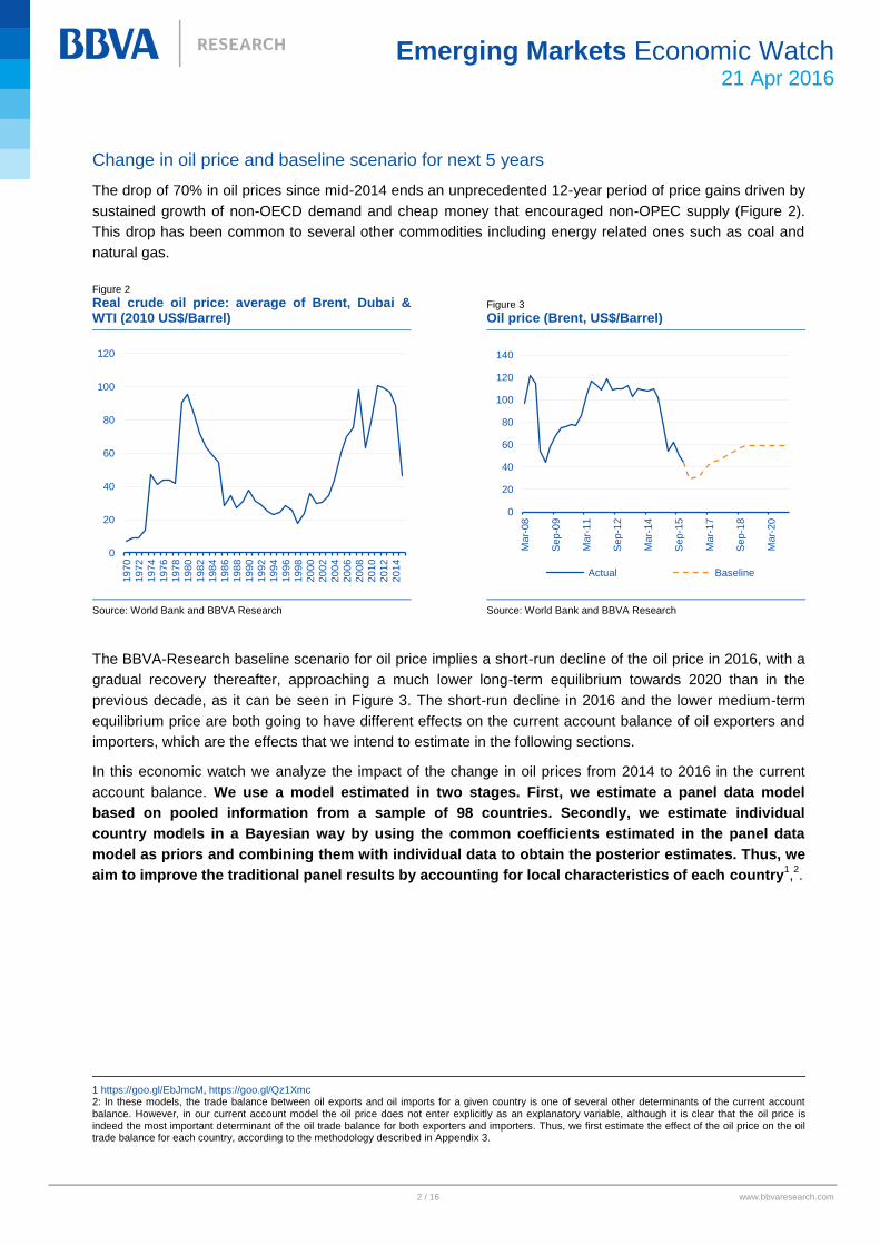
Change in oil price and baseline scenario for next 5 years

The drop of 70% in oil prices since mid-2014 ends an unprecedented 12-year period of price gains driven by

sustained growth of non-OECD demand and cheap money that encouraged non-OPEC supply (Figure 2).

This drop has been common to several other commodities including energy related ones such as coal and

natural gas.

Figure 2

Real crude oil price: average of Brent, Dubai & WTI (2010 US$/Barrel)

Figure 3

Oil price (Brent, US$/Barrel)

Source: World Bank and BBVA Research Source: World Bank and BBVA Research

The BBVA-Research baseline scenario for oil price implies a short-run decline of the oil price in 2016, with a

gradual recovery thereafter, approaching a much lower long-term equilibrium towards 2020 than in the

previous decade, as it can be seen in Figure 3. The short-run decline in 2016 and the lower medium-term

equilibrium price are both going to have different effects on the current account balance of oil exporters and

importers, which are the effects that we intend to estimate in the following sections.

In this economic watch we analyze the impact of the change in oil prices from 2014 to 2016 in the current

account balance. We use a model estimated in two stages. First, we estimate a panel data model

based on pooled information from a sample of 98 countries. Secondly, we estimate individual

country models in a Bayesian way by using the common coefficients estimated in the panel data

model as priors and combining them with individual data to obtain the posterior estimates. Thus, we

aim to improve the traditional panel results by accounting for local characteristics of each country1,2.

1 https://goo.gl/EbJmcM, https://goo.gl/Qz1Xmc 2: In these models, the trade balance between oil exports and oil imports for a given country is one of several other determinants of the current account balance. However, in our current account model the oil price does not enter explicitly as an explanatory variable, although it is clear that the oil price is indeed the most important determinant of the oil trade balance for both exporters and importers. Thus, we first estimate the effect of the oil price on the oil trade balance for each country, according to the methodology described in Appendix 3.

0

20

40

60

80

100

120

19

70

19

72

19

74

19

76

19

78

19

80

19

82

19

84

19

86

19

88

19

90

19

92

19

94

19

96

19

98

20

00

20

02

20

04

20

06

20

08

20

10

20

12

20

14

0

20

40

60

80

100

120

140

Mar-

08

Sep

-09

Mar-

11

Sep

-12

Mar-

14

Sep

-15

Mar-

17

Sep

-18

Mar-

20

Actual Baseline

https://goo.gl/EbJmcM

https://goo.gl/Qz1Xmc



Decomposition of Current Account Balance into Long-term, Medium-term and Cyclical Components

Distinguishing between cyclical and structural current account is important because each component

accounts for a different type of information. On the one hand, the cyclical current account balance is the

component that places a larger pressure on foreign exchange markets and in the short-term financial needs

of a country, increasing/decreasing the likelihood of a currency crisis (large depreciation plus loss of

reserves). On the other hand, the structural balance tells us whether a country will accumulate either foreign

assets or liabilities in a medium- and long-term horizon with a potential impact on its degree of vulnerability.

(The methodology employed to estimate the structural and cyclical current account balances is explained in

Appendix 4).

In order to summarize the results of the exercise, we divide the 98 countries included in the analysis in 9

regional groups (plus the US) according to their geographic and economic relationship. All the results shown

throughout this document are available at a country level upon request. The regions analyzed hereafter are

the following: OPEC and Other Oil Exporters, Emerging Asia, Latam Oil Exporters, Latam Oil Importers,

Africa & MENA, Emerging Europe, Advanced Central Europe, Europe Periphery and non-European

Advanced Economies. The key results of the decomposition of the current account balance into its cyclical

and structural components (Figure 4) are the following:

OPEC and oil exporter’s countries will experience a sharp reduction in their structural surplus of nearly

7% of GDP towards 2020. Currently, they are suffering large adjustments in the cyclical position in

2015 and 2016 (-5% of GDP on average). This will be important as most of these countries have

pegged (or quasi pegged) their currencies with the US dollar. In essence, the ability to maintain these

pegs will diminish.

Oil exporters from Latin America will also experience a deterioration in their structural deficit (from

near zero balance to a structural deficit of -2.4% of GDP in 2020). The rest of Latin America countries

(the net energy importers) will continue to maintain a structural current account deficit that will be

reduced on average by nearly 1% of GDP between 2013 and 2020.

Most of the countries of Emerging Asia will experience a strong trend towards larger structural

surpluses. On average, the structural balance from EM Asia will increase from near 2% in 2013 to

almost 5% of GDP in 2020. As the cyclical position in 2016 will be near 0%, most of the surplus is

structural.

Emerging Europe countries are also among the most benefited and will halve its structural deficit

between 2012 and 2020 (from -3.4 to -1.5% of GDP). As these countries will enjoy a cyclical surplus of

about 0.6% of GDP in 2015 & 2016, their current deficit is mainly structural.

In the case of the Western European countries, we distinguish two groups: The Core Central-European

countries will see an increment in their structural surplus of about 1%. of GDP between 2012 and 2020

(from 1.8 to 2.7) and they will enjoy a cyclical surplus of 0.9 points of GDP this year. The EU Periphery

will be the region with the largest change in its structural balance between 2012 and 2020. It will

go from a structural deficit of -3% of GDP to a structural surplus of 1% of GDP. They will also enjoy

cyclical surpluses of 2.4% and 1.7% of GDP in 2015 and 2016 respectively.

Among the rest of advanced countries, they will only experience a small change in its structural

balance (from 1.6% in 2012 to 1.5% of GDP in 2020). They will nevertheless enjoy a cyclical surplus of

0.8% and 1% of GDP in 2015 and 2016. Surprisingly, the US will not see a large reduction in its

structural deficit and will not even enjoy a cyclical surplus in 2016 (0.5% in 2015 and -0.04% in 2016).



Figure 4

Decomposition of current account balance into structural and cyclical components (% of GDP)

Source: BBVA Research. Note: Notice that years 2017 to 2019 are not depicted in the Graph. The values are weighted averages within each region

The impact of the oil price on the structural & cyclical current account shifts

We have seen that there will be important changes in both the cyclical and structural components of the

current account. In this section we quantify the contribution of the changes in the oil price paradigm to these

changes. In Figure 5 and 6 we can appreciate the contribution of oil price changes to shifts in the structural

(SCAB) and cyclical current account balance together with other economic determinants. We can highlight

the following points:

As expected, the oil balance is the main responsible in the change in the structural CA balance of

OPEC and oil exporters between 2012 and 2020 (an adjustment of nearly 6% of GDP). This will

happen not only through the standard export channel but also through the deterioration in the

fiscal account (nearly -0.8%).

Oil exporters from Latam will suffer a structural drop of about 2% of GDP due to the structural

loss in their oil trade balance. The fiscal balance will contribute with half a point of GDP to the

total loss in their SCAB.

-6

-4

-2

0

2

4

6

8

10

12

20

12

20

13

20

14

20

15

20

16

20

20

20

12

20

13

20

14

20

15

20

16

20

20

20

12

20

13

20

14

20

15

20

16

20

20

20

12

20

13

20

14

20

15

20

16

20

20

20

12

20

13

20

14

20

15

20

16

20

20

OPEC Emerging Asia Latam Oil Exporters Latam Oil Importers Africa & MENA

Structural Cyclical CA/GDP

-5

-4

-3

-2

-1

0

1

2

3

4

20

12

20

13

20

14

20

15

20

16

20

20

20

12

20

13

20

14

20

15

20

16

20

20

20

12

20

13

20

14

20

15

20

16

20

20

20

12

20

13

20

14

20

15

20

16

20

20

20

12

20

13

20

14

20

15

20

16

20

20

Emerging Europe Core Europe Periphery Europe Advanced Economies United States

Structural Cyclical CA/GDP



The most important factor to the Emerging Asia structural balance improvement between 2012

and 2020 will be the medium-term convergence of the region in terms of income per capita and

the reduction of its over-investment levels relative to rest of the World, rather than the oil price.

In Emerging Europe, the change in oil prices will contribute to the reduction in the structural

deficit by about -0.7% of GDP. The cyclical surplus in 2015 and 2016 will come almost entirely from the

effect of the oil balance.

Figure 5

Decomposition of structural current account balance into large economic factors (% of GDP)

Source: BBVA Research. Note: Notice that years 2017 to 2019 are not depicted in the Graph.

-7.5

-5.0

-2.5

0.0

2.5

5.0

7.5

10.0

12.5

20

12

20

13

20

14

20

15

20

16

20

20

20

12

20

13

20

14

20

15

20

16

20

20

20

12

20

13

20

14

20

15

20

16

20

20

20

12

20

13

20

14

20

15

20

16

20

20

20

12

20

13

20

14

20

15

20

16

20

20


Demography Growth&Investment Fiscal balance Financial Factors

Trade & Other factors Oil X-M SCAB

-10

-8

-6

-4

-2

0

2

4

6

8

20

12

20

13

20

14

20

15

20

16

20

20

20

12

20

13

20

14

20

15

20

16

20

20

20

12

20

13

20

14

20

15

20

16

20

20

20

12

20

13

20

14

20

15

20

16

20

20

20

12

20

13

20

14

20

15

20

16

20

20


Demography Growth&Investment Fiscal balance Financial Factors

Trade & Other factors Oil X-M SCAB



Figure 6

Decomposition of cyclical current account balance into large economic factors (% of GDP)

Source: BBVA Research. Note: Notice that years 2017 to 2019 are not depicted in the Graph.

In the advanced European countries the change in its structural balance will be modest, as the

slight improvement in oil will be balanced by demographic factors. The main factor contributing to

the cyclical surplus in 2015 and 2016 is not the oil balance, but the cyclical reduction in private leverage.

In the EU Periphery, the large increase in the structural CA will come from a combination of

several structural factors: the reduction of its energy balance, a reduction of their investment

relative to the rest of the World, the medium-term reduction of its fiscal deficits and the still active

deleveraging process. Although the cyclical effect of the oil price reduction is important (0.7% in 2015

and 0.8% of GDP in 2016), the cyclical effect of the deleveraging process is almost twice as large.

The rest of the Advanced Economies will not experience significant changes in their structural

balances due to different counteracting forces. The structural change in demographic factors

contributes almost the same as the change in the contribution of the oil balance. These countries will

enjoy the largest cyclical effect of the oil price (0.8% and 0.9% of GDP in 2015 and 2016).

In the US, the change in oil prices will not have a large structural effect. The reduction in its fiscal

deficit will have a much larger effect between 2012 and 2020.

-6

-5

-4

-3

-2

-1

0

1

2

3

20

12

20

13

20

14

20

15

20

16

20

20

20

12

20

13

20

14

20

15

20

16

20

20

20

12

20

13

20

14

20

15

20

16

20

20

20

12

20

13

20

14

20

15

20

16

20

20

20

12

20

13

20

14

20

15

20

16

20

20


Fiscal TT & REER Investment & Activity Financial Oil X-M Cyclical

-2.0

-1.5

-1.0

-0.5

0.0

0.5

1.0

1.5

2.0

2.5

3.0

3.5

20

12

20

13

20

14

20

15

20

16

20

20

20

12

20

13

20

14

20

15

20

16

20

20

20

12

20

13

20

14

20

15

20

16

20

20

20

12

20

13

20

14

20

15

20

16

20

20

20

12

20

13

20

14

20

15

20

16

20

20


Fiscal TT & REER Investment & Activity Financial Oil X-M Cyclical



Summing Up: Cyclical and structural winners and losers

The oil price change will have cyclical and structural effects on the current account balances across the

world. There will be winners and losers and among them the positive/negative effects will be felt in an

asymmetric way. First, we are and (will continue to) observe cyclical balance effects exerting pressure on

foreign exchange markets and on the short-term financial needs. In Figures 7a and 7b we can see the

estimated cyclical effect of the oil price change on the cyclical current account balance (through its effect on

the oil trade balance). The main salient features in the cyclical position are the following:

The most benefited countries in terms of cyclical effects this year will be Thailand, Korea,

Singapore, Taiwan, Turkey, Hong Kong, Japan, India and Spain, all of which will enjoy cyclical

contributions of more than 1% of GDP.

In terms of cyclical adjustment the more affected in 2016 are some African countries (Angola,

Nigeria and Algeria), Arabian Peninsula countries (Kuwait, Saudi Arabia, Oman, UAE, Qatar and

Bahrain), Azerbaijan and Russia in Emerging Europe, and Venezuela, Ecuador, Colombia and

Mexico in Latin America. Some traditional oil exporters such as Libya and Iran are somewhat less

affected because they were exporting much less oil than usual before 2015.

On average, the cyclical effect of the oil balance on the CA balance is -2.7% of GDP for traditional

oil exporters, and 0.9% of GDP for traditional oil importers.

Similarly, there will be winners and losers in terms of changes in the structural CA balance due to the

long-term reduction in the oil price (lower equilibrium price in 2020).This will affect the accumulation of

foreign assets/liabilities in the future due to the permanent change in the oil trade balance. This should have

more permanent effects thus altering some of the equilibrium exchange rates.

In Figures 8a and 8b we can observe the change in the SCAB that is due to the change in the oil price in the

medium-term. The graphs display the change in the contribution of the oil trade balance to the SCAB in

2020 compared to the SCAB in 2012. From this difference we can point out the following key points:

Oil exporters evidently top the structurally damaged countries’ list. Some countries such as Azerbaijan,

Angola or Nigeria will suffer sharp structural adjustments, moving from being strong accumulators of

foreign assets thanks to their oil trade balances, to net accumulators of foreign liabilities. The strong

export position of Persian Gulf countries (Qatar, Saudi Arabia, Oman, etc.) during the past will

prevent these countries from becoming net dissavers, but the rate at which they accumulate

foreign assets thanks to their oil exports will be largely reduced.

On the opposite side, several countries such as Lebanon, Korea or Taiwan will almost reduce their

structural external financial needs from oil trade to almost 0% of GDP. Other countries such as

Thailand, Morocco or Turkey will reduce their structural financial needs (from their trade in oil) by

more than half their structural needs in 2012.



Figure 7a

Cyclical losers from the oil price decline (Cyclical effect on the CAB in % of GDP)

Figure 7b

Cyclical winners from the oil price decline (Cyclical effect on the CAB in % of GDP)


Figure 8a

Structural losers from the oil price decline (Structural change between 2012-2020 in % of GDP)

Figure 8b

Structural winners from the oil price decline (Structural change between 2012-2020 in % of GDP)


In Appendix 2 we show the complete lists of countries according to the estimated effects of the oil price

change on the cyclical (Table 1) and structural (Table 2) current account balances.

-10 -8 -6 -4 -2 0

Angola

Azerbaijan

Kuwait

Saudi Arabia

Oman

UAE

Nigeria

Algeria

Venezuela

Qatar

Bahrain

Russia

Ecuador

Colombia

Trin. & Tob.

0 1 2 3 4

Spain

India

Portugal

Japan

Bulgaria

Hong Kong

Turkey

Namibia

Taiwan

Singapore

Korea

Jamaica

Morocco

Thailand

Nicaragua

-20 -15 -10 -5 0

Azerbaijan

Angola

Qatar

Algeria

Saudi Arabia

Nigeria

Oman

UAE

Kuwait

Mexico

Belarus

Iran

Norway

Malaysia

Libya

Ecuador

Russia

0 1 2 3 4

Turkey

Philippines

Bulgaria

Singapore

Paraguay

El Salvador

Taiwan

Bosnia & Herz.

Hong Kong

Lithuania

Korea

Morocco

Thailand

Nicaragua

Honduras



Appendix 1

List of countries included within each region

The values for each group shown throughout this document represent a weighted average within each

region, with the weights given by the share of each country’s GDP on the total group GDP (in PPP US$).

OPEC and Other Oil Exporters: Algeria, Angola, Azerbaijan, Bahrain, Iran, Kuwait, Libya, Nigeria,

Norway, Oman, Qatar, Russia, Saudi Arabia and United Arab Emirates

Emerging Asia: Bangladesh, China, Hong Kong, India, Indonesia, Malaysia, Myanmar, Pakistan,

Philippines, Sri Lanka, Taiwan, Thailand and Vietnam.

Latam Oil Exporters: Colombia, Ecuador, Mexico, Trinidad & Tobago and Venezuela.

Latam Oil Importers: Argentina, Bolivia, Brazil, Chile, Costa Rica, Dominican Rep., El Salvador,

Guatemala, Honduras, Jamaica, Nicaragua, Panama ,Paraguay, Peru and Uruguay.

Africa & MENA: Botswana, Cameroon, Egypt, Israel, Lebanon, Morocco, Namibia, South Africa and

Tunisia

Emerging Europe: Armenia, Belarus, Bosnia and Herzegovina, Bulgaria, Croatia, Cyprus, Czech

Republic, Estonia, Hungary, Latvia, Lithuania, Poland, Romania, Slovak Rep, Slovenia, Turkey, Ukraine

Core Europe: Austria, Belgium, Denmark, Finland, France, Germany, Luxembourg, Netherlands,

Sweden and United Kingdom.

Periphery Europe: Greece, Ireland, Italy, Malta, Portugal and Spain

Advanced Economies: Australia, Japan, Korea, Singapore, Canada, Iceland, New Zealand and

Switzerland.



Appendix 2

List of countries according to the impact of the oil price change

Table 1

Short-term contribution of oil balance to the cyclical current account in 2016 (% of GDP)

Harmed countries Mildly benefited countries Highly benefited countries

1 Angola -11.5 31 UK 0.0 69 Pakistan 1.0

2 Azerbaijan -9.9 32 Bangladesh 0.0 70 Luxembourg 1.0

3 Kuwait -7.7 33 Romania 0.0 71 Guatemala 1.0

4 Saudi Arabia -6.8 34 Slovak Rep 0.1 72 Spain 1.0

5 Oman -6.3 35 Denmark 0.1 73 India 1.0

6 UAE -5.1 36 Indonesia 0.2 74 Portugal 1.0

7 Nigeria -3.8 37 Australia 0.3 75 Cyprus 1.0

8 Algeria -3.7 38 Myanmar 0.3 76 Japan 1.0

9 Venezuela -3.6 39 France 0.3 77 Sri Lanka 1.0

10 Qatar -3.1 40 Brazil 0.3 78 Bulgaria 1.0

11 Bahrain -3.0 41 Chile 0.4 79 Latvia 1.1

12 Russia -2.2 42 Armenia 0.4 80 Paraguay 1.1

13 Ecuador -1.4 43 Netherlands 0.4 81 Iceland 1.2

14 Colombia -1.3 44 Estonia 0.4 82 Hong Kong 1.3

15 Trin. & Tob. -1.3 45 USA 0.4 83 Turkey 1.3

16 Mexico -1.1 46 Sweden 0.5 84 El Salvador 1.4

17 Norway -1.1 47 South Africa 0.5 85 Namibia 1.5

18 Libya -0.9 48 New Zealand 0.5 86 Taiwan 1.6

19 Cameroon -0.9 49 Finland 0.5 87 Bosnia & Herz. 1.7

20 Malaysia -0.9 50 Bolivia 0.6 88 Singapore 1.7

21 Canada -0.6 51 Switzerland 0.6 89 Lithuania 1.8

22 VietNam -0.6 52 Israel 0.6 90 Malta 1.9

23 Belarus -0.4 53 Italy 0.6 91 Honduras 2.0

24 Ukraine -0.2 54 China 0.6 92 Korea 2.1

25 Peru -0.2 55 Germany 0.7 93 Jamaica 2.4

26 Croatia -0.1 56 Ireland 0.7 94 Botswana 2.6

27 Egypt 0.0 57 Austria 0.7 95 Morocco 2.7

28 Iran 0.0 58 Belgium 0.7 96 Thailand 2.9

29 Tunisia 0.0 59 Panama 0.7 97 Lebanon 3.0

30 Argentina 0.0 60 Uruguay 0.7 98 Nicaragua 3.0

61 Dominican Rep 0.8

62 Philippines 0.8

63 Czech Rep. 0.8

64 Slovenia 0.8

65 Costa Rica 0.9

66 Poland 0.9

67 Hungary 0.9

68 Greece 0.9

Source: BBVA Research



Table 2

Loss/Gain in structural current account balance in 2020 vs. 2012 due to the lower oil balance (% of GDP)

Harmed countries Mildly benefited countries Highly benefited countries

1 Azerbaijan -27.3 34 Slovenia 0.0 67 Latvia 0.7

2 Angola -17.1 35 UK 0.0 68 Costa Rica 0.8

3 Qatar -16.9 36 Chile 0.0 69 Hungary 0.8

4 Algeria -10.2 37 Ukraine 0.0 70 China 0.8

5 Saudi Arabia -8.6 38 Bangladesh 0.1 71 Dominican Rep 0.8

6 Nigeria -6.9 39 Slovak Rep 0.1 72 Sri Lanka 0.8

7 Oman -3.6 40 New Zealand 0.1 73 Poland 0.9

8 UAE -2.5 41 Brazil 0.1 74 Guatemala 0.9

9 Kuwait -2.4 42 Australia 0.2 75 Pakistan 0.9

10 Mexico -2.2 43 Croatia 0.2 76 Uruguay 0.9

11 Belarus -1.8 44 Portugal 0.2 77 Turkey 1.0

12 Iran -1.5 45 France 0.2 78 Iceland 1.0

13 Tunisia -1.5 46 Czech Republic 0.3 79 Luxembourg 1.0

14 Norway -1.4 47 VietNam 0.3 80 Philippines 1.1

15 Malaysia -1.4 48 Panama 0.4 81 Bulgaria 1.2

16 Libya -1.3 49 Belgium 0.4 82 Singapore 1.2

17 Ecuador -0.9 50 Cyprus 0.4 83 Paraguay 1.5

18 Russia -0.8 51 Netherlands 0.4 84 Malta 1.7

19 Bahrain -0.8 52 South Africa 0.4 85 El Salvador 1.7

20 Colombia -0.7 53 India 0.4 86 Taiwan 1.7

21 Indonesia -0.6 54 Germany 0.5 87 Bosnia & Herz. 1.7

22 Estonia -0.6 55 Spain 0.5 88 Hong Kong 1.8

23 Argentina -0.6 56 Bolivia 0.5 89 Lithuania 2.1

24 Cameroon -0.6 57 Israel 0.6 90 Korea 2.1

25 Armenia -0.5 58 Sweden 0.6 91 Morocco 2.3

26 Romania -0.3 59 Finland 0.6 92 Thailand 2.4

27 Denmark -0.3 60 Austria 0.6 93 Namibia 2.4

28 Canada -0.3 61 Greece 0.6 94 Nicaragua 2.5

29 Egypt -0.2 62 Switzerland 0.7 95 Botswana 2.6

30 Venezuela -0.2 63 Japan 0.7 96 Honduras 3.1

31 Myanmar -0.1 64 Italy 0.7 97 Jamaica 3.1

32 Peru -0.1 65 United States 0.7 98 Lebanon 3.5

33 Trin. & Tob. -0.1 66 Ireland 0.7

Source: BBVA Research



Appendix 3

Estimation of the effect of the oil price on the oil trade balance

The oil trade balance of a country is defined as the difference between the value of oil exports and of oil

imports as a percentage of its GDP. The oil trade balance depends on the volume of oil produced by each

country, on its own internal demand, and on the international and the local prices of oil. However, we do not

have information on the amount produced or demanded by every country for such a large group of countries

as the one analyzed here. Therefore, we have to assume that most of this information is captured by each

country’s own sensitivity to the price of oil.

Due to different reasons we estimate four different types of models to form a final forecast. All four models

include the same explanatory variables, but they differ on whether they are expressed in levels or in

changes, and on whether the model is estimated individually for each country or in a pooled sample. The

dependent variable is the oil balance (%GDP) and the explanatory variables are: i) the lagged oil trade

balance; ii) the real price of oil; and iii) the relative real income per capita. The relative income per capita is

calculated as each country’s deviation from the World’s average income. GDP per capita is measured in

PPP terms, and in real US dollars.

Our final prediction for the oil balance comprises a weighted average of the four predictions coming from the

four different models. The weight that is assigned to each model’s prediction is estimated as the inverse of a

mean square error of prediction. The error of prediction is estimated as the difference between the

prediction made by each model for the year 2016 and the actual oil balance value in the year 2002, which

corresponds to the year in which the oil price was closer to its expected value in 2016. We also estimate a

similar error of prediction for the difference between the years 2020 vs. 2005.

The first model is a simple regression for each one of the 98 countries of the sample. However, since some

countries have a very short data history, we also estimate a panel data regression. But since we do not

have information on the volume produced or consumed by each country, we separate all countries into four

different groups according to their historical oil balance average, and we estimate four different panel

regressions, one for each group.

In Figures 9 and 10 we show a couple of examples of how we obtain our final prediction for the oil trade

balance from the four different model specifications that are estimated for each country. In the graphs we

can observe the actual oil trade balance for two different countries (one exporter and one importer), which is

denoted as “Final”. The actual observed data goes up until 2014 or 2015 in most cases (in some cases we

only have data up until 2012). Afterwards we can observe the different paths predicted by each one of the

four alternative models and the “final” weighted average of the predictions.



Figure 9

Oil trade balance (%GDP) Spain: Actual, different forecasts and final forecast

Figure 10

Oil trade balance (%GDP) Saudi Arabia: Actual, different forecasts and final forecast

Source: BBVA Research Source: BBVA Research

-5.0

-4.5

-4.0

-3.5

-3.0

-2.5

-2.0

-1.5

-1.0

-0.5

0.0

19

86

19

88

19

90

19

92

19

94

19

96

19

98

20

00

20

02

20

04

20

06

20

08

20

10

20

12

20

14

20

16

20

18

20

20

Individual (changes) Panel (changes)

Individual (levels) Panel (levels)

Final

0

10

20

30

40

50

60

19

86

19

88

19

90

19

92

19

94

19

96

19

98

20

00

20

02

20

04

20

06

20

08

20

10

20

12

20

14

20

16

20

18

20

20

Individual (changes) Panel (changes)

Individual (levels) Panel (levels)

Final



Appendix 4

Modeling and decomposing the current account balance

The methodology used for estimating the structural and cyclical current account balance and its

determinants is fully explained in the Economic Watch “An analysis of the performance and the determinants

of the current account in Spain” that can be found here: https://goo.gl/EbJmcM.

In our Current Account Model, each explanatory variable is broken-down into three components depending

on their frequency of oscillation, i.e. long-term, medium-term and short-term, and further, we allow each of

them has its own estimated effect on the observed current account to GDP ratio. The estimated model is,

thus, as follows:

𝐶𝐶𝑖𝑡 = �̅�𝑖′𝛽𝐿𝑇 + (�̅�𝑖𝑡𝑀𝐴5𝑦

− �̅�𝑖)′𝛽𝑀𝑇 + (𝑋𝑖𝑡 − �̅�𝑖𝑡𝑀𝐴5𝑦

)′𝛽𝑆𝑇 + 𝑍𝑖𝑡′𝜑𝐶𝑌𝐶 + 𝛿𝑖 + 𝑢𝑖𝑡, (1)

where 𝐶𝐶𝑖𝑡 is the actual current account to GDP ratio; �̅�𝑖 includes the long-term average of each explanatory

variable (measured according to the historical average of each country) and 𝛽𝐿𝑇 is the long-term coefficient

vector associated with these averages; (�̅�𝑖𝑡𝑀𝐴5𝑦

− �̅�𝑖) represents the medium-term deviation of the

explanatory variables vs their long-term values (5Y moving average vs. average over time by country) and

𝛽𝑀𝑇 is the medium-term coefficient vector; (𝑋𝑖𝑡 − �̅�𝑖𝑡𝑀𝐴5𝑦

) represents the deviation of the observed

explanatory variables vs their medium-term average (actual value vs. 5Y moving average) and 𝛽𝑆𝑇 is the

short-term coefficient vector; 𝑍𝑖𝑡 is a vector of purely cyclical explanatory variables and 𝜑𝐶𝑌𝐶 is the

corresponding coefficient vector.

Through this model we are not only able to decompose the current account ratio of each country into its

structural and cyclical component, but we are also able to decompose each component into their own

determinants, which are given by the long- and medium-term effects of the explanatory variables for the

structural component, and the short-term effects in the case of the cyclical component.

Thus, we are able to estimate the contribution of the oil trade balance to the present and future current

account balance and decompose it into its structural and cyclical contributions.

One of the main advantages of our methodological strategy is that although the cyclical and structural

components of any variable could be estimated through some often used filters such as the Hodrick-Prescott

filter, we are also able to further break-down the estimated components into their economic determinants,

something that is not possible with the alternative methodologies.

Through this methodology, the fitted value of the structural current account is obtained using the long- and

medium-term components of the explanatory variables and their corresponding estimated effect.

The model is estimated in a panel data of 92 countries for the period 1980-2014 containing 1,973

observations. The database is constructed using IMF-WEO, World Bank, UN, OECD, Darvas (2012) and

BBVA Research data. All the variables are expressed in terms of deviations from its respective global

average, except for the dependent variable, the initial NIIP, the oil trade balance and variations in the

exchange rate, as in these cases the global average would be zero. The estimation is made using feasible

generalised least squares (FGLS) and the variance-covariance matrix is adjusted to correct for

heteroskedasticity and autocorrelation of residuals.

Subsequently, the estimation of the short- and medium-term coefficients resulting from the panel data

approach is adapted to the each one of the 92 countries. Specifically, these coefficients are re-estimated

using a Bayesian time-series model designed for each country. In particular, the Bayesian model uses the

short- and medium-term coefficients obtained from the panel data model, as well as their distribution, as

https://goo.gl/EbJmcM



priors for the Bayesian estimation. The long-term coefficients estimated through the panel data model remain

unchanged.

Table 3 shows that most of the results obtained from the panel data model are in line with the economic

literature, albeit the methodology used in this report allows a different response of each variable in the long

and medium-term (structural effect) and the short-term (cyclical effect).

Table 3

Current account models: Panel data model estimation results

Explanatory variables

Panel Data Model Estimation

Long-term Mid-term Short-term

Old dependency ratio (population older than 65 years old as % of population between 15- 64 years old)

-0.12** -0.23***

Population Growth (%) 0.81** -0.52***

Public Health Expenditure (%GDP) -0.84*** -0.53***

Investment (%GDP) -0.12** -0.54*** -0.61***

GDP per cppita (log USD ajustados-PPA) 3.55***

Fiscal Balance (%GDP) 0.257*** 0.295*** 0.117***

Private Credit (%GDP) 0.038*** -0.02*** -0.066***

Initial NIIP (%GDP) 0.024*** 0.001 0.010**

Short-term interest rate -0.029* 0.002

Trade openness (exports and imports as % of GDP) 0.034*** 0.035*** 0.014*

Oil balance (%GDP) 0.220*** 0.645*** 0.707***

Output gap (difference between observed and potential GDP as % of potential GDP)

-0.067***

Terms of trade (% change) 0.013***

Terms of trade (% chante in t-1) 0.012***

Real effective exchange rate -0.018***

Interest rate in USA (%) 0.100***

VIX (% change) 0,012**

Observations: 1973

R-squared = 0,82

Notes: ***, **, * denote statistical significance at 1%, 5% and 10% levels, respectively. The estimations include only a cyclical effect of the last six explanatory variables. The panel data model is estimated through FGLS. In the Bayesian estimation it is assumed that the long-term coefficients estimated in the panel data model remain unchanged. Source: BBVA Research



DISCLAIMER

This document has been prepared by BBVA Research Department, it is provided for information purposes only and

expresses data, opinions or estimations regarding the date of issue of the report, prepared by BBVA or obtained from or

based on sources we consider to be reliable, and have not been independently verified by BBVA. Therefore, BBVA offers

no warranty, either express or implicit, regarding its accuracy, integrity or correctness.

Estimations this document may contain have been undertaken according to generally accepted methodologies and

should be considered as forecasts or projections. Results obtained in the past, either positive or negative, are no

guarantee of future performance.

This document and its contents are subject to changes without prior notice depending on variables such as the economic

context or market fluctuations. BBVA is not responsible for updating these contents or for giving notice of such changes.

BBVA accepts no liability for any loss, direct or indirect, that may result from the use of this document or its contents.

This document and its contents do not constitute an offer, invitation or solicitation to purchase, divest or enter into any

interest in financial assets or instruments. Neither shall this document nor its contents form the basis of any contract,

commitment or decision of any kind.

In regard to investment in financial assets related to economic variables this document may cover, readers should be

aware that under no circumstances should they base their investment decisions in the information contained in this

document. Those persons or entities offering investment products to these potential investors are legally required to

provide the information needed for them to take an appropriate investment decision.

The content of this document is protected by intellectual property laws. It is forbidden its reproduction, transformation,

distribution, public communication, making available, extraction, reuse, forwarding or use of any nature by any means or

process, except in cases where it is legally permitted or expressly authorized by BBVA.

The current account balance and the oil price shock

Documents

Transcript of The current account balance and the oil price shock