The crippled queen placement problem
28
Science of Computer Programming 4 (1984) 221-248 North-Holland 221 THE CRIPPLED QUEEN PLACEMENT PROBLEM Robert WAGNER and Robert GEIST* Department of Computer Science, Duke University, Durham, NC 27706, U.S.A. Communicated by R. Sethi Received October 1983 Revised January 1984 Abstract. We describe the outcome of various combinations of choices made by individuals in the solution of a non-trivial combinatorial problem on a computer. The programs which result are analyzed with respect to execution speed, design time, and difficulty in debugging. The solutions obtained vary dramatically as a result of choices made in the overall design of the solution. Choices made at lower levels in the top-down tree of design choices seem to have less effect on the parameters analyzed. A tradeoff between mathematical effort in algorithm design, and program speed is evident, since some solutions required solution-time which grows exponentially with the case size, while another solution presented here gives a closed-form expression for the required answers for all large cases. Introduction This paper is an attempt to document the major choices made in designing a computer program to solve a non-trivial problem, a variation of the classical eight queens problem [ 1,3], originally posed by Franz Nauck in 1850. Like the eight queens problem, it is representative of a large class of combinatorial problems and is mathematically interesting in its own right. We hope that it is also representative of problems encountered by programmers in practice. In presenting solutions, we attempt to exhibit tradeoffs between two principal categories of variables: (1) The effort expended in mathematical analysis of the problem, before code (or even coding specification) is developed, and (2) The ‘quality’ of the resulting program product, measured in terms of (a) execution speed, (b) textual compactness and clarity, (c) difficulty in debugging (more generally, difficulty in obtaining acceptably high confidence in program correctness). We observe that choices made at high levels of abstraction have much larger impact on quality and involve a much higher level of analytic effort than choices * Current address: Department of Computer Science, Clemson University, Clemson, SC 2963 I, U.S.A. Ol67-6423/84/%3.00 @ 1984, Elsevier Science Publishers B.V. (North-Holland)
-
Upload
robert-wagner -
Category
Documents
-
view
214 -
download
1
Transcript of The crippled queen placement problem
Science of Computer Programming 4 (1984) 221-248
North-Holland
221
THE CRIPPLED QUEEN PLACEMENT PROBLEM
Robert WAGNER and Robert GEIST*
Department of Computer Science, Duke University, Durham, NC 27706, U.S.A.
Communicated by R. Sethi
Received October 1983
Revised January 1984
Abstract. We describe the outcome of various combinations of choices made by individuals in
the solution of a non-trivial combinatorial problem on a computer. The programs which result
are analyzed with respect to execution speed, design time, and difficulty in debugging. The solutions
obtained vary dramatically as a result of choices made in the overall design of the solution.
Choices made at lower levels in the top-down tree of design choices seem to have less effect on
the parameters analyzed. A tradeoff between mathematical effort in algorithm design, and program
speed is evident, since some solutions required solution-time which grows exponentially with the
case size, while another solution presented here gives a closed-form expression for the required
answers for all large cases.
Introduction
This paper is an attempt to document the major choices made in designing a
computer program to solve a non-trivial problem, a variation of the classical eight
queens problem [ 1,3], originally posed by Franz Nauck in 1850. Like the eight
queens problem, it is representative of a large class of combinatorial problems and
is mathematically interesting in its own right. We hope that it is also representative
of problems encountered by programmers in practice.
In presenting solutions, we attempt to exhibit tradeoffs between two principal
categories of variables:
(1) The effort expended in mathematical analysis of the problem, before code
(or even coding specification) is developed, and
(2) The ‘quality’ of the resulting program product, measured in terms of
(a) execution speed,
(b) textual compactness and clarity,
(c) difficulty in debugging (more generally, difficulty in obtaining acceptably
high confidence in program correctness).
We observe that choices made at high levels of abstraction have much larger
impact on quality and involve a much higher level of analytic effort than choices
* Current address: Department of Computer Science, Clemson University, Clemson, SC 2963 I, U.S.A.
Ol67-6423/84/%3.00 @ 1984, Elsevier Science Publishers B.V. (North-Holland)
222 R. Wagner, R. Geisf
made to solve ‘subproblems’. In particular, we observe large improvements in
execution speed as a result of additional analytic effort. This is accompanied by
little or no change in measures of textual acceptability, and/or debugging difficulty.
In contrast, one subproblem, generated to help implement one solution technique,
required large inputs of analytic effort, but generated a large percentage of the
program text and the debugging difficulties observed. Moreover, solving this sub-
problem probably contributed a comparatively small speed improvement.
We conclude by suggesting that, in the hierarchical development of a program,
whenever possible, one should attempt to judge execution speed and conceptual
difficulty of implementing a (sub) program, before proceeding to the next stage of
hierarchical refinement. At the moment, some analytic tools for estimating worst-case
run-time are available; however, no simple, trustworthy methods for average run-
time estimation are known, primarily because the probability of occurrence of any
identifiable subclass of problem instances is unknown. Also, we know of no quantita-
tive method of estimating, in advance, measures of program complexity, under-
standability, and debuggability. Thus, our planning is haphazard and subject to
error in these areas. By studying the program development process, we hope to shed
some light on the choices made during program development that control the
performance, complexity, and size of implementation of the resulting product.
The remainder of the paper is organized as follows. The problem and its straightfor-
ward solution are presented in Section 1. The straightforward solution is readily
seen to be unacceptable, and so a necessary improvement is also presented there.
In Section 2, a deeper analysis of the problem is combined with the technique of
Dynamic Programming [2,4] to yield first a modest success and then a substantial
improvement thereon. In Section 3, geometric reduction and mathematical induction
are applied to obtain a closed form solution for most problem instances. Comparisons
and conclusions are presented in Sections 4 and 5 respectively.
1. The problem
The following problem was presented to a class of graduate students in Computer
Science. It was chosen by one of the authors (Wagner) as a natural generalization
of the familiar S-queens problem [l]. The problem was chosen to be ‘non-trivial’,
in that it was hoped that many programs using distinctly different strategies could
be invented for its solution.
“A Crippled Queen (CQ) is a chess queen that can move at most 2 squares at a
time in any queen-attack direction (vertical, horizontal, or diagonal). Find the
number C,, of such CQ’s that can be placed on an 8 ~8 chess board so that no two
attack one another. Find also Nss, the number of different ways C,, CQ’s can be
so placed. If possible, generalize the program to compute C,, and N,,, or C,,,. and
N,,,,, defined as above, but for an 8 x n or m x n chessboard. Your program’s run
time will be one criterion for determining its grade.”

The crippled queen placemenr problem 223
1.1. Its straightforward solution
Most of the class wrote straightforward generalizations of the simplest g-queens
solution. In this backtracking approach, a recursive routine searches over a linear
ordering of the m*n squares for the next unattacked square, marks that square
occupied, marks appropriate adjacent squares attacked, and calls itself to proceed
with the search from that point. When the board is full, the routine recursively
removes the last-placed CQ and seeks the next possible location for it in the linear
ordering. We present this and all other programs in a ‘pidgin’ version of C [5]:
Solution 1. global integer BOARD[M * NJ, /* indicates which squares are currently
occupied, and/or attached. */
main ( ) {
Cmn = 0; /* maximum number of CQ’s placed */
Nmn = 1; /* number of solutions with Cmn CQ’s */
place( I ) ;
1
pldsq) integer sq;{
local integer s ;
s=sq;
while(s G m *n){
if (BOARD[S] is unattacked by previously placed CQ’s)
{Mark BOARD[S] occupied;
place( nextsq[s]);
Mark BOARD[S] unoccupied;}
s = nextsq[s];
/* Board is full */
C= # squares marked occupied;
if (C>Cmn) {Cmn=C; Nmn= 1);
if (C= =Cmn) Nmn=Nmn+l;
return: /* from place() */
Here nextsq[s] gives the square numbered next after s in the linear ordering of
the m * n squares.
1.2. A necessary improvement
Unfortunately, while Solution 1 satisfies the originally-stated specifications, it is
not acceptable: its execution for the 8 ~8 case uses from 40 to 240 minutes of
PDP-I I /70 time.

221 R. Wagner. R. Geist
Experiments showed that execution time could be dramatically improved by
refusing to extend a partial solution that placed, say, k CQ’s in the first x columns
of the board if k + Cm,n-.x, < C,,, where, as before, C,,,, denotes the maximum
number of CQ’s placeable on an m row by j column board.
Execution times for solutions incorporatin g this ‘branch-and-bound’ strategy
ranged from 4.8 to 35.7 seconds on the PDP-1 l/70, for the 8 x8 case. A typical
version, incorporating the suggested modification is:
Solution 2.
global integer BoARD[m * n], Cmn, Nmn, Cm[n + 11;
global integer j; /* columns in current board */
global integer k: /* CQ’s placed in first x cols of current board */
main( ) {
for (j= 1; jSn; j=j+l){
k=O;
Cmn = 0;
Nmn = 1.;
place( 1) ;
Cm[ j] = Cmn ;
I /*There are ‘Nmn’ solutions which place ‘Cmn’ CQ’s on the ‘m by
‘n’ chessboard */}
place(sq) integer sq;{
local integer s;
s=sq;
while( s s m *j){
if (k +Cm[j - column[s]] < Cmn) break;
if (BOARD[S] is unattacked by previously placed CQ’s)
{Mark BOARD[S] occupied;
k=k+l;
place(nextsq[s]);
k=k-1:
Mark BOARD[S] unoccupied:]
s = nextsq[s];
1 /* m by j board is full */
if (k>Cmn) {Cmn=k; Nmn=l:}
if (k= =Cmn) Nmn=Nmn+l;
return;
]

The crippled queen placement problem 225
Here, column[s] gives the column number (from 1 to n) of the column in which
square s occurs. Both nextsq and column are arrays, which can be initialized before
the main computation begins.
The fastest versions of this strategy caused the “Mark BOARD[S] occupied” step
to also mark all squares t such that t > s, and a CQ on square s attacks square t as
‘attacked (again)‘, usually by incrementing an ‘attack count’ associated with each
such square. To simplify the edge-of-board problems, the array BOARD was often
augmented to an (m +4) by (n +4) array, allowing the ‘real’ board to be bordered
by two rows and two columns of ‘off-board’ squares on each side. Slower versions
of the program failed to include the loop to calculate Cm[j], but instead relied on
(a) a formula, such as Cm[j] < 3j (for the M = 8 case)-no more than 3 CQ’s can
be placed in one column without mutual attacks; or
(b) re-running the program by hand for several successive values of n, and filling
in the Cm[ ] table using the results of those runs manually.
A plot of the time needed to solve the 8 x n case showed that all programs using
this strategy ran in exponential time as a function of n. In fact, under a IO-minute
CPU time limit, the case 8 x 16 proved to be out of reach for even the fastest program.
2. A deeper analysis?
Is it possible to further improve the speed-of-solution of an algorithm for the CQ
problem?
Readers interested in problem-solving techniques are urged at this point to answer
this question for themselves, before reading further sections. They may assume that
solutions for large values of m, or of n, or of m * n are needed for some reason,
and that run time for these generalized problems are to be limited to no more than
10 minutes of CPU time on a PDP- 1 l/70.
2.1. A deeper analysis
Dynamic Programming [2,4] can sometimes be applied to combinatorial problems
to yield significant gains in speed-of-solution. Unfortunately, it is often difficult to
see how to apply it, even when the technique is familiar to the analyst/programmer.
In the present case, considerable thought was expended on several blind alleys
before achieving some modest success:
Blind alley 1. Consider solving the CQ problem on an (n + 1) by (n + 1) board,
given some (constrained) solution-information for the i x i boards, id n. This approach proved unpromising, since it appeared that
(a) there were a large number of ways of bordering an n x n board with patterns
of non-attacking CQ’s in a border row-and-column;
226 R. Wagner, R. Geisr
(b) the constraints imposed by each such border pattern amounted to deleting certain ragged patterns of edge squares from the n x n board; initial analysis seemed to show that some 4” different ‘ragged boards’ of maximum dimension n x n might have to be considered.
Blind alley 2. Try increasing the size of a board by one square, instead of bordering an n x n board with an entire row-and-column of CQ’s. This approach seemed worse than # 1, and was quickly (perhaps too quickly?) abandoned.
2.2. Modest success
Try solving the m x n board in terms of constrained solutions to the m x (n - 1)
board. The most important conceptual milestones in the development of this solution were:
(1) an experimental determination (Anselmo Lastra), that there were only 28 different non-attacking CQ placement patterns on the 8 x 1 board;
(2) a realization that the ‘constraints’ needed on the m x (n - 1) board could be described compactly by fixing the CQ patterns present in the last two columns of the m X (n - 1) board. The ‘legality’ of a specific pattern occurring in the nth column can then be determined.
The following reformulation of the CQ problem resulted (we number columns from right to left for this formulation): Fix m and let Cm(S, T, i) be the maximum number of CQ’s placeable on an m row by i column board whose last and next to last columns hold CQ patterns ‘9 and ‘T’ respectively, where iz2. If we let XII Y (Xl Y) denote the binary relation on pattern numbers which is true if and only if pattern number X can be placed 2 columns (1 column) away from pattern number Y without CQ attacks resulting, then for i> 2, we have Cm( R, S, i) = max,{IRI+Cm(S, T, i-1):SlT and R/IT}, if RIS, and 0 otherwise, where jRI= number of CQ’s in pattern number R. Clearly Cm(R, S, 2) = IRI +ISI, if RIS, and 0 otherwise, and max,,,, {Cm( R, S, n) : RIS} is the maximum number of CQ’s place- able on the m x n board.
Furthermore, if we define Nm( R, S, i) = number of solutions to the CQ placement problem on the m X i board containing Cm( R, S, i) CQ’s, where the last two columns of the board hold patterns numbered R and S, respectively, then Nm(R, S. i) can then be computed as follows:
Nm(R, s, 2) = 1 if RIS,
o otherwise
1
and for i > 2,
T {Nm(S, T, i- 1): SIT, RIIT
Nm( R, S, i) = and IRI+Cm(S, T, i- 1) =Cm(R, S, i)} if RIS,
0 otherwise.
7he crippled queen placemenr problem 227
The reader should find it easy to verify that, if an m x i board (i > 2) holds a
maximal number of non-attacking CQ’s, and its last two columns hold patterns R and S respectively, then some pattern T occupies column i - 2 such that: RIS and
Sl T and R 11 T and columns 1 to i - 1 contain Cm(S, T, i - 1) CQ’s. (For they could
never contain more than this number of CQ’s, since Cm( S, T, i - 1) is the maximum
number of CQ’s so placeable by definition; while if they contained fewer CQ’s, the
value of Cm(R, S, i) could be increased, contradicting its definition.)
We have thus established
Solution 3. for (i=2; isn; i=i+l){
for (all (R, S) such that (RIS)) { use above relations to tabulate Cm[R, S, i] and Nm[R, S, i]
1
1 Cmn=O;
Nmn=O;
for (all R, S) such that (RIS)) { C = Cm[R, S, n];
if (C> Cmn) {Cmn = C; Nmn = 0;)
if (C = = Cmn) Nmn = Nmn + Nm[R, S, n];
1
For fixed m, let P,,, be the set of legal patterns for the m x I board, that is, the set of
solutions to the problem of placing any number of CQ’s on the m x 1 board without
mutual attacks. Then assuming that X( Y and XI] Y have been pre-tabulated for all
X, YE P,,,, solution 3 requires running time 0( pin), where pm = ]P,,,/. Since ps z 28,
this gives an 0(283 n) run-time for the 8* n case of the CQ problem. In general, the
run-time for this solution is linear in n. We estimate that about 20 psec would be used
per iteraton of the inner loop, giving a ‘slope’ of about 20 x 22000 x 10m6 = 0.44 seconds
per column. In 10 minutes, or 600 seconds, the case 8 x 1300 could be solved, using
space for about 1300 x28 x 28 = 1 020 000 integers. (In practice, since only the tables
for i and i - 1 need be present when computing the Cm[ ] and Nm[ ] tables for i, required
storage is independent of n.)
This scheme is somewhat limited, however, since pm s 2m’3. This can easily be
seen as follows. pm gives the number of placements of CQ’s possible in one column
of m squares without mutual attacks. But CQ’s placed 3 squares apart never attack.
Therefore, CQ’s may be placed on any subset of the squares 1,4,7, 10, . . .3 * [(m - 1)/3] + 1, assuming squares not in this collection are vacant. There are L(rn - 1)/3] +
1 L m/3 squares in this set, giving a subclass of solutions of size at least 2m’3.
This limitation suggests solving an interesting subproblem: Solution 3 requires
indexing over the set W,,, = {(R, S, T) : RIS and S] T and R II T}. Can the total number
of index operations required be reduced substantially below p’,? Indeed.
228 R. Wagner, R. Geisr
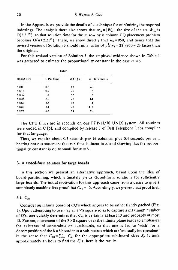
In the Appendix we provide the details of a technique for minimizing the required indexings. The analysis there also shows that w, = 1 W,,,l, the size of the set W,,,, is 0(2.21”), so that solution time for the m row by n column CQ placement problem becomes O(n * 2.21”). There, we show directly that w, = 950, and hence that the revised version of Solution 3 should run a factor of pz/ ws = 2S3/950 = 23 faster than the original.
For this revised version of Solution 3, the empirical evidence shown in Table I
was gathered to estimate the proportionality constant in the case m = 8.
Table I
Board size CPU time # CQ’s # Placements
8x8 0.6 13 40
8x16 0.9 26 18
8x32 1.4 52 2
8x48 2.0 77 64 8x64 2.5 103 4
8X80 3.1 128 472
8x96 3.6 I54 50
The CPU times are in seconds on our PDP-11/70 UNIX system. All routines were coded in C [5], and compiled by release 7 of Bell Telephone Labs compiler for that language.
Thus, we require about 0.5 seconds per 16 columns, plus 0.4 seconds per run, bearing out our statement that run-time is linear in n, and showing that the propor- tionality constant is quite small for m = 8.
3. A closed-form solution for large boards
In this section we present an alternative approach, based upon the idea of board-partitioning, which ultimately yields closed-form solutions for sufficiently large boards. The initial motivation for this approach came from a desire to give a completely machine-free proof that CR, = 13. Accordingly, we present that proof first.
3.1. c,,
Consider an infinite board of CQ’s which appear to be rather tightly packed (Fig. 1). Upon attempting to over-lay an 8 x 8 square so as to capture a maximum number of Q’s, one quickly determines that CR, is certainly at least 13 and probably at most 13. Further, movement of the 8 x 8 square over the infinite plane tends to emphasize the existence of constraints on sub-boards, so that one is led to ‘wish’ for a decomposition of the 8 x 8 board into n sub-boards which are ‘mutually independent’ in the sense that C,, ==Cy=, C’s, for the appropriate sub-board sizes Si. It took approximately an hour to find the S,‘s; here is the result:

The crippled queen placement problem 229
Fig. I.
Theorem 1. C,, 3 13.
Proof. See Fig. 2. Cl
Fig. 2.
Theorem 2. C,, s 13.
Proof. The proof will consist of 3 lemmas:
Lemma 1. C,,s2.
Proof. Up to symmetry, there are 3 possible initial placements (see Fig. 3). Placement
1 clearly permits no additional placements, while 2 and 3 each permit one additional
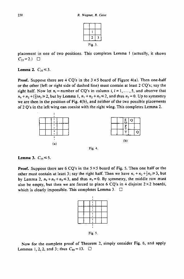
230 R. Wagner, R. Geisr
Fig. 3.
placement in one of two positions. This completes Lemma 1 (actually, it shows
C,,=2.) cl
Lemma 2. CJ5s3.
Proof. Suppose there are 4 CQ’s in the 3 x5 board of Figure 4(a). Then one-half or the other (left or right side of dashed line) must contain at least 2 CQ’s; say the right half. Now let ni = number of CQ’s in column i, i = I,. . . ,5, and observe that n, +n2+(i)n,a2, but by Lemma I, n, +n,+n 3 C 2, and thus n3 = 0. Up to symmetry we are then in the position of Fig. 4(b), and neither of the two possible placements of 2 Q’s in the left wing can coexist with the right wing. This completes Lemma 2.
(b)
Fig. 4.
Lemma 3. C,, 4 5.
Proof. Suppose there are 6 CQ’s in the 5 ~5 board of Fig. 5. Then one half or the other must contain at least 3; say the right half. Then we have n, +n,+$nj> 3, but by Lemma 2, n, + nz + n3 s 3, and thus n3 = 0. By symmetry, the middle row must also be empty, but then we are forced to place 6 CQ’s in 4 disjoint 2 x2 boards, which is clearly impossible. This completes Lemma 3. Cl
Fig. 5.
Now for the complete proof of Theorem 2, simply consider Fig. 6, and apply Lemmas I, 2,2, and 3: thus CR8 = 13. •i

The crippled queen placement problem 231
Fig. 6.
3.2. N,,
Note that in Section 3.1 we established the restrictions of Fig. 7(a). In placing
the maximum number of CQ’s, 13, we must then have w +x +y +z = 13 and hence
w = 2, x = 3, y = 3, and z = 5 (note that this proves Cj5 = 3 and Css = 5). But now
observe that we can put our 3 x3 square in any of the 4 corners! The reader can
easily check that this gives the additional placement restrictions shown in Fig. 7(b).
H x
q ? z
(a) (b)
Fig. 7. (a) w~2: x=-3; ys3; 2~5.
Thus an algorithm for quickly computing N,, presents itelf: fix a choice for the
1 CQ that must appear in the central 2 X2 block, and mark appropriate squares
attacked. (We will multiply by 4 later, that is, we will rotate each solution obtained
from fixing this central block through 90, 180, and 270 degrees, thus producing all
solutions.) For the remaining 8 blocks, move, say counterclockwise, around the
board alternating between the placement of an acceptable (CQ’s not attacked)
pattern for a 3 x3 block (there are 8 such) and the placement of an acceptable
pattern for a 3 x2 block (there are 6 such). When further placement becomes
impossible, change the last-placed pattern to the next on the list of patterns for that
size block, and then proceed forward again.
The possible placements of a single CQ in a 3 ~2 block obviously can be
conveniently indexed 1,2, . . . ,6; the placements of 2 CQ’s in a 3 x3 block are also
conveniently indexed by imposing the numbering system of Fig. 8, so that all eight
placements are given by pairs of consecutive integers (i, i + 1 ), i = 1,2, . . . ,8 (mod 8).
Fig. 8.
232 R. Wagner, R. Ceisr
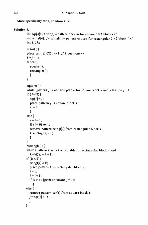
More specifically then, solution 4 is:
Solution 4.
int sqr[4]: /* sqr[i] = pattern chosen for square 3 x3 block i */ int rctngl[4]; /* rctngl[i] = pattern chosen for rectangular 3 x 2 block i */
int i,j, k;
main( ) { place central CQ; /* 1 of 4 positions */ i=j=[;
repeat { square( ); rectangle( );
I 1
square( I{ while (pattern j is not acceptable for square block i and j s 8) j = j + 1; if (jS8){
sqr[i] = j; place pattern j in square block i: k= 1;
1 else {
i=i-1;
if (iSO) exit: remove pattern rctngl[i] from rectangular block i; k = rctngl[ i] + 1;
1
rectangle( ) { while (pattern k is not acceptable for rectangular block i and
k=s6) k=k+l; if (ks6) {
rctngl[i] = k;
place pattern k in rectangular block i;
j= 1;
i=i+l; if (i > 4) {print solution; j = 9;)
. 1
else { remove pattern sqr[i] from square block i; j = sqr[ i] + 1 ;
1 1
The crippled queen placemenr problem 233
Here “place” and “remove” indicate routines to increment and decrement the
counts of attacks on appropriate squares of the 8 x8 board.
In 0.2 seconds of execution time this program produced 10 solutions, and thus
we have IVsI,=40. Again note that all 40 solutions can be seen by simply rotating
each of the 10 produced through 90, 180, and 270 degrees.
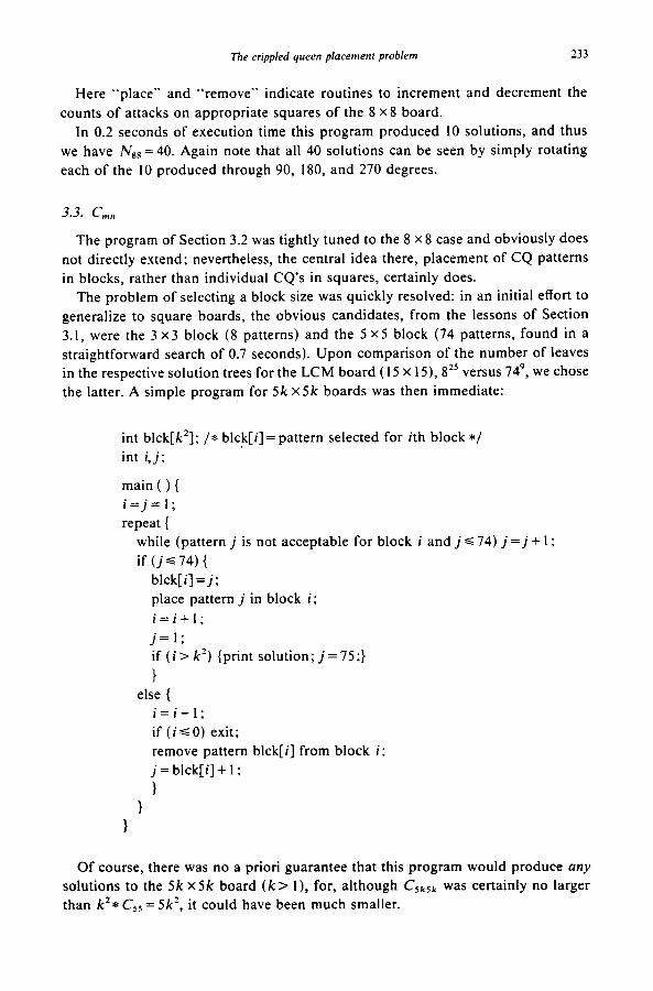
3.3. c,,
The program of Section 3.2 was tightly tuned to the 8 x 8 case and obviously does
not directly extend; nevertheless, the central idea there, placement of CQ patterns
in blocks, rather than individual CQ’s in squares, certainly does.
The problem of selecting a block size was quickly resolved: in an initial effort to
generalize to square boards, the obvious candidates, from the lessons of Section
3.1, were the 3 x3 block (8 patterns) and the 5 x5 block (74 patterns, found in a
straightforward search of 0.7 seconds). Upon comparison of the number of leaves
in the respective solution trees for the LCM board ( I5 x 15), 825 versus 749, we chose
the latter. A simple program for 5k x5k boards was then immediate:
int blck[k*]; /* blck[i] = pattern selected for ith block */
int i,j;
main ( ) {
i=j=l;
repeat {
while (pattern j is not acceptable for block i and j s 74) j = j + 1;
if (jG74) {
blck[ i] = j;
place pattern j in block i;
i=i+l;
j= I;
if (i> k2) {print solution: j =75;}
1 else {
i=i-1;
if (iSO) exit;
remove pattern blck[i] from block i;
j = blck[ i] + 1;
1
1
1
Of course, there was no a priori guarantee that this program would produce any
solutions to the 5k x5k board (k > l), for, although C,,,, was certainly no larger
than k** Cs5 = 5k2, it could have been much smaller.
234 R. Wagner, R. Geist
Further, there were no illusions of improving upon exponential execution time; rather, the hope was that the base and constant terms in the exponential expression would prove to be so small that the barrier to larger boards would be machine address space rather than patience (or life expectancy).
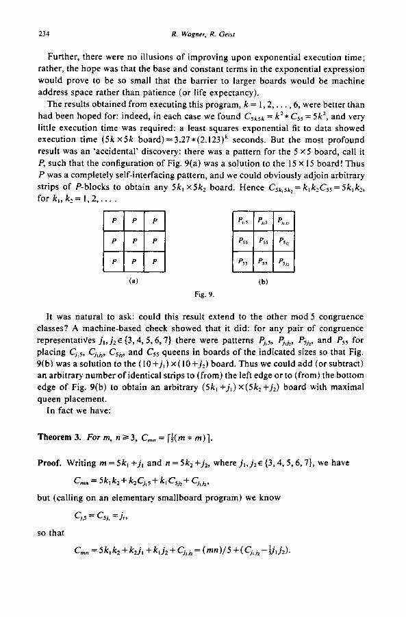
The results obtained from executing this program, k = 1,2, . . . ,6, were better than had been hoped for: indeed, in each case we found C,,,, = k** Css = 5k*, and very little execution time was required: a least squares exponential fit to data showed execution time (5k X5k board) ==3.27*(2.123)k seconds. But the most profound result was an ‘accidental* discovery: there was a pattern for the 5 ~5 board, call it P, such that the configuration of Fig. 9(a) was a solution to the 15 X 15 board! Thus P was a completely self-interfacing pattern, and we could obviously adjoin arbitrary
strips of P-blocks to obtain any 5k, X5k, board. Hence C5k,+ = k, k&, = 5k, k2,
fork,,k,=1,2 ,....
It was natural to ask: could this result extend to the other mod 5 congruence classes? A machine-based check showed that it did: for any pair of congruence representatives jr, j, E {3,4,5,6,7} there were patterns Pj,5, Pj,jz, P5j2, and Ps5 for placing Cj,s, C’,j*, Csj,, and C,, queens in boards of the indicated sizes SO that Fig. 9(b) was a solution to the (IO +j,) x (IO +j,) board. Thus we could add (or subtract) an arbitrary number of identical strips to (from) the left edge or to (from) the bottom edge of Fig. 9(b) to obtain an arbitrary (5k, +j,) x(5k,+jJ board with maximal queen placement.
In fact we have:
Theorem 3. For m, n 23, C,, = [f(m * m)].
Proof. Writing m = 5k, +j, and n = 5k2 +j,, where jr, jzE {3,4,5,6,7}, we have
C,,=5k,k*+k,Cj,~+k,CSi,+Cj,h,
but (calling on an elementary smallboard program) we know
cj,5 = C5j, =ji,
so that
C WI” =5k,k,+k,j, +k~j2+C’,jz=(mn)/5+(Cj,~-$,j2).

The crippled queen placement problem 235
Finally, calling on ‘smallboard’ again, we find 0 < Cj, j2 - $,j2 < 1, giving the desired
result. Cl
For the sake of completeness, we note that C,. = [f( 1 * n)], and G, = [a@* n)l.
3.4. N,,,,
There was yet another ‘accidental’ discovery made in running the program of
Section 3.3: N,S ,5 = NZolO= NZsZ5 = N,,,, = SO! This (the constancy) was indeed
unexpected, but, upon viewing the individual solutions, the cause of the constancy,
as well as a method for generalization to N,,,, became clear.
We need some additional notation. For each solution to an m x n board, let us
define an associated pattern array as follows: first, index the solutions to each jr x j,
board, jr jZ E {3,4,5,6,7} (this does require some straightforward machine computa-
tion with worst case 7 x7: 5 minutes); then write m =5k, +j,, n =5k,+j,, and
partition the m x n solution pattern into (k, + 1) x ( k2 + 1) blocks, as shown in Fig.
10. Replacing each pattern of CQ’s with its associated index, we have a (k, + 1) X
( k2 + 1) array of pattern indices which conveniently represents the m x n solution.
j,XS . . . il x5 il xi2
5x5 . . . 5x5 5xj,
.
. .
. .
I 15x5 . . . 5x5 5xjz
Fig. 10.
Theorem 4. For euery r L 4, for every s 2 4, any pattern array of dimension r x s will have interior rows (rows other than first and last) which are all identical and interior columns which are all identical.
Thus, by removing interior rows and columns, we see that any placement of CQ’s
on a large board is necessarily a unique and trivial extension, obtained by replicating
interior rows and/or columns, of a placement on a small board whose dimensions
have the same mod 5 congruence classes as those of the large board.
Proof of Theorem 4. We use a nested induction: first consider the case r = 4. The theorem was verified for the case s = 4 by direct computer generation of all boards
236 R. Wagner. R. Geisr
having each dimension between 18 and 22, inclusive. Since an efficient block- placement program was used, the total execution time required here was roughly 7 minutes. Of course, the case r = 4, s = 4 chronologically preceded the theorem itself and was the basis of all the mathematical development.
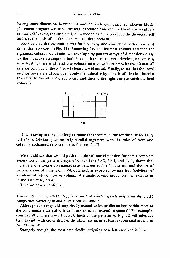
Now assume the theorem is true for 4~ s < s,,, and consider a pattern array of dimension r X (sO + 1) (Fig. 11). Removing first the leftmost column and then the rightmost column, we obtain two over-lapping pattern arrays of dimensions r x s,,. By the inductive assumption, both have all interior columns identical, but since s0 is at least 4, there is at least one column interior to both r xso boards; hence all interior columns of the r x (so + 1) board are identical. Finally, to see that the (two) interior rows are still identical, apply the inductive hypothesis of identical interior rows first to the left r xso sub-board and then to the right one (to catch the final column).
12 . . so SrJ + I
ElEl3l
Fig. I I.
Now (moving to the outer loop) assume the theorem is true for the case 4~ rs r. (all sa 4). Obviously an entirely parallel argument with the roles of rows and columns exchanged now completes the proof. q
We should say that we did push this (down) one dimension further: a complete generation of the pattern arrays of dimensions 3 x3, 3 x4, and 4 x3, shows that there is a one-to-one correspondence between each of these sets and the set of pattern arrays of dimension 4 x4, obtained, as expected, by insertion (deletion) of an identical interior row or column. A straightforward induction then extends us to the 3xs case, s>4.
Thus we have established:
Theorem 5. For m, n 2 13, N,,,, is a constant which depends only upon the mod 5 congruence classes of m and n, as given in Table 2.
Although constancy did empirically extend to lower dimensions within most of the congruence class pairs, it definitely does not extend in general! For example, consider NJn where n E 5 (mod 5). Each of the patterns of Fig. 12 will interface (end to end) with either itself or the other, giving us at least exponential growth in Nsn as n + +a~
Strangely enough, the most empirically intriguing case left unsolved is 8 x n.

The crippled queen placemenr problem 237
Table 2
N mn
n(mod 5)
3 4 5 6 7
3 24 4 46 14 2
4 4 2 44 20 10
m(mod5) 5 46 44 50 50 52
6 14 20 50 2 4
7 2 IO 52 4 16
Fig. 12.
4. Comparisons
We have presented several approaches to the solution of a novel generalization
of the &queens problem. In effect, we have tried to show not one ‘best’ solution,
but a ‘tree of choices’ leading to a set of solutions with different properties. This
tree of choices can be described by the outline shown in Table 3.
Table 3
Run time
8x8 8xn mxn
1. Exhaustive search
2. Branch and bound
3. Dynamic programming
(a) 0(n(p,)3)
(b) O(nw,,,) 4. Partitioned board
(a) 8x8
(b) 5kx5k
(c) mxn;m,n~13
240min -
5 set WC”) O(Crn”)
n=lSin IOmin
23 times slower than 3b (est)
0.6 set 0.4 f n/32 set O(n 2.21rn)
0.2sec - - 3.27*2.123k
0 set
We can (rather informally) also characterize the amount of time or thought
(estimated by the individuals involved) expended on each solution, see Table 4.
In Table 4, * denotes the following: Some additional information was acquired
as a result of previous computational experience with the problem by individuals
who generated these solutions:
238 R. Wagner, R. Geisr
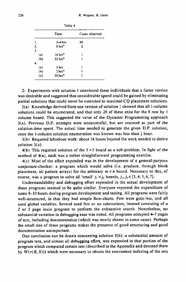
Table 4
Time Cases observed
I. 34 hrs 10 2. 8 hrs* 2 3.
(a) 16 hrs* I @I 32 hrs* I
4.
Ii; 3 hrs I 2 hrs* 1
(cl 30 hrs* 1
2: Experiments with solution 1 convinced these individuals that a faster version was desirable and suggested that considerable speed could be gained by eliminating partial solutions that could never be extended to maximal-CQ placement solutions.
3(a) Knowledge derived from one version of solution 1 showed that all l-column solutions could be enumerated, and that only 28 of these exist for the 8 row by 1 column board. This suggested the value of the Dynamic Programming approach 3(a). Previous D.P. attempts were unsuccessful, but are counted as part of the solution-time spent. The actual time needed to generate the given D.P. solution, once the l-column solution enumeration was known was less than i hour.
3(b) Required laborious work: about 16 hours beyond the work needed to derive solution 3(a).
4(b) This required solution of the 5 ~5 board as a sub-problem. In light of the method of 4(a), each was a rather straightforward programming exercise.
4(c) Most of the effort expended was in the development of a general-purpose conjecture-checker: a program which would solve (i.e. produce, through block placement, all pattern arrays) for the arbitrary m x n board. Necessary to this, of course, was a program to solve all ‘small’ j, x j, boards, j,, j, E {3,4,5,6,7}.
Understandability and debugging effort expended in the actual development of these programs seemed to be quite similar. Everyone reported the expenditure of some 8-10 hours during program development and testing. All programs were fairly well-structured, in that they had simple flow-charts. Few were goto-less, and all used global variables. Several used few or no subroutines, instead consisting of a 2 or 3 page main program to perform the exhaustive search. Nonetheless, no substantial variation in debugging ease was noted. All programs occupied 67 pages of text, including documentation (which was nearly absent in some cases). Perhaps the small size of these programs makes the presence of good structuring and good documentation unimportant.
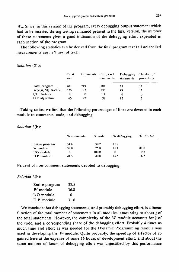
One conclusion can be drawn concerning solution 3(b): a substantial amount of program text, and almost all debugging effort, was expended in that portion of the program which computed certain sets (described in the Appendix and denoted there by W( r( R, S))) which were necessary to obtain the convenient indexing of the sets
The crippled queen placement problem 239
W,,,. Since, in this version of the program, every debugging output statement which
had to be inserted during testing remained present in the final version, the number
of these statements gives a good indication of the debugging effort expended in
each section of the program.
The following statistics can be derived from the final program text (all unlabelled
measurements are in ‘lines’ of text):
Solution (3)b:
Total
size
Comments Size, excl Debugging Number of
comments statements procedures
Total program 401 219 182 61 13
W(r(R, S)) module 325 192 133 49 II
I/O modules II 0 II 0 0
D.P. algorithm 65 27 38 12 2
Taking ratios, we find that the following percentages of lines are devoted in each
module to comments, code, and debugging.
Soluhon 3(b):
% comments % code % debugging % of total
Entire program 54.6 30.2 15.2
W module 59.0 25.8 15.1 81.0
I/O module 0 100.0 0 2.1
D.P. module 41.5 40.0 18.5 16.2
Percent of non-comment statements devoted to debugging:
Solution 3(b):
Entire program 33.5
W module 36.8
I/O module 0
D.P. module 31.6
We conclude that debugging statements, and probably debugging effort, is a linear
function of the total number of statements in all modules, amounting to about f of
the total statements. However, the complexity of the W module accounts for $ of
the code, and a corresponding share of the debugging effort. Probably 4 times as
much time and effort as was needed for the Dynamic Programming module was
used in developing the W-module. Quite probably, the speedup of a factor of 23
gained here at the expense of some 16 hours of development effort, and about the
same number of hours of debugging effort was unjustified by this performance

240 R. Wagner, R. Geisr
improvement. On the other hand, no data on the eKort needed to develop a more
straightforward implementation of the D.P. algorithm, running in time O( p’,), is
available. (It could be estimated at about f the time and effort needed for development
of the current W-module.)
For comparison, we present program size and complexity statistics for the fastest
implementation of solution 2 (a program written by Charles Poirier):
Solution 2 :
Total size Comments Size, excl
comments
Total program 168 93 75
I/O module 30 4 26
Main algorithm 138 89 49
This program includes no procedures, and no debugging statements. Its text is also
complicated by the presence of 3 goto statements. We note that, when debugging
statements and I/O-related statements are excluded from solution 3(b)‘s statistics,
we get the following comparison:
Solution 3(b): 110 lines, 84 in W module,
Solution 2: 49 lines.
Had the W module been replaced by a slower version to implement solution 3(a),
occupying about 30 lines of code, the comparison would be:
Solution 3(a): 56,
Solution 2: 49.
Thus, the programs would be of approximately the same size, and of approximately
the same complexity. The size of solution 3(b) is in large part due to its complex
W module, and this added complexity results from a choice made at the ‘second
level’ of the choice tree.
Of all the solutions to the 8 x8 board, 4(a) required the fewest lines of code and
the least amount of execution time. Nevertheless, when development time and
requisite documentation, including theorem statements and proofs, are added, the
solution becomes one of the longest and most time-consuming of all, and thus, as
a ‘stand-alone’ effort, 4(a) is not an unqualified success. Of course, this is somewhat
unfair in that 4(a) ultimately led to the closed-form solutions for C,,,, (all m, n) and
N,,,, (m, n 3 13), and the value of these solutions must also be weighed when making
the comparisons.
We can, for this problem, document the fact that effort expended at the outermost
level of the program development hierarchy, namely, while deciding on an overall
approach to the problem, produces the greatest improvement in program perform-
ance. Furthermore, such effort seems to leave program complexity unaffected.

The crippled queen placement problem 241
Although the resulting program may operate using principles that are not apparent,
and which need proof, the actual code produced uses these principles in straightfor-
ward fashion.
5. Conclusions
We have presented in this paper a fairly detailed description of the design process
as it applies to the solution of one problem. In the course of the solution, the
designer must make choices at several levels of detail. Initially, a choice of solution
strategy is needed. We have shown the initial cost differences incurred in making
this strategic choice:
1. Straightforward, in analogy with 8 queens: 240 minutes,
2. Branch and bound: 4.8 seconds,
3. Dynamic programming: 0.6 seconds,
4. Board partitioning: 0.2 seconds.
Other measures of solution quality including program complexity are either essen-
tially constant, or improve in order from choice 1 through choice 4.
However, our best attempts to guide further choices at lower levels of detail via
estimates of the improvements to be gained have to be judged failures:
Choice 1 vs 2: No easy estimate of the improvement to be expected as a result of
a branch-and-bound solution was possible. It was far easier to make the minor
change in solution 1 that produced solution 2, and see what happened than to
perform any a priori mathematical analysis.
Choice 3a vs 3b: Initially, we thought that relatively few triples of adjacent column-
patterns were mutually compatible. We had no notion of how large W,,, was. The
mathematical analysis presented in the Appendix was carried out in part to determine
this quantity. Once completed, we decided to develop the O(n x w,) algorithm
(which was fairly straightforward once the analysis giving enumeration of w, had
been done). Yet the effort expended to obtain Table 1 was unjustified by the linear
factor of 23 improvement we gained.
Choice 4: A priori estimates of the gains to be made at each stage of the development
of solution 4 were, at best, of a probabilistic and subjective nature. Although the
derivation of a closed-form solution remained feasible at each stage of the develop-
ment, the possibility of no return (other than insight into the complexity of the
problem) on time invested also remained. The chief merit of solution 4 (all parts)
is that it is representative of a research technique which we feel will become
increasingly important in both mathematics and computer science: machine-gener-
ation of theorem statements (the ‘accidents’ of Section 3), followed by their inductive
proofs.

21’ R. Wagner, R. Geisr
We hope that documenting the issues which arose during the design of one non-trivial program will prove valuable to researchers in program methodology. They may be of value also to designers of Computer Science curricula. We feel that this study shows the value of a general background in mathematical problem solving when attacking novel problems.
When mathematical reasoning is coupled with use of the computer to resolve conjectures, a powerful problem solving mode results. This produces high-quality software products.
Appendix A. An indexing of the set of compatible column-pattern triples
Solution 3 requires indexing over the set W,,, = {(R, S, T): (RIS) and (S(T) and (R 11 T)}. Here we show how to compute a convenient bijection h: I,,, + W,,,, where Z,={O, I,..., k- 1) and w, = 1 W,,,\, the number of objects in the set W,,,. The
techniques used to develop this bijection can be exploited in two ways: (1) We can easily develop a tabulation technique that, for any m, gives W,,,; and (2) We can design computer programs that compute the sets W( r(R, S)) =
{r(S, T): (R, S, T) E W,} where r: X,,, + Z,, is a bijection with domain
X,,, = {(R, S): R/S}, with x, = Ix,,,~.
Thus, the indexing over all T such that (R, S, T) E W, is reduced to indexing over all elements of W(r(R, S)).
A.I. The set X,,, ={(R, S): RIS}
We proceed to derive recursive formulas for the number of solutions to an i ~2 board, for i=l,..., m. Let LO(i) be the number of different legal CQ placements possible on the i ~2 board, without inter-CQ attack. Consider row i of the board. Legal CQ placements include some with no CQ’s in row i, others with a CQ in column 1, or in column 2, but none with a CQ in both columns.
Let PO(i) be the number of solutions to the i x2 board with no CQ’s in row i, e(i) be the number of solutions to the i x2 board with a CQ in row i column j, forjE{l,2}. Then:
LO(i)=PO(i)+Pl(i)+P2(i),
PO(i) = LO(i- 1) and PI(i) = P2(i).
To develop a recursive formula for Pl( i), note that a CQ in row i column 1 attacks squares so that the squares which remain available for CQ occupancy form a 2 column board whose 1st column contains i - 3 rows, and whose second contains i - 2 (See Fig. Al). Let Ll (i) be the number of legal CQ solutions possible on a 2-column board, one of whose columns is i rows long, the other i - 1 rows long. Then Pl(i)=P2(i)=Ll(i-2).

The crippled queen placement problem 243
2 I
row i: Q i-l:
i-2: x
i-3: X X
Fig. Al. Q represents a CQ, - an attacked square, and x an unattacked unoccupied square.
Now Ll( i) can be analyzed similarly: its ith row either holds no CQ, giving LO( i - 1) solutions, or it holds one CQ, giving Pl (i) = P2( i) = Ll (i - 2) solutions. Thus, we are led to the following formulation:
LO(i)=LO(i-1)+2Ll(i-2), (A.0)
Ll(i)=LO(i-l)+Ll(i-2), (A.1)
and thus
LO(i)=Ll(i)+Ll(i-2). (A.2)
We note that LO(O) = 1 (There is one solution-the empty board-for the board with no rows), and Ll(0) = 1 for the same reason. Similarly, the reader can verify directly that LO( 1) = 3 and Ll(1) = 2. Using (A.1) and (A.2) we can then generate Table Al. Thus x8= 193, which is smaller than 4*(~(8))~, since p(8) = 28 = the number of 8 x 1 solutions.
Table Al
i Ll(i) LO(i)
0 I I I 2 3 2 4 5
3 7 9 4 13 17 5 24 31
6 44 57 7 81 105
8 149 193
Note that closed-form expressions for LO(i) and Ll( i) can be developed: by substituting (A.2) into (A.1) we obtain Ll(i)=Ll(i-l)+Ll(i-2)+Ll(i-3), and similarly by combining (A.1) and (A.2) and substituting into (A.0) we obtain LO(i) = LO( i - 1) + LO( i - 2) + LO( i - 3). Each linear difference equation thus has characteristic polynomial X3-X2-X - 1 whose 3 roots, S,, S,, and S,, can be expressed in terms of radicals. The general closed-form expression is then LO(i)=
C,Si + C& + C,S: where the coefficients are determined by the initial values. (Of

244 R. Wagner, R. Geist
course, the same is true for Ll (i).) In particular, since the real root is approximately 1.839286 and the two complex roots have an approximate norm of 0.7373527, we can say that x, is 0( 1.84” ).
To develop the function r, we first describe a simple representation of the 2-column solutions by means of strings of digits. Each 2-column solution has the property that its ith row contains either 0 or 1 CQ’s. Let S be a string of digits over the alphabet (0, I, 2). Then S describes an ISI x2 pattern of CQ placements, by the correspondence; row i of the solution contains one CQ in column j (j = 1 or 2) if
the ith digit of S, S(i), satisfies S(i) =j. If S(i) = 0, the solution corresponding to string S has no CQ in row i.
Now, some strings S as above describe legal solutions, while others do not. Let us define the function f on strings S as follows:
Then
f(S) = the number of legal solution strings T which are lexicographically ordered less than S, if S is a legal solution string; undefined, otherwise.
f(W =f(S), f(lOS)=~O(ISI+I)+g(l,S), f(2oS)=Lo(~s~+l)+Pl(~s~+2)+g(2,s)=Lo(~s~+l)+Ll(~s~)+g(2,s), f( xyS) = undefined otherwise,
where, for i = 1,2, g( i, S) denotes the number of strings which precede S on a board with ISI rows which has one square removed from column i, row ISI. So
g(i, OS) =f(S), g(3 - i, is) = LO(lSl, t-f(S), g( i, yS) = undefined otherwise.
Furthermore,
f(0) =O=f(h) where A = the null string,
f(l)= 1, f(2) = 2.
The first few solution strings, and their corresponding f values can be tabulated using Table Al, see Table A2.
Each solution string S can be preceded by any number of 0 digits to modify it to describe solutions for values of the row index i > ISI. Since f(OS) = f(S), the value off(S) is independent of i, so long as I ‘3 ISI. Furthermore, a deterministic finite state machine can be designed to read string S (from left to right), determine if S represents a legal solution, and develop the value of f(S) (see Fig. A2).
Note that we can now define t: if (R, S)E X,,, then we can write R =
(Rm Rot-,, . . . , R,) where each Ri = 2, if a CQ appears in row i, and Ri = 0, otherwise. Similarly S = (S,, Sm...,, . . . , S,) where Si = 1, if a CQ appears in row i, and Si = 0
otherwise.Then r(R,S)=f((R,+S,,,)(R,_,+S,,,_,)*-*(R,+S,)).

The crippled queen placement problem 245
Table A2
String S f(S)
0 0
I I
2 2
IO 3 20 4
100 5
102 6
200 7
201 8
1000 9
Fig. AZ. A deterministic finite-state machine to calculate F(S); start state: 0. Initially Q=O: on termina-
tion Q holds F(S).-A: add LO(J-I) to Q. B: add 151(J) to Q, where J is the number of digits between
the read-head and right end of string, inclusive.
A.2. Theset W,,,={(R,S,T):RIS,RIIT,SjT}
We begin in much the same way as in Section A. 1 to develop the number of solutions
for a 3-column by i-row board. Somewhat more complexity results, since more CQ
placements are possible in row i, and in addition, more distinct board shapes must be
considered. See Fig. A3.
column 321 321 321 321 32 I
- Q- Q- - row i+l --- Q-- ___ ___ __Q
row i xxx --X x-x - x- X--
row i-l xxx - x- xxx xxx - x-
row i-2 xxx xxx xxx xxx
shape 0 shape I shape 13 shape 2 shape 3
Fig. A3. 3-column by i-row board shapes. Status of board squares are shown by symbols as
follows: Q=occupied, -=attacked or off board, x=available.

246 R. Wagner, R. Geist
Let L3s(i) be the number of legal CQ placements for a board with i rows and 3 columns, in which certain squares in rows i and i-l are not ‘available’ for CQ placement. Specifically:
available in row s i i-l
0 all all 1 I 2 2 2 all 3 3 2
13 1.3 all
Then, from Fig. A3,
L3O(i)=L3O(i-l)+L33(i-I)+L3l3(i-2)+L3l(i-l),
where the summands correspond respectively to the case where there are 0 CQ’s in row i, or one CQ in columns 1, 2, or 3 of row i. Now L33( i)=L31( i)=
L32(i-l)+L32(i-2), where the summands correspond to 0 or I CQ in the only available square of row i. Similarly, L32(i)=L30( i-l)+L313(i-2), and L313(i)= L3O(i-l)+L33(i-l)+L3l(i-l), for no CQ’s or a CQ in columns I or 3 respectively. These equations can then be reduced to:
L3O(i)=L3O(i-l)+3L3O(i-3)+4L3O(i-4)+4L3O(i-5)+2L3O(i-6).
Now the characteristic polynomial y6-y5-3y3-4y2-4y-2 has real roots 2.202044 and -0.667283 (approx.) and two pairs of complex roots with norms 0.8678813 and 1.34427 (approx.). Thus, as with x, earlier, we can say w,=L30(m)=0(2.21m). (See also Table A3.)
Table A3
i L313(i) L30( i) L33(i) L32(i)
I 3 4 2 2 2 8 9 3 5 3 15 18 7 12 4 32 40 17 26 5 74 89 38 55 6 165 197 81 I21 7 359 433 176 271 8 785 950 392 598
This analysis, conducted before proceeding with the development of algorithms to enumerate W,,,, showed:
(I) For m=8, w,=950, which is proportional to the execution time of solution 3 if W,,, is enumerated. The corresponding time of ~(8)~=28~=21 952 is a factor of more than 23 greater. Thus it seemed worthwhile to proceed with the development, presented in Section A.l, of the finite state machine used to compute the function f(S), where S represents any IS/x2 solution.

The crippled queen placemenr problem 247
(2) Solution 3 will require time 0( n * 2.21”) to solve the general rn row by n
column CQ placement problem.
A.3. An algorithm to compute the sets W(r(R, S))={r(S, T): (R, S, T)E W,,,}
The general approach is to generate strings of digits over (0, I, 2,3} representing
solutions to the ix3 board, using a collection of recursive subroutines. As each digit
Si of a string S is generated, Si is translated (by indexing into a table) into a pair
(T,, K,) of digits, representing S as two over-lapping 2-column solutions. Specifi-
cally, Si>O indicates the presence in S of a CQ in column Si, row i. The corresponding
T, value is 0 if Si=O or Si=3, and Tl=Si otherwise. Similarly, Tz is 0 if Si=O or Si= I, and T,,=S,-1 otherwise. The sequences (T,,) and (T,,) can then be fed into
the finite state machine presented in Section A. 1 to produce the integer pair sequence
(f(T,),f( Ti2)). When string S represents the member (S,, Sz, S,) of W,,,,f( T,,)=
r((S, Sd) and f( Tj2)= r((L Sd). In practice, the strings S are generated, digit by digit, without backtracking, so
that whenever a string S has been produced it is known that there is some suffix Q
of digits such that SQE W,,,. This suggests that the digits Tii, and Tii, be presented
in parallel to two separate copies of the f-computing FSM. Whenever ISI=m, the
values computed thus far by each FSM copy are used asf( K,) andf( Tii2) respectively.
A record is kept of the state of each FSM (including its value off), so that digits
of a T-string can be removed, and a new suffix substituted for them, without
recomputing f on the unchanged prefix of the T-string. Our W-enumeration
algorithm then pushes f( Tii2) onto queue W[f( T,,)], after initializing all queues
W[i] empty.
There remains the mathematical problem of producing recursive subroutines to
generate strings SE W,,,, without backtracking. This problem was solved by examin-
ing the recursive equations for L3s( i), together with their derivations. One recursive
routine, TRY~s(~), was built for each shape s. The job of routine TRY~S( i) is to
produce every solution to the shape s board with i rows. Each digit S, produced is
fed, along with i, to routine o(S, i), which translates S, into K, and T,2, and feeds
it as digit m-i+1 of an m digit string (rk) to FSM copy k. Routine -rRY3s(i) produces the first legal value V, of digit Si, and then calls another rRYJs’( i-.I( V,))
routine to produce all solutions having initial digit Si= Vi before producing any
solutions with Si> Vti (Here, J( Vi)c{ 1,2,3}. J( V,) is generated along with the value
vi.) For example, routine ~~~313(i) is:
if (i>O) { Q(0, i); TRY~O( i - 1);
o(l, i); Q(0, i-l);rnY32(i-2); Q(3, i-l): C?(O, i-2);Tnv32(i-3);
Q(3,i);Q(O,i-l);~~~32(i-2);Q(1,i-l);Q(O,i-2);f~Y32(i-3);}
else soln( ); return;

248 R. Wagner, R. Geisr
Routine soln( ) is responsible for updating queues W[i], and recording the number
of CQ’s in columns 1 and 2. Routine Q keeps track of the number of CQ’s placed
into columns I and 2 by each solution-string S. Communication among routines
o( ) and soln( ) takes place using global variables, and the states of FSM copy j
are recorded in a statically allocated global array QM at QM[i][j], so that the
replacement of a suffix of a 2-column string by a different suffix is simple, for all
earlier states of each FSM copy are accessible to routine 0 ( ). This recursive
technique produces a constant number of subroutine calls for each digit of every
solution-string it produces. However, it produces a tree T of subroutine calls whose
leaves represent solution strings by the correspondence: The solution represented
by leaf L is given by the sequence of labels of tree arcs on the unique path from
the tree root to I., where each tree arc is labelled by a digit. This tree of solution
strings has no more than 2 * w, arcs, total, for it has at most w,,, internal nodes,
where w,,, is the number of leaves of T, The entire solution 3, including computation
of the sets W( r( R, S)), thus requires time O( w,,, * (n+l)) to solve the rn row, n
column CQ placement problem.
References
[I] W.R. Ball, Marhemarical Recreations and Essays (Macmillan, New York, I Ith ed., 1960).
[2] R. Bellman, D.vnamic Programming (Princeton University Press, Princeton, 1957).
[3] J.R. Bitner and EM. Reingold, Backtrack programming techniques, Comm. ACM IS (1975) 651-656. [4] G. Papadimitriou and K. Steiglitz, Combinatorial Opfimkarion (Prentice-Hall, Englewood Cliffs, NJ,
1982).
[5] D.M. Ritchie, S.C. Johnson, M.E. Link and B.W. Kemigham, The C programming language, Bell
Sysf. Tech. J. 57 (6, Part 2) (1978) 1991-2020.