The coupled variability of the ... - seminar.censam.sg. Jun Wei.pdf · Why develop a coupled model...
18
Jun Wei 1,3 ,Paola Malanotte-Rizzoli 2,3 and Elfatih Eltahir 2,3 1 Peking University, China 2 Massachusetts Institute of Technology, USA 3 Singapore-MIT Alliance for Research and Technology, Singapore Singapore 2017. 06. 29 The coupled variability of the regional climate in the South China Sea
Transcript of The coupled variability of the ... - seminar.censam.sg. Jun Wei.pdf · Why develop a coupled model...
Jun Wei1,3,Paola Malanotte-Rizzoli2,3 and Elfatih Eltahir2,3
1
Peking University, China 2
Massachusetts Institute of Technology, USA 3
Singapore-MIT Alliance for Research and Technology, Singapore
Singapore
2017. 06. 29
The coupled variability of the regional climate
in the South China Sea
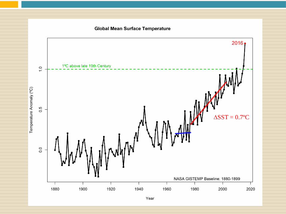
∆SST = 0.7ºC

E
Oceanic bridge Atmospheric bridge
Remote forcing to the SCS

Why develop a coupled model (RegCM–FVCOM)?
RegCM3 – FVCOM: 5 ~ 200 km
(coupled)
Air-Sea coupling: Xue et al. (2014)
Seasonal variability: Wei et al. (2014a)
Interannual variability: Wei et al. (2014b)
Decadal variability: Wei et al. (2016)
MC-RegCM: by Prof. Eltahir’s group
A Regional Climate Model (60 km)
Maritime Continent (MC)
MC-FVCOM: by Prof. Rizzoli’s group (ocean only)
Wei et al. (2011)
Chen et al. (2011, 2012, 2014)
Tkalich et al. (2012)
Xu and Rizzoli (2013)
Thompsom et al. (2015, 2016)
Sun et al. (2017, in press)

Do i=1, N, int_2
Call fromcpl
Parallel running
Node (1) …… Node (20)
Call intocpl
End
Enddo In
terpo
lation
Wind
Fluxes
Coupler Do i=1, N, int_1
Call fromcpl
Parallel running
Node (1) …… Node (12)
Call intocpl
End
Enddo
SST
Internal mode
RegCM3 FVCOM
Wind
Fluxes
SST
Negative feedback: SST – Heat flux (Xue et al. 2014)
Positive feedback: Wind – Evaporation – SST (Wei et al. 2016)

Methodology to separate the oceanic and atmospheric forcing
∆𝑆𝑆𝑇 = − 𝑢𝜕𝑇
𝜕𝑥+ 𝑣
𝜕𝑇
𝜕𝑦+ 𝑤
𝜕𝑇
𝜕𝑧
𝐴𝐷𝑉
+ 𝜕
𝜕𝑧𝐾ℎ
𝜕𝑇
𝜕𝑧
𝑀𝐼𝑋
+ 𝑄
ℎ𝜌0𝐶𝑝
𝐻𝐹𝑋
Luzon inflow Wind and heat flux
(Oceanic forcing) (Atmospheric forcing)
∆KE = − 𝑢𝜕𝐾
𝜕𝑥+ 𝑣
𝜕𝐾
𝜕𝑦+ 𝑤
𝜕𝐾
𝜕𝑧
𝐴𝐷𝑉
− 𝑢𝜕𝑝
𝜕𝑥+ 𝑣
𝜕𝑝
𝜕𝑦
𝑃𝑊𝐻
+ 𝑢𝜕𝜏
𝜕𝑧+ 𝑣
𝜕𝜏
𝜕𝑧
𝑊𝑁𝐷
Temperature Equation
Momentum Equation
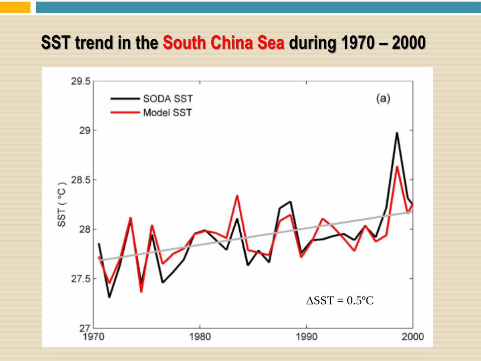
SST trend in the South China Sea during 1970 – 2000
∆SST = 0.5ºC

Coupled model (TL_∆SST) SODA re-analysis (TL_∆SST)
A
B
C

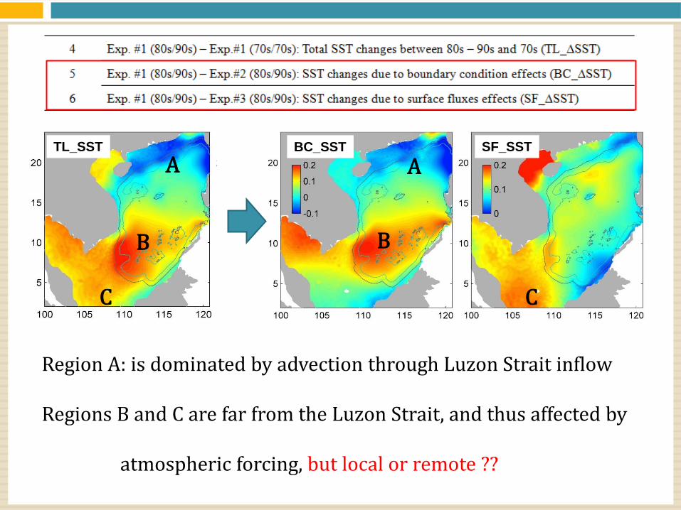
SF_SST TL_SST BC_SST
∆𝑆𝑆𝑇
= − 𝑢𝜕𝑇
𝜕𝑥+ 𝑣
𝜕𝑇
𝜕𝑦
𝐴𝐷𝑉
+ 𝜕
𝜕𝑧𝐾ℎ
𝜕𝑇
𝜕𝑧
𝑀𝐼𝑋
+ 𝑄
ℎ𝜌0𝐶𝑝
𝐻𝐹𝑋
BC_∆SST SF_ ∆SST
SF_SST TL_SST BC_SST
A A
B B
C C
Region A: is dominated by advection through Luzon Strait inflow Regions B and C are far from the Luzon Strait, and thus affected by atmospheric forcing, but local or remote ??

Region A:
ENSO signal goes to SCS via Luzon Strait
Region B:
ENSO affects SST through trade winds
Region C:
SST is driven by local heat flux variability
TL_SST
A
B
C
For SST variability:

TL_KE BC_KE
The total surface KE is basically identical to BC_KE clearly
showing the SCSTF
Surface Kinetic Energy
SF_KE

SF_KE TL_KE BC_KE
The effect of atmospheric forcing (SF) on the circulation is one order of magnitude smaller than that of the oceanic boundary condition (BC).
Barotropic Kinetic Energy

SF_KE TL_KE BC_KE
∆KE
= − 𝑢𝜕𝐾
𝜕𝑥+ 𝑣
𝜕𝐾
𝜕𝑦
𝐴𝐷𝑉
− 𝑢𝜕𝑝
𝜕𝑥+ 𝑣
𝜕𝑝
𝜕𝑦
𝑃𝑊𝐻
+ 𝑢𝜕𝜏
𝜕𝑧+ 𝑣
𝜕𝜏
𝜕𝑧
𝑊𝑁𝐷
BC_∆KE SF_ ∆KE
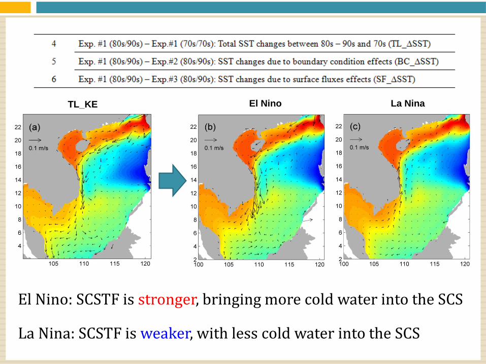
La Nina TL_KE El Nino
El Nino: SCSTF is stronger, bringing more cold water into the SCS
La Nina: SCSTF is weaker, with less cold water into the SCS

Atmos. bridge
Summary:
0 0.5 10
0.5
1
0
0.1
0.2
0.3
0.4
ºC
TL_SST
Remote

Summary:
0 0.5 10
0.5
1
0
0.1
0.2
0.3
0.4
ºC
TL_SST
Local
Remote
Remote
1. The Northern SCS is affected by
remote forcing via Luzon Strait
(Oceanic bridge).
2. The central SCS can be affected
by remote forcing as well, but
through the trade wind variability
(Atmospheric bridge).
3. The shallow Sunda shelf in the
Southern SCS is driven by local
heat flux – SST interactions.
4. The circulation in the SCS is
dominated by the Luzon inflow
(Oceanic bridge).
A
B
C
Thanks!
W
W
C
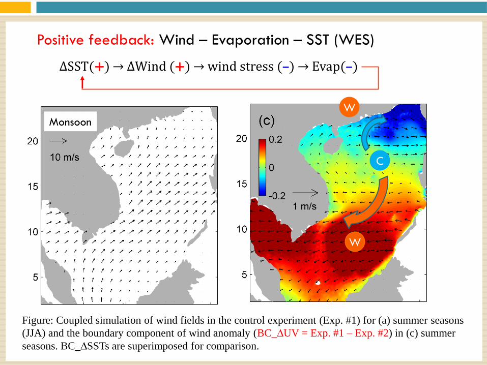
Figure: Coupled simulation of wind fields in the control experiment (Exp. #1) for (a) summer seasons
(JJA) and the boundary component of wind anomaly (BC_∆UV = Exp. #1 – Exp. #2) in (c) summer
seasons. BC_∆SSTs are superimposed for comparison.
Positive feedback: Wind – Evaporation – SST (WES)
Monsoon
∆SST(+) → ∆Wind (+) → wind stress (–) → Evap(–)