J. theor. Biol. (1995) 173, 217–230

0022–5193/95/070217+14 $08.00/0 7 1995 Academic Press Limited

The Coupled Logistic Map: A Simple Model for the Effects of

Spatial Heterogeneity on Population Dynamics

A L. L

Department of Zoology, University of Oxford, South Parks Road, Oxford OX1 3PS, U.K.

(Received on 3 August 1993, Accepted in revised form on 19 October 1994)

A simple model consisting of two diffusively coupled logistic maps is used to examine the effects of spatialheterogeneity on population dynamics. Examining the dynamic behaviour of the model using numericalmethods, a wide range of behaviours are observed. It is shown that the coupling can stabilize individuallychaotic populations, and that under different circumstances the coupling can cause individually stableperiodic populations to undergo more complex behaviour. The system exhibits multiple attractors whenthe qualitative dynamics of the system depend on the initial conditions. Sudden changes in the structureof the attractors are seen for small changes in the parameters; these changes are known as crises. Transientand intermittent behaviours are observed. The implications of all these behaviours for populations arediscussed. A linear coupling of the two maps is also considered which leads to counterintuitive behaviour,with chaotic dynamics being obtained by coupling two stable maps. This behaviour occurs because thecoupling involves mixing of generations, and is therefore biologically unrealistic.

1. Introduction

Much attention has recently been focused on the effectsof spatial heterogeneity on population dynamics (Kot,1989; Hassell et al., 1991; Comins et al., 1992; Allenet al., 1993; Pascual, 1993). Spatial structure has beensuggested as an explanation for the observation thatchaotic dynamics, as generated by many simpleecological models, is not widely seen in naturalsystems. Another important recent result is that localdiffusive coupling can often stabilize a collection ofunstable populations (Hassell et al., 1991) whereasrandom global dispersion either has no effect onstability, or a detrimental one (Allen, 1975; Crowley,1981; Reeve, 1988). The diffusive coupling can give riseto spatial patterns such as spiral waves (as seen inreaction diffusion systems such as the BelusovZhabotinskii reaction) or static ‘‘crystal lattices’’ aswell as spatial chaos.

In this paper I consider the simplest possible modelto include spatial effects, namely two coupled logisticmaps. This two-dimensional system exhibits a muchwider range of dynamic behaviour than the singlelogistic map, but is still simple enough to allow its

dynamics to be thoroughly studied. I show thatcoupling chaotic maps can lead to stable, non-chaoticbehaviour and that coupling two maps which showperiodic behaviour can lead to quasiperiodicity. Forlarge areas of parameter space multiple attractorsexist, i.e. the qualitative behaviour of the systemdepends on the initial conditions. This final resulthas important consequences for the populationdynamics as well as providing an important lesson forthe modeller of such systems.

2. The Model

Consider the simplest biologically realistic modelthat incorporates spatial effects, two coupled logisticmaps (Hastings, 1993; Gyllenberg et al., 1993). Interms of non-dimensional variables, this has the form

xn+1=(1−a)f(xn )+af(yn )

yn+1=(1−a)f(yn )+af(xn ), (1)

where

f(x)=mx(1−x).

217

. . 218

This model supposes that the environmentconsists of two patches between which the individualsdiffuse. We assume that there is a density-dependentphase followed by a dispersal phase. The density-dependent phase is modelled by the logistic map,and the dispersal phase by a simple exchange of afixed proportion of the populations. The parameter m

is the standard bifurcation parameter for the logisticmap (May, 1976) and a is a measure of the diffusionof individuals between the two patches, with0EaE0.5. We assume that the environment ishomogeneous, hence the bifurcation parameter m is thesame for both patches. The model is similar in spirit tothat of Hassell et al. (1991), whose host–parasitoidmodel consists of a pair of variables at each of at least900 lattice sites. The dynamics of this simplertwo-dimensional, two-parameter system will be mucheasier to understand, and the insights gained bystudying it should shed light on the more complexsystems.

There are mathematically simpler ways to coupletwo logistic maps: for instance we could have linearcoupling:

xn+1=f(xn )+a(yn−xn )

yn+1=f(yn )+a(xn−yn ). (2)

Another popular form of coupling is a bilinearcoupling, with the linear terms in (2) replaced by2axnyn terms. These forms of the coupled logistic maphave been studied previously using both numerical (forinstance Kaneko, 1983; Hogg & Huberman, 1984;Ferretti & Rahman, 1988; Satoh & Aihara, 1990a, b)and analytic techniques (for instance Sakaguchi &Tomita, 1987). Such forms for the coupling are notbiologically realistic as they involve mixing ofgenerations. Someof the individuals have been allowedto reproduce and die and have also been allowed tomove into the other patch. We have examined theeffects that the different couplings have and we discussthese below.

The behaviour of a single logistic map is wellunderstood, so the method we use to look at thecoupled maps is to fix m and vary a. In this waywe can study the effect of coupling maps whoseindividual behaviour is known. First we choose am value for which the logistic map has a period 2n

orbit (n=0, 1, 2, . . .). We then investigate the coupledsystemusing analytic and numerical techniques, takingdue care when chaos is present. For many dynamicalsystems the iterates of an initial point are seen to movetowards an attracting set (possibly one of many such

sets). Most of the interesting dynamics occur on theseattractors and so the behaviour of the system (after theinitial transient period) can be discussed in terms of thedynamics of these sets.

The Lyapunov exponents l1 and l2 (Schuster,1989) can be used to distinguish between chaotic,quasiperiodic, periodic and fixed point behaviour.These two exponents measure the long-term averagerates of divergence or convergence of nearby orbitsin this two dimensional system. We order them sothat l1 is larger. If l1 is positive then nearby orbitsdiverge, there is sensitive dependence on initialconditions and hence chaos. If l1 is zero the motionis quasiperiodic and the attractor is a torus, inour system this means a closed curve, and theorbit never closes. (If the orbit closes after afinite number of iterations, the attractor would bea finite set of points on the torus, and wouldtherefore be a periodic orbit.) If l1 is negative then wehave a periodic orbit, a fixed point being a particularexample of this. Notice that the interpretation of thedominant Lyapunov exponent is slightly differentwhen a system is continuous in time (see e.g. Pascual,1993).

These exponents are calculated as the average of thelogarithms of the eigenvalues of the product Jacobianmatrix of the map. (The Jacobian matrix Df is thetwo-dimensional derivative.) This is a difficultnumerical procedure since the n-step product matrix(as n becomes large) has eigenvalues Ln

1 and Ln2, often

with 0Q=L2=Q1Q=L1=. To overcome these problemsweuse a QR algorithm (Eckmann & Ruelle, 1985) whichdecomposes the product matrix into a series of betterbehaved matrices. In the special case of an in-phaseattractor (xn=yn for all n) it is easy to show that theeigenvalues of the product Jacobian for the coupledmap are given by multiplying the derivative of the n-thiterate of the uncoupled map by 1 or (1−2a)n. As aresult, one Lyapunov exponent is the same as that ofthe logistic map at the same m value (regardless of a)and the other is given by adding log(1−2a). Thismeans that if the single logistic map has a stable periodn attractor, then the coupled map will have a stablein-phase period n attractor for all a. If the single logisticmap has a chaotic attractor, then for a close enough to0.5, the second Lyapunov exponent will be negativeand an attractor will exist with x and y in phase andbehaving like a single logistic map at the same m

value. The global stability of the in-phase solution isconsidered by Gyllenberg et al. (1993), who prove thatthe in-phase solution attracts almost all initialconditions when m and a lie in certain regions ofparameter space.

219

3. Results

The single logistic map is a one-dimensionalunimodal map and as a result its dynamics are quitelimited (Devaney, 1989, discusses these in some detail).In the logistic map only two routes to chaos areobserved (period doubling and intermittency),the second dimension allows the quasiperiodic route tooccur. Quasiperiodic behaviour occurs whenadditional frequencies are added to the motion bymeans of Hopf bifurcations (see Appendix).

The single logistic map can only have one attractingperiodic orbit, but multiple attractors are seen inour system, and it is quite easy to understand theirexistence. Consider the trivial case where a=0 andtake (for instance) a m value for which the logistic maphas an attracting period n orbit. We have n points{p1, p2, p3, . . . , pn} in the orbit for the logistic map.If we set x0 to be equal to pi (for i between 1 and n)and y0 equal to pj then in our coupled system (xn , yn )will undergo period n oscillations, but if i and j aredifferent there will be a phase difference between xn

and yn . There are n such phase differences (includingthe trivial case i=j ), and so n distinct attractorswill be seen. One attractor will be located on thediagonal x=y and corresponds to i=j. If (m,a) is nota bifurcation point, then we can change the parametervalues slightly without affecting the behaviour of thesystem. We have thus demonstrated the existence ofmultiple attractors for small positive a (a non-trivialcoupling). For some parameter values the differencein dynamics of the attractors is more than just a phasedifference, for instance we demonstrate the coexis-tence of attractors of different periods and thecoexistence of chaotic and periodic attractors.

The symmetry of the governing equations impliesthat if {(xn , yn ),ne0} is an orbit then {(yn , xn ),ne0}will also be one. If these two sets are the same then theorbit is symmetric about the diagonal, otherwise theorbit is not symmetric but there is another orbit whichis its mirror image. Hence the non-diagonal attractorswill either be symmetric about this line or will come insymmetric pairs.

One way of summarizing the behaviour of a systemlike (1) or (2) is to make a two-dimensional bifurcationdiagram (Satoh & Aihara, 1990a, b) consisting of agrid of points in the (m, a) plane which we set todifferent colours according to the behaviour seen ateach pair of parameter values. Such diagrams exhibitbeautiful fractal structure and self-similarity. How-ever, the behaviour of the system not only depends onthe two parameters but also on the co-ordinates ofthe initial point, so these diagrams really should befour-dimensional as the set (m, a, x0, y0) is needed

to specify the behaviour. This point is acknowledgedby Satoh and Aihara, who claim that taking multipleattractors into account does not change the broadstructure of the bifurcation diagram, just the finedetail. Since the presentation of the full four-dimensional bifurcation diagram is not easy, thiscompromise seems well worth making.

In order to study the various attractors as fully aspossible, we adopt two strategies. The first is to usemany different initial conditions for a given a and m:these are usually chosen at random. All of theattractors should be seen if enough initial points arechosen. However, if we are near to an a value where anattractor is created or destroyed (call this a0), onlya small set of initial conditions may tend to theattractor in which we are interested. In this case,we choose an initial condition which tends to theattractor when a is away from a0, and change a slowlytowards a0. Each time a is changed, we take the initialcondition to be a point on the attractor for the previousa value. However, we must always be aware that it ispossible for attractors to be created and destroyedduring small changes in parameter values, and forattractors to have very small basins of attraction. Forthese reasons it is very easy to miss a lot of behaviourin a numerical study.

3.1. m=2.9

For this parameter value, the logistic map hastwo fixed points, one stable (x*=(m−1)/m) and oneunstable (m=0). For all a values almost all pointsare attracted to (x*, x*); both populations tend to thestable fixed point of the uncoupled logistic map. Thelong-term behaviour of the system for this m value isindependent of the strength of the coupling.

3.2. m=3.2

For this parameter value, the logistic map has astable period-2 orbit and twounstable fixed points. Fora=0, both x and y perform period-2 oscillations andthe coupled map has two attractors. One lies on thediagonal x=y, i.e. the two oscillations are in phase.The other attractor is symmetric about the diagonal,the two oscillations are out of phase (in anti-phase).Figure 1 shows the basins of attraction for these twoattractors, the figure was produced by iterating400×400 initial points in the unit square and colouringthe point according to the asymptotic behaviour of theiterates (see also Hastings, 1993, and Gyllenberg et al.,1993).

The structure of this diagram is easily under-stood in terms of the uncoupled logistic map,

. . 220

F. 1. Basins of attraction for m=3.2, a=0. F. 3. Basins of attraction for m=3.2, a=0.01.

f(x)=mx(1−x). For an initial point (x0, y0), one needsto know which points in the period two attractor x0 andy0 tend to for even (or odd) iterations. In other words,to which of the two stable fixed points of f 2 do x0 andy0 tend?

Figure 2 shows the construction of the basins ofattraction of f 2(x). The interval I1 is invariant under f 2

and all points in its interior are attracted to the stablefixed point inside I1, similarly the interval I2 is invariantand all points in its interior are attracted to its stablefixed point. The intervals I3 and I4 map onto I1 underf 2, and interval I5 maps onto I2. We can continue thisprocess, decomposing the unit interval into a collectionof open intervals. Points on the boundaries of theintervals get mapped to the unstable fixed point.

Thus when we ‘‘couple’’ two such maps with a=0,the basins of attraction are open rectangles formed bya cross product of the basins of attraction of theuncoupled maps. For small couplings, this picture

essentially does not change. Figure 3 shows the basinsof attraction for a=0.01, and is topologicallyequivalent to Fig. 1. As a increases, the basin ofattraction of the in phase solution grows and that ofthe out of phase solution shrinks.

As we increase a, the in phase solution remainsstable but the out-of-phase solution loses its stabilitynear a=0.058. This change occurs by a pitchforkbifurcation (Schuster, 1989) of the second iterate of thecoupled map, as two unstable points collide with astable point leaving a single unstable point. Figure 4shows the basins of attraction just beforethis bifurcation occurs. As a approaches thebifurcation point, the basin of the out-of-phasesolution shrinks to a set of curves, as the in-phasesolution becomes globally stable. Both Hastings (1993)and Gyllenberg et al. (1993) examine the existence andstability of period-2 solutions of the map. The latterpaper gives analytic expressions for regions of

F. 2. Graph of f 2(x) (solid curve) showing decomposition of [0, 1] into open intervals that map to one of the stable fixed points of f 2

under iteration of f 2.

221

F. 4. Basins of attraction for m=3.2, a=0.058, just before thesymmetric period-2 orbit loses stability.

F. 6. Basins of attraction for m=3.5, a=0.

destroyed in saddle-node bifurcations (Devaney, 1989)as they collide with nearby unstable period-4 points.This quasiperiodic attractor then undergoes a reverseHopf bifurcation when a is just below 0.0171, leavinga stable period-2 orbit. The symmetric period-4 orbitloses stability when a is just below 0.0364,in a pitchfork bifurcation. The period-2 orbit losesstability by a pitchfork bifurcation for a justabove 0.122, leaving the in-phase (diagonal) period-4solution globally stable. Figure 8 is a plot of the largestLyapunov exponent for each attractor seen as a

increases from 0 to 0.15. The region for whichquasiperiodic behaviour occurs is clearly seen as arange of a values forwhich this exponent is zero. Figure9 shows the basins of attraction seen for various a

values.We can continue in this fashion, coupling maps with

period 2n orbits; we see 2n attractors for a near 0 andthese attractors undergo bifurcations in a very similarway to those previously described. In no case have weobserved chaotic behaviour arising as a consequence ofcoupling such stable single maps. (Although, one mustremember the warning given before about thepossibility that the dynamics may change over small

parameter space within which the in-phase andout-of-phase period-2 solutions are stable, whichprovided a check for some of our numerical results.

3.3. m=3.5

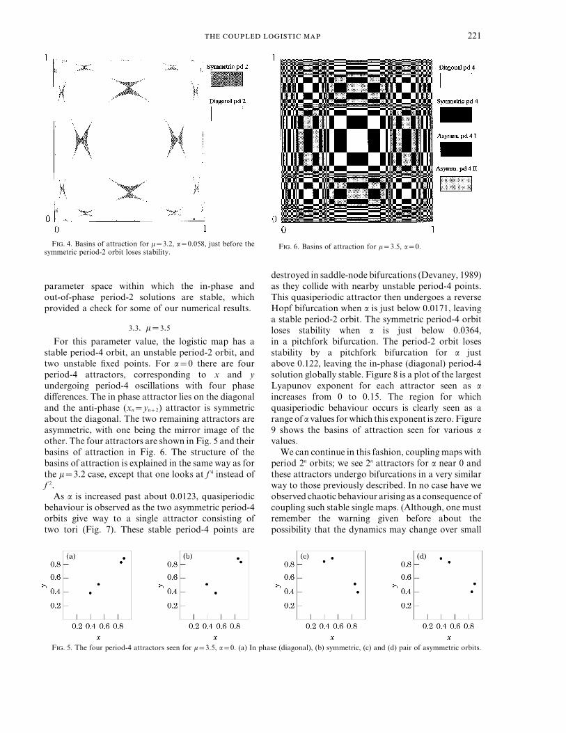
For this parameter value, the logistic map has astable period-4 orbit, an unstable period-2 orbit, andtwo unstable fixed points. For a=0 there are fourperiod-4 attractors, corresponding to x and yundergoing period-4 oscillations with four phasedifferences. The in phase attractor lies on the diagonaland the anti-phase (xn=yn+2) attractor is symmetricabout the diagonal. The two remaining attractors areasymmetric, with one being the mirror image of theother. The four attractors are shown in Fig. 5 and theirbasins of attraction in Fig. 6. The structure of thebasins of attraction is explained in the same way as forthe m=3.2 case, except that one looks at f 4 instead off 2.

As a is increased past about 0.0123, quasiperiodicbehaviour is observed as the two asymmetric period-4orbits give way to a single attractor consisting oftwo tori (Fig. 7). These stable period-4 points are

F. 5. The four period-4 attractors seen for m=3.5, a=0. (a) In phase (diagonal), (b) symmetric, (c) and (d) pair of asymmetric orbits.

. . 222

F. 7. Two-torus attractor seen for m=3.5, a=0.015.

is increased the attractor undergoes a complicatedsequence of changes. Many intervals of a values giveperiodic behaviour, as is seen in the single logistic mapbeyond the onset of chaos. As a result of this,a numerical study of the systemwill tend tomiss a lot ofperiodic behaviour. Before discussing these periodicwindows,weconsider themainchanges that the chaoticattractor undergoes as the coupling is increased.

As a is increased between 0.0130 and 0.0135,the single block chaotic attractor suddenly changesinto a two block attractor. A qualitative change in thestructure of the chaotic attractors has occurred, sucha change is known as a crisis. This type of crisis is calledan interior crisis (Grebogi et al., 1982, 1983; Sakaguchi& Tomita, 1987), and it is most easily understood byconsidering the attractors changing with decreasing a.As a decreases, the two blocks of the attractor growand move closer together. At the crisis, the blockscollide with an unstable fixed point on the basinboundary (in this case the unstable point is (x*, x*), onthe diagonal). Points which come near enough to theunstable point are then thrown out into the new partof the attractor. The point then wanders around thenew part of the attractor for a while before returningto the part of the attractor which existed before. As aresult, in the neighbourhood of the crisis very longintermittent behaviour is observed, with the pointwandering around the two parts of the chaotic set forperiods of time with sudden jumps between the two.Figure 10 shows the chaotic attractors in the vicinityof the crisis.

As a is increased between 0.041 and 0.042,we observe another crisis. The symmetric two-block

intervals of parameters or that attractors may becreated with very small basins of attraction.)

We now turn our attention to the situation when theindividual maps are chaotic. We couple maps whosechaotic attractors have 2n band structure, that isthe attractor is contained within 2n sub-intervals of[0, 1] which are invariant under f 2n and are permutedby f.

3.4. m=3.7

The logistic map exhibits one band chaos for thisparameter value. When the maps are coupled witha=0 we see just one attractor, which is squareand symmetric about the diagonal. As the coupling

F. 8. Plot of largest Lyapunov exponent (l) vs a for each of the attractors seen for m=3.5. Quasiperiodic behaviour is seen when l=0.The pitchfork bifurcations are seen to occur as l becomes zero and the curves end.

223

F. 9. Basins of attraction for m=3.5. (a) a=0.035, just before thesymmetric period-4 orbit is lost. (b) a=0.12, just before the period-2orbit becomes unstable.

periods 2n are seen for ne2, the final resultof this cascade being a pair of asymmetric period-4orbits. These orbits can be seen, for instance, whena=0.056.

These period-4 orbits are destroyed in saddle nodebifurcations just below a=0.05614. The attractorformed appears to be made up of two tori which arevery wavy near to where the periodic points used to be.Such an attractor has been observed in other studies ofcoupled maps (Hogg & Huberman, 1984; Kaneko,1984), and its structure is studied in detail by Kaneko(1984). The motion on this attractor appears to bechaotic just above the bifurcation point (although thischaos is punctuated by periodic windows). As thecoupling is increased, the waves become straightenedand the motion becomes quasiperiodic (Fig. 11.). Thisattractor undergoes a reverse Hopf bifurcation whena is between 0.0746 and 0.0747, giving rise to a period-2orbit. The orbit becomes unstable just below 0.155 ina pitchfork bifurcation. These last two bifurcations,involving period-2 orbits, occur just as predicted by theanalytic results of Gyllenberg et al. (1993).

One example of a periodic window occurs when0.0413QaQ0.0418, when a period-12 window is seen.The window begins as a crisis turns the symmetrictwo-block chaotic attractor into a pair of asymmetric12-piece attractors. These attractors undergo a cascadeof further crises giving rise to 24, 48, and 96 pieces, andso on. These crises accumulate at a certain a value,which is the accumulation of a reverse period-doublingcascade that follows. This cascade ends with a pair ofasymmetric period-12 orbits. Towards the end of thewindow, long chaotic transients are seen before thesystem settles down to periodic behaviour. Theperiodic behaviour ends as the two stable period-12orbits collide with and destroy two unstable period-12orbits in two simultaneous saddle node bifurcations. Abifurcation diagram for one of the attractors duringthe window is shown in Fig. 12. (We plot 20000 xn

values for each a value, after allowing transients to dieout. When these are plotted on a scale from 0 to 1, theyare seen to cluster around 12 x values. Figure 12 is amagnification of one of these clusters. The initialcondition is chosen so that the same attractor of thepair is explored each time.) Notice the self-similaritythat is seen in this system; the bifurcation structurewithin the window is very similar to the mainbifurcation sequence described above with crises andreverse period doublings. Within the figure, we seeperiodic windows which follow bifurcation sequencessimilar to that of the whole figure. Just beyond the endof the periodic window we observe intermittentbehaviour (Schuster, 1989). The iterates move veryslowly when they come near to where the fixed points

attractor splits into a pair of asymmetric four pieceattractors. This is known as an attractor merging crisis(Ott, 1993). Intermittent behaviour is again observedjust before the crisis (for example at a=0.0419) withiterates behaving almost as if there were two separateattractors. The iterates are seen to move aroundone-half of the attractor before being thrown onto theother half, where they move around for a while beforereturning to the first half.

A cascade of crises occurs as a is increased further,resulting in a pair of asymmetric period 2n piece chaoticattractors being seen. (For instance, eight pieces areseen when a=0.048, 16 when a=0.0484.) These crisesaccumulate just below 0.0486, which is also theaccumulation point of a cascade of reverse perioddoublings which then follows. Periodic orbits of

. . 224

F. 10. Chaotic attractors in vicinity of the crisis, m=3.7. (a) Diagonal block attractor seen for a=0.012. (b) Symmetric two-block attractorseen for a=0.0135.

used to be, and during these episodes the dynamics arenearly periodic. Once the iterate has left this region themotion becomes chaotic until the iterate comes closeto the region again. Over a long period of timewe observe nearly periodic dynamics punctuated byepisodes of chaotic behaviour.

For some a values within this bifurcation sequencewe see the creation of new attractors. For instance, justabove 0.0913 we see the creation of a chaotic attractor.This attractor then undergoes various bifurcationsgoing from chaos to torus to a period-4 orbit, withvarious periodic orbits interrupting this sequence.The period-4 orbit disappears just below 0.1269 ina pitchfork bifurcation. This procees is repeated inthe interval (0.1012, 0.1037). Figure 13 shows thebasins of attraction of the various attractors seenwhen a=0.1018. (Points that start on the diagonalwill remain on the diagonal, undergoing chaotic

dynamics, even though the in phase set is not attractingin this case. We do not show this behaviour on thebasins of attraction plot since there are pointsarbitrarily close which tend to one of the attractingsets.)

For large values of the coupling, the only attractingset is an in-phase chaotic attractor, with both x and ybehaving as a single logistic map with m=3.7. Thein-phase chaotic set becomes an attractor as its smallerLyapunov exponent becomes negative when a isbetween 0.149 and 0.150. Below this a value asymmetric chaotic set is seen, although thismaybe verylong transient behaviour. For some a values below0.149 the in-phase set appears to be an attractor eventhough the smaller Lyapunov exponent is positive,corresponding to points of the diagonal moving awayexponentially on average. We believe this is anumerical effect caused by the finite precision of the

F. 11. Magnification of one of the two tori seen for m=3.7. (a) Wavy tori, a=0.0574. (b) a=0.604, notice the torus is less wavy (c) a=0.674,when the tori have lost the waves.

225

F. 12. Bifurcation structure observed during a periodic window when m=3.7. This figure is a magnification about one of the 12 clustersof xn values seen. At the extreme left of the figure we see the crisis which gives rise to the window. A cascade of reverse crises follows, interruptedby further periodic windows. Further right, a reverse period-doubling cascade can be seen. The window ends with a saddle node bifurcationat the right of the figure.

computer arithmetic. If the iterate (xn , yn ) comes closeenough to the diagonal then the computer may setxn=yn and all future iterates will then stay on thediagonal. After the loss of the stable period two orbitnear 0.155, almost all initial conditions are attracted tothe in-phase chaotic attractor.

3.5. m=3.65

The individual maps show two-band chaos, forno coupling we see two attractors; one consists oftwo square blocks centred on the diagonal, and theother is a symmetric pair of rectangular blocks. Asthe coupling is increased, both of these attractorsundergo bifurcation sequences which are extremelysimilar to that seen in the m=3.7 case. For this reasonwe shall not give as much detail in describing thesesequences, instead we shall give an a value when eachdifferent attractor described can be seen. (We do notgive the a values of the bifurcation points.)

The symmetric two-block attractor undergoes acrisis, giving rise to a pair of asymmetric four-blockchaotic attractors (these new attractors can be seen, forinstance, when a=0.025). Later, these attractorsundergo a cascade of crises followed by a reverseperiod-doubling cascade which ends up with a pair

of asymmetric period-4 orbits (a=0.042). Theseare destroyed in saddle node bifurcations, leaving atwo-torus attractor with quasiperiodic dynamics(a=0.047). In this casewe do not see chaotic behaviourbetween the loss of the periodic orbits and thequasiperiodic behaviour (although it could

F. 13. Basins of attraction for m=3.7, a=0.1018. Notice theparticularly detailed self-similar structure.

. . 226

F. 14. Basins of attraction for m=3.65, a=0.045.

of asymmetric period-4 orbits which resulted from thesymmetric two-block attractor.

As in the m=3.7 case, attractors are created whichundergo similar bifurcation sequences before beingdestroyed. One example of this occurs within theinterval (0.070, 0.073). Figure 15 shows the basinsof attraction for a=0.070875, when a period-2 orbit(the product of the symmetric two block), a four-torusattractor (the product of the diagonal two block) anda period-36 orbit (a product of the new attractor)coexist.

For large values of the coupling, the only attractingset is an in-phase chaotic attractor, with both x and ybehaving as a single logistic map with m=3.65.The second Lyapunov exponent of the in phase setbecomes negative when a is near 0.113. After the lossof the stable period two orbit near 0.147, almost allinitial conditions are attracted to the in-phase chaoticattractor.

We have repeated these calculations for other m

values for which the logistic map shows 2n band chaos.Similar bifurcation sequences are observed, with chaosgoing to quasiperiodicity, then to periodic behaviour.The in phase attractor is always favoured by largevalues of the coupling, with both x and y behaving likeiterates of the single logistic map at the same m value.

4. The Effects of Linear Coupling

In this section we discuss how the results seen aboveare changed if we employ a linear coupling, as ineqns (2). This form of coupling may be considered as adiscrete space analogue of the Laplacian (92) couplingused in reaction-diffusion equations. The linear

occur over a very small parameter range). A reverseHopf bifurcation causes the attractor to become aperiod-2 orbit (a=0.06). This orbit loses stability in apitchfork bifurcation near 0.147.

The ‘‘diagonal’’ two block attractor undergoes asimilar bifurcation sequence. The attractor becomes asymmetric four-block attractor in a crisis (a=0.057).A complicated bifurcation sequence follows whichresults in a quasiperiodic four-torus attractor beingseen (a=0.07). Later this becomes a symmetricperiod-4 orbit in a reverse Hopf bifurcation (a=0.075). The period-4 orbit finally loses stability ina pitchfork bifurcation when a is near 0.109.Once again, periodic windows are seen within thisbifurcation sequence.

Periodic windows are seen throughout thechaotic parameter regions. For instance, we seethat the symmetric four-piece attractor has a largeperiodic window within the interval (0.062, 0.064).Within this window, in addition to period doublingsand crises, we see the multiple Hopf bifurcationscharacteristic of the quasiperiodic route to chaos (seeAppendix). For a=0.06248, we see a period-44(=4×11) orbit, and as we decrease a a Hopfbifurcation occurs leaving 44 tori (for instance whena=0.0624). As a is decreased further we see aperiod-308 (=44×7) orbit (a=0.06212) whichundergoes a further Hopf bifurcation, giving rise to a308-torus attractor (a= 0.06209). As a is decreasedfurther, the tori break up and the dynamics becomechaotic.

Figure 14 shows the basins of attraction seen fora=0.045, when the chaotic attractor which is theproduct of the diagonal two-block coexists with a pair F. 15. Basins of attraction for m=3.65, a=0.070875.

227

F. 16. Structure of attractors for m=2.9 with linear coupling. (a) Two tori, a=0.27; (b) frequency locking (period 10), a=0.29; (c) one ofthe asymmetric pair of 16 tori, a=0.326; (d) chaos, a=0.3314.

coupling is also mathematically convenient as it doesnot introduce any extra nonlinear terms into theequations. The coupling is not biologically realistic,however, and it does cause some unexpected behaviourto occur.

One example of this unexpected behaviour occurswhen we couple two logistic maps with m=2.9 usinglinear coupling. For this parameter value, as discussedpreviously, the logistic map has two fixed points; onestable (x*=(m−1)/m) and one unstable (m=0).For a $ [0, 0.05] almost all points are attracted to(x*, x*). At a=0.05 this point becomes unstable as itundergoes a period doubling bifurcation, creating astable period-2 attractor that is symmetric in (x, y):{(x1, y1), (y1, x1)}.

As a increases further, the period-2 attractorundergoes a Hopf bifurcation (at a just below 0.268),producing two symmetric tori. These tori undergo acomplex sequence of bifurcations, including furtherfrequency lockings and Hopf bifurcations. Oneexample of frequency locking is seen between about0.289 and 0.298 when a period-10 orbit is seen.An asymmetric pair of period-16 orbits can be seenwhen a=0.325; these undergo Hopf bifurcations,producing an asymmetric pair of 16 tori which canbe seen, for instance, when a=0.3256. Chaoticbehaviour is seen as a is increased, for instance whena=0.3314. Periodic windows are seen beyond this a

value, as they are in the single logistic map beyondthe onset of chaos. Figure 16 shows some of the

. . 228

attractors seen for this value of m as a varies. Multipleattractors are seen for this value ofm, for examplewhena=0.325 a two-torus attractor coexists with theperiod-16 orbits described above. This is in contrast tothe nonlinear coupling of the two maps at this m value,when only one attractor was ever seen.

The coupling is seen to destabilize individually stablemaps, producing chaotic behaviour. We also observethat the in-phase attractor is no longer favoured bylarge couplings. Similar behaviour is observed forother m values for which the logistic map exhibits stableperiodic behaviour. This counterintuitive behaviour ispurely a consequence of the incorrect coupling of thetwo maps.

When two chaotic logistic maps are coupled inthis fashion, we again see that the coupling can lead tostable behaviour. Bifurcation sequences similarto those described for nonlinear coupling are seen.As for the periodic maps, large coupling no longerfavours the in-phase attractor.

The dangers of coupling discrete time maps withlinear coupling terms have been noted before. Kot &Schaffer (1986) developed integrodifference equationsto model growth and dispersal, and used nonlinearcouplings. In their paper they note that linearcouplings mix generations and may lead to counter-intuitive results. Jackson (1990) considers couplingmaps in a more general context, and warns thatthe diffusive process must be kept separate from thereproductive process in order to keep in touch with‘‘reality’’.

5. Discussion

The model shows many interesting types ofbehaviour which may be important when consideringthe dynamics of real populations. The most importantresult is that the scale on which measurements of thepopulation is taken is crucial, and that information onthe distribution of the population is also necessary tounderstand the dynamics. A similar result was foundby Sugihara et al. (1990) when analysing the monthlyincidence of measles in England and Wales. On acity-by-city scale they found evidence of low-dimensional chaos, whereas on a country-wide scalethe dynamics appeared to be a two-year noisycycle. Coupling can stabilize individually chaoticsubpopulations to give stable dynamics of thepopulation as a whole. The reverse is also seen withquasiperiodic dynamics resulting from the coupling oftwo populations that individually show identicalperiodic behaviour.

We may ask what sort of dynamic behaviours arepreferable for thepopulationasawhole topersist. Ithas

beensuggestedthatchaoticbehaviourofthepopulationas a whole may increase the probability of extinctionbecause (for many chaotic systems) there is a highprobability that the population density will eventuallygo below an extinction threshold (Berryman &Millstein, 1989). If the population is patchy this wouldnot necessarily be the case, unless the populationsin different patches were synchronized. In this system,strongcouplingbetweenpatcheswill lead to thembeingsynchronized even if they were individually chaotic.However, if the populations in different patches werenot synchronized, then diffusion between patcheswould be able to counteract local extinctions. Similarresults have been seen in simulations where couplinglarge arrays of chaotic Rossler attractors gave rise tostable spiral patterns which could withstand theobliteration of large parts of the spiral (Klevecz et al.,1991). In weakly coupled systems it has been suggestedthat chaos can amplify local population noise, leadingto a greater degree of asynchrony between localpopulations (Allen et al., 1993).

The existence of multiple attractors means thatpopulations can exhibit very different dynamicbehaviours, even if per capita birth and death rates anddiffusion rates are the same. It is possible that a suddenchange in the populations due to some external causecan move the system between these differ-ent behaviours, in some cases from stable to chaoticdynamics. If an attractor is close to the edge of its basinof attraction then only a small perturbation(for instance small amplitude random noise) maybe necessary to switch the system from one sort ofbehaviour to another.

If the parameters of the model are allowed tovary with time there can be dramatic changes inthe population dynamics. The crises and periodicwindows that were seen represent dramatic changes inthe behaviour for very small changes in the parameters.In the vicinity of these changes, long episodes ofintermittent and transient behaviours are seen.Populations may exhibit apparently periodic be-haviour for long periods of time and then suddenlyundergo chaotic bursts before returning to almostperiodic behaviour. This means that if a population isobserved over a short period of time then theinteresting part of the dynamics may be missed, sincefor most of the time the dynamics appear tame.

The multiple attractors pose a trap for the unwarynumerical experimenter. One method that has beenused to study eqns (2) is to fix one initial point andconsider iterates for deferent values of the coupling andbifurcation parameters. Whilst this is fine for the singlelogistic map (which has just one attracting set), this willnot do here. As parameters change so the basins of

229

attraction grow and shrink, our one initial point mayfind itself in a different basin and a change in behaviourwill be observed. This change in behaviour is dueentirely to the multiple attractors and not to somechange in the dynamics of the map. Many authors havefallen into this trap; for instance Ferretti & Rahman(1988) studied the map numerically by iterating thesingle initial condition (0.5, 0.5).

6. Conclusions

The coupled logistic map exhibits a much widerrange of dynamic behaviour than the single logisticmap, much of which may be important to the study ofpopulation dynamics. Intermittent behaviour maylead to populations behaving almost periodicallyfor long periods of time but with short bursts ofapparently random behaviour. Crisis behaviour maybe more dramatic, with sudden changes in dynamicbehaviour occurring for small changes in theparameters controlling the nature of the dynamics.The spatial nature of the problem is seen to beimportant, with the coupling able to cause individuallystable periodic populations to undergo quasiperiodicdynamics, or able to stabilize individually chaoticpopulations. More realistic models would includebetter descriptions of the local dynamics (although forsimple models one tends to see similar typesof dynamics) and of the spatial degrees of freedom.Thelatter would require the consideration of more patchesand a more detailed description of movement betweenpatches. Inhomogeneities in the environment could beconsidered by varying the coupling and bifurcationparameters across the lattice.

This work was supported by the Wellcome Trust(Biomathematical Scholarship, grant number 036134/Z/92/Z). I wish to thank R. M. May for discussions andencouragement. I also wish to thank two anonymous refereeswhose helpful criticisms and thoughtful comments on theoriginal manuscript led to major improvements in this work.

REFERENCES

A, J. C. (1975). Mathematical models of species interactionsin time and space. Am. Nat. 109, 319–342.

A, J. C., S, W. M. & R, D. (1993). Chaos reducesspecies extinction by amplifying local population noise. Nature,Lond. 364, 229–232.

B, A. A. & M, J. A. (1989). Are ecological systemschaotic—and if not, why not? TREE 4, 26–28.

C, H. N., H, M. P. & M, R. M. (1992). The spatialdynamics of host-parasitoid systems. J. Anim. Ecol. 61, 735–748.

C, P. H. (1981). Dispersal and the stability of predator-preyinteractions. Am. Nat. 118, 673–701.

C, J.&Y, J.A. (1978). A transition from Hopf bifurcationto chaos: computer experimentswithmaps inR2. In:TheStructureof Attractors in Dynamical Systems. Berlin: Springer-Verlag.

D, R. L. (1989). An Introduction to Chaotic DynamicalSystems. Redwood City, CA.: Addison Wesley.

E, J.-P. & R, D. (1985). Ergodic theory of chaos andstrange attractors. Rev. Mod. Phys. 57, 617–656.

F, A. & R, N. K. (1988). A study of coupled logisticmap and its applications in chemical physics. Chem. Phys. 119,

275–288.G, C., O, E. & Y, J. A. (1982). Chaotic attractors in

crisis. Phys. Rev. Lett. 48, 1507–1510.G, C., O, E. & Y, J. A. (1983). Crises, sudden changes

in chaotic attractors, and transient chaos. Physica D 7, 181–200.G, M., S, G. & E, S. (1993). Does

migration stabilize local population dynamics? Analysis of adiscrete metapopulation model. Math. BioSci. 118, 25–49.

H, M. P., C, H. N. & M, R. M. (1991). Spatialstructure and chaos in insect population dynamics. Nature, Lond.353, 255–258.

H, A. (1993). Complex interactions between dispersal anddynamics: lessons from coupled logistic equations. Ecology 74,

1362–1372.H, T. & H, B. A. (1984). Generic behavior of coupled

oscillators. Phys. Rev. A 29, 275–281.J, E. A. (1990). Perspectives of Nonlinear Dynamics, Vol. 2.

Cambridge: Cambridge University Press.K,K. (1983). Transition from torus to chaos accompanied by

frequency lockings with symmetry breaking. Prog. Theor. Phys.69, 1427–1442.

K, K. (1984). Oscillation and doubling of torus. Prog. Theor.Phys. 72, 202–215.

K, R. R., P, J. & B, J. (1991). Autogenousformation of spiral waves by coupled chaotic attractors.Chronobiology Intl. 8, 6–13.

K, M. (1989). Diffusion-driven period-doubling bifurcations.BioSystems 22, 279–287.

K, M. & S, W. M. (1986). Discrete-time growth-dispersalmodels. Math. BioSci. 80, 109–136.

M, R. M. (1976). Simple mathematical models with verycomplicated dynamics. Nature, Lond. 261, 459–467.

N, S., R, D. & T, F. (1978). Occurence ofstrange axiom-A attractors near quasiperiodic flow on Tm, me3.Commun. Math. Phys. 64, 35–40.

O,E. (1993).Chaos inDynamical Systems. Cambridge:CambridgeUniversity Press.

P, M. (1993). Diffusion-induced chaos in a spatialpredator-prey system. Proc. R. Soc. Lond. B 251, 1–7.

R, J. D. (1988). Environmental variability, migration andpersistence in host-parasitoid systems. Am. Nat. 132, 810–836.

R, D. & T, F. (1971). On the nature of turbulence.Commun. Math. Phys. 20, 167–192.

S, H. & T, K. (1987). Bifurcations of the coupledlogistic map. Prog. Theor. Phys. 78, 305–315.

S, K. & A, T. (1990a). Numerical study on acoupled-logistic map as a simple model for a predator-preysystem. J. Phys. Soc. Jpn. 59, 1184–1198.

S, K. & A, T. (1990b). Self-similar structures in the phasediagram of a coupled-logistic map. J. Phys. Soc. Jpn. 59,

1123–1126.S, H. G. (1989). Deterministic Chaos, An Introduction, 2nd

revised edn. Weinheim: Physik-Verlag.S, G., G, B. & M, R. M. (1990). Distinguishing

error from chaos in ecological time series. Phil. Trans. R. Soc.Lond. B 330, 235–251.

APPENDIX

The Hopf Bifurcation and Quasiperiodicity

For most sets of parameter values, altering themslightly does not change the qualitative behaviourof the system. The changes in qualitative behaviour are

. . 230

known as bifurcations and the parameter valuesat which they occur are called bifurcation points. Somebifurcations only affect the dynamics in a smallneighbourhood; these are called local bifurcations.Such bifurcations are associated with one or more ofthe eigenvalues of the Jacobian matrix Df havingmodulus one. (This is for a fixed point; for periodn orbits one considers the product Jacobian Df n.)Two simple bifurcations which are observed in oursystem are saddle node (where a pair of fixed points off n are produced, one stable and one unstable)andperiod doubling (where a stable period norbit losesits stability and a stable period 2n orbit is created),these are both seen in the logistic map. The seconddimension allows other bifurcations to occur,including the Hopf bifurcation.

The Hopf bifurcation occurs when a complexconjugate pair of eigenvalues crosses the unitcircle (if there is a complex eigenvalue a+ib thenits complex conjugate a−ib is also an eigenvalueas the Jacobian matrix is real). At this point afixed point undergoes a change in stability and aninvariant curve is created. This is most easily seenin a simple example. Consider the followingtwo-dimensional map

F0xy1={l−(x2+y2)}0cos a −sin a

sin a cos a10xy1,

where a is fixed and l is a parameter.The origin is always a fixed point and the Jacobian

has eigenvalues l(cos a+i sin a), both have modulus=l = so they cross the unit circle as l increases through

one. If we change to polar co-ordinates (r, u) the mapbecomes

rn+1=lrn−r3n

un+1=un+a

For −1QlQ1 the origin is a stable fixed point, butas l passes through one the origin loses its stability. Atthe bifurcation point an invariant circle, r=zl−1, iscreated which attracts nearby points. The dynamics onthe circle are given by

un+1=un+a.

If a is a rational multiple of 2p, a=(p/q)2p, thenthe orbit will be periodic with period q. If a is anirrational multiple of p then the orbit will not close up.This is called a quasiperiodic orbit.

More generally, a Hopf bifurcation gives rise toan invariant closed curve topologically equivalent toa circle, and the dynamics of the map on thiscurve can be more complicated than a simplerotation. Higher iterates of the map may undergoHopf bifurcations, for instance a period n orbit maygive rise to quasiperiodic behaviour on n tori. Asthe parameter varies, it is possible for more than oneHopf bifurcation to occur. Such Hopf bifurcations areinvolved in the various quasiperiodic routes to chaoswhich have been proposed (Ruelle & Takens, 1971;Newhouse et al., 1978; Curry & Yorke, 1978). Theseroutes to chaos have many universal properties, whichhave been studied extensively (see Schuster, 1989, foran excellent summary of these). For instance, onefeature that is often observed is frequency locking,where the system exhibits periodic behaviour for quitelarge windows of parameter values.