THE COOPER UNION ALBERT NERKEN SCHOOL OF ENGINEERING THE USE AND
153
THE COOPER UNION ALBERT NERKEN SCHOOL OF ENGINEERING THE USE AND OPTIMIZATION OF THE HELIX SHAPE AS THE PRIMARY STRUCTURAL ELEMENT IN THE DESIGN OF A STEEL BRIDGE by Jason Damiano A thesis submitted in partial fulfillment of the requirements for the degree of Master of Engineering April 13, 2012 Prof. Cosmas Tzavelis Advisor
Transcript of THE COOPER UNION ALBERT NERKEN SCHOOL OF ENGINEERING THE USE AND

THE COOPER UNION
ALBERT NERKEN SCHOOL OF ENGINEERING
THE USE AND OPTIMIZATION OF THE
HELIX SHAPE AS THE PRIMARY STRUCTURAL ELEMENT
IN THE DESIGN OF A STEEL BRIDGE
by
Jason
Damiano
A thesis submitted in partial fulfillment
of the requirements for the degree of
Master of Engineering
April 13, 2012
Prof. Cosmas Tzavelis
Advisor

1
THE COOPER UNION FOR THE ADVANCEMENT OF SCIENCE AND ART
ALBERT NERKEN SCHOOL OF ENGINEERING
This thesis was prepared under the direction of the Candidate's Thesis Advisor and has
received approval. It was submitted to the Dean of the School of Engineering and the full
Faculty, and was approved as partial fulfillment of the requirements for the degree of
Master of Engineering.
__________________________________
Dean, School of Engineering - Date
________________________________
Prof. Cosmas Tzavelis – April 13, 2012

2
i. Acknowledgement
I would first like to thank my advisor, Professor Cosmas Tzavelis. His guidance
and support were vital in the process of creating this thesis. His knowledge and expertise
in the design of bridges was extremely important throughout this process, and his help
was greatly appreciated.
I would also like to thank the rest of the Civil Engineering Department,
specifically Professor Jameel Ahmad, Professor Vito Guido, Professor Joseph Cataldo
and Professor Constantine Yapijakis. I would like to express my gratitude for their
support in choosing me as a candidate for the Masters Program.
Next, I would like to thank Dr. Simon Ben-Avi and the rest of the Cooper Union
administrative staff. Without their work, the school would not move forward in the way
it does.
I would also like to thank Dean Stephen Baker, whose help, support and guidance
in my years at The Cooper Union made my experience significantly more enjoyable.
Next, I would like to thank my friends, who have made the entire experience at
the Cooper Union so much more memorable. My time spent at The Cooper Union was
always positive because of them.
Finally, and most importantly, I would like to thank my family. My mom, dad
and sister have supported me throughout my years at The Cooper Union, and without
them, this would not have been possible.

3
ii. Abstract
The helix shape is an aesthetically pleasing one that has rarely been used in
structural design. This study contains a complete analysis on the use of the helix shape in
the design of a steel bridge with a span length of 2000 feet. The 2000 foot span is longer
than that of any other steel non-suspension or cable stayed bridge in the world. The
initial trials find the weaknesses in the helix shape, which are the lack of support for the
members as they circle about the deck, and this causes excessive deflections, and the
other flaw being the excessive thinness of the design near the supports, making it
extremely susceptible to shear. An alternative design solution that contains the aesthetic
beauty of the helical curve along with the satisfying the structural strength needs is found
and recommended. The solution is to combine a “full-helix” shape with that of the “half-
helix”, which provides the necessary support and aesthetic qualities that were initially set
out to be studied and optimized. The final design passes all necessary code standards that
are tested for in the design program during the analysis.

4
iii. Table of Contents
Acknowledgment i
Abstract ii
Table of Contents iii
List of Figures and Tables iv
Table of Nomenclature v
1. Introduction 1
1.1 Statement of Problem 2
1.2 Designing Bridges for Aesthetics:
Robert Maillart and Santiago Calatrava 3
2. Structural Background Information 23
2.1 The Simply Supported Beam 24
2.2 Commonly Used Equations in Bridge Design 26
2.3 The Double Helix Shape 29
3. Autodesk Robot Structural Analysis 30
3.1 Modeling a Helix Shaped Bridge in Robot 31
4. Optimizing the Helix Bridge Structure for Live Load Deflections 46
4.1 Radius Size Optimization 49
4.2 Deck Thickness Optimization 57
5. Optimizing the Helix Bridge Structure for Dead Load Deflections 60
5.1 Deck Diagonal Optimization 63
5.2 Layered Helix Optimization 65
5.3 The Use of a Sloped Deck 74

5
5.4 Bracing the Helix Structure to Reduce Dead Load Deflections 78
6.0 Optimizing the Individual Steel Members 84
6.1 Optimizing the Member Sections 86
6.2 Failure in the Second Order Analysis 90
7.0 Optimizing Alternative Designs to Pass Second and Third Order
Analyses 93
7.1 Alternative Design: The Double Helix 94
8.0 Conclusions and Recommendations 101
Appendices 102 111
Bibliography 105

6
iv. List of Figures and Tables
List of Figures:
Figure 1.2.1 – The Staffacher Bridge 5
Figure 1.2.2 – The Stauffacher Bridge’s three hinges 6
Figure 1.2.3 – Cross-section of the Zuoz Bridge 6
Figure 1.2.4 – A photograph of The Zuoz Bridge 7
Figure 1.2.5 – Cross-section of the bridge over the Rhine River at Tavanasa 8
Figure 1.2.6 – Maillart’s drawings of the bridge over the Rhine River at
Tavanasa 8
Figure 1.2.7 – A drawing of the Valtscheilbach Bridge 9
Figure 1.2.8 – A photo graph of the Valtscheilbach Bridge 9
Figure 1.2.9 – A drawing of the Chatelard 10
Figure 1.2.10 – A photograph of the Chatelard 11
Figure 1.2.11 – The bridge over the Grand Fey Viaduct 12
Figure 1.2.12 – A photograph of the Salginatobel Bridge 13
Figure 1.2.13 – A model of the Walenesse Bridge 14
Figure 1.2.14 – A model of the Cabelleros Footbridge 15
Figure 1.2.15 – A model of the Cabelleros Footbridge (alternate view) 16
Figure 1.2.16 – A photograph of the Bach de Roda Bridge 17
Figure 1.2.17 – A photograph of the Oudry-Mesly Footbridge 18
Figure 1.2.18 – A photograph of the Alamillo Bridge 19
Figure 1.2.19 – A photograph of the Trinity Footbridge 20
Figure 1.2.20 – A photograph of The Lyre 21
Figure 1.3.1 – The Helix Bridge in Singapore 23
Figure 1.4.1 – The Chaotianmen Bridge 26
Figure 1.4.2 – The Lupu Bridge 27
Figure 1.4.3 – The Pont de Quebec 28
Figure 2.1.1 – Moment and shear diagrams in a simply supported beam
Figure 2.1.2 – Stress distribution in a beam
Figure 3.1.1 – The “Load Types” window
Figure 3.1.2 – The “New Section” window
Figure 3.1.3 – The “Bars” windows
Figure 3.1.4 – Helix quarter-circle cross-section
Figure 3.1.5 – The “Translation” window
Figure 3.1.6 – Cross-section of the quarter helix with deck connections
Figure 3.1.7 - Cross-section of the quarter helix with deck connections
Figure 3.1.8 – Cross-sections after the horizontal and vertical mirrors
Figure 3.1.9 – Isometric view of half of the helix bridge
Figure 3.1.10 – The “Rotation” window
Figure 3.1.11 – Isometric view showing the pinned end supports, cladding
and live load.
Figure 3.1.12 Isometric view showing the completed model.
7
Figure 3.2.1 – The “Results” drop-down list 52
Figure 3.2.2 – Side-view of the live load deflected shape 53
Figure 3.2.3 – The “Analysis Type” window 54
Figure 3.2.4 – The “Nonlinear Analysis Parameters” window 55
Figure 3.2.5 – Non-linear analysis failure notifications 56
Figure 3.2.6 – The steel member design “Calculations” window 57
Figure 3.2.7 – The final steel member design “Calculations” window 58
Figure 3.2.8 – Steel member calculation results for the first order dead load case 59
Figure 4.0.1 – Cross section in the X-Z plane with a 65 foot radius.
Figure 4.0.2 – Isometric view.
Figure 4.0.3 – Side view in the Y-Z plane with a 2000 foot length
Figure 4.0.4 – Side view of the exaggerated deflected shape in the Y-Z plane.
Figure 4.1.1 – Cross-sections of the best performing radius optimization designs.
Figure 4.1.2 – Maximum live load deflections for 65 foot width models of
varying height 52
Figure 4.1.3 – Maximum dead load deflections for 65 foot width models of
varying height 53
Figure 4.1.4 – The exaggerated deflected dead load shape of the cross-
section of the 65 by 130 foot radius model. 54
Figure 4.1.5 – The exaggerated deflected dead load shape of the side-view
of the 65 by 130 foot radius model. 55
Figure 4.1.6 – The exaggerated deflected dead load shape of the isometric
view of the 65 by 130 foot radius model. 55
Figure 4.2.1 – Helix bridge model cross-sections with decks. 58
Figure 4.2.1 – Helix bridge model side-views with decks. 59
Figure 5.0.1 – Cross-section of the 65 by 130 foot radius model with the
compression helix highlighted in red. 61
Figure 5.0.2 – Isometric view of the 65 by 130 foot radius model with the
compression helix highlighted in red. 61
Figure 5.1.1 – Deck diagonal variations listed from top to bottom 64
Figure 5.2.1 – Cross-section of the 100 by 100 foot model with no inner helix
layers and a ½ inner helix layer. 68
Figure 5.2.2 – Cross-section of the 100 by 100 foot model with ½ & ¾ inner
helix layers and ¼, ½ & ¾ inner helix layers. 68
Figure 5.2.5 – Side views of the 100 by 100 foot models, listed from top 69
Figure 5.2.4 – Cross-section of the 65 by 130 foot model with no inner helix
layers and a ¾ inner helix layer. 70
Figure 5.2.5 – Cross-section of the 65 by 130 foot model with ¾ & ⅞ inner
helix layers and ⅜, ¾ & ⅞ inner helix layers. 70
Figure 5.2.6 – Side views of the 65 by 130 foot models, listed from top 71
Figure 5.2.7 – Exaggerated deflected cross-section of 65 by 130 foot model
with ¾ and ⅞ inner helix layers. 72
Figure 5.2.8 – Exaggerated deflected side view of the 65 by 130 foot model
with ¾ and ⅞ inner helix layers. 73
Figure 5.3.1 – Cross-section of the 65 by 130 foot radius model with the

8
sloped deck. 75
Figure 5.3.2 – Side view of the 65 by 130 foot radius model with the sloped deck 75
Figure 5.3.3 – Cross-section of the 100 by 100 foot radius model with the sloped
deck. 76
Figure 5.3.4 – Cross-section of the 100 by 100 foot radius model with the sloped
deck 76
Figure 5.4.1 – Exaggerated deflected shape of sections 8 through 18 of the
100 by 100 foot radius model 77
Figure 5.4.2 – Various bracing types, listed from top left to bottom right 79
Figure 5.4.3 – Cross-sections of the 65 by 130 foot models with top &
bottom bracing and center deck bracing. 81
Figure 5.4.4 – Cross-sections of the 100 by 100 foot models with top &
bottom bracing (left) and center deck bracing (right). 81
Figure 5.4.5- Isometric view of the most efficient helix bridge shape with
bracing. 83
Figure 6.1.1 – The member with the lowest axial force 85
Figure 6.1.2 – The members with the highest axial forces 85
Figure 6.2.1 – Cross-section of the exaggerated deflected shape that passes
the first order analysis, but fails the second order analysis 91
Figure 6.2.2 – Side view of the exaggerated deflected shape that passes the
first order analysis, but fails the second order analysis 91
Figure 7.1.1 – Cross-section of the 100 by 100 foot radius double helix model 96
Figure 7.1.2 – Side view of the 100 by 100 foot radius double helix model 96
Figure 7.1.3 – Top view of the 100 by 100 foot radius double helix model 96
Figure 7.1.4 – Isometric view of the 100 by 100 foot radius double helix model 96
Figure 7.1.5 – Side view of the exaggerated deflected shape of the 100 by 100
foot radius double helix model 97
Figure 7.1.6 – Cross-section of the modified 100 by 100 foot radius double
helix model 98
Figure 7.1.7 – Side view of the modified 100 by 100 foot radius double helix
model 98
Figure 7.1.8 – Top view of the modified 100 by 100 foot radius double helix
Model 98
Figure 7.1.9 – Isometric view of the modified 100 by 100 foot radius double
helix model 98
Figure 7.1.10 – Side view of the exaggerated deflected shape of the modified
100 by 100 foot radius double helix model 99
Figure A.1 – Sample steel section calculation output by Robot 102
Figure A.2 – Isometric view of the 60 by 120 double helix bridge showing the
member sections. 103
Figure A.3 – Isometric view of the 60 by 120 double helix bridge showing the
member sections (2). 104
9
List of Tables:
Table 3.1.1 – Helix Bridge: Node Points 33
Table 4.1.1 – Maximum Live Load Deflections for Various Radii 50
Table 4.1.2 – Maximum Dead Load Deflections for Various Radii 50
Table 4.1.3 – Maximum Deflections for 65 foot Radius (Width) Models of
Varying Height 52
Table 4.2.1 – Maximum deflections for various deck thicknesses 58
Table 5.1.1 – Maximum deflections for various deck diagonal types 63
Table 5.2.1 – Maximum deflections for various layered helix types (100 by 100) 66
Table 5.2.2 – Maximum deflections for various layered helix types (65 by 130) 66
Table 5.3.1 – Maximum deflections for models with and without sloped decks 74
Table 5.3.1 – Maximum deflections for various bracing types for sections 8
through 18 78
Table 5.4.1 – Maximum deflections for various bracing types 80
Table 6.1.1 – Maximum deflections for various circular section types 84
Table 6.1.2 – Maximum deflections for various square section types 84
Table 7.1.1 – Maximum deflections for modified circular cross-section double
helix variations 99
Table 7.1.2 – Maximum deflections for modified oval cross-section double
helix variations 100

10
v. Table of Nomenclature
X-axis: The direction perpendicular to the travel of traffic across the bridge. The width
of the bridge can be measured along the x-axis.
Y-axis: The direction parallel to the travel of traffic across the bridge. The bridge span
starts at y = 0 feet and ends at y = 2000 feet.
Z-axis: The direction perpendicular to the road surface. The maximum bridge height is
given as the highest point reached along the z-axis.
Half Helix: A helix that starts at one end on the span, reaches its peak at the center of the
span, and ends at the other. A half helix starts and ends at z = 0, without ever changing
signs in that direction. The x value negates over the length of the span.
Full Helix: A helix that starts at one end on the span, reaches its peak at the ¼ and ¾
points along the span (one peak is positive, the other negative), starting at z = 0 and
reaching it again at the midpoint of the span. The x and z value of the full helix are the
same at the start and the end of the helix on both sides of the span.
Helix Radius or Radii and Maximum Height: The radius of the helix is defined as the
maximum x value and the maximum z value when viewing a cross-section of the bridge
in the x-z plane. For example, the helix models will often be referred to as the 100 by
120 radius helix model, which means it starts at a maximum x value of 100 feet, while
the maximum z value (or maximum height of the bridge at the center) is 120 feet.
Outer Helix Structure: This refers to the helix furthest above and below the bridge deck.
There are 2 outer helixes above the deck and 2 below the deck which intersect and the
center point that make up the outer helix structure
Member Sections: The cross section of a steel member.

1
1. Introduction
Bridges are structures that span over things like valleys, bodies of water or other
man-made creations. They have been created throughout history to transport people and
the things they carry with them from one side of a gap to the other. Bridges have clearly
had a major impact on the development of society as it is known today.
A bridge is unique in the fact that it has long spans without support directly under
the structure, unlike most buildings and other large structures. Depending on the design
requirements, one of many different types of bridges can be chosen for a project.
Suspension bridges and cable-stayed bridges use cables to distribute the load from the
roadway surface to the support structures. Arch bridges use the arc shape to distribute the
loads into columns at the ends of spans. Another common type of bridge is made using
steel trusses, and trusses are also often used in the other types of bridges for structural
purposes, especially in roadway decks. A bridge needs to be designed to take the loads at
the center of its span and distribute them to its ends or support columns.
This study will perform a complete analysis on the use of the helix shape as the
primary support element in a bridge made up of entirely steel members, spanning a gap of
2000 feet, which would make it the longest steel span bridge in the world without
suspension or cable-stays. A thorough amount of necessary background information can
be found enclosed within, along with a complete guide for using the appropriate
computer programs and finally, an analysis on how the helix shaped bridge structural
system performs, and how it can be optimized to maximize the structural integrity of the
design, while preserving its aesthetic appeal.
2
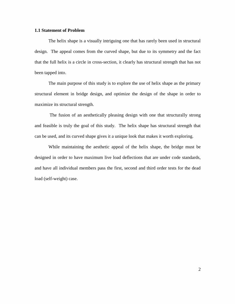
1.1 Statement of Problem
The helix shape is a visually intriguing one that has rarely been used in structural
design. The appeal comes from the curved shape, but due to its symmetry and the fact
that the full helix is a circle in cross-section, it clearly has structural strength that has not
been tapped into.
The main purpose of this study is to explore the use of helix shape as the primary
structural element in bridge design, and optimize the design of the shape in order to
maximize its structural strength.
The fusion of an aesthetically pleasing design with one that structurally strong
and feasible is truly the goal of this study. The helix shape has structural strength that
can be used, and its curved shape gives it a unique look that makes it worth exploring.
While maintaining the aesthetic appeal of the helix shape, the bridge must be
designed in order to have maximum live load deflections that are under code standards,
and have all individual members pass the first, second and third order tests for the dead
load (self-weight) case.

3
1.2 Designing Bridges for Aesthetics: Robert Maillart and Santiago Calatrava
Throughout history, structures have served a specific purpose. They are designed
and constructed with the purpose of making the lives of humans better in one way or
another. Whether it is for shelter, travel or financial profit, structures obviously play a
major part in the development of human civilization as it seen today.
The most notable structural device used for transportation purposes is the bridge.
Bridges have become recognizable landmarks across the world, sometimes becoming the
structure that defines a city or town. Although the purpose of a bridge is simply to carry
people and their goods across a gap, whether it be over water or a gap of another kind, it
is clear that bridges are much more than just transportation structures.
There are, of course, bridges with the simplest of designs; that do little more for
the eye than the roadway/railway surface they carry. Bridges of this nature our often
older, as they were built purely for practical purposes: getting people and goods from one
side to the other. It seems as if that simple design thought process has become a thing of
the past, and the design of a bridge is so much more than a simple structure that serves
physical needs.
Two men have been at the forefront of this change in thought. The first is Robert
Maillart, who spent much of his career innovating new ways in which one could make
designs normally considered outrageous technically feasible. Technical feasibility is the
obvious obstacle that must be overcome in order to make unique bridges, and this was
Rober Maillart’s life’s work: designing beautiful bridges that were once thought to be
technically infeasible. In doing this, he set a precedent for architects and structural
engineers alike. Bridges today are designed with a much higher emphasis on aesthetics

4
than they ever have been before, and it has become the norm, they are often considered
works of art. Works of art: with an extremely practical and important primary function.
Robert Maillart was born in Berne, Switzerland in February of 1872. As a
student, he was frustrated by the overemphasis often put on mathematics in structural
design, and rather “pioneered innovative research and design in direct opposition to
authorities and peer groups that had been seduced by the applied science view” [1].
Maillart believed that the emphasis on applied science in structural engineering
discouraged real innovation, and he thought that studying real life structures was a
significantly more effective way to come up with innovative bridge design. Maillart
studied the ways in which geometric shapes distributed forces, and he found “that elegant
appearance could arise from the patterns traced by these forces. Elegance arose from the
structure itself and not from an extraneous idea of beauty.” [1] It is this thought for which
Robert Maillart will truly be remembered.
In his attempts to create bridges not from classical applied science methods, but
from untraditional alternatives, he innovated many major design features that had never
before been seen in structural design. These included the concrete hollow box, the
concrete flat-slab floor, the concrete deck-stiffened arch, and the idea of shear center.
In the late 1800’s, iron was the main structural element being used in construction
projects. In his first opportunity to design a bridge in Switzerland, Maillart instead
designed a concrete single-arch bridge over the Sihl River in Zurich, known as the
Stauffacher Bridge.

5
Figure 1.2.1 – The Staffacher Bridge [1]
It was significantly more cost effective than the iron alternatives, and it used concrete
arch that did not contain reinforcement. The bridge was submitted against 3 other
designs, 2 of which were steel, the other concrete, and Maillart’s bridge was chosen as
the victor. The use of concrete was vitally important, as it was more aesthetically
pleasing than metal designs, and it was more lightweight and cost effective than
commonly-used stone designs. Maillart used 3 hinges, as shown in the figure on the
following page, one in the center of the arch and one on each end, and that allowed for
unreinforced concrete to be used without the stresses in the arch becoming unbearable.

6
Figure 1.2.2 – The Stauffacher Bridge’s three hinges [1]
It was at the turn of the century when the use of reinforced concrete had started to
become popular in design and construction. Maillart used reinforced concrete in his first
major innovation, the Zuoz Bridge. In this design, Maillart used an arch that was made
up of 2 hollow concrete boxes (connected by a vertical center wall), and his design was
unique in the fact that it allowed for the arch, walls and deck to carry the load, rather than
just the arch, as was done with more traditional designs.
Figure 1.2.3 – Cross-section of the Zuoz Bridge [1]

7
“Maillart stressed that the structure would have all of the virtues of stone but without its
great weight for, like steel, the concrete sections are reduced to a minimum” [1].
Figure 1.2.4 – A photograph of The Zuoz Bridge [2]
Maillart’s next major innovation was the use of the three-hinged arch, which he
popularized at the Rhine River Bridge at Tavanasa. The three-hinged arch was used in
other designs of his, but at Tavanasa, it was the main focus in this particular model. The
design allowed for the bridge to be extremely thin, which was both unprecedented and
visually appealing. “He created that innovation by expressing the three hinges as places
where the arch has minimum thickness, and between hinges, the arch fuses with the
horizontal deck to provide the necessary stiffening” [1]. Though completed in 1905, the
Maillart’s bridge over the Rhine River at Tavanasa has an extremely modern feel to it,
even by today’s standards.

8
Figure 1.2.5 – Cross-section of the bridge over the Rhine River at Tavanasa [1]
Figure 1.2.6 – Maillart’s drawings of the bridge over the Rhine River at Tavanasa [1]

9
Maillart’s technological breakthroughs in bridge design allowed him to fuse
together beauty with practicality and function. Without making any further major
engineering innovations, Maillart designed 3 bridges known primarily for their beauty in
the mid-1920’s. The first of these designs was the Valtscheilbach Bridge, which is best
known for having the thinnest arch of its time.
Figure 1.2.7 – A drawing of the Valtscheilbach Bridge [1]
“Its lyrical contrast of a light arch with a stout deck remains its primary delight” [1]. In
the past, Maillart’s designs had unique and relatively cheap to build, but they weren’t
necessarily known for their aesthetic appeal. The Valtshielback Bridge changed that
thought, as its thinness was not only financially practical, but undeniably beautiful.
Figure 1.2.8 – A photograph of the Valtscheilbach Bridge [1]

10
His next achievement in style came with the Chatelard, with which he insisted on
symmetry, despite what the landscape called for. Dealing with an asymmetrical ravine,
Maillart designed a symmetrical frame that would need a stone pedestal for one half of
the legs, while the other half set directly into the earth. “Maillart’s symmetrical frame
reflects his concern for a trouble-free structure more than for visual conformity to a given
landscape” [1].
Figure 1.2.9 – A drawing of the Chatelard [1]

11
Figure 1.2.10 – A photograph of the Chatelard [1]
The final bridge in the stretch was designed to carry the Swiss national railway
across the Grand Fey Viaduct. This massive undertaking was far larger than the other
bridges he had designed and constructed, and it posed a great technical challenge for
Maillart, as he was known for designing his concrete arched for unprecedented thinness.
“The arches and other vertical members are so light be comparison to the pillars that in
profile there is the same feeling of surprise as at Valtschielbach” [1]. Though massive,
Maillart was able to design a bridge that resonates with the eye just as his sleekest design
does, despite the fact that it has 6 arches to the Valtschielbach’s single arch, and covers a
much longer span.
12
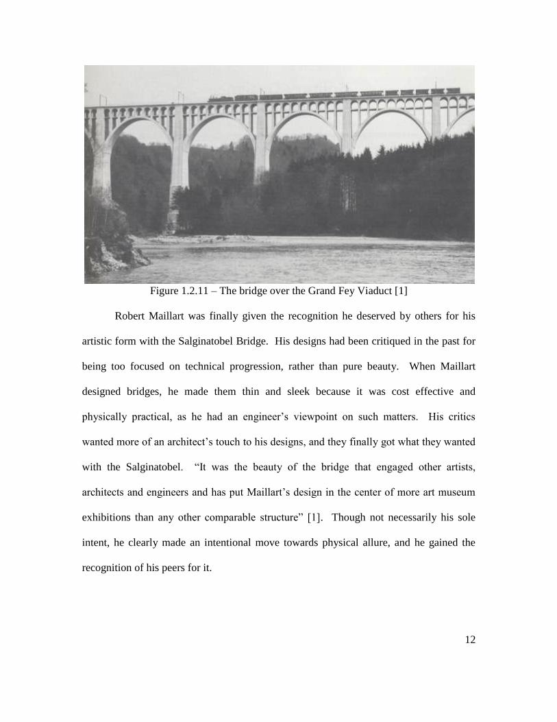
Figure 1.2.11 – The bridge over the Grand Fey Viaduct [1]
Robert Maillart was finally given the recognition he deserved by others for his
artistic form with the Salginatobel Bridge. His designs had been critiqued in the past for
being too focused on technical progression, rather than pure beauty. When Maillart
designed bridges, he made them thin and sleek because it was cost effective and
physically practical, as he had an engineer’s viewpoint on such matters. His critics
wanted more of an architect’s touch to his designs, and they finally got what they wanted
with the Salginatobel. “It was the beauty of the bridge that engaged other artists,
architects and engineers and has put Maillart’s design in the center of more art museum
exhibitions than any other comparable structure” [1]. Though not necessarily his sole
intent, he clearly made an intentional move towards physical allure, and he gained the
recognition of his peers for it.

13
Figure 1.2.12 – A photograph of the Salginatobel Bridge [3]
The second designer that has revolutionized the way bridge design is looked at in
the modern world is Santiago Calatrava. Born in Spain and educated in both architecture
and civil engineering, he has been able to fuse technical triumphs with breathtaking
visuals in bridge design like no other before him. His feats in the bridge design world go
virtually unmatched, and it is clear that his background as both an architect and a
structural engineer have had a huge impact on his designs.
“Calatrava has long maintained that bridges, as design objects, could combine
technological intelligence with poetry to enhance the sense of identity and cultural
significance of a particular place” [4]. Bridges throughout history have generally had one
singular focus: stability. Designers like Calatrava have made aesthetics equal in
importance to stability, without sacrificing anything from the latter. This achievement
has gone from a trivial pursuit for beauty, to a seemingly necessary part of the design
process, since the time Calatrava started designing bridges.

14
In his early career as a designer in the late 1970’s, Santiago Calatrava often drew
inspiration from real life forms in his bridge designs. He was influenced in his tubular
design for the Walensee Bridge in Switzerland by “the tubular limbs of birds, insects and
crustaceans” [4]. His next design, for the Acleta Alpine Motor Bridge in Disentis,
Switzerland, came about from, “In Calatrava’s own words, the ‘form of a bird’” [4]. He
went through multiple iterations in this particular design, constantly removing
unnecessary redundancies, and through them “the structure became even more
transparent, even more articulated, demonstrating more clearly the way forces traveled
through matter” [4]. It is clear through Calatrava’s early work that his form is beginning
to emerge, and it is a beautiful fusion of grace and stability.
Figure 1.2.13 – A model of the Walenesse Bridge [2]
15
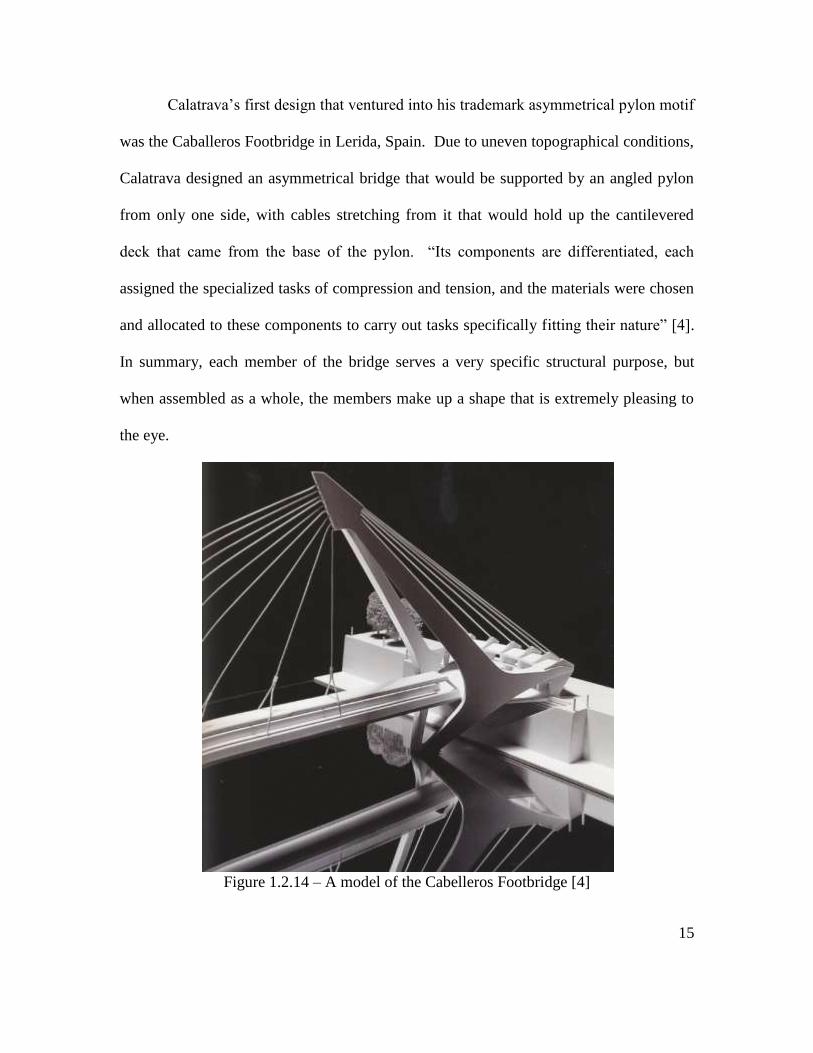
Calatrava’s first design that ventured into his trademark asymmetrical pylon motif
was the Caballeros Footbridge in Lerida, Spain. Due to uneven topographical conditions,
Calatrava designed an asymmetrical bridge that would be supported by an angled pylon
from only one side, with cables stretching from it that would hold up the cantilevered
deck that came from the base of the pylon. “Its components are differentiated, each
assigned the specialized tasks of compression and tension, and the materials were chosen
and allocated to these components to carry out tasks specifically fitting their nature” [4].
In summary, each member of the bridge serves a very specific structural purpose, but
when assembled as a whole, the members make up a shape that is extremely pleasing to
the eye.
Figure 1.2.14 – A model of the Cabelleros Footbridge [4]

16
Figure 1.2.15 – A model of the Cabelleros Footbridge (alternate view) [4]

17
Calatrava’s next two famous designs were constructed in Europe in the late
1980’s. The first was the Bach de Roda Bridge in Barcelona. Though designing a rigid
structure that is literally built to stay still, Calatrava’s main focus in this design was
movement. When referring to his design, Calatrava said “Mobility is implicit in the
concept of strength … strength is crystallized movement” [4]. This simply shows the
unique thought process that went into his bridges, and he also considered the actual
movement of people in vehicles in his design. Rather than make a pedestrian walkway
that would force people across in a thin straight line, Calatrava designed pedestrian
platforms on each side of the bridge (that jut out as half ovals from the sides) and stairs
leading up to them. This made this design more than just a bridge for transportation
purposes, which is clearly always on the forefront of his mind.
Figure 1.2.16 – A photograph of the Bach de Roda Bridge [5]

18
The second design of his constructed in the late ‘80’s was the Oudry-Mesly
Footbridge in Creteil-Paris, France. The arch spans above the bridge, clearly reminiscent
of a spinal column or back of an animal, giving it the previously mentioned life form that
Calatrava so often designed for.
Figure 1.2.17 – A photograph of the Oudry-Mesly Footbridge [6]
19
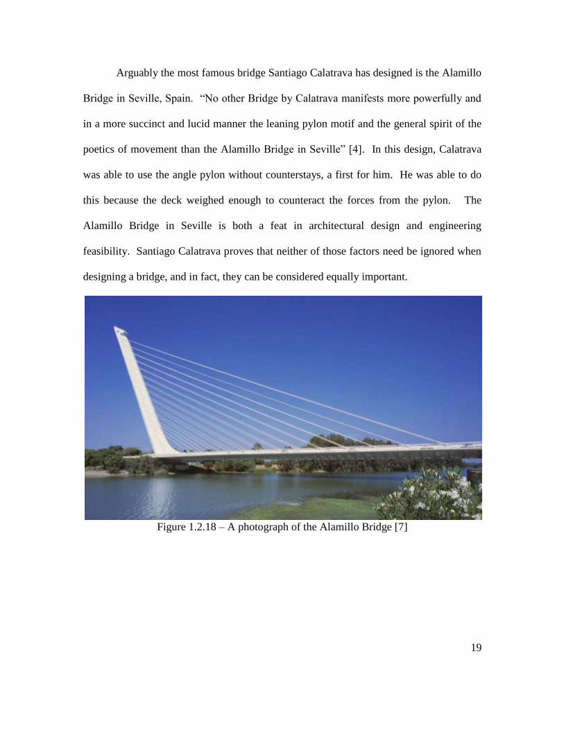
Arguably the most famous bridge Santiago Calatrava has designed is the Alamillo
Bridge in Seville, Spain. “No other Bridge by Calatrava manifests more powerfully and
in a more succinct and lucid manner the leaning pylon motif and the general spirit of the
poetics of movement than the Alamillo Bridge in Seville” [4]. In this design, Calatrava
was able to use the angle pylon without counterstays, a first for him. He was able to do
this because the deck weighed enough to counteract the forces from the pylon. The
Alamillo Bridge in Seville is both a feat in architectural design and engineering
feasibility. Santiago Calatrava proves that neither of those factors need be ignored when
designing a bridge, and in fact, they can be considered equally important.
Figure 1.2.18 – A photograph of the Alamillo Bridge [7]

20
Calatrava’s next aesthetic marvel was the Trinity Footbridge, which was
constructed in Salford, England in the mid-1990’s. Calatrava’s design needed to account
for the large differences in the heights of the riverbanks on either side of the bridge, and
that is why he chose to use the asymmetrical mast design, as the angle made up for the
change in elevation. This design is a perfect example of how the engineering criteria for
a project allowed for it to become visually pleasing, as the angled pylon stands out, while
the uneven river banks were the primary reason for necessity of the design.
Figure 1.2.19 – A photograph of the Trinity Footbridge [8]

21
Calatrava also took his beautiful pylon motif to the Netherlands, where he
designed 3 angled mast bridges in the town of Hoofddorp, known as The Lyre, The Lute
and The Harp. “As part of its infrastructure planning, the regional government resolved
to create bridges that would not only serve transportation needs but also function as
landmarks at main crossings over the Hoofdvaart to reflect the economic and social
changes affecting the region” [4]. The project was started in 1999, and it was clear that at
this point in time that the aesthetics of larger bridge projects had become equally
important to the engineering behind them. The tallest mast for this set of bridges is over
200 feet tall, which is almost twice as tall as the one for Calatrava’s Trinity Footbridge.
Figure 1.2.20 – A photograph of The Lyre [4]

22
One can now argue that the look and feel of a bridge has become more important
than its primary function as a structure for transportation. No longer can a bridge be
designed purely for function, it is a necessity to include the look of a bridge in every
phase of the design process. With advances in technology, the structural strength of a
bridge has become almost a given, and the aesthetic aspects of the bridge have become
the main focus of bridge design.

23
1.3 The Helix Bridge: Singapore
The first bridge in the world to use the helix shape as part of its structural design
was constructed in Singapore, and it is known simply as “The Helix” [9]. The 280 meter
long pedestrian bridge spans the Marina Bay, but requires multiple supports to cross the
gap, as can be seen in the figure below.
Figure 1.3.1 – The Helix Bridge in Singapore [9]
Although the main element supporting the bridge is the supports below, the helix is vital
to taking the load. The two repeating helical rings that make up the double helix
structure act together as a tubular truss, which allows the bridge to use 5 times less steel
than a conventional box girder bridge [9]. Although the helix shape is used as structural
element in the design of this bridge, it is clear that it is not the primary load bearing
element across the entire span, as the supports are needed. This is due to the fact that the
outer helical structure was not designed to distribute the loads across the entire span, only
to the supports, which are less than 100 meters apart. The helix shape is used primarily

24
as an architectural element with aesthetics as its primary function, but clearly has
structural strength.

25
1.4 Longest Steel Bridge Spans
The longest bridge spans in the world are cable-stayed or suspension bridge types,
as these designs are extremely strong while also having a significantly lower dead weight
than a steel girder bridge of similar length. The efficiency of the suspension bridge
allows for bridges to span distances of thousands of feet, with the longest in the world
being the Akashi Kaikyo Bridge in Japan, which spans a maximum distance of 6,532 feet
[10]. Due to the efficiency of these bridge types, they have become the primary choice
for long span bridges, and are the only bridge types that have spanned gaps of more than
1900 feet. The longest steel non-suspension or cable-stayed span bridges in the world are
the Chaotianmen and Lupu bridges in China, which are both steel arch bridges [11].
The Chaotianmen Bridge is located in Chongqing, China and was completed in
2009. With a span of 1,811 feet, it is the longest steel non-suspension or cable-stayed
bridge in the world. It uses two curved steel truss tied arches, which span the gap while
distributing the loads into the supports [12]. The deck is suspended from the arches, and
the bridge carries both vehicular traffic and rail traffic. The curved trusses also give the
bridge a look that is extremely appealing to the eye. When looking at the side view of the
bridge, one can clearly see how the bridge distributes the load from the center into the
supports at either end, as seen in the figure on the following page. It is also clear how a
steel span bridge must be designed, the maximum height above the supports is found at
the center, while the arches drive into the supports at the ends. This bridge only has
compression support on the top, as there is no need for tension support below the deck
because the bases of the supports are much lower than the deck that is being supported.

26
Figure 1.4.1 – The Chaotianmen Bridge [13]
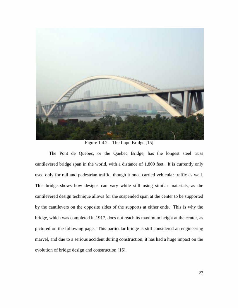
The next longest steel arch bridge is the Lupu Bridge in Shanghai, China, and it
spans a maximum distance of 1,804 feet. This bridge was completed in 2002, and was
the longest bridge of its kind upon its completion, until the aforementioned Chaotiamen
Bridge was completed in 2009. The arches meet at the center of the bridge at the highest
point, and drive directly into the ground at either end of the span. The steel arches, as
pictured on the following page, are over 29 feet thick and 15 feet wide in cross section,
which are unprecedentedly large when it comes to steel bridge design [14].
27
Figure 1.4.2 – The Lupu Bridge [15]
The Pont de Quebec, or the Quebec Bridge, has the longest steel truss
cantilevered bridge span in the world, with a distance of 1,800 feet. It is currently only
used only for rail and pedestrian traffic, though it once carried vehicular traffic as well.
This bridge shows how designs can vary while still using similar materials, as the
cantilevered design technique allows for the suspended span at the center to be supported
by the cantilevers on the opposite sides of the supports at either ends. This is why the
bridge, which was completed in 1917, does not reach its maximum height at the center, as
pictured on the following page. This particular bridge is still considered an engineering
marvel, and due to a serious accident during construction, it has had a huge impact on the
evolution of bridge design and construction [16].

28
Figure 1.4.3 – The Pont de Quebec [17]
Although the precedent for a steel bridge with a main span of more than 1800 feet
is apparent, designing one with a span of 2000 feet adds over 10 percent to the overall
length. The choice of the 2000 foot span length for the helix bridge in this study will
provide the challenge of designing the world’s longest steel bridge, while also using and
optimizing the helix shape.

29
2. Structural Background Information
A bridge is unique from other large structures due to the fact that it is made to
span distances without supports over a given distance. This makes the design of a bridge
significantly different from that of a building or other large structure. The following
sections cover the theory behind long span bridge design, the commonly used equations
in the field and information specific to the geometry of the helix shape.

30
2.1 The Simply Supported Beam
If a bridge is simplified to its most basic elements, it can be modeled as a beam
with pin supports at one end and roller supports at the other. This is also known as a
simply supported beam.
As is the case for a simply supported beam, the moment for a bridge span is
highest at the center, and this is the primary element that must be designed for when
designing a long span bridge. The moment and shear diagrams for a uniformly loaded
simply supported beam can be found in the figure on the following page, and they are
extremely similar to those experienced over a bridge span. The highest amount of shear
occurs at the ends of the bridge, at the supports, while the moment is equal to zero at
these same locations. The stress distribution in a simply supported beam is also very
similar to the way that forces are distributed at the center of the span of a bridge, and that
is shown on the lower figure on the following page. The top members above the road at
the center of the bridge span will be in the highest compression, while the members under
the roadway at the center of the bridge will experience the highest tension. The force,
moment and stress distribution in a simply supported beam shows why most long span
bridges look the way they do, the bridge members increase in height above the supports
(not necessarily the roadway) as they get closer to the center of the span.

31
Figure 2.1.1 – Moment and shear diagrams in a simply supported beam [18]
Figure 2.1.2 – Stress distribution in a beam [19]

32
2.2 Commonly Used Equations in Bridge Design
As shown in the previous section, a long span bridge can be modeled as a simply
supported beam. The equation for the moment in a uniformly loaded simply supported
beam is shown below [18]:
Where l is the length of the beam, w is the uniformly distributed load and x is the
distance from one end. This shape is also the optimum shape of an arch that can be used
in bridge design. If the arch follows the exact shape of the moment distribution curve, it
will provide the most efficient distribution of the force possible. This means that the
highest members above the supports at any point along the span of bridge that is perfectly
designed in this sense will follow the equation above, so that the bridge arch will make
the out the moment equation when viewed from the side of the span. For a bridge with
2000 foot span and a center height of 100 feet above the support, the equation for the
height above the support of the top-most member should be as follows for optimal
performance:
Where Z is the height in feet, x is the distance from the end support, 2000 is the span
length in feet and C is a coefficient that converts for the maximum height (h) desired at
the center of the bridge from the from the fact that the actual moment equation is based in
units for a uniformly distributed load, which includes units containing forces.

33
The next important equations to be discussed are for axial loads applied to
individual steel members in bridges. There are two main ways a member can fail,
reaching its yield strength and buckling. Buckling is more common and more worrisome
when dealing with the long members typically used in steel bridge design. The equation
for stress in a member is as follows:
Where P is the axial force and A is the cross-sectional area of the member [20]. If the
stress, σ, reaches the yield strength for the material, the member will begin to fail. The
yield strength for steel can vary, but the standard is 36ksi. It is more common for a steel
member to fail due to reaching its yield strength from a tensile axial force, because a
member under compression will typically buckle first. The buckling equation, known as
Euler’s equation, is shown below [20]:
Where Pcr is the critical force that causes buckling in a member with given values of
length (L), modulus of elasticity (E), radius of gyration (r) and moment of inertia (I).
This particular buckling equation is used for members connected by pins at both ends.
The equation for members with fixed ends uses the effective length of the members as
they are not as free to buckle, which is found to be approximately L/2.
The next equations important to bridge design are those for the maximum
allowable live load deflections. A bridge must be designed so that it can handle the live
load without deflecting considerably, according to code standards. If the bridge deflects

34
too much, it will be noticeable to the traffic crossing the bridge, which is not allowable.
The equations for the maximum allowable live load deflections are found below [21].
For standard bridges:
For bridges with pedestrian traffic:
Where L is the length of the bridge and ΔLL is the maximum allowable live load
deflection. The maximum allowable live load deflection is based purely on the length of
the bridge, and a 2000 foot span has a maximum allowable live load deflection of 2.5 feet
(30 inches) for standard bridges, and a maximum allowable live load deflection of 2 feet
(24 inches) for a bridge with pedestrian traffic.

35
2.3 The Helix Shape
A helix is essentially a spiral shape, which is a circle dragged out in a third
dimension. The “double-helix” shape is best known for being the shape of DNA, which
was discovered by James Watson and Francis Crick in 1953 [22]. In theory, the helix is a
smooth shape, but for design purposes, the helix must be divided into straight line
segments. These straight line segments still give the look and structural integrity of the
helix, while also making construction technically feasible. Parametric equations are used
in order to determine the points for which a helix intersects. These parametric equations
are shown below [22]:
The t value that is used is the angle (in radians), about the origin. The x and z
coordinates make the shape of a circle with constant radius a. The y coordinate is
determined using the pitch, or length, of the helix, where the pitch is defined as 2πb,
where b is the length. The y-coordinate increases as the x and z coordinates circle around
the y-axis, giving the desired helix shape. For construction purposes, the helix must be
divided into segments. Therefore, for a “half-helix”, the total angle of rotation is π across
the span of a bridge, while a “full-helix” has an angle of rotation of 2π across the span of
the bridge.
36
3. Autodesk Robot Structural Analysis
The structural analysis program used in the analyses for the design and
optimization of the helix bridge is Autodesk Robot Structural Analysis Professional 2012
(Robot). The following section is a step-by-step guide on how to construct a helix shaped
bridge in Robot, and how to go about analyzing it for live and dead load (self-weight)
cases for first, second and third order tests. The most helpful tool for learning to use
Autodesk Robot is the User’s Guide [23], and any user is encouraged to supplement the
guide in this section with the User’s Guide provided by Autodesk. All of the figures
found in the following sections are taken directly from the program.

37
3.1 Modeling a Helix Shaped Bridge in Robot
The focus of this section will be to guide a user through the process of
constructing a helix shape bridge in Autodesk Robot Structural Analysis Professional
2012. The user will learn to model the helix shape based on a set on pre-defined
parameters, and analyze the dead and live load deflections using Robot.
The first step is to define the parameters that the bridge must be designed for. In
this example, a 2000 ft span will be used. The first step is to choose the radius of the
helix. In a view of the bridge from one of its ends down its full length, the helix makes a
perfect circle. The radius of this circle needs to be chosen by the designer in order to
construct the model. This radius can be optimized, but a starting radius must be chosen
in order to start the process.
The helix shape is, in reality, a perfect circle extended in a third dimension. For
the purposes of construction feasibility, the helix must be broken into segments, as it
cannot be constructed as a perfect helix for the length of the span. For this example, the
segments will be 40 feet along the deck of the bridge (40 feet in the y-direction). For the
2000 foot span, this division will create 50 sections. The length of each member of the
helix will be slightly longer than 40 feet, due to the fact that it is connecting the 40 feet in
the y-direction over an angle. After defining this step, the points of the helix can then be
found.
Using Microsoft Excel, the helix equation can be input in order to find the node
locations where each member of the helix will connect. The equations are as follows:
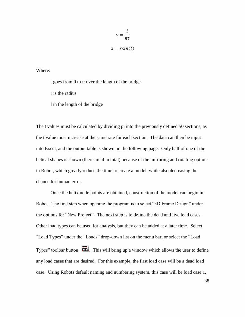
38
Where:
t goes from 0 to π over the length of the bridge
r is the radius
l in the length of the bridge
The t values must be calculated by dividing pi into the previously defined 50 sections, as
the t value must increase at the same rate for each section. The data can then be input
into Excel, and the output table is shown on the following page. Only half of one of the
helical shapes is shown (there are 4 in total) because of the mirroring and rotating options
in Robot, which greatly reduce the time to create a model, while also decreasing the
chance for human error.
Once the helix node points are obtained, construction of the model can begin in
Robot. The first step when opening the program is to select “3D Frame Design” under
the options for “New Project”. The next step is to define the dead and live load cases.
Other load types can be used for analysis, but they can be added at a later time. Select
“Load Types” under the “Loads” drop-down list on the menu bar, or select the “Load
Types” toolbar button: . This will bring up a window which allows the user to define
any load cases that are desired. For this example, the first load case will be a dead load
case. Using Robots default naming and numbering system, this case will be load case 1,

39
Table 3.1.1 – Helix Bridge: Node Points
Radius =100ft Length=2000ft
T x Y z
0 100.00 0 0.00
π/50 99.80 40 6.28
2π/50 99.21 80 12.53
3π/50 98.23 120 18.74
4π/50 96.86 160 24.87
5π/50 95.11 200 30.90
6π/50 92.98 240 36.81
7π/50 90.48 280 42.58
8π/50 87.63 320 48.18
9π/50 84.43 360 53.58
10π/50 80.90 400 58.78
11π/50 77.05 440 63.74
12π/50 72.90 480 68.45
13π/50 68.45 520 72.90
14π/50 63.74 560 77.05
15π/50 58.78 600 80.90
16π/50 53.58 640 84.43
17π/50 48.18 680 87.63
18π/50 42.58 720 90.48
19π/50 36.81 760 92.98
20π/50 30.90 800 95.11
21π/50 24.87 840 96.86
22π/50 18.74 880 98.23
23π/50 12.53 920 99.21
24π/50 6.28 960 99.80
25π/50 0.00 1000 100.00

40
and it will be labeled as “DL1”. To add the case, select “dead” under the “Nature” drop-
down menu, and then click “Add”, and DL1 will be added to the list of defined cases
below. The next load case that needs to be added will be the live load case, and it will be
defaulted as case number 2 and labeled “LL1”. To add it, select “live” under the
“Nature” drop-down list and click “Add”. The “Load Types” window will look like the
figure below once the cases have been defined:
Figure 3.1.1 – The “Load Types” window
41
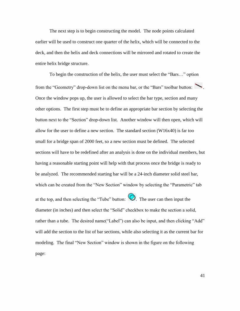
The next step is to begin constructing the model. The node points calculated
earlier will be used to construct one quarter of the helix, which will be connected to the
deck, and then the helix and deck connections will be mirrored and rotated to create the
entire helix bridge structure.
To begin the construction of the helix, the user must select the “Bars…” option
from the “Geometry” drop-down list on the menu bar, or the “Bars” toolbar button: .
Once the window pops up, the user is allowed to select the bar type, section and many
other options. The first step must be to define an appropriate bar section by selecting the
button next to the “Section” drop-down list. Another window will then open, which will
allow for the user to define a new section. The standard section (W16x40) is far too
small for a bridge span of 2000 feet, so a new section must be defined. The selected
sections will have to be redefined after an analysis is done on the individual members, but
having a reasonable starting point will help with that process once the bridge is ready to
be analyzed. The recommended starting bar will be a 24-inch diameter solid steel bar,
which can be created from the “New Section” window by selecting the “Parametric” tab
at the top, and then selecting the “Tube” button: . The user can then input the
diameter (in inches) and then select the “Solid” checkbox to make the section a solid,
rather than a tube. The desired name(“Label”) can also be input, and then clicking “Add”
will add the section to the list of bar sections, while also selecting it as the current bar for
modeling. The final “New Section” window is shown in the figure on the following
page:
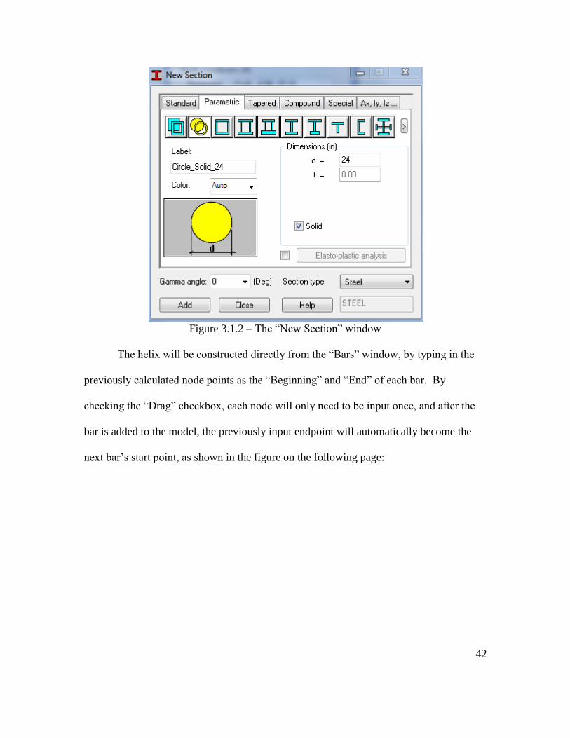
42
Figure 3.1.2 – The “New Section” window
The helix will be constructed directly from the “Bars” window, by typing in the
previously calculated node points as the “Beginning” and “End” of each bar. By
checking the “Drag” checkbox, each node will only need to be input once, and after the
bar is added to the model, the previously input endpoint will automatically become the
next bar’s start point, as shown in the figure on the following page:

43
Figure 3.1.3 – The “Bars” windows. The first bar created in the helix is shown on the
left, while the second is on the right.
Once the first half is complete (y=1000ft), the bridge should look as it does below from
the “Front” view on the 3D view cube (The cross section looking down the bridge should
be a perfect quarter-circle):
Figure 3.1.4 – Helix quarter-circle cross-section
44
To view the bridge in this way, the” Dynamic View” option must be selected
from the “View” drop-down list on Menu Bar, which will make the model viewable in
3D space. The next step is to create the deck. The deck will be created before the rest of
the helix members are copied, as the connections can be copied as well.
In this example, the deck will be a simple, flat deck with 40-foot sections. The
same procedure can be used to create a deck of any thickness, and a thicker deck will
give better results, but for the purposes of this model, the flat deck will be created. To
start, a bar must be drawn and then copied for the length of the bridge. The user can
select the “Bars” button and then type in the start and end points of the first bar of the
deck. In this example, the deck will be 50 feet wide, with four 10-foot lanes, and space
for pedestrian walkways. To create this, a bar must be created with a beginning point of
(-25,0,0) and an end point of (25,0,0). The user must then select the bar, and then select
the “Move/Copy…” option from the “Edit” pull-out list, which is found under the
“Edit” drop-down list on the menu bar. The “Translation” window will open, and the
input for the copy should be (0,40,0) in the “Translation vector” box, and the “Number of
repetitions” should be input as 25 (window shown below), which will create half of the
bridge deck sections.

45
Figure 3.1.5 – The “Translation” window
The deck sections will be created once the translation is executed. If the deck has
multiple levels or a thickness, the user can create the deck by selecting all of the members
that need to be copied. Only the first section needs to be drawn. After the deck sections
are visible, the deck members should be connected. This can be done by selecting the
“Bars” button, and then physically selecting the start and end points of the bar to be
inserted, rather than typing in the start and end points in the window. A single bar can be
input to connect the end of the first section to the end of the last on each side of the deck.
The 1000-foot long member that is created can then be divided into 40-foot sections be
selecting the “Intersect” button from the “Edit” drop-down list, which will
automatically create bar endpoints at every intersection for the entire structure. The
endpoint of each deck section should then be connected to the corresponding endpoint of
each helix section, so that each deck section connects to a helix section, and the y-value
46
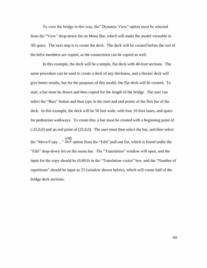
of the connection bar should remain constant. Once all of the connections are input, the
cross-section and side view of the bride should look as pictured below:
Figure 3.1.6 – Cross-section of the quarter helix with deck connections
Figure 3.1.7 - Cross-section of the quarter helix with deck connections
The next step is to mirror the helix and connection bars (not the deck), in 2 planes.
First, the user must select all of the non-deck members, and then mirror them over the
horizontal plane. Once the members are selected, the “Horizontal Mirror…” option
must be selected from the “Edit” pull-out list on the “Edit” drop-down list on the menu
bar. The user must then select any point on the x-y plane, and the bars will be mirrored
over the plane. The next step is to again select all of the non-deck members, and then use
the “Vertical Mirror…” option, which is found next to the “Horizontal Mirror”
option. The user must select a point on the y-z plane, and the members will be mirrored
across it. The result of each mirroring is shown in the figures on the following page:

47
Figure 3.1.8 – Cross-sections after the horizontal (left) and vertical (right) mirrors
Figure 3.1.9 – Isometric view of half of the helix bridge

48
The half bridge will then be rotated about itself, and the entire bride will be created. This
is done by selecting all of the members, and then using the “Rotate…” option,
which is found next to the horizontal and vertical mirror options. The user must then
change the “Axis end” to the X-Y plane by selecting the “Plane” circle. Then, the point
that the bridge will be rotated about must be selected (select any point where x = 0 and y
= 1000). The “Angle” must be input as 180 degrees, and the full bridge will be created
when the “Execute” button is clicked. The final inputs are shown in the figure below:
Figure 3.1.10 – The “Rotation” window
The full bridge should be visible after the rotation step is complete. The next steps are to
add the end supports and the live load, which will complete the basic model.

49
The bridge end supports should be pinned on one end with rollers on the other. The
pinned end support is a standard Robot support (along with fixed), but the roller end
support must be created. To do this, the user must select the “Supports…” option from
the “Geometry” drop-down list on the menu bar, or the “Supports” button on the
toolbar. The window that opens will have an option to create a new support, and
selecting this will open the “Support Definition” window. For the roller support, the
“Fixed directions” that should be checked are UX and UZ (under the “Rigid” tab). UY
should not be selected so that the end is free to roll in that direction. The pinned and
roller supports can then be added to the ends of the bridge by selecting the appropriate
support, and then selecting the node on the model where the support is wanted. 8 total
supports should be put on the model, four pinned supports at the four nodes at y = 0’, and
four roller supports at the four nodes where y = 2000’.
In order to load the bridge with a live load from the traffic, an area must be
created that the load will be distributed over. A cladding must be created, and it will act
as the roadway for the purposes of distributing the load. The user must select the
“Claddings…” option from the Geometry drop-down list, and a window will open
prompting the user to enter the cladding definition. The load distribution should be
selected as “Two-way”, and the definition method should be “Rectangle”. Selecting the
“Geometry” button will open an option to input three points, and the three points input
should create a cladding that is 40 feet wide (four 10-foot lanes), 2000 feet long and is
centered on the deck. The user must then load the created cladding with the live load.

50
The “Load Definition” button should be selected (from the “Loads” drop-
down list) in order to load the cladding. The model must be in load case 2, LL1, in order
to input the live loading. The “Uniform Planar Load” should be selected from the
“Surface” tab, as this will distribute the load throughout the cladding evenly, which is the
desired result. The input load should be 64psf (standard live load for bridges) in the
negative Z-direction. The input must be -0.064 kips/ft2 in the “Z” box, and by clicking
“Add”, the user can select the cladding, and the load will be distributed on it. The load
can be viewed on the cladding if the “Load symbols” option is on (this option is on a bar
at the bottom of the model space, next to the right-left scroll bar), and the red arrows will
be visible.
Figure 3.1.11 – Isometric view showing the pinned end supports, cladding and live load.

51
To analyze the model, the user must select the “Calculations” option in the
“Analysis” drop-down list on the menu bar. The program will then analyze the bridge,
and the results will become available. A full guide on how to analyze this model is
shown in the following section. For this particular model, the deflections will be too high
for the bridge to pass inspection. The model must optimized through an analysis of the
shape, and the various member sections must also be optimized to ensure strength while
minimizing the dead weight. This process for this analysis is shown throughout the
coming sections of this paper, and it can be used a guideline for optimizing the bridge for
a given set of parameters.
Figure 3.1.12 Isometric view showing the completed model.
52
3.2 Analyzing a Helix Shaped Bridge in Robot
After completing a model in robot, the next step in the process is to analyze it.
When the model is analyzed, the problems and flaws can be found, which are needed in
order to optimize the design of the bridge. In this section, the bridge will be analyzed for
live and dead load cases for both first and second (non-linear) order analyses using
Autodesk Robot Structural Analysis Professional 2012. This section is only a guide on
how to perform the analysis using Robot, the actual optimization of the helix bridge
begins in the next section.
Using the bridge model created in the previous section, the first step is to run a
basic first order analysis for both the dead and live load cases. To analyze the model, the
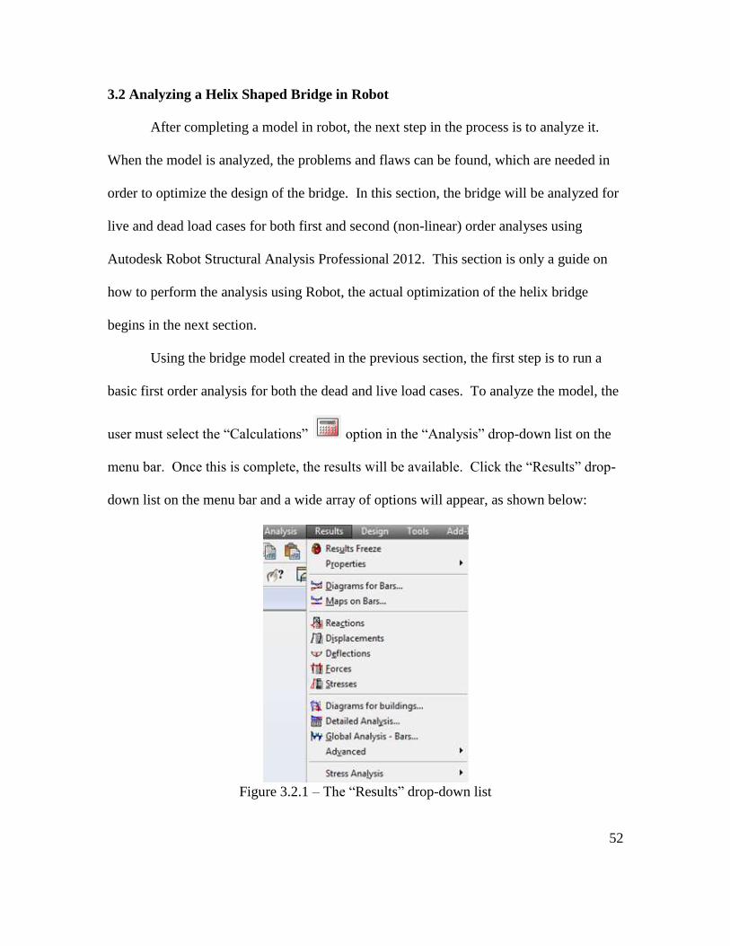
user must select the “Calculations” option in the “Analysis” drop-down list on the
menu bar. Once this is complete, the results will be available. Click the “Results” drop-
down list on the menu bar and a wide array of options will appear, as shown below:
Figure 3.2.1 – The “Results” drop-down list

53
The options on this menu are numerous and are all important to the overall design of a
bridge, but the main focus in this experiment is the maximum deflections of the bridge.
The deflections referred to in the results list are actually for individual bars, which are not
desired for this section. The desired values for this study are referred to in Robot as
displacements, which is how much each node displaces from its original starting point.
The maximum any node displaces on the bridge is the maximum deflection of the bridge.
Please note that whenever there is trouble with viewing options, select the “View”
drop-down list on the main menu bar, and then select “Structure View” (which is only
available if not already in Structure View), next select “Zoom” and “Zoom All”, and the
model should reappear at the center of the window.
To quickly find the maximum displacement of the bridge, the “Displacements
(deformation)” button should be selected. It is found in the lower right corner of the
model screen. Selecting this option will show the deflected shape of the bridge and give
the maximum deflection for each load case. To select the live load case, click the
“Cases” drop-down arrow (on the toolbar with the “Nodes” and “Bars” drop-downs) and
select “2: LL1”. The deformed shape should look like the figure below:
Figure 3.2.2 – Side-view of the live load deflected shape
If all of the steps followed in the previous section were followed exactly, the
maximum displacement should be approximately 61.4 inches. This is far too high, as the
maximum allowable displacement (or overall bridge deflection) is 30 inches, but the
techniques used to lower the maximum bridge deflections are shown in the following

54
sections. The maximum first order dead load deflection can also be viewed by selecting
the dead load case (1: DL1), from the “Cases” drop-down arrow (on the toolbar with the
“Nodes” and “Bars” drop-downs). The deformed shape will appear if the
“Displacements (deformation)” button is selected, and the maximum dead load
displacement should read approximately 455.0 inches (an extremely high value that will
be reduced in the following sections).
The next type of analysis is for second and third order types. There are two ways
to access the analysis types window, the first of which is to click the “Analysis
Parameters” button on the main toolbar (next to the calculations button). The other
way is to click the “Analysis” drop-down list on the main menu bar, and select “Analysis
Types”. The Analysis Types window will appear, as shown in the figure below:
Figure 3.2.3 – The “Analysis Type” window

55
In order to change the analysis type, select the desired load case and click the
“Parameters” button, which will bring up the “Nonlinear Analysis Parameters” window,
as shown below:
Figure 3.2.4 – The “Nonlinear Analysis Parameters” window
To select a second order analysis, check off the “Non-linear analysis” box, then click
“OK”, and the analysis type for the load case will change (note that if the model has
current analysis results, a warning will appear any time a change is made to it, just click
“Yes” to continue). If a third order analysis is desired, check off the “P-delta analysis”
box (which will auto select the non-linear case as well). If done correctly, the “Analysis
Type” should change to read “Static - Nonlin” for a second order analysis or “Static -

56
Nonlin.PD.” for a third order analysis.
Once the analysis type is change to second (or third) order, the calculations should
be run again. A different analysis window will appear, and the analysis will be run. This
is a more time consuming calculation as it requires multiple iterations, and there are two
common errors that will be viewed if there is failure, both of which are pictured below:
Figure 3.2.5 – Non-linear analysis failure notifications
If either of these two dialogue boxes appears, the bridge model has failed the second
order analysis. The first dialogue box means that the members in the model are bending
and displacing so much the non-linear analysis is not converging, meaning the shape is
deforming so badly that the bridge cannot pass the second order tests. The second
dialogue box implies that a member or, most likely, multiple members are buckling due
to the axial forces applied to them. Either of these notifications implies failure of the

57
analysis, and that the bridge model must be strengthened.
The next step is to analyze which members are failing. When the failure is due to
a non-convergence of the nonlinear problem, the program does not allow for the user to
view which members are the failing ones. The best way to figure out which members are
performing the worst is to go back to the linear first order analysis type, as the members
are still experiencing the same proportion of forces to the other members as in the higher
order analyses. Using the live load case under a first order analysis, running the
calculations again will produce the same results as found earlier. To analyze the
individual members, select the “Design” drop-down list on the main menu bar, and then
select “Steel Members Design – Options”, followed by “Calculations”, and the following
window will appear:
Figure 3.2.6 – The steel member design “Calculations” window
The next step is to make a couple of changes to the settings. First, make sure ever
member is actually selected to be analyzed by clicking the top “List” button and then
selecting “All” at the top. Next, change the load cases to just Case 2 (the live load case)

58
by selecting it after clicking the “List” button in the “Loads/Cases” area of the window.
Also uncheck the “Save calculation results” and the “Serviceability” boxes, as these are
not needed, but each has a corresponding warning/dialogue box. Note: If the design
parameters call for non-custom sections (meaning standard I-beams like W4x16 will
suffice), the optimization options can be used, and the program will automatically select
the optimal beams, but that is not possible for a bridge with all custom members. The
final window with the appropriate setting should look as below:
Figure 3.2.7 – The final steel member design “Calculations” window
Next, click “Calculations” at the bottom, and another window will appear. These are
the calculation results for each individual members based on the standards in ANSI/AISC
360-05 (the code parameters can also be changed). The code calculations produce an
efficiency ratio, which needs to be less than 1.00 to pass the tests. If the ratio is greater
than 1, the member is failing. The higher the efficiency ratio, the greater the need to
strengthen that member, as any member that has an efficiency ratio near or above one
will fail the second order tests. In this case, the live load members all pass, with some

59
members coming back with instabilities, which is normally due to excessive length.
Running the calculations again with the dead load case shows that most of the members
are failing; and therefore, they must be strengthened. The figure below shows some
passing (green) and failing (red) members due to the first order dead load analysis:
Figure 3.2.8 – Steel member calculation results for the first order dead load case
The techniques on how to reduce the failures and pass the appropriate tests are
shown in the following sections. The ability to model and analyze the bridge models in
Autodesk Robot Structural Analysis Professional 2012 is vital to proceeding with the
optimization of the helix bridge design.

60
4.0 Optimizing the Helix Bridge Structure for Live Load Deflections
A starting point for the optimization of the helix shape is chosen to be a 65 foot
radius in cross-section with a flat 65 foot wide deck. The span length of 2000 feet is
divided into 50 sections (40 feet each), with pin supports on one end of the bridge and
rollers on the other. The members are chosen to be 22.5 inch thick solid steel circles with
a yield strength of 36ksi. The helix is connected to the 65 foot wide bridge deck by
connecting one member directly from the helix to the edge of the deck at the intersection
of every 40 foot section. The live load is modeled as a 60 foot wide slab with a live load
force of 65 psf, while the dead load is from the self-weight of the bridge members. Some
images of the initial bridge model can be found on the following pages.
After performing an analysis in Robot using these established initial parameters, it
becomes clear that the bridge must be strengthened. The maximum live load deflection
of this bridge model is 95.7 inches, which is well over the allowable 30 inches for a 2000
foot span. The dead load deflections are even greater, having a maximum of 473.2
inches. The exaggerated deflected shape can also be seen on the following pages.
Using the results from the initial model, the optimization process can begin. The
main problem with this design is shear at the ends of the bridge, as can be clearly seen in
the deflected shape. Although the maximum deflection point of the bridge model occurs
at the center as expected, it is clear that the weakness in the model is at the ends. As can
be seen in the image, the majority of the bridge deflection occurs in the sections near the
ends of the bridge, whereas the middle sections do not deflect significantly compared to
the rest. In fact, the deflection in the first four forty-foot sections from the live load is
70.9 inches, while the next 21 sections only deflect an additional 24.8 inches to the

61
maximum at the center of the bridge.
The center of the bridge is strong due to the fact that the helix reaches its highest
point at the center, which is certainly where the most strength is needed, but this strength
is not distributed efficiently enough to the supports at the ends of the bridge. The flaw in
this early design is the thinness of the bridge at its ends near the connections, which are
clearly not strong enough to resist the load.
Using the initial results from the 65 foot radius model, the optimization of the
helix shaped bridge can begin. There are many variables that can be changed in order to
try and strengthen the bridge, which include: increasing the radius of the cross-section of
the bridge (or, more importantly, increasing just the height in the Z-plane), increasing the
thickness of the deck, adding a slope to the deck, changing the member sections,
increasing the yield strength of the steel, changing the shape of the outer support structure
and adding bracing or supports where needed.
Figure 4.0.1 – Cross section in the X-Z plane with a 65 foot radius.

62
Figure 4.0.2 – Isometric view.
Figure 4.0.3 – Side view in the Y-Z plane with a 2000 foot length
Figure 4.0.4 – Side view of the exaggerated deflected shape in the Y-Z plane. The
deflection in the end sections is seen to be greater than in the center sections.
63
4.1 Radius Size Optimization
The first parameter to be optimized will be the radius (or height) of the bridge, as
this is the most important factor when addressing the overall strength of the bridge. The
bridge can be braced at the ends and the member sections can be strengthened, but if the
height of the bridge at the center is not tall enough, there is no way the models will be
able to pass any of the relevant tests and standards, as they will not be strong enough.
To start this process, multiple models are produced with varying radii, and even
varying height to width ratios. The first step is to figure out what seem to be the optimal
height and width of the bridge cross section. Because of the number of parameters that
will change throughout the optimization process, the results from this particular analysis
will have to be re-optimized once the other parameters are finalized. This simply means
that adding a deck or increasing the area of the member sections might change the
optimal radius/height, as the weight of the bridge and the way forces are distributed will
change as various parameters are altered throughout the analysis.
To start this portion of the analysis, multiple bridge models will be analyzed using
various radii and height to width ratios. For the purposes of aesthetics, the ideal scenario
will be a helix shape bridge which forms a perfect circle in cross-section, meaning a
bridge with equal height and width. Increasing the height to width ratio will cause the
bridge to look like an oval in cross-section. All of the models in this section will cover
the 2000 foot span using a 65 foot wide flat deck that connects to the helix structure
every 40 feet. The members are all 22.5 inch solid steel circles (in cross-section), with a
yield strength of 36 ksi.
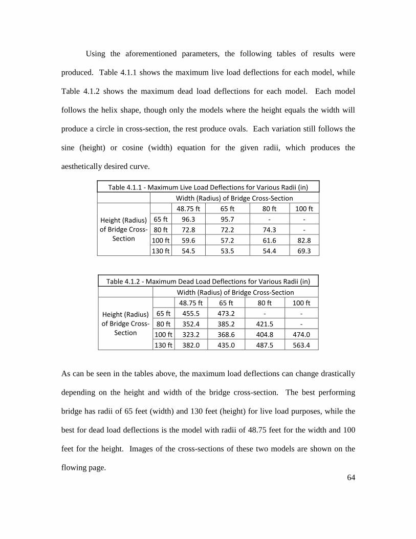
64
Using the aforementioned parameters, the following tables of results were
produced. Table 4.1.1 shows the maximum live load deflections for each model, while
Table 4.1.2 shows the maximum dead load deflections for each model. Each model
follows the helix shape, though only the models where the height equals the width will
produce a circle in cross-section, the rest produce ovals. Each variation still follows the
sine (height) or cosine (width) equation for the given radii, which produces the
aesthetically desired curve.
Table 4.1.1 - Maximum Live Load Deflections for Various Radii (in)
Width (Radius) of Bridge Cross-Section
Height (Radius) of Bridge Cross-
Section
48.75 ft 65 ft 80 ft 100 ft
65 ft 96.3 95.7 - -
80 ft 72.8 72.2 74.3 -
100 ft 59.6 57.2 61.6 82.8
130 ft 54.5 53.5 54.4 69.3
Table 4.1.2 - Maximum Dead Load Deflections for Various Radii (in)
Width (Radius) of Bridge Cross-Section
Height (Radius) of Bridge Cross-
Section
48.75 ft 65 ft 80 ft 100 ft
65 ft 455.5 473.2 - -
80 ft 352.4 385.2 421.5 -
100 ft 323.2 368.6 404.8 474.0
130 ft 382.0 435.0 487.5 563.4
As can be seen in the tables above, the maximum load deflections can change drastically
depending on the height and width of the bridge cross-section. The best performing
bridge has radii of 65 feet (width) and 130 feet (height) for live load purposes, while the
best for dead load deflections is the model with radii of 48.75 feet for the width and 100
feet for the height. Images of the cross-sections of these two models are shown on the
flowing page.

65
Figure 4.1.1 – Cross-sections of the best performing radius optimization designs.
The 65 foot (radius) width by 130 foot (radius) height model is shown on the left, while
the 48.75 foot (radius) width by 100 foot (radius) height is shown on the right.
An analysis into the data given produced makes it clear that increasing any
parameter will not always add strength to the bridge model. For the dead load cases, this
is clearly due to the fact that once the bridge is too large, it has more trouble supporting
itself, which causes greater deflections. Because the first priority in the analysis is to get
the maximum live load deflections within the allowable standards, the next step is to try
and optimize the model that performed best for live load deflections. For each height in
the live load analyses, the best performing model was always the one with a 65 foot
radius width. The next step is then to take this assumed optimal width, and optimize the
height that will produce the overall lowest live load deflections. This will be done by
producing multiple models with a 65 foot radius width at varying heights, and again
seeing which model has the lowest maximum live load deflections.

66
Keeping all other parameters the same, the models are analyzed again using
Robot, and the table shown below is a summary of the results, while the figure shown the
graph of the data. The models were also tested for dead load maximum deflections, as
this will become a more important parameter later in the optimization process.
Table 4.1.3 - Maximum Deflections for 65 foot Radius (Width) Models of Varying Height
Height: 65 ft 80 ft 105 ft 130 ft 150 ft 172.5 ft 215 ft 315 ft
Max. Live Load Deflection (in)
95.7 72.2 59.2 53.5 56.6 62.9 76.9 104.2
Max. Dead Load Deflection (in)
473.2 385.2 372.8 435.0 522.2 644.1 924.6 1635.2
0.0
20.0
40.0
60.0
80.0
100.0
120.0
0 50 100 150 200 250 300 350
Max
imu
m L
ive
Lo
ad D
efe
lcti
on
s (i
n)
Bridge Height (ft)
Figure 4.1.2 - Maximum live load deflections for 65 foot width models of varying height

67
The graph of the data in the figures makes it very clear as to what the desired radial
height of the bridge should be, though there is a large difference between the optimal
height to resist live load versus the optimal height to resist the bridge’s self-weight. The
optimal height for live load deflections is clearly very close to 130 feet (for this particular
set of variables), while the optimal height to resist the dead load seems to be very close to
100 feet, which is a fairly large difference. This is due to the fact that as the bridge gets
taller, it also gets heavier, and the increase in the self weight of the model outweighs the
increase in the strength of the model given by the larger height, and this turning point is
right around a 100 foot radius.
The maximum displacement values are important for comparison and also for
passing the relevant allowable standards, but looking at the manner in which the bridge is
0.0
200.0
400.0
600.0
800.0
1000.0
1200.0
1400.0
1600.0
1800.0
0 50 100 150 200 250 300 350
Max
imu
m D
ead
Lo
ad D
efe
lcti
on
s (i
n)
Bridge Height (ft)
Figure 4.1.3 - Maximum dead load deflections for 65 foot width models of varying height

68
deflecting can help the analysis progress drastically. This will be done by taking the 65
foot by 130 foot radius model and looking at its deflected shape, which is shown in the
figures below and on the following page.
Figure 4.1.4 – The exaggerated deflected dead load shape of the cross-section of the 65
by 130 foot radius model.

69
Figure 4.1.5 – The exaggerated deflected dead load shape of the side-view of the 65 by
130 foot radius model.
Figure 4.1.6 – The exaggerated deflected dead load shape of the isometric view of the 65
by 130 foot radius model.
The deflected shapes shown in the previous images are extremely exaggerated, but this
exaggeration helps make the flaws in this early design easily visible. The main two

70
problems are glaring in these figures, and they are the shear due to the thinness of the
bridge at the ends (as discussed in the previous section) and the lack of support of the
helix structure from about the quarter point of the bridge to the end. The outer helical
structure is not well supported towards the ends of the bridge, unlike at the middle. The
members that connect the helix to the deck towards the center of the bridge are near
vertical (in the x-z plane), whereas towards the ends, they approach being completely
horizontal. Because the self-weight from the helix is clearly all applied in the negative
vertical direction due to gravity, the more horizontal the members are, the weaker they
are in resisting the dead load. This causes the upper half of the helix to bow-out, as seen
in the figures, where as the bottom half of the helix simply sinks in towards itself (in the
exaggerated deflection, the bottom half of the helix actually overlaps in the image, but
this is only due to the excessive exaggeration).

71
4.2 Deck Thickness Optimization
In order to address the excessive deflections found in the flat deck bridge models
in the previous section, the next step in the optimization will be to add a thicker deck, and
see the effect it has on the deflections. Just as Robert Maillart first proved with the Zuoz
Bridge, the deck can be used as part of the structure to increase the overall strength in
resisting loads.
In this section of the analysis, a deck thickness will be added in order to help the
bridge resist the shear it is experiencing at its ends. Rather than adding a thick 65 foot
wide deck, the models with the deck will have a double deck that is 40 feet wide, which
will allow for three 10-foot lanes on each level of the deck. Although the thicker deck
will clearly increase the dead load, the deflections due to the dead load will be expected
to decrease, as the shear in the ends will be better resisted.
The two models that will be used in the deck thickness analysis will be the 65 by
130 foot cross-section model that was previously established as the strongest model, and
the 100 by 100 foot cross-section model. The 100 by 100 foot cross-section was chosen
as the perfect circle cross-section, even though the 80 by 80 foot model performed better
in the initial testing, because as the deck gets thicker, the members connecting to the
helix get shorter, and will actually impede traffic at the center of the bridge. For the 100
foot radius model with a 40 foot deck, the clearance in edge of the right and left lane is 20
feet, which is enough for a tractor trailer. If the height of the bridge was only 80 feet at
the middle, the clearance for traffic is only 15 feet at this same point, which is not tall
enough for all trucks. This is an example of a compromise that must be made in order to
balance aesthetics, usability and structural strength.

72
The models were each analyzed with 2 decks, one with a thickness of 20 feet,
while the next has a thickness of 40 feet. Each deck is 40 feet wide, while the flat deck
being compared is still the 65 foot wide one used in the previous sections. The table
below shows the results of the analyses in Robot, while the figures on the following
pages show the views of the bridge models with the decks.
Table 4.2.1 - Maximum deflections for various deck thicknesses
65 x 130 ft models 100 x 100 ft models
Flat Deck 20 ft Deck 40 ft Deck Flat Deck 20 ft Deck 40 ft Deck
Max Live Load Deflection (in) 53.5 39.7 29.9 82.8 43.3 44.0
Max Dead Load Deflection (in) 435.0 223.6 198.0 474.0 342.6 318.4
Figure 4.2.1 – Helix bridge model cross-sections with decks.
The 65 by 130 foot radius model with a 20 foot tall deck is shown on the left, while the
100 by 100 foot radius model with a 40 foot tall deck is shown on the right.

73
Figure 4.2.1 – Helix bridge model side-views with decks.
The 65 by 130 foot radius model with a 20 foot tall deck is shown on the top, while the
100 by 100 foot radius model with a 40 foot tall deck is shown on the bottom.
The 65 by 130 foot model with the 40 foot deck is clearly the best performer, and for the
first time, a model has a maximum live load deflection below the allowable limit of 30
inches. Clearly the deck made a major difference in the shear that was being
experienced, as the deflections decrease significantly. An interesting part of the results
was that the 20 foot box deck actually produced a lower maximum live load deflection
for the 100 by 100 foot radius model. The maximum dead load deflection was
significantly lower though, which is the more important parameter now that it is clear that
the live load deflections values have been reduced to levels below the allowable
maximums. As the bridge is made stronger to decrease the dead load, the live loads will
only decrease, so the dead loads will now become the main focus of the analysis.

74
5.0 Optimizing the Helix Bridge Structure for Dead Load Deflections
As is typical with long span bridges, the deflections due to the live load are
clearly not going to be the primary cause of structural concern. In the previous section, a
model was created that had a maximum live load deflection of less than the allowable
maximum of 30 inches. The 65 by 130 foot radius model with the 40 foot deck had a
maximum live load deflection of 29.9 inches. This 2000 foot span model used all 22.5
inch circular cross-section steel members, and the 40 foot thick box deck took a live load
of 64 psf over three 10-foot lanes per level. The maximum dead load deflection from the
self-weight was found to be 198 inches, which is very high.
Although there are no written standards for the maximum allowable dead load
deflection for a bridge, if the deflection is too high, it implies that members are bending,
failing, and possibly, buckling. Because of this, the next step in the process will be to
make sure every individual member of the bridge passes a certain series of tests. The
first of these tests is to make sure that all of the members pass the minimum parameters
set forth in ANSI/AISC 360-05. Autodesk Robot can run these calculations on the
individual members, and the outputs can be viewed in a table which will give the
efficiency ratio of each individual member. The efficiency ratio that is calculated by
Robot, is established in ANSI/AISC 360-05 using various properties of the member and it
includes safety factors. If a member has an efficiency ratio of greater than 1, the member
will come back as an “incorrect section”, as it is not strong enough and must be
strengthened in order to pass the tests set forth in ANSI/AISC 360-05. This does not
mean the member failed, it can just mean that it is close enough that it does not pass the
code standards.

75
For the 65 by 130 foot radius helix bridge model that passed the live load
deflection test, over 50% of the members failed the steel section calculations performed
by Robot, including every single member in the top (compression) helix, shown in red in
the figures below.
Figure 5.0.1 – Cross-section of the 65 by 130 foot radius model with the compression
helix highlighted in red. None of the highlighted members pass code standards.
Figure 5.0.2 – Isometric view of the 65 by 130 foot radius model with the compression
helix highlighted in red. None of the highlighted members pass code standards.

76
This simply shows that the bridge is not strong enough, and that the main weakness is in
the lack of strength in the top layer of the helix. The top helix is in compression, and that
is the area where there is 100% failure. These members must be strengthened and the
shape must be improved in order to pass the appropriate tests.

77
5.1 Deck Diagonal Optimization
The first step in the optimization of the members will be to simply add diagonals
to the deck. Adding diagonals helps to distribute the loads from the center of the span to
its ends more efficiently. This will add weight to the bridge, but it will also strengthen it,
which is what is needed. The table below shows five variations of deck designs, which
are all pictured on the next page for reference.
Table 5.1.1 - Maximum deflections for various deck diagonal types
Straight Diagonal (1) Diagonal (2) Triangle Full X
Max Dead Load Deflections (in) 198 223.2 223.2 231.7 248
Max Live Load Deflections (in) 29.9 25.7 25.7 25.5 25.7
Even though the maximum dead load deflections increased significantly due to the added
weight, the diagonals are a necessary element to the structure. The live load deflections
decreased significantly, which shows that overall, the structure is stronger. Although this
addition will not change the fact that the entire compression helix is failing, the diagonal
members will be included in all future designs, at it is increases the strength of the
structure. The chosen design will be the “Diagonal (1)” design. Even though it is tied
with “Diagonal (2)” in terms of strength for the flat box deck, when a slope is added to
the deck, “Diagonal (1)” will be the better option.

78
Figure 5.1.1 – Deck diagonal variations listed from top to bottom: Straight, Diagonal (1),
Diagonal (2), Triangle and Full X. The deck members are highlighted in red for clarity.

79
5.2 Layered Helix Optimization
Now that the deck has been strengthened a reasonable amount, the next step in the
analysis will be to see the effect of what will be referred to as “layering the helix”. This
simply means that there will be an additional (or multiple) supports that follow the same
path as the main part of the helix structure, but it lies closer to the deck. The layers of the
helix will essentially cut the members that connect the main helix to the deck into
sections, and this will add extra members that will take the compressive forces (on top of
the bridge) or the tension force (below the bridge). The extra layers take the forces, but
they obviously add to the already high self-weight, and that is why various types of
layering will be analyzed. Another benefit of the layered helix is that it reduces the
length of the members connecting the main helix to the deck. The shorter the members
are, the better they will perform in buckling tests, which is important for the second order
testing that will be done later in the analysis.
To start, the 65 by 130 foot radius model and the 100 by 100 foot radius cross
section model will both be analyzed using multiple types of layering. The “half-cut”
layer refers a layer that is added directly in between the outer helix and the deck, cutting
all of the connecting members directly in half. The “quarter-cut” refers to the layer that
cuts the member between the deck and the “half-cut” layer in half again, while the “three
quarter-cut” refers to the layer that cuts the members connecting the “half-cut” layer to
the main helix. The “three-eighths cut” and “seven-eighths cut” correspond to layers
added three-eighths of the way up the connecting member from the deck, and seven-
eighths of the way up the connecting member from the deck to the main helix. The
figures on the following pages show the various types of layering that was analyzed.

80
The aforementioned models being used in this section of the analysis will be the
ones that include the 40 foot box deck, as it clearly helped strengthen the bridge the most,
and will be included in the final model of the bridge, so all iterations for the rest of the
analysis will include the 40 foot box deck. The results of the layered helix analysis are
shown in the tables below.
The results shown in the table above represent some very significant reductions in the
maximum dead load deflections from the original model with only the outer helix
(labeled “none”) in the tables above. Each of the bridge models above uses the 40 foot
box deck with the diagonals established in the previous section. All of the members are
still 22.5 inch diameter steel circles.
Although there are no clear goals in reducing the maximum dead load deflections
to a certain value, it is clear that reducing them will cause fewer members to fail. When
the bridge deflects too much, the members bend and compress in ways they cannot
handle, so they fail the steel calculation tests that Robot performs. By reducing the dead
Table 5.2.1 - Maximum deflections for various layered helix types (100 ft by 100 ft)
Layers: None ½ cut ¾ cut ½ & ¾ ¼, ½ & ¾ ¾ & ⅞ ⅜, ¾ & ⅞
Max Dead Load Deflections (in)
304.7 293.2 253.2 261.5 268.2 215.2 224.8
Max Live Load Deflections (in)
38.0 31.2 27.3 24.5 21.8 20.0 18.2
Table 5.2.2 - Maximum deflections for various layered helix types (65 ft by 130 ft)
Layers: None ½ cut ¾ cut ½ & ¾ ¼, ½ & ¾ ¾ & ⅞ ⅜, ¾ & ⅞
Max Dead Load Deflections (in)
223.2 202.5 178.8 176.8 181.5 156.2 160.1
Max Live Load Deflections (in)
25.7 19.8 17.1 14.7 13.4 12.4 11.3

81
load deflections, the bridge members will be more likely to pass the relevant tests, which
is the goal in this section of the analysis.
Based on the patterns in the data, it is clear that adding a layer closer to the main
(outer) helix increases the strength more than adding one closer to the deck. This is due
to the fact that there is a second layer taking compression forces away from the main
outer helix structure, and the closer that layer is to the outer helix, the greater the force it
can help take away. It is also clear that the models begin to weaken when a third inner
helix layer is added, as the self weight of the addition begins to outweigh the strength
added by the extra layer.
The figures on the following pages shown what the various layers look like in
terms of aesthetics. Anytime members are added to the bridge, it will generally take
away from its visual appeal, though it adds to its structural strength. Finding a balance
between these two mediums is one of the most important aspects of bridge design.
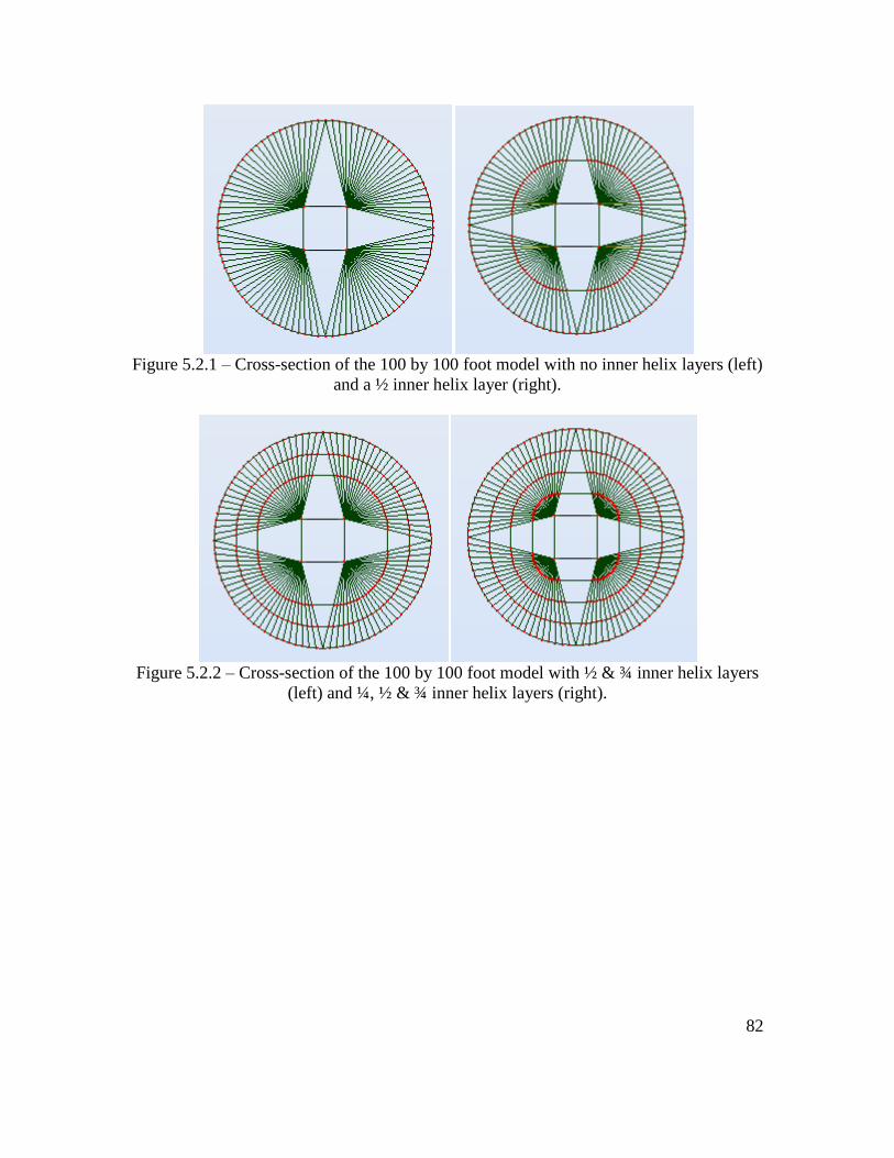
82
Figure 5.2.1 – Cross-section of the 100 by 100 foot model with no inner helix layers (left)
and a ½ inner helix layer (right).
Figure 5.2.2 – Cross-section of the 100 by 100 foot model with ½ & ¾ inner helix layers
(left) and ¼, ½ & ¾ inner helix layers (right).

83
Figure 5.2.5 – Side views of the 100 by 100 foot models, listed from top: No inner helix
layer, ½ inner helix layer, ½ & ¾ inner helix layers and ¼, ½, & ¾ inner helix layers.

84
Figure 5.2.4 – Cross-section of the 65 by 130 foot model with no inner helix layers (left)
and a ¾ inner helix layer (right).
Figure 5.2.5 – Cross-section of the 65 by 130 foot model with ¾ & ⅞ inner helix layers
(left) and ⅜, ¾ & ⅞ inner helix layers (right).

85
Figure 5.2.6 – Side views of the 65 by 130 foot models, listed from top: No inner helix
layer, ¾ inner helix layer, ¾ & ⅞ inner helix layers and ⅜, ¾ & ⅞ inner helix layers.

86
The strength of adding the inner helix layers lies in the fact that the load is
distributed in the layers, rather than all in the one outer helix. To continue the analysis,
the best performing bridge in this section will be further analyzed using the member
section steel calculations that can be performed in Robot.
The 65 by 130 foot radius model with the ¾ and ⅞ inner helix had the lowest
maximum dead load deflection in the previous analysis. Using this model and running
the steel design calculations shows that approximately the same percentage of members
do not pass the standards set forth in ANSI/AISC 360-05, which was about 50% for the
65 by 130 foot model with no inner helix. The exaggerated deflected shapes are shown
in the figures below.
Figure 5.2.7 – Exaggerated deflected cross-section of 65 by 130 foot model with ¾ and ⅞
inner helix layers.

87
Figure 5.2.8 – Exaggerated deflected side view of the 65 by 130 foot model with ¾ and ⅞
inner helix layers.
It can be seen in the deflected shape figures that the bridge is still deflecting in much the
same way it was in the previous analyses. Though the magnitudes of the deflections are
certainly lower, the ends are still thin and clearly susceptible to shear. The top helix still
bows out and sinks, while the bottom helix sinks inward towards itself due to its own
weight. The main problem is still the weakness in the way the deck is connected to the
helix, which causes the structure to sag considerable under its own weight. If the helix
was supported (connected to the deck) directly from below, it’s self-weight would be
distributed into that support, but that is not the case with this design, as the model is
supported from the sides only, which is the biggest concern that must be addressed
moving forward.
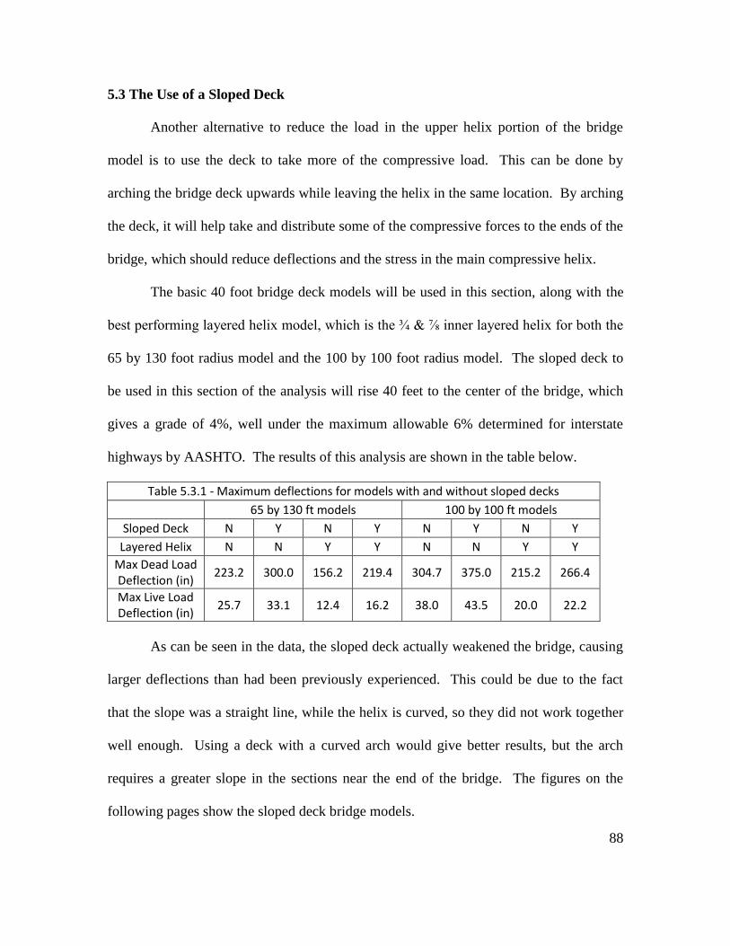
88
5.3 The Use of a Sloped Deck
Another alternative to reduce the load in the upper helix portion of the bridge
model is to use the deck to take more of the compressive load. This can be done by
arching the bridge deck upwards while leaving the helix in the same location. By arching
the deck, it will help take and distribute some of the compressive forces to the ends of the
bridge, which should reduce deflections and the stress in the main compressive helix.
The basic 40 foot bridge deck models will be used in this section, along with the
best performing layered helix model, which is the ¾ & ⅞ inner layered helix for both the
65 by 130 foot radius model and the 100 by 100 foot radius model. The sloped deck to
be used in this section of the analysis will rise 40 feet to the center of the bridge, which
gives a grade of 4%, well under the maximum allowable 6% determined for interstate
highways by AASHTO. The results of this analysis are shown in the table below.
Table 5.3.1 - Maximum deflections for models with and without sloped decks
65 by 130 ft models 100 by 100 ft models
Sloped Deck N Y N Y N Y N Y
Layered Helix N N Y Y N N Y Y
Max Dead Load Deflection (in)
223.2 300.0 156.2 219.4 304.7 375.0 215.2 266.4
Max Live Load Deflection (in)
25.7 33.1 12.4 16.2 38.0 43.5 20.0 22.2
As can be seen in the data, the sloped deck actually weakened the bridge, causing
larger deflections than had been previously experienced. This could be due to the fact
that the slope was a straight line, while the helix is curved, so they did not work together
well enough. Using a deck with a curved arch would give better results, but the arch
requires a greater slope in the sections near the end of the bridge. The figures on the
following pages show the sloped deck bridge models.

89
Figure 5.3.1 – Cross-section of the 65 by 130 foot radius model with the sloped deck.
Figure 5.3.2 – Side view of the 65 by 130 foot radius model with the sloped deck.

90
Figure 5.3.3 – Cross-section of the 100 by 100 foot radius model with the sloped deck.
Figure 5.3.4 – Cross-section of the 100 by 100 foot radius model with the sloped deck.

91
5.4 Bracing the Helix Structure to Reduce Dead Load Deflections
Due to the manner in which every variation of the helix shaped bridge models
have deflected, it is clear that the pure helix shape will require some structural
modification in order to pass the more stringent tests. The main problem is the that the
weight of the outer helix structure sags significantly under its own self-weight, because of
the way it is connected to the deck, which has proven to be not strong enough to support
the structure without significant deflections. This problem is made clear in the figure
below, which shows the 40 foot sections numbered 8 through 18 for the 100 by 100 foot
radius model.
Figure 5.4.1 – Exaggerated deflected shape of sections 8 through 18 of the 100 by 100
foot radius model.
It is extremely clear in the image above that the outer helix structure is sinking severely
under its own weight. This must be addressed before the members will begin to pass any
of the tests performed in the calculations for ANSI/AISC 360-05, because the bridge is
sagging so much under its own weight that the members are taking higher forces than if
they were supported and connected in a more efficient manner. The next step is to
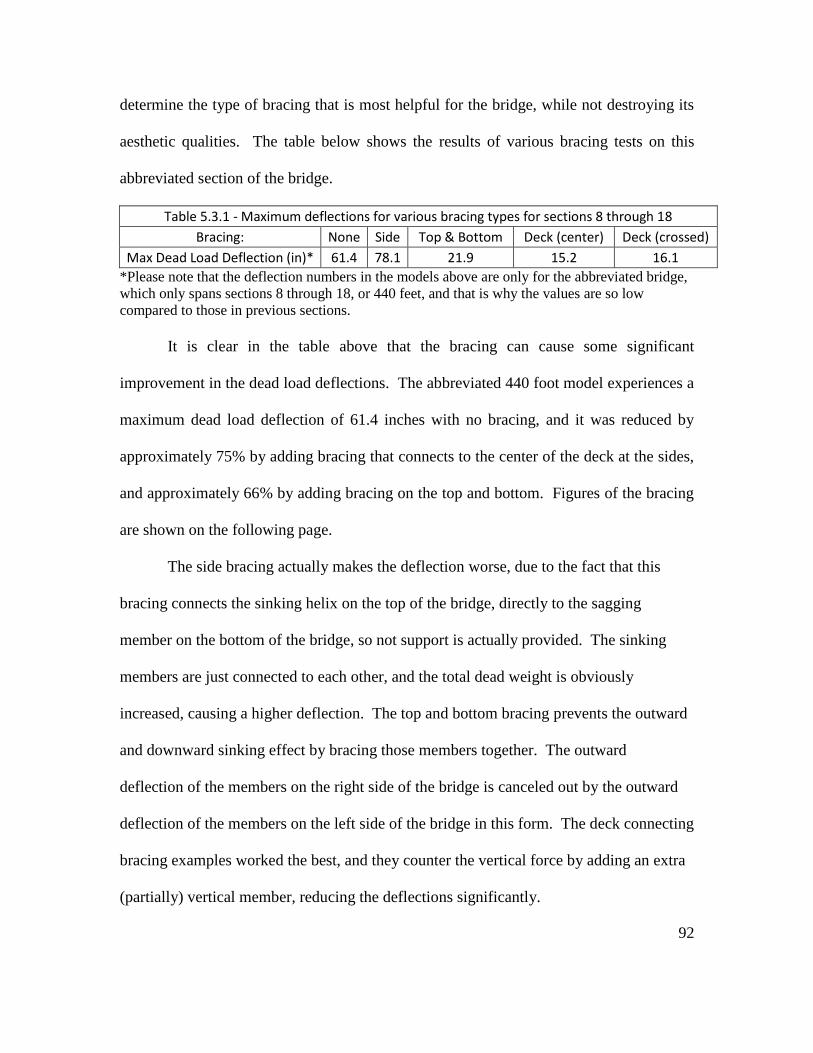
92
determine the type of bracing that is most helpful for the bridge, while not destroying its
aesthetic qualities. The table below shows the results of various bracing tests on this
abbreviated section of the bridge.
Table 5.3.1 - Maximum deflections for various bracing types for sections 8 through 18
Bracing: None Side Top & Bottom Deck (center) Deck (crossed)
Max Dead Load Deflection (in)* 61.4 78.1 21.9 15.2 16.1
*Please note that the deflection numbers in the models above are only for the abbreviated bridge,
which only spans sections 8 through 18, or 440 feet, and that is why the values are so low
compared to those in previous sections.
It is clear in the table above that the bracing can cause some significant
improvement in the dead load deflections. The abbreviated 440 foot model experiences a
maximum dead load deflection of 61.4 inches with no bracing, and it was reduced by
approximately 75% by adding bracing that connects to the center of the deck at the sides,
and approximately 66% by adding bracing on the top and bottom. Figures of the bracing
are shown on the following page.
The side bracing actually makes the deflection worse, due to the fact that this
bracing connects the sinking helix on the top of the bridge, directly to the sagging
member on the bottom of the bridge, so not support is actually provided. The sinking
members are just connected to each other, and the total dead weight is obviously
increased, causing a higher deflection. The top and bottom bracing prevents the outward
and downward sinking effect by bracing those members together. The outward
deflection of the members on the right side of the bridge is canceled out by the outward
deflection of the members on the left side of the bridge in this form. The deck connecting
bracing examples worked the best, and they counter the vertical force by adding an extra
(partially) vertical member, reducing the deflections significantly.
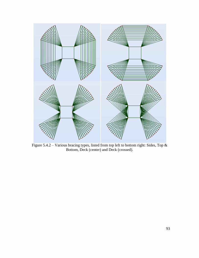
93
Figure 5.4.2 – Various bracing types, listed from top left to bottom right: Sides, Top &
Bottom, Deck (center) and Deck (crossed).
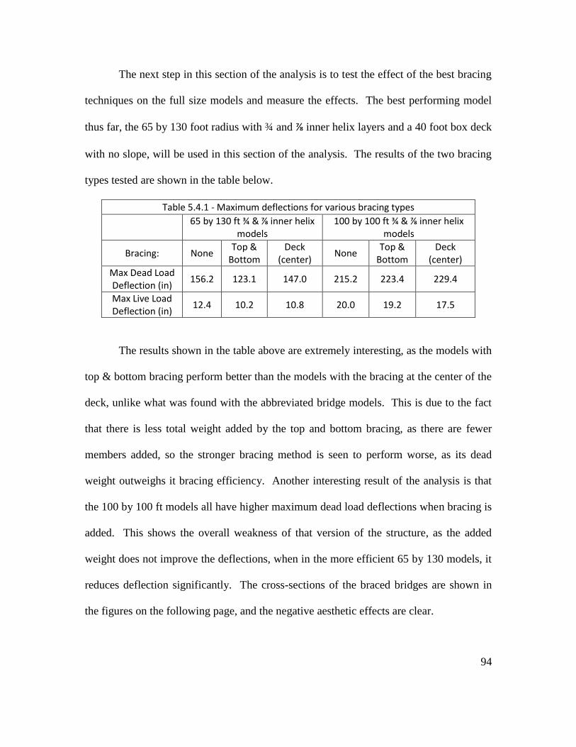
94
The next step in this section of the analysis is to test the effect of the best bracing
techniques on the full size models and measure the effects. The best performing model
thus far, the 65 by 130 foot radius with ¾ and ⅞ inner helix layers and a 40 foot box deck
with no slope, will be used in this section of the analysis. The results of the two bracing
types tested are shown in the table below.
Table 5.4.1 - Maximum deflections for various bracing types
65 by 130 ft ¾ & ⅞ inner helix
models 100 by 100 ft ¾ & ⅞ inner helix
models
Bracing: None Top &
Bottom Deck
(center) None
Top & Bottom
Deck (center)
Max Dead Load Deflection (in)
156.2 123.1 147.0 215.2 223.4 229.4
Max Live Load Deflection (in)
12.4 10.2 10.8 20.0 19.2 17.5
The results shown in the table above are extremely interesting, as the models with
top & bottom bracing perform better than the models with the bracing at the center of the
deck, unlike what was found with the abbreviated bridge models. This is due to the fact
that there is less total weight added by the top and bottom bracing, as there are fewer
members added, so the stronger bracing method is seen to perform worse, as its dead
weight outweighs it bracing efficiency. Another interesting result of the analysis is that
the 100 by 100 ft models all have higher maximum dead load deflections when bracing is
added. This shows the overall weakness of that version of the structure, as the added
weight does not improve the deflections, when in the more efficient 65 by 130 models, it
reduces deflection significantly. The cross-sections of the braced bridges are shown in
the figures on the following page, and the negative aesthetic effects are clear.

95
Figure 5.4.3 – Cross-sections of the 65 by 130 foot models with top & bottom bracing
(left) and center deck bracing (right).
Figure 5.4.4 – Cross-sections of the 100 by 100 foot models with top & bottom bracing
(left) and center deck bracing (right).

96
The top and bottom bracing clearly improved the most efficient model
significantly. The best performing model to this point in the analysis now contains the
following variables:
65 by 130 foot radii
22.5 inch diameter circular steel members with a yield strength of 36 ksi
40 foot thick box deck with no slope
¾ and ⅞ inner helix layers
Top and bottom bracing
When the steel section calculations are performed on this model, the results show that
approximately 45% of the members are still not passing the parameters set forth in
ANSI/AISC 360-05. Although the shape has been optimized, there are still significant
issues pertaining to the individual members, which means that the next step in the
analysis must be to alter the member sections and materials in order to pass the code
standards. An isometric view of the bridge listed above can be found on the following
page.

97
Figure 5.4.5- Isometric view of the most efficient helix bridge shape with bracing.

98
6.0 Optimizing the Individual Steel Members
The individual steel members for the most efficient helix shaped model are not
strong enough to pass the tests performed using the code standards in ANSI/AISC 360-
05. Although the dead load deflections have been reduced significantly to manageable
levels (10 feet of deflection over a 2000 foot span can be constructed for using pre-
cambering techniques), they are still causing enough deflections so that the members are
failing. The live load deflections have also been reduced to approximately 10 inches,
which is well under the allowable maximum of 30 inches for a 2000 foot span, but the
model is still unable to pass the more stringent tests, and a second order analysis has not
even been performed to this point.
The first step in improving the strength of the steel is to increase its yield strength.
This will not change the live or dead load deflections in any way, but it will improve the
performance of the individual members against the steel section code tests calculated by
Robot for ANSI/AISC 360-05. This is because the deflections are dependent on the
modulus of elasticity of the steel, which is 29 x 106 psi for all steel, as discussed in an
earlier section. The individual member strength is dependent on the yield strength of the
steel, as each member is individually checked based on its material and size properties.
The previous most efficient model was created using 22.5 inch solid circular
members with a yield strength of 36 ksi. Approximately 45% of the members could not
pass the standards calculated for in ANSI/AISC 360-05. When the material is changed to
a higher strength steel, a vast improvement can be seen. The maximum available yield
strength for the materials available in Robot is 105 ksi, which is often used in the cables
of long span bridges. When the members are switched to the 105 ksi steel, only about

99
20% of them fail to pass the ANSI/AISC 360-05 calculations, meaning that 20% of them
have an efficiency rating of greater than 1. This is a significant improvement, and the
105 ksi steel will be used as the material for the models for the rest of the analysis. 105
ksi steel is typically only used in high strength cables, but it will be used for the duration
of this analysis, though the final models will be rechecked using steel using lower yield
strengths. Though the steel strength has been improved, there is still clearly a major issue
with the individual member failures against the code calculations, so the next step in the
analysis will be to optimize the member section shapes.

100
6.1 Optimizing the Member Sections
In the previous sections, the shape of the helix bridge was optimized in order to
reduce dead load deflections down to a manageable value. The next step is to further
reduce the deflections by optimizing the member sections. The member section used
until this point in the analysis was a 22.5 inch diameter solid circle in cross-section, but
this is clearly not strong enough to pass the next levels of the analysis. Various members
sections were tested using the most efficient bridge model to this point in the analysis,
and the results are shown in the tables below:
Table 6.1.1 - Maximum deflections for various circular section types
Diameter (in) 22.5 24 24 48 48
Wall Thickness (in) Solid Solid 6 Solid 12
Cross-sectional Area (in2) 397.6 452.4 339.3 1809.6 1357.2
Max Dead Load Deflection (in) 123.1 122.0 120.2 113.5 112.6
Percentage of members failing ANSI/AISC Code tests
20% 20% 10% 0.60% 0.60%
Table 6.1.2 - Maximum deflections for various square section types
Width & Height (in) 24 24 48 48
Wall Thickness (in) Solid 6 Solid 12
Cross-sectional Area (in2) 576.0 432.0 2304.0 1728.0
Max Dead Load Deflection (in) 119.9 118.4 112.4 111.6
Percentage of members failing ANSI/AISC Code tests
10% 6% 0.50% 1.50%
Both circular and square sections were tested, as shown in the tables above. The best
overall performance came from the largest square cross-sections, which had the lowest
dead load deflections, and the lowest percent of member failures. The first interesting
point of note is that increasing the member cross-section size does automatically imply
significantly better results. Though the dead load deflections went down when the

101
diameters and square sides were doubled, they did not decrease very much. This simply
shows that a balance between increasing the size and decreasing the self-weight needs to
be found. Another observation from the results of these calculations is that the non-solid
member performed noticeably better than their solid counterparts. The members listed in
the table with a “wall thickness” are pipes or tubes, which have hollow centers. This is a
way to find a balance between decreasing the self-weight and designing against buckling.
As discussed in an earlier section, a member with a higher of gyration is less likely to
buckle. By using a tube cross-section, the member will have a lower self-weight than a
solid member of the same outer cross-section dimensions, but a higher radius of gyration
than a solid member with the same cross-sectional area. By using this balance, a more
efficient member section design can be found.
Using the member section analysis that was just discussed, the next step is to see
if all of the members need to be the same section. It is clear that forces distribute
differently in members throughout the bridge, as the members making up the main
compression helix take a much greater axial load than any other members in the bridge.
For example, in the model using a tube cross-section with a square side of 24 inches and
a wall thickness of 6 inches, the member with the highest axial force is the member in the
main outer helix that connects the first section of the bridge to the pin connection at the
end. The axial force in this member is 32,248.75 kips. A member with very little force
can be found at the 160 feet from the center of the bridge on top level of the deck, and it
experiences an axial force of 0.96 kips. The difference is massive, and this leads into the
next part of the optimization. The figures on the next page show the highest and lowest
stressed member on the bridge.

102
Figure 6.1.1 – The member with the lowest axial force (highlighted in red).
Figure 6.1.2 – The members with the highest axial forces (highlighted in red).

103
Rather than change the section of each member individually, two of the earlier
member sections will be used in one design to test the effect of increasing the sections
where the forces are greatest. The outer helix experiences the most force, and therefore is
given the 48 inch square tube cross section with a wall thickness of 12 inches, while
every other member in the bridge will be the smaller tube cross-section, the 24 inch
square with a wall thickness of 6 inches. When the analysis is run with this combination,
the change in the results is drastic. The maximum dead load deflection is reduced to 72.1
inches. Out of the 1808 of the members in the bridge, 12 of them have efficiency ratios
of greater than 1 in the ANSI/AISC 360-05 steel section calculations, which is still
approximately 0.70%, but all of the members that do not pass code are 24 inch tubes, the
entire outer helix passes the member tests.
In order to get all of the members to pass the code tests, they are individually
found and switched to 48 inch square tube cross-sections. The failing members were the
24 inch cross-sectional tubes that were closest to the supports, where the forces were
most concentrated. When these members are switched to 48 inch square tubes, every
member in the model passes the ANSI/AISC 360-05 steel section calculations. These
calculations only cover the first order dead load case, and the next step is to get the model
to pass the second order analysis.

104
6.2 Failure in the Second Order Analysis
The second order non-linear analysis tests the model by adding the load to the
bridge in increments. The standard procedure is to test the bridge in five increments,
20%, 40%, 60%, 80% and 100%, which Robot performs through its non-linear analysis
option. This test most importantly tests for major changes in shape that are not recovered
from when the design is loaded in separate increments, and a failure of the second order
analysis implies that the bridge model is most likely experiencing buckling.
Using the model that passes the first order tests and running a second order
analysis shows that the model is not strong enough. The model only makes it through the
first two iterations (20 % and 40%) before the analysis begins to show failure. When the
analysis is performed by Robot, it loads and unloads in the previously stated increments,
if the model passes, the deflection values for the second order analysis will be less than
those of the first order analysis. If it fails, it is implied that greater deflections were being
experienced. In the analysis itself, a graph is shown, and when each iteration is run, the
graph will converge or an error will appear after multiple failures: “No convergence of
nonlinear problem”. Because this error appears after only two iterations of five, it is clear
that this model is not nearly strong enough to pass the second order tests.
Further optimization of the shape is clearly required, as increasing the member
sections infinitely is not a reasonable solution. The exaggerated deflected shape of the
model that passes the first order tests is shown on the following page, and a closer look
into that shape is vital to the next phase of the optimization.

105
Figure 6.2.1 – Cross-section of the exaggerated deflected shape that passes the first order
analysis, but fails the second order analysis.
Figure 6.2.2 – Side view of the exaggerated deflected shape that passes the first order
analysis, but fails the second order analysis.
It is clear from the figures above that the bridge is deflecting in only one of the two ways
that had been experienced in earlier analyses. The sagging or sinking that was being
experienced in the outer helix due the dead load has been essentially eliminated by the
bracing and the increase in the strength of the outer helix members. The other way in
which the bridge is deflecting had not changed, as there is clearly shear being
106
experienced near the ends of the bridge. This is still due to the excessive thinness of the
model towards its ends, a problem that hasn’t been addressed to this point. It can be seen
in the side-view that the bridge still deflects significantly at the ends, and barely at all
towards the strong center. This is still due to the fact that the helix rises at its highest
point above the bridge at the center, easily taking the high tension and compression
forces, but they are distributed to the ends of the bridge into an area that is very thin and
extremely susceptible to shear. The optimization process up to this point maintained the
helix shape with only minor bracing, but the helix shape is clearly not strong enough to
resist the shear at the ends of the bridge, so further modifications must be made.

107
7.0 Optimizing Alternative Designs to Pass Second and Third Order Analyses
Though the basic helix structure was able to pass the first order analysis tests, it is
unable to pass the second and third order tests that are required for real-world usability.
An alternative design will be required in order to pass these more stringent non-linear
tests, and it clearly must address the main problem with the basic helix design, which is
shear at the ends of the bridge. Another equally important requirement is that the bridge
design must maintain the aesthetic integrity of the original helix design. The main
purpose of the analysis is to create a bridge that performs to standards structurally, but
also utilizes the aesthetic benefits of the curved helix shape, so any alternative design
must maintain these ideals.

108
7.1 Alternative Approaches to Reduce Shear: 2-D Line Models
The main problem to this point in the analysis has been determined to be the shear
forces experienced in the bridge models near the supports. The deflections experienced
by the bridge as a whole have been seen mostly in the ends of the bridge, with only minor
deflections in center sections, were the model is strongest. This is dues to the thinness of
the bridge, and the lack of strength that goes along with it, at the ends of the bridge near
the supports. To further study, and try to negate the shear forces, a serious if line models
will be analyzed.
The line models look the same as the previous bridges from a side-view in the y-z
plane (along the 2000 foot length), but in the x-z plane, they are just a straight line,
instead of the earlier full-radius models. These 2-D models obviously aren’t capable of
carrying traffic, but studying the shape will help with the progression of the analysis.
Two variations are used in the following analysis. The first is the use of diagonals in the
models, as pictured on the following pages. The other is to use the parabolic moment
equation to design the outer structure of the bridge, rather than the helical sine curve.
The bridge outer “helix” structure follows the parabolic moment equation discussed
earlier, which is the most efficient shape for distributing the load in the y-z plane.
Table 7.1.1 - Maximum deflections for 2-D line model variations
Helical side-view models Parabolic side-view models
100 foot height 120 foot height 100 foot height 120 foot height
Diagonals N Y N Y N Y N Y
Max Dead Load Deflection (in)
137.0 105.9 132.5 79.5 115.3 94.4 107.2 71.4
As can be seen in the results above, adding diagonals and using the parabolic equation
help reduce the dead load deflections drastically. The use of the parabolic equation

109
strengthens the ends of the bridge near the support, as the outer structure rises quicker
towards the middle. For the 100 foot height helix shaped bridge, the first section rises
6.28 feet from the end support to the start of the second section. For the 100 foot
parabolic shaped bridge, the first section rises 7.84 feet, which strengthens the ends of the
bridge, where the shear is greatest. The table on the following page shows the Z-values
of the outer structure for the four line models tested on the previous page. As can be seen
in the table, the parabolic shape increases towards its maximum height at the center
(y=1000 feet) from the edges of the bridge (y=0 feet) much quicker for the parabolic
shaped models than for the helix shaped models. This increased rise from the edges
greatly reduces the deflections, as the helix shaped 100 foot height model has a maximum
dead load deflection of 137.0 inches, while the 100 foot height parabolic shaped model
has a maximum dead load deflection of 115.3 inches, which is almost 20% less, a major
reduction. All of the 2-D models used 48 inch square tubes with 12 inch wall thickness
members (in cross-section) for the outermost part of the structure, while the rest of the
connecting members are 24 inch square tubes in cross section with 6 inch wall
thicknesses.
The next part of the analysis is to look at the effect of the diagonals in the 2-D line
models. As can be seen in the results on the previous page, the diagonals drastically
reduce the maximum dead load deflections in each model. This is due to the fact that the
diagonals help take and distribute the shear forces at the ends of the bridge. This increase
in structural strength is readily apparent for the 2-D line models, but it must be noted that
diagonals will be troublesome to use in a 3-D model, while the diagonals also take away
from the models aesthetically. Images of the 2-D line models can be found on the
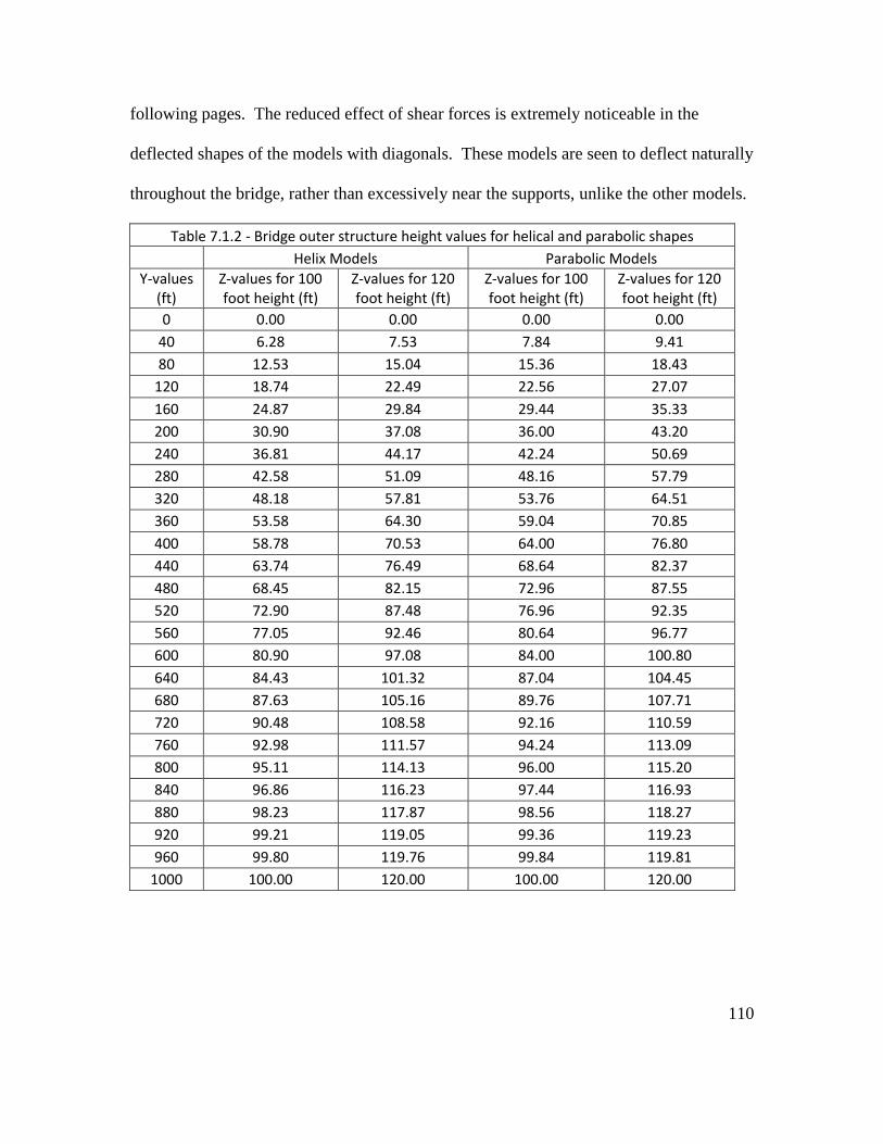
110
following pages. The reduced effect of shear forces is extremely noticeable in the
deflected shapes of the models with diagonals. These models are seen to deflect naturally
throughout the bridge, rather than excessively near the supports, unlike the other models.
Table 7.1.2 - Bridge outer structure height values for helical and parabolic shapes
Helix Models Parabolic Models
Y-values (ft)
Z-values for 100 foot height (ft)
Z-values for 120 foot height (ft)
Z-values for 100 foot height (ft)
Z-values for 120 foot height (ft)
0 0.00 0.00 0.00 0.00
40 6.28 7.53 7.84 9.41
80 12.53 15.04 15.36 18.43
120 18.74 22.49 22.56 27.07
160 24.87 29.84 29.44 35.33
200 30.90 37.08 36.00 43.20
240 36.81 44.17 42.24 50.69
280 42.58 51.09 48.16 57.79
320 48.18 57.81 53.76 64.51
360 53.58 64.30 59.04 70.85
400 58.78 70.53 64.00 76.80
440 63.74 76.49 68.64 82.37
480 68.45 82.15 72.96 87.55
520 72.90 87.48 76.96 92.35
560 77.05 92.46 80.64 96.77
600 80.90 97.08 84.00 100.80
640 84.43 101.32 87.04 104.45
680 87.63 105.16 89.76 107.71
720 90.48 108.58 92.16 110.59
760 92.98 111.57 94.24 113.09
800 95.11 114.13 96.00 115.20
840 96.86 116.23 97.44 116.93
880 98.23 117.87 98.56 118.27
920 99.21 119.05 99.36 119.23
960 99.80 119.76 99.84 119.81
1000 100.00 120.00 100.00 120.00

111
Figure 7.1.2 – Side-view of the 100 foot height helix 2-D model and exaggerated
deflected shape. The equation for the outer top (and bottom) members follows the
previously discussed sine curve, and severe shear effects are noticeable.
Figure 7.1.3 – Side-view of the 100 foot height parabolic 2-D model with diagonals and
exaggerated deflected shape. The equation for the outer top (and bottom) members
follows the previously discussed parabolic moment equation, and shear effects are
negligible, the bridge sags naturally.
Figure 7.1.3 – Isometric view of the 100 foot height parabolic 2-D model with diagonals
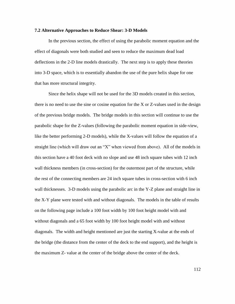
112
7.2 Alternative Approaches to Reduce Shear: 3-D Models
In the previous section, the effect of using the parabolic moment equation and the
effect of diagonals were both studied and seen to reduce the maximum dead load
deflections in the 2-D line models drastically. The next step is to apply these theories
into 3-D space, which is to essentially abandon the use of the pure helix shape for one
that has more structural integrity.
Since the helix shape will not be used for the 3D models created in this section,
there is no need to use the sine or cosine equation for the X or Z-values used in the design
of the previous bridge models. The bridge models in this section will continue to use the
parabolic shape for the Z-values (following the parabolic moment equation in side-view,
like the better performing 2-D models), while the X-values will follow the equation of a
straight line (which will draw out an “X” when viewed from above). All of the models in
this section have a 40 foot deck with no slope and use 48 inch square tubes with 12 inch
wall thickness members (in cross-section) for the outermost part of the structure, while
the rest of the connecting members are 24 inch square tubes in cross-section with 6 inch
wall thicknesses. 3-D models using the parabolic arc in the Y-Z plane and straight line in
the X-Y plane were tested with and without diagonals. The models in the table of results
on the following page include a 100 foot width by 100 foot height model with and
without diagonals and a 65 foot width by 100 foot height model with and without
diagonals. The width and height mentioned are just the starting X-value at the ends of
the bridge (the distance from the center of the deck to the end support), and the height is
the maximum Z- value at the center of the bridge above the center of the deck.
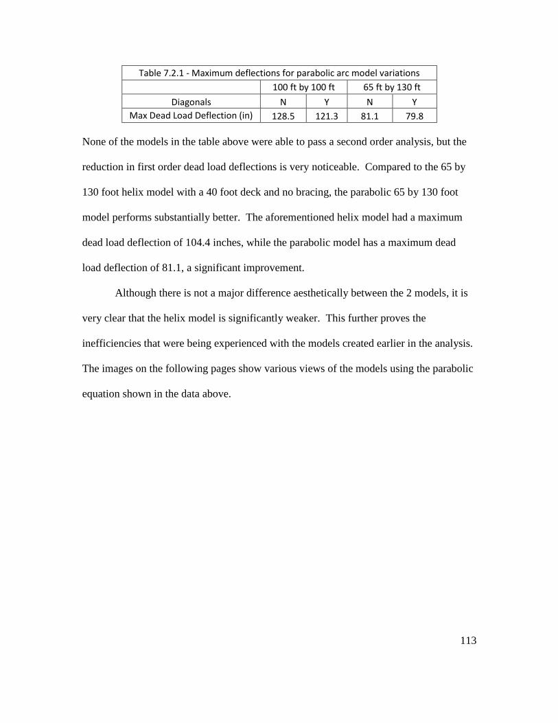
113
Table 7.2.1 - Maximum deflections for parabolic arc model variations
100 ft by 100 ft 65 ft by 130 ft
Diagonals N Y N Y
Max Dead Load Deflection (in) 128.5 121.3 81.1 79.8
None of the models in the table above were able to pass a second order analysis, but the
reduction in first order dead load deflections is very noticeable. Compared to the 65 by
130 foot helix model with a 40 foot deck and no bracing, the parabolic 65 by 130 foot
model performs substantially better. The aforementioned helix model had a maximum
dead load deflection of 104.4 inches, while the parabolic model has a maximum dead
load deflection of 81.1, a significant improvement.
Although there is not a major difference aesthetically between the 2 models, it is
very clear that the helix model is significantly weaker. This further proves the
inefficiencies that were being experienced with the models created earlier in the analysis.
The images on the following pages show various views of the models using the parabolic
equation shown in the data above.

114
Figure 7.2.1 – Cross-sections of the 100 foot width by 100 foot height (left) and 65 foot
width by 130 foot height (right) models that follow the parabolic moment equation.
Figure 7.2.2 – Side-views of the 65 foot width by 100 foot height parabolic models with
and without diagonals. The outer curve follows the parabolic moment equation.
Figure 7.2.3 – Top views of the 65 foot width by 100 foot height parabolic models with
and without diagonals. The outer curves follow a straight line path from above.

115
Figure 7.2.4 – Side-views of the exaggerated deflected shapes of the 65 foot width by 100
foot height parabolic models with and without diagonals. As can be seen, the model with
the diagonals deflects more naturally due to gravity as the shear forces at the ends are
better resisted
Figure 7.2.5 – Isometric view of the 65 foot width by 100 foot height parabolic model
without diagonals.

116
Figure 7.2.6 - Isometric view of the 65 foot width by 100 foot height parabolic model
with diagonals.
As can be seen in the figures, the cross-section no longer makes the shape of the
aesthetically desired circle or ellipse. It is also clear that the diagonals severely impact
the aesthetics of the bridge design, giving them an almost cluttered feel.
To show the differences between the helix shaped models and the parabolic
shaped models that follow straight line paths from above, a series of images will be used
to display the differences. In general, they have the same overall dimensions and can fit
into the same envelope, but the parabolic model (65 by 130 with no diagonals) has a
maximum dead load deflection of 81.1 inches, while the 65 foot by 130 foot helix model
with no bracing or layering deflects a maximum of 104.4 inches, or about 25% more.

117
Figure 7.2.7 – Cross-sections of the parabolic (left) and helical (right) shaped models.
Figure 7.2.8 – Side-views of the parabolic (top) and helix (bottom) shaped models.
Figure 7.2.9 – Top-views of the parabolic (top) and helix (bottom) shaped models.
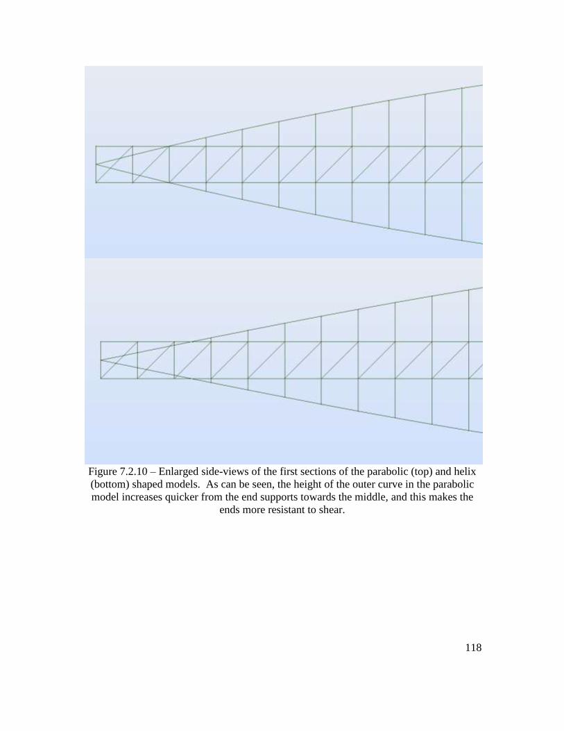
118
Figure 7.2.10 – Enlarged side-views of the first sections of the parabolic (top) and helix
(bottom) shaped models. As can be seen, the height of the outer curve in the parabolic
model increases quicker from the end supports towards the middle, and this makes the
ends more resistant to shear.

119
Figure 7.2.11 – Enlarged top-views of the first sections of the parabolic (top) and helix
(bottom) shaped models. As can be seen, the straight line model takes a direct path to the
supports, while the helix is perpendicular to the supports at the ends. This curve causes
the helix to “bow-out”, as discussed in earlier sections, causing significant deflections.

120
Figure 7.2.12 – Cross-sections of the deflected shapes of the helix (top) and parabolic
(bottom) shaped models. The effects of the outward pushing and sagging are clearly
visible in the helix model (top), while they are not seen in the parabolic model below.

121
Figure 7.2.13 – Side-views of the exaggerated deflected shapes of the parabolic (top) and
helix (bottom) models. The effects of shear and the excessive deflection of the outer
helix are extremely noticeable in the helix model (bottom), but are clearly mitigated in
the parabolic model (top).
The major differences between the parabolic and helix shaped models are very clear in
the images shown on the previous pages. The parabolic shaped models are stronger for
two primary reasons. The first is the fact that the parabolic shape is better at taking the
shear forces at the ends of the bridge. The shear force is better distributed because the
bridge rises higher from the ends, causing the bridge to deflect less due to shear and have
a more natural deflected shape. The force at the supports is an upward one, so the
internal shear force near the near the ends of the bridge is better distributed when the
bridge it taller near the ends. The other major difference between the two models is the
fact that the parabolic model also takes a straight line path from support to support when
viewed from above (the change of the of the X-values of the points on the outer parabolic
structure is constant and equal across the entire span, creating a straight line). The curve
in the helix model causes the compressive force to push the helix both upwards and
outwards, rather than the compressive force in the straight line model, which only creates
an upward push in the top outer support structure. The outward push in the curved helix
122
model further exaggerates the sagging of the helix shaped models, as the outward push
combined with gravity causes the sagging. In the parabolic shaped straight line model,
the upward push caused from the compression counteracts the sagging effect, which
reduces the effects of the shear forces and the defections.
The parabolic shaped models with straight lines connecting the supports across
the bridge still do not pass the second order analysis tests. This is still due to the fact that
there is excessive bending and buckling of the members near the end due to the fact the
models are too thin near the supports. The next strategy is to add a third arch to the
bridge, down the center, to further support the bridge near the supports. This triple
parabolic arch model (with full diagonals in each arch and bracing to support the center
arch) is created first without a deck or roadway of any kind, in order to first study the
visual effects and the structural strength improvements, before creating a full model. The
connecting members simply meet along a straight line in the center of the model, as
shown in the images on the following pages.

123
Figure 7.2.14 – Cross-section of the triple parabolic arch model.
Figure 7.2.15 – Side-view of the triple parabolic arch model.
Figure 7.2.16 – Top-view of the triple parabolic arch model.

124
Figure 7.2.16 – Top-view of the triple parabolic arch model.
This model passes the second order analysis performed by Robot. Although this is an
overall step forward in the analysis process, as can be seen in the images, the model has
an extremely cluttered visual feel to it, which is not aesthetically desirable. The third
arch would also require major modifications to the deck system, as a median would need
to be built at the center of the bridge for traffic flow purposes. This would require a
wider deck, and new way to distribute the lanes (the current 3 lanes in each direction
model would not work because of the median). Due to these factors, this model will not
be pursued any further, and a new alternative will be studied in the next section.

125
7.3 Alternative Designs: Arching the Deck
The problem to this point in the analysis has been determined to be the weakness
in the in the upper portion of the helix (or parabola) near the ends of the deck. These
members are bending excessively and/or buckling, and this is causing the models to fail
the second order analyses being performed by Robot. The most simply way to fix this
issue is to add additional support to the compressive (upper) part of the structure, and one
way to do this is to use the deck to take some of the compressive force end distribute it to
the ends. This is a similar idea to the triple parabolic arch model from the last section,
but an arched deck is now used in lieu of the third parabolic arch.
Because of AASHTO standards, a road cannot have a maximum grade of more
than 6%, which is what the deck must be designed for [21]. The ideal scenario for the
deck would be for it stay within the AASHTO standards, while also following the
parabolic moment equation shape, which has proven to be the strongest arch shape
throughout the analysis. Two different designs will be tested, both of which use an
arched deck to take a compressive force on the top of the bridge.
The first model has a deck which follows the parabolic shape, and the deck sits
entirely above the parabolic support system. Because the slope of a parabolic deck is at a
maximum in the first section from the support, this is the only section that will be at the
maximum 6% grade. The rest of the sections will follow the shape of the arch, leading to
a maximum height at the center of 31.25 feet. The 40 foot deck is added to this value,
giving a maximum height at the center of 71.25 feet above the supports. Because the
ideal total height of the bridge has been proven to be at least 200 feet, the lower tension
supports will reach a maximum depth of 129.75 feet below the supports. This will also

126
require a middle layer connecting the lower tension structure to the upper compression
structure, as the members would have to be too long if they connected directly from the
lower level to the upper.
The second model has a partially straight-sloped, partially parabolic-sloped deck,
which is infused with the upper parabolic compression structure. The height of the
bridge is 100 feet at the center, while it also has a depth of 100 feet, giving it the same
total height of 200 feet. To allow for the top layer of the deck to reach a maximum height
of 100 feet, while also staying within AASHTO standards, the deck will increase at the
maximum 6% grade until it is even with the upper parabolic structure, and then it will
follow the same parabolic arch as the upper structure, fusing the two together. This will
give the deck a desirable height, while also keeping it aesthetically within the parabolic
model shape.
Both deck bridges use 48 inch square tubes with 12 inch wall thicknesses in the
outer compression and tension parabolic arches, as well as in the top most layer of the
deck, while all other members are of the smaller square tube variety. Images of both of
the bridges are found on the following pages.

127
Figure 7.3.1 – Cross-sections of the deck above the arch (left) and the deck infused with
the arch (right) models. Both models have 40 foot wide decks and 60 foot horizontal
radii (or 120 foot total widths).
Figure 7.3.2 – Side-views of the deck above the arch (top) and the deck infused
with the arch (bottom) models.

128
Figure 7.3.3 – Isometric view of the deck above the arch model with member sections
turned on.
Figure 7.3.4 – Isometric view of the deck infused with the arch model with member
sections turned on.

129
As can be seen on the figures on the previous pages, the decks are used with the crossing
parabolic arches to give additional support in compression. This allows for both of these
models to pass the second order analyses performed by Robot, as shown in the table
below.
Table 7.3.1 - Maximum deflections for the arched deck models
Deck above the arches Deck infused with the arches
Max 1st order deflection (in) 124.7 128.3
Max 2nd order deflection (in) 120.9 123.9
Max 3rd order deflection (in) 120.4 Failure
It is clear that the added strength due to the arched deck allows for the models to be
strong enough to pass the tests, although they have ventured extremely far from the
original helix idea (in an aesthetic sense). These models show that a steel bridge can be
built to cross a 2000 foot span, but they do not use any elements of the aesthetically
desirable helix shape, so a final alternative design will be explored in the next section.

130
7.4 Alternative Design: The Double Helix
The designs that have been used to this point in the analysis have used the helix
shape so that it starts at one end of the bridge and does a half turn across the span to
connect at the other side. This “half-helix” shape is used 4 times, and the helix structure
that has been used throughout the analysis is created. It is necessary to use the helix that
only does a half turn over the span because any greater amount of turn would cause the
bridge to have a point of zero height which occurs somewhere along the span besides at
the ends, which will cause immediate structural failure. The highest point of the span
must be at the center, where the strength is needed the most. The problem with the “half-
helix” shape is that its height does not increase quickly enough from the ends of the
bridge as it spans towards the center, which causes the ends to be thin, weak and
susceptible to buckling. One way to improve this is to increase how quickly the height of
the outer structure rises from the ends, towards the center. This was in fact performed
earlier in the analysis, as increasing the overall height of the helix structure causes the
helix to rise quicker from the ends. It was also seen that increasing the height after a
certain point will not help, as the added self-weight eventually causes the structure to
experience greater deflections. A different shape could be used that would increase the
slope of the outer structure as it spans from the ends towards the center, but using a
different arc or parabolic equation would leave the helical design, which is not desired
In order to maintain the helix shape and decrease the shear at the ends of the
bridge, an alternate helix shape will be combined with the existing one. The current
“half-helix” makes one half turn across the span of the bridge, and reaches a maximum
height at the center. The proposed alternative will combine this helix with a “full-helix”

131
or a helical shape that starts at the same zero point, but makes a full turn around the
bridge over the span. It reaches a maximum height at the quarter point of the span, and
has a height of zero at the center. If used without the “half-helix” for support at the
center, failure would be inevitable; as the bridge would have no strength at the point it is
most needed.
The initial combination of the half and full helix uses the following variables:
100 foot by 100 foot radius in cross section for both helixes
40 foot box deck with no slope and a middle level
48 inch square tube with a 12 inch wall thickness for all of the outer helix
members, and the members that connect the three peaks
24 inch square tube with a 6 inch wall thickness for all other members
No inner helix layers
Both helixes are connected to the closest corner of the deck every at 40 foot
section, and are also connected to each other by a member from the ends of the
span until they intersect 1/3 of the way across the span from the nearest end. The
three highest points are connected directly to each other by a members divided
into 40 foot sections.
Using these parameters, the double helix combination passes the first three iterations of
the second order test before non-convergence of the non-linear analysis is found. The
first order maximum dead load deflection is found to be 194.3 inches. The figures on the
following pages show various images of the double helix combination alternative design.
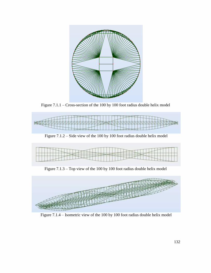
132
Figure 7.1.1 – Cross-section of the 100 by 100 foot radius double helix model
Figure 7.1.2 – Side view of the 100 by 100 foot radius double helix model
Figure 7.1.3 – Top view of the 100 by 100 foot radius double helix model
Figure 7.1.4 – Isometric view of the 100 by 100 foot radius double helix model
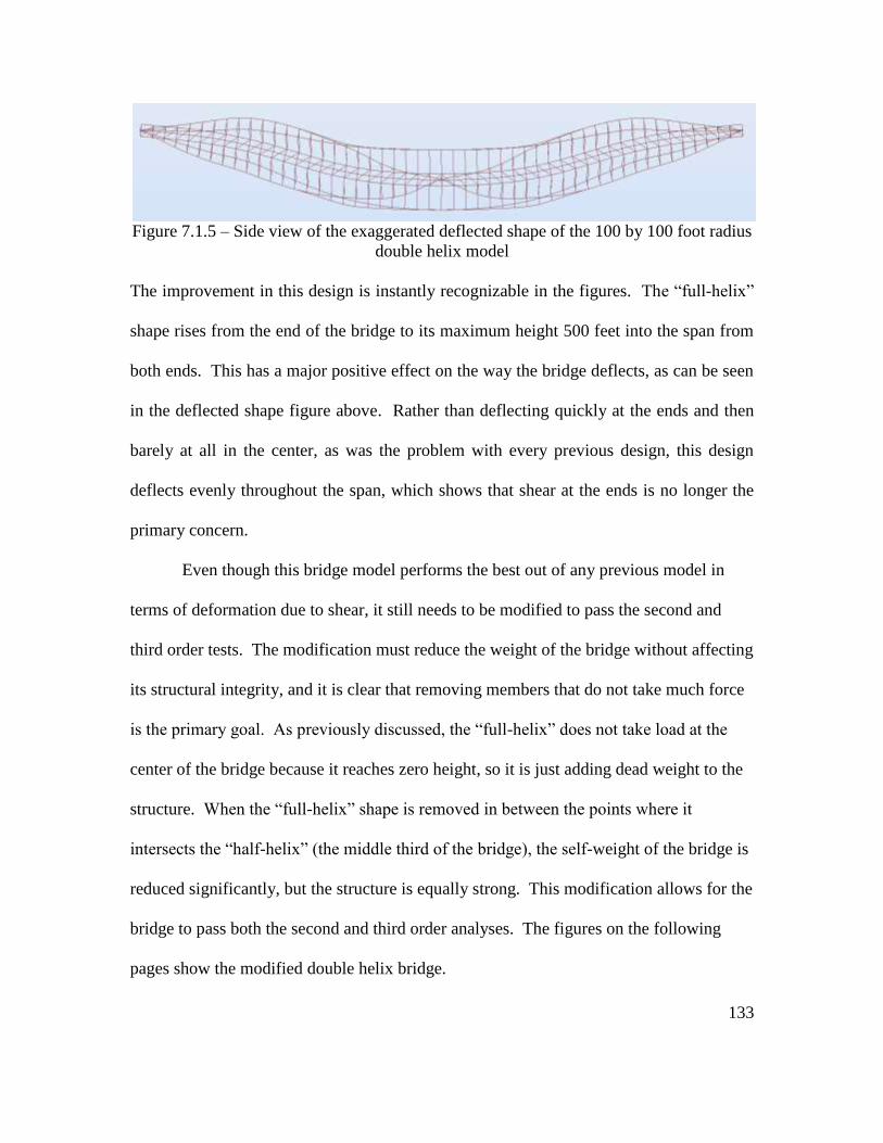
133
Figure 7.1.5 – Side view of the exaggerated deflected shape of the 100 by 100 foot radius
double helix model
The improvement in this design is instantly recognizable in the figures. The “full-helix”
shape rises from the end of the bridge to its maximum height 500 feet into the span from
both ends. This has a major positive effect on the way the bridge deflects, as can be seen
in the deflected shape figure above. Rather than deflecting quickly at the ends and then
barely at all in the center, as was the problem with every previous design, this design
deflects evenly throughout the span, which shows that shear at the ends is no longer the
primary concern.
Even though this bridge model performs the best out of any previous model in
terms of deformation due to shear, it still needs to be modified to pass the second and
third order tests. The modification must reduce the weight of the bridge without affecting
its structural integrity, and it is clear that removing members that do not take much force
is the primary goal. As previously discussed, the “full-helix” does not take load at the
center of the bridge because it reaches zero height, so it is just adding dead weight to the
structure. When the “full-helix” shape is removed in between the points where it
intersects the “half-helix” (the middle third of the bridge), the self-weight of the bridge is
reduced significantly, but the structure is equally strong. This modification allows for the
bridge to pass both the second and third order analyses. The figures on the following
pages show the modified double helix bridge.

134
Figure 7.1.6 – Cross-section of the modified 100 by 100 foot radius double helix model
Figure 7.1.7 – Side view of the modified 100 by 100 foot radius double helix model
Figure 7.1.8 – Top view of the modified 100 by 100 foot radius double helix model
Figure 7.1.9 – Isometric view of the modified 100 by 100 foot radius double helix model

135
Figure 7.1.10 – Side view of the exaggerated deflected shape of the modified 100 by 100
foot radius double helix model
This modified double helix structure passes the second and third order tests performed by
Robot. Even though this design passes all of the appropriate tests, the must be seen if a
more efficient design can be found. The 100 by 100 foot radius was chosen early on in
the optimization process as the most efficient perfect circle cross-section, but this must be
retested. The results are shown in the table below.
Table 7.1.1 - Maximum deflections for modified circular cross-section double helix variations
90 foot radius 100 foot radius 110 foot radius 120 foot radius
Max 1st order deflection (in) 170 150.2 132.8 117
Max 2nd order deflection (in) Failure 149.8 Failure Failure
Max 3rd order deflection (in) Failure 150 Failure Failure
As can be seen in the data table above, the optimal radius is 100 feet for the perfect circle
cross-section. The 90 foot radius does not have a high enough maximum height to resist
its own self-weight, whereas the higher radius models have longer members, which are
more prone to buckling.
To further continue the optimization process, bridge models with varying radii
were tested again with the modified double helix shape. The results of this analysis is
shown in the table on the following page.
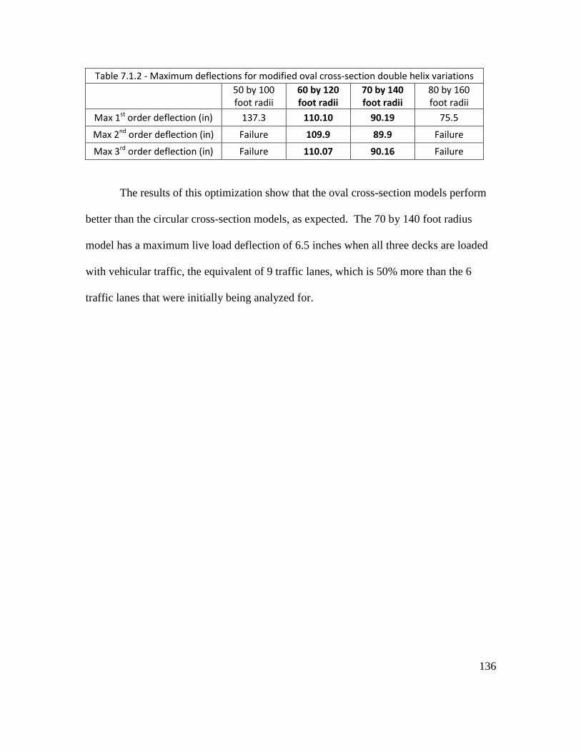
136
Table 7.1.2 - Maximum deflections for modified oval cross-section double helix variations
50 by 100 foot radii
60 by 120 foot radii
70 by 140 foot radii
80 by 160 foot radii
Max 1st order deflection (in) 137.3 110.10 90.19 75.5
Max 2nd order deflection (in) Failure 109.9 89.9 Failure
Max 3rd order deflection (in) Failure 110.07 90.16 Failure
The results of this optimization show that the oval cross-section models perform
better than the circular cross-section models, as expected. The 70 by 140 foot radius
model has a maximum live load deflection of 6.5 inches when all three decks are loaded
with vehicular traffic, the equivalent of 9 traffic lanes, which is 50% more than the 6
traffic lanes that were initially being analyzed for.

137
8. Conclusions and Recommendations
The initial purpose of this study was to explore the use of the helix shape in steel
bridge design. The starting point of the analysis was chosen to be a helix with a flat deck
and a 65 foot radius which was to provide the support over the 2000 foot span. The
maximum live load deflection was 95.7 inches, well over the allowable 30 inches, while
the maximum deflection due to the dead load was an unreasonable 473.2 inches. These
values were reduced significantly, and through the optimization and modification
process, a perfect circle cross-section double helix bridge was found to pass all of the
relevant code standards, including the second and third order analyses for its self-weight.
In conclusion, it is clear that the pure helix shape (half helix) is not strong enough
to be the only major structural element for a 2000 foot span steel bridge. This purer form
of the bridge could be used in scenarios where the span is shorter, as its shortcomings
will not be so exaggerated. The double helix modification was a necessary step to
preserve the aesthetics of the helix bridge, while also making it structurally sound.
It has been proven that the modified “double helix” shape can perform very well,
and the final recommended design is the 60 foot by 120 foot double helix variation. It
was chosen over the better performing 70 by 140 foot variation because it is slightly
smaller, and therefore would cost less. It also allows for more clearance underneath the
bridge, which could be extremely important in a real world scenario.
The helix is clearly not the most efficient structural design shape, but it can be
made strong enough, which makes it practical. The fusion of powerful aesthetics and
structural strength come together with the recommended design, and that was clearly
always the desired effect.

138
Appendices
Figure A.1 – Sample steel section calculation output by Robot. This member is
highlighted in red in figure A.3.

139
Figure A.2 – Isometric view of the 60 by 120 double helix bridge showing member sections.

140
Figure A.3 – Isometric view of the 60 by 120 double helix bridge showing the member sections (2).
The member highlighted in red is used in the sample calculations in figure A.1

141
Bibliography
[1] Billington, David. Robert Maillart. 1st ed. Cambridge: Cambridge University Press,
1997. Print.
[2] Nicolas Janberg. Zuoz Bridge. 2009. Photograph. StructuraeWeb. 13 Feb 2012.
<http://en.structurae.de/photos/index.cfm?JS=152333>.
[3] Salginatobel Bridge.Photograph. Great Buildings
< http://www.greatbuildings.com/gbc/images/cid_aj2192_b.jpg>
[4] Tzonis, Alexander, and Rebeca Donadei. Santiago Calatrava The Bridges. 1st ed.
New York: Universe Publishing, 2005. Print.
[5] Bach de Roda Bridge. Photograph
<http://1.bp.blogspot.com/_MCYBcy9WcNg/TLoGjBbNSnI/AAAAAAAAEXc/l
9R4Pdy2TUc/s1600/ponte_felipeII.jpg>
[6] Oudry-Mesly Footbridge. Photograph
< http://up.iranblog.com/Files0/9851f7c6ba2b4f828add.jpg>.
[7] Alamillo Bridge. Photograph. <http://www.mimoa.eu/images/3802_l.jpg>.
[8] Trinity Footbridge. Photograph
<http://www.architravel.com/files/buldingsImages/bulding791/trinity%20bridge_
main.jpg>.
[9] "The Helix." Arup. Arup, 2011. Web. 22 Apr 2012.
<http://www.arup.com/Projects/Helix_bridge.aspx>.
[10] Prinzler, Sven. "Akashi Kaikyo Bridge." Structurae. Wilhelm Ernst & Sohn, 2010.
Web. 22 Apr 2012.
<http://en.structurae.de/structures/data/index.cfm?ID=s0000001>.
[11] Virola, Juhani. "World's Longest Bridge Spans." . N.p., 20 Feb 2012. Web. 22 Apr
2012. <http://bridge.aalto.fi/en/longspan.html>.
[12] Wang, Fu-Min. "The Chaotianmen Bridge." . Chongqing Communications Research
and Design Institute, 2009. Web. 22 Apr 2012. <http://bscw-
app1.ethz.ch/pub/bscw.cgi/d376909/18-F.M. Wang.pdf>.
[13] Chaotianmen Bridge. Photograph
<http://cache.atlas.sina.com.cn/nd/citylifehouse/citylife/4e/2c/20090517_11460_1
.jpg>.

142
[14] "The Lupu Bridge." . N.p., n.d. Web. 22 Apr 2012.
<http://www.lupubridge.com/index.php/en>.
[15] The Lupu Bridge. Photograph
<http://upload.wikimedia.org/wikipedia/commons/6/65/Lupu_Bridge_Shanghai_a
t_World_Expo_2010_-_Seen_from_Pudong-edit.jpg>.
[16] Holth, Nathan, and McOmber Rick. "Pont de Québec."Historic Bridges. N.p., 14
Apr 2011. Web. 22 Apr 2012.
<http://www.historicbridges.org/bridges/browser/?bridgebrowser=quebec/quebec/
>.
[17] Pont de Quebec. Photograph
<http://www.dimensionsguide.com/wp-content/uploads/2009/12/Longest-Truss-
Bridge.jpg>.
[18] "Beam Formulas with shear and Moment Diagrams."American Wood Council.
American Forest & Paper Association, 2007. Web. 12 Apr 2012.
<http://www.awc.org/pdf/DA6-BeamFormulas.pdf>.
[19] "Bending." Structuralpedia. 2009. Web. 13 Apr 2012.
<http://structuralpedia.com/index.php?title=Bending>.
[20] Beer, Ferdinand, Russell Johnston, John Dewolf, and David Mazurek. Mechanics of
Materials. 6th ed. New York: McGraw Hill, 2012. Print.
[21] Tonias, Demetrios, and Jim Zhao. Bridge Engineering. 2nd ed. New York: McGraw
Hill, 2007. Print.
[22] Delvin, Keith. "The Double Helix." Mathematical Association of America. (2003): n.
page. Web. 13 Apr. 2012. <http://www.maa.org/devlin/devlin_04_03.html>.
[23] "Autodesk Robot Structural Analysis Professional 2012 User's Guide." Autodesk.
2012. Web. 13 Apr 2012.
<http://docs.autodesk.com/RSA/2012/ENU/landing.html>.
Unreferenced sources:
Autodesk Robot Structural Analysis Professional 2012
Professor Cosmas Tzavelis