THE CONNECTION BETWEEN THE COMPLEX-STEP...

THE CONNECTION BETWEEN THECOMPLEX-STEP DERIVATIVE APPROXIMATION

AND ALGORITHMIC DIFFERENTIATION

Joaquim R. R. A. MartinsPeter SturdzaJuan J. Alonso

Department of Aeronautics and AstronauticsStanford University

— Joaquim R. R. A. Martins — 1

Outline

• Background on sensitivity analysis

• Complex-step derivative approximation basics

• Improvements and the connection to algorithmic differentiation

• Implementations of the complex-step method (Fortran, C/C++)

• Results

– 2D Flow Solver (Fortran)– 3D High-Fidelity Aero-Structural Analysis (Fortran)– Supersonic Viscous/Inviscid Solver (Fortran, C++, Python)

• Conclusions


Sensitivity Analysis

• Motivation:

– Gradient-based optimization requires accurate sensitivity information.

• Typical approaches:

– Finite-Difference: easy to implement, but lacks robustness andaccuracy.

– Algorithmic/Automatic/Computational Differentiation: accurate,ease of implementation varies.

– Analytic Methods: efficient and accurate, but long development andimplementation times.

• Complex-Step Method: accurate and robust; easy to implement andmaintain.


Finite-Difference Derivative Approximations

From Taylor series expansion.

• Forward-difference:

f ′(x) ≈ f(x + h)− f(x)h

+ O(h)

• Central-difference:

f ′(x) ≈ f(x + h)− f(x− h)2h

+ O(h2)

Any finite-difference formula subject to subtractive cancellation.


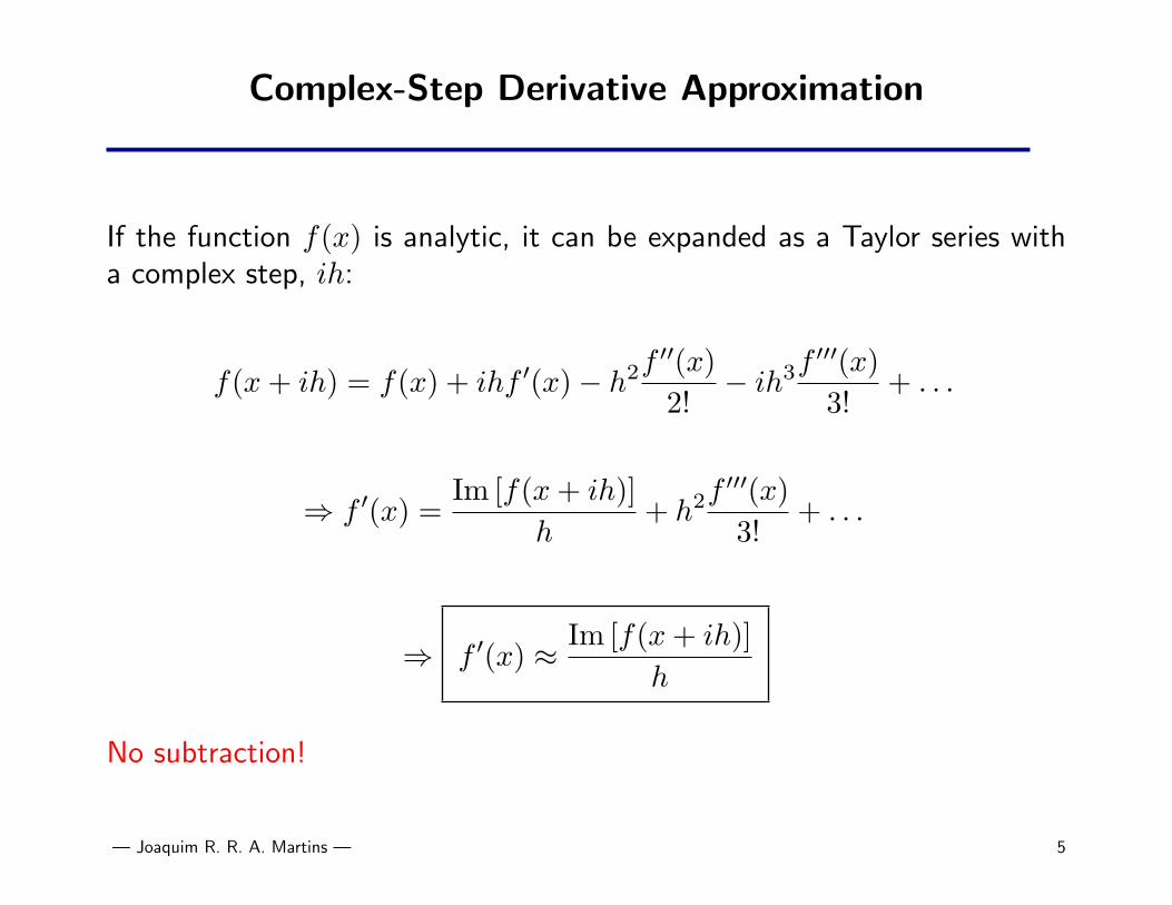
Complex-Step Derivative Approximation

If the function f(x) is analytic, it can be expanded as a Taylor series witha complex step, ih:

f(x + ih) = f(x) + ihf ′(x)− h2f′′(x)2!

− ih3f′′′(x)3!

+ . . .

⇒ f ′(x) =Im [f(x + ih)]

h+ h2f

′′′(x)3!

+ . . .

⇒ f ′(x) ≈ Im [f(x + ih)]h

No subtraction!


Why Improve the Complex-Step Method?

• Improvements necessary because,

arcsin(z) = −i log[iz +

√1− z2

],

may yield a zero derivative...

• How? If z = x + ih, where x = O(1) and h = O(10−20) then in theaddition,

iz + z = (x− h) + i (x + h)

h vanishes when using finite precision arithmetic.

• Would like to keep the real and imaginary parts separate.


Alternative Definition for “sin”

• Complex definition of sine also problematic,

sin(z) =eiz − e−iz

2i.

• Complex trigonometric relation gives better alternative:

sin(x + ih) = sin(x) cosh(h) + i cos(x) sinh(h).

• Note that for small h this simplifies to,

sin(x + ih) ≈ sin(x) + ih cos(x).


Alternative Definition for “arcsin”

• From the standard complex definition,

arcsin(z) = −i log[iz +

√1− z2

].

• Need real and imaginary parts calculated separately.

• Linearize in h about h = 0,

arcsin(x + ih) ≡ arcsin(x) + ih√

1− x2.


The Connection

• The new function definitions in these examples can be generalized:

f(x + ih) ≡ f(x) + ih∂f(x)

∂x.

• The real part is the real function and the imaginary part is the derivativemultiplied by h.

• Defining functions this way, the complex-step method is the same asalgorithmic differentiation.

• For small enough step, using finite precision arithmetic, the complex-stepmethod is the same as algorithmic differentiation.


Algorithmic Differentiation vs. Complex Step

Look at a simple operation, e.g. f = x1x2,

Algorithmic Complex-Step∆x1 = 1 h1 = 10−20

∆x2 = 0 h2 = 0f = x1x2 f = (x1 + ih1)(x2 + ih2)∆f = x1∆x2 + x2∆x1 f = x1x2−h1h2 + i(x1h2 + x2h1)df/dx1 = ∆f df/dx1 = Im f/h

Complex-step method computes one extra term.

• Other functions are similar:

– Superfluous calculations are made.– For h ≤ x× 10−20 they vanish but still affect speed.


Previously Unresolved Issues

Large body of research on algorithmic differentiation can now be applied tothe complex-step method:

• Singularities: non-analytic points

• if statements: piecewise function definitions

• Convergence for iterative solvers

• Other issues addressed by the algorithmic differentiation community


Automatic Differentiation Implementations

• Algorithmic Differentiation

– Source transformation (ADIFOR, ADIC):resulting code is unmaintainable.

– Derived datatype and operator overloading (ADOL-F, ADOL-C):far fewer changes are necessary in source code, requires object-orientedlanguage.

• Complex Step:

– Even fewer changes are required.– Resulting code is maintainable.– Can be easily implemented in any programming language that supports

complex arithmetic.


Fortran Implementation

• complexify.f90: a module that defines additional functions andoperators for complex arguments.

• Complexify.py: Python script that makes necessary changes to sourcecode, e.g., type declarations.

• New improvements:

– Script is more versatile:∗ Compatible with many more platforms and compilers.∗ Supports MPI based parallel implementations.∗ Resolves some of the input and output issues.

– Some of the function definitions were improved: tangent, inverse andhyperbolic trigonometric functions.


C/C++ Implementations

• complexify.h: defines additional functions and operators for thecomplex-step method.

• derivify.h: simple algorithmic differentiation. Defines a new typewhich contains the value and its derivative.

• Compared run time with real-valued code:

– Complexified version: ≈ ×3– Algorithmic differentiation version: ≈ ×2


2D Flow Solver: FLO82

RAE 2822 Airfoilα = 3.0o, M∞ = 0.70

1.

20

0.80

0.

40

0.00

-0.

40 -

0.80

-1.

20 -

1.60

-2.

00

Cp

+++++++++++++++++++++++++

++

+++++++++++++++++++++++++++++++++++++++++++

+

+

+

+

+

+

+

+

+

+

+

++++++++++++++++++++++++++++++++++++++++++++++++++

+

++

+++++++++++++++++++++++++++


Convergence of CD and ∂CD/∂M∞

50 100 150 200 250 300 350 400 450 500

10−15

10−10

10−5

100

Iterations

Rel

ativ

e E

rror

, εC

D

∂ CD

/ ∂ M∞

Imaginary part converges at similar rate but lagged.


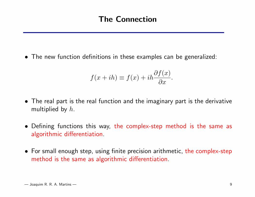
Sensitivity Estimate vs. Step Size

10−30

10−20

10−10

10−15

10−10

10−5

100

Rel

ativ

e E

rror

, ε

Step Size, h

Complex−Step Finite−difference

Complex-step is accurate from h = 10−10 to h = 10−321.


3D Aero-Structural Design Optimization Framework

• Aerodynamics: SYN107-MB, a parallel,multiblock Euler flow solver.

• Structures: detailed finite element modelwith plates and trusses.

• Coupling: high-fidelity, consistent andconservative.

• Geometry: centralized database forexchanges (jig shape, pressuredistributions, displacements.)

• Coupled-adjoint sensitivity analysis


Aero-Structural Model and Solution


Wing Structural Model Detail


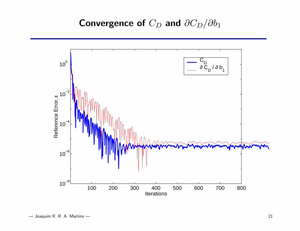
Convergence of CD and ∂CD/∂b1

100 200 300 400 500 600 700 80010

−8

10−6

10−4

10−2

100

Iterations

Ref

eren

ce E

rror

, εC

D

∂ CD

/ ∂ b1



10−15

10−10

10−5

10−6

10−5

10−4

10−3

10−2

10−1

100

Rel

ativ

e E

rror

, ε

Step Size, h

Complex−Step Finite−difference

Finite-difference is practically useless.


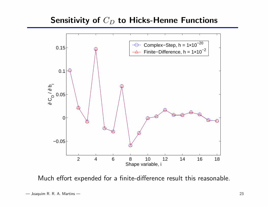
Sensitivity of CD to Hicks-Henne Functions

2 4 6 8 10 12 14 16 18

−0.05

0

0.05

0.1

0.15∂

CD

/ ∂

b i

Shape variable, i

Complex−Step, h = 1×10−20 Finite−Difference, h = 1×10−2

Much effort expended for a finite-difference result this reasonable.


Supersonic Viscous/Inviscid Solver

Tool for preliminary design of natural laminar flow supersonic aircraft

• Transition prediction

• Viscous and inviscid drag

• Design optimization– Wing planform and airfoil design– Wing-Body intersection design


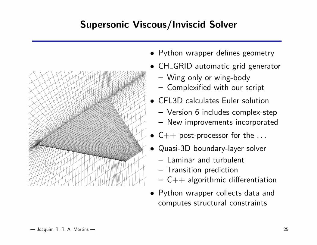
Supersonic Viscous/Inviscid Solver

• Python wrapper defines geometry

• CH GRID automatic grid generator

– Wing only or wing-body– Complexified with our script

• CFL3D calculates Euler solution

– Version 6 includes complex-step– New improvements incorporated

• C++ post-processor for the . . .

• Quasi-3D boundary-layer solver

– Laminar and turbulent– Transition prediction– C++ algorithmic differentiation

• Python wrapper collects data andcomputes structural constraints



10−20

10−15

10−10

10−5

100

10−8

10−6

10−4

10−2

100

102

Step Size, h

Rel

ativ

e E

rror

, εFinite DifferenceComplex−Step

Finite-differences truly useless.


Laminar Skin Friction CD

22.495 22.5 22.505

4.3728

4.3729

4.373

4.3731

4.3732

4.3733

4.3734

4.3735

4.3736

x 10−4

Root Chord (ft)

Cd f

Function EvaluationsComplex−Step Slope


Skin Friction CD with Transition

22.495 22.5 22.505

3.0222

3.0222

3.0222

3.0222

3.0222

3.0223

3.0223

x 10−3

Root Chord (ft)

Cd f

Function EvaluationsComplex−Step Slope


Conclusions

• Presented improvements to the complex-step method.

– Fixes to subtle problems with some complex function definitions– Simple method for defining any new function desired

• Bridged complex-step and algorithmic differentiation theories.

– Allows application of prior research to complex-step.

• Applied method to two large three-dimensional analyses.

– Automatic implementation in Fortran– Easy to implement in nearly all engineering programming languages

• Infinitely better than finite difference

– Effective in computationally noisy or poorly converged analyses– Excellent for validation of more sophisticated gradient calculations

• Tools available at: http://aero-comlab.stanford.edu/jmartins/


THE CONNECTION BETWEEN THE COMPLEX-STEP...

Documents

Transcript of THE CONNECTION BETWEEN THE COMPLEX-STEP...