The completion of Escher’s “Print Gallery”: adynamical system approach∗

P. Carphin, DMS, Universite de MontrealC. Rousseau, DMS and CRM, Universite de Montreal

October 2008

Abstract

This small note presents a visual introduction to the sequence of transformationswhich have permitted the completion of Escher’s “Print Gallery” by the team of Lenstra.The logarithm transformation and its inverse are presented as the limits of their un-foldings. These unfoldings, one of which is the Ecalle-Roussarie compensator, are wellknown functions in differential equations and dynamical systems.

1 Introduction

The present note has been motivated by the will to make visible the mathematics underlyingthe completion of Escher’s “Print Gallery” by Bart de Smit and Hendrik W. Lenstra [1].

Once Escher’s print is completed, what is obtained is a transformation from an originalprint, in which the original image is reproduced inside the image itself with a contractionfactor of C = 1

256 , to a print with infinite spiralling in itself (Figure 1). The publishing of [1]has led to the birth of a large number of programs transforming an image over the complexplane invariant under some linear contraction z 7→Cz, with |C| < 1 into an infinite spirallingimage, which we will call its “escherization”. The final image is again an image invariantunder some contraction z 7→Bz, with |B| < 1. If we restrict the original image to a rectangularframe around the center of the picture, then the image of the frame under the transformationis a spiral. Considering an image as a map F : D→ C , where C is the set of colors, thedifferent transformations are simply compositions F◦G−1, with G : D→D ′. Since conformaltransformations G are used, they can of course be written as holomorphic functions of z.The domains considered throughout the paper are either C or C∗. Indeed, when an imageis invariant under a linear contraction z 7→ Cz with |C| < 1, it is impossible to give a color tothe origin compatible with the invariance.

We use the notation LC and Pβ for the linear and power maps{LC(z) = Cz,

Pβ(z) = zβ.

∗This work is supported by NSERC in Canada.

1

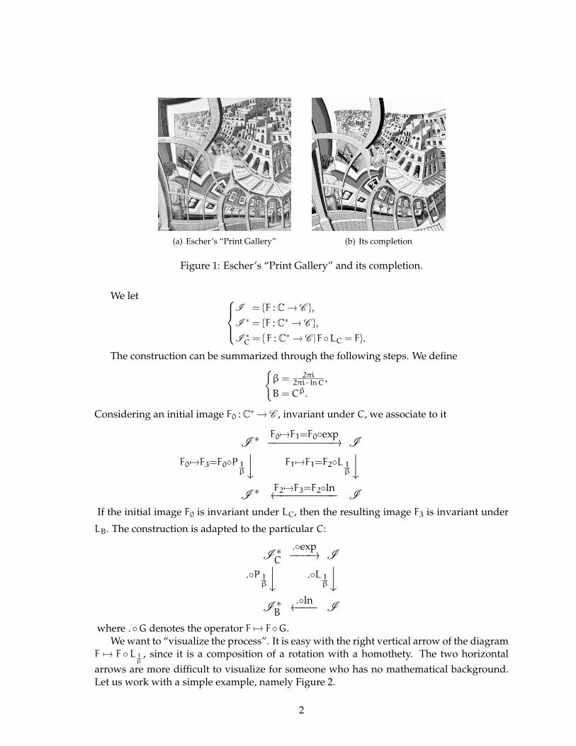
(a) Escher’s “Print Gallery” (b) Its completion

Figure 1: Escher’s “Print Gallery” and its completion.

We let I = {F : C→ C },

I ∗ = {F : C∗→ C },

I ∗C = {F : C∗→ C |F◦LC = F}.

The construction can be summarized through the following steps. We define{β = 2πi

2πi−lnC ,

B = Cβ.

Considering an initial image F0 : C∗→ C , invariant under C, we associate to it

I ∗ F0 7→F1=F0◦exp−−−−−−−−−→ I

F0 7→F3=F0◦P 1β

y F1 7→F1=F2◦L 1β

yI ∗ F2 7→F3=F2◦ln←−−−−−−−− I

If the initial image F0 is invariant under LC, then the resulting image F3 is invariant under

LB. The construction is adapted to the particular C:

I ∗C

.◦exp−−−→ I

.◦P 1β

y .◦L 1β

yI ∗

B

.◦ln←−− I

where .◦G denotes the operator F 7→ F◦G.We want to “visualize the process”. It is easy with the right vertical arrow of the diagram

F 7→ F ◦ L 1β

, since it is a composition of a rotation with a homothety. The two horizontalarrows are more difficult to visualize for someone who has no mathematical background.Let us work with a simple example, namely Figure 2.

2

Figure 2: The initial image.

Figure 3: The initial image in 3-dimensional space.

1. Upper arrow. It transforms an image invariant under LC, i.e. with a multiplicativeperiod, into an image with two additive periods. In order to understand how thishappens, we will introduce a film between the two images. We imagine ourselvesin 3-dimensional space with the image F0 on the horizontal plane (Figure 3), whichwe can think of as a table cloth. We lift the (elastic) table cloth by its center, thustransforming it into a cone (Figure 4).

(Figure 7). During the whole process we keep the unit circle fixed in the horizontalplane. Lifting up the vertex of the cone to infinity, we transform the punctured planeinto a cylinder. On the cones we still have invariance under a multiplicative periodbut, when the cone tends to the cylinder, this multiplicative period tends to 1. In thelimit when the vertex of the cone is at infinity we get a translation by a first (vertical)period T1. The process yields a uniform image on the cylinder. So, when we unroll thecylinder, we get a second independent period T2 of norm 2π.

2. Right vertical arrow. We cut the cylinder along a vertical line and slide it along thisline by one vertical period. We also scale it so that its horizontal section remains ofconstant length.

3. Lower arrow. We inverse the process of the upper arrow. The final image appears inFigure 6.

Now, how to put this visualization in equation? We want to use conformal transforma-tions all the way. The natural conformal transformation of a plane to a cone is z 7→ zα, andif the cone is to become infinitely thin, then α must decrease from 1 to 0. Simultaneously,

3

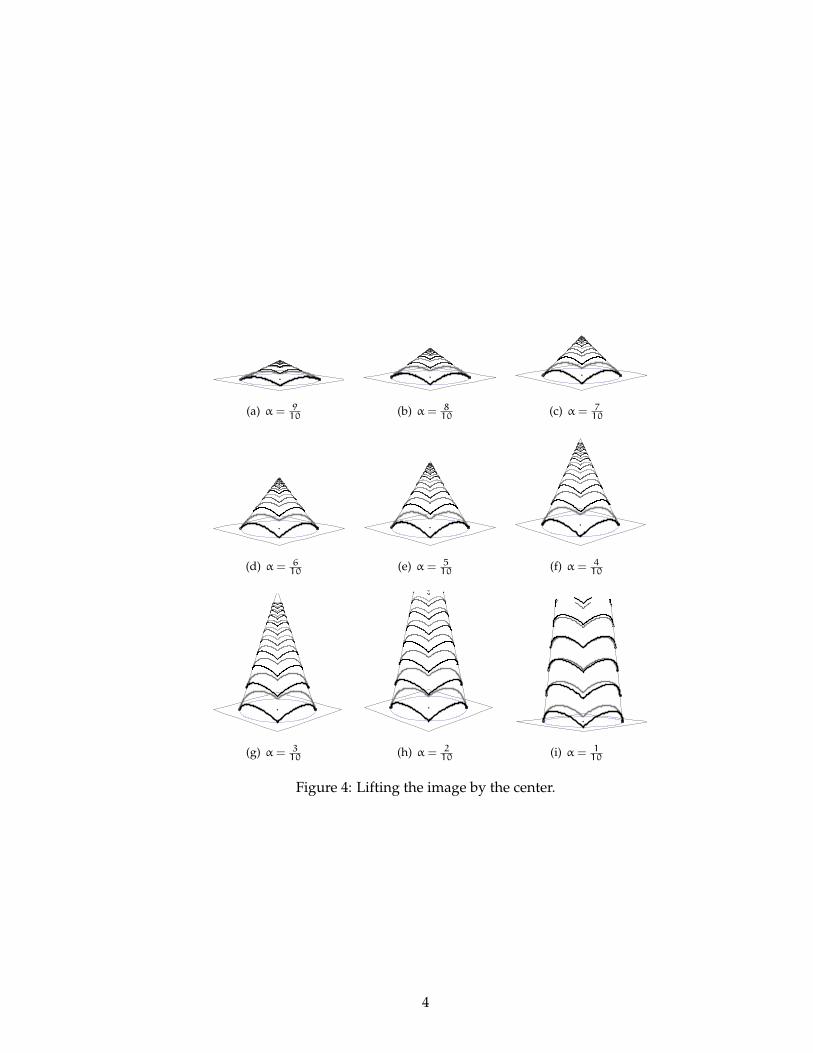
(a) α = 910 (b) α = 8

10 (c) α = 710

(d) α = 610 (e) α = 5

10 (f) α = 410

(g) α = 310 (h) α = 2

10 (i) α = 110

Figure 4: Lifting the image by the center.

4

(a) α = 110 (b) α = 2

10 (c) α = 310

(d) α = 410 (e) α = 5

10 (f) α = 610

(g) α = 710 (h) α = 8

10 (i) α = 910

Figure 5: Back from the cylinder to the plane.

Figure 6: The “escherized” final image.

5

we must send the origin to∞ and rescale, so that what we see at finite distance, the imageof the circle of radius 1, remains a curve of length 1. A way to do that is to use the functionz 7→ zα−1

α with α decreasing from 1 to 0. This just one part of the Ecalle-Leontovich-Roussariecompensator

ω(z,α) =

{zα−1

α , α 6= 0,

lnz, α = 0,

which is analytic except at z = 0. This function is well known in dynamical systems as

(a) α = 1 (b) α = 78 (c) α = 6

8

(d) α = 58 (e) α = 1

2 (f) α = 38

(g) α = 14 (h) α = 1

8 (i) α = 0.0001

Figure 7: Deformation to the logarithm function.

the natural unfolding of the logarithm function. It is not unlikely that it be known under

6

different names in other fields of mathematics. The construction of the escherization of F0

can now be visualized in the Figures 7 and 8. Note that angles are preserved throughout theprocess.

(a) (b) (c)

(d) (e) (f)

(g) (h) (i)

Figure 8: Coming back from the logarithm function.

7

References

[1] B. de Smit and H.W. Lenstra, Artful mathematics: the heritage of M. C. Escher, No-tices of the AMS 50, no 4 (2003), 446-451.

8