The Clustergram: A graph for visualizing hierarchical and non ... · 1 The Stata Journal, 2002, 3,...
19
1 The Stata Journal, 2002, 3, pp 316-327 The Clustergram: A graph for visualizing hierarchical and non-hierarchical cluster analyses Matthias Schonlau RAND Abstract In hierarchical cluster analysis dendrogram graphs are used to visualize how clusters are formed. I propose an alternative graph named “clustergram” to examine how cluster members are assigned to clusters as the number of clusters increases. This graph is useful in exploratory analysis for non-hierarchical clustering algorithms like k-means and for hierarchical cluster algorithms when the number of observations is large enough to make dendrograms impractical. I present the Stata code and give two examples. Key Words Dendrogram, tree, clustering, non-hierarchical, large data, asbestos 1. Introduction The Academic Press Dictionary of Science and Technology defines a dendrogram as follows: dendrogram Biology. a branching diagram used to show relationships between members of a group; a family tree with the oldest common ancestor at the base, and branches for various divisions of lineage.
Transcript of The Clustergram: A graph for visualizing hierarchical and non ... · 1 The Stata Journal, 2002, 3,...
1
The Stata Journal, 2002, 3, pp 316-327 The Clustergram: A graph for visualizing hierarchical and non-hierarchical cluster analyses
Matthias Schonlau
RAND
Abstract
In hierarchical cluster analysis dendrogram graphs are used to visualize how clusters are
formed. I propose an alternative graph named “clustergram” to examine how cluster
members are assigned to clusters as the number of clusters increases. This graph is useful
in exploratory analysis for non-hierarchical clustering algorithms like k-means and for
hierarchical cluster algorithms when the number of observations is large enough to make
dendrograms impractical. I present the Stata code and give two examples.
Key Words
Dendrogram, tree, clustering, non-hierarchical, large data, asbestos
1. Introduction
The Academic Press Dictionary of Science and Technology defines a dendrogram as
follows:
dendrogram Biology. a branching diagram used to show relationships between members
of a group; a family tree with the oldest common ancestor at the base, and branches for
various divisions of lineage.
2
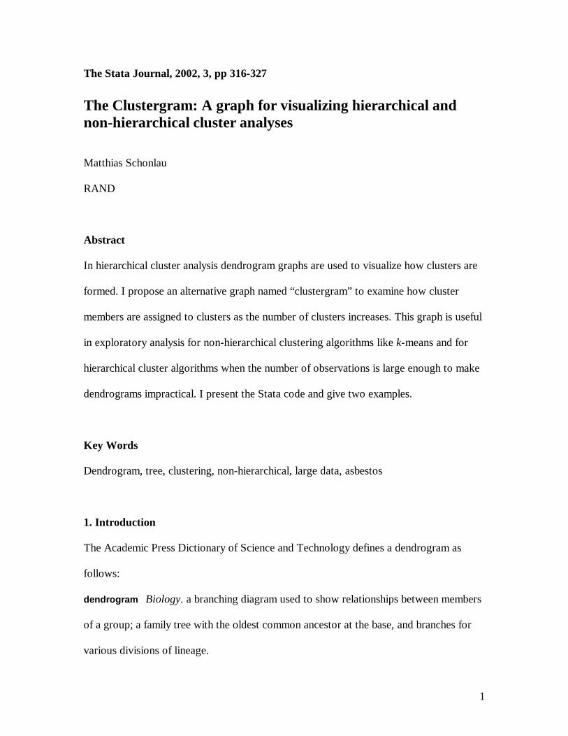
In cluster analysis a dendrogram ([R] cluster dendrogram and, for example, Everitt and
Dunn, 1991, Johnson and Wichern, 1988) is a tree graph that can be used to examine
how clusters are formed in hierarchical cluster analysis ([R] cluster singlelinkage, [R]
cluster completelinkage, [R] cluster averagelinkage). Figure 1 gives an example of a
dendrogram with 75 observations. Each leaf represents an individual observation. The
leaves are spaced evenly along the horizontal axis. The vertical axis indicates a distance
or dissimilarity measure. The height of a node represents the distance of the two clusters
that the node joins. The graph is used to visualize how clusters are formed. For example,
if the maximal distance on the y axis is set to 40, then three clusters are formed because
y=40 intersects the tree three times.
L2
diss
imila
rity
mea
sure
0
10
20
30
40
50
60
70
110322514618481271592016212241119232513172632414348422770536460716237575528463044334534364035384729493150396751746959616675525663587254736568
Figure 1 A dendrogram for 75 observations
3
Dendrograms have two limitations: (1) because each observation must be displayed as a
leaf they can only be used for a small number of observations. Stata 7 allows up to 100
observations. As Figure 1 shows, even with 75 observations it is difficult to distinguish
individual leaves. (2) The vertical axis represents the level of the criterion at which any
two clusters can be joined. Successive joining of clusters implies a hierarchical structure,
meaning that dendrograms are only suitable for hierarchical cluster analysis.
For large numbers of observations hierarchical cluster algorithms can be too time-
consuming. The computational complexity of the three popular linkage methods is of
order O(n2), whereas the most popular non-hierarchical cluster algorithm, k-means ([R]
cluster kmeans, MacQueen, 1967), is only of the order O(kn) where k is the number of
clusters and n the number of observations (Hand et al., 2001). Therefore k-means, a non-
hierarchical method, is emerging as a popular choice in the data mining community.
I propose a graph that examines how cluster members are assigned to clusters as the
number of clusters changes. In this way it is similar to the dendrogram. Unlike the
dendrogram this graph can be used for non-hierarchical clustering algorithms also. I call
this graph a clustergram.
The outline of the remainder of this paper is as follows: Section 2 and 3 contain syntax
and options of the Stata command clustergram, respectively. Section 4 explains how the
clustergram is computed by means of an example related to asbestos lawsuits. The
4
example also illustrates the use of the clustergram command. Section 5 contains a second
example: Fisher’s famous Iris data. Section 6 concludes with some discussion.
2. Syntax
clustergram varlist [if exp] [in range] , CLuster(clustervarlist)
[ FRaction(#) fill graph_options ]
The variables specifying the cluster assignments must be supplied. I illustrate this in an
example below.
3. Options
clustervarlist specifies the variables containing cluster assignments, as
previously produced by cluster. More precisely, they usually
successively specify assignments to 1, 2, ... clusters.
Typically they will be named something like cluster1 -clustermax,
where max is the maximum number of clusters identified. It is
possible to specify assignments other than to 1,2, ... clusters
(e.g. omitting the first few clusters, or in reverse order). A
warning will be displayed in this case. This option is required.
fraction()specifies a fudge factor controlling the width of line
segments and is typically modified to reduce visual clutter. The
relative width of any two line segments is not affected. The
value should be between 0 and 1. The default is 0.2.
5
fill specifies that individual graph segments are to be filled (solid).
By default only the outline of each segment is drawn.
graph_options are options of graph, twowa y other than symbol() and
connect(). The defaults include ylabels showing three (rounded)
levels and gap(5).
4. Description and the Asbestos Example
A huge number of lawsuits concerning asbestos-related personal injuries have been filed
in the United States. One interesting question is: can companies be clustered into groups
on the basis of how many lawsuits were filed against them? The data consist of the
number of asbestos suits filed against 178 companies in the United States from 1970
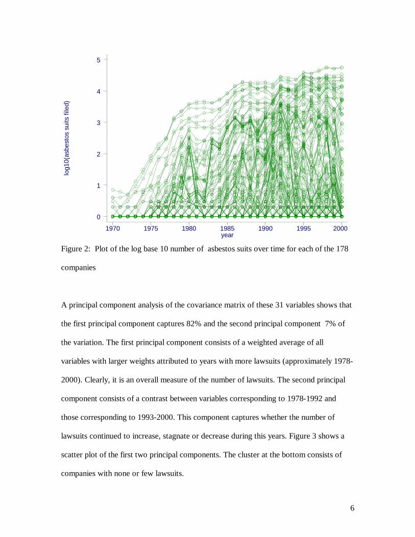
through 2000. Figure 2 shows a plot of the log base 10 of the number of asbestos suits
over time for each of the 178 companies. Few asbestos lawsuits were filed in the early
years. By 1990 some companies were subject to 10,000 asbestos related lawsuits in a
single year. I separate the number of asbestos suits by year to create 31 variables for the
cluster algorithm. Each variable consists of the log base 10 of the number of suits that
were filed against a company in a year.
6
log1
0(as
best
os s
uits
file
d)
year1970 1975 1980 1985 1990 1995 2000
0
1
2
3
4
5
Figure 2: Plot of the log base 10 number of asbestos suits over time for each of the 178
companies
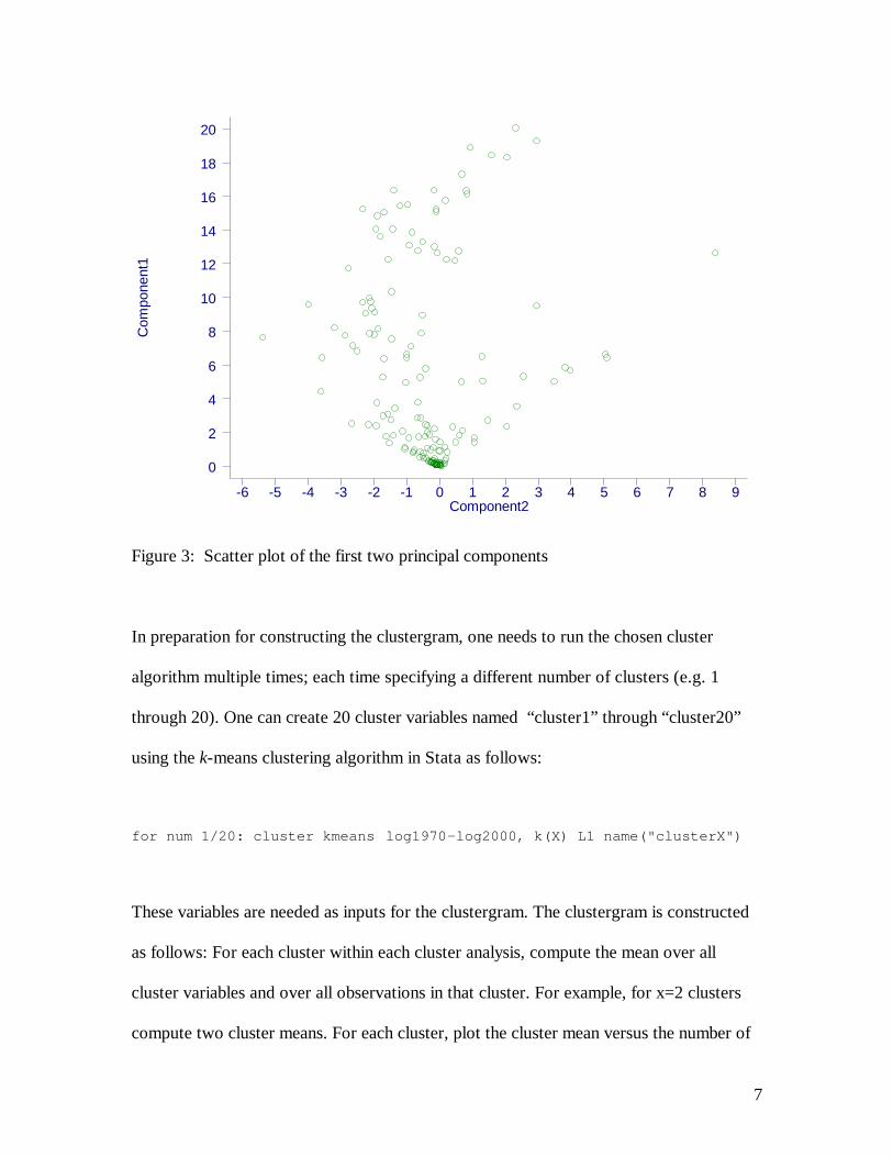
A principal component analysis of the covariance matrix of these 31 variables shows that
the first principal component captures 82% and the second principal component 7% of
the variation. The first principal component consists of a weighted average of all
variables with larger weights attributed to years with more lawsuits (approximately 1978-
2000). Clearly, it is an overall measure of the number of lawsuits. The second principal
component consists of a contrast between variables corresponding to 1978-1992 and
those corresponding to 1993-2000. This component captures whether the number of
lawsuits continued to increase, stagnate or decrease during this years. Figure 3 shows a
scatter plot of the first two principal components. The cluster at the bottom consists of
companies with none or few lawsuits.
7
Com
pone
nt1
Component2-6 -5 -4 -3 -2 -1 0 1 2 3 4 5 6 7 8 9
0
2
4
6
8
10
12
14
16
18
20
Figure 3: Scatter plot of the first two principal components
In preparation for constructing the clustergram, one needs to run the chosen cluster
algorithm multiple times; each time specifying a different number of clusters (e.g. 1
through 20). One can create 20 cluster variables named “cluster1” through “cluster20”
using the k-means clustering algorithm in Stata as follows:
for num 1/20: cluster kmeans log1970-log2000, k(X) L1 name("clusterX")
These variables are needed as inputs for the clustergram. The clustergram is constructed
as follows: For each cluster within each cluster analysis, compute the mean over all
cluster variables and over all observations in that cluster. For example, for x=2 clusters
compute two cluster means. For each cluster, plot the cluster mean versus the number of
8
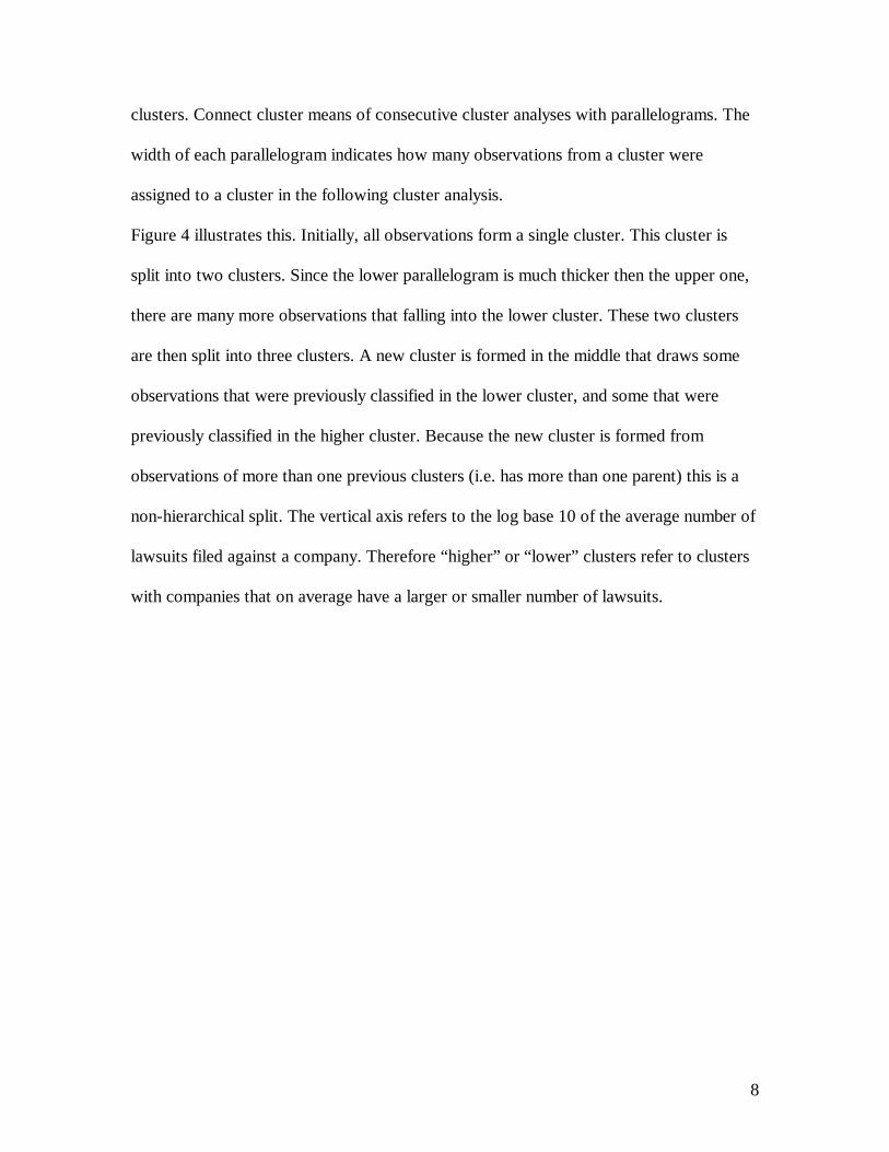
clusters. Connect cluster means of consecutive cluster analyses with parallelograms. The
width of each parallelogram indicates how many observations from a cluster were
assigned to a cluster in the following cluster analysis.
Figure 4 illustrates this. Initially, all observations form a single cluster. This cluster is
split into two clusters. Since the lower parallelogram is much thicker then the upper one,
there are many more observations that falling into the lower cluster. These two clusters
are then split into three clusters. A new cluster is formed in the middle that draws some
observations that were previously classified in the lower cluster, and some that were
previously classified in the higher cluster. Because the new cluster is formed from
observations of more than one previous clusters (i.e. has more than one parent) this is a
non-hierarchical split. The vertical axis refers to the log base 10 of the average number of
lawsuits filed against a company. Therefore “higher” or “lower” clusters refer to clusters
with companies that on average have a larger or smaller number of lawsuits.
9
Clu
ster
mea
n
Number of clusters1 2 3
0
.5
1
1.5
2
2.5
Figure 4: A clustergram for 1–3 clusters. The cluster assignments stem from the k-means algorithm.
To avoid visual clutter the width of all parallelograms or graph segments can be
controlled through a fudge factor. This factor by default is 0.2 and can optionally be set
by the user. The amount should be chosen large enough that clusters of various sizes can
be distinguished and small enough that there is not too much visual clutter.
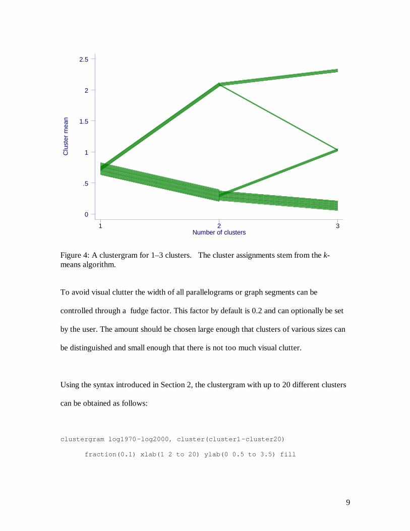
Using the syntax introduced in Section 2, the clustergram with up to 20 different clusters
can be obtained as follows:
clustergram log1970-log2000, cluster(cluster1-cluster20)
fraction(0.1) xlab(1 2 to 20) ylab(0 0.5 to 3.5) fill
10
C
lust
er m
ean
Number of clusters1 2 3 4 5 6 7 8 9 10 11 12 13 14 15 16 17 18 19 20
0
.5
1
1.5
2
2.5
3
3.5
Figure 5: Clustergram with up to 20 clusters. The k-means cluster algorithm was used.
Figure 5 displays the resulting clustergram for up to 20 clusters. We see that the
companies initially split into two clusters of unequal size. The cluster with the lowest
mean remains the largest cluster by far for all cluster sizes. One can also identify
hierarchical splits. A split is a hierarchical split when a cluster has only one parent or
predecessor. The split from 3 to 4 clusters is almost hierarchical (it is not strictly
hierarchical because a single company joins from the bottom cluster). Also, there are a
number of individual companies that appear to be hard to classify because they switch
clusters.
11
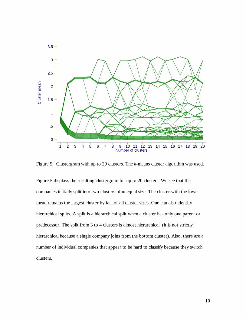
At 8 and 19 clusters the two clusters at the top merge and then de-merge again. This
highlights a weakness of the k-means algorithm. For some starting values the algorithm
may not find the best solution. The clustergram in this case is able to identify the
instability for this data set.
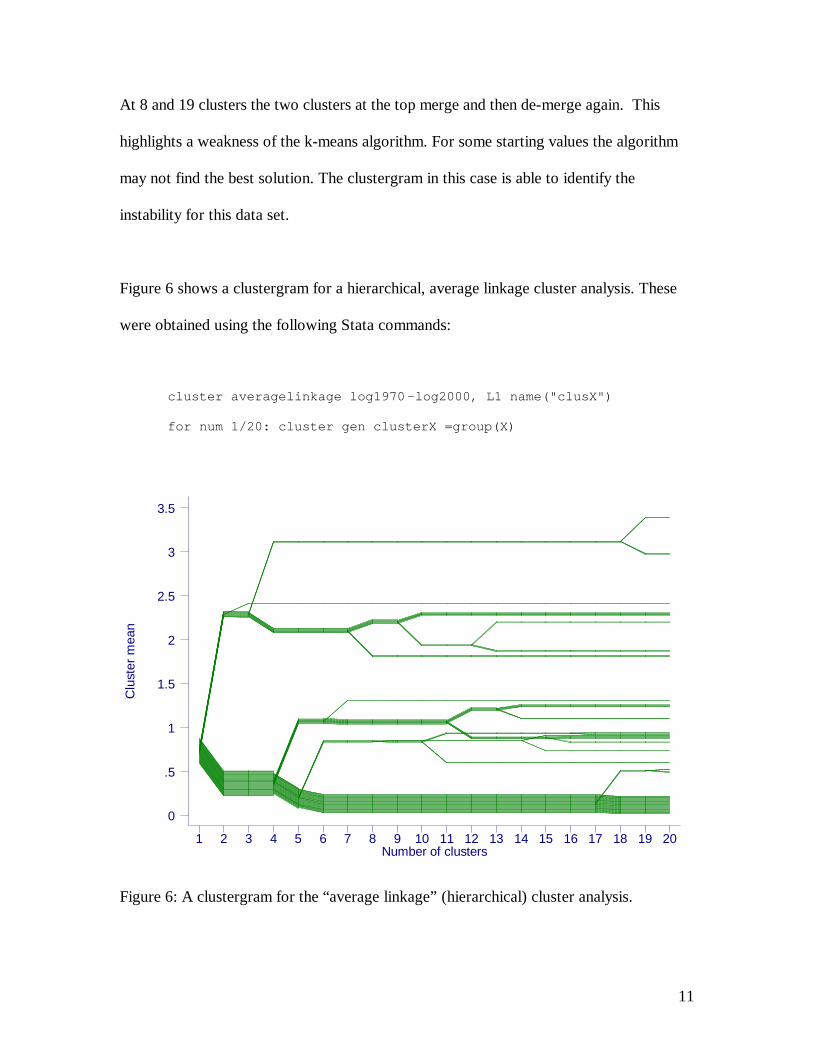
Figure 6 shows a clustergram for a hierarchical, average linkage cluster analysis. These
were obtained using the following Stata commands:
cluster averagelinkage log1970-log2000, L1 name("clusX")
for num 1/20: cluster gen clusterX =group(X)
Clu
ster
mea
n
Number of clusters1 2 3 4 5 6 7 8 9 10 11 12 13 14 15 16 17 18 19 20
0
.5
1
1.5
2
2.5
3
3.5
Figure 6: A clustergram for the “average linkage” (hierarchical) cluster analysis.
12
Because of the hierarchical nature of the algorithm, once a cluster is split off it cannot
later join with other clusters later on. Qualitatively, Figure 5 and Figure 6 convey the
same picture. Again, the bottom cluster has by far the most members, and the other two
or three major streams of clusters appear at roughly the same time with a very similar
mean.
In Figure 7 we see a clustergram for a hierarchical, single linkage cluster analysis. Most
clusters are formed by splitting a single company off the largest cluster. When the 11th
cluster is formed the largest cluster shifts visibly downward. Unlike most of the previous
new clusters the 11th cluster has more than one member and its cluster mean of about 2.5
is relatively large. The re-assignment of these companies to the 11th cluster causes the
mean of the largest cluster to drop visibly. If our goal is to identify several non-trivial
clusters, this cluster algorithm does not suit this purpose. Figure 7 conveys this
information instantly.
13
Clu
ster
mea
n
Number of clusters1 2 3 4 5 6 7 8 9 10 11 12 13 14 15 16 17 18 19 20
0
.5
1
1.5
2
2.5
3
3.5
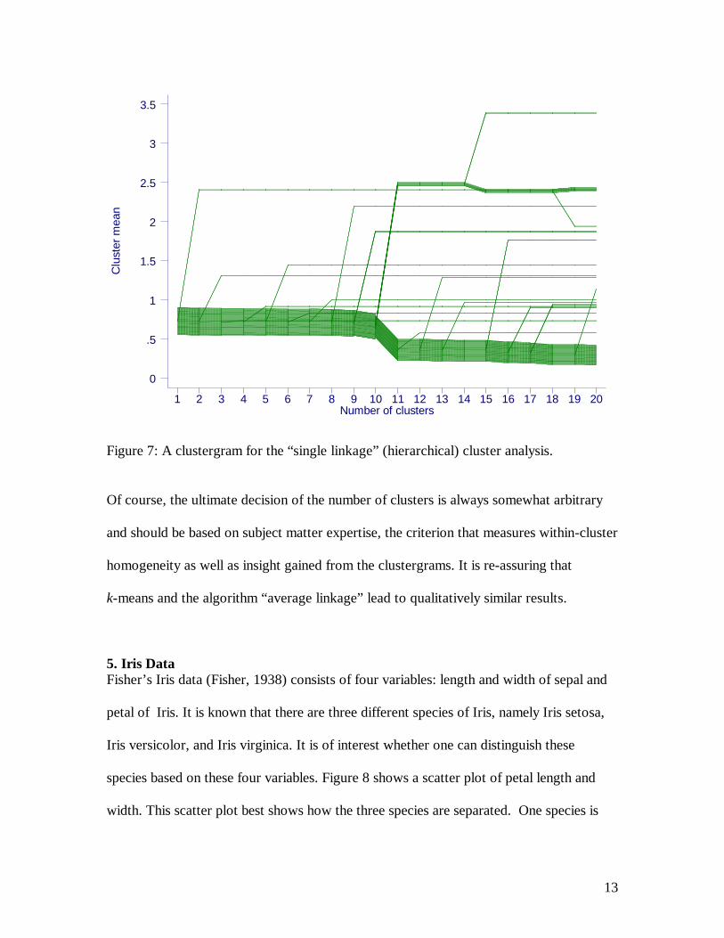
Figure 7: A clustergram for the “single linkage” (hierarchical) cluster analysis.
Of course, the ultimate decision of the number of clusters is always somewhat arbitrary
and should be based on subject matter expertise, the criterion that measures within-cluster
homogeneity as well as insight gained from the clustergrams. It is re-assuring that
k-means and the algorithm “average linkage” lead to qualitatively similar results.
5. Iris Data Fisher’s Iris data (Fisher, 1938) consists of four variables: length and width of sepal and
petal of Iris. It is known that there are three different species of Iris, namely Iris setosa,
Iris versicolor, and Iris virginica. It is of interest whether one can distinguish these
species based on these four variables. Figure 8 shows a scatter plot of petal length and
width. This scatter plot best shows how the three species are separated. One species is
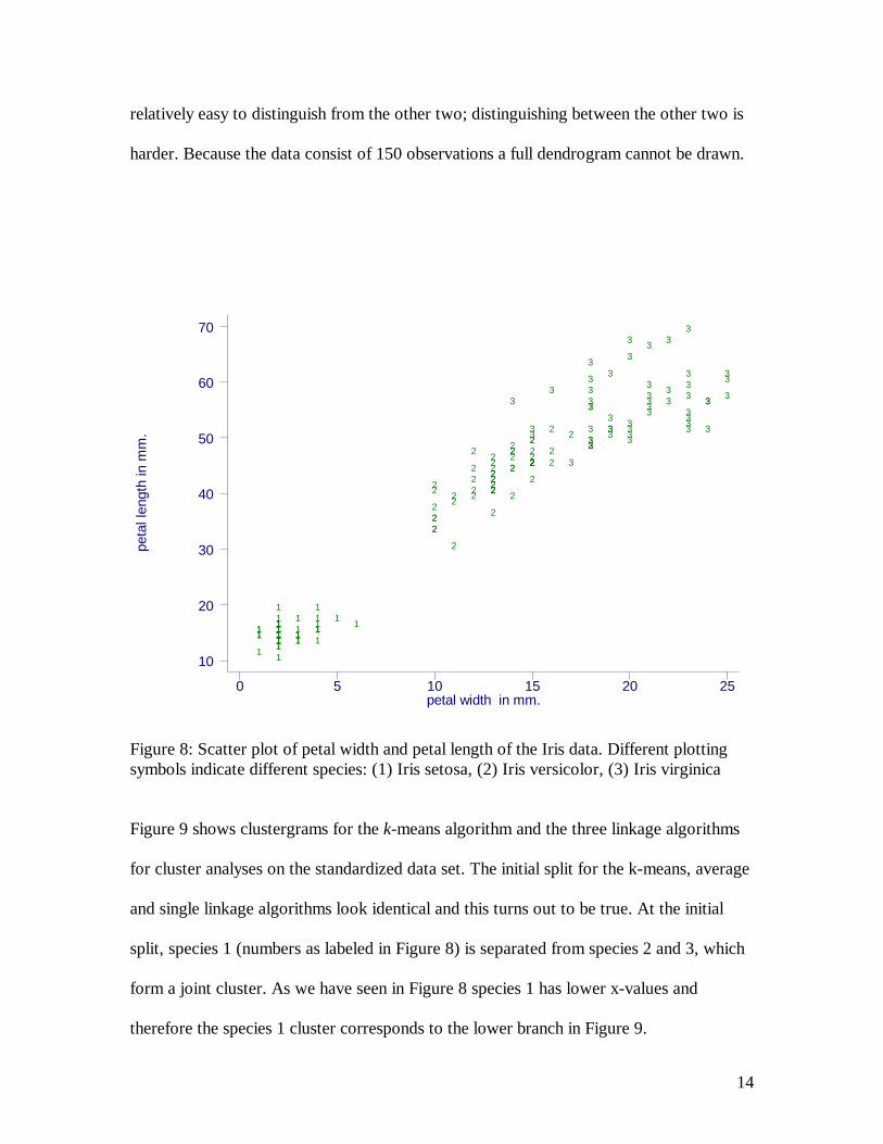
14
relatively easy to distinguish from the other two; distinguishing between the other two is
harder. Because the data consist of 150 observations a full dendrogram cannot be drawn.
peta
l len
gth
in m
m.
petal width in mm.0 5 10 15 20 25
10
20
30
40
50
60
70
1
3
2
3
3
1
3
2
2
1
2
2 3
2
3
3
3
1
2
3
3
2
3
3
3
1
3
22
2
1
3
2
3
3
11
2
3
1
3
1
2
1
3
3
1
2
2
3
11
3
1
1
1
3 3
1 1
1
2
3
11
2
2
11
2
2
11
3
3
3
2
3
11
3
3
3
3
2
22
11
3
3
1
2
2
2
11
22
2
11
3
2
3
2
11
3
2
3
3
1
2
2
1
2
22
2
2
2
3
3
11
3
3
2
2
2
33
2
11 1
3
11
2
2
2
111
32
3
1
Figure 8: Scatter plot of petal width and petal length of the Iris data. Different plotting symbols indicate different species: (1) Iris setosa, (2) Iris versicolor, (3) Iris virginica
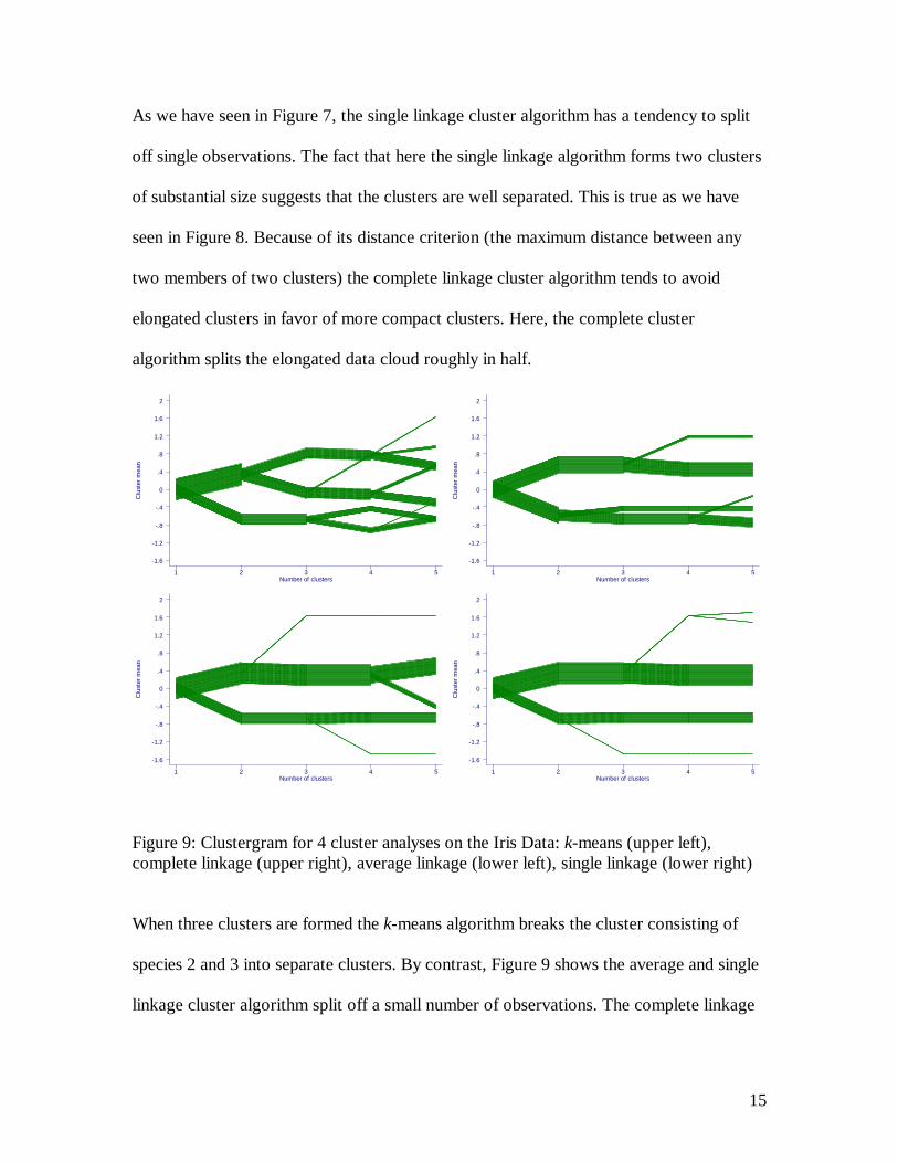
Figure 9 shows clustergrams for the k-means algorithm and the three linkage algorithms
for cluster analyses on the standardized data set. The initial split for the k-means, average
and single linkage algorithms look identical and this turns out to be true. At the initial
split, species 1 (numbers as labeled in Figure 8) is separated from species 2 and 3, which
form a joint cluster. As we have seen in Figure 8 species 1 has lower x-values and
therefore the species 1 cluster corresponds to the lower branch in Figure 9.
15
As we have seen in Figure 7, the single linkage cluster algorithm has a tendency to split
off single observations. The fact that here the single linkage algorithm forms two clusters
of substantial size suggests that the clusters are well separated. This is true as we have
seen in Figure 8. Because of its distance criterion (the maximum distance between any
two members of two clusters) the complete linkage cluster algorithm tends to avoid
elongated clusters in favor of more compact clusters. Here, the complete cluster
algorithm splits the elongated data cloud roughly in half.
Clu
ster
mea
n
Number of clusters1 2 3 4 5
-1.6
-1.2
-.8
-.4
0
.4
.8
1.2
1.6
2
Clu
ster
mea
n
Number of clusters1 2 3 4 5
-1.6
-1.2
-.8
-.4
0
.4
.8
1.2
1.6
2
Clu
ster
mea
n
Number of clusters1 2 3 4 5
-1.6
-1.2
-.8
-.4
0
.4
.8
1.2
1.6
2
Clu
ster
mea
n
Number of clusters1 2 3 4 5
-1.6
-1.2
-.8
-.4
0
.4
.8
1.2
1.6
2
Figure 9: Clustergram for 4 cluster analyses on the Iris Data: k-means (upper left), complete linkage (upper right), average linkage (lower left), single linkage (lower right)
When three clusters are formed the k-means algorithm breaks the cluster consisting of
species 2 and 3 into separate clusters. By contrast, Figure 9 shows the average and single
linkage cluster algorithm split off a small number of observations. The complete linkage
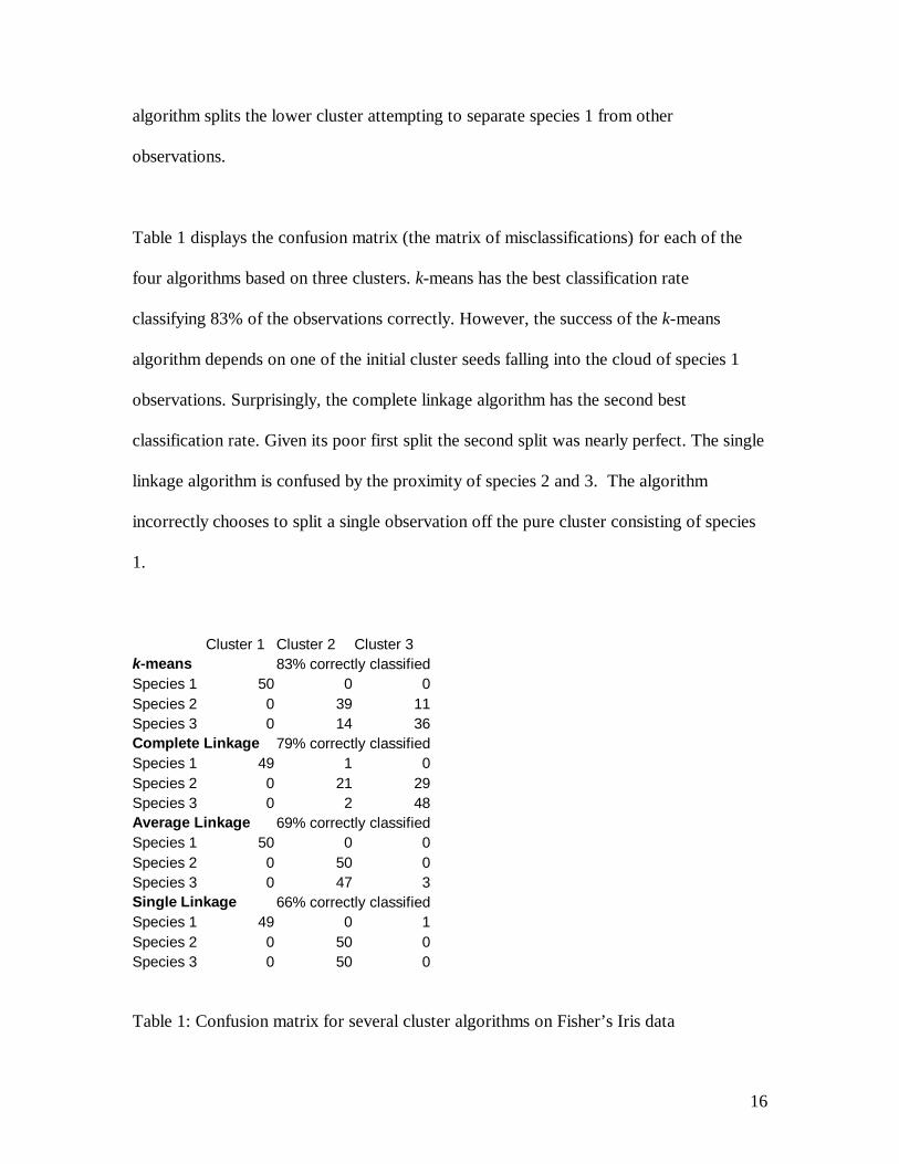
16
algorithm splits the lower cluster attempting to separate species 1 from other
observations.
Table 1 displays the confusion matrix (the matrix of misclassifications) for each of the
four algorithms based on three clusters. k-means has the best classification rate
classifying 83% of the observations correctly. However, the success of the k-means
algorithm depends on one of the initial cluster seeds falling into the cloud of species 1
observations. Surprisingly, the complete linkage algorithm has the second best
classification rate. Given its poor first split the second split was nearly perfect. The single
linkage algorithm is confused by the proximity of species 2 and 3. The algorithm
incorrectly chooses to split a single observation off the pure cluster consisting of species
1.
Cluster 1 Cluster 2 Cluster 3 k-means 83% correctly classified Species 1 50 0 0 Species 2 0 39 11 Species 3 0 14 36 Complete Linkage 79% correctly classified Species 1 49 1 0 Species 2 0 21 29 Species 3 0 2 48 Average Linkage 69% correctly classified Species 1 50 0 0 Species 2 0 50 0 Species 3 0 47 3 Single Linkage 66% correctly classified Species 1 49 0 1 Species 2 0 50 0 Species 3 0 50 0
Table 1: Confusion matrix for several cluster algorithms on Fisher’s Iris data

17
6. Discussion
The clustergram is able to highlight quickly a number of things that may be helpful in
deciding which cluster algorithm to use and / or how many clusters may be appropriate:
approximate size of clusters, including singleton clusters (clusters with only one
member); hierarchical versus non-hierarchical cluster splits; hard to classify observations;
and the stability of the cluster means as the number of clusters increase.
For cluster analysis it is generally recommended that the cluster variables be on the same
scale. Because means are computed this is also true for the clustergram. In the asbestos
claims example all variables measured the same quantity: number of lawsuits in a given
year. For most other applications – including Fisher’s Iris data - it is best to standardize
the variables.
The dendrogram is a hierarchical, binary1 tree where each branch represents a cluster.
Ultimately, at the leaves of the tree each observation becomes its own cluster. The
clustergram is a non-hierarchical tree. The number of branches varies, and can be as large
as the number of clusters. For example, observations in one of the clusters at x=10 can
branch out into any of the 11 clusters at x=11. We have only looked at up to 20 clusters.
If one were to continue to increase the number of clusters up to the point where the
number of clusters equals the number of observations, then at the leaves each cluster
consists of only one observation.
1 In the rare case of “ties” a node can have more than 2 children.
18
The clustergram differs from the dendrogram as follows: (1) The layout on the
dendrogram’s horizontal axis is naturally determined by the tree (except for some
freedom in whether to label a branch left or right). The layout of the non-hierarchical tree
is not obvious. We chose to use the mean to determine the coordinate. Other functions are
possible. (1) In the dendrogram “distance” is used as the second axis. “Distance”
naturally determines the number of clusters. In the clustergram we use the number of
clusters instead. (3) In a clustergram the (non-hierarchical) tree is not usually extended
until each leaf contains only one observation. (4) In the clustergram the width of the
parallelogram indicates cluster size. This is not necessary for the dendrogram. Since all
leaves are plotted uniformly across the horizontal axis the width of the cluster already
gives a visual cue as to its size.
The clustergram can be used for hierarchical clusters. If the data set is small enough to
display a full dendrogram a dendrogram is preferable because “distance” conveys more
information than “number of clusters”.
7. Acknowledgement
I am grateful for support from the RAND Institute of Civil Justice and the RAND
statistics group. I am grateful to Steve Carroll for involving me in the Asbestos project.
8. References
Everitt, B.S. and G. Dunn. 1991. Applied Multivariate Data Analysis, John Wiley &
Sons, New York.
19
Fisher, R.A. 1938. “The Use of Multiple Measurements in Taxonomic Problems,”
Annals of Eugenics, 8, 179-188.
Hand, D., H. Mannila and P. Smyth. 2001. Principles of Data Mining. MIT Press,
Cambridge, MA.
Johnson, R.A. and D.W. Wichern. 1988. Applied Multivariate Analysis, 2nd ed, Prentice-
Hall, Englewood Cliffs, New Jersey.
MacQueen, J. 1967. Some methods for classification and analysis of multivariate
observations. In Proceedings of the Fifth Berkeley Symposium on Mathematical
Statistics and Probability. L.M. LeCam and J. Neyman (eds.) Berkeley:
University of California Press, 1, pp. 281-297.
About the Author
Matthias Schonlau is an associate statistician with the RAND corporation and also heads
the RAND statistical consulting service. His interests include visualization, data mining,
statistical computing and web surveys.
![Exploring and Visualizing the alma of XML Documents · { XPath Query Editor by Stylus Studio [Stu07]; Although these tools o er a (textual) hierarchical view with highlighted syntax,](https://static.fdocuments.us/doc/165x107/5f3f5b4d363eda0fe33e60b2/exploring-and-visualizing-the-alma-of-xml-documents-xpath-query-editor-by-stylus.jpg)