The classification of conformal dynamical...
41
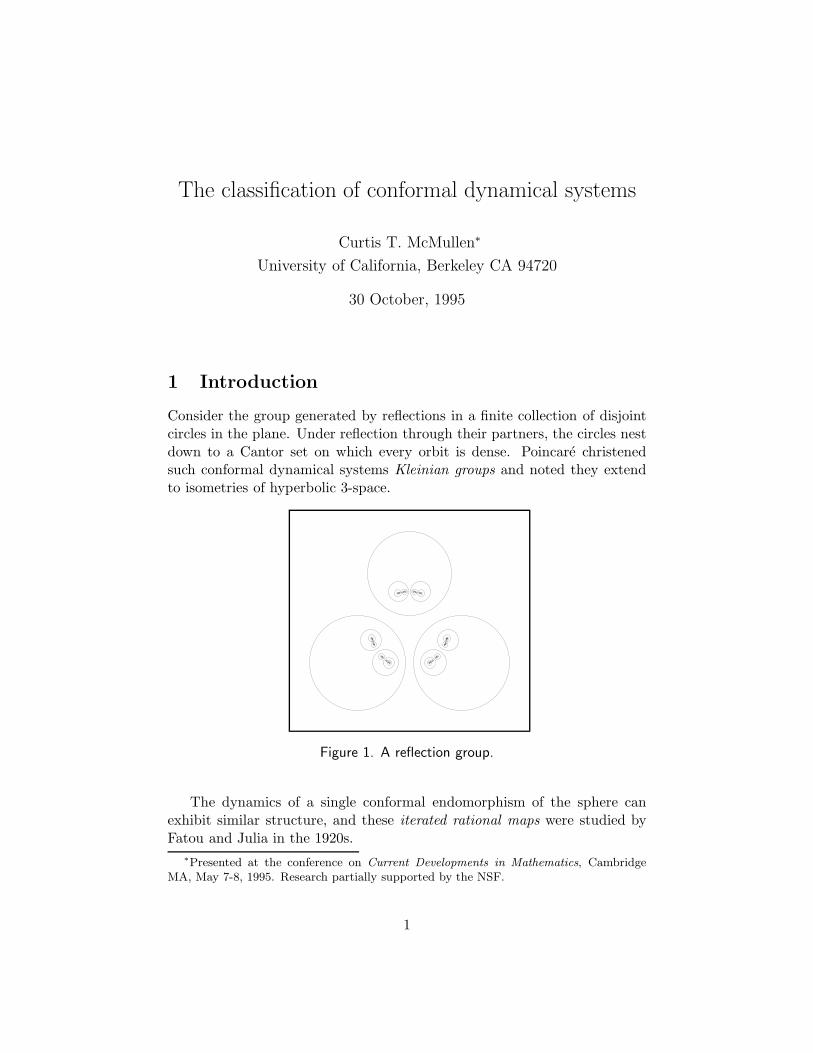
The classification of conformal dynamical systems Curtis T. McMullen ∗ University of California, Berkeley CA 94720 30 October, 1995 1 Introduction Consider the group generated by reflections in a finite collection of disjoint circles in the plane. Under reflection through their partners, the circles nest down to a Cantor set on which every orbit is dense. Poincar´ e christened such conformal dynamical systems Kleinian groups and noted they extend to isometries of hyperbolic 3-space. Figure 1. A reflection group. The dynamics of a single conformal endomorphism of the sphere can exhibit similar structure, and these iterated rational maps were studied by Fatou and Julia in the 1920s. ∗ Presented at the conference on Current Developments in Mathematics, Cambridge MA, May 7-8, 1995. Research partially supported by the NSF. 1
Transcript of The classification of conformal dynamical...
The classification of conformal dynamical systems
Curtis T. McMullen∗
University of California, Berkeley CA 94720
30 October, 1995
1 Introduction
Consider the group generated by reflections in a finite collection of disjointcircles in the plane. Under reflection through their partners, the circles nestdown to a Cantor set on which every orbit is dense. Poincare christenedsuch conformal dynamical systems Kleinian groups and noted they extendto isometries of hyperbolic 3-space.
Figure 1. A reflection group.
The dynamics of a single conformal endomorphism of the sphere canexhibit similar structure, and these iterated rational maps were studied byFatou and Julia in the 1920s.
∗Presented at the conference on Current Developments in Mathematics, CambridgeMA, May 7-8, 1995. Research partially supported by the NSF.
1

Interest in iterated rational maps was rekindled in the 1980s, whenDouady and Hubbard revealed the complexity of the family of quadraticpolynomials. Contemporaneously, Thurston’s 3-dimensional insights revolu-tionized the theory of Kleinian groups.
Sullivan discovered a dictionary between these two classical subjects.Introducing quasiconformal methods to the setting of rational maps, hetranslated Ahlfors’ finiteness theorem into a solution of the long-outstandingproblem of wandering domains.
In this paper we illustrate the dictionary by discussing the classificationproblem for conformal dynamical systems.
We begin with the Teichmuller space of a dynamical system, which classi-fies deformations and leads to the finiteness theorems of Ahlfors and Sullivan.A more detailed picture is available for expanding dynamical systems, andwe examine the conjecture that such systems are dense. Then we present theprogram for a topological classification of Kleinian groups via 3-manifolds,along with hints of a parallel theory for rational maps. The Hausdorff di-mension, ergodic theory and local connectivity of limit sets and Julia setsare also discussed. Finally we describe the role of renormalization in recentprogress on the classification of quadratic polynomials.
Notes and references are collected at the end.
2 Finiteness theorems and Teichmuller space
Definitions. A Kleinian group Γ is a discrete subgroup of the conformalautomorphism group Aut(C) of the Riemann sphere. We make the essentialassumption that Γ is finitely generated. For convenience, we also assume Γ istorsion-free, orientation-preserving, and every abelian subgroup has infiniteindex. Elements of Γ can be represented concretely as Mobius transforma-tions γ(z) = (az + b)/(cz + d).
According to the dynamics of Γ, the sphere is partitioned into the limitset Λ and the domain of discontinuity Ω. The limit set is the locus of chaoticbehavior. It is a compact, perfect set which can be defined as:
• the smallest closed Γ-invariant set with |Λ| > 2;
• the set of accumulation points of any orbit Γx ⊂ C;
• the closure of the set of repelling fixed points of γ ∈ Γ; or
2
• the set of points near which Γ does not form a normal family.1
On the other hand, Γ acts freely and conformally on Ω = C− Λ, preservingthe Poincare metric of constant curvature −1 provided by the uniformizationtheorem. Thus X = Ω/Γ is a disjoint union of hyperbolic Riemann surfaces.
A classical result in Kleinian groups is:
Theorem 2.1 (Ahlfors’ finiteness theorem) The quotient surface X isisomorphic to a finite union of compact Riemann surfaces with a finite num-ber of points removed.
In particular, every component of Ω has a nontrivial stabilizer; there isno wandering component.
Now let f : C → C be a rational map, whose iterates fn = f f . . . fare to be studied. We will assume the topological degree d of f is at leasttwo, so f(z) = P (z)/Q(z) for two relatively prime polynomials with d =max(degP,degQ) ≥ 2.
We again obtain a partition of the sphere into the Julia set J and theFatou set Ω according to the dynamics of f . The Julia set is a closed, perfectset, defined as
• the smallest closed set with f−1(J) = J and |J | > 2;
• the closure of the set of repelling periodic points of f ; or
• the set of points near which 〈fn〉 does not form a normal family.
As f is proper, it maps components of Ω to components. Perceivingthe analogy with Ahlfors’ theorem, in the early 1980s Sullivan resolved aproblem left open by Fatou and Julia in the 1920s by establishing:
Theorem 2.2 (No wandering domains) Every component of the Fatouset eventually cycles, and there are only finitely many periodic components.
One then has a fairly complete topological picture of the dynamics of f ,since a component Ω0 of the Fatou set of period p is of exactly one of thefollowing types:
1. An attractive basin: there is an x ∈ Ω0, fixed by fp, with 0 < |(fp)′(x)| <1, attracting all points of Ω0 under iteration of fp. (This is the genericcase).
1A family of maps γα : U → C is normal if every sequence has a subsequence converginguniformly on compact subsets of U .
3
2. A superattractive basin: as above, but x is a critical point of fp, so(fp)′(x) = 0.
3. A parabolic basin: there is a point x in ∂Ω0 with (fp)′(x) = 1, attract-ing all points of Ω0.
4. A Siegel disk: Ω0 is conformally isomorphic to the unit disk, and fp
acts by an irrational rotation.
5. A Herman ring: Ω0 is isomorphic to an annulus, and fp acts by anirrational rotation.
Teichmuller theory. Underlying these finiteness theorems is a descriptionof the Teichmuller space of a conformal dynamical system.
It is a remarkable fact that a measurable field of tangent ellipses ofbounded eccentricity determines a complex structure on the sphere. Thisellipse field is recorded by a (−1, 1)-form µ(z)dz/dz with ‖µ‖∞ < 1. Sincethe sphere admits a unique complex structure, there is a homeomorphismφ : C → C such that µ is the pullback of the standard structure. The con-ditions on µ imply that φ is a quasiconformal map: it has derivatives in L2,and ∂φ = µ∂φ.
The Teichmuller space Teich(Γ) classifies Kleinian groups Γ′ equippedwith quasiconformal conjugacies φ to Γ. Points in this space are determinedby Γ-invariant complex structures µ on C. The discussion is simplified bySullivan’s:
Theorem 2.3 (No invariant line fields) The limit set of a finitely gen-erated Kleinian group carries no measurable Γ-invariant field of tangentlines.
Thus any Γ-invariant µ vanishes on the limit set (otherwise the majoraxes of the corresponding ellipse field would give invariant lines). On theother hand, µ|Ω descends to a complex structure on the quotient Riemannsurface X, yielding:
Corollary 2.4 There is an isomorphism between the Teichmuller space ofΓ and that of its quotient Riemann surface X = Ω/Γ :
Teich(Γ) ∼= Teich(X).
4

Given a group G, let
V(G) = Hom(G,Aut(C))/conjugation
denote the representation variety of G, and let AH(G) ⊂ V(G) be the sub-space of discrete, faithful representations.
A conjugacy φ from Γ to Γ′ determines an isomorphism of groups, so wehave a map
δ : Teich(Γ) → AH(Γ) ⊂ V(Γ).
Since Γ is finitely generated, V(Γ) is finite-dimensional; the fibers of δ arediscrete, and therefore the Teichmuller space of X is also finite-dimensional.In other words, each component of X has finitely many moduli, so it isisomorphic to a compact Riemann surface with a finite number of pointsremoved.
This completes the proof of Ahlfors’ finiteness theorem, except for thefact that infinitely many components ofX might be triply-punctured spheres,which have no moduli; this possibility was ruled out by Greenberg.
The rigidity of the triply-punctured sphere is equivalent to the vanishingof any holomorphic quadratic differential with at worst simple poles at thepunctures. By considering differentials of higher order, one obtains:
Theorem 2.5 (Bers) If Γ is generated by N elements, then the hyperbolicarea of Ω/Γ is bounded by 4π(N − 1).
The line fields problem for rational maps. The absence of invariantline fields is equivalent to the assertion that a finitely generated Kleiniangroup is quasiconformally rigid on its limit set. In particular, if Λ = C thenΓ has a trivial Teichmuller space — it admits no deformations.
A literal translation of this result is false for rational maps, due to theLattes examples.
Let T = C/L be a complex torus, and let F : T → T be the mapF (x) = nx for n > 1. The quotient of T by the equivalence relation x ∼ −xis the Riemann sphere; the quotient map ℘ : X → C can be given by theWeierstrass ℘-function, which presents T as a twofold cover of the spherebranched over four points. Since F (−x) = −F (x), the dynamical system Fdescends to a rational map f such that the diagram
TF
−−−−→ T
℘
y ℘
y
Cf
−−−−→ C
5
commutes.Repelling periodic points for F are dense on the torus, so the Julia set of f
is the whole sphere. The map x 7→ nx preserves the family of horizontal linesin the plane, so F has an invariant line field on T (tangent to the foliationby parallel closed geodesics.) This line field descends to the Riemann sphere(with singularities at the four branch points) to give an invariant line fieldfor f .
The existence of this line field reflects the fact that, although J(f) = C,f is not rigid: it can be deformed by changing the shape of the torus T .
A fundamental problem is to show these are the only examples:
Conjecture 2.6 (No invariant line fields for rational maps) The Ju-lia set of a rational map f carries no invariant line field, except if f is aLattes example.
We will see later (Corollary 3.7) that this conjecture implies the densityof expanding dynamical systems.
The Teichmuller space of f . The space Teich(f) classifies rational mapsg equipped with quasiconformal conjugacies φ to f . It maps with discretefibers to the moduli space
Vd = Ratd /conjugation
of all rational maps of degree d, so it is finite-dimensional.To describe it, we form an analogue of the quotient surface for a Kleinian
group. Let J ⊃ J denote the closure of the grand orbits of all critical pointsand periodic points of f .2 Let Ω = C− J ; then f : Ω → Ω is a covering map,hence a local isometry for the Poincare metric. Decompose Ω as Ωdis ⊔ Ωfol
depending on whether or not the grand orbits are locally discrete.The space X = Ωdis/f is a union of Riemann surfaces; each attracting
or parabolic basin contributes a torus or cylinder with punctures to X.The space Ωfol consists of points tending to Siegel disks, Herman rings
or superattracting cycles. Each component of Ωfol is a dynamically foliatedpunctured disk or annulus.
Since we do not know if the Julia set of f carries an invariant line fieldor not, we need to include a factor M1(J, f) consisting of all f -invariant µon J with ‖µ‖ < 1. Then we have:
2Two points x, y belong to the same grand orbit if fn(x) = fm(y) for some n,m > 0.
6

Theorem 2.7 The Teichmuller space of a rational map is canonically theproduct of the finite-dimensional Teichmuller space of the quotient surfaceΩdis/f and a pair of finite polydisks:
Teich(f) ∼= Teich(Ωdis/f)× Teich(Ωfol, f)×M1(J, f).
Proof of no wandering domains. We can now complete the proof ofSullivan’s finiteness theorem. First, a wandering domain would give riseto an open disk (possibly with finitely many punctures) as a component ofΩdis/f ; since the Teichmuller space of a disk is infinite-dimensional, this is acontradiction. Each attracting basin or Herman ring contributes at least onecomplex modulus to f , so the total number of periodic regions of these twotypes is bounded. The remaining types of regions are bounded by countingcritical points and indifferent cycles.
Using quasiconformal surgery, one has the sharper estimate:
Theorem 2.8 (Shishikura) Let N be the total number of cycles of periodiccomponents in the Fatou set, H the number of cycles of Herman rings, andI the number of nonparabolic indifferent cycles in the Julia set. Then
N +H + I ≤ 2 deg(f)− 2.
Examples. Let X be a hyperbolic Riemann surface of finite area. Then Xcan be presented as the quotient of the unit disk ∆ by the action of a Fuchsiangroup Γ ⊂ Aut(∆). By Schwarz reflection Γ acts on the sphere as a Kleiniangroup, with limit set Λ = S1. Letting X denote the complex conjugate ofX, we have Ω/Γ = X ⊔X and thus Teich(Γ) = Teich(X)× Teich(X).
As one moves away from the Fuchsian locus while remaining in Teich(Γ),the limit set becomes a fractal curve of dimension strictly greater than one.3
This curve can be geometrically complicated but it remains a quasicircle:that is, it is a Jordan curve such that for any x, y ∈ Λ, the smaller subarcΛ(x, y) joining x to y satisfies
diamΛ(x, y) ≤ K|x− y|.
Finally when one reaches the boundary of Teich(Γ) in AH(Γ), some points inΛ can become identified and the topology of the limit set abruptly changes.
The case where X is a once-punctured torus is particularly easy to com-pute with, because π1(X) ∼= Z∗Z is a free group; see Figure 2. The simplest
3Poincare writes “Ces deux domaines sont separes par une ligne L, si l’on peut appelercela une ligne.”
7

Figure 2. Limit sets.
8

Figure 3. Julia sets.
9

type of point on the boundary of Teichmuller space is depicted in the finalframe: a simple curve on the torus has been pinched to a cusp, splitting Ωinto countably many components.
A proper holomorphic map or Blaschke product f : ∆ → ∆ is like aFuchsian group; by Schwarz reflection again, it extends to a rational map onthe sphere. If f has a fixed point in the disk then this point is attracting orsuperattracting and the Julia set J = S1.
Figure 4. Newton’s method for 4z3 − 2z + 1
The simplest Blaschke product is f(z) = z2. For |λ| < 1 the mapsfλ(z) = λz + z2 are all quasiconformally conformally conjugate on theirJulia sets, which are again fractal quasicircles. For 0 < |λ| < 1, these mapsbelong to a single Teichmuller space; z = 0 is an attracting fixed pointyielding a once-punctured torus as the quotient Riemann surface. Figure 3depicts Julia sets for λ approaching exp(2πi3/5); in the first three frames,|λ| < 1, while in in the final frame the attracting fixed point has becomeparabolic, splitting the Fatou set into countably many components, five ofwhich meet at the origin. The pictures are centered at the critical pointz = −λ/2.
Figure 4 depicts the dynamics of a more complicated rational map,namely Newton’s method for a cubic polynomial. This map has superat-tracting cycles at the three roots of the polynomial, and another superat-tracting cycle of period two. (Initial guesses in the basin of this last cycle donot converge to a root.) Regions in the figure are shaded to indicate which
10

of the four attractors they tend to.
3 Expanding dynamics
Crucial to the modern theory of Kleinian groups is the insight that theaction of Γ extends isometrically to hyperbolic space H3. Thus Γ determinesa Kleinian manifold
M =M ∪ ∂M = (H3 ∪ Ω)/Γ
with a complete metric of constant negative curvature on its interior and aconformal structure on its boundary.
Conversely, let M be a 3-manifold with a metric of constant curvature−1; pursuant to our standing assumptions about Γ, we will always assumeMis oriented and π1(M) is finitely generated. Then M gives rise to a Kleinian
group, by letting Γ = π1(M) acting on the compactification of M ∼= H3 bythe Riemann sphere.
Perhaps the most prominent gap in the dictionary is summed up by:
Question 3.1 Is there a 3-dimensional geometric object naturally associatedto a rational map f?
The best behaved dynamical systems have expanding properties. ForKleinian groups, expansion is reflected in the geometry of M .
To describe this relation, let hull(Λ) ⊂ H3 denote the convex hull of thelimit set, i.e. the smallest convex set containing all geodesics with bothendpoints in Λ. Let K = hull(Λ)/Γ ⊂ M be the convex core of M ; it is thesmallest convex set containing all the closed geodesics in M . We say M isgeometrically finite if a unit neighborhood of K has finite volume. A cusp ofM is a component of the thin part with parabolic fundamental group.
The following are equivalent:
• The convex core of M is compact.
• The Kleinian manifold M is compact.
• M is geometrically finite without cusps.
• For all x ∈ Λ there is a γ ∈ Γ such that ‖γ′(x)‖ > 1 with respect tothe spherical metric.
11

In this case we say Γ is expanding, or convex cocompact.The examples in Figure 2 are geometrically finite, but not expanding,
because they have cusps. Limit sets of expanding groups appear in Figures5 and 6 below.
For rational maps, the nonexpanding behavior is closely tied to the crit-ical points of f . Let
P =⋃
n>0, f ′(c)=0
fn(c)
denote the postcritical set of f , i.e. the closure of the forward orbits of thecritical points. Then the following are equivalent:
• P ∩ J = ∅.
• There are no critical points or parabolic cycles in the Julia set.
• All critical points converge to attracting or superattracting cycles un-der iteration.
• For all x ∈ J there is an n > 0 such that ‖(fn)′(x)‖ > 1.
In this case we say f is expanding.4 The Newton’s method example in Figure4 and the first three frames in Figure 3 are expanding.
Expanding dynamical systems have many robust features.
1. Openness. The space of expanding maps is open in Vd, and the spaceof expanding Kleinian groups is open in V(G).
2. Structural stability. Any dynamical system close enough to an expand-ing one is quasiconformally conjugate to it on its limit set or Julia set.
3. Finiteness. An expanding dynamical system can be described by afinite amount of data. For a Kleinian group the topology of a convexsubmanifold suffices. For a rational map one may find a pair of finitelyconnected neighborhoods U ⊂ V of the Julia set such that f : U → Vis a covering map.
4. Quasi-self-similarity. Because of expansion, any small ball meetingthe Julia set or limit set can be blown up to definite size with boundeddistortion. Thus all features of J or Λ are replicated everywhere andat all scales.
4We avoid using the more common terminology hyperbolic, to minimize confusion withhyperbolic manifolds.
12
5. Fractal geometry. Apart from the case where Λ = C, the Julia setand limit set have Hausdorff dimension δ with 0 < δ < 2, and finite,positive Hausdorff measure in this dimension. The Hausdorff measurecan be constructed dynamically as a weak limit of probability measures
limsցδ
1
Cs
∑
γ(y)=x
‖γ′(y)‖−sδy
for Kleinian groups, and
limsցδ
1
Cs
∑
fn(y)=x
‖(fn)′(y)‖−sδy
for rational maps; here x is any point with an infinite orbit outside thelimit set or Julia set. (The constants Cs normalize the total mass to1.)
If a rational map f is expanding, then there is a finite set A (the union ofthe attracting and superattracting cycles) such that fn(x) converges to thisfinite attractor for all x in the Fatou set (an open, dense full measure subsetof the sphere.) Thus we have a simple picture of the asymptotic behavior ofa typical point.
Experimentally, expanding groups and rational maps are ubiquitous. Wecan now state two central conjectures.
Conjecture 3.2 Let G be a torsion-free group which does not contain Z⊕Z.Then convex compact groups are dense in AH(G).
Conjecture 3.3 For any degree d, the expanding rational maps are densein the space of all rational maps of degree d.
The theory of holomorphic motions is a basic tool in the construction ofquasiconformal conjugacies, which leads to the following pair of tantalizingresults:
Theorem 3.4 (Mane-Sad-Sullivan) Structural stability is dense in Ratd.
Theorem 3.5 (Sullivan) A structurally stable Kleinian group is expand-ing.
13
To prove the density of convex cocompact groups, it would suffice totranslate the first result to the setting of Kleinian groups. The problem isthat for rational maps, one can work in the full moduli space of rational mapsVd, while for Kleinian groups one must restrict attention to the subspaceAH(G) of discrete faithful representations in V(G). The topology of AH(G)is not well-understood; indeed conjecture 3.2 is equivalent to the assertionthat AH(G) is the closure of its interior.
Generalizing the second result to the setting of rational maps would provethe density of expanding dynamics. Here one knows:
Theorem 3.6 There is an open dense set U ⊂ Vd such that any f, g inthe same component U0 of U are quasiconformally conjugate on the wholesphere. Thus U0 is uniformized by the Teichmuller space of f .
By counting dimensions, one can show that a structurally stable rationalmap f with no invariant line fields on its Julia set must be expanding. Thisyields:
Corollary 3.7 The no invariant line fields conjecture implies the density ofexpanding rational maps.
4 Topology of hyperbolic 3-manifolds
We now turn to the classification problem for rational maps and Kleiniangroups. Ultimately, one would like to
1. attach a combinatorial invariant to each dynamical system,
2. describe all invariants which arise, and
3. parameterize all systems with the same invariants.
The last goal is fulfilled by the Teichmuller theory discussed in §2, so it isenough to find a combinatorial invariant which determines the quasiconfor-mal conjugacy class of a rational map or Kleinian group.
This section presents the conjectural classification of Kleinian groups.The measurable and topological dynamics on the sphere are also brieflydiscussed.
3-manifolds. The classification of a Kleinian group Γ up to quasiconformalconjugacy is the same as the classification ofM = H3/Γ up to quasi-isometry.A combinatorial invariant for M can be presented in terms of 3-dimensionaltopology.
14
To begin with, suppose Γ is expanding. Then the desired combinatorialinvariant is simply the compact Kleinian manifold N = M , regarded as atopological space. It is not hard to see that the topology of N determinesthe quasi-isometry type of M . Indeed, given an end of M diffeomorphic toS × [0,∞), choose a hyperbolic metric ρ(x)dx2 on S; then the model metricetρ(x)dx2 + dt2 is quasi-isometrically correct on this end.
Now suppose M is geometrically finite. Some additional informationmust be included to specify the cusps of M . In this case the combinatorialinvariant is a pared manifold (N,P ), where N is compact and P is a sub-manifold of ∂N . The pair (N,P ) is determined by the conditions (a) M isdiffeomorphic to the interior of N and (b) M is diffeomorphic to N − P .The parabolic locus P contains every torus component of ∂N ; the rest of Pconsists of a finite number of annuli on ∂N . We then have:
Theorem 4.1 (Marden) The topology of the pared manifold (N,P ) deter-mines M up to quasi-isometry.
Finally assume only that M is an orientable hyperbolic 3-manifold withπ1(M) finitely generated. In this case the conjectural invariant is a triple(N,P, ǫ), where ǫ is the ending lamination. To even define this invariant, weneed to first assume:
Conjecture 4.2 (Tameness) A hyperbolic 3-manifold M with finitely gen-erated fundamental group is topologically tame: that is, M is diffeomorphicto the interior of a compact manifold N .
It is known that M is homotopy equivalent to a compact manifold, butexamples like the Whitehead continuum show the ends of a 3-manifold withfinitely generated fundamental group need not be products.
Assuming M is diffeomorphic to int(N), we again can locate a paraboliclocus P ⊂ N specifying the finite set of cusps. A cusp can be thoughtof as a simple curve on ∂N whose length in M has shrunk to zero. Theending lamination records a generalization of this phenomenon, in which an“irrational” simple curve has been pinched.
Given a surface S, endowed with a hyperbolic metric for convenience,a lamination λ ⊂ S is a closed subset which is a union of disjoint simplegeodesics. To construct the ending lamination, fix a diffeomorphism be-tween intN and M , so that a neighborhood of P maps into the cusps ofM . Consider any sequence of simple closed curves γn on a component S
15

of ∂N − P whose geodesic representatives in M converge to S. Then asubsequence converges, in a natural sense, to a lamination λ on S.5
The ending lamination ǫ is the union of all λ which arise this way.
Conjecture 4.3 (The ending lamination conjecture) The pared man-ifold (N,P ) and the ending lamination ǫ determine M up to quasi-isometry.
This conjecture is open even for N = S × [0, 1] where S is a compactsurface. Recently (March 1995) Minsky has announced:
Theorem 4.4 The ending lamination conjecture is true for
(N,P ) = (S × I, ∂S × I),
where S is a torus with a disk removed.
The space of laminations on a punctured torus is a circle (since a lamina-tion is determined by a line in H1(S, ∂S,R)). Bers defined a compactificationof Teichmuller space using limits of quasifuchsian groups; by Minsky’s re-sult, the compactifying points for a punctured torus are determined by theirlaminations, and we have:
Corollary 4.5 The Bers’ boundary of the Teichmuller space of a puncturedtorus is a Jordan curve.
Here are two more general results bearing on the tameness and endinglamination conjectures.
A map f : S → N of a surface into a 3-manifold is incompressible iff∗ : π1(S, p) → π1(N) is injective for all p ∈ S. A compact 3-manifold hasincompressible boundary if ∂N ⊂ N is incompressible. An open 3-manifoldM has incompressible ends if it contains an embedded compact submanifoldwith incompressible boundary, such that N →M is a homotopy equivalence.
Theorem 4.6 (Thurston, Bonahon) Any hyperbolic 3-manifold with in-compressible ends is topologically tame.
Theorem 4.7 (Minsky) Any two hyperbolic manifolds M1 and M2 withincompressible ends, injectivity radii bounded below and the same combina-torial invariant (N, ǫ) are quasi-isometric.
5The precise definition of convergence is that there is a projective measured lamination[λ0] with support λ such that [γn] → [λ0].
16

All of these results are based on a study of incompressible surfacesf : S → M . The map f can always be deformed to a pleated surface,which induces a hyperbolic metric on S. Since the hyperbolic geometry of Sis controlled (for example, the total area of S is 2π|χ(S)|, by Gauss-Bonnet),one obtains control on the geometry of M near f(S). By constructing fam-ilies of pleated surfaces exiting the ends of M , one obtains global estimatesfor its 3-dimensional geometry and topology.
Constructing hyperbolic manifolds. To have a more complete picture,we need to describe which combinatorial invariants can arise. To begin with,the data already discussed satisfies a few topological constraints.
• Since the universal cover of M is H3, N is irreducible — every embed-ded S2 bounds a ball.
• By the classification of cusps, N is atoroidal — every Z⊕ Z subgroupof π1(N) comes from a torus boundary component.
• The parabolic locus P is incompressible, it contains every torus com-ponent of ∂N , and any incompressible cylinder f : (S1× I, S1×∂I) →(N,P ) is homotopic into P .
Let us define a general pared manifold to be a pair (N,P ) with the propertiesabove. A 3-manifold is Haken if it can be built up from 3-balls inductively,by gluing along incompressible submanifolds of the boundary.
We can now state a remarkable existence theorem:
Theorem 4.8 (Thurston) Every Haken pared manifold (N,P ) can be re-alized by a geometrically finite hyperbolic manifold.
Any irreducible 3-manifold with nonempty boundary is Haken. Thus onehas a complete characterization of expanding Kleinian groups whose limitset is not the whole sphere:
Corollary 4.9 A 3-manifold N is homeomorphic to the Kleinian manifoldM of a convex cocompact group with Λ 6= C if and only if:
• N is compact, irreducible, orientable,
• ∂N 6= ∅ and
• π1(N) does not contain Z⊕ Z.
17

Corollary 4.10 For any Kleinian group Γ, AH(Γ) contains a geometricallyfinite group.
Proof. If M = H3/Γ is closed, then it is geometrically finite; otherwise Mhas the homotopy type of an irreducible atoroidal manifold with boundary,so Thurston’s theorem applies.
Unfortunately a characterization of closed hyperbolic manifolds is notyet known. Thurston’s geometrization program for 3-manifolds includes asa special case:
Conjecture 4.11 A closed irreducible orientable 3-manifold is hyperbolic ifand only if its fundamental group is infinite and does not contain Z⊕ Z.
By Mostow rigidity these remaining cases account for only countablymany Kleinian groups up to conjugacy.
To conclude we mention what is known about the ending lamination ǫ.The triple (N,P, ǫ) has some topological constraints which we will not makeprecise; we simply call a triple admissible if it satisfies them. Building onwork of Thurston, Ohshika established:
Theorem 4.12 Let (N,P ) be a pared manifold with nonempty, incompress-ible boundary. Then every admissible triple (N,P, ǫ) can be realized by ahyperbolic manifold M .
When P = ∅ the proof is by approximating M by convex cocompactmanifolds. This yields:
Corollary 4.13 Let N be a compact, orientable irreducible 3-manifold withincompressible boundary, such that π1(N) does not contain Z⊕Z. Then theending lamination conjecture implies the density of convex cocompact groupsin AH(π1(N)).
Ergodic theory of Kleinian groups. Since Γ preserves the Lebesguemeasure class on the sphere, it determines a measurable dynamical system.Here are two conjectured properties of the dynamics on the limit set.
Conjecture 4.14 (Ahlfors’ measure zero problem) If the limit set Λ 6=C, then it has measure zero.
18

Conjecture 4.15 (Ergodicity of the geodesic flow) If Λ = C, then Γacts ergodically on C×C. Equivalently, the geodesic flow on the unit tangentbundle T1(M) is ergodic.
These conjectures are stronger than the No Invariant Line Fields Theo-rem 2.3. Indeed, suppose Λ carries an invariant line field; then for (x, y) ∈Λ×Λ we can use parallel transport along the hyperbolic geodesic from x toy to measure the angle θ(x, y) (modπ) between the lines at x and y. Thefunction θ(x, y) is Γ-invariant and essentially nonconstant, so Γ does not actergodically on Λ× Λ.
A triumph of the three-dimensional point has been its contributions tothese originally two-dimensional problems. Due to work of Thurston, Bona-hon and Canary, one now knows:
Theorem 4.16 If M = H3/Γ is topologically tame, then the conjecturesabove are true: either Λ has measure zero, or Γ acts ergodically on C× C.
Because of Theorem 4.6, the hypothesis can be verified in many cases:for example, the theorem applies to any Kleinian group Γ which is not iso-morphic to a free product A∗B. But it is still unknown if Ahlfors’ conjectureis true for a Kleinian group Γ isomorphic to Z ∗ Z.
On the other hand, by work of Sullivan, Tukia and Bishop-Jones one nowknows:
Theorem 4.17 The limit set of a finitely generated Kleinian group Γ hasHausdorff dimension 2 if and only if Γ is geometrically infinite.
Local connectivity of limit sets. It is interesting to try to reconstructthe topological dynamics of a Kleinian group acting on the sphere from itscombinatorial invariant (N,P, ǫ). This is possible when the limit set is locallyconnected — that is, when it has a basis of connected open sets.
The following result is well-known to experts:
Theorem 4.18 If Γ is geometrically finite, then every component of Λ islocally connected.
Proof. The group Γ is built up from groups with connected limit sets by thecombination theorems, as can be seen by decomposingM along compressingdisks. Thus one can reduce to the case where Λ is connected. The diametersof the components of Ω tend to zero, by a theorem of Maskit, so it suffices
19
to show the boundary of every component Ω0 of Ω is locally connected. Wecan assume Γ stabilizes Ω0. If Ω has just two components, the limit set is aquasicircle by a theorem of Maskit and we are done. Otherwise we have ageometrically finite surface group with accidental parabolics; the limit set isalso locally connected in this case, by a result of Abikoff.
Peano curves. By work of Cannon-Thurston and Minsky, one also knowslocal connectivity of Λ and a topological model for the action when Γ ∼=π1(S) is a surface group with injectivity radius bounded below. Sphere-filling Peano curves arise as special cases: that is, when Λ = C there is asurjective continuous map f : S1 → C, conjugating a Fuchsian action ofπ1(S) to the action of Γ.
5 Topology of rational maps
For rational maps, even a conjectural combinatorial classification has yet tobe formulated. In this section we discuss two cases where a rich theory isdeveloping: expanding maps and polynomials.
Expanding components. Let Expd ⊂ Vd denote the open set of expand-ing rational maps of degree d. An expanding component U is a connectedcomponent of Expd.
Any two maps in the same expanding component are quasiconformallyconjugate on their Julia sets. An expanding component is partitioned intostrata, each parameterized by a Teichmuller space. There is a unique top-dimensional stratum, characterized as those f ∈ U such that the criticalpoints have disjoint, infinite forward orbits.
One would like an invariant to classify expanding components. Such aninvariant can be formulated when the Julia set is connected.
Incompressible dynamics. Properties of a compact Kleinian manifoldM are often reflected in the topology of its limit set. For example, Mhas incompressible boundary if and only if its limit set is connected. (Anyessential loop in Ω represents an element of π1(∂M) which is trivial in M .)
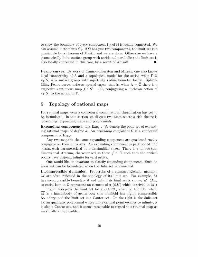
Figure 5 depicts the limit set for a Schottky group on the left, whereM is a handlebody of genus two; this manifold has highly compressibleboundary, and the limit set is a Cantor set. On the right is the Julia setfor an quadratic polynomial whose finite critical point escapes to infinity; Jis also a Cantor set, and it seems reasonable to regard this rational map asmaximally compressible.
20
Figure 5. Cantor sets
The classification of expanding components U is best understood in thecase of connected Julia sets — that is, the incompressible case.
Indeed, if J is connected then there is a unique f0 ∈ U , the center of U ,such that all critical points eventually map to periodic critical points. Themap f0 also forms the unique zero-dimensional Teichmuller stratum in U .Then a finite combinatorial invariant for U is the simply isotopy class [f0]of the branched covering
f0 : (S2, P (f0)) → (S2, P (f0)).
(Here P (f0) =⋃n>0,f ′
0(c)=0 f
n0 (c) is the postcritical set.)
Thurston’s combinatorial characterization of rational maps
• shows [f0] determines the rational map f0, and hence the expandingcomponent U of which it is the center, uniquely; and
• describes all branched coverings which can arise.
To state this theorem, let g : S2 → S2 be a topological branched coveringof degree d > 1. The map g is critically finite if |P (g)| < ∞, where P (g) isthe union of the forward orbits of the branch points.
Consider a finite system Γ of disjoint simple closed curves γ on S2−P (g),no two parallel, and none contractible or peripheral (i.e. enclosing a singlepoint of P (g)). The system Γ is g-invariant if every component α of g−1(γ)is contractible, peripheral or isotopic to some δ ∈ Γ. Define A(Γ) : RΓ → RΓ
by the formula
Aδγ =∑
α
1
deg(g : α→ γ)
21
where the sum is taken over components α of g−1(γ) which are isotopic toδ. Let λ(Γ) denote the spectral radius of Aδγ . Then we have:
Theorem 5.1 (Thurston) A critically finite branched cover g : S2 → S2
is realized by an expanding rational map f if and only if:
• every branch point of g eventually maps to a periodic branch point, and
• λ(Γ) < 1 for every g-invariant curve system Γ.
The rational map f is unique up to conformal conjugacy.
A slightly more general statement characterizes all critically finite (notnecessarily expanding) rational maps.
The fact that λ(Γ) < 1 for a rational map is already an interestingobservation. This can be seen by thickening the curves in Γ to annuli Cγ ,and observing that the geometry of P (f) gives an upper bound for thevector of conformal moduli [mγ ] = [mod(Cγ)]. The vector [Aδγmγ ] is astrict lower bound for the moduli of annuli which can be manufactured fromthe preimages of Cγ under f , so the Perron-Frobenius eigenvalue of Aδγ mustbe contracting.
Thurston’s criterion is rather implicit. Even fixing the degree d of g andthe size p = |P (g)| of the postcritical set, there are usually infinitely manyisotopy classes of branched coverings g, only finitely many of which representrational maps. For a more satisfactory classification, one needs to solve thefollowing combinatorial problem:
Problem 5.2 Find an efficient way to organize and enumerate all criticallyfinite rational maps of a given degree.
Acylindrical dynamics. A 3-manifold N with incompressible boundaryis acylindrical if any map f : (S1 × I, ∂(S1 × I)) → (N, ∂N), injective onπ1, is homotopic into ∂N . A compact Kleinian manifold M is acylindricalif and only if its limit set Λ is a Sierpinski curve. This means Λ is obtainedfrom the sphere by removing a countable dense set of open disks, boundedby disjoint Jordan curves whose diameters tend to zero.
Explicit examples of expanding rational maps with Sierpinski Julia setshave been given by Milnor-Tan and Pilgrim, and the notion of a “cylinder”for rational maps is under development.
Thurston showed that degeneration of Kleinian groups is related to cylin-ders, and that AH(π1(M )) is compact when M is acylindrical.
22
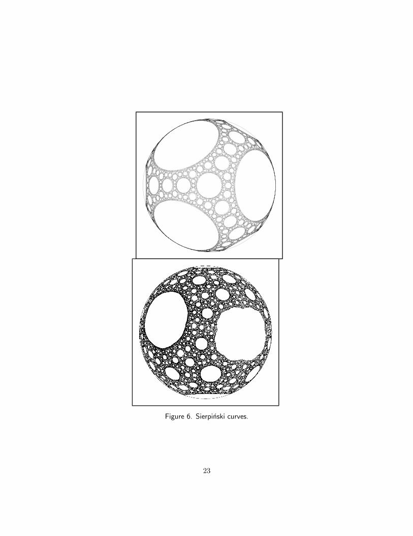
Figure 6. Sierpinski curves.
23
Question 5.3 Let U be an expanding component with center f0. If the Juliaset of f0 is a Sierpinski curve, is U ⊂ Vd compact?
At present, not one expanding component is known to have compactclosure.
Figure 6 depicts the limit set of an acylindrical Kleinian group above,and the Julia set of an acylindrical expanding rational map below. By aresult of Whyburn, these two fractal sets are homeomorphic.
A sequence of rational maps can degenerate by collapsing towards a mapof lower degree. Morgan and Shalen have used R-trees to study degenera-tions of hyperbolic manifolds, and Shishikura applied simplicial trees to somespecial degenerations of rational maps, so perhaps trees can help resolve thequestion above.
The general case. A compact 3-manifold with compressible boundary canbe cut along a finite number of compressing disks to obtain incompressiblepieces. Inverting this procedure, combination theorems of Klein and Maskitallow one to build up a Kleinian group with disconnected limit set from afinite number of subgroups with connected limit sets.
It should be possible to treat expanding rational maps with disconnectedJulia sets by an analogous procedure.
Problem 5.4 Develop decomposition and combination theorems for rationalmaps.
One would like a systematic theory including existing constructions likemating and tuning, as well a theory for disconnected Julia sets — just as theHaken theory discusses cutting along general incompressible subsurfaces, notjust disks. For example, some degree two rational maps can be expressedas matings in more than one way, just as a 3-manifold can contain severalembedded incompressible surfaces.
Problem 5.5 Give a combinatorial invariant for a general rational map f .
One expects that every Kleinian group is a limit of geometrically finitegroups of fixed topological type. In contrast to this, a rational map with everycycle repelling cannot belong to the closure of any expanding componentU ⊂ Vd. Thus it is challenging to predict even the topology of a sequence ofexpanding maps fn converging to f .
A combinatorial invariant for rational maps of degree two near a Lattesexample has been developed by Bernard.
24
Polynomials. Using laminations, one can formulate a combinatorial invari-ant for many polynomials.
Let f(z) = zd + a2zd−2 + . . . + ad be a monic centered polynomial of
degree d > 1 with connected Julia set. The set of all such polynomials formsthe connectedness locus Cd. The coefficients (a2, . . . , ad) of f determine anembedding of Cd as a compact, connected subset of Cd−1. Any polynomialwith connected Julia set is conformally conjugate to one in Cd.
The filled Julia set K(f) ⊂ C is the union of J(f) and the boundedcomponents of the Fatou set; it is compact set bounded by J(f). The com-plement C−K(f) is the basin of attraction of the point at infinity. By theRiemann mapping theorem, there is a unique conformal map
φf : (C−∆) → (C−K(f))
such that φf (z)/z → 1 as z → ∞. The map φf conjugates zd to f ; that is,that is, f(φf (z)) = φf (z
d).This conjugacy facilitates the encoding of the combinatorics of f by a
lamination. As can be seen in Figure 3, as f varies in Cd the topology ofthe Julia set J(f) can change from a circle to a circle with many pointsidentified. The lamination records these identifications.
Let S1 = R/Z, and identify S1 with the boundary of the unit disk ∆ viathe map t 7→ exp(2πit). For t ∈ S1, let
Rt = φf (r exp(2πit)) : 1 < r <∞
be the external ray at angle t. Clearly f(Rt) = Rdt. The ray Rt lands atp ∈ J(f) if
limrց1
φf (r exp(2πit)) = p.
It is known that Rt lands for every rational angle t, and if t is periodic undert 7→ dt, then the landing point p is a parabolic or repelling periodic pointfor f .
A lamination λ ⊂ S1×S1 is an equivalence relation such that the convexhulls of distinct equivalence classes are disjoint. The rational laminationλQ(f) is defined by t ∼ t′ if t = t′, or if t and t′ are rational and the externalrays Rt and Rt′ land at the same point in the Julia set J(f). (See Figure7 for an example where 1/7, 2/7, 4/17 is a single equivalence class underλQ(f).)
A map f ∈ Cd with no indifferent cycles is combinatorially rigid if it isdetermined up to quasiconformal conjugacy on its Julia set by its rational
25

Figure 7. External rays for f(z) = z2 + i.
lamination. More precisely, for any g ∈ Cd with no indifferent cycles suchthat λQ(g) = λQ(f), the conformal map
φg φ−1f : (C−K(f)) → (C−K(g))
should extend to a quasiconformal map on the whole Riemann sphere.We can now state:
Conjecture 5.6 (Combinatorial rigidity) Every polynomial with connectedJulia set and no indifferent cycle is combinatorially rigid.
One also conjectures a relative version of the density of expanding ratio-nal maps.
Conjecture 5.7 Expanding polynomials are dense in the connectedness lo-cus Cd and in the space of all polynomials of degree d.
Measure of Julia sets. A direct translation the Ahlfors measure zeroconjecture to the setting of rational maps appeared plausible for many years.Recently however the following result has been announced:
Theorem 5.8 (Nowicki-van Strien) Let d > 0 be an even integer, andlet f(z) = zd + c where c ∈ R. Suppose the closest returns of fn(0) to theorigin occur along the Fibonacci sequence n = 1, 2, 3, 5, 8, . . .. Then for dlarge enough, the Julia set of f has positive measure.
26

A pair of Fibonacci maps can also be combined to give a polynomialwhich is not ergodic on its Julia set. On the other hand, Ahlfors’ conjecturewas motivated by the problem of invariant complex structures on the limitset, and these Fibonacci maps carry no invariant line fields.
Question 5.9 When J(f) has positive measure, does it have finitely manyergodic components? Is their number bounded by the number of criticalpoints?
Though one expects the expanding maps to be open and dense in Vd,they do not fill out the space of rational maps in the sense of measure. Infact a random rational map has a definite chance of being ergodic:
Theorem 5.10 (Rees) The set of rational maps such that J(f) = C and facts ergodically on the sphere has positive measure in the space of all rationalmaps of degree d.
Local connectivity of Julia sets. If f ∈ Cd and its Julia set is locallyconnected, then J(f) is homeomorphic to S1/λ for some lamination λ. How-ever, it is known that there are Julia sets which are not locally connected. Aconcrete example is provided by f(z) = e2πitz + z2, where θ is an irrationalnumber which is very well approximated by rationals — e.g. t =
∑1/an
where a1, a2, a3, . . . = 2, 22, 222
, . . ..Expanding rational maps are better behaved. A rational map f is ge-
ometrically finite if every critical point either has a finite forward orbit, orconverges to an attracting, superattracting or parabolic cycle. Any expand-ing map is geometrically finite, and we have:
Theorem 5.11 (Tan-Yin) Every preperiodic component of the Julia set ofa geometrically finite rational map is locally connected.
6 Renormalization
Much progress towards the density of expanding dynamics and combinatorialrigidity has been recently achieved in the setting of quadratic polynomials.The methods also shed light on questions of local connectivity and measure.The very formulation of the results involves the idea of renormalization.
For quadratic polynomials Pc(z) = z2 + c, the connectedness locus C2 isthe same as the Mandelbrot set M ⊂ C. The Mandelbrot set can also bedescribed as the set of c such that Pnc (0) does not tend to infinity. By workof Douady, Hubbard and Yoccoz we have:
27

Theorem 6.1 Let c belong to the Mandelbrot set M . Then either
• Pc has an indifferent cycle and M is locally connected at c; or
• Pc has no indifferent cycle, and M is locally connected at c if and onlyif Pc is combinatorially rigid.
Corollary 6.2 (Douady-Hubbard) Local connectivity of the Mandelbrotset implies the density of expanding maps in the space of quadratic polyno-mials.
Proof. If M is locally connected then we have combinatorial rigidity indegree two.
Density of expanding dynamics can only fail if there is a component Qof int(M) consisting of a single quasiconformal conjugacy class, such thatf0 ∈ Q has all finite cycles repelling and an invariant line field on its Julia set.The points Bn ⊂ ∂Q with an indifferent cycle of period n are nowhere dense,so there is is a g ∈ ∂Q with no indifferent cycle. The rational laminationchanges only at parabolic points, so λQ(g) = λQ(f0).
Combinatorial rigidity would then imply g and f0 are quasiconformallyconjugate on their Julia sets. But then J(g) would carry an invariant linefield, contradicting the fact that g ∈ ∂M .
Figure 8. Small copies of M in M .
Quadratic-like maps. A remarkable feature of the Mandelbrot set is thatit contains countably many small copies of itself (Figure 8). To explain theseand other reappearances of M , Douady and Hubbard introduced the theory
28

of polynomial-like maps. A polynomial-like map f : U → V is a properholomorphic map between disks in the plane, such that U a compact subsetof V . The filled Julia set of f is defined by K(f) =
⋂∞1 f−n(V ), and the
Julia set J(f) is defined as its boundary. The filled Julia set consists of thepoints which never escape from the domain of f under iteration. A basictheorem asserts that f |K(f) is quasiconformally conjugate to p|K(p) forsome polynomial p.
Consider now a quadratic polynomial f(z) = z2+ c with connected Juliaset. A quadratic-like map is a polynomial-like map of degree two. We sayan iterate fn is renormalizable if there are disks Un and Vn, containing thecritical point z = 0, such that fn : Un → Vn is a quadratic-like map withconnected Julia set. (Note that fn itself has degree 2n.) If there are infinitelymany such n, then f is infinitely renormalizable.
A point s ∈ M is superstable of period p if z = 0 has period p underPs(z). Douady and Hubbard construct for each such s a tuning homeo-morphism M → Ms ⊂ M , written c 7→ s ∗ c, such that if c 6= 1/4, thenP ps∗c(z) is renormalizable and conjugate on its filled Julia set to Pc(z). Thusrenormalization explains the small copies of M inside of M . Any infinitelyrenormalizable map lies inside a countable nest of small Mandelbrot sets.
Example. The two left frames in Figure 9 depict the filled Julia sets offi(z) = z2 + si, i = 1, 2, where s1 and s2 are superstable of period two andthree respectively; the latter is known as Douady’s rabbit. The upper rightframe depicts the filled Julia set for f(z) = z2 + s1 ∗ s2; here the criticalpoint has period six, and f2 is renormalizable. The final frame shows thefilled Julia set of a renormalization f2 : U2 → V2; it is homeomorphic to therabbit.
We can now state two recent results towards the classification of quadraticpolynomials.
Theorem 6.3 (Yoccoz) Suppose c ∈ M and f(z) = z2 + c has no indif-ferent cycle. Then either:
• f is combinatorially rigid, J(f) is locally connected and M is locallyconnected at c, or
• f is infinitely renormalizable.
Theorem 6.4 (Lyubich) Combinatorial rigidity holds for uncountably manyinfinitely renormalizable quadratic polynomials f(z) = z2 + c with explicitlydescribed combinatorial classes.
29

Figure 9. Renormalization.
30

Carrying Yoccoz’s argument further, Lyubich and Shishikura proved in-dependently:
Theorem 6.5 If f(z) = z2 + c has no indifferent cycle and is only finiterenormalizable, then J(f) has measure zero.
Renormalization operators. Renormalization is closely related to uni-versality in dynamics.
To explain this phenomenon, for c ∈ M ∩ R = [−2, 1/4] let Ac ⊂ R
denote the set of accumulation points of Pnc (0). The set Ac often plays therole of an attractor for Pc over the reals; for example, it coincides with theattracting cycle if Pc has one.
Figure 10. Bifurcation diagram.
A classical experiment is to plot Ac as a function of c. Figure 10 rendersthe set (x, c) : x ∈ Ac,−0.6 < c < −2.0. Initially Ac is a single attractingfixed point; as c decreases (moving vertically in the figure), the attractorundergoes a sequence of period doublings, accumulating to a Cantor set atthe parameter cF ≈ −1.401155189. In physical terms cF marks a phase tran-sition from periodicity to chaos in this family. The Feigenbaum polynomialf(z) = z2 + cF is infinitely renormalizable; moreover the renormalization off2 is topologically conjugate to f itself.
In other families of real dynamical systems one finds cascades of perioddoublings remarkably similar to the quadratic family: for example the Haus-
31
dorff dimension of Ac and the pace of period doubling are independent ofthe particular family examined, and thus universal.
In the late 1970s Feigenbaum and Coullet-Tresser offered an explanationof this universality in terms of a fixed point for renormalization. Sullivan hasrecently given a rigorous proof of many aspects of this explanation; here isa precise statement in the language of quadratic-like mappings that followsfrom his work.
A quadratic-like map is real if f(z) = f(z). Let G denote the set ofreal quadratic-like maps f with connected Julia sets, up to affine conjugacynear K(f). We say [fn] → [f ] in G if there are representatives converginguniformly on a neighborhood of K(f). Let G(p) ⊂ G denote the set of f suchthat fp is renormalizable. The renormalization operator
Rp : G(p) → G
sends f to the germ of its quadratic-like restriction fp : Up → Vp. We maynow state:
Theorem 6.6 (Real fixed points of renormalization) Suppose the crit-ical point z = 0 has period p under z 7→ z2 + s, where s ∈ R. Then:
1. The limit s∞ = lim s∗n exists, and is the unique real fixed point oftuning by s;
2. if f(z) = z2 + s∞, then Rnp (f) → F , where F is a fixed-point of
renormalization; and
3. Rnp (g) → F for any g ∈ G which is topologically conjugate to f on
K(g) ∩R.
Corollary 6.7 The real fixed points of Rp are classified by the real super-stable points s ∈M of period p.
Example. For the Feigenbaum polynomial f(z) = z2 + cF , we have cF =(−1)∞, and after rescaling the renormalizations of f2
n
converge to a solutionF of the functional equation F F (z) = αF (α−1z).
3-manifolds which fiber over the circle. There is an intriguing analogybetween the renormalization operators and the mapping class group of asurface. Consider a closed surface S of genus 2 or more, and let ψ : S → Sbe a pseudo-Anosov mapping class. Then ψ acts on AH(π1(S)), and a
32
fixed point corresponds to a discrete faithful representation satisfying thefunctional equation
ρ ψ∗(γ) = α−1ρ(γ)α
for some α ∈ Aut(C). Although Γ = ρ(π1(S)) is geometrically infinite, thegroup generated by Γ and α is expanding, cocompact, and gives a hyper-bolic structure on the closed 3-manifold Tψ which fibers over the circle withmonodromy ψ.
Similarly, a fixed point for the renormalization operator Rp gives a solu-tion to the functional equation
F p(z) = α−1F (α(z)),
and while the critical point of F is recurrent, the dynamical system generatedby F and z 7→ αz has good expansion properties.
To complete the classification of quadratic polynomials, establish localconnectivity of the Mandelbrot and prove the density of expanding dynamics,it remains only to prove combinatorial rigidity in the infinitely renormaliz-able case. Although Theorem 6.4 handles many cases, even the following isstill open:
Question 6.8 Is the Feigenbaum polynomial combinatorially rigid?
Understanding the expansion implicit in renormalization may be usefulin resolving these questions.
7 Notes and references.
§1 Introduction. Classical references for conformal dynamical systems asseen by Poincare, Fatou and Julia include [Poin], [Julia], and [Fatou]. Thedictionary between rational maps and Kleinian groups was introduced in[Sul4] and is discussed at length in [Sul2]. The scope of conformal dynamicsis broader than our focus here; it includes real one-dimensional dynamicsand codimension-one holomorphic foliations, as well iterated entire functions,correspondences, and higher-dimensional Kleinian groups.
§2 Finiteness theorems and Teichmuller space. Ahlfors’ finitenesstheorem and the Ahlfors measure zero problem appear in [Ah]; the numberof triply-punctured spheres is bounded in [Gre]. Sullivan’s no wanderingdomains theorem appears in [Sul4] (see also [Bers3]), and the Teichmullerspace of a holomorphic dynamical system is developed in [McS]. Bers’ areatheorem and Shishikura’s bounds are in [Bers1] and [Shi1].
33

§3 Expanding dynamics. A candidate 3-dimensional object for a rationalmaps is constructed in [LM]. A prototype for the conjecture on the densityof convex cocompact groups is [Bers2, Conjecture II].
The relation of hyperbolicity to structural stability is discussed for Kleiniangroups in [Sul5], and for rational maps in [MSS], [McS] and [Mc4]. Theorem3.6 and its Corollary can be found in [McS].
Density of hyperbolicity has been announced for the family of entirefunctions fλ(z) = λ tan z [KK].
§4 Topology of hyperbolic 3-manifolds. Marden’s work on the topologyof geometrically finite 3-manifolds appears in [Mrd]. The basic referencefor the ending lamination, pleated surfaces, topological tameness and theirrelation to the Ahlfors conjecture is [Th1]. Important further developmentsappear in [Bon], [Oh], [Min1], [Can] and [Min2]. The Whitehead continuum(whose complement gives a manifold with a wild end) is discussed in [Rol,§3I].
Thurston’s geometrization theorem for Haken manifolds is discussed in[Mor1], [Th2] and [Th3]; a new approach to the the proof is surveyed in[Mc3].
The Hausdorff dimension of limit sets is studied in [Sul1], [Sul3], [Tu]and [BJ].
The local connectivity of geometrically finite limit sets (Theorem 4.18)is assembled from [AM], [Msk2, Theorem 6], [Msk1, Theorem 2] and [Ab,Theorem 3]; see also [Fl]. A more detailed proof is given in [AM]. EquivariantPeano curves are discussed in [Th2] and [CT]; [Min1] contains more generallocal connectivity results.
§5 Topology of rational maps. Thurston’s characterization of criti-cally finite rational maps appears in [Th4], [DH2]; it is compared to thegeometrization of 3-manifolds in [Mc2]. The problem of enumerating crit-ically finite polynomials is addressed in [BFH] and [Po]; [Rs2] studies thecombinatorics of rational maps of degree two.
Sierpinski Julia sets and components of the space of expanding mapsare discussed in [Mc1, §4] (which includes a version of Question 5.3), [Mil2],[Pil], [Mak] and [Pet]. Sierpinski’s curve first appears in [Sie]; its uniquenessis proved in [Why]. For the role of trees in conformal dynamics, see [Mor2],[Shi2].
Tuning, mating and other surgery constructions can be found in [Dou1]and [Tan]. Combinatorics near a degree two Lattes example is developed in[Ber].
The landing of external rays is discussed in [Mil3, §18], [Hub] and [Mc4,
34

§6]. A proof that Cd cellular, and therefore connected, appears in [Lav].A polynomial Julia set of positive measure is constructed in [NS], and
an example which is not ergodic on its Julia set appears in [vS]. Positivemeasure sets of ergodic maps are constructed in [Rs1].
For local connectivity of geometrically finite Julia sets, see [TY].
§6 Renormalization. External angles for Julia sets and the Mandelbrotset are studied in [DH1], which includes a proof that local connectivity ofM implies the density of expanding polynomials. A more recent treatmentappears in [Dou2]. See [Mil1] for the tuning operators and self-similarity ofthe Mandelbrot set.
Background on complex renormalization can be found in [Mc4]; for a his-torical collection including experimental work on physical systems, see [Cvi].Work of Yoccoz on the local connectivity of J(f) and M is presented in [Y],[Mil4] and [Hub]. These breakthroughs were foreshadowed by work of Bran-ner and Hubbard on cubic polynomials with disconnected Julia sets [BH].Theorem 6.5 on the measure of Julia sets appears in [Ly2]. For Lyubich’sresults on infinitely renormalizable quadratic polynomials, see [Ly1].
Sullivan’s work on renormalization appears in [Sul6], and is expandedupon in [MeSt]. A parallel approach to renormalization and 3-manifoldswhich fiber over the circle is the subject of [Mc5]. Theorem 6.6 is implicitin Sullivan’s work and stated explicitly in [Mc5, Thm 7.16].
The illustrations. Figure 2 and the left frame of Figure 5 were drawn us-ing a computer program written by David Wright [MMW]. The remainingpictures were produced by the author. In Figure 6, the Kleinian group isgenerated by reflections through the sides of a regular stunted ideal tetrahe-dron with dihedral angles 2π/7; the rational map is f(z) ≈ −0.695620(z −1)2(z + 2)/(3z − 2). The second frame of Figure 8 is a blowup around c ≈−0.160 + 1.034i, a superstable point of period 4. The parameters for Figure9 are s1 = −1, s2 ≈ −0.22561+0.744862i and s1 ∗s2 ≈ −1.13000+0.24033i.
References
[Ab] W. Abikoff. On boundaries of Teichmuller spaces and on Kleiniangroups: III. Acta Math. 134(1975), 211–237.
[AM] W. Abikoff and B. Maskit. Geometric decompositions of Kleiniangroups. Amer. J. Math 99(1977), 687–698.
[Ah] L. Ahlfors. Finitely generated Kleinian groups. Amer. J. of Math.86(1964), 413–429.
35
[AM] J. Anderson and B. Maskit. On the local connectivity of limitsets of Kleinian groups. Complex Variables Theory Appl. 31(1996),177–183.
[Ber] J. Bernard. Dynamique des perturbations d’un example de Lattes.Thesis, Univ. Paris-Sud Orsay, 1994.
[Bers1] L. Bers. Inequalities for finitely generated Kleinian groups. J.d’Analyse Math. 18(1967), 23–41.
[Bers2] L. Bers. On boundaries of Teichmuller spaces and on kleiniangroups: I. Annals of Math. 91(1970), 570–600.
[Bers3] L. Bers. On Sullivan’s proof of the finiteness theorem and theeventual periodicity theorem. Am. J. Math. 109(1987), 833–852.
[BFH] Bielefeld, Y. Fisher, and J. Hubbard. The classification of criticallypreperiodic polynomials as dynamical systems. J. Amer. Math. Soc.5(1992), 721–762.
[BJ] C. J. Bishop and P. W. Jones. Hausdorff dimension and Kleiniangroups. Acta Math. 179(1997), 1–39.
[Bon] F. Bonahon. Bouts des varietes hyperboliques de dimension 3. An-nals of Math. 124(1986), 71–158.
[BH] B. Branner and J. H. Hubbard. The iteration of cubic polynomials,Part II: Patterns and parapatterns. Acta Math. 169(1992), 229–325.
[Can] R. D. Canary. Ends of hyperbolic 3-manifolds. J. Amer. Math. Soc.6(1993), 1–35.
[CT] J. W. Cannon and W. P. Thurston. Group invariant Peano curves.Preprint, Princeton, 1985.
[Cvi] P. Cvitanovic. Universality in Chaos. Adam Hilger Ltd, 1984.
[Dou1] A. Douady. Chirurgie sur les applications holomorphes. In Proceed-ings of the International Congress of Mathematicians (Berkeley,1986), pages 724–738. Amer. Math. Soc., 1986.
[Dou2] A. Douady. Descriptions of compact sets in C. In L. R. Goldbergand A. V. Phillips, editors, Topological Methods in Modern Mathe-matics, pages 429–465. Publish or Perish, Inc., 1993.
36
[DH1] A. Douady and J. Hubbard. Etude dynamique des polynomes com-plexes. Pub. Math. d’Orsay 84–2, 85–4, 1985.
[DH2] A. Douady and J. Hubbard. A proof of Thurston’s topologicalcharacterization of rational maps. Acta Math. 171(1993), 263–297.
[Fatou] P. Fatou. Sur les equations fonctionnelles. Bull. Sci. Math. France47–48(1919–20), 161–271, 33–94, 208–314.
[Fl] W. J. Floyd. Group completions and limit sets of Kleinian groups.Invent. math. 57(1980), 205–218.
[Gre] L. Greenberg. On a theorem of Ahlfors and conjugate subgroups ofKleinian groups. Amer. J. Math 89(1967), 56–68.
[Hub] J. H. Hubbard. Local connectivity of Julia sets and bifurcationloci: three theorems of J.-C. Yoccoz. In L. R. Goldberg andA. V. Phillips, editors, Topological Methods in Modern Mathemat-ics, pages 467–511. Publish or Perish, Inc., 1993.
[Julia] G. Julia. Memoire sur l’iteration des applications fonctionnelles. J.Math. Pures et Appl. 8(1918), 47–245.
[KK] L. Keen and J. Kotus. Dynamics of the family λ tan z. Preprint,1994.
[Lav] P. Lavaurs. Systemes dynamiques holomorphes: explosion de pointsperiodiques paraboliques. Thesis, Univ. Paris-Sud Orsay, 1989.
[Ly1] M. Lyubich. Geometry of quadratic polynomials: Moduli, rigidity,and local connectivity. Stony Brook IMS Preprint 1993/9.
[Ly2] M. Lyubich. On the Lebesgue measure of the Julia set of a quadraticpolynomial. Stony Brook IMS Preprint 1991/10.
[LM] M. Lyubich and Y. Minsky. Laminations in holomorphic dynamics.J. Diff. Geom. 47(1997), 17–94.
[Mak] P. Makienko. Unbounded components in parameter space of ratio-nal maps. ICTP Trieste Preprint IC/93–84.
[MSS] R. Mane, P. Sad, and D. Sullivan. On the dynamics of rationalmaps. Ann. Sci. Ec. Norm. Sup. 16(1983), 193–217.
37

[Mrd] A. Marden. The geometry of finitely generated kleinian groups.Annals of Math. 99(1974), 383–462.
[Msk1] B. Maskit. On boundaries of Teichmuller spaces and on kleiniangroups: II. Annals of Math. 91(1970), 607–639.
[Msk2] B. Maskit. Intersection of component subgroups of Kleinian groups.In Discontinuous Groups and Riemann Surfaces, volume 79 of An-nals of Math. Studies, pages 349–367. Princeton University Press,1974.
[Mc1] C. McMullen. Automorphisms of rational maps. In HolomorphicFunctions and Moduli I, pages 31–60. Springer-Verlag, 1988.
[Mc2] C. McMullen. Rational maps and Kleinian groups. In Proceedingsof the International Congress of Mathematicians (Kyoto, 1990),pages 889–900. Springer-Verlag, 1991.
[Mc3] C. McMullen. Riemann surfaces and the geometrization of 3-manifolds. Bull. Amer. Math. Soc. 27(1992), 207–216.
[Mc4] C. McMullen. Complex Dynamics and Renormalization, volume135 of Annals of Math. Studies. Princeton University Press, 1994.
[Mc5] C. McMullen. Renormalization and 3-Manifolds which Fiber overthe Circle, volume 142 of Annals of Math. Studies. Princeton Uni-versity Press, 1996.
[McS] C. McMullen and D. Sullivan. Quasiconformal homeomorphismsand dynamics III: The Teichmuller space of a holomorphic dynam-ical system. Adv. Math. 135(1998), 351–395.
[MeSt] W. de Melo and S. van Strien. One-Dimensional Dynamics.Springer-Verlag, 1993.
[Mil1] J. Milnor. Self-similarity and hairiness in the Mandelbrot set. InM. C. Tangora, editor, Computers in Geometry and Topology, Lect.Notes Pure Appl. Math., pages 211–259. Dekker, 1989.
[Mil2] J. Milnor. Geometry and dynamics of quadratic rational maps.Experiment. Math. 2(1993), 37–83.
[Mil3] J. Milnor. Dynamics in One Complex Variable: Introductory Lec-tures. Vieweg, 1999.
38
[Mil4] J. Milnor. Local connectivity of Julia sets: expository lectures. InTan Lei, editor, The Mandelbrot Set, Theme and Variations, pages67–116. Cambridge University Press, 2000.
[Min1] Y. Minsky. On rigidity, limit sets, and end invariants of hyperbolic3-manifolds. J. Amer. Math. Soc. 7(1994), 539–588.
[Min2] Y. Minsky. The classification of punctured torus groups. Annals ofMath. 149(1999), 559–626.
[Mor1] J. Morgan. On Thurston’s uniformization theorem for three dimen-sional manifolds. In The Smith Conjecture, pages 37–125. AcademicPress, 1984.
[Mor2] J. Morgan. Trees and hyperbolic geometry. In Proceedings of theInternational Congress of Mathematicians (Berkeley, 1986), pages590–597. Amer. Math. Soc., 1987.
[MMW] D. Mumford, C. McMullen, and D. Wright. Limit sets of free two-generator kleinian groups. Preprint, 1990.
[NS] T. Nowicki and S. van Strien. Polynomial maps with a Julia set ofpositive Lebesgue measure: Fibonacci maps. Preprint, 1993.
[Oh] K. Ohshika. Ending laminations and boundaries for deformationspaces of Kleinian groups. J. London Math. Soc. 42(1990), 111–121.
[Pet] C. L. Petersen. No elliptic limits for quadratic maps. Preprint,MAT-Report No. 1994–45.
[Pil] K. Pilgrim. Cylinders for Iterated Rational Maps. Thesis, Univer-sity of California, Berkeley, 1994.
[Poin] H. Poincare. Memoire sur les groupes kleineens. Acta Math.3(1883), 49–92.
[Po] A. Poirier. On post critically finite polynomials, Part two: Hubbardtrees. Stony Brook IMS Preprint 1993/5.
[Rs1] M. Rees. Positive measure sets of ergodic rational maps. Ann.scient. Ec. Norm. Sup. 19(1986), 383–407.
[Rs2] M. Rees. A partial description of parameter space of rational mapsof degree two: Part I. Acta Math. 168(1992), 11–87.
39

[Rol] D. Rolfsen. Knots and Links. Publish or Perish, Inc., 1976.
[Shi1] M. Shishikura. On the quasiconformal surgery of rational functions.Ann. Sci. Ec. Norm. Sup. 20(1987), 1–30.
[Shi2] M. Shishikura. Trees associated with the configuration of Hermanrings. Ergod. Th. & Dynam. Sys. 9(1989), 543–560.
[Sie] W. Sierpinski. Sur une courbe cantorienne qui contient une im-age biunivoque et continue de toute courbe donnee. In OeuvresChoisies, t. II, pages 107–119. PWN – Editions sci. de Pologne,1975.
[vS] S. van Strien. Transitive maps which are not ergodic with respectto Lebesgue measure. Preprint, 1995.
[Sul1] D. Sullivan. Growth of positive harmonic functions and Kleiniangroup limit sets of zero planar measure and Hausdorff dimensiontwo. In Geometry at Utrecht, volume 894 of Lecture Notes in Math.,pages 127–144. Springer, 1981.
[Sul2] D. Sullivan. Conformal dynamical systems. In Geometric Dy-namics, volume 1007 of Lecture Notes in Math., pages 725–752.Springer, 1983.
[Sul3] D. Sullivan. Entropy, Hausdorff measures new and old and limitsets of geometrically finite Kleinian groups. Acta Math. 153(1984),259–277.
[Sul4] D. Sullivan. Quasiconformal homeomorphisms and dynamics I: So-lution of the Fatou-Julia problem on wandering domains. Annalsof Math. 122(1985), 401–418.
[Sul5] D. Sullivan. Quasiconformal homeomorphisms and dynamics II:Structural stability implies hyperbolicity for Kleinian groups. ActaMath. 155(1985), 243–260.
[Sul6] D. Sullivan. Bounds, quadratic differentials and renormalizationconjectures. In F. Browder, editor, Mathematics into the Twenty-first Century: 1988 Centennial Symposium, August 8–12, pages417–466. Amer. Math. Soc., 1992.
[Tan] Tan L. Matings of quadratic polynomials. Ergod. Th. & Dynam.Sys. 12(1992), 589–620.
40

[TY] Tan L. and Yin Y. Local connectivity of the Julia set for geomet-rically finite rational maps. Science in China (Series A) 39(1996),39–47.
[Th1] W. P. Thurston. Geometry and Topology of Three-Manifolds. Lec-ture Notes, Princeton University, 1979.
[Th2] W. P. Thurston. Three-dimensional manifolds, Kleinian groups andhyperbolic geometry. Bull. Amer. Math. Soc. 6(1982), 357–381.
[Th3] W. P. Thurston. Hyperbolic structures on 3-manifolds I: Deforma-tions of acylindrical manifolds. Annals of Math. 124(1986), 203–246.
[Th4] W. P. Thurston. On the combinatorics and dynamics of iteratedrational maps. Preprint.
[Tu] P. Tukia. The Hausdorff dimension of the limit set of a geometricallyfinite Kleinian group. Acta Math. 152(1984), 127–140.
[Why] G. T. Whyburn. Topological characterization of the Sierpinskicurve. Fund. Math. 45(1958), 320–324.
[Y] J.-C. Yoccoz. Sur la connexite locale des ensembles de Julia et dulieu de connexite des polynomes. In preparation.
41

![4d N =2SCFT from complete intersection singularity...802 Y.-F. Wang, et al. torus [48], one can derive the classification of four dimensional N =4super- conformal field theories](https://static.fdocuments.us/doc/165x107/614a775c12c9616cbc696f18/4d-n-2scft-from-complete-intersection-singularity-802-y-f-wang-et-al-torus.jpg)


![ASYMPTOTIC COUNTING CONFORMAL DYNAMICAL SYSTEMScounting problems in geometry and dynamics has been used by several authors including [42], [35], [48], [3]. We now discuss our results](https://static.fdocuments.us/doc/165x107/5f646bac117949352e721664/asymptotic-counting-conformal-dynamical-systems-counting-problems-in-geometry-and.jpg)