The classical Bloch equations

Martin Frimmer and Lukas NovotnyETH Z€urich, Photonics Laboratory, 8093 Z€urich, Switzerland (www.photonics.ethz.ch)

(Received 13 October 2013; accepted 7 May 2014)

Coherent control of a quantum mechanical two-level system is at the heart of magnetic resonance

imaging, quantum information processing, and quantum optics. Among the most prominent

phenomena in quantum coherent control are Rabi oscillations, Ramsey fringes, and Hahn echoes.

We demonstrate that these phenomena can be derived classically by use of a simple coupled-

harmonic-oscillator model. The classical problem can be cast in a form that is formally

equivalent to the quantum mechanical Bloch equations with the exception that the longitudinal

and the transverse relaxation times (T1 and T2) are equal. The classical analysis is intuitive and

well suited for familiarizing students with the basic concepts of quantum coherent control, while

at the same time highlighting the fundamental differences between classical and quantum

theories. VC 2014 American Association of Physics Teachers.

[http://dx.doi.org/10.1119/1.4878621]

I. INTRODUCTION

The harmonic oscillator is arguably the most fundamentalbuilding block at the core of our understanding of both clas-sical and quantum physics. Interestingly, a host of phenom-ena originally encountered in quantum mechanics andinitially thought to be of purely quantum-mechanical naturehave been successfully modelled using coupled classical har-monic oscillators. Among these phenomena are electromag-netically induced transparency,1 rapid adiabatic passage,2,3

and Landau-Zener tunneling.4 A particularly rich subset ofexperiments is enabled by the coherent manipulation of aquantum-mechanical two-level system, providing access tofascinating effects including Rabi oscillations, Ramseyfringes, and Hahn echoes.5 Remarkably, equipped with themodels and ideas gained from studying quantum-mechanicalsystems, researchers have returned to construct classical ana-logues of two-level systems.6,7 Coherent control of such aclassical two-level system has been beautifully demonstratedfor an “optical atom” consisting of two coupled modes of acavity.8,9 Recently, coherent control of classical two-levelsystems has been achieved with coupled micromechanicaloscillators.10,11 With the analogy between a two-level systemand a coupled pair of classical harmonic oscillators wellestablished, it is surprising that this analogy has not beenused to familiarize students with the concepts of coherentcontrol and to provide an accessible analogue to a variety ofquantum optical phenomena. Furthermore, exploring the lim-its of any analogue typically illustrates very strikingly thegenuine features of a physical theory that are not present inthe theory in which the analogy is phrased.12

In this paper, we consider a pair of two parametricallydriven coupled mechanical (harmonic) oscillators. FromNewton’s second law, we derive a set of equations of motionfor the eigenmode amplitudes that are formally equivalent tothe time-dependent Schr€odinger equation of a two-levelatom. We then derive a set of coupled differential equationsthat are formally identical with the quantum Bloch equa-tions, with the exception that the longitudinal and transverserelaxation times are equal. We illustrate the concept of theBloch sphere and provide an intuitive understanding ofcoherent control experiments by discussing Rabi oscillations,Ramsey fringes, and Hahn echoes. Finally, we point out thedistinct differences between our mechanical analogue and atrue quantum-mechanical two-level system. Our approach

offers students an intuitive entry into the field and preparesthem with the basic concepts of quantum coherent control.

II. THE MECHANICAL ATOM

A. Equations of motion

Throughout this paper, we consider two oscillators, asillustrated in Fig. 1, with masses mA and mB, spring constantskA¼ k – Dk(t) and kB¼ k þ Dk(t) with a small detuning Dk(t)that can be time dependent, and coupled by a spring withspring constant j, which is weak compared to k. Oscillator Acan be externally driven by a force F(t), and both oscillatorsare weakly damped at a rate c. Because of the coupling j, thedynamics of oscillator A couples over to oscillator B. Suchtwo coupled harmonic oscillators are a generic model systemapplicable to diverse fields of physics. For example, in molec-ular physics oscillators A and B correspond to a pair of atoms.Similarly, in cavity quantum electrodynamics, A is a two-level atom and B is a cavity field. In cavity optomechanics,oscillator A would represent a mechanical oscillator, such asa membrane or cantilever, and B an optical resonator. For thefollowing, we assume that the masses of the oscillators areequal (mA¼mB¼m). Then, in terms of the coordinates xA

and xB of the two oscillators, the equations of motion are

€xA þ c _xA þk þ j

m� DkðtÞ

m

� �xA �

jm

xB ¼FðtÞm

;

€xB þ c _xB þk þ j

mþ DkðtÞ

m

� �xB �

jm

xA ¼ 0:

(1)

Fig. 1. Coupled mechanical oscillators with masses mA, mB and spring con-

stants kA¼ k – Dk, kB¼ k þ Dk with a detuning Dk that can be time depend-

ent. Oscillator A can be driven by an external force F(t), and the oscillators

are coupled with a spring (with spring constant j).

947 Am. J. Phys. 82 (10), October 2014 http://aapt.org/ajp VC 2014 American Association of Physics Teachers 947

For ease of notation, we introduce the carrier frequency X0, thedetuning frequency Xd, and the coupling frequency Xc as

X20 ¼

k þ jm

;

X2d ¼

Dk

m;

X2c ¼

jm;

(2)

and represent the coupled differential equations in Eq. (1) inmatrix form as

d2

dt2þ c

d

dtþX2

0

� �xA

xB

" #þ �X2

d �X2c

�X2c X2

d

" #xA

xB

" #¼

f ðtÞ0

" #;

(3)

where f(t)¼F(t)/m. This system of equations describes thefull dynamics of the coupled oscillator problem.

B. Eigenmodes for constant detuning

We first consider the case of constant detuning(Dk¼ constant) and solve for the eigenmodes of the systemand their respective eigenfrequencies. To this end, we diago-nalize the matrix in Eq. (3). The eigenmodes xe1 and xe2 ofthe system can be derived from the coordinates of the twooscillators xA and xB as

xA

xB

� �¼ U�1 xe1

xe2

� �; (4)

where U is a transformation matrix, whose rows are theeigenvectors of the matrix in Eq. (3). We find

U ¼ U11 U12

U21 U22

� �

¼1 �ðXd=XcÞ2 þ

ffiffiffiffiffiffiffiffiffiffiffiffiffiffiffiffiffiffiffiffiffiffiffiffiffiffiffi1þ ðXd=XcÞ4

q1 �ðXd=XcÞ2 �

ffiffiffiffiffiffiffiffiffiffiffiffiffiffiffiffiffiffiffiffiffiffiffiffiffiffiffi1þ ðXd=XcÞ4

q264

375; (5)

and the eigenfrequencies turn out to be

X6 ¼ X20 7

ffiffiffiffiffiffiffiffiffiffiffiffiffiffiffiffiffiX4

d þ X4c

q� �1=2

: (6)

Here, Xþ denotes the frequency of the symmetric eigen-mode, which is lower than the frequency X– of the antisym-metric eigenmode. Thus, after transformation, Eq. (3) yieldstwo independent differential equations for the normal modecoordinates xe1 and xe2:

d2

dt2þ c

d

dtþ X2

þ

� �xe1 ¼ U11f ðtÞ

d2

dt2þ c

d

dtþ X2

�

� �xe2 ¼ U21f ðtÞ:

(7)

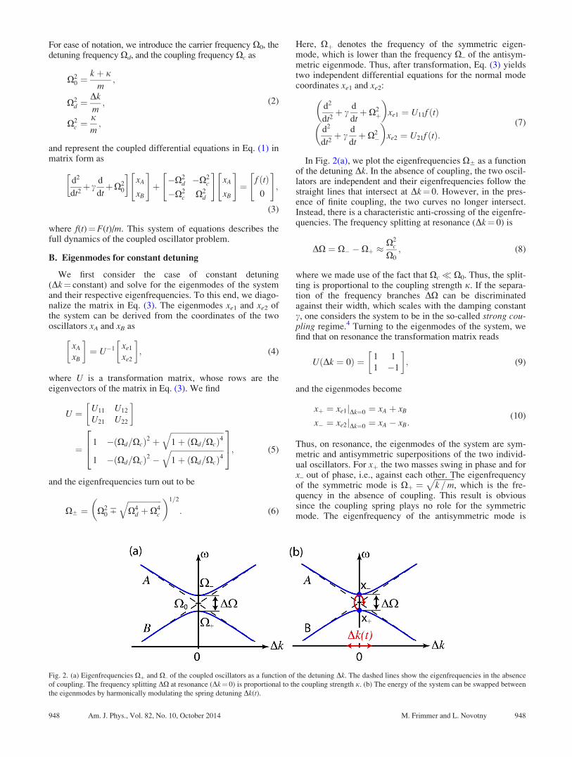
In Fig. 2(a), we plot the eigenfrequencies X6 as a functionof the detuning Dk. In the absence of coupling, the two oscil-lators are independent and their eigenfrequencies follow thestraight lines that intersect at Dk¼ 0. However, in the pres-ence of finite coupling, the two curves no longer intersect.Instead, there is a characteristic anti-crossing of the eigenfre-quencies. The frequency splitting at resonance (Dk¼ 0) is

DX ¼ X� � Xþ �X2

c

X0

; (8)

where we made use of the fact that Xc� X0. Thus, the split-ting is proportional to the coupling strength j. If the separa-tion of the frequency branches DX can be discriminatedagainst their width, which scales with the damping constantc, one considers the system to be in the so-called strong cou-pling regime.4 Turning to the eigenmodes of the system, wefind that on resonance the transformation matrix reads

UðDk ¼ 0Þ ¼ 1 1

1 �1

� �; (9)

and the eigenmodes become

xþ ¼ xe1jDk¼0 ¼ xA þ xB

x� ¼ xe2jDk¼0 ¼ xA � xB:(10)

Thus, on resonance, the eigenmodes of the system are sym-metric and antisymmetric superpositions of the two individ-ual oscillators. For xþ the two masses swing in phase and forx– out of phase, i.e., against each other. The eigenfrequencyof the symmetric mode is Xþ ¼

ffiffiffiffiffiffiffiffiffiffik =m

p, which is the fre-

quency in the absence of coupling. This result is obvioussince the coupling spring plays no role for the symmetricmode. The eigenfrequency of the antisymmetric mode is

Fig. 2. (a) Eigenfrequencies Xþ and X– of the coupled oscillators as a function of the detuning Dk. The dashed lines show the eigenfrequencies in the absence

of coupling. The frequency splitting DX at resonance (Dk¼ 0) is proportional to the coupling strength j. (b) The energy of the system can be swapped between

the eigenmodes by harmonically modulating the spring detuning Dk(t).

948 Am. J. Phys., Vol. 82, No. 10, October 2014 M. Frimmer and L. Novotny 948

X� ¼ffiffiffiffiffiffiffiffiffiffiffiffiffiffiffiffiffiffiffiffiffiffiffiffiffiðk þ 2jÞ =m

p. This frequency is higher than Xþ

because each oscillator feels the coupling spring.We have thus far considered a static detuning Dk.

Intriguing effects happen when Dk becomes time dependent.For example, if oscillator A is excited and the detuning Dk isswept through the anti-crossing region, then, depending onhow fast the parameter Dk is varied, one can transfer theenergy to oscillator B or keep it in oscillator A. The former isreferred to as an adiabatic transition and the latter as a dia-batic transition. In a diabatic transition, the system jumpsfrom one branch in Fig. 2(a) to the other, a process referredto as a Landau-Zener transition.4,9 In this paper, instead oflinearly sweeping Dk, we consider a detuning that varies har-monically in time. Before doing this, we introduce the slowlyvarying envelope approximation to establish the formal cor-respondence between the mechanical oscillator system and aquantum mechanical two-level system.

C. The slowly varying envelope approximation

We are interested in the dynamics of the coupled oscilla-tors when they are tuned close to resonance (Dk¼ 0).Therefore, we transform Eq. (3) to the (xþ, x–) basis andobtain

d2

dt2þ c

d

dtþX2

0

� �xþx�

� �þ �X2

c �X2d

�X2d X2

c

" #xþ

x�

" #¼

f ðtÞf ðtÞ

" #;

(11)

where we have used the transformation matrix U(Dk¼ 0)given in Eq. (9). Note that the transformation to the (reso-nant) eigenmodes has interchanged the roles of detuning andcoupling in the matrix in Eq. (11) as compared to Eq. (3). Adriving force f(t) can be used to excite the system in anyeigenmode or superposition of eigenmodes. However, sincewe are interested in the dynamics of the system after its initi-alization, we will from now on set f(t)¼ 0.

To understand the evolution of the eigenmodes we write

xþ ¼ Re aðtÞeiX0t� �

x� ¼ Re bðtÞeiX0t� �

;(12)

where each mode is rapidly oscillating at the carrier fre-quency X0 and modulated by the slowly varying complexamplitudes a(t) and b(t). Upon inserting Eq. (12) into thecoupled equations of motion (11), we assume that the ampli-tude functions a(t) and b(t) do not change appreciably duringan oscillation period 2p/X0, which allows us to neglect termscontaining second time derivatives. This procedure is calledthe slowly varying envelope approximation (SVEA).Furthermore, since we consider weak damping, we use 2iX0

þ c � 2iX0. With these approximations, we arrive at the fol-lowing equations of motion for the eigenmode amplitudes

i_a_b

� �¼ 1

2

DX� ic xd

xd �DX� ic

� �ab

� �: (13)

To simplify notation, we have introduced the rescaled detun-ing frequency

xd ¼X2

d

X0

: (14)

Note that, for the case of vanishing damping (c¼ 0), Eq. (13)resembles the time dependent Schr€odinger equationi�h @tjWi ¼ H jWi for a state vector jWi ¼ aðtÞjgi þ bðtÞjei;that is, a superposition of a ground state jgi and an excitedstate jei separated in energy by �hDX. The two states arecoupled by hejH jgi ¼ �hxd=2. Accordingly, our system ofcoupled harmonic oscillators can be considered as a“mechanical atom,” whose ground state (excited state) isrepresented by the symmetric eigenmode xþ (antisymmetriceigenmode x–). Importantly, the detuning Dk of the oscilla-tors leads to a coupling of the eigenmodes xþ and x–.

D. Parametrically driven system

We now investigate the dynamics of the “mechanicalatom” for a time harmonic detuning

DkðtÞ ¼ �2X0mA cosðxdrivetÞ; (15)

such that xd ¼ �A expðixdrivetÞ þ expð�ixdrivetÞ½ �. The am-plitude A corresponds to the magnitude of the external mod-ulation, whereas xdrive is the frequency of the modulation(c.f. Fig. 1). To ease the notation, we apply thetransformation

a ¼ �aðtÞe�ixdrivet=2;b ¼ �bðtÞeþixdrivet=2:

(16)

Here, �a and �b are the slowly varying amplitudes of the sym-metric and antisymmetric eigenmodes in a coordinate framerotating at the driving frequency. This transformation gener-ates terms exp½63ixdrivet=2� in Eq. (13) that are rapidlyoscillating and that we neglect because they average out onthe time scales of interest. This approximation is commonlyreferred to as the rotating wave approximation (RWA).5 Inthe RWA and after transformation into the rotating coordi-nate frame Eq. (13) reads

i_�a_�b

" #¼ 1

2

d� ic �A�A �d� ic

� ��a�b

� �; (17)

where we have defined the detuning d between the drivingfrequency and the level splitting

d ¼ DX� xdrive: (18)

Note that the RWA and the transformation into a rotatingcoordinate frame have turned the problem of two parametri-cally driven modes into a simple problem of two modes witha static coupling. With the initial conditions �aðt ¼ 0Þ ¼ �a0

and �bðt ¼ 0Þ ¼ �b0 the solutions of Eq. (17) are

�aðtÞ ¼

iA

XRsin

XRt

2

� ��b0

þ cosXRt

2

� �� i

dXR

sinXRt

2

� �� ��a0

e�ct=2;

�bðtÞ ¼

iA

XRsin

XRt

2

� ��a0

þ cosXRt

2

� �þ i

dXR

sinXRt

2

� �� ��b0

e�ct=2;

(19)

949 Am. J. Phys., Vol. 82, No. 10, October 2014 M. Frimmer and L. Novotny 949

where we have introduced the generalized Rabi-frequency

XR ¼ffiffiffiffiffiffiffiffiffiffiffiffiffiffiffiffiA2 þ d2

p: (20)

Equations (19) together with Eqs. (10), (12), and (16) are thegeneral solutions to the problem of two coupled harmonicoscillators under a time harmonic detuning. Note that oursolutions rely on the validity of the RWA, which is reflectedby the fact that Eq. (19) only retains dynamics on the timescale given by the generalized Rabi-frequency XR, andneglects any fast dynamics on time scales set by xdrive.Accordingly, our solutions are only valid for driving ampli-tudes A and detunings d small enough to ensure XR� xdrive.

E. The Bloch sphere and the Bloch equations

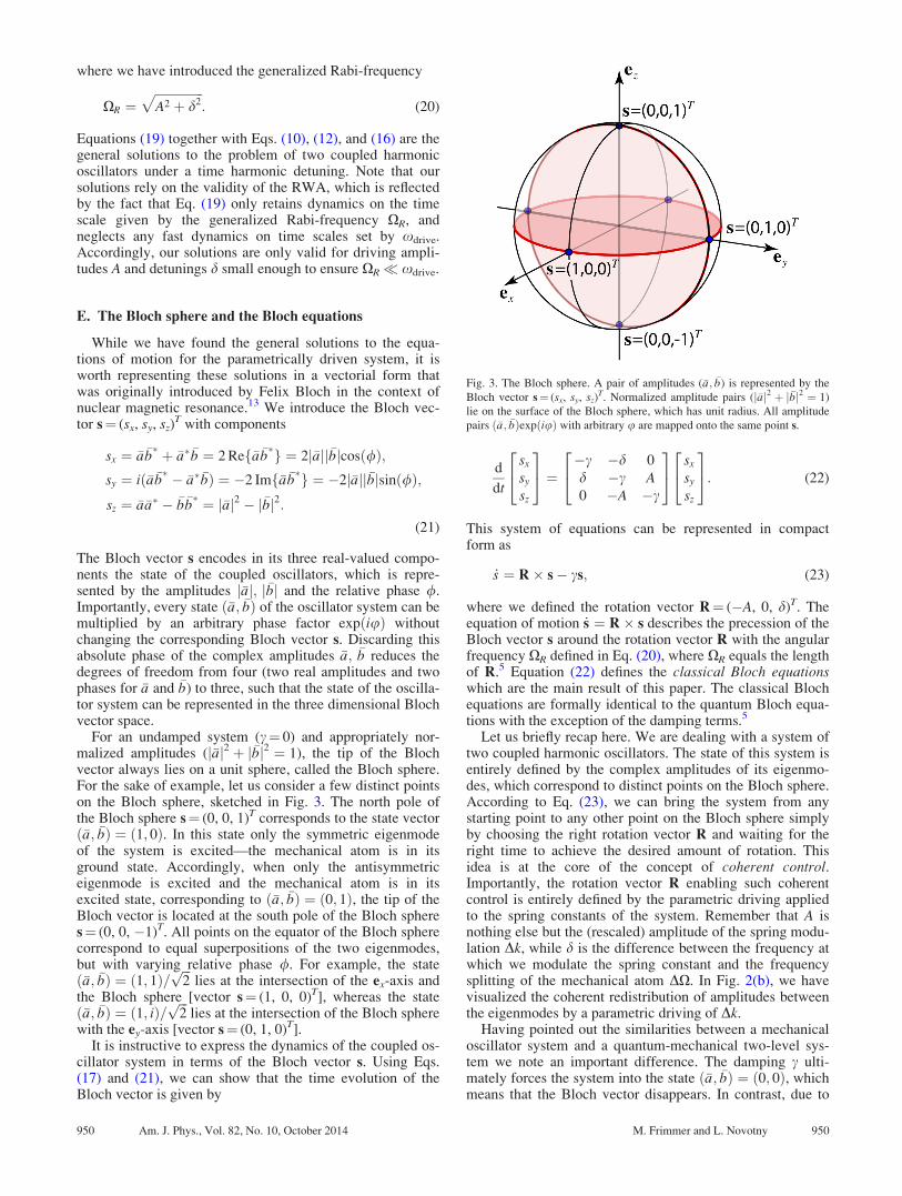
While we have found the general solutions to the equa-tions of motion for the parametrically driven system, it isworth representing these solutions in a vectorial form thatwas originally introduced by Felix Bloch in the context ofnuclear magnetic resonance.13 We introduce the Bloch vec-tor s¼ (sx, sy, sz)

T with components

sx ¼ �a �b� þ �a� �b ¼ 2 Ref�a �b

�g ¼ 2j�ajj�bjcosð/Þ;sy ¼ ið�a �b

� � �a� �bÞ ¼ �2 Imf�a �b�g ¼ �2j�ajj�bjsinð/Þ;

sz ¼ �a�a� � �b �b� ¼ j�aj2 � j�bj2:

(21)

The Bloch vector s encodes in its three real-valued compo-nents the state of the coupled oscillators, which is repre-sented by the amplitudes j�aj; j�bj and the relative phase /.Importantly, every state ð�a; �bÞ of the oscillator system can bemultiplied by an arbitrary phase factor expðiuÞ withoutchanging the corresponding Bloch vector s. Discarding thisabsolute phase of the complex amplitudes �a; �b reduces thedegrees of freedom from four (two real amplitudes and twophases for �a and �b) to three, such that the state of the oscilla-tor system can be represented in the three dimensional Blochvector space.

For an undamped system (c¼ 0) and appropriately nor-malized amplitudes (j�aj2 þ j�bj2 ¼ 1), the tip of the Blochvector always lies on a unit sphere, called the Bloch sphere.For the sake of example, let us consider a few distinct pointson the Bloch sphere, sketched in Fig. 3. The north pole ofthe Bloch sphere s¼ (0, 0, 1)T corresponds to the state vectorð�a; �bÞ ¼ ð1; 0Þ. In this state only the symmetric eigenmodeof the system is excited—the mechanical atom is in itsground state. Accordingly, when only the antisymmetriceigenmode is excited and the mechanical atom is in itsexcited state, corresponding to ð�a; �bÞ ¼ ð0; 1Þ, the tip of theBloch vector is located at the south pole of the Bloch spheres¼ (0, 0, �1)T. All points on the equator of the Bloch spherecorrespond to equal superpositions of the two eigenmodes,but with varying relative phase /. For example, the stateð�a; �bÞ ¼ ð1; 1Þ=

ffiffiffi2p

lies at the intersection of the ex-axis andthe Bloch sphere [vector s¼ (1, 0, 0)T], whereas the stateð�a; �bÞ ¼ ð1; iÞ=

ffiffiffi2p

lies at the intersection of the Bloch spherewith the ey-axis [vector s¼ (0, 1, 0)T].

It is instructive to express the dynamics of the coupled os-cillator system in terms of the Bloch vector s. Using Eqs.(17) and (21), we can show that the time evolution of theBloch vector is given by

d

dt

sx

sy

sz

24

35 ¼ �c �d 0

d �c A0 �A �c

24

35 sx

sy

sz

24

35: (22)

This system of equations can be represented in compactform as

_s ¼ R� s� cs; (23)

where we defined the rotation vector R¼ (�A, 0, d)T. Theequation of motion _s ¼ R� s describes the precession of theBloch vector s around the rotation vector R with the angularfrequency XR defined in Eq. (20), where XR equals the lengthof R.5 Equation (22) defines the classical Bloch equationswhich are the main result of this paper. The classical Blochequations are formally identical to the quantum Bloch equa-tions with the exception of the damping terms.5

Let us briefly recap here. We are dealing with a system oftwo coupled harmonic oscillators. The state of this system isentirely defined by the complex amplitudes of its eigenmo-des, which correspond to distinct points on the Bloch sphere.According to Eq. (23), we can bring the system from anystarting point to any other point on the Bloch sphere simplyby choosing the right rotation vector R and waiting for theright time to achieve the desired amount of rotation. Thisidea is at the core of the concept of coherent control.Importantly, the rotation vector R enabling such coherentcontrol is entirely defined by the parametric driving appliedto the spring constants of the system. Remember that A isnothing else but the (rescaled) amplitude of the spring modu-lation Dk, while d is the difference between the frequency atwhich we modulate the spring constant and the frequencysplitting of the mechanical atom DX. In Fig. 2(b), we havevisualized the coherent redistribution of amplitudes betweenthe eigenmodes by a parametric driving of Dk.

Having pointed out the similarities between a mechanicaloscillator system and a quantum-mechanical two-level sys-tem we note an important difference. The damping c ulti-mately forces the system into the state ð�a; �bÞ ¼ ð0; 0Þ, whichmeans that the Bloch vector disappears. In contrast, due to

Fig. 3. The Bloch sphere. A pair of amplitudes (�a; �b) is represented by the

Bloch vector s¼ (sx, sy, sz)T. Normalized amplitude pairs (j�aj2 þ j�bj2 ¼ 1)

lie on the surface of the Bloch sphere, which has unit radius. All amplitude

pairs ð�a; �bÞexpðiuÞ with arbitrary u are mapped onto the same point s.

950 Am. J. Phys., Vol. 82, No. 10, October 2014 M. Frimmer and L. Novotny 950

spontaneous emission, a quantum two-level system willalways end up in its ground state after a long time. Clearly,while the concept of coherent control can be applied toentirely classical systems, spontaneous emission is a processthat is genuinely quantum mechanical in nature and cannotbe recovered in a system governed by classical mechanics.It must be emphasized that spontaneous emission requires afully quantized theory and cannot be derived by semi-classical quantum mechanics. Even Bloch added the decayconstants semi-phenomenologically in his treatment ofnuclear spins.5 In quantum-mechanical systems, one com-monly distinguishes two decay rates. The first—the longitu-dinal decay rate c1¼ 1/T1—describes the decay of theinversion sz, while the second—the transverse decay ratec2¼ 1/T2—governs the decay of the components sx and sy ofthe Bloch vector. For the mechanical oscillator system, wefind c1¼ c2¼ c, which explains the recent experimental find-ing by Faust et al. in a micromechanical oscillator system.11

Finally, we stress that the analogy between a pair of coupledmechanical oscillators and a quantum two-level system relieson the SVEA and accordingly breaks down whenever theamplitudes �a; �b change on a time scale comparable to thecarrier frequency X0.

III. OPERATIONS ON THE BLOCH SPHERE

We have seen that by parametrically modulating thedetuning of the coupled oscillators we can control the trajec-tory of the Bloch vector on the Bloch sphere at will. Threeprotocols for Bloch vector manipulation have proven partic-ularly useful in the field of coherent control, leading to phe-nomena called Rabi oscillations, Ramsey fringes, and Hahnecho. We will now briefly discuss these phenomena.

A. Rabi oscillations

In 1937, Rabi studied the dynamics of a spin in a staticmagnetic field that is modulated by a radio-frequency fieldand he found that the spin vector periodically oscillatesbetween parallel and anti-parallel directions with respect tothe static magnetic field.14 These oscillations are referred toas Rabi oscillations, or Rabi flopping. The mechanical atomreproduces the basic physics of this Rabi flopping.

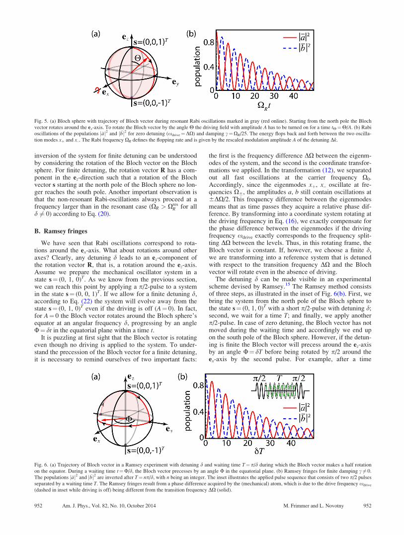
Let us neglect damping for the moment (c¼ 0) andassume a resonant (d¼ 0) parametric driving Dk /A cosðDX tÞ to our system, such that the Bloch vector, start-ing at the north pole s¼ (0, 0, 1)T, rotates around the axisR¼�Aex at a frequency XR¼A according to Eq. (23). Aftera time tp¼p/A the Bloch vector will have rotated to thesouth pole s¼ (0, 0, �1)T. This means that the symmetriceigenmode now has zero amplitude while the antisymmetriceigenmode has unit amplitude: ð�a; �bÞ ¼ ð0; 1Þ. Obviously,parametric driving for a time tp (called a p-pulse) inverts oursystem. Accordingly, after parametrically driving the systemfor a time t2p¼ 2p/A it has returned to its initial state at thenorth pole of the Bloch sphere.

We have plotted the populations of the eigenmodes forthree different pulse durations in Fig. 4. In general, for aH-pulse the parametric driving with amplitude A is turnedon for a time tH¼H/A. Remember that the driving signaloscillates at a frequency xdrive according to Eq. (15) andtherefore undergoes many oscillations during the pulse.Importantly, within the validity of the RWA, we can makeevery pulse arbitrarily short by applying a driving signal

with large amplitude A. For a continuous parametric driving,starting at s¼ (0, 0, 1)T, the system is oscillating between itstwo eigenmodes at the resonant Rabi-frequency XR¼A. Wecan explicitly convince ourselves that the picture of theBloch sphere yields the correct result by considering thetime evolution of the population of the eigenmodes, given byj�aj2 and j�bj2 in Eq. (19). For ð�a0; �b0Þ ¼ ð1; 0Þ, we obtain

j�aðtÞj2 ¼ cos2 XRt

2

� �e�ct

j�bðtÞj2 ¼ sin2 XRt

2

� �e�ct:

(24)

We plot the trajectory of the Bloch vector for a resonantlydriven system in Fig. 5(a) and the populations j�aj2 and j�bj2 inFig. 5(b). Indeed, for zero damping (c¼ 0) the energy oscil-lates back and forth between the two eigenmodes of the sys-tem at a frequency XR. However, a finite damping c makesthe population of both eigenmodes die out with progressingtime and the length of the Bloch vector is no longer con-served. For finite detuning (d 6¼ 0), we find that even withoutdamping the population inversion is reduced and no longerreaches a value of one. The population of the antisymmetriceigenmode reaches a maximum value of j�bðtpÞj2 ¼ A2=X2

R.The fact that the Rabi oscillations do not lead to a complete

Fig. 4. Controlling the dynamics of coupled oscillators with pulses of differ-

ent duration and amplitude. (a) Starting in the ground state ð�a; �bÞ ¼ ð1; 0Þ, a

p/2-pulse leaves both modes equally excited; (b) A p-pulse transfers the

energy of xþ to x–; and (c) a 2p pulse brings the system back to where it

started. In all cases we assumed no damping (c¼ 0) and no detuning (d¼ 0).

951 Am. J. Phys., Vol. 82, No. 10, October 2014 M. Frimmer and L. Novotny 951

inversion of the system for finite detuning can be understoodby considering the rotation of the Bloch vector on the Blochsphere. For finite detuning, the rotation vector R has a com-ponent in the ez-direction such that a rotation of the Blochvector s starting at the north pole of the Bloch sphere no lon-ger reaches the south pole. Another important observation isthat the non-resonant Rabi-oscillations always proceed at afrequency larger than in the resonant case (XR > Xres

R for alld 6¼ 0) according to Eq. (20).

B. Ramsey fringes

We have seen that Rabi oscillations correspond to rota-tions around the ex-axis. What about rotations around otheraxes? Clearly, any detuning d leads to an ez-component ofthe rotation vector R, that is, a rotation around the ez-axis.Assume we prepare the mechanical oscillator system in astate s¼ (0, 1, 0)T. As we know from the previous section,we can reach this point by applying a p/2-pulse to a systemin the state s¼ (0, 0, 1)T. If we allow for a finite detuning d,according to Eq. (22) the system will evolve away from thestate s¼ (0, 1, 0)T even if the driving is off (A¼ 0). In fact,for A¼ 0 the Bloch vector rotates around the Bloch sphere’sequator at an angular frequency d, progressing by an angleU¼ dt in the equatorial plane within a time t.

It is puzzling at first sight that the Bloch vector is rotatingeven though no driving is applied to the system. To under-stand the precession of the Bloch vector for a finite detuning,it is necessary to remind ourselves of two important facts:

the first is the frequency difference DX between the eigenm-odes of the system, and the second is the coordinate transfor-mations we applied. In the transformation (12), we separatedout all fast oscillations at the carrier frequency X0.Accordingly, since the eigenmodes xþ, x– oscillate at fre-quencies X6, the amplitudes a, b still contain oscillations at6DX/2. This frequency difference between the eigenmodesmeans that as time passes they acquire a relative phase dif-ference. By transforming into a coordinate system rotating atthe driving frequency in Eq. (16), we exactly compensate forthe phase difference between the eigenmodes if the drivingfrequency xdrive exactly corresponds to the frequency split-ting DX between the levels. Thus, in this rotating frame, theBloch vector is constant. If, however, we choose a finite d,we are transforming into a reference system that is detunedwith respect to the transition frequency DX and the Blochvector will rotate even in the absence of driving.

The detuning d can be made visible in an experimentalscheme devised by Ramsey.15 The Ramsey method consistsof three steps, as illustrated in the inset of Fig. 6(b). First, webring the system from the north pole of the Bloch sphere tothe state s¼ (0, 1, 0)T with a short p/2-pulse with detuning d;second, we wait for a time T; and finally, we apply anotherp/2-pulse. In case of zero detuning, the Bloch vector has notmoved during the waiting time and accordingly we end upon the south pole of the Bloch sphere. However, if the detun-ing is finite the Bloch vector will precess around the ez-axisby an angle U¼ dT before being rotated by p/2 around theex-axis by the second pulse. For example, after a time

Fig. 5. (a) Bloch sphere with trajectory of Bloch vector during resonant Rabi oscillations marked in gray (red online). Starting from the north pole the Bloch

vector rotates around the ex-axis. To rotate the Bloch vector by the angle H the driving field with amplitude A has to be turned on for a time tH¼H/A. (b) Rabi

oscillations of the populations j�aj2 and j�bj2 for zero detuning (xdrive¼DX) and damping c¼XR/25. The energy flops back and forth between the two oscilla-

tion modes xþ and x–. The Rabi frequency XR defines the flopping rate and is given by the rescaled modulation amplitude A of the detuning Dk.

Fig. 6. (a) Trajectory of Bloch vector in a Ramsey experiment with detuning d and waiting time T¼p/d during which the Bloch vector makes a half rotation

on the equator. During a waiting time t¼U/d, the Bloch vector precesses by an angle U in the equatorial plane. (b) Ramsey fringes for finite damping c 6¼ 0.

The populations j�aj2 and j�bj2 are inverted after T¼ np/d, with n being an integer. The inset illustrates the applied pulse sequence that consists of two p/2 pulses

separated by a waiting time T. The Ramsey fringes result from a phase difference acquired by the (mechanical) atom, which is due to the drive frequency xdrive

(dashed in inset while driving is off) being different from the transition frequency DX (solid).

952 Am. J. Phys., Vol. 82, No. 10, October 2014 M. Frimmer and L. Novotny 952

T¼ p/d the Bloch vector will have rotated to the points¼ (0, �1, 0)T such that the second p/2-pulse will bring thesystem back to the north pole s¼ (0, 0, 1)T, as plotted inFig. 6(a). If we measure the populations jaj2 and jbj2 afterthe second p/2-pulse we find the characteristic Ramseyfringes, plotted in Fig. 6(b), where we also included a finitedamping rate c that leads to an exponential decay of bothpopulations.

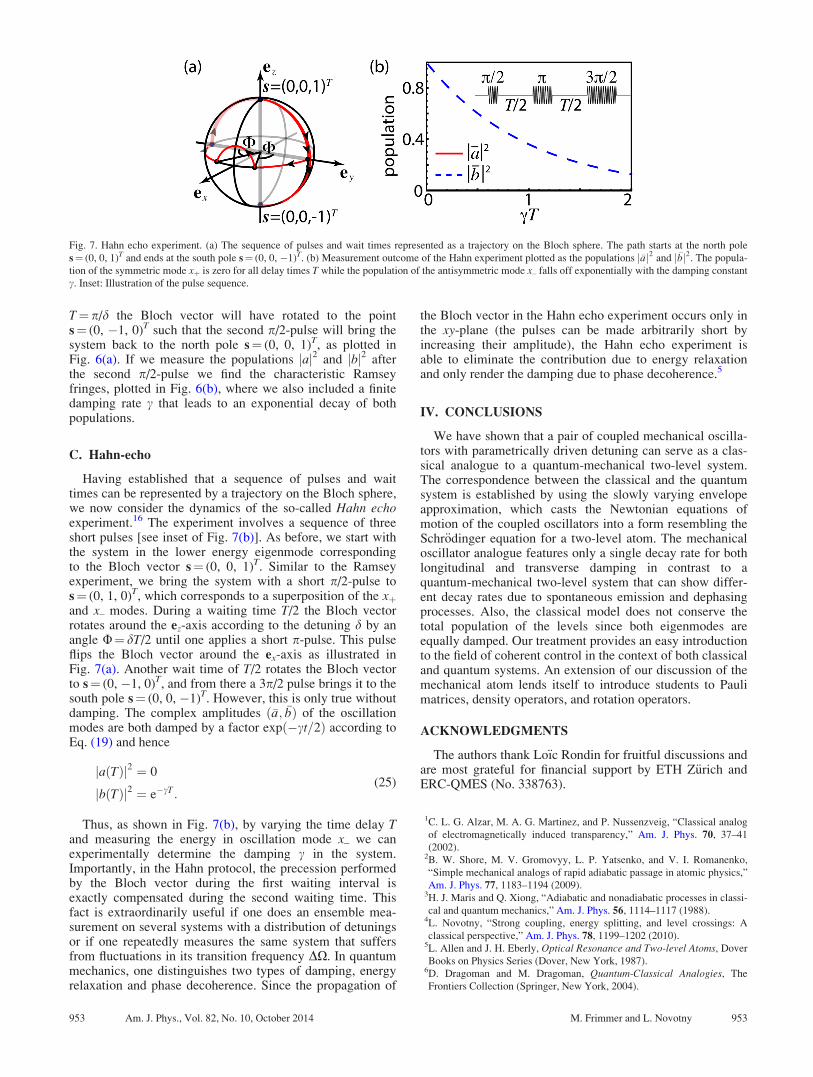
C. Hahn-echo

Having established that a sequence of pulses and waittimes can be represented by a trajectory on the Bloch sphere,we now consider the dynamics of the so-called Hahn echoexperiment.16 The experiment involves a sequence of threeshort pulses [see inset of Fig. 7(b)]. As before, we start withthe system in the lower energy eigenmode correspondingto the Bloch vector s¼ (0, 0, 1)T. Similar to the Ramseyexperiment, we bring the system with a short p/2-pulse tos¼ (0, 1, 0)T, which corresponds to a superposition of the xþand x– modes. During a waiting time T/2 the Bloch vectorrotates around the ez-axis according to the detuning d by anangle U¼ dT/2 until one applies a short p-pulse. This pulseflips the Bloch vector around the ex-axis as illustrated inFig. 7(a). Another wait time of T/2 rotates the Bloch vectorto s¼ (0, �1, 0)T, and from there a 3p/2 pulse brings it to thesouth pole s¼ (0, 0, �1)T. However, this is only true withoutdamping. The complex amplitudes ð�a; �bÞ of the oscillationmodes are both damped by a factor expð�ct=2Þ according toEq. (19) and hence

jaðTÞj2 ¼ 0

jbðTÞj2 ¼ e�cT :(25)

Thus, as shown in Fig. 7(b), by varying the time delay Tand measuring the energy in oscillation mode x– we canexperimentally determine the damping c in the system.Importantly, in the Hahn protocol, the precession performedby the Bloch vector during the first waiting interval isexactly compensated during the second waiting time. Thisfact is extraordinarily useful if one does an ensemble mea-surement on several systems with a distribution of detuningsor if one repeatedly measures the same system that suffersfrom fluctuations in its transition frequency DX. In quantummechanics, one distinguishes two types of damping, energyrelaxation and phase decoherence. Since the propagation of

the Bloch vector in the Hahn echo experiment occurs only inthe xy-plane (the pulses can be made arbitrarily short byincreasing their amplitude), the Hahn echo experiment isable to eliminate the contribution due to energy relaxationand only render the damping due to phase decoherence.5

IV. CONCLUSIONS

We have shown that a pair of coupled mechanical oscilla-tors with parametrically driven detuning can serve as a clas-sical analogue to a quantum-mechanical two-level system.The correspondence between the classical and the quantumsystem is established by using the slowly varying envelopeapproximation, which casts the Newtonian equations ofmotion of the coupled oscillators into a form resembling theSchr€odinger equation for a two-level atom. The mechanicaloscillator analogue features only a single decay rate for bothlongitudinal and transverse damping in contrast to aquantum-mechanical two-level system that can show differ-ent decay rates due to spontaneous emission and dephasingprocesses. Also, the classical model does not conserve thetotal population of the levels since both eigenmodes areequally damped. Our treatment provides an easy introductionto the field of coherent control in the context of both classicaland quantum systems. An extension of our discussion of themechanical atom lends itself to introduce students to Paulimatrices, density operators, and rotation operators.

ACKNOWLEDGMENTS

The authors thank Lo€ıc Rondin for fruitful discussions andare most grateful for financial support by ETH Z€urich andERC-QMES (No. 338763).

1C. L. G. Alzar, M. A. G. Martinez, and P. Nussenzveig, “Classical analog

of electromagnetically induced transparency,” Am. J. Phys. 70, 37–41

(2002).2B. W. Shore, M. V. Gromovyy, L. P. Yatsenko, and V. I. Romanenko,

“Simple mechanical analogs of rapid adiabatic passage in atomic physics,”

Am. J. Phys. 77, 1183–1194 (2009).3H. J. Maris and Q. Xiong, “Adiabatic and nonadiabatic processes in classi-

cal and quantum mechanics,” Am. J. Phys. 56, 1114–1117 (1988).4L. Novotny, “Strong coupling, energy splitting, and level crossings: A

classical perspective,” Am. J. Phys. 78, 1199–1202 (2010).5L. Allen and J. H. Eberly, Optical Resonance and Two-level Atoms, Dover

Books on Physics Series (Dover, New York, 1987).6D. Dragoman and M. Dragoman, Quantum-Classical Analogies, The

Frontiers Collection (Springer, New York, 2004).

Fig. 7. Hahn echo experiment. (a) The sequence of pulses and wait times represented as a trajectory on the Bloch sphere. The path starts at the north pole

s¼ (0, 0, 1)T and ends at the south pole s¼ (0, 0, �1)T. (b) Measurement outcome of the Hahn experiment plotted as the populations j�aj2 and j�bj2. The popula-

tion of the symmetric mode xþ is zero for all delay times T while the population of the antisymmetric mode x– falls off exponentially with the damping constant

c. Inset: Illustration of the pulse sequence.

953 Am. J. Phys., Vol. 82, No. 10, October 2014 M. Frimmer and L. Novotny 953

7M. E. Tobar and D. G. Blair, “A generalized equivalent circuit applied to a

tunable sapphire-loaded superconducting cavity,” IEEE Trans. Microw.

Theory Tech. 39, 1582–1594 (1991).8R. J. C. Spreeuw, N. J. van Druten, M. W. Beijersbergen, E. R. Eliel, and

J. P. Woerdman, “Classical realization of a strongly driven two-level sys-

tem,” Phys. Rev. Lett. 65, 2642–2645 (1990).9D. Bouwmeester, N. H. Dekker, F. E. v. Dorsselaer, C. A. Schrama, P. M.

Visser, and J. P. Woerdman, “Observation of Landau-Zener dynamics in

classical optical systems,” Phys. Rev. A 51, 646–654 (1995).10H. Okamoto, A. Gourgout, C.-Y. Chang, K. Onomitsu, I. Mahboob, E. Y.

Chang, and H. Yamaguchi, “Coherent phonon manipulation in coupled

mechanical resonators,” Nature Phys. 9, 480–484 (2013).

11T. Faust, J. Rieger, M. J. Seitner, J. P. Kotthaus, and E. M. Weig,

“Coherent control of a classical nanomechanical two-level system,”

Nature Phys. 9, 485–488 (2013).12M. Frimmer and A. F. Koenderink, “Superemitters in hybrid photonic sys-

tems: A simple lumping rule for the local density of optical states and its

breakdown at the unitary limit,” Phys. Rev. B 86, 235428-1–6 (2012).13F. Bloch, “Nuclear induction,” Phys. Rev. 70, 460–474 (1946).14I. I. Rabi, “Space quantization in a gyrating magnetic field,” Phys. Rev.

51, 652–654 (1937).15N. F. Ramsey, “A molecular beam resonance method with separated oscil-

lating fields,” Phys. Rev. 78, 695–699 (1950).16E. L. Hahn, “Spin echoes,” Phys. Rev. 80, 580–594 (1950).

954 Am. J. Phys., Vol. 82, No. 10, October 2014 M. Frimmer and L. Novotny 954