1

The Characteristics of Stock Market Volatility

By Daniel R Wessels

June 2006

Available at: www.indexinvestor.co.za

1. Introduction

Stock market volatility is synonymous with the uncertainty how macro-

economic events and trends will affect the future profitability (dividends, cash

flows) of listed companies and hence their market valuations. Typical

examples of such variables in the current environment are: geo-political

tensions, energy prices, inflation expectations, interest rate policies and the

stability of exchange rates. But then again, these uncertainties in some form

or another are always present; yet we find that stock market volatility is some

times much higher than in other periods.

Many research studies, such as Schwert (1989)1, have explained the variance

of stock market volatility with the time-varying volatility of a variety of

economic variables. For example, changes in inflation, money growth,

industrial production and other measures of economic activity are related to

changes in stock market volatility. Furthermore, volatility increases with the

financial leverage (debt) of companies. In addition, volatility is correlated with

interest rate movements and increases during economic recessions.

Stock markets in general have treated investors well over the past couple of

years with no major setbacks (until the beginning of May 2006). A prominent

feature has been the absence of volatility on stock markets and in general

markets followed one direction only, namely upwards. However, during the

year to date (May 2006) volatility once again has come to the fore as more

investors were piling into the investment markets (daily trade volumes of R8-

10bn) and stock prices soared to record levels2.

2

My main objective with this study is to analyse the typical characteristics of

stock market volatility on our local bourse (JSE). In this paper I endeavour to

answer questions such as: How did stock market volatility behave in the past?

Are there any identifiable patterns? Is there any meaningful link between

volatility and returns? How could one use this information to develop some

insight how to manage future volatility?

Monthly stock market data from 1960 until March 2006 (more than 46 years)

were used in this analysis. First, I provide some general background on the

meaning and implications of the volatility concept for investors. Second, I

analyse the typical characteristics of stock market volatility – its distribution,

movement patterns and duration intervals. Finally, I investigate the general

relationship between volatility and stock market returns with specific focus on

the correlation between changes in volatility and investment returns.

2. The Concept of Volatility: Back to Basics

Most investors perceive investment risk primarily as the risk of losing capital,

but it may also include the risk of not achieving a certain minimum return. In

short, investment risk can be defined as the possibility of being disenchanted

with your investment plan in not meeting your investment objectives.

Understandably, it is immensely difficult to develop a universal accepted

definition of investment risk since investors apply different time frames to the

outcome of their investing efforts. For example, some investors do not want

any capital losses over any period; another group might tolerate some short-

term losses in the hope of doing well in the long run, while others realise that

exceptional gains are not likely without exposing oneself to some real risk.

In order to gauge this likelihood of “disappointment”, the professional

investment industry uses a common indicator, namely the volatility of

investment returns. The volatility of stock market investments can be defined

3

as the dispersion of investment returns below and above the mean, otherwise

known as the standard deviation of returns.

The concept of volatility is widely used in the investment industry. Typically,

the allocation of investment strategies and fund selections to an investment

plan are based on their respective volatilities and whether it fits the risk profile

of the prospective investor. Therefore, it is important for investors to

understand the limitations and uses of volatility as a barometer of investment

risk.

First, it is important to understand how volatility is estimated. Typically, the

volatility of investments spanning over different intervals is standardised, for

example annualised volatility, to compare the riskiness of investment

portfolios. The following annualization rule applies:

Standard deviation over an interval x Square root of the number of intervals

per annum

For example, if the standard deviation measured on a weekly basis is equal to

2.5% and one wants to express the deviation on an annual basis, the

following formula will apply: 2.5% x SQRT(52) = 18%.

Note, it is not merely volatility on a weekly basis times the number of weeks in

a year, because such practice would have led to a gross overestimation of

volatility. In essence, the volatility of stock prices exhibits a mean-reverting

pattern.

Table 1 illustrates the various annualised rates over different measurement

periods.

4

Table 1: Converting different volatility measures to a standard basis

Measured Volatility Annualised Volatility

Std Deviation (daily) 1.2% 19.0%

Std Deviation (weekly) 2.5% 18.0%

Std Deviation (monthly) 5.5% 19.1%

Std Deviation (annually) 18.0%

Second, and in accordance with the first principle illustrated above, the

passing of time reduces volatility.

Consider the following two examples, a five-year investment and a ten-year

investment, shown in table 2 below:

Table 2: The passing of time reduces volatility

Period Capital Value Annual Return

Year 0 100

Year 1

115 15.0%

Year 2

106 -8.0%

Year 3

129 22.0%

Year 4

154 19.0%

Year 5

174 13.0%

Std Deviation 11.8%

Average Return 12.2%

Geometric return 11.7%

5

Table 2 (continued…)

Period Capital Value Annual Return

Year 0 100

Year 1

115 15.0%

Year 2

106 -8.0%

Year 3

129 22.0%

Year 4

154 19.0%

Year 5

174 13.0%

Year 6

200 15.0%

Year 7

184 -8.0%

Year 8

224 22.0%

Year 9

267 19.0%

Year 10

301 13.0%

Std Deviation 11.1%

Average Return 12.2%

Geometric return 11.7%

In the above example both investments yielded the same return; in fact the

five-year investment is identical to the ten-year investment, except for the

term. Note that the standard deviation in the latter is lower than in the former

investment (11.1% versus 11.8%).

From table 2 two other important inferences are made, first the average return

is higher than the geometric or annualised return and second, if the ten-year

investment is identical to the five-year investment, then one would have

expected the capital value after ten years to be exactly double the capital

value after five years (174 x 2 = 348), but it is not!

A third principle is hereby installed. Time reduces volatility, but not the value

at risk. This phenomenon is explained by the degenerating effect of volatility

on returns which lead to actual returns (geometric or annualised) being lower

6

than the average return. This difference is compounded with the passing of

time and leads to lower returns than it would have been predicted otherwise

(as illustrated in table 2).

In general the following rule applies:

Degeneration of returns = average return minus 50% of portfolio variance

(standard deviation squared).

A fourth principle is that volatility measures both the upside and downside

deviations from the mean. Nobody would mind the upside (higher returns), but

definitely the downside. Thus, one can identify both “good” and “bad”

volatilities. Examples of such investments are depicted in table 3 below.

Table 3: Same volatilities, different outcomes

Period Capital Value Annual Return

Year 0 100

Year 1 95 -5.0%

Year 2 112 17.9%

Year 3 125 11.6%

Year 4 139 11.2%

Year 5 150 7.9%

Std Deviation 8.5%

Average Return 8.7%

Geometric return 8.4%

7

Table 3 (continued…)

Period Capital Value Annual Return

Year 0 100

Year 1

100 0.0%

Year 2

122 22.0%

Year 3

143 17.0%

Year 4

154 8.0%

Year 5

174 13.0%

Std Deviation 8.5%

Average Return 12.0%

Geometric return 11.7%

From table 3 it is obvious that volatility must never be seen in isolation.

Investment return is the flipside of investment risk and should always be the

criterion upon which your investment decision is based.

Furthermore, although we know that high volatility leads to the degeneration

of investment returns it does not mean that volatility altogether should be

avoided. In fact, low volatility investments (like cash) generally lead to low

returns. Therefore, we should seek volatility to have any chance of making

real gains. However, when we evaluate two similar risky investments one can

compare their volatilities and respective returns. In essence, we want to invest

in those investments or assets that yield the highest return per unit risk

(volatility).

8

3. The Characteristics of Stock Market Volatility

3.1 The Distribution of Stock Market Volatility

The standard deviations of the JSE All Share Index (ALSI) monthly returns

from January 1960 to the end of March 2006 (in total 543 periods) were

computed and presented on an annualised basis.

Figure 1 and table 4 display the frequency distribution and statistical

description of the annualised volatilities recorded over time.

Frequency Distribution

Annualised VolatilityJan1960 - March 2006

0

10

20

30

40

50

60

70

4%

8%

11

%

15

%

18

%

22

%

25

%

29

%

32

%

36

%

39

%

43

%

Range

Fre

qu

en

cy

Figure 1: A graphical presentation of the frequency distribution of annualised volatilities in the

monthly return of the JSE All Share Index

9

Table 4: A statistical description of annualised stock market volatility (monthly

ALSI returns)

Mean 20.04%

Standard Error 0.33%

Median 19.14%

Standard Deviation 7.76%

Kurtosis 0.61

Skewness 0.75

Minimum 4.3%

Maximum 44.7%

The distribution of the monthly volatilities is asymmetrical and positively

skewed, meaning the occurrence of large volatilities to the right of the mean

(20%) with a maximum observed annualised volatility of near 45%.

10

3.2 The Clustering of Volatility

An important characteristic of stock market volatility is the tendency of

clustering, in other words volatility tends to stay more or less the same for

some time before it moves to a new level.

Figure 2 illustrates the clustering effect of volatility by means of an

autocorrelation analysis, which found that a positive autocorrelation is

statistically significant in 33 out of 36 consecutive months. This indicates that

the volatility in the preceding months have a profound affect on the volatility in

the following month – the so-called momentum effect.

Autocorrelations for Annualised Volatility

(significant values colored red)

-1.0

-0.5

0.0

0.5

1.0

1 2 3 4 5 6 7 8 9 10 11 12 13 14 15 16 17 18 19 20 21 22 23 24 25 26 27 28 29 30 31 32 33 34 35 36

Lag

Figure 2: Autocorrelations for annualised volatility, significant values

coloured red (lag = 36 months)

11

3.3 Volatility Patterns

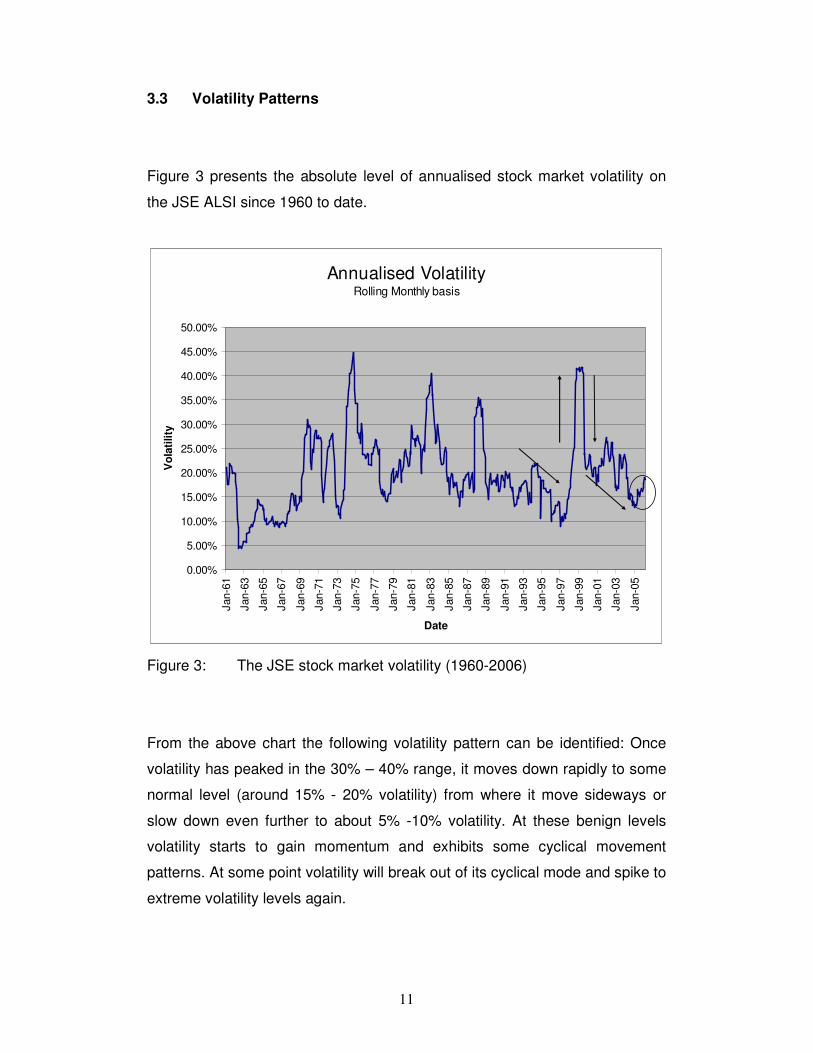
Figure 3 presents the absolute level of annualised stock market volatility on

the JSE ALSI since 1960 to date.

Annualised VolatilityRolling Monthly basis

0.00%

5.00%

10.00%

15.00%

20.00%

25.00%

30.00%

35.00%

40.00%

45.00%

50.00%

Jan-6

1

Jan-6

3

Jan-6

5

Jan-6

7

Jan-6

9

Jan-7

1

Jan-7

3

Jan-7

5

Jan-7

7

Jan-7

9

Jan-8

1

Jan-8

3

Jan-8

5

Jan-8

7

Jan-8

9

Jan-9

1

Jan-9

3

Jan-9

5

Jan-9

7

Jan-9

9

Jan-0

1

Jan-0

3

Jan-0

5Date

Vo

lati

lity

Figure 3: The JSE stock market volatility (1960-2006)

From the above chart the following volatility pattern can be identified: Once

volatility has peaked in the 30% – 40% range, it moves down rapidly to some

normal level (around 15% - 20% volatility) from where it move sideways or

slow down even further to about 5% -10% volatility. At these benign levels

volatility starts to gain momentum and exhibits some cyclical movement

patterns. At some point volatility will break out of its cyclical mode and spike to

extreme volatility levels again.

12

When studying the most recent period it is noticeable that volatility has started

to gain momentum and is heading upwards after reaching a low in the

beginning of 2005.

Although it is not within the realm of this study to investigate specifically why

volatility exhibited the pattern of tranquillity and violent eruptions in the past,

one generalisation can be put forward:

Changes in volatility reflect the changes in fundamental economic factors.

Greater volatility leads to a perception of greater risk to the present and future

value of assets. Increased volatility may simply reflect information and

expectations of changes in fundamental economic factors. If volatility either

exceeds or falls short of the level indicated by fundamental economic factors,

the result is mispricing, and as a consequence the misallocation of

resources3.

For example, during periods of low volatility investors on the aggregate are

prepared to pay too much for asset prices which lead to speculative bubbles

and eventually give rise to dramatic collapses in inflated asset prices.

3.4 Volatility Intervals

In the previous section we have seen that stock market volatility over time

exhibits a high-low pattern. In order to assess the average duration of volatility

at specific levels, the annualised volatilities since 1960 were categorized into

four quartiles. Table 5 displays the quartile ranges and the average duration

in each quartile.

13

Table 5: Quartile Ranking of Annualised Volatility (rolling monthly basis)

Annualised Volatility Range

Lower Volatility

Upper Volatility

Observations (months)

Average Duration (months)

Maximum Duration (months)

Q1 4.3% 14.8% 136 21 70

Q2 14.8% 19.1% 136 4 13

Q3 19.1% 24.1% 135 4 16

Q4 24.1% 44.7% 136 8 23

The high average duration found in the first quartile is skewed by a long-

lasting low volatility period from April 1962 to December 1967. When this

period is excluded, the average duration in the first quartile drops to 6 months

with a maximum duration period of 24 months.

Typically, it seems that volatility remains on average longer in the very low

and high volatility ranges (quartile one and four) than in the middle categories

(quartile two and three).

The rolling annualised volatility, expressed in quartiles, is graphically

displayed in figure 5.

Quartile Ranking of Volatility

1

2

3

4

Ja

n-6

1

Ja

n-6

3

Ja

n-6

5

Ja

n-6

7

Ja

n-6

9

Ja

n-7

1

Ja

n-7

3

Ja

n-7

5

Ja

n-7

7

Ja

n-7

9

Ja

n-8

1

Ja

n-8

3

Ja

n-8

5

Ja

n-8

7

Ja

n-8

9

Ja

n-9

1

Ja

n-9

3

Ja

n-9

5

Ja

n-9

7

Ja

n-9

9

Ja

n-0

1

Ja

n-0

3

Ja

n-0

5

Date

Qu

art

ile

Figure 5: Annualised volatility grouped in quartiles from 1960 to date

14

4. Volatility and Returns

High stock market volatilities imply the rapid changes in stock prices, and thus

returns, but do not explicitly imply whether stock market returns should be

positive or negative. Therefore, I endeavour to establish which return profile

can typically be expected for a certain level of stock market volatility.

Figure 6 portrays the annualised volatility plotted against the annual ALSI

returns on a monthly rolling basis. In some instances it can be seen that high

volatilities are accompanied by sharp stock market declines and vice versa,

but a more unambiguous analysis is required to make some meaningful

inferences.

Volatility and JSE ALSI ReturnsRolling monthly basis

0.00%

5.00%

10.00%

15.00%

20.00%

25.00%

30.00%

35.00%

40.00%

45.00%

50.00%

Jan-6

1

Jan-6

4

Jan-6

7

Jan-7

0

Jan-7

3

Jan-7

6

Jan-7

9

Jan-8

2

Jan-8

5

Jan-8

8

Jan-9

1

Jan-9

4

Jan-9

7

Jan-0

0

Jan-0

3

Jan-0

6

Period

An

nu

alised

Vo

lati

lity

-60.00%

-40.00%

-20.00%

0.00%

20.00%

40.00%

60.00%

80.00%

100.00%

120.00%

An

nu

al R

etu

rn

Annualised Return Annualised Volatility

Figure 6: Annualised volatility and stock market return: 1960 – 2006

15

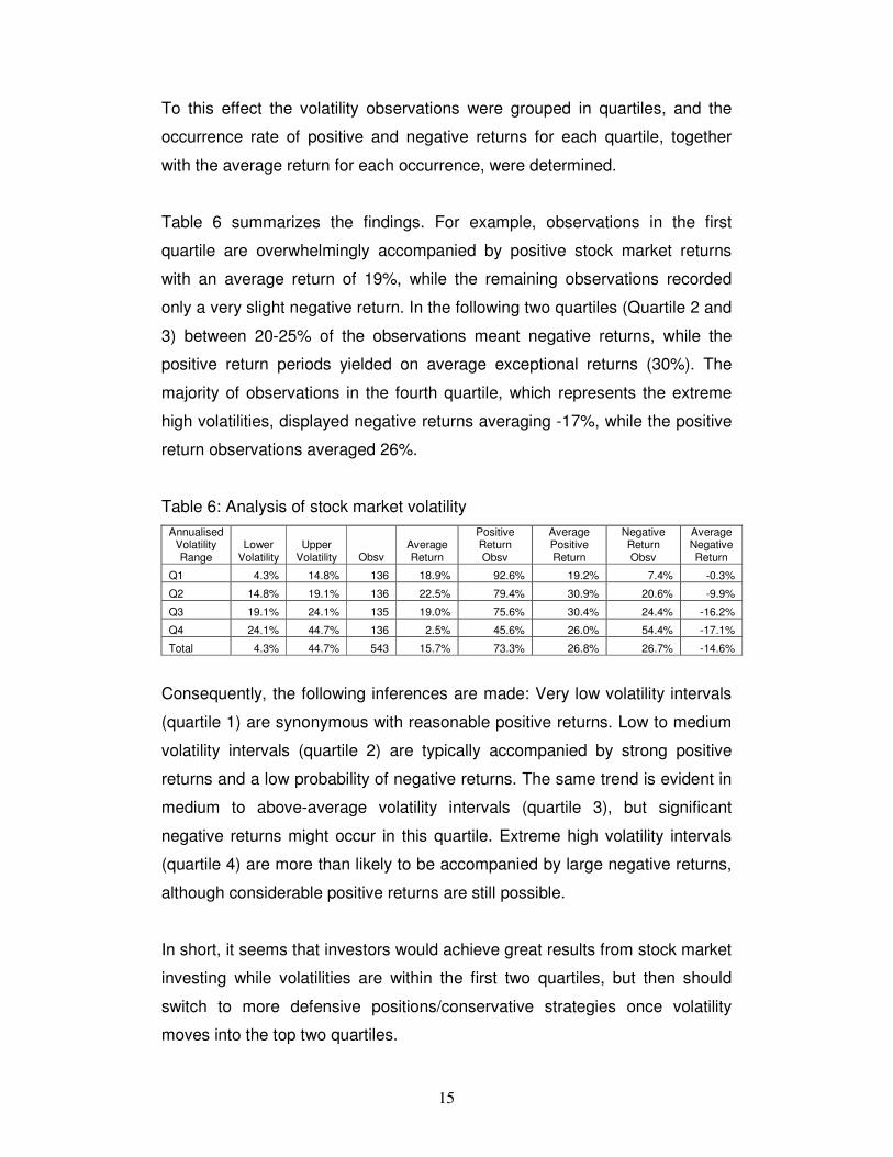
To this effect the volatility observations were grouped in quartiles, and the

occurrence rate of positive and negative returns for each quartile, together

with the average return for each occurrence, were determined.

Table 6 summarizes the findings. For example, observations in the first

quartile are overwhelmingly accompanied by positive stock market returns

with an average return of 19%, while the remaining observations recorded

only a very slight negative return. In the following two quartiles (Quartile 2 and

3) between 20-25% of the observations meant negative returns, while the

positive return periods yielded on average exceptional returns (30%). The

majority of observations in the fourth quartile, which represents the extreme

high volatilities, displayed negative returns averaging -17%, while the positive

return observations averaged 26%.

Table 6: Analysis of stock market volatility

Annualised Volatility Range

Lower Volatility

Upper Volatility Obsv

Average Return

Positive Return Obsv

Average Positive Return

Negative Return Obsv

Average Negative Return

Q1 4.3% 14.8% 136 18.9% 92.6% 19.2% 7.4% -0.3%

Q2 14.8% 19.1% 136 22.5% 79.4% 30.9% 20.6% -9.9%

Q3 19.1% 24.1% 135 19.0% 75.6% 30.4% 24.4% -16.2%

Q4 24.1% 44.7% 136 2.5% 45.6% 26.0% 54.4% -17.1%

Total 4.3% 44.7% 543 15.7% 73.3% 26.8% 26.7% -14.6%

Consequently, the following inferences are made: Very low volatility intervals

(quartile 1) are synonymous with reasonable positive returns. Low to medium

volatility intervals (quartile 2) are typically accompanied by strong positive

returns and a low probability of negative returns. The same trend is evident in

medium to above-average volatility intervals (quartile 3), but significant

negative returns might occur in this quartile. Extreme high volatility intervals

(quartile 4) are more than likely to be accompanied by large negative returns,

although considerable positive returns are still possible.

In short, it seems that investors would achieve great results from stock market

investing while volatilities are within the first two quartiles, but then should

switch to more defensive positions/conservative strategies once volatility

moves into the top two quartiles.

16

The validity of the above argument is reasonably confirmed when one

compares the historical stock market returns with its volatility since 1960 to

date (figure 7). Typically, sharp declines in annual returns very often occurred

when volatilities peaked (quartile 4), while periods of lower volatilities

(quartiles 1, 2 and 3) were accompanied by reasonable to exceptional stock

market returns.

Volatility and Returns

-60%

-40%

-20%

0%

20%

40%

60%

80%

100%

120%

Ja

n-6

1

Ja

n-6

3

Ja

n-6

5

Ja

n-6

7

Ja

n-6

9

Ja

n-7

1

Ja

n-7

3

Ja

n-7

5

Ja

n-7

7

Ja

n-7

9

Ja

n-8

1

Ja

n-8

3

Ja

n-8

5

Ja

n-8

7

Ja

n-8

9

Ja

n-9

1

Ja

n-9

3

Ja

n-9

5

Ja

n-9

7

Ja

n-9

9

Ja

n-0

1

Ja

n-0

3

Ja

n-0

5Date

An

nu

al R

etu

rn

1

2

3

4

Vo

lati

lity

Qu

art

ile

Figure 7: Stock market returns and volatility (quartiles): 1960 – 2006

17

5. Volatility Rate Changes

Thus far we have seen that periods of high volatilities are often associated

with negative returns, and lower volatility intervals with positive returns. But

this is not an infallible rule. Moreover, if volatility is currently at benign levels

and is moving gradually upwards, what does that implicate for stock market

returns? Alternatively, what if volatility increases/decreases rapidly from one

period to another?

Therefore, the relationship between stock market returns and the direction (up

or down) and velocity of volatility change from one period to another is

analysed in tables 7, 8 and 9 for different time intervals.

Table 7: The correlation between monthly changes in volatility and return

Volatility Change

M-o-M

Observations

(cumulative percentage) Correlation

0.00% 100% -0.27

0.50% 60% -0.29

1.00% 40% -0.33

1.50% 30% -0.37

2.00% 21% -0.43

2.50% 15% -0.48

3.00% 11% -0.48

3.50% 8% -0.51

4.00% 6% -0.57

4.50% 5% -0.63

5.00% 4% -0.63

5.50% 4% -0.66

6.00% 3% -0.72

6.50% 3% -0.70

7.00% 1% -0.85

18

Table 8: The correlation between quarterly changes in volatility and return

Volatility Change Q-t-Q

Observations (cumulative percentage) Correlation

0.00% 100% -0.25

0.50% 86% -0.26

1.00% 71% -0.27

1.50% 60% -0.28

2.00% 49% -0.29

2.50% 39% -0.31

3.00% 32% -0.32

3.50% 26% -0.34

4.00% 20% -0.38

4.50% 18% -0.40

5.00% 15% -0.42

5.50% 14% -0.41

6.00% 13% -0.45

6.50% 11% -0.48

7.00% 9% -0.55

7.50% 7% -0.54

8.00% 5% -0.55

8.50% 5% -0.54

9.00% 5% -0.66

9.50% 4% -0.69

10.00% 3% -0.69

Table 9: The correlation between yearly changes in volatility and return

Volatility Change Y-o-Y

Observations (cumulative percentage) Correlation

0.00% 100% -0.23

1.00% 88% -0.24

2.00% 77% -0.26

3.00% 66% -0.27

4.00% 54% -0.30

5.00% 47% -0.31

6.00% 37% -0.37

7.00% 33% -0.38

8.00% 29% -0.41

9.00% 26% -0.43

10.00% 24% -0.43

11.00% 22% -0.47

12.00% 19% -0.54

13.00% 16% -0.53

14.00% 15% -0.54

15.00% 13% -0.56

16.00% 10% -0.52

17.00% 8% -0.57

18.00% 6% -0.63

19.00% 6% -0.66

20.00% 5% -0.63

19

From the above tables: The majority of incremental changes (80-90%) are

weak to moderate, but this is not too surprising; we have seen that volatilities

tend to cluster around a certain level. In such instances, no statistically

significant relationship is found between the change in volatility and

investment returns.

However, when substantial changes in volatility do occur, a definite inverse

relationship with investment returns does hold. For example, a substantial rise

in volatility from one period to another is normally accompanied by large

negative returns. Alternatively, a sharp decline in volatility goes together with

considerable positive returns.

20

6. Conclusions

Stock market volatility tends to be sticky – meaning that the volatility level

over a certain period remains more or less stable until some material changes

in macro-economic variables are recognised, for example, increased

uncertainty about future interest rate policies. The uncertainty will cause

volatility to spike and a new pattern of volatility is established, which will

continue until more certainty about future monetary policies are installed. At

that stage volatility might calm down rapidly until it settles down at some

normalised level.

The above pattern is fairly predictable4 – although the underlying forces

driving volatility are not – and has some important implications for stock

market investors:

For example, in this study we found that investors on the aggregate should be

doing well while volatility is benign and at below-average levels. However,

some macro-economic shocks may cause volatility to spike, which normally

leads to sharp negative returns. Thereafter, the continuous uncertainty will

cause volatility to move within above-average and high volatility levels.

Positive returns at this stage are still very much a possibility, although large

negative returns can occur, especially when volatility reaches extreme levels.

Eventually, favourable macro-economic news will lead to a sharp reduction in

volatility, accompanied by strong positive returns, until volatility eases out at

an average or below-average level and the cycle is repeated.

At present (June 2006) stock market volatility has shot up with the

uncertainties surrounding future interest rate policies and we experienced the

consequential sharp sell-off (negative returns) in our market. Going forward, I

expect volatility to move in the third quartile range (above-average level) until

macro-economic conditions turn favourable again. Thus, one can expect

predominantly positive returns, but with some negative returns in between,

from the stock market in the forthcoming months. Overall, expect a moderate

to subdued stock market performance.

21

1 G.W.Schwert, 1989. “Why Does Stock Market Volatility Change Over Time?” The

Journal of Finance, 44(5), 1115-1153.

2 When I started with the project early May 2006 I was of the opinion that the stock

market volatility topic could soon be relevant for investors, yet little did I know that

merely two weeks later it was a very hot topic indeed as some dramatic down- and

upward movements in stock prices started to occur!

3 Karmakar, M. 2006. “Stock Market Volatility in the Long Run, 1961-2005”

Economic and Political Weekly, May 6, 1796-1802.

4 I do not necessarily consider my findings about volatility patterns to be a “sharp

predictive” tool, but rather a “blunt expectations” tool.