The CFD simulation of an axial ow fanAbstract The CFD simulation of an axial ow fan F.N. le Roux...
136
Transcript of The CFD simulation of an axial ow fanAbstract The CFD simulation of an axial ow fan F.N. le Roux...

The CFD simulation of an axial �ow fan
by
Frederick Nicolaas le Roux
Master of Science in Mechanical Engineering
Thesis presented in partial ful�lment of the requirements for
the degree of Master of Science in Mechanical Engineering at
Stellenbosch University
Department of Mechanical and Mechatronic Engineering,University of Stellenbosch,
Private Bag X1, Matieland 7602, South Africa.
Supervisor: Mr. S.J. van der SpuyCo-supervisor: Prof. T.W. von Backström
March 2010

Declaration
By submitting this thesis electronically, I declare that the entirety of the workcontained therein is my own, original work, that I am the owner of the copy-right thereof (unless to the extent explicitly otherwise stated) and that I havenot previously in its entirety or in part submitted it for obtaining any quali�-cation.
Signature: . . . . . . . . . . . . . . . . . . . . . . . . . . .F.N. le Roux
Date: . . . . . . . . . . . . . . . . . . . . . . . . . . . . . . .
Copyright © 2010 Stellenbosch UniversityAll rights reserved.
i

Abstract
The CFD simulation of an axial �ow fan
F.N. le Roux
Department of Mechanical and Mechatronic Engineering,University of Stellenbosch,
Private Bag X1, Matieland 7602, South Africa.
Thesis: MScEng (Mech)
March 2010
The purpose of this project is to investigate the method and accuracy of simu-lating axial �ow fans with three-dimensional axisymmetric CFD models. Twomodels are evaluated and compared with experimental fan data. Veri�cationdata is obtained from a prototype fan tested in a facility conforming to the BS848 standards. The �ow �eld over the blade surfaces is investigated furtherwith a visualization experiment comprising of a stroboscope and wool tufts.Good correlation is found at medium to high �ow rates and recommendationsare made for simulation at lower �ow rates as well as test guidelines at the fantest facility. The results and knowledge gained will be used to amend currentlyused actuator disc theory for axial �ow fan simulation.
Key words: CFD, NUMECA, axial �ow fan, �ow visualization
ii

Uittreksel
Die BVD simulasie van `n aksiaalwaaier
(�The CFD simulation of an axial �ow fan�)
F.N. le Roux
Departement Meganiese en Megatroniese Ingenieurswese,Universiteit van Stellenbosch,
Privaatsak X1, Matieland 7602, Suid Afrika.
Tesis: MScIng (Meg)
Maart 2010
Die doel van hierdie projek is om die metode en akkuraatheid om aksiaalvloei-waaiers met drie-dimensionele BVM modelle te simuleer, te ondersoek. Tweemodelle word geëvalueer en met eksperimentele waaiertoetse vergelyk. Veri-�kasie data is verkry vanaf `n prototipe waaier wat in `n fasiliteit getoets is enwat aan die BS 848 standaarde voldoen. Die vloeiveld oor die lemoppervlak-tes word ondersoek met `n visualisering eksperiment wat uit `n stroboskoop enwolletjies bestaan. Goeie korrelasie word gevind vir medium tot hoë massa-vloeie en aanbevelings word gemaak vir die simulasie by laer massavloeie metriglyne vir toetswerk in die toets-fasiliteit. Die resultate en kennis opgedoensal gebruik word in die verbetering van huidige aksieskyfteorie vir numerieseaksiaalvloeiwaaier simulasies.
Sleutelwoorde: BVM, NUMECA, aksiaalvloeiwaaier, vloei visualisering.
iii

Acknowledgements
I would like to express my sincere gratitude to the following people and organ-isations:
� My two supervisors for their continued support and guidance throughoutthe duration of the project. Thank you Mr. SJ van der Spuy for yourmotivation and encouragement in tiring times.
� Fluxion for their �nancial support.
� My family for continually pushing me and giving me the determinationto �nish.
� My friends for their motivation, in particular Andrew de Wet. Thankyou for joining me on this journey.
� And �nally my Lord the Saviour, without whom this and every achieve-ment in my life would not be possible.
iv

Dedications
This thesis is dedicated to my parents, for their perpetual love.
v

Contents
Declaration i
Abstract ii
Uittreksel iii
Acknowledgements iv
Dedications v
Contents vi
List of Figures ix
List of Tables xii
Nomenclature xiii
1 Introduction 1
2 Literature survey 6
2.1 Introduction . . . . . . . . . . . . . . . . . . . . . . . . . . . . . 62.1.1 Simulation of an axial �ow fan . . . . . . . . . . . . . . . 62.1.2 Experimental . . . . . . . . . . . . . . . . . . . . . . . . 10
2.2 Summary of main �ndings . . . . . . . . . . . . . . . . . . . . . 12
3 Numerical modelling 14
3.1 Introduction . . . . . . . . . . . . . . . . . . . . . . . . . . . . . 143.2 Fan blade data . . . . . . . . . . . . . . . . . . . . . . . . . . . 143.3 Computational domain . . . . . . . . . . . . . . . . . . . . . . . 16
3.3.1 AutoGrid� . . . . . . . . . . . . . . . . . . . . . . . . . 163.3.2 IGG� . . . . . . . . . . . . . . . . . . . . . . . . . . . . 183.3.3 Domain speci�cations . . . . . . . . . . . . . . . . . . . . 19
3.4 Computational parameters . . . . . . . . . . . . . . . . . . . . . 293.4.1 Fluid Model . . . . . . . . . . . . . . . . . . . . . . . . . 293.4.2 Flow Model . . . . . . . . . . . . . . . . . . . . . . . . . 30
vi

CONTENTS vii
3.4.3 Rotating Machinery . . . . . . . . . . . . . . . . . . . . . 303.4.4 Boundary Conditions . . . . . . . . . . . . . . . . . . . . 333.4.5 Numerical Model . . . . . . . . . . . . . . . . . . . . . . 343.4.6 Initial Solution . . . . . . . . . . . . . . . . . . . . . . . 383.4.7 Output . . . . . . . . . . . . . . . . . . . . . . . . . . . . 383.4.8 Computation Steering and Monitoring . . . . . . . . . . 38
3.5 Governing Equations . . . . . . . . . . . . . . . . . . . . . . . . 393.5.1 General Navier-Stokes Equations . . . . . . . . . . . . . 393.5.2 Time averaging of quantities . . . . . . . . . . . . . . . . 403.5.3 Treatment of turbulence in the equations . . . . . . . . . 413.5.4 Formulation in rotating frame for the relative velocity . . 413.5.5 Formulation in rotating frame for the absolute velocity . 42
4 Experimental evaluation 44
4.1 Introduction . . . . . . . . . . . . . . . . . . . . . . . . . . . . . 444.2 Fan Test Facility . . . . . . . . . . . . . . . . . . . . . . . . . . 444.3 Experimental setup parameters . . . . . . . . . . . . . . . . . . 45
4.3.1 Fan axis position . . . . . . . . . . . . . . . . . . . . . . 464.3.2 Blade angle . . . . . . . . . . . . . . . . . . . . . . . . . 464.3.3 Tip clearance . . . . . . . . . . . . . . . . . . . . . . . . 464.3.4 Root seals . . . . . . . . . . . . . . . . . . . . . . . . . . 47
4.4 Experiment . . . . . . . . . . . . . . . . . . . . . . . . . . . . . 474.5 Data Processing . . . . . . . . . . . . . . . . . . . . . . . . . . . 484.6 Results . . . . . . . . . . . . . . . . . . . . . . . . . . . . . . . . 48
4.6.1 Repeatability . . . . . . . . . . . . . . . . . . . . . . . . 484.6.2 Comparison with previous work . . . . . . . . . . . . . . 49
4.7 Conclusion . . . . . . . . . . . . . . . . . . . . . . . . . . . . . . 52
5 CFD validation with experimental data 54
5.1 Introduction . . . . . . . . . . . . . . . . . . . . . . . . . . . . . 545.2 Fan performance curve . . . . . . . . . . . . . . . . . . . . . . . 545.3 Transition . . . . . . . . . . . . . . . . . . . . . . . . . . . . . . 565.4 Investigation of streamline distribution . . . . . . . . . . . . . . 585.5 Flow pattern visualization . . . . . . . . . . . . . . . . . . . . . 60
6 Conclusion and recommendations 69
6.1 Motivation for study . . . . . . . . . . . . . . . . . . . . . . . . 696.2 Research �ndings . . . . . . . . . . . . . . . . . . . . . . . . . . 70
6.2.1 Experimental . . . . . . . . . . . . . . . . . . . . . . . . 706.2.2 Numerical Simulation . . . . . . . . . . . . . . . . . . . . 71
6.3 Recommendations for future research . . . . . . . . . . . . . . . 72
Appendices 75

CONTENTS viii
A Fan blade data for numerical simulation 76
B Sample calculations for experimental data 79
B.1 Sample Calculations . . . . . . . . . . . . . . . . . . . . . . . . 80
C Experimental Data 85
D Experimental Instrumentation 92
D.1 Ambient Conditions . . . . . . . . . . . . . . . . . . . . . . . . . 94D.2 Pressure . . . . . . . . . . . . . . . . . . . . . . . . . . . . . . . 94D.3 Torque . . . . . . . . . . . . . . . . . . . . . . . . . . . . . . . . 95D.4 Speed . . . . . . . . . . . . . . . . . . . . . . . . . . . . . . . . 95D.5 Bridge ampli�er . . . . . . . . . . . . . . . . . . . . . . . . . . . 95D.6 Blade angle setting jig . . . . . . . . . . . . . . . . . . . . . . . 95
E Calibration of instrumentation 98
E.1 Pressure Calibration . . . . . . . . . . . . . . . . . . . . . . . . 98E.2 Torque Calibration . . . . . . . . . . . . . . . . . . . . . . . . . 100E.3 Speed Calibration . . . . . . . . . . . . . . . . . . . . . . . . . . 103
F Fan performance characteristics 105
G Numerical Simulation Data 113
H Streamline distribution diagrams 115
List of References 119

List of Figures
1.1 The Matimba direct dry-cooled power plant (www.eskom.co.za). . . 21.2 Direct air-cooled condensing system with A-frame heat exchanger
con�guration. . . . . . . . . . . . . . . . . . . . . . . . . . . . . . . 3
2.1 ADM compared to experimental data (Van der Spuy et al. (2009)). 92.2 Main fan rotor dimensions and set-up, adapted from Meyer (1996). 122.3 Blade stagger angle and blade setting angle. . . . . . . . . . . . . . 13
3.1 Leading edge grid point distribution. . . . . . . . . . . . . . . . . . 163.2 O4H topology blocks and grid points, (AutoGrid� Manual, 2007a). 183.3 Azimuthal view of computational domain dimensions, Approach-1. . 203.4 Isometric grid view of computational domain, Approach-1. . . . . . 203.5 Azimuthal view of computational domain dimensions, Approach-2. . 213.6 Isometric grid view of computational domain, Approach-2. . . . . . 213.7 Isometric grid view of computational domain inlet section. . . . . . 223.8 Isometric grid view of computational domain inlet section solid
boundaries. . . . . . . . . . . . . . . . . . . . . . . . . . . . . . . . 233.9 A single blade generated in AutoGrid�. . . . . . . . . . . . . . . . . 243.10 y+
1 values for the blade section. . . . . . . . . . . . . . . . . . . . . 25(a) y+
1 range 1 to 10. . . . . . . . . . . . . . . . . . . . . . . . 25(b) y+
1 range 1 to 5. . . . . . . . . . . . . . . . . . . . . . . . . 25(c) y+
1 near tip gap. . . . . . . . . . . . . . . . . . . . . . . . . 253.11 Axisymetric nature of CFD model. . . . . . . . . . . . . . . . . . . 26
(a) 18
thaxisymmetric model, without repetition. . . . . . . . . 26
(b) 18
thaxisymmetric model, with repetition. . . . . . . . . . . 26
3.12 Averaged surfaces for obtaining outlet pressure. . . . . . . . . . . . 273.13 Isometric grid view of computational domain outlet section, Approach-
1. . . . . . . . . . . . . . . . . . . . . . . . . . . . . . . . . . . . . . 283.14 Isometric grid view of computational domain outlet section, Approach-
2. . . . . . . . . . . . . . . . . . . . . . . . . . . . . . . . . . . . . . 283.15 Static pressure distribution over the mixing plane approach rotor-
stator interface. . . . . . . . . . . . . . . . . . . . . . . . . . . . . . 313.16 Static pressure distribution over the frozen rotor rotor-stator inter-
face. . . . . . . . . . . . . . . . . . . . . . . . . . . . . . . . . . . . 32
ix

LIST OF FIGURES x
3.17 Mutigrid Strategy. . . . . . . . . . . . . . . . . . . . . . . . . . . . 363.18 Multigrid resolution for the blade hub. . . . . . . . . . . . . . . . . 36
(a) Finest mesh resolution, 000. . . . . . . . . . . . . . . . . . 36(b) Coarser mesh resolution, 111. . . . . . . . . . . . . . . . . 36(c) Coarsest mesh resolution, 222. . . . . . . . . . . . . . . . . 36
4.1 BS 848 Fan Test Facility, Stinnes (1998). . . . . . . . . . . . . . . . 454.2 Fan static pressure rise, repeatability. . . . . . . . . . . . . . . . . . 494.3 Fan power, repeatability. . . . . . . . . . . . . . . . . . . . . . . . . 494.4 Fan static e�ciency, repeatability. . . . . . . . . . . . . . . . . . . . 504.5 Fan static pressure rise, comparison with Stinnes (1998). . . . . . . 504.6 Fan power, comparison with Stinnes (1998). . . . . . . . . . . . . . 514.7 Fan static e�ciency, comparison with Stinnes (1998). . . . . . . . . 52
5.1 Fan static pressure rise, CFD veri�cation. . . . . . . . . . . . . . . 555.2 Fan power, CFD veri�cation. . . . . . . . . . . . . . . . . . . . . . 565.3 Fan static e�ciency, CFD veri�cation. . . . . . . . . . . . . . . . . 575.4 Streamline distribution, 16 m3/s, Approach-1, relative velocity so-
lution. . . . . . . . . . . . . . . . . . . . . . . . . . . . . . . . . . . 585.5 Streamline distribution, 16 m3/s, Approach-1, absolute velocity so-
lution. . . . . . . . . . . . . . . . . . . . . . . . . . . . . . . . . . . 595.6 Streamline distribution, 16 m3/s, Approach-2, absolute velocity so-
lution. . . . . . . . . . . . . . . . . . . . . . . . . . . . . . . . . . . 605.7 Streamline distribution close-up views for Approach-1 and Approach-
2. . . . . . . . . . . . . . . . . . . . . . . . . . . . . . . . . . . . . . 61(a) Streamline distribution, 16 m3/s, Approach-1, close-up. . . 61(b) Streamline distribution, 16 m3/s, Approach-2, close-up. . . 61
5.8 Streamline distribution, 8 m3/s, Approach-2, close-up view. . . . . . 615.9 Flow pattern visualization at 2 m3/s. . . . . . . . . . . . . . . . . . 65
(a) Experimental fan blade �ow pattern with throttle deviceclosed. . . . . . . . . . . . . . . . . . . . . . . . . . . . . . 65
(b) CFD fan blade �ow pattern at 2 m3/s (Approach-1). . . . 655.10 Flow pattern visualization at 10 m3/s. . . . . . . . . . . . . . . . . 66
(a) Experimental fan blade �ow pattern at 10 m3/s. . . . . . . 66(b) CFD fan blade �ow pattern at 10 m3/s (Approach-1). . . . 66(c) CFD fan blade �ow pattern at 10 m3/s (Approach-2). . . . 66
5.11 Flow pattern visualization at 16 m3/s. . . . . . . . . . . . . . . . . 67(a) Experimental fan blade �ow pattern at 16 m3/s. . . . . . . 67(b) CFD fan blade �ow pattern at 16 m3/s (Approach-1). . . . 67(c) CFD fan blade �ow pattern at 16 m3/s (Approach-2.) . . . 67
5.12 Flow pattern visualization at 20 m3/s. . . . . . . . . . . . . . . . . 68(a) Experimental fan blade �ow pattern with throttle device
fully open. . . . . . . . . . . . . . . . . . . . . . . . . . . . 68(b) CFD fan blade �ow pattern at 20 m3/s (Approach-1). . . . 68

LIST OF FIGURES xi
(c) CFD fan blade �ow pattern at 20 m3/s (Approach-2). . . . 68
A.1 Chord length and stagger angle distribution. . . . . . . . . . . . . . 76A.2 A plot of the GA(W)-2 and LS(1)-0413 pro�les. . . . . . . . . . . . 77
D.1 Schematic layout of experimental instrumentation. . . . . . . . . . 93D.2 Blade stagger angle setting jig. . . . . . . . . . . . . . . . . . . . . 96D.3 Stagger angle jig chord leading edge. . . . . . . . . . . . . . . . . . 96D.4 Stagger angle jig chord trailing edge. . . . . . . . . . . . . . . . . . 97D.5 Di�erence between stagger angle and blade setting angle. . . . . . . 97D.6 Device for clamping rotor shaft. . . . . . . . . . . . . . . . . . . . . 97
E.1 Pressure calibration setup. . . . . . . . . . . . . . . . . . . . . . . . 99E.2 Pressure calibration bellmouth. . . . . . . . . . . . . . . . . . . . . 100E.3 Pressure calibration settling chamber. . . . . . . . . . . . . . . . . . 100E.4 Torque calibration horizontal level measurement. . . . . . . . . . . 101E.5 Torque calibration curve. . . . . . . . . . . . . . . . . . . . . . . . . 102E.6 Speed tachometer calibration curve. . . . . . . . . . . . . . . . . . . 104
F.1 Fan static pressure rise at three blade angles. . . . . . . . . . . . . 105F.2 Fan power at three blade angles. . . . . . . . . . . . . . . . . . . . 106F.3 Fan static e�ciency at three blade angles. . . . . . . . . . . . . . . 106F.4 Fan static pressure rise, comparison at 59°. . . . . . . . . . . . . . . 107F.5 Fan power, comparison at 59°. . . . . . . . . . . . . . . . . . . . . . 107F.6 Fan static e�ciency, comparison at 59°. . . . . . . . . . . . . . . . . 108F.7 Fan static pressure rise, comparison at 58°. . . . . . . . . . . . . . . 108F.8 Fan power, comparison at 58°. . . . . . . . . . . . . . . . . . . . . . 109F.9 Fan static e�ciency, comparison at 58°. . . . . . . . . . . . . . . . . 109F.10 Fan static pressure rise, comparison at 60°. . . . . . . . . . . . . . . 110F.11 Fan power, comparison at 60°. . . . . . . . . . . . . . . . . . . . . . 110F.12 Fan static e�ciency, comparison at 60°. . . . . . . . . . . . . . . . . 111F.13 Fan static pressure rise, comparison at 1.5 mm tip clearance. . . . . 111F.14 Fan power, comparison at 1.5 mm tip clearance. . . . . . . . . . . . 112F.15 Fan static e�ciency, comparison at 1.5 mm tip clearance. . . . . . . 112
H.1 Streamline distribution, 8 m3/s, Approach-2. . . . . . . . . . . . . . 115H.2 Streamline distribution, 20 m3/s, Approach-2. . . . . . . . . . . . . 116H.3 Streamline distribution, 2 m3/s, Approach-1, relative velocity solu-
tion. . . . . . . . . . . . . . . . . . . . . . . . . . . . . . . . . . . . 116H.4 Streamline distribution, 6 m3/s, Approach-1, relative velocity solu-
tion. . . . . . . . . . . . . . . . . . . . . . . . . . . . . . . . . . . . 117H.5 Streamline distribution, 10 m3/s, Approach-1, relative velocity so-
lution. . . . . . . . . . . . . . . . . . . . . . . . . . . . . . . . . . . 117H.6 Streamline distribution, 20 m3/s, Approach-1, relative velocity so-
lution. . . . . . . . . . . . . . . . . . . . . . . . . . . . . . . . . . . 118

List of Tables
2.1 B2-fan speci�cations . . . . . . . . . . . . . . . . . . . . . . . . . . 12
3.1 Grid level distribution. . . . . . . . . . . . . . . . . . . . . . . . . . 37
A.1 Fan blade pro�le data for numerical simulation . . . . . . . . . . . 78
B.1 Raw experimental data . . . . . . . . . . . . . . . . . . . . . . . . . 80
C.1 Experimental data constants for 59° stagger angle . . . . . . . . . . 85C.2 Conversion of voltage data for 59° stagger angle . . . . . . . . . . . 86C.3 Voltage data corrected for drift for 59° stagger angle . . . . . . . . . 87C.4 Calculated performance parameters for 59° stagger angle . . . . . . 88C.5 Scaled performance parameters for 59° stagger angle . . . . . . . . . 89C.6 Experimental data constants for 58° stagger angle . . . . . . . . . . 89C.7 Scaled performance parameters for 58° stagger angle . . . . . . . . . 90C.8 Experimental data constants for 60° stagger angle . . . . . . . . . . 90C.9 Scaled performance parameters for 60° stagger angle . . . . . . . . . 91
E.1 Calibration of pressure transducers . . . . . . . . . . . . . . . . . . 99E.2 Torque calibration data . . . . . . . . . . . . . . . . . . . . . . . . 101E.3 �No-load� torque test without and with �at plate . . . . . . . . . . 102E.4 Speed calibration data . . . . . . . . . . . . . . . . . . . . . . . . . 103
G.1 Numerical data for Approach-1 . . . . . . . . . . . . . . . . . . . . 113G.2 Numerical data for Approach-2 . . . . . . . . . . . . . . . . . . . . 114
xii

Nomenclature
Symbols
A Cross-sectional area
b Width
Cp Speci�c heat at constant pressure
cb1, etc Empirical constants for turbulence model
D Drag force
d Diameter
E Energy
e E�ectiveness
F Force
h Height
K Thermal conductivity
k Turbulent kinetic energy
L Length, or Lift force
M Torque
m Mass�ow rate
N Rotational speed
n Number, normal
P Power
p Pressure
Q Source term, Volumetric �ow rate
q Heat �ux vector
R Universal gas constant
r Radius
S Magnitude of vorticity
S, g, rsp Intermediate variables for turbulence model
Sij Strain-rate tensor
T Temperature
t Axial thickness of the actuator disk model, time
xiii

NOMENCLATURE xiv
U Freestream velocity
u, v, w Velocity components
ui Fluctuating velocity components
V Volume
v Velocity vector
x, y, z Cartesian coordinates
α Angle of attack
β Relative �ow angle
χ Intermediate variable for turbulence model
∆ Di�erential
δ Incremental
δij Kronecker delta
η E�ciency
γ Speci�c-heat ratio (Cp/Cv), Blade angle
κ Karman constant
µ Viscosity
ν Kinematic molecular viscosity
ν Working variable for turbulence model
ω Angular rotation speed
φ Blade setting angle
π = 3.141 592 654
ψ Momentum source term
ρ Density
σ Blade solidity, constant for turbulence model
τ Boundary-layer shear stress
τij Stress tensor
ξ Stagger angle
ε Turbulent dissipation
Superscripts
r Distance from axis of rotation
+ Law-of-the-wall variable
TM Trademark
Subscripts
amb Ambient
b Blade

NOMENCLATURE xv
bell Bellmouth
c Chord
D Drag
d Dynamic
e External
F Fan
h Hydraulic
I Inviscid
i Numeral index, 1,2,3. . .
L Lift
m Meridional direction
p Pressure
w Wall
R Relative
r Radial direction
ref Reference
S Surface
s Static
setl Settling chamber
t Turbulent
tot Total
V Viscous
z Axial direction
θ Tangential direction
τ Friction
1 First inner cell
Auxiliary Symbols′ Fan-law scaled variable, turbulent �uctuation
¯ Time-mean
~ Vector
Dimensionless Groups
αε Compound calibration constant
Re Reynolds number
Cf Skin-friction coe�cient

NOMENCLATURE xvi
Acronyms
ADM Actuator Disk Model
AGS Abu-Ghannam and Shaw
ACHE Air-Cooled Heat Exchanger
ACSC Air-Cooled Steam Condenser
CFD Computational Fluid Dynamics
CFL Courant-Friedrichs-Levy
GUI Graphical User Interface
MAX Maximum
MPA Mixing plane approach
PJM Pressure jump method
RES Residual
RMS Root mean square
USB Universal serial bus

Chapter 1
Introduction
Axial �ow fans have a wide range of application in industry. Direct cooling ofAir Cooled Heat Exchangers (ACHE) in the form of fan arrays is one of thelargest industrial axial �ow fan applications with appropriate large saving pos-sibilities in terms of improving fan e�ciencies. To illustrate this point, considerone of the world's largest forced draft dry-cooled power plants, the Matimbapower plant, located in South Africa (Figure 1.1). The power plant consistsof 6 × 665 MW(e) Air Cooled Steam Condenser (ACSC) units, each unit em-ploying 48 heat exchangers (six rows of eight fans). That amounts to 288 axial�ow fans, 9.145 m in diameter, each driven through a reduction gearbox by a270 kW electrical motor (Kröger (1998) and Bredell (2005)). With fossil fuelsdiminishing, increasing popularity of alternative (or renewable) power gener-ation and a constant growth in national power demand, large scale electricitysavings at such power plants becomes increasingly more important. �An ap-propriate and well-designed cooling system can have a very signi�cant positiveimpact on plant pro�tability� (Kröger, 1998). A rough estimation (neglectingdistorted in�ow conditions resulting in di�erent fan performance from fans atthe edge of the array) indicates that improving a single axial �ow fan's e�-ciency by 5 % relates to a total power saving for the 288 fans of 5.6 MW.
Although water is a more appropriate heat sink than air, in arid regions (suchas the Limpopo province of South Africa where the Matimba plant is situ-ated) the use of air-cooled or dry-cooled systems in power plants is justi�edwhere cooling water may be insu�cient and very expensive or not availableat all (Kröger, 1998). The Matimba power generation plant uses single pass,forced draught ACHE's in the con�guration displayed in Figure 1.2. In com-parison to an induced draught ACHE (with the fan located above the heatexchanger bundle), the forced draught ACHE has the advantage of consumingless power for a given air mass �ow rate since it pumps cooler air with a higherdensity. Since the forced draught ACHE's fan drives are located beneath theheat exchangers, they are more easily maintained and are not subjected tohigh air �ow temperatures, allowing simpler materials for construction and a
1

CHAPTER 1. INTRODUCTION 2
Figure 1.1: The Matimba direct dry-cooled power plant (www.eskom.co.za).
longer fan drive lifespan. As shown in Figure 1.2, the turbine exhaust steamis piped directly to the ACSC unit where heat is rejected to the environmentby means of air �ow through the �nned tube heat exchanger. The �nnedtubes are arranged in an A-frame or delta con�guration in order to drain thecondensate e�ectively, reduce the plot area of the ACSC units and reducethe duct lengths distributing the process �uid to the ACSC units. The dy-namic interaction between the steam turbines and the ACSC, the di�erencebetween ambient drybulb temperature and the �nned tube temperature andthe �ow rate delivered by the axial �ow fans directly in�uence the e�ciencyof a typical air-cooled power plant (Bredell, 2005). Therefore any axial �owfan performance reducing e�ects should be taken under careful considerationwhen optimizing the e�ciency of a direct air-cooled power generation plant.
One of the performance reducing e�ects on axial �ow fan units within anACSC is distorted in�ow to the fan units. This topic has been investigated innumerous studies (Venter (1990), Thiart and von Backström (1993), Stinnes(1998) and Bredell (2005)). Causes for inlet �ow distortion are the proximityto structures (turbine house, ground surface), induced cross-drafts from adja-cent fans and prevailing winds surrounding the fan array. All of these factorshave to be taken into account when designing an ACSC. However, since thesefactors vary from one fan unit to the next depending on the location withinthe ACSC and relative to other fan units within the fan array, it is necessary

CHAPTER 1. INTRODUCTION 3
Figure 1.2: Direct air-cooled condensing system with A-frame heat exchangercon�guration.
to broaden the individual fan investigation to incorporate the whole fan array.A very e�cient way of investigating the design factors for such an ACSC isby means of a Computational Fluid Dynamic (CFD) analysis of the completesystem. Unfortunately using a full three-dimensional computational domainbecomes computationally expensive, especially if discrete fan models are usedin the system.
To simplify the numerical modelling of an axial �ow fan, di�erent models havebeen developed, such as the constant velocity fan model, constant static pres-sure fan model, varying static pressure fan model and the actuator disc model(ADM) (Bredell, 2005). The latter model was extensively used in CFD anal-yses by Thiart and von Backström (1993), Meyer (2000) and Bredell (2005).Unfortunately the model under-predicts the fan's performance at �ow ratesless than the fan stalling �ow rate. Another draw-back of the model is thelarge database that it requires, containing the airfoil characteristics over awide range of angles of attack, Reynolds numbers and Mach numbers (Ohadand Aviv, 2005). In order to improve the model's ability to cover the completeoperating range of the axial �ow fan, an investigation is launched to model thefan with a full discrete model incorporating rotating solid surfaces. Bredell(2005) recommends a full three-dimensional modelling approach for �e�ective

CHAPTER 1. INTRODUCTION 4
and realistic modelling of wind-e�ects�, and mentions the use of improved fanblade lift and drag characteristics and including the modelling of radial forcesin the ADM, as possible areas of improvement.
This thesis is motivated by the hypotheses that a detailed investigation of the�ow �eld around the blades of an axial �ow fan, in a geometrically correctsetup, incorporating the radial �ow e�ects due to centrifugal forces presenton the blade, will provide more accurate lift and drag coe�cients for imple-mentation in the ADM. The lift and drag coe�cients in the ADM, used byMeyer (2000) and Bredell (2005), are veri�ed only to empirical data from two-dimensional �ow experiments, where this dissertation takes a three-dimensionalapproach.
To ensure that realistic �ow conditions are enforced on the rotating blades, theCFD model should resemble a test facility used for characterising fan perfor-mance. Such a facility currently exists at Stellenbosch University and conformsto the British Standards test codes (BS 848 standards, 1980). This facility hasbeen extensively used for testing scale model fans utilized in air-cooled powerplants (Venter (1990), Bruneau (1994) and Stinnes (1998)).
The B2-fan rotor analysed in this thesis, was designed by Bruneau (1994), andused in investigations by Stinnes (1998), Meyer (2000) and Bredell (2005). It
is a 16
thscale prototype model of a typical fan unit in an air-cooled power plant
with a hub-to-tip ratio of 0.4. The B2-fan was selected for the CFD analysisbecause of the large amount of ADM analyses previously done on this fan byMeyer (2000) and Bredell (2005). To verify the integrity of the CFD results,the CFD results are compared with experimental data from the test facility.Unfortunately the original blades developed by Bruneau (1994) no longer existand another experimental dataset had to be produced for the new set of bladesmanufactured form the original moulds.
The overall objective of this project would be a recommendation regarding theapplication and accuracy of CFD to model axial �ow fans and to produce afan performance dataset for the new B2-fan blades.
An outline of the thesis chapters and a brief discussion on each follows:
� Chapter 2 gives a literature review of previous work done in developingthe ADM, and the design and utilisation of the fan test facility.
� Chapter 3 provides a detailed outline of the numerical techniques em-ployed in developing a full three-dimensional CFD model. The simula-tion steps of grid generation, setting up various computational parame-

CHAPTER 1. INTRODUCTION 5
ters and post processing are discussed.
� Chapter 4 discusses the fan test facility, fan rotor setup, experimentalprocedure and results.
� Chapter 5 illustrates the validation of the CFD results with the experi-mental results. The �ow visualisation experiment performed on the fanblades in the fan test facility is described and discussed.
� Chapter 6 renders a conclusion on developing a three-dimensional CFDmodel for amending the ADM and lists recommendations for future work.

Chapter 2
Literature survey
2.1 Introduction
The scope of this thesis is two-fold: Simulating an axial �ow fan numericallyusing CFD code and verifying the accuracy of the numerical predictions withexperimental results. The literature survey discusses the previous work donewithin these two �elds and �nishes o� with a summary on the main �ndings.
2.1.1 Simulation of an axial �ow fan
The ideal method with which to simulate an axial �ow fan in CFD would beto use a fully discrete model. The amount of detail included in a CFD modelis however limited by the capability of the computation resources. When sim-ulating special cases like large ACSC's, a simpler CFD model is required thatconsumes less computational resources (Van Staden, 1996).
A number of previous projects have been done, using di�erent simple CFDmodels to simulate an axial �ow fan or propeller.
Pericleous and Patel (1986) developed a mathematical model for the simu-lation of tangential and axial agitators in chemical reactors. The di�erentimpellers were represented as a quadratic source of momentum in the tangen-tial and/or axial directions (depending on the type of impeller); while the othergeometries, such as the ba�es, were represented as sinks of momentum. Thelift and drag coe�cients from experimental data of the blade cross-sectionalairfoil pro�les were used to calculate the blade forces. The momentum con-tributions from these forces were then introduced as appropriate momentumsources and sinks in the Navier-Stokes equations and solved using a controlvolume formulation. Good agreement was found, but the model showed someinadequacy in modelling turbulence.
6
CHAPTER 2. LITERATURE SURVEY 7
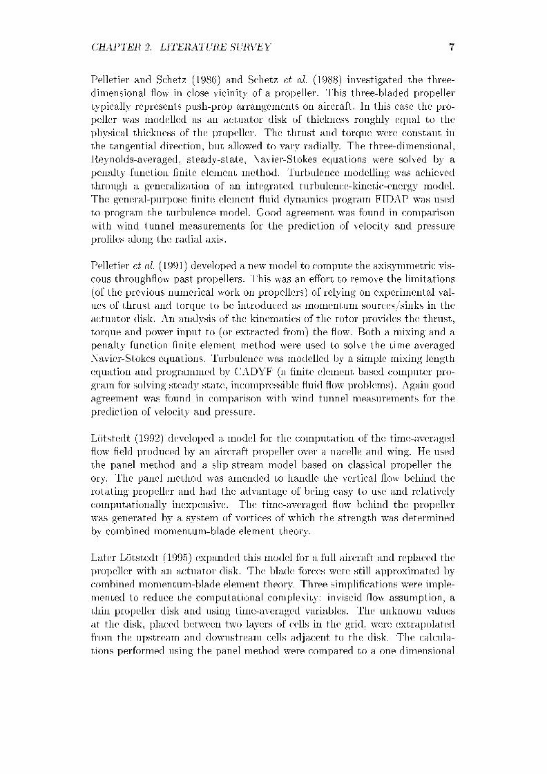
Pelletier and Schetz (1986) and Schetz et al. (1988) investigated the three-dimensional �ow in close vicinity of a propeller. This three-bladed propellertypically represents push-prop arrangements on aircraft. In this case the pro-peller was modelled as an actuator disk of thickness roughly equal to thephysical thickness of the propeller. The thrust and torque were constant inthe tangential direction, but allowed to vary radially. The three-dimensional,Reynolds-averaged, steady-state, Navier-Stokes equations were solved by apenalty function �nite element method. Turbulence modelling was achievedthrough a generalization of an integrated turbulence-kinetic-energy model.The general-purpose �nite element �uid dynamics program FIDAP was usedto program the turbulence model. Good agreement was found in comparisonwith wind tunnel measurements for the prediction of velocity and pressurepro�les along the radial axis.
Pelletier et al. (1991) developed a new model to compute the axisymmetric vis-cous through�ow past propellers. This was an e�ort to remove the limitations(of the previous numerical work on propellers) of relying on experimental val-ues of thrust and torque to be introduced as momentum sources/sinks in theactuator disk. An analysis of the kinematics of the rotor provides the thrust,torque and power input to (or extracted from) the �ow. Both a mixing and apenalty function �nite element method were used to solve the time averagedNavier-Stokes equations. Turbulence was modelled by a simple mixing lengthequation and programmed by CADYF (a �nite element based computer pro-gram for solving steady state, incompressible �uid �ow problems). Again goodagreement was found in comparison with wind tunnel measurements for theprediction of velocity and pressure.
Lötstedt (1992) developed a model for the computation of the time-averaged�ow �eld produced by an aircraft propeller over a nacelle and wing. He usedthe panel method and a slip-stream model based on classical propeller the-ory. The panel method was amended to handle the vertical �ow behind therotating propeller and had the advantage of being easy to use and relativelycomputationally inexpensive. The time-averaged �ow behind the propellerwas generated by a system of vortices of which the strength was determinedby combined momentum-blade element theory.
Later Lötstedt (1995) expanded this model for a full aircraft and replaced thepropeller with an actuator disk. The blade forces were still approximated bycombined momentum-blade element theory. Three simpli�cations were imple-mented to reduce the computational complexity: inviscid �ow assumption, athin propeller disk and using time-averaged variables. The unknown valuesat the disk, placed between two layers of cells in the grid, were extrapolatedfrom the upstream and downstream cells adjacent to the disk. The calcula-tions performed using the panel method were compared to a one-dimensional

CHAPTER 2. LITERATURE SURVEY 8
Euler code and wind-tunnel experiments. The Euler solution provided betteragreement with the wind-tunnel tests at higher Mach numbers, but requireda much �ner grid. The panel method was deemed faster and easier to usefor subsonic �ows, but Lötstedt (1995) preferred the Euler method due to itsability to capture the shape of the slipstream automatically.
Thiart and von Backström (1993) developed an actuator disk model for a lowsolidity/low hub-to-tip ratio axial �ow fan. The Navier-Stokes equations weresolved with the aid of a k − ε turbulence model and the SIMPLEN method.The thrust forces and torque applied on the air �ow by the fan blades were de-termined by blade element theory and the e�ect of distorted in�ow conditionswere investigated. Empirical correlations were used to determine the lift anddrag coe�cients of the blade elements. The method developed by Pericleousand Patel (1986) was followed, hence the lift and drag coe�cients of the bladeelements were used to calculate the lift and drag forces exerted by that spe-ci�c element on the �ow. These forces were then included in the Navier-Stokesequations as body forces. Good agreement with experiments were found butthe increased power associated with distorted in�ow conditions was under pre-dicted.
Van Staden (1996) integrated a fan performance model into a CFD model forthe performance prediction of a complete air-cooled condenser. Experimentalfan performance curves were used to obtain the momentum source term of thefan in the axial direction, which was added to the Navier-Stokes equation as asource term in the CFD model. Good agreement was found with experimentaldata at ideal conditions, but for non-ideal conditions (such as distorted in�ow)the model required the fan performance curves at these adverse conditions.
Meyer (2000) and Bredell (2005) utilized the actuator disk model of Thiart andvon Backström (1993) for their numerical investigations of air-cooled heat ex-changers. As mentioned in the introduction chapter, this model under-predictsthe fan performance at low �ow rates (see Figure 2.1). This can be attributedto the model only taking the axial and tangential velocity components intoconsideration for calculating the relative in�ow vector, neglecting the radialcomponent. The radial component of velocity and the Corriolis e�ect, asso-ciated with rotation, become more prominent at lower �ow rates and inducea delay in boundary-layer separation that results in retarded stall (Ohad andAviv (2005)).
Most of the literature involving axial �ow fans/propellers/impellers revolvearound stirred tanks, propeller propulsion (such as ships and helicopters) andwind turbines. The latter two cases di�er from the work presented here sincethey involve air �ow over unducted fan blades. No previous research in lit-erature could be found for discrete simulation of ducted axial �ow fans used

CHAPTER 2. LITERATURE SURVEY 9
Figure 2.1: ADM compared to experimental data (Van der Spuy et al. (2009)).
in forced-draught heat exchangers. Based on the available literature it canbe concluded that the ADM remains the preferred method for simulating thee�ect of an axial �ow fan on air �ow through ACSC's. The most recent workon the simulation of a stirred tank and one other case of ducted axial fan sim-ulation is presented next.
A complete three-dimensional CFD model was used by Ramasubramanianet al. (2008) to analyse the �ber di�usion process in the manufacturing ofwet-laid nonwovens. The three-bladed impeller and ba�es were modelled inFLUENT� by using the MIXSIM user interface and incorporating the multiplereference frame model. This meant that for the impeller a rotating referenceframe was used and for the ba�es and tank, a stationary reference frame wasused. The impeller has a diameter of 0.2 m and rotates at 350 rpm. A standardk − ε turbulence model was used for the �ow solution. The simulation wascompared to experimental work on a mixing tank with ba�es and an impellerlocated in the center of the tank. The e�ect of a rectangular and triangularcross section on dispersion quality was predicted by the CFD model. Theba�es in this application reduce the recirculating �ow by e�ectively breakingup the large central vortices produced by the impeller. The authors foundthe model useful to predict the location, source and mechanism behind theformation rope and log defects.
Kelecy (2000) predicted the fan performance of a four-bladed axial �ow pro-peller over a range of �ow rates and compared the results with wind tunneldata. The blade has a rotational speed of 2000 rpm and a diameter of 0.11 m.The rotating reference frame method of FLUENT� was used to simulate the

CHAPTER 2. LITERATURE SURVEY 10
rotation of the 14
thaxisymmetric fan model. The �ow equations were solved in
the rotating reference frame. A zero velocity was imposed on the blade sur-faces and shaft, while the outer walls of the tunnel were rotated at the speci�edspeed in the opposite direction when viewed from a stationary reference frame.He observed the sensitivity of the �ow solutions to initial conditions, signi�-cant pressure gradients from the blades to the inlet at lower �ow rates as wellas radial out�ow from the fan as the �ow rate decreases.
2.1.2 Experimental
The accuracy of the CFD model is veri�ed with experimental results. To en-sure con�dence in a set of experimental data, the data set needs to conformto certain air performance test methods (standards), in this case for industrialfans. These standards aim to provide a speci�ed environment where the fanscan be tested. When comparing di�erent fan designs for a certain application,the fan test results all need to adhere to similar conditions, standardized setupand testing procedures to eliminate any uncertainties in the comparison. Thefan test standards, extensively used at the low speed fan test facility at Stellen-bosch University for previous work as well as in this dissertation, is the BritishStandards, BS 848 : Part 1 : 1980. The Type A standard installation type isused, with free inlet and outlet. The fan exhausts into open atmosphere. Thecharacteristics required for fan performance set forth in the BS 848 standards1980, are the fan static pressure rise, the fan power and fan static e�ciency (arelation of the aforementioned two).
Venter (1990) designed the test facility according to the BS 848 standards 1980for testing axial �ow fans. The facility was used to investigate the performanceof axial �ow fans in ACSC's. He looked at the in�uence of �ow distorting fac-tors (such as support structures and heat exchanger con�gurations) and fandesign parameters (such as blade tip clearance and hub plates) on the perfor-mance of a typical industrial cooling fan that he referred to as the V-fan.
From Venter (1990)'s research it became apparent that the V-fan su�ered froma large amount of recirculating �ow in the hub region. Bruneau (1994) set outto resolve this issue and improve on the e�ciency, while maintaining the origi-nal fan pressure rise and volumetric �ow rate, by designing two prototype fanswith a higher hub-tip ratio than the V-fan. The B1-fan utilizes the Clark-Yaerofoil pro�le and the B2-fan incorporates the NASA LS series. Bruneau(1994) mentions that the choice of the NASA LS series blade pro�le was mo-tivated by the particular pro�le's exceptional lift/drag characteristics, goodo�-design performance and its tolerance to inlet �ow distortion. The bladeswere designed with the use of simple radial equilibrium equations. The twofans compared favourably with the fan from Venter (1990) over the entire fanoperating envelope. The fan performance characteristics of the B2-fan with

CHAPTER 2. LITERATURE SURVEY 11
the NASA LS series airfoil pro�le serves as reference data for the experimentalwork carried out in this thesis.
An incident occurred in which the V-fan was destroyed and it was replacedby Stinnes (1998) with the geometrically similar S-fan. Stinnes (1998) inves-tigated the e�ect of a cross-�ow component at the inlet on the performanceof axial �ow fans. For this he incorporated the prototype B1-fan and B2-fanof Bruneau (1994) along with the S-fan and in addition provided a thoroughguideline for performing experimental tests on the test facility at StellenboschUniversity. Furthermore he measured the �ow �eld immediately up- and down-stream of the fan with a 5-hole probe and developed a prediction model topredict local �ow patterns for cases that where not examined with the 5-holeprobe experiments. The method of the prediction model is similar to the ac-tuator disc theory and takes fan blade and local �ow patterns at various radialstations and circumferential positions into account to determine global fanperformance.
Meyer (1996) experimentally investigated a number of component and geomet-rical changes to ACHE's in order to determine the e�ect of these changes onthe ACHE performance characteristics. Two of the changes that are of partic-ular interest were the use of di�erent fan types and fan sizes, and the variationin the fan rotor axial position within the shroud. The necessity to investigatethese two parameters led to another data set of fan performance characteristicsfor the B2-fan for possible use as reference regarding the experimental workwithin this thesis. Meyer (2000) also performed experimental veri�cation ofhis axial �ow fan model with the B2-fan designed by Bruneau (1994).
The fan test facility stood dormant for �ve years, after which it was recom-missioned by Esterhuyze (2006). Unfortunately Esterhuyze (2006) had anincident where the original B2-fan was destroyed and a new set of blades fromthe same mould designed by Bruneau (1994) was manufactured by anotherstudent (Dippenaar, 2007).
The main fan rotor dimensions and set-up of the facility is shown in Figure 2.2.Changing the fan axis position (in an upstream direction) had no discerniblee�ect on the fan performance characteristics (Meyer, 1996); therefore the fanaxis position was kept constant throughout the experiments. The blade staggerangle (ξ) is set relative to the plane perpendicular to the axis of rotation (seeFigure 2.3). To set the blades at a prescribed blade stagger angle, a bladesetting angle (φ) was used in conjunction with a digital projector �xed ontoa blade angle setting jig. The B2-fan speci�cations are given in Table 2.1(Bruneau, 1994).

CHAPTER 2. LITERATURE SURVEY 12
Figure 2.2: Main fan rotor dimensions and set-up, adapted from Meyer (1996).
Table 2.1: B2-fan speci�cations
Number of blades 8Hub diameter (dH) [m] 0.617Fan casing diameter (dFC) [m] 1.542hub-tip ratio 0.4Fan axis position (xF) [m] 0Tip clearance [mm] 3Average chord length [m] 0.167
2.2 Summary of main �ndings
The ADM model provides a means to e�ectively simulate a complete ACHEconsisting of multiple fan units, without using a discrete fan model. This ap-

CHAPTER 2. LITERATURE SURVEY 13
Figure 2.3: Blade stagger angle and blade setting angle.
proach saves computational grid complexity and computer processing power,resulting in reduced time required to obtain a solution. Unfortunately thismodel under-predicts the fan performance at very low �ow rates (Ohad andAviv (2005) and Van der Spuy et al. (2009)). This necessitates a detailed in-vestigation of �ow over the fan blade surfaces in order to amend the existingADM model with the appropriate source terms. Although excellent experi-mental tests (in particular by Stinnes (1998)) were performed on the B2-fanin the past, replacement of the B2-fan blades warrants a new fan performancedata set. The data from Stinnes (1998) did not include fan performance testsat 3 mm tip clearance as referenced by Bruneau (1994). The new fan perform-nce data set would include both tip clearances for reference with previous work.

Chapter 3
Numerical modelling
3.1 Introduction
The analysis of CFD problems generally involve three steps:
� Discretization of the �ow domain
� Setting up and initiating the �ow computation
� Visualizing the results
For these three steps NUMECA has developed three software systems. The dis-cretization is performed in an Automated Grid generator for turbomachinerysystems (AutoGrid�) and/or in an Interactive Geometry modeller and Gridgeneration system for multiblock structured grids (IGG�). The second step isexecuted by the �ow solver EURANUS (EURopeanAerodynamicNUmericalSimulator), which is a three-dimensional multiblock �ow solver that is able tosimulate Euler or Navier-Stokes (laminar or turbulent) �ows. The �nal step isperformed with a highly interactive Computational Field Visualization soft-ware system (CFView�). All three software systems have been integrated intoNUMECA's Flow INtegrated Environment (FINE�), which is a user friendlyGUI, that operates on a project basis eliminating the need for �le manipula-tion in the consolidation of the three steps. Detailed discussions of the threesteps follow.
3.2 Fan blade data
All analyses were performed on what Bredell (2005) referred to as the B-fan.The B-fan is actually the B2-fan designed by Bruneau (1994). The reasonfor choosing the B2-fan is based on the availability of original design data forthe fan. In order to compare a full three-dimensional CFD simulation of theaxial �ow fan to the experimental results, the same data for the blade pro�le
14

CHAPTER 3. NUMERICAL MODELLING 15
had to be used. Bruneau (1994) designed the blade with a linear decrease inblade thickness of 13 % (thickness/chord ratio) at the hub down to 9 % at thetip. To de�ne the change in blade properties from hub to tip, the blade wasdivided into several two-dimensional sectional blade pro�les at di�erent radialstations. To calculate the blade pro�le co-ordinates the chord length and stag-ger angle at each radial station is needed. After scaling the chord length at thehub and tip radius, Bruneau (1994) used linear interpolation to determine thechord length at the intermediate radial stations. The stagger angle is deter-mined from the di�erence between the inlet relative �ow angle and the angleof attack. The angle of attack for each radial station was interpolated from aC-spline �tted through experimentally determined angle of attack versus liftcoe�cient data, for the particular airfoil pro�le used in the fan blade design.Figure A.1 in Appendix A shows the distribution of chord length and staggerangle radially across the blade length.
Bruneau (1994) used the General Aviation (Whitcomb)-number two (GA(W)-2) airfoil designed by McGhee et al. (1977), as a pro�le for the blades of theB2-fan. The GA(W)-2 is a 13 % thick airfoil derived from the 17 % thickGA(W)-1 airfoil originally designed for propeller driven light aircraft. The13 % thick GA(W)-2 airfoil is obtained by linearly decreasing the mean thick-ness distribution of the 17 % thick GA(W)-1 airfoil with a ratio of 13
17.
McGhee et al. (1977) produced an airfoil pro�le data set, as used by Bruneau(1994), of 39 points per surface. Using this data set rendered a coarse mesh,observed after generating the mesh in IGG�. Further investigation revealedthat a whole family of airfoils emerged from the GA(W)-1 airfoil with a newdesignation, resulting in the GA(W)-1 airfoil becoming the LS(1)-0417 and theGA(W)-2 airfoil becoming the LS(1)-0413 airfoil. According to McGhee et al.
(1979) the LS(1) designates low speed (�rst series); the �rst two digits specifythe airfoil design lift coe�cient in tenths, while the last two digits indicatethe airfoil thickness in percent chord. McGhee et al. (1979) produced a �nerairfoil pro�le data set of 45 points per surface. Figure A.2 displays a plot ofthe GA(W)-2 pro�le and the LS(1)-0413 pro�le from the di�erent data sets.
Seven airfoil pro�le data sets were produced at di�erent radial stations fromthe 45-point-per-surface data. These radial station blade co-ordinates wereused in the mesh modelling by importing the data set into IGG� and �ttinga C-spline through the data. From this C-spline 200 data points per surfacewere exported to a data �le for use in the three-dimensional blade generationprocess in AutoGrid�. Table A.1 displays the fan blade data set for the hubpro�le. A close-up view of the grid resolution at the blade leading edge isillustrated in Figure 3.1.

CHAPTER 3. NUMERICAL MODELLING 16
Figure 3.1: Leading edge grid point distribution.
3.3 Computational domain
A 18
thdiscrete three-dimensional computational grid for an axial �ow fan was
developed using a combination of the AutoGrid� and IGG� software from NU-MECA. The AutoGrid� software facilitates fully automated grid generation forturbomachinery blades, while the IGG� software is a powerful structured gridgenerator. The model consists of three segments, namely the inlet, blade andoutlet segments. Both the inlet and outlet segments were created in IGG�,while AutoGrid� was used for creation of the more complex blade geome-try. Once all three segments were completed separately, they were combinedwithin AutoGrid� with the use of three-dimensional technological e�ects toform a single model. Three-dimensional technological e�ects in AutoGrid�include all e�ects de�ned by three-dimensional surfaces or three-dimensionalcurves whose meshes were created manually in IGG�. This single model wasreopened in IGG� for the �nal speci�cation of the rotor-stator interface be-tween the blade segment and the inlet segment on one side as well as the outletsegment on the other side.
3.3.1 AutoGrid�
The approach stipulated in the user manual (AutoGrid� Manual, 2007a) wasfollowed for semi-automatic three-dimensional blade generation. This included:
1. De�nition of the geometry. This includes speci�cation of the blade pro-

CHAPTER 3. NUMERICAL MODELLING 17
�le surfaces from the imported data of Table A.1 in Appendix A, aswell as specifying the hub and shroud surfaces of revolution. Additionalinformation such as tip clearance (3 mm in this case) is also speci�ed.
2. Generation of meridional �ow paths. These paths act as meridionaltraces for the surfaces of revolution on which the three-dimensional meshis built.
3. Generation and control of the two-dimensional mesh on the surfaces ofrevolution. This allows the manipulation of the mesh topology and gridclustering. The grid quality can be checked at di�erent radial stations.
4. Generation of the �nal three-dimensional mesh. The three-dimensionalmesh is generated by using conformal mapping between the three-dimensionalCartesian space and the two-dimensional meshes on the surfaces of rev-olution that follows the meridional �ow paths.
The AutoGrid� interface allows checking of the mesh quality at any level, radi-ally between the hub and the shroud. The mesh quality is measured accordingto the following criteria:
� Orthogonality, the measure of the skewness of the cells and is determinedby the minimum angle between the edges of the cell. It has a range of0◦ to 90◦.
� Angular deviation, the measure of the angular variation between twoadjacent cells in all directions. It has a range of 0◦ to 180◦.
� Aspect ratio, the measure of how thin (ratio of width to length of thecells) a cell is. It has a range of 1 to 50000.
� Expansion ratio, the measure of the size variation between two adjacentcells in a speci�c direction. It has a range of 1 to 100.
� Cell width, i.e. the height of the cell measured in all directions. It has arange of 0 m to 1 000 000 m.
A check for negative cells is also performed at this stage.
The mesh quality can be improved by controlling the selected topology. Au-toGrid� has three prede�ned topologies. The HHOHH (O4H) topology allowsfor full automatic meshing for all kinds of turbomachinery geometries; whilethe HOH and H&I topologies ensure very high quality grids, but according tothe user manual (AutoGrid� Manual, 2007a) are not suitable for all applica-tions. In the generation of the three-dimensional mesh for the axial �ow fanthe default O4H topology is used. The O4H topology allows control of �veblocks (referring to Figure 3.2):

CHAPTER 3. NUMERICAL MODELLING 18
Figure 3.2: O4H topology blocks and grid points, (AutoGrid�Manual, 2007a).
1. an O-block around the blade called the skin block
2. an H-block upstream of the blade leading edge called the inlet block
3. an H-block downstream of the blade trailing edge called the outlet block
4. an H-block above the blade section called the up block
5. an H-block below the blade section called the down block
By altering the number of grid points in the di�erent blocks the mesh qualitycan be improved accordingly. Once the required mesh quality is achieved, theAutoGrid� �le is saved, allowing for automatic regeneration of the blade withthe speci�ed grid points at a later stage if needed.
3.3.2 IGG�
Both inlet and outlet segments were created by projecting blocks from a sur-face geometry. These projected blocks were revolved 45° around the Z-axis to
create a 18
thaxisymmetric model. The number of grid points in all three direc-
tions was speci�ed at this stage. Once the required mesh quality is achieved,the clustering of cells near surfaces to be de�ned as walls was attempted. IGG�(IGG�Manual, 2007c) uses the same mesh quality criteria as AutoGrid� (Au-toGrid� Manual, 2007a). The clustering of cells speci�es the cells distribution

CHAPTER 3. NUMERICAL MODELLING 19
in any direction normal to a surface. To achieve low y+ values, dense cell dis-tribution (clustering) close to a wall surface is necessary. The IGG� interfaceallows the creation of segment groups with the same clustering to ease andautomate the process of adjusting cell clustering. Some clustering near thefan exit was implemented where high velocity gradients were expected. Thisstep requires the mesh quality to be checked again, since the blocks need tobe regenerated to accept the clustering changes.
After completing the geometry block generation and setting the periodicityfor eight blades the various boundaries were speci�ed. This includes outlet,inlet as well as solid wall boundaries. At this stage the connecting surfacessurrounding the bellmouth blocks on the inlet segment were changed to solidwall surfaces to accommodate attaching the bellmouth inlet to the fan segment.
3.3.3 Domain speci�cations
The complete computational domain consists of three main sections, namelythe inlet to the fan, the fan rotor and the outlet. The inlet and outlet sectionsconsist of a structured mesh generated in IGG�, including all boundary condi-tions and periodicities. The blade and the endwalls (hub and shroud) formingthe fan rotor part of the model, were generated in AutoGrid�, including set-ting the periodicities. All three complete sections were integrated into a singlemodel for the complete CFD simulation of the fan test facility by adding theinlet and outlet to the fan blade model in AutoGrid�. Saving this �le createsan *.igg �le (which can be manipulated within IGG�) that is integrated in theFINE� interface to be coupled with the EURANUS �ow solver. A detaileddiscussion of the three sections follows.
Essentially two computational domains were evaluated. Both domains sharedthe same inlet and blade section, but utilized di�erent outlet sections. The�rst CFD model contains a pinched outlet section and will be addressed asApproach-1. The second model with an open outlet will be addressed asApproach-2. The two models consists of the same amount of grid cells, namely4728631 cells. Figure 3.3 displays an azimuthal view of the �rst model withthe general grid dimensions. An isometric view of the complete computationaldomain for the �rst model is illustrated in Figure 3.4. Figure 3.5 presentsthe general grid dimensions of the second model and an isometric view of thesecond model is presented in Figure 3.6. The fan diameter is denoted by dF .

CHAPTER 3. NUMERICAL MODELLING 20
Figure 3.3: Azimuthal view of computational domain dimensions, Approach-1.
Figure 3.4: Isometric grid view of computational domain, Approach-1.

CHAPTER 3. NUMERICAL MODELLING 21
Figure 3.5: Azimuthal view of computational domain dimensions, Approach-2.
Figure 3.6: Isometric grid view of computational domain, Approach-2.

CHAPTER 3. NUMERICAL MODELLING 22
3.3.3.1 Inlet
The inlet section of the computational domain is geometrically true to thetest facility dimensions beyond the mesh screens inside the settling chamberand includes the bellmouth inlet to the fan. Instead of modelling the settlingchamber with a square inlet the hydraulic diameter of the settling chamberwalls was calculated and used. This option is implemented to coincide withthe eight-segment axisymmetric nature of the CFD model. Equation (3.3.1)shows the calculation of the settling chamber hydraulic diameter based on theprinciple of equal �ow area. An isometric view of the inlet section, containing1483560 cells, is illustrated in Figure 3.7. Non-rotating solid wall boundariesare speci�ed for all walls, except at the 0.05 m inner radius, where an Euler(zero-shear) wall is used. According to White (2006) for a �xed Euler wallthe no-slip condition is dropped and the tangential velocity allowed to slip.These solid wall boundaries can be seen in Figure 3.8. The inlet boundaryis mass�ow imposed and a rotor-stator interface is assigned to the patch thatis coupled with the fan rotor section. The remaining boundaries are set to
periodic boundaries for a 18
thaxisymmetric model.
dh =
√4 b h
π
=
√(4)(3.7)(3.7)
π= 4.175 m (3.3.1)
3.3.3.2 Blade
The grid point distribution on the O4H-topology is shown in Figure 3.2. Thisleads to a total of 1106311 grid points for the fan blade, hub and shroud. Atip-gap of 3 mm is incorporated in the fan blade section. A fully generatedblade is displayed in Figure 3.9. The cell blocks containing the tip gap is notshown.
In order to capture the high gradients of velocity within the boundary layer,an adequate amount of cells should be placed within the boundary layer. Thewall variable commonly used to evaluate this is the y+ value. The y+ valueassociated with the �rst node o� the wall is given in equation (3.3.2), accord-ing to the FINE�/Turbo Manual (2007b).
y+1 =
ρ uτ yw
µ(3.3.2)

CHAPTER 3. NUMERICAL MODELLING 23
Figure 3.7: Isometric grid view of computational domain inlet section.
Figure 3.8: Isometric grid view of computational domain inlet section solidboundaries.

CHAPTER 3. NUMERICAL MODELLING 24
Figure 3.9: A single blade generated in AutoGrid�.
Here yw is the height of the �rst grid node o� the wall and uτ is the frictionvelocity de�ned by
uτ =
√τwρ
=
√1
2U2ref Cf (3.3.3)
with τw the wall shear stress, Uref the reference velocity and Cf the shearcoe�cient.
Di�erent turbulence models for Low- and High-Re number �ows require di�er-ent ranges of y+
1 values to accurately predict the boundary layer. To achievethis, the correct range of y+
1 values per turbulence model need to be obtained.The FINE�/Turbo Manual (2007b) speci�es that for Low-Re turbulence mod-els solving the viscous sublayer (y+
1 ≤ 5, White (2006)), y+1 values between
1 and 10 is acceptable. The FINE�/Turbo Manual (2007b) also recommendsusing a Low-Re turbulence model if separation is expected, since the logarith-mic function does not apply for separated �ow. Since the y+
1 value dependson the value of yw, according to equation (3.3.2), it can be used to control thecorresponding y+
1 values based on the truncated series solution of the Blasius

CHAPTER 3. NUMERICAL MODELLING 25
equation (FINE�/Turbo Manual, 2007b):
yw = 6
(Urefν
)− 78(Lref
2
) 18
y+1
= 6
(1.5
1.511× 10⁻⁵
)− 78(
0.167
2
) 18
(5)
= 9.335×10⁻⁴ (3.3.4)
where Uref can be taken as the average inlet velocity, ν the kinematic viscosityand Lref the reference length (taken as the blade chord length). The y+
1 valuefor the blade is well within the 1 to 10 range (y+
1 ≤ 9.551), and only reachesthe limit of 10 near the tip gaps (Figure 3.10). This was deemed su�cientsince the tip clearance �ow consists of highly accelerating �uid and is di�erentfrom a normal boundary layer.
(a) y+1 range 1 to 10. (b) y+
1 range 1 to 5.
(c) y+1 near tip gap.
Figure 3.10: y+1 values for the blade section.
Non-rotating solid wall boundaries are speci�ed for the shroud. The blade andhub are assigned solid surfaces rotating at 750 rpm. The patches connecting

CHAPTER 3. NUMERICAL MODELLING 26
the inlet and outlet sections to the fan rotor sections are speci�ed as rotor-stator interfaces. The remaining boundaries are set to periodic boundaries for
a 18
thaxisymmetric model. Figure 3.11 gives an indication of the axisymmetric
nature of the CFD model.
(a) 18
thaxisymmetric model, without repe-
tition.(b) 1
8
thaxisymmetric model, with repeti-
tion.
Figure 3.11: Axisymetric nature of CFD model.
3.3.3.3 Outlet
The fan test facility on which the computational domain is based, houses a fanthat exhausts into the open atmosphere. De�ning such an �open atmosphere�outlet within a computational domain is problematic. To keep the integrityof the model intact would require outlet patches in both the axial and radialdirections. This opens the possibility for a large amount of back�ow to enterthe domain at the outlet boundary and severely destabilize the simulation.The support team at NUMECA strongly advised against using such an �open�outlet and deemed any results obtained from such simulations untrustworthy.To resolve this issue the outlet is pinched for Approach-1, some distance awayfrom having an in�uence on the fan performance. The only objective of thepinching is to increase the local velocity in this region and to restrict theback�ow over the outlet. The static outlet pressure is not taken at the pinchedoutlet, but rather averaged over a series of surfaces, on the constant z-plane,before the pinching in the model commences. The static pressure value of eachsurface is an averaged value for the static pressure over the particular area.Figure 3.12 shows a plot of these surfaces. To resolve the radial out�ow issue,Euler walls are implemented at the endwalls of the outlet. With the no-slipcondition removed for Euler walls, they only prohibit the �ow from exiting themodel, thus aiding the pinching e�ect. The Euler walls are placed su�ciently

CHAPTER 3. NUMERICAL MODELLING 27
far away from the fan rotor.
Figure 3.12: Averaged surfaces for obtaining outlet pressure.
Similar to the inlet, the patch connecting the outlet section with the fan rotoris speci�ed as a rotor-stator patch. The patch coinciding with the outside wallof the settling chamber is de�ned as a solid wall. The remaining patches areassigned Euler walls, referring to the discussion earlier. A radial equilibriumstatic pressure is enforced at the outlet patch with atmospheric pressure im-posed at the outer circumference. The complete computational domain, of2138760 cells, is illustrated in Figure 3.13.
The outlet section for Approach-2 avoids the use of a pinched outlet and zero-shear Euler walls. The circumferential outlet patch employs a static pressureboundary condition. The outlet patch on the plane normal to the fan axisimposes a radial equilibrium static pressure boundary condition, similar to theoutlet section of Approach-1. Both outlet sections contain the same amountof cells and are connected to the fan rotor via a rotor-stator interface. Thecomplete computational domain is presented in Figure 3.14.
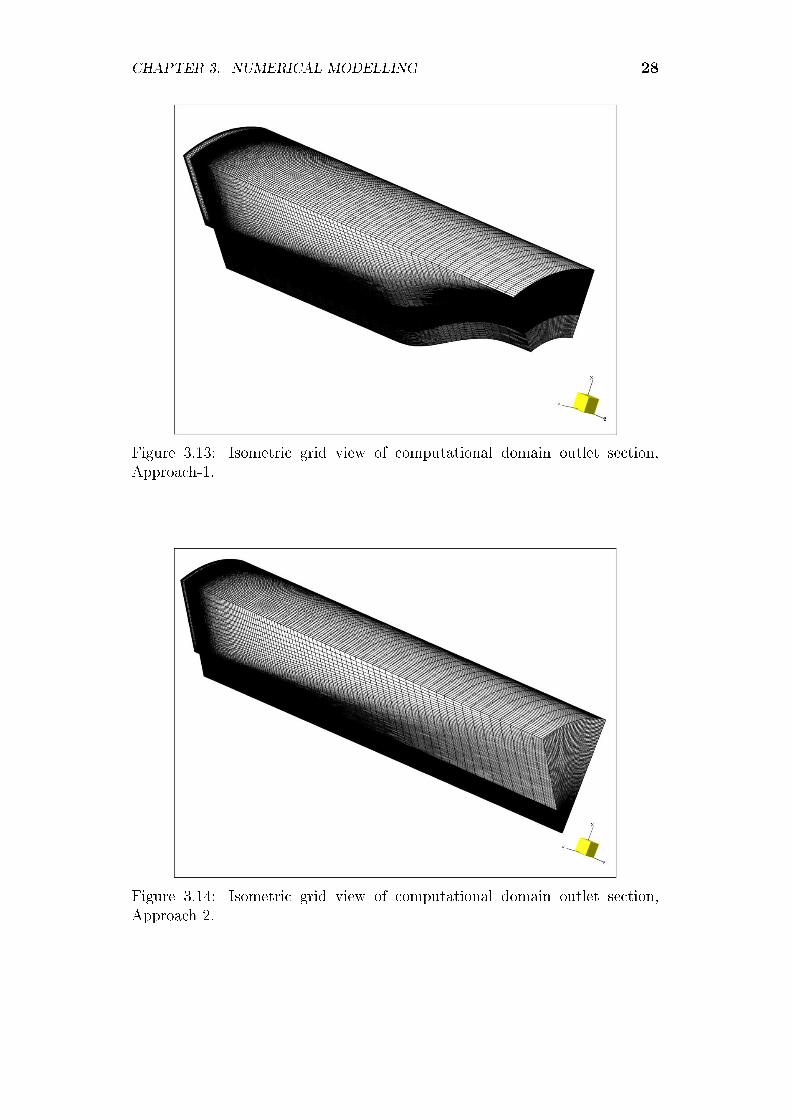
CHAPTER 3. NUMERICAL MODELLING 28
Figure 3.13: Isometric grid view of computational domain outlet section,Approach-1.
Figure 3.14: Isometric grid view of computational domain outlet section,Approach-2.

CHAPTER 3. NUMERICAL MODELLING 29
3.4 Computational parameters
All the parameters necessary to set up and facilitate a steady-state �ow sim-ulation are discussed in detail.
3.4.1 Fluid Model
Within FINE� it is possible to choose a �uid type from a pre-de�ned databaseor create a new �uid type. The pre-de�ned database contains the followingtypes of �uids: perfect gas, real gas, incompressible gas or liquid and condens-able �uid.
After researching the user manual it became apparent that FINE�'s real gasis actually a thermally perfect gas and the perfect gas a calorically perfectgas. According to Anderson (1990) a true real gas has an equation of statethat takes compressibility e�ects, variable heat capacity, Van Der Waals forces,non-equilibrium thermodynamic e�ects and issues with molecular dissociationand elementary reactions into account. This is a very extensive analysis andvarious simpler gas laws exist. The ideal gas law simpli�es the real gas byassuming a compressibility factor of one. White (2006) stipulates that �allcommon gases follow with reasonable accuracy, at least in some �nite region,the so-called ideal or perfect gas law�. Furthermore a perfect gas can be de�nedas one where the intermolecular forces of the real gas are neglected to simplifycalculations. Anderson (1990) states that this perfect gas simpli�cation canbe further simpli�ed and classi�ed as a thermally perfect gas and a caloricallyperfect gas.
The thermally perfect gas assumes that the gas is in thermodynamic equilib-rium, not chemically reacting and that internal energy, enthalpy, and speci�cheats are functions of temperature only. The calorically perfect gas enforcesall the assumptions of the thermally perfect gas, but assumes constant speci�cheats. In FINE� the perfect gas model assumes constant speci�c heat (Cp)and constant speci�c-heat ratio (γ).
For the incompressible �uid type the density can either be constant or a pre-de�ned function of the pressure. Using air as an incompressible gas in thedefault FINE� setting, the density law is de�ned by the Boussinesq law, inwhich case the density is kept strictly constant. With no terms in the massand momentum equations depending on the temperature, these conservationequations are decoupled from the energy conservation equation.
Relative stable �uid temperature meant that the use of the real gas (thermallyperfect gas) �uid type was not considered. The perfect gas (calorically perfectgas) and incompressible �uid types were investigated and a fan static pressure

CHAPTER 3. NUMERICAL MODELLING 30
rise error amongst the two �uid types of less than 3 % was found. Howeverthe incompressible �uid type required almost double the amount of iterationsto give answers that correlate with the perfect gas �uid type. Therefore theperfect gas model was used for the axial �ow fan model.
3.4.2 Flow Model
For this model steady �ow is assumed and time independent �ow calcula-tions are solved. This investigation considers a one-equation turbulence model,namely Spalart-Allmaras (Spalart and Allmaras, 1994). The Spalart-Allmarasturbulence model is NUMECA's default model, providing good convergence forcommon turbomachinery applications (FINE�/Turbo Manual, 2007b). TheSpalart-Allmaras turbulence model performs considerably better than the al-gebraic turbulence models, such as the Baldwin-Lomax model, especially inmapping the performance of separated �ow (Ashford and Powell, 1996). Themodel is also more robust, computationally less expensive and requires lessmemory than the two-equation k − ε turbulence model (Ashford and Powell(1996). Both models employ constant Prandtl numbers.
3.4.3 Rotating Machinery
FINE� allows the user to specify rotating blocks and rotor-stator interfacesto accommodate rotating and non-rotating sections within a domain. In thismesh the blocks were all set to be rotating while the relevant solid surfaces,such as the shroud and settling chamber walls, were kept stationary. This ap-proach is somewhat similar to that used by Kelecy (2000) who kept the bladesand shaft stationary, while maintaining an angular velocity at the outer wallsin the opposite direction from the supposed blade rotation.
An attempt was made to utilize the classic turbomachinery simulation ap-proach where only the blocks containing the rotor were allowed to rotate, keep-ing the remaining blocks stationary. In this instance two rotor-stator interfacetypes, the mixing plane approach and the frozen rotor, were investigated:
� With the mixing plane approach circumferentially averaged �ow quanti-ties (such as mass, momentum and energy �uxes) are exchanged at therotor-stator interface. According to the FINE�/Turbo Manual (2007b)a more strict global conservation through the interface is achieved whenusing a �ux based approach instead of exchanging the classical primi-tive variables. Thus any blade wake or separation is mixed circumfer-entially before entering the downstream component, resulting in a cir-cumferentially uniform pressure distribution as well as uniform velocitycomponents at the interface. The static pressure distribution over therotor-stator can be viewed in Figure 3.15.

CHAPTER 3. NUMERICAL MODELLING 31
Figure 3.15: Static pressure distribution over the mixing plane approach rotor-stator interface.
� With the frozen rotor approach no mixing of the �ow solution at the in-terface occurs. Instead the rotor movement is neglected and the upstreamand downstream components can be seen as being literally connected.Thus the continuity of the velocity components and pressure is imposedon the interface. The governing equations for the rotor are solved in arelative reference frame, and that of the stator in an absolute referenceframe. The �ow solution is thus dependent on the relative position ofthe rotor and stator sections. The static pressure distribution over therotor-stator can be viewed in Figure 3.16.
Unfortunately neither of the aforementioned methods provided satisfactory re-sults. For Approach-1 the mixing plane approach delivered the closest resultscompared to the experimental data with a 28.7 % error in fan static pressurerise at the design operating point. This was only achieved after 18234 itera-tions with a very unstable simulation. The frozen rotor approach was morestable, but could only achieve a 53.82 % error in fan static pressure rise com-pared to experimental data. The aforementioned results were produced with azero-order extrapolation of �ow quantities from inner cells to the rotor-statorinterface. Using �rst-order extrapolation provided somewhat better results ata 111-grid-level (coarser mesh), but it was too unstable at a 000-grid-level(�nest mesh) and the simulations could not complete more than 1000 itera-tions before diverging, for both cases.
One of the problems with using the aforementioned approach, is the mixing

CHAPTER 3. NUMERICAL MODELLING 32
Figure 3.16: Static pressure distribution over the frozen rotor rotor-statorinterface.
losses introduced at the rotor-stator interfaces due to the �ow being forcedto mix out in a short distance, where normally it would have had an in�nitedistance to do so. The mixing losses over the rotor-stator interface can rangeanywhere from 10 Pa to 100 Pa; which is small enough to be neglected in tur-bomachinery applications with a big pressure rise. However, in this applicationit is an order of magnitude of the pressure capability of the axial �ow fan andin�uences the fan performance considerably.
Another issue unique to the axial �ow fan is the amount of back�ow observedat the rotor-stator interface. The back�ow increases signi�cantly at lower�ow rates and is a major source of unsteadiness in the simulation. With themixing plane approach the azimuthal averaged �ow quantities on the down-stream side of the blade outlet rotor-stator interface contains back�ow and isdi�erent from the �ow quantities on the upstream side. To resolve this issuethe rotor-stator interface would need to be placed far enough downstream toavoid having back�ow over the interface. This would also allow the �ow tomix out naturally before reaching the interface, therefore eliminating mixinglosses. In e�ect this is what has been done in the current model, where therotor-stator interfaces have essentially been moved all the way to the inlet andoutlet boundaries. Having no stator-like structures in the geometry of the ax-ial �ow fan, neglecting the need for a rotor-stator interface in the �ow domain,the error introduced by allowing all the blocks to rotate is small.
The aforementioned simulation approach is commonly used for three-dimensional

CHAPTER 3. NUMERICAL MODELLING 33
wind turbine simulations (Sezer-Uzol and Long, 2006).
3.4.4 Boundary Conditions
FINE� allows the speci�cation of �ve di�erent types of boundary conditions:inlet, outlet, solid walls, periodic and external (far �eld).
The use of a mass �ow and static temperature imposed inlet boundary andstatic pressure outlet boundary for the axial �ow fan was advised per emailcorrespondence with the NUMECA support team and mentioned as the ad-visable setup for compressible or low-speed �ows in the FINE�/Turbo Manual(2007b). According to the manual this setup stabilizes the �ow calculationsand provides better initial solutions for multistage calculations.
At the inlet boundary the mass �ow is imposed through a speci�ed controlsurface consisting of related patches grouped together. With this boundarycondition the velocity vector and temperature is imposed on the same controlsurface. For the velocity vector either the swirl and the direction of the ve-locity vector in the meridional plane or the direction of the absolute velocityvector can be imposed. The latter was enforced since no swirl is expected atthe inlet boundary which coincides with the exit of the mesh screens in thesettling chamber of the fan test facility. The absolute velocity vector is speci-
�ed in the axial direction:
(Uz| U |
= 1
). The static temperature can either be
speci�ed as a constant or as a relation between the inlet static pressure andthe average static pressure along a speci�ed outlet. The latter option is notapplicable to the current setup as it requires the mass�ow imposed at bothinlet and outlet boundaries. Furthermore, the turbulent viscosity µt for theSpalart-Allmaras turbulence model need to be speci�ed at the inlet boundary.All speci�ed values are absolute quantities.
Imposing static pressure at the outlet boundary can be done with three di�er-ent methods:
1. Imposing a uniform static pressure across the control surface. For thiscase the static temperature and velocity components at the boundaryare extrapolated from the nearest control volumes.
2. Imposing an average pressure across the control surface. The averagestatic pressure is speci�ed and instead of a uniform pressure distributionthe pressure pro�le is extrapolated from the inner cells and translated toensure the average pressure value that was speci�ed is met at the controlsurface.
CHAPTER 3. NUMERICAL MODELLING 34
3. Using radial equilibrium. Since this model has a cylindrical outlet withmesh lines at constant radius the static pressure can be imposed at a con-stant radius (the outer radius in this case). The hub-to-shroud pressurepro�le is then calculated by integrating the radial equilibrium equation(3.4.1) in the spanwise direction with pitchwise averaged values of vθ andr.
∂p
∂r= ρ · v
2θ
r(3.4.1)
The option of using radial equilibrium provided the best results.
The velocity and thermal conditions for solid wall patches are de�ned usingthe solid wall boundary type. The boundary can be either de�ned as zero-slipor zero-shear. The settling chamber walls, shroud and bellmouth surfaces arede�ned as zero-slip walls with a zero rotational velocity. All the rotating sur-faces consisting of the blade and hub surfaces are de�ned as zero-slip walls witha rotational velocity of 750 rpm. All zero-slip walls are de�ned as adiabatic.
All rotating surfaces are utilized to compute the force and torque of the sys-tem. For the cylindrical axial �ow fan model the axial thrust is de�ned as theprojection of the global force on the rotation axis and the couple exerted bythe global force, around the rotational axis of the fan, as the torque. The axialthrust is computed from the pressure and velocity �elds of the �uid acting onthe blade surfaces according to equation (3.4.2):∑
S
~F · ~nz (3.4.2)
The projection of the torque along a given direction ~z is given by equation(3.4.3).(∑
S
~r × ~F
)· ~z (3.4.3)
3.4.5 Numerical Model
Three computational parameters allow the user to improve the convergencerate of the simulation:
� CFL number
� Multigrid parameters
� Preconditioning parameters

CHAPTER 3. NUMERICAL MODELLING 35
3.4.5.1 CFL number
The Courant-Friedrichs-Levy (CFL) number scales the time-step sizes that areused for the time-marching scheme of the �ow solver. A higher CFL numberleads to faster convergence but can lead to divergence and unstable simulations(FINE�/Turbo Manual, 2007b). The inverse of this is also applicable wherechoosing a smaller CFL number in an unstable simulation improves conver-gence. At the low �ow sections of the fan performance curve, a lower CFLnumber was chosen to improve the convergence of the simulation.
3.4.5.2 Multigrid parameters
For e�ciency and fast convergence the EURANUS �ow solver uses a multigridstrategy in solving the �ow equations on di�erent grid levels. To complementthis, a Full Multigrid Strategy option is also available wherein the solution ofa coarser grid level is used as an initial solution for the next level of �ner grid.
With the �ow solver automatically coarsening the initial mesh from IGG� anoption is available to run simulations on several sub-meshes. The coarsest gridlevel that can be achieved with any mesh depends on the number of timesthe grid can be coarsened along each of the (I, J, K) directions. This numberwould be represented by �n� in equation (3.4.4)
cell size = 2n (3.4.4)
For example, if a grid size is de�ned by 8× 16× 16 cells in the I, J, K directionsrespectively, the mesh can be coarsened to 3,4,4 grid levels in the respectivedirections. Figure 3.17 displays grid level coarsening in one direction. Thesame e�ect on the hub grid distribution around the fan blade can be viewed inFigure 3.18. However, using a hybrid grid level structure as described abovemay deform the mesh in a preferential direction upon coarsening. This mightincrease the aspect ratio for instance and e�ectively reduce the quality of theoverall mesh. In setting up a mesh in IGG� care should be taken to keepa uniform grid level distribution. The �nest grid level is denoted by a 0 inany (I, J, K) direction and the coarser grid levels follow in a numerical order:0,1,2. . . (see Table 3.1 for a grid level display of the previous example). In theaxial �ow fan model three grid levels 222, 111 and 000 were used to obtain a�ow solution.
With the Multigrid Strategy the �ow calculation is performed on all the gridlevels simultaneously in order to speed up convergence. The EURANUS �owsolver implements an explicit multi-stage Runge-Kutta time marching scheme.The number of times the Runge-Kutta operator is applied (number of sweeps)can be speci�ed for each grid level. The coarse grid level to �ne grid levelsweep of the multigrid cycle is initiated once a solution of the coarsest mesh is

CHAPTER 3. NUMERICAL MODELLING 36
Figure 3.17: Mutigrid Strategy.
(a) Finest mesh resolution, 000. (b) Coarser mesh resolution, 111.
(c) Coarsest mesh resolution, 222.
Figure 3.18: Multigrid resolution for the blade hub.
achieved and smoothed. The current solutions on �ner grids are updated withthe solution on the next coarser grid level. This approach leads to an e�cientand fast convergence (FINE�/Turbo Manual, 2007b).

CHAPTER 3. NUMERICAL MODELLING 37
Table 3.1: Grid level distribution.
Grid level Grid points in Number ofnotation I, J, K direction grid points0 0 0 9×17×17 26011 1 1 5×9×9 4052 2 2 3×5×5 753 3 3 2×3×3 183 4 4 2×2×2 8
The option of using a Full Multigrid Strategy provides a good initial solution.A preliminary multi-stage Runge-Kutta explicit scheme is started on the coars-est grid level, but the solution will not be interpolated to the next �ner gridlevel, until a speci�ed convergence is achieved. This solution is then appliedas an initial solution on the �ner grid level for further iterations. The cycleis repeated until the �nest grid level is reached. The grid level at which thepreliminary run should be initiated (level 222 or 111) as well as the numberof iterations to be performed on the corresponding grid level (if convergenceis not achieved) can be speci�ed for each grid. It was found that if conver-gence on coarser grid levels were not obtained it resulted in divergence of thesimulation on �ner grid levels. For the axial �ow fan model care was takento ensure a good level of convergence was achieved before initializing the next�ner mesh with the previous solution. The larger cell size of the coarsest meshleads to a fast convergence, which provides a good initial solution and allowsa more robust simulation on the �nest grid level.
3.4.5.3 Preconditioning parameters
Within FINE� preconditioning is automatically utilized for incompressible�ows and serves as a viable option for other low Mach number �uid typesto improve the convergence rate.
According to the FINE� user manual �when the magnitude of the �ow ve-locity becomes small in comparison with the acoustic speeds, time marchingcompressible codes converge very slowly�. This problem is addressed with theuse of a low speed preconditioner. A preconditioning matrix is multiplied withthe time derivatives of the unknowns that arise in the �ow equations whentime marching algorithms are used to solve steady state applications. Thesetime derivatives have no physical meaning and can be modi�ed without alter-ing the �nal steady state solution. This results in reduced round-o� errors atlow Mach numbers (caused by the use of absolute pressure in the momentumequations) by the introduction of reduced �ow variables such as the dynamic

CHAPTER 3. NUMERICAL MODELLING 38
pressure and the dynamic enthalpy. Also, by using a pseudo-wave speed inorder of magnitude of the �uid speed, instead of the acoustic wave speed, thedi�erence between the convective and the acoustic eigenvalues are lessened.
For the axial �ow fan model Merkle preconditioning was used. The Merklepreconditioner is amongst the most popular used perconditioners and hasbeen extended, from a very e�cient preconditioner for two-dimensional lowMach number �ows, to also solve three-dimensional �ows (Turkel et al. (1997),Zhonghua et al. (2007) and Vigneron et al. (2008)).
3.4.6 Initial Solution
FINE� allows, amongst other, the option to either initialize a computationfrom constant values or from an initial solution �le. In the former case physi-cal values need to be speci�ed that are used uniformly in all the blocks excepton the boundaries. The variables for these values are static pressure, statictemperature and the velocity components. This method of initialization wasused for the coarsest (222) grid level. For the intermediate grid level (111)coarse grid initialization was used where the 111-grid-level computation wasautomatically started from the 222-grid-level computation after a few itera-tions. The 111-grid-level computation was allowed to converge to provide aninitial solution �le to be used in the latter initialization method mentionedearlier. The �nest grid level (000) computation was started from this ini-tial solution �le. Using this approach accelerated the convergence rate andremoved the risk op having a solution diverging at a �ner grid level due tostarting from an unconverged initial solution from a coarser grid level. Usingthis hybrid approach is especially bene�cial at very low �ow rates where alower CFL number is needed. The 222- and 111-grid-level computations canstill be solved with a higher CFL number, for faster convergence, and with theswitch to the �nest grid level (000), a lower CFL number is chosen to stabilizethe computation.
3.4.7 Output
In order to have e�cient memory usage and still retain all the �ow quantitiesof immediate interest, FINE� allows specifying the necessary �ow quantities tobe saved and lets the post-processing package CFView� calculate the derivedquantities. The �ow quantities can either be calculated at all the mesh nodesor along the solid wall boundaries.
3.4.8 Computation Steering and Monitoring
FINE� allows multi-process analyses where the convergence histories of mul-tiple computations can be viewed simultaneously. Utilizing the MonitorTurbo

CHAPTER 3. NUMERICAL MODELLING 39
interface the default quantities for a turbomachinery computation can beviewed independently. The residuals relative to the transport equations arealso made available.
The residuals are calculated as a �ux balance of the �uxes summed on all thefaces of each cell:
RES =∑
fluxes (3.4.5)
The root mean square and the maximum of the residuals are calculated ac-cording to the following relations:
RMSRES = log
(RMS
(RES
cell volume
))(3.4.6)
MAXRES = log
∣∣∣∣MAX
(RES
cell volume
) ∣∣∣∣ (3.4.7)
For the axial �ow fan model a decrease of three orders with stabilization inthe RMS residual curve was considered to be good convergence, along with adi�erence of less than 5 % between mass�ow at inlet and outlet.
3.5 Governing Equations
The basic Reynolds-Averaged Navier-Stokes equations solved in the EURANUS�ow solver, as de�ned in the FINE�/Turbo Manual (2007b) are presented inthis section.
3.5.1 General Navier-Stokes Equations
The general Navier-Stokes equations can be expressed in a Cartesian frame ofreference as:
∂
∂t~X +∇~FI +∇~FV = ~Q (3.5.1)
~X is the vector of the conserved variables:
X =
ρρ~vρE
(3.5.2)

CHAPTER 3. NUMERICAL MODELLING 40
~FI and ~FV are the respective �ux vectors:
FIi =
ρvi
ρv1vi + pδ1iρv2vi + pδ2iρv3vi + pδ3i(ρE + p)vi
(3.5.3)
and
−FV i =
0τi1τi2τi3
qi + vjτij
(3.5.4)
The stress and heat �ux components are obtained from:
τij = (µ+ µt)
[∂wi
∂xj+∂wj
∂xi− 2
3(∇~wδij)
](3.5.5)
and
qi = (K +Kt)∂
∂xiT (3.5.6)
The source terms are contained within Q:
Q =
0
ρ~feWf
(3.5.7)
~fe expresses the external force e�ects and Wf the work performed by thoseexternal forces, according to the following relation:
Wf = ρ~fe · ~v (3.5.8)
3.5.2 Time averaging of quantities
Time averaging is applied to the Navier-Stokes equations. The instantaneousvalue of the density and pressure is time averaged according to the followingrelation:
q = q + q′ (3.5.9)
q is the time averaged (mean) value, q′ the �uctuating part and the mean�uctuation
q ′ = 0 (3.5.10)

CHAPTER 3. NUMERICAL MODELLING 41
The energy, temperature and velocity components are density weighted aver-ages following the relation:
q =ρq
ρ(3.5.11)
3.5.3 Treatment of turbulence in the equations
For treating turbulence a �rst-order closure model based on the Boussinesqassumption for the turbulent shear is used:
−ρw′′i w′′j = µt
[∂wi
∂xj+∂wj
∂xi− 2
3(−→∇w)δij
]− 2
3ρkδij (3.5.12)
In this case wi is the xi component of the relative velocity and k the turbulentkinetic energy de�ned as:
k =1
2
ρw′′i w′′i
ρ(3.5.13)
The contribution of the turbulent kinetic energy to the static pressure andtotal energy is de�ned as:
p∗ = p+2
3ρk (3.5.14)
and
E = e+1
2wiwi + k (3.5.15)
There is no term for the angular velocity in equation (3.5.15), however it isaccounted for in the source term. When assuming stationary �ow, the term forthe angular velocity should correspond to the last term in equation (3.5.19).
3.5.4 Formulation in rotating frame for the relative
velocity
The time averaged Navier-Stokes equations for the relative velocity compo-nents in the relative rotating frame of reference are de�ned as:
X =
ρρw1
ρw2
ρw3
ρE
(3.5.16)

CHAPTER 3. NUMERICAL MODELLING 42
FIi =
ρwi
p∗δ1i + ρwiwip∗δ2i + ρwiwip∗δ3i + ρwiwi(ρE + p∗
)wi
(3.5.17)
−FV i =
0τi1τi2τi3
qi + wjτij
(3.5.18)
The shorthand notation, i, in the expression for −FV i denotes derivatives withrespect to xi.
The source term vector that contains the contributions of the Coriolis andcentrifugal forces is de�ned as:
Q =
0− (ρ) [2~ω × ~w + (~ω × (~ω × ~r))]
ρ~w ~∇ (0.5ω2r2)
(3.5.19)
The angular velocity in the relative reference frame is denoted by ω.
3.5.5 Formulation in rotating frame for the absolute
velocity
Normally the governing equations for rotating systems are solved for the rel-ative velocity components in the relative frame of reference. However, as de-scribed in Chapter 5, Section 5.4, the excess arti�cial dissipation in the far �eldregion is lessened by solving the absolute velocity components in the relativereference frame.
The Reynolds stresses now become:
−ρv′′i v′′j = µt
[∂vi∂xj
+∂vj∂xi− 2
3(−→∇v)δij
]− 2
3ρkδij (3.5.20)
Here vi is the xi component of the absolute velocity.
The �ux vectors mentioned earlier are decomposed into Cartesian components:
FI = fI1 ~1x + fI2 ~1y + fI3 ~1z
Fv = fv1 ~1x + fv2 ~1y + fv3 ~1z (3.5.21)

CHAPTER 3. NUMERICAL MODELLING 43
The resulting time averaged Navier-Stokes equations for the absolute velocitiesin the relative rotating frame of reference are de�ned as:
X =
ρρv1
ρv2
ρv3
ρE
(3.5.22)
FIi =
ρwi
p∗δ1i + ρwiwiv1
p∗δ2i + ρwiwiv2
p∗δ3i + ρwiwiv3
ρEwi + p∗vi
(3.5.23)
−FV i =
0τi1τi2τi3
qi + vjτij
(3.5.24)
The shorthand notation, i, in the expression for −FV i denotes derivatives withrespect to xi. Both the relative and absolute velocity vectors are involved inthis expression.
The source term vector is de�ned as:
Q =
0−ρ(~ω × ~v)
0
(3.5.25)
When equation (3.5.25), is compared to equation (3.5.19) one can see the rel-ative velocity component being multiplied to the squared angular velocity hasnow been removed, thus eliminating the excess arti�cial dissipation in the far�eld region (where the angular velocity that is squared can become very large).
Lastly the stress tensor is now given by
τij = (µ+ µt)
[∂vi∂xj
+∂vj∂xi− 2
3(∇~vδij)
](3.5.26)

Chapter 4
Experimental evaluation
4.1 Introduction
The aim of the work detailed in this chapter is to produce a data set of fanperformance characteristics of the new fan blades that replicate the axial �owfan used by Bruneau (1994) and Stinnes (1998). This new data set would thenprovide reference experimental work for future analytical and computationaldesign work. It also provided the student with fan performance data for hisown computational analysis of the B2-fan. The fan test facility, experimentalsetup and processing procedures are discussed in this chapter.
4.2 Fan Test Facility
The measurement of fan performance characteristic was carried out in a fantest facility that conforms to the speci�cations of the British Standards, (BS848 standards, 1980). This facility was designed by Venter (1990), for type Atests with a free inlet and outlet to the fan. A schematic layout of the fan testfacility can be seen in Figure 4.1.
The mass �ow rate through the facility is measured by means of an inlet bell-mouth with a diameter of 1.008 m (1). This is accomplished by measuring thedi�erence in static pressure in the bellmouth relative to that of the atmosphere.A throttling device (3) with six opposed blades is used to control the volume�ow rate. Flow straighteners are installed upstream (2) and downstream (4) ofthe throttling device to aid in smoothing the air �ow. To neutralize the pres-sure losses due to all the various components in the �ow system, a six-bladedauxiliary fan (5) is installed. The auxiliary fan has an outside diameter of1.540 m and a set of �ow straighteners (6) is installed downstream to eliminateswirl introduced by the fan rotor. To distribute the air �ow more uniformly,�ow guide vanes (7) are installed at the inlet of the settling chamber (8). In-
44

CHAPTER 4. EXPERIMENTAL EVALUATION 45
side the settling chamber (dimensions 3.7 m× 3.7 m× 7 m) three stainless steelmesh screens (9), which di�er in coarseness, are installed to provide a uniform�ow velocity pro�le to the inlet of the test fan (10). The fan test facility at theUniversity of Stellenbosch di�ers from the (BS 848 standards, 1980) fan testcode in the sense that the hydraulic motor (11) that drives the fan is situatedon the outside of the settling chamber instead of inside. This setup providesthe opportunity to use a stable motor mount that is rigid enough to eliminatemost of the deviations at the design speed and allows for �ne tip clearancesto be used on the test fans. Meyer (1996) showed that the change in the po-sition of the hydraulic motor has no discernible e�ect on the fan performancecharacteristics.
Figure 4.1: BS 848 Fan Test Facility, Stinnes (1998).
4.3 Experimental setup parameters
Bruneau (1994) found no signi�cant di�erence in fan performance between us-ing a hemispherical nose cone and a �at plate to cover the front of the hub. Forsimplicity in the numerical model it was decided to complete the experimentalwork with a �at plate attached to the hub. This �at plate extends upstream

CHAPTER 4. EXPERIMENTAL EVALUATION 46
to the face of the shroud �ange, such as the one used by Stinnes (1998) andconsists of a cardboard disk covering the spokes of the hub, such as used byBruneau (1994). Special attention was paid to the following parameters:
4.3.1 Fan axis position
This experimental setup utilized the same frame used by Bruneau (1994),Meyer (1996) and Meyer (2000). The axial position of the fan inside theshroud was unchanged, with the inlet face of the hub �ush with the inlet faceof the shroud annulus. Changing the fan axis within a distance range from0 m to 0.075 m, Meyer (1996) noted no e�ect on the fan static pressure risefor �ow rates higher than 8 m3/s. For lower air �ow rates a slight decrease inthe static pressure rise accompanied with a decrease in fan power resulted inunchanged fan static e�ciencies. After every blade angle and/or tip clearanceadjustment the fan was centred circumferentially inside the shroud.
4.3.2 Blade angle
The blade stagger angle was set using a custom-made jig that held a digitalprojector in place that measured the blade setting angle. This custom jigwould be placed at the root of the blade and the blade angle would be setwith the fan installed in the test facility. The B2-fan was originally designedwith on-site blade angle adjustment in mind. The blade setting angle wasde�ned relative to the blade chord at a 4.2° o�set from the stagger angle, asdescribed in Appendix D Section D.6. With reference to Bruneau (1994) theblades were set at an angle from the plane perpendicular to the axis of ro-tation. Stinnes (1998) used the complementary angle to this that coincidedwith Venter (1990), although Venter set the blade angle at the tip of the blade.
To set the blade angle the corresponding blade was locked into a horizontalposition with the clamping device. After loosening both the lock nut andthe grub screw the fan was tilted until the correct reading from the digitalprojector was obtained. Using a digital projector allowed very �ne blade angleadjustment up to 0.1°. The position was locked by �rst tightening the grubscrew and then the lock nut. This order was followed to prevent the bladeshaft from turning when the lock nut is tightened.
4.3.3 Tip clearance
The tip clearance is set with the use of a feeler gauge propped in-between theblade and the shroud. The process of setting the tip clearance with the B2-fancan be accomplished with high accuracy due to the design of the B2-fan hub.A threaded collar protrudes from the hub and presses against a small lip onthe root of the blade. This collar is adjusted until the desired tip clearance is

CHAPTER 4. EXPERIMENTAL EVALUATION 47
achieved. The collar is locked in place with a lock nut.
After setting the tip clearance of all the blades the shaft was released from thelocking device and the tip clearance was checked at various positions aroundthe shroud. This ensures that the fan shaft is centred in the shroud. If therewere any deviations from the desired tip clearance the process was repeated.
An attempt was made to run experiments at the 1 mm to 1.5 mm tip clearanceused by Stinnes (1998), but the fan blades interfered with the shroud in theupper right sector of the shroud. This was due to the frame oscillating athigher speeds, as a result of the frame not being stable enough to limit rotorcircumferential movement. It is believed that the frame that Stinnes (1998)used was more rigid. The experiments were carried out at a tip clearance of3 mm, with reference to Bruneau (1994). The experiments were carried out at700 rpm, which was found to be the maximum safe rotational speed at whichthe oscillation of the motor frame did not cause the blades to touch the shroud.
4.3.4 Root seals
Bruneau (1994) provided data illustrating an increase in fan static pressure riseand an accompanying higher fan static e�ciency when root seals were appliedin contrast to not using root seals between the blade and the hub. In order toprovide �rm root seals and keep some �exibility for when blade angles were set,expandable foam was used to construct the root seals. The foam adhered toboth the base of the blade surface and the hub surface, thereby giving a 100 %closed seal from the leading edge to the trailing edge. After allowing the foamto dry and set, excess foam was carefully removed and the root seal was shapedto the contour of the blade. The outside surface of the shaped foam was givena silicone layer to further seal the microscopic gaps and provide a smoothedclosed seal. The 1° angle adjustment in both directions from 59° (the angle atwhich the foam was applied) was small enough for the �exibility of the foamto allow the adjustment without shearing loose. It should be mentioned thatsetting the blade at any greater angle would result in the expandable foamshearing at either the hub or bottom of the blade surface.
4.4 Experiment
Experiments were performed to measure static pressure (at the inlet bellmouthand at the settling chamber), rotational speed and the fan shaft torque. Dif-ferent blade angles as well as tip clearances were evaluated. To asses very lowvolumetric �ow rates (particularly with numerical work in mind), the throt-tling device was closed beyond the lowest setting point. This provided exper-imental data at a volumetric �ow rate point of about 1.1 m3/s, well beyond

CHAPTER 4. EXPERIMENTAL EVALUATION 48
the ± 3.6 m3/s value of Bruneau (1994) and Stinnes (1998). Special care hasbeen taken in all cases of instrumentation calibration. Pressure transducercalibration was repeated at di�erent time periods yielding almost no di�er-ence in calibration value. To account for the speed �uctuating when no loadis applied during calibration, a wooden brake was applied to the shaft. Againno discernible di�erences were noted. The torque transducer was calibratednumerous times and the calibration constant of M = 27.325 V − 0.026 corre-sponds well with that of Stinnes (1998), being M = 27.527 42 V. In additionleakage tests were done on all the tubes connecting the pressure transducersand no leaks were found.
To aid investigation of the velocity pro�le over the blade surfaces, small tuftswere attached to the suction side surface of one of the blades. The e�ect of theair �ow over the blade surface on these tufts was captured by camera. The de-tails of this investigation and results thereof are discussed further in Chapter 5.
4.5 Data Processing
Fan static pressure rise, fan power consumption and the fan static e�ciencyagainst volumetric �ow rate are used to produce curves of the results for theperformance mapping of the axial �ow fan.
The BS 848 standards (1980) de�nes the fan static pressure rise as the staticpressure at the outlet minus the total pressure at the inlet:
pFs = pamb − (pssett + pdsett)
= ∆pssett − pdsett
(4.5.1)
4.6 Results
4.6.1 Repeatability
Providing good repeatable experimental results creates trust in the abilityof the experimental facility to reproduce accurate experimental results whenreinstating experimental setups. In terms of repeatability, excellent agreementwas found for each of the three fan performance characteristics, as can be seenin Figures 4.2, 4.3 and 4.4, respectively.
Comparative �gures for blade angles 59°, 58° and 60° can be found in AppendixF.

CHAPTER 4. EXPERIMENTAL EVALUATION 49
0
50
100
150
200
250
300
350
400
450
500
0 4 8 12 16 20 24
Volumetric Flow Rate [m3/s]
Fa
n S
tati
c P
res
su
re [
Pa
]run 1run 2
BS 848: 1980: Type A
B-fan: 8-bladed
Fan casing diameter: 1.542 m
Tip clearance: 3 mm
Blade root stagger angle: 59°
Density: 1.2 kg/m3
Rotational speed: 750 rpm
Figure 4.2: Fan static pressure rise, repeatability.
0
1000
2000
3000
4000
5000
6000
7000
0 4 8 12 16 20 24
Volumetric Flow Rate [m3/s]
Fa
n P
ow
er
[W]
run 1
run 2
BS 848: 1980: Type A
B-fan: 8-bladed
Fan casing diameter: 1.542 m
Tip clearance: 3 mm
Blade root stagger angle: 59°
Density: 1.2 kg/m3
Rotational speed: 750 rpm
Figure 4.3: Fan power, repeatability.

CHAPTER 4. EXPERIMENTAL EVALUATION 50
0
10
20
30
40
50
60
0 4 8 12 16 20 24
Volumetric Flow Rate [m3/s]
Fa
n s
tati
c e
ffe
cie
nc
y [
%]
run 1
run 2
BS 848: 1980: Type A
B-fan: 8-bladed
Fan casing diameter: 1.542 m
Tip clearance: 3 mm
Blade root stagger angle: 59°
Density: 1.2 kg/m3
Rotational speed: 750 rpm
Figure 4.4: Fan static e�ciency, repeatability.
4.6.2 Comparison with previous work
A comparison of the performance mapping for the fan characteristic staticpressure rise, power and static e�ciency is illustrated in Figures 4.5, 4.6 and4.7, respectively.
In comparing the fan performance characteristics to that of Stinnes (1998) fairagreement is found. Stinnes (1998) did measure higher fan static pressure riseas well as a lower fan power input, which resulted in higher fan static e�ciency.By examining Figure 4.5 it is clear that there is an almost constant di�erencebetween the corresponding angles. For the data range between 10 m3/s and14 m3/s the data from this investigation seem to have a 1° o�-set from thedata of Stinnes (1998). If this was the case, then beyond this range (to thelower and higher �ow rates) the static pressure rise of Stinnes (1998) wouldseem to decrease. Looking at Figures F.4, F.7 and F.10 it can be seen thatthe curve shape of Stinnes (1998) is not as uniform and smooth as that of thisinvestigation.
Figure 4.6 shows that the values for fan power at corresponding angles doagree, albeit only at very high volumetric �ow rates, with the deviation in fanpower increasing at lower volumetric �ow rates.

CHAPTER 4. EXPERIMENTAL EVALUATION 51
0
50
100
150
200
250
300
350
400
450
500
550
0 4 8 12 16 20 24
Volumetric Flow Rate [m3/s]
Fa
n S
tati
c P
res
su
re [
Pa
]
Experimental 58 deg
Experimental 59 deg
Experimental 60 deg
Stinnes 58 deg
Stinnes 59deg
Stinnes 60 deg
Figure 4.5: Fan static pressure rise, comparison with Stinnes (1998).
0
1000
2000
3000
4000
5000
6000
7000
8000
0 4 8 12 16 20 24
Volumetric Flow Rate [m3/s]
Po
we
r [W
]
Experimental 58 deg
Experimental 59 deg
Experimental 60 deg
Stinnes 58deg
Stinnes 59deg
Stinnes 60deg
Figure 4.6: Fan power, comparison with Stinnes (1998).

CHAPTER 4. EXPERIMENTAL EVALUATION 52
0
10
20
30
40
50
60
70
0 4 8 12 16 20 24
Volumetric Flow Rate [m3/s]
Fa
n S
tati
c E
ffe
cie
nc
y [
%]
Experimental 58 deg
Experimental 59 deg
Experimental 60 deg
Stinnes 58deg
Stinnes 59deg
Stinnes 60deg
Figure 4.7: Fan static e�ciency, comparison with Stinnes (1998).
The aforementioned discrepancies of lower static pressures and higher fanpower lead to lower fan static e�ciencies than that of Stinnes (1998). Atest was carried out with a tip clearance of 1.5 mm which provided very goodagreement with that of Stinnes (1998), but the tests where carried out toolate in the day resulting in poor repeatability in torque readings due to highertemperatures. The results where discarded. Further attempts to test at thissmall tip clearance resulted in the fan blades interfering with the shroud. Inorder to protect the fan blades it was decided not the run any further testsat this small tip clearance and further tests were carried out at a 3 mm tipclearance. From the discussion above and the resulting �gures it is fair toassume that the increased fan performance characteristics of Stinnes (1998) isdue to his experiments being carried out at a 1 mm to 1.5 mm tip clearance.The 1.5 mm tip clearance results can be viewed in Appendix F.
Figures of the fan performance characteristics for the three di�erent bladeangles mentioned above without comparison to Stinnes (1998), giving a betterview of the shape of the curves can be found in Appendix F.

CHAPTER 4. EXPERIMENTAL EVALUATION 53
4.7 Conclusion
The aim of gaining knowledge of the fan test facility and collecting data of theB2-fan for use in computational analysis was achieved. Unfortunately whetherthis provides good reference experimental work for future analysis and com-putational design work remains debatable. Only fair agreement was obtainedwhen comparing the fan performance characteristics to that of Stinnes (1998).The trend of the curves are more uniform and smooth than those of Stinnes(1998), but the quantitative results are below the reference fan performancecharacteristics.
There are some factors that cannot be neglected when comparing the resultsto previous work:
� A di�erent, less sturdy frame than that of Stinnes (1998) was used. Theframe used by Stinnes (1998) had the additional bene�t that the ma-chined shroud was secured to the frame, preventing any independentmovement of the shroud from that of the frame as is the case withthe current frame. This allowed Stinnes (1998) to test at a very smalltip clearance of 1 mm to 1.5 mm. Before the blades interfered with theshroud, good agreement with the results of Stinnes (1998) were foundwhen tests were carried out at 1.5 mm tip clearance, con�rming the im-portance of tip clearance e�ect on fan performance characteristics.
� The fan blades used in this experimental setup are not the same fanblades used by Bruneau (1994), Stinnes (1998) and Meyer (1996). Sadly,that set of blades was destroyed before this project was initiated, result-ing in a di�erent set of blades that had to be produced to be used inthe test facility. It should however be noted that the new blades wereproduced from the same moulds as the previous blades.
� The new blades have a rougher surface �nish than the previous blades.This adds to performance losses due to surface drag as well as irregular-ities on the blade surface that may induce early stall at some volumetric�ow rates.

Chapter 5
CFD validation with experimental
data
5.1 Introduction
The aim of this chapter is to compare the outcome of the CFD analysis ofan axial �ow fan with the performance curve obtained from a fan test facilityconforming to the BS 848 standards (1980) as well as discuss relevent �ndingson di�erent simulation techniques. Additional work was done to visualizethe �ow �eld across a single blade surface at four di�erent �ow settings byusing black wool tufts. This experiment is discussed in detail and results areprovided.
5.2 Fan performance curve
The fan performance curve obtained from the fan test facility provides a meansto verify and validate the accuracy and integrity of the CFD simulation. Thiswas done �rstly to produce a new data set for the newly manufactured fanblades and secondly to a�ord the student more insight into the operation ofthe axial �ow fan in practical use, especially in terms of the manner in whichthe air �ow exits the fan rotor. This knowledge was deemed important inanalysing the streamlines of the CFD computations.
Two CFD models are compared with experimental data. The �rst model in-corporates a pinch at the outlet boundary to reduce the amount of back�owover the boundary by e�ectively increasing the axial velocity. A zero-shearwall is used for the circumferential boundary surface at the outlet. This modelis referred to as Approach-1. The second model has no pinch at the outletboundary and the zero-shear wall boundary is replaced by a second outletboundary. This model is referred to as Approach-2.
54

CHAPTER 5. CFD VALIDATION WITH EXPERIMENTAL DATA 55
Figure 5.1 shows the comparison of fan static pressure rise between the CFDanalysis and the experimental data. The two di�erent approaches are com-pared side by side with experimental data obtained at 3 mm tip clearance.Both outlets give exceptional agreement at the design operating point (16 m3/s)with the experimental data obtained by the student. The CFD results alsocompare very well at higher �ow rates and the deviation between the twomodels is small. At lower �ow rates the models deviate from each otheras well as from the experimentally measured data. At the lower �ow ratesApproach-1 over-predicts contrary to Approach-2. Near 10 m3/s, close to bladestall, Approach-2 compares more favourably than Approach-1. In the rangeof 4 m3/s to 6 m3/s Approach-2 is extremely unstable, to such an extent thatthe simulation diverged. The data point for 8 m3/s, although not diverging,did not converge fully.
0
100
200
300
400
500
600
0 4 8 12 16 20 24
Volumetric flow rate [m³/s]
Fa
n s
tati
c p
res
su
re [
Pa
]
Experimental
Approach-1
Approach-2
Numeca CFD software
B-fan: 8-bladed
Fan casing diameter: 1.542 m
Tip clearance: 3 mm
Blade root stagger angle: 59°
Density: 1.2 kg/m3
Rotational speed: 750 rpm
Figure 5.1: Fan static pressure rise, CFD veri�cation.
Figure 5.2 shows the comparison of fan power between the CFD analysis andthe experimental data. The deviation of the CFD results for both models fromexperimental data can be attributed to the fact that the CFD models cannotaccommodate frictional losses from fan shaft bearings. Even though a no loadtorque test was performed in the calibration stage, this was a static test and thefrictional forces from the bearings due to axial loading of the fan rotor duringoperation is not accounted for. Both CFD models show exceptional trendline

CHAPTER 5. CFD VALIDATION WITH EXPERIMENTAL DATA 56
agreement to the experimental data measured by the student at volumetric�ow rates higher than 16 m3/s, albeit at a constant di�erence.
0
1000
2000
3000
4000
5000
6000
7000
0 4 8 12 16 20 24
Volumetric flow rate [m³/s]
Fa
n p
ow
er
[W]
Experimental
Approach-1
Approach-2
Numeca CFD software
B-fan: 8-bladed
Fan casing diameter: 1.542 m
Tip clearance: 3 mm
Blade root stagger angle: 59°
Density: 1.2 kg/m3
Rotational speed: 750 rpm
Figure 5.2: Fan power, CFD veri�cation.
Figure 5.3 shows the comparison of fan static e�ciency between the CFDanalysis and the experimental data. The fan static e�ciency is a direct functionof the fan static pressure rise and fan power. Thus the deviations from theexperimental data as discussed above are directly transferred to the fan statice�ciency. The CFD results agree favourably with the experimental results asmeasured by the student at 20 m3/s and show good trendline agreement at avolumetric �ow rate of 10 m3/s to 16 m3/s.
Tables providing the data obtained through the simulation of the two CFDmodels are presented in Appendix G.
5.3 Transition
A boundary layer starting as laminar �ow and converting to fully turbulent �owgoes through a stage in the �ow process called transition. According to White(2006) transition can take place through any of the following three processes:natural transition, bypass transition and separated-�ow transition. Transition

CHAPTER 5. CFD VALIDATION WITH EXPERIMENTAL DATA 57
0
10
20
30
40
50
60
70
0 4 8 12 16 20 24
Volumetric flow rate [m³/s]
Fa
n s
tati
c e
ffic
ien
cy
[%
]Experimental
Approach-1
Approach-2
Numeca CFD software
B-fan: 8-bladed
Fan casing diameter: 1.542 m
Tip clearance: 3 mm
Blade root stagger angle: 59°
Density: 1.2 kg/m3
Rotational speed: 750 rpm
Figure 5.3: Fan static e�ciency, CFD veri�cation.
is a very complicated phenomenon typically in�uenced by the Reynolds num-ber, free stream turbulence intensity, surface roughness, shape factor and thepressure gradient over the surface. White (2006) also mentions that no fun-damental theory for transition exists and that the prediction of transitionalonset is carried out through experiments and correlations.
FINE� allows the user to add a transition model to the Spalar-Allmaras turbu-lence model. The onset of transition can either be user de�ned by an educatedguess or predicted by the Abu-Ghannam and Shaw (AGS) model. Since accu-rately predicting the onset of transition is beyond the scope of this thesis, thelatter option was employed. The turbulence model applied by FINE� uses anintermittency factor. The intermittency factor de�nes the time during whichthe �ow over any point on the surface is fully turbulent and has a range fromzero, for fully laminar �ow, to one for fully turbulent �ow. The intermittency iscalculated at every point on the surface, at each iteration (FINE�/Turbo Man-ual, 2007b). The transitional model is incorporated into the Spalart-Allmarasturbulence model by multiplying the turbulence production term with the in-termittency factor.
The AGS model uses empirical relations derived from experimental data fortransition on a �at plate with pressure gradients. The model predicts the onsetof transition at a �momentum thickness Reynolds� number that is exponen-

CHAPTER 5. CFD VALIDATION WITH EXPERIMENTAL DATA 58
tially dependent on a function of a dimensionless pressure gradient. The sign ofthe dimensionless pressure gradient depends on whether the pressure gradientis adverse or favourable. For an adverse pressure gradient the transition is pro-moted and for a favourable pressure gradient the onset of transition is retarded.
Incorporating the transition model for the Spalart-Allmaras model had nodiscernable e�ect on fan performance prediction of either the design operatingpoint or at a very low �ow rate. The investigation on the e�ect of the transitionmodel on fan performance for the latter case was spawned from the indicationthat the fan blade operates in a Reynolds number range of 200 000 to 700 000.At 16 m3/s the di�erence in fan static pressure rise for the Spalart-Allmarasmodel with and without transition is 0.019 % and at 2 m3/s the di�erence is0.427 %.
5.4 Investigation of streamline distribution
Investigating the streamline distribution along the domain length indicateswhether the CFD analysis gives a true representation of the actual �ow �eldproduced by the fan blade. Figure 5.4 shows the streamline distribution at thedesign operating point for Approach-1. The extent of radial �ow depicted hereis not realistic, since during the experimental work no air �ow is experiencedwhen standing adjacent the fan exit at the design operating point. Largerecirculation cells can clearly be seen in the �ow outlet domain of the fan.
The governing equations for rotating systems are usually solved for relative ve-locity components in the relative reference frame. Solving the absolute velocitycomponents in the relative reference frame should lead to the same �ow solu-tion. However it was found that by rather solving the latter case for the axial�ow fan greatly improved the streamline distribution. The problem with theformer case is that at far �eld locations the relative velocity may become veryhigh, creating excess arti�cial dissipation. According to the FINE�/TurboManual (2007b) this excess arti�cial dissipation leads to non-physical rota-tional �ow in the far �eld region. Figure 5.5 shows the improvement on thestreamline distribution of the inlet for the simulation where the absolute veloc-ity is solved in the relative reference frame. No recirculation cells are presentin the inlet upstream of the bellmouth as would be expected from the uniformin�ow provided by the mesh screens and settling chamber design of the fantest facility. Unfortunately the unrealistic radial out�ow distribution is stillevident.
A vast improvement in streamline distribution is apparent from Figure 5.6,which shows the streamline distribution at the design operating point forApproach-2. The streamlines are evenly spaced and no radial out�ow from

CHAPTER 5. CFD VALIDATION WITH EXPERIMENTAL DATA 59
Figure 5.4: Streamline distribution, 16 m3/s, Approach-1, relative velocitysolution.
Figure 5.5: Streamline distribution, 16 m3/s, Approach-1, absolute velocitysolution.

CHAPTER 5. CFD VALIDATION WITH EXPERIMENTAL DATA 60
the fan rotor is evident at the fan outlet, which agrees with the actual setup.Air in�ow from the circumferential outlet boundary can also be seen.
Figure 5.6: Streamline distribution, 16 m3/s, Approach-2, absolute velocitysolution.
Figure 5.7 gives a close-up view of the streamline distribution across theblade for both CFD models. The uncharacteristically high radial out�ow ofApproach-1 is in clear contrast to the axial out�ow of Approach-2. The stream-line distribution is an important aspect that will be used in the investigationof the inlet relative velocity for the two-dimensional pro�le sections employedin the ADM. At the design operating point the ADM compares very well withexperimental data, while employing no radial �ow component in the momen-tum source terms. The �no radial �ow assumption� of the ADM correlatesfavourably with the streamline distribution of Figure 5.7(b).
It is assumed that the instability of the 8 m3/s simulation is largely due to therecirculation cells at the inlet to the blade towards the tip radius, the largeseparation at the hub inlet to the fan blade and the large amount of back �owat the trailing edge of the fan blade near the hub (Figure 5.8). The amount ofturbulence produced by the recirculation cells near the tip radius is the mostprobable cause of unsteadiness of this particular simulation.

CHAPTER 5. CFD VALIDATION WITH EXPERIMENTAL DATA 61
(a) Streamline distribution, 16 m3/s,Approach-1, close-up.
(b) Streamline distribution, 16 m3/s,Approach-2, close-up.
Figure 5.7: Streamline distribution close-up views for Approach-1 andApproach-2.
The streamline distribution diagrams for the remaining CFD data points onFigures 5.1 to 5.3 are presented in Appendix H.
Figure 5.8: Streamline distribution, 8 m3/s, Approach-2, close-up view.

CHAPTER 5. CFD VALIDATION WITH EXPERIMENTAL DATA 62
5.5 Flow pattern visualization
Additional work has been performed by investigating the �ow pattern acrossthe blade length. This is essential for future inquiry into the shape of thetwo-dimensional pro�le section to be used in the ADM. It is assumed that atlower �ow rates the increase in radial �ow requires the two-dimensional pro�leto slant radially and align itself with the inlet relative velocity. In doing thisthe chord length of the particular pro�le is e�ectively lengthened, which wouldresult in di�erent momentum source terms, contrary to the linearly decreasingchord lengths of the vertically aligned radially stacked pro�les used by currentADM's.
To validate the �ow pattern output from the CFD model, small tufts of woolwere used to capture the �ow pattern on the experimental blades. The bladesurface was divided (radially) into ten rows containing �ve tufts each. A verylight and thin string of wool was used to construct the tufts, which were at-tached as close as possible to each other. Care was taken to ensure that notufts interacted with one another. Since the tufts indicated an outwards de�ec-tion due to the centrifugal force exerted on them, only the change in de�ectionwas considered when evaluating the occurrence of stall on the fan blades. ALucas Dawe Ultrasonics Stobotorch (stroboscope) was used to visually slowdown one blade and keep it stationary for an opportunity to take a photo ofthe fan blade �ow pattern. To provide a good contrasting background for thestroboscope the particular blade containing the black tufts was lightly spraypainted white and the experiment was carried out at night time. The �ow pat-tern visualization experiment was carried out at 700 rpm, since at this stagethere had already been an incident with blades connecting the shroud and thedecision was made to run at a lower speed to avoid another accident that mightresult in a loss of the fan blades.
Figure 5.9(a) shows the �ow pattern of a fully stalled blade. Towards the bladetrailing edge there is no �ow over the blade surface, as can be seen by the tuftsonly subjected to its own centrifugal force. The trailing edge of the bladeis completely stalled from hub to tip. The �ow over the leading edge is veryunstable, typical of turbulent �ow. It is not apparent from the photo, but whilethe experiment was undertaken at this point, one could clearly see the tuft atthe hub near the leading edge �ipping around to the pressure side of the bladeand then back again. This is due to the presence of reverse �ow at this point.The �stagnant� region on the blade surface indicated by the tufts is mirroredin Figure 5.9(b) by the �ow �eld representation from the CFD analyses. TheCFD does not predict stalling of the complete trailing edge. This means thata larger part of the blade surface is still e�ectively performing work on the�uid, according to the CFD. Once separation occur the lift force is restrictedand the drag force increased (White, 2006). This would explain the higher fan

CHAPTER 5. CFD VALIDATION WITH EXPERIMENTAL DATA 63
static pressure rise at lower �ow rates predicted by the CFD model with thepinched outlet (Approach-1).
(a) Experimental fan blade �ow patternwith throttle device closed.
(b) CFD fan blade �ow pattern at 2 m3/s(Approach-1).
Figure 5.9: Flow pattern visualization at 2 m3/s.
In the operating range where it is assumed that fan blade stall begins, it isclear from Figure 5.10(a) that the blade starts stalling at the hub and towardsthe trailing edge. Between the hub radius and mean radius roughly 60 % ofthe blade is stalled. The CFD models replicate the stall region visible fromthe experiments. Comparing Figures 5.10(b) and 5.10(c) it is evident that theCFD model with the open outlet (Approach-2) predicts a larger stalled region.This explains the lower predicted pressure rise of Approach-2 as discussed inthe previous paragraph.

CHAPTER 5. CFD VALIDATION WITH EXPERIMENTAL DATA 64
(a) Experimental fanblade �ow pattern at 10m3/s.
(b) CFD fan blade �ow pat-tern at 10 m3/s (Approach-1).
(c) CFD fan blade �ow patternat 10 m3/s (Approach-2).
Figure 5.10: Flow pattern visualization at 10 m3/s.
Figure 5.11(a) shows that at the design operating point, only a small portionof the blade near the hub trailing edge stalls. The stalled region is againreplicated by the two CFD models. There is very little discrepancy betweenFigures 5.11(b) and 5.11(c). This is in line with the 0.684 % di�erence inpredicted fan static pressure rise between the two models.
(a) Experimental fanblade �ow pattern at 16m3/s.
(b) CFD fan blade �ow pat-tern at 16 m3/s (Approach-1).
(c) CFD fan blade �ow patternat 16 m3/s (Approach-2.)
Figure 5.11: Flow pattern visualization at 16 m3/s.

CHAPTER 5. CFD VALIDATION WITH EXPERIMENTAL DATA 65
There is no stalling of the blade for the throttling device in the fully openposition (Figure 5.12(a)). Figures 5.12(b) and 5.12(c) indicate that only thesmall region adjacent to the hub experiences separated air�ow.
(a) Experimental fanblade �ow pattern withthrottle device fullyopen.
(b) CFD fan blade �ow pat-tern at 20 m3/s (Approach-1).
(c) CFD fan blade �ow pat-tern at 20 m3/s (Approach-2).
Figure 5.12: Flow pattern visualization at 20 m3/s.

Chapter 6
Conclusion and recommendations
6.1 Motivation for study
Axial �ow fans are rotary machines designed to provide a relatively low pres-sure rise at high �ow rates. Their applications range from small scale buildingair ventilation and gas extraction to large scale process �uid cooling or con-densation at power plants. The axial �ow fan considered in this thesis is a16
thscale version of the typical axial �ow fans employed in direct air cooled
heat exchangers at power generation plants, such as Matimba. These fansare utilized in arrays beneath the �nned tube heat exchangers in an A-frameconstruction. The process �uid is cooled or condensed by the di�erence intemperature between the ambient temperature of the air �ow that is movedthrough the heat exchanger bundles (by the axial �ow fans) and the temper-ature of the �nned tubes.
E�cient design of forced draught dry-cooled steam condenser sites result inlarge cost savings, considering the annual total power consumption of the axial�ow fans. The Matimba power plant employs 288 axial �ow fans, 9.145 m indiameter. CFD is a fast and relatively low cost design tool to investigate thesystem e�ects for such ACSC units. Unfortunately simulating the axial �owfans with full discrete rotating surfaces when numerically modelling the entireplant is computationally very expensive and simpler methods have been suc-cessfully used for ideal environments and system e�ects (Van Staden, 1996).The actuator disc method is commonly applied for such investigations. How-ever, the ADM under-predicts fan performance at lower �ow rates since it doesnot incorporate the e�ect of radial �ow across the blade.
The aim of this dissertation is to model a single axial �ow fan with three-dimensional rotating surfaces to capture the e�ects of radial �ow over thefan blade at low �ow rates. The knowledge gained will be utilized to amendthe ADM. Veri�cation with experimental work enforce con�dence in the CFD
66

CHAPTER 6. CONCLUSION AND RECOMMENDATIONS 67
results. The dissertation aimed to produce a new database of fan performancedata for the newly manufactured B2-fan blades.
6.2 Research �ndings
A new database of fan performance data was produced for the B2-fan. Theexperimental research results and main �ndings are discussed in Section 6.2.1.A discrete three-dimensional CFD model was produced and simulated withNUMECA CFD software. The numerical research results and main �ndingsare discussed in Section 6.2.2.
6.2.1 Experimental
Extremely good repeatability was found between subsequent tests. A fan staticpressure rise of 207.4 Pa at the design �ow rate of 16 m3/s was achieved. Stinnes(1998) achieved a higher fan static pressure rise at the design operating point,but tested the fan at a tip clearance of 1 mm to 1.5 mm. This was achievedby using a sturdier frame limiting the radial movement of the fan blades whenthe fan shaft starts to oscillate. In an attempt to recreate the fan perfor-mance data for a tip clearance of 1.5 mm the fan blades interfered with theshroud annulus. To preserve the fan blades the tip clearance was set back to3 mm, which was deemed safer since a di�erent frame to that used by Stinnes(1998) was utilized. The one set of fan performance characteristics obtainedat 1.5 mm tip clearance compared well with the results obtained by Stinnes(1998) (Figures F.13 to F.15).
Most of the work done by the blade on the air is performed near the tip radius.The higher pressure on the pressure side of the blade causes the �ow to leakthrough the tip clearance towards the lower pressure suction side along a �owpath of least resistance. This phenomenon is termed a tip vortex, i.e. the airloss or leakage around the fan blade tip. Larger tip clearances leading to largertip vortexes result in loss of performance in terms of pressure rise capabilityand air�ow (Hudson Products Corporation, 2000).
The proposed method of Venter and Kröger (1992) for determining the e�ect oftip clearance on fan performance was used to establish the proposed fan staticpressure rise achievable at a tip clearance of 1.5 mm. This method predicted afan static pressure rise of 212 Pa, which correlates well with the measured fanstatic pressure rise of 216 Pa at 1.5 mm tip clearance.
All fan performance data curves follow a smooth trend line with no discernibleirregularities observed throughout the volumetric �ow rate range. This rangeis extended beyond the range of �ow rate points tested by Bruneau (1994)

CHAPTER 6. CONCLUSION AND RECOMMENDATIONS 68
and Stinnes (1998). The importance of ambient temperature on the torquereadings became apparent only after extensive calibration and recalibrationof all experimental instrumentation. Testing in the early hours of the morn-ing (typically two hours before sunrise) when there is no change in ambienttemperature and no heating of the settling chamber by direct sunlight andradiation from surrounding window panes, vastly improved the repeatabilityof the torque readings and as such the fan power characteristic. Arriving atthis conclusion involved at lot of testing and re-testing the B2-fan in the testfacility.
Additionally an experiment was carried out to visualize the �ow �eld over thefan blade suction side surface. This was achieved by running the fan at thedi�erent volumetric �ow settings during the evening and letting one of theblades �become stationary� with the aid of a stroboscope. Photographs andvideos were taken of the blade with a digital SLR camera. Good agreement wasfound in visualizing the stalled region in the �ow �eld over the blade surface.With reference to the CFD streamline representation, the black wool tufts doesnot give a good indication of the �ow �eld distribution in terms of �ow angle,due to the e�ect of centrifugal forces. The strength and advantage from thetuft representation experiment lies in the ease of setting up the experiment andacquiring an indication of the extent of stall occuring on the blade surface. Theexamination of the di�erence between the tuft representation of the �ow �eldand the �ow �eld predicted by the CFD models provided better understandingof the di�erence in fan static pressure rise predicted at lower �ow rates. FromFigure 5.9(b) the large degree of radial �ow experienced over the blade isevident. This con�rms the need to amend the ADM to incorporate the e�ectsof radial �ow at lower �ow rates.
6.2.2 Numerical Simulation
A 18
thaxisymmetric model of the B2-fan was constructed using structured grid
cells. The model developed from a learning curve that started with just mod-elling the fan blades in an annular pipe section and progressed to incorporatethe full dimensions of the settling chamber as well as the bellmouth inlet tothe fan rotor. Two di�erent outlets were compared to correctly simulate a fanrotor exhausting into open atmosphere. Both models compared exceptionallywell at the design operating �ow rate as well as higher �ow rates.
Approach-1 was developed based on the recommendations of the NUMECAsupport team to pinch the �ow domain at the outlet boundary. The modelis only allowed an outlet boundary on a plane normal to the fan axis. Thismethod constricts the amount of back�ow over the outlet boundary and im-proves the stability of the simulation. The fan performance curve obtainedwith this model deviated from experimental data at lower �ow rates. The
CHAPTER 6. CONCLUSION AND RECOMMENDATIONS 69
streamline distribution of the model along the domain is not realistic. Therecirculation cells in the inlet section, comprising of the settling chamber andbellmouth, was a particular point of concern.
Switching from the method of solving the relative velocity in the relative refer-ence frame to one where the absolute velocity is solved in the relative referenceframe resolved the streamline distribution issue in the inlet section. Unfortu-nately this resulted in a 10.7 % decrease in the predicted fan static pressurerise. The tuning of the amount of pinch applied at the outlet boundary thatsuccessfully eliminated any back�ow over the outlet boundary was also lost.Pinching the outlet even more removed the new found back�ow over the bound-ary, but resulted in a further adverse e�ect on the fan static pressure rise. Forboth cases the recirculation cells in the outlet sections remained.
Removing the pinch from the previous model resulted in a further 2.9 % de-crease in fan static pressure rise. The zero-shear walls at the circumferentialboundary in the outlet section still in�uenced the out�ow from the fan by allow-ing recirculation cells to form. A separate investigation into this phenomenonshowed that the longer the simulation ran, the stronger these recirculationcells became (adversely a�ecting the fan static pressure rise).
In the �nal CFD model (Approach-2) the zero-shear wall as well as the pinchwas removed. The recirculation cells were eliminated and the fan static pres-sure rise was considerably improved. This model slightly over-predicts the fanstatic pressure rise at the design �ow rate of 16 m3/s by 1.4 %. A uniformstreamline distribution along the computational domain was achieved with noradial �ow over the blade at the design operating point. Previous attemptsat simulating this particular outlet when solving the relative velocity in therelative reference frame failed.
Another issue identi�ed within this research is the mixing losses introduced atthe rotor-stator interfaces. The mixing losses over the rotor-stator interfacecan range anywhere from 10 Pa to 100 Pa, which is an order of magnitude ofthe pressure capability of the axial �ow fan and in�uences the fan performanceconsiderably.
6.3 Recommendations for future research
All e�ects were investigated for producing experimental fan performance datacurves. For future test work to be carried out at the test facility at Stellen-bosch University care should be taken regarding the time of the day that testsare conducted. A recommendation for future test work would be to use a ther-

CHAPTER 6. CONCLUSION AND RECOMMENDATIONS 70
mocouple to measure the temperature of the air going into the fan.
To facilitate in-depth research in tip clearance beyond the minimum tip clear-ance investigated by Venter and Kröger (1992) of 3 mm, a more rigid fan motorframe should be used. The method of centering the fan rotor radially withinthe shroud annulus needs to be addressed. With the current setup the can-tilever beam housing the fan shaft bearings and fan shaft is attached to andsupported by the shroud annulus with three chains. By adjusting the tensionin each chain independently the fan rotor is centered, however the fan rotoris constrained to move only in these three directions. If the chain setup iscontinued it should be replaced by four chains aligned 0°, 90°, 180° and 270°relative to the horizon, to allow more freedom of movement and centering ofthe fan rotor. The method of supporting the cantilever beam by attachingit to the shroud annulus with chains should be abandoned altogether, sinceduring testing the whole settling chamber wall normal to the fan axis starts tomove back and forth. The frame shroud be �xed to the settling chamber wallto prevent any independent movement.
Solving a complete performance curve for a low pressure rise, ducted turbo-machinery application was attempted with CFD software primarily developedfor high pressure rise, high velocity turbomachinery applications. Simulationof the fan performance curve at volumetric �ow rates lower than the designoperating point is constrained by instabilities in the �ow solution. Recircula-tion cells forming at the inlet to the fan rotor produce high turbulence thatthe �ow solver is unable to disperse.
Recommendations for future research include:
� An investigation to ascertain to what extent a transient simulation wouldsolve the low �ow rate instabilities.
� The model was unsuccessful in switching from the Spalart-Allmaras tur-bulence model to any of the low Reynolds k − ε turbulence models(Launder-Sharma k− ε, Chien k− ε and Extended wall-function k− ε),with the Yang-Shih k − ε turbulence model being the only exception.At the design operating point the k − ε turbulence model is less stablethan the Spalart-Allmaras turbulence model and the e�ect of the k − εturbulence model at lower �ow rates warrants future investigation.
� Implementing a grid that is dependent on the operating point speci�-cation of the fan performance curve. Kelecy (2000) mentions observingsigni�cant pressure gradients (from the inlet to the fan) at lower �owrates. To resolve this, he extended the inlet mesh an additional two fandiameters upstream from the original location, for lower �ow rates. Thesame method of a �ow-dependent mesh should be investigated.

CHAPTER 6. CONCLUSION AND RECOMMENDATIONS 71
� The knowledge gained related to the model setup and the available bladegeometry data obtained should be used for future investigation into thesimulation of an axial �ow fan on di�erent CFD software packages suchas FLUENT� and OpenFoam�.

Appendices
72

Appendix A
Fan blade data for numerical
simulation
In this appendix the distribution of chord length and stagger angle radiallyacross the blade length is illustrated. A plot to exemplify the similarity be-tween the GA(W)-2 pro�le and the LS(1)-0413 pro�le from the di�erent datasets is presented. The fan blade pro�le data set that de�nes the hub pro�le isgiven.
0
10
20
30
40
50
0.4 0.6 0.8 1 1.2 1.4 1.6
r/rm
Sta
gg
er
an
gle
[ °
]
0.8
0.85
0.9
0.95
1
1.05
1.1
1.15
Ch
ord
le
ng
th [
m]
Stagger angle
Chord length
Figure A.1: Chord length and stagger angle distribution.
73

APPENDIX A. FAN BLADE DATA FOR NUMERICAL SIMULATION 74
-0.2
-0.1
0
0.1
0.2
0 0.1 0.2 0.3 0.4 0.5 0.6 0.7 0.8 0.9 1 1.1
x/c
y/c
LS(1)-0413
GA(W)-2
Figure A.2: A plot of the GA(W)-2 and LS(1)-0413 pro�les.

APPENDIX A. FAN BLADE DATA FOR NUMERICAL SIMULATION 75
Table A.1: Fan blade pro�le data for numerical simulation
x/c y/c, upper y/c, lower0.0000 0.0000 0.00000.0005 0.0034 -0.00150.0010 0.0062 -0.00280.0015 0.0085 -0.00400.0020 0.0104 -0.00500.0030 0.0131 -0.00680.0040 0.0148 -0.00820.0050 0.0159 -0.00940.0125 0.0242 -0.01450.0250 0.0332 -0.01910.0375 0.0397 -0.02230.0500 0.0448 -0.02500.0750 0.0526 -0.02940.1000 0.0586 -0.03280.1250 0.0635 -0.03560.1500 0.0675 -0.03790.1750 0.0710 -0.03980.2000 0.0740 -0.04140.2250 0.0765 -0.04270.2500 0.0786 -0.04370.2750 0.0803 -0.04430.3000 0.0818 -0.04480.3250 0.0830 -0.04510.3500 0.0838 -0.04520.3750 0.0843 -0.04500.4000 0.0846 -0.04470.4250 0.0846 -0.04420.4500 0.0844 -0.04350.4750 0.0838 -0.04260.5000 0.0829 -0.04140.5250 0.0817 -0.03990.5500 0.0802 -0.03810.5750 0.0783 -0.03590.6000 0.0761 -0.03330.6250 0.0733 -0.03050.6500 0.0702 -0.02740.6750 0.0667 -0.02420.7000 0.0629 -0.02100.7250 0.0587 -0.01770.7500 0.0542 -0.01440.7750 0.0495 -0.01130.8000 0.0445 -0.00830.8250 0.0393 -0.00570.8500 0.0340 -0.00350.8750 0.0284 -0.00180.9000 0.0227 -0.00080.9250 0.0169 -0.00060.9500 0.0110 -0.00130.9750 0.0048 -0.00341.0000 -0.0016 -0.0071

Appendix B
Sample calculations for
experimental data
In this appendix the sample calculations are given to illustrate how the fan per-formance characteristics are derived according to the BS 848 standards (1980).The B2-fan from Bruneau (1994) was used, set at a 59° stagger angle with a�at plate covering the hub.
To process the raw data points the following steps were followed:
1. The captured data points from the LabVIEW program were saved in atext �le. The data points were moved from the text �le into an MicrosoftExcel® spreadsheet where the starting and end zero values were used tocalculate the drift. The correction for the drift was made linearly betweenthe starting and end zero values.
2. The corrected values were adjusted by the respective calibration correc-tion as derived in Chapter E. In the case of the torque values, a further 2Nm was deducted to account for the �no-load� torque values as discussedin Chapter E, Section E.2.
3. The fan laws with the conversion factors given in the BS 848 standards(1980), were used to scale the results for fan pressure, fan power andfan e�ciency to the standardised conditions. Since the fan size remainsunchanged, only the speed (750 rpm) and density (1.2 kg/m3) conversionfactors need to be applied.
4. The results were scaled and ready for representation in graphs with fanperformance curves for fan static pressure rise, fan power consumptionand fan static e�ciency plotted against volumetric �ow rate respectively.
76

APPENDIX B. SAMPLE CALCULATIONS FOR EXPERIMENTAL DATA 77
B.1 Sample Calculations
A fan performance data set consists of twenty one data points, each of whichcontains the static pressure di�erential between the settling chamber and theatmosphere(1), the static pressure di�erential across the inlet bellmouth(2) ,the torque transferred to the fan(3) and the rotational speed of the fan(4).Before and after each run the ambient pressure and temperature is recordedand averaged.
Table B.1: Raw experimental data
Data point (1)∆psett (2)∆pbell (3)M (4)N1 -0.004 -0.006 -0.004 -0.001. . .10 1.699 2.639 2.58 8.252. . .25 0.005 -0.001 -0.001 -0.001
Data points 2 to 9 and 11 to 14 have been excluded from Table B.1, since onlythe tenth data point will be used in the sample calculations. See Table C.2 forthe complete data range. Data points 1 and 25 are taken before and after eachexperimental run to account for drift during the duration of the experiment.The drift is assumed to increase linearly from the zero wind still condition(data point 1) to data point 25 containing the total zero value error drift atthe end of the run. The initial error in obtaining a zero value is also added tothe error due to drift to be deducted from each data point. The raw data iscorrected for drift by using the following relation:
drift = data(1) +
(number of data point− 1
number of measurements− 1
)(data(25)− data(1))
(B.1)

APPENDIX B. SAMPLE CALCULATIONS FOR EXPERIMENTAL DATA 78
The corrected values for data point 10:
∆psett = (162.248)−{
(−0.531) +(
924
)× [(0.329)− (−0.531)]
}= 162.457 Pa (B.2)
∆pbell = (254.156)−{
(−0.127) +(
924
)× [(0.354)− (−0.127)]
}= 254.102 Pa (B.3)
M = (70.472)−{
(−0.135) +(
924
)× [(−0.053)− (−0.135)]
}= 70.577 Nm (B.4)
N = (700.162)−{
(−0.460) +(
924
)× [(−0.460)− (−0.460)]
}= 700.622 rpm (B.5)
From equation (B.5) it is apparent that the speed indicator box is not a�ectedby drift but does render the same error for zero rotation at the beginning andend of a test run. Therefore only this error value is subtracted from the mea-sured values in agreement with Meyer (1996).
The ambient pressure was measured as 1007.6 hPa.
pamb = 1007.6× 100
= 100 760 Pa (B.6)
The ambient temperature was measured as 10.6 °C.
Tamb = 10.6 + 273.15
= 283.75 K (B.7)
The sample calculations below follow the guidelines set out in the BS 848 stan-dards (1980).
The ambient density is calculated from the perfect gas relation:
ρamb =pamb
RTamb
=100760
287.08× 283.75
= 1.237 kg/m3 (B.8)
The mass �ow rate through the fan test facility is determined by measuring

APPENDIX B. SAMPLE CALCULATIONS FOR EXPERIMENTAL DATA 79
the pressure drop across the inlet bellmouth and using the following relation:
m = αεπd2
bell
4
√2ρamb∆pbell
= 0.9803π × (1.008)2
4
√2× 1.237× 254.102
= 19.614 kg/s (B.9)
The compound calibration constant (αε) used here is the one determined byVenter (1990) to be 0.9803 and di�ers from the value of 0.985 recommended bythe BS 848 standards (1980). This is due to the transformation piece betweenthe inlet bellmouth and the remainder of the test facility being shorter (dueto space limitations) than speci�ed in the BS 848 standards.
The air density inside the settling chamber is calculated according to the idealgas relation:
ρsett = ρambpamb −∆psett
pamb
= 1.237100760− 162.457
100760= 1.235 kg/m3 (B.10)
The mass �ow calculated in equation (B.9) is used to determine the settlingchamber's dynamic pressure component:
pdsett =1
2ρsettU
2sett
=1
2ρsett
(m
Asett
)2
=1
2ρsett
(m
Asett
)2
=1
2× 1.235
(19.614
16
)2
= 0.608 Pa (B.11)
The BS 848 standards (1980) stipulate the fan pressure rise as the di�erencebetween the fan static pressure at the fan outlet and the total pressure at thefan inlet. Therefore pFs = pamb−(pssett +pdsett), but since the measured settlingchamber pressure (∆psett) is the static pressure di�erence between the settlingchamber pressure and the atmosphere it can be seen as ∆psett = pamb − pssett

APPENDIX B. SAMPLE CALCULATIONS FOR EXPERIMENTAL DATA 80
and the fan pressure rise de�ned earlier can be simpli�ed accordingly:
pFs = pamb − (pssett + pdsett)
= ∆pssett − pdsett
= 162.457− 0.608
= 161.849 Pa (B.12)
The fan power input is a product of the rotational speed and the torque appliedto the fan shaft. 2 Nm is deducted from the applied torque to account forfrictional losses as noted in Section E.2.
PF =2πNM
60
=2× π × 700.622× (70.577− 2)
60= 5031.427 W (B.13)
The volumetric �ow rate is calculated from the mass �ow through the testfacility and the inlet density.
Qsett =m
ρsett
=19.614
1.235= 5.882 m3/s (B.14)
The fan static e�ciency is de�ned as the pressure rise per power consumed bythe fan, multiplied by the volumetric �ow rate through the fan test facility.
ηFs =pFsQsett
PF
=161.849× 15.882
5031.427× 100
= 51.09% (B.15)
The above calculated fan test parameters are scaled to a referenced air den-sity of 1.2 kg/m3 and a rotational speed of 750 rpm by using the fan laws asstipulated in the BS 848 standards (1980). The prime noted variables refer to

APPENDIX B. SAMPLE CALCULATIONS FOR EXPERIMENTAL DATA 81
the scaled reference parameters:
Q′ = Qsett
(d′
d
)3(N ′
N
)= 15.882
(1.542
1.542
)3(750
700.622
)= 17.002 m3/s (B.16)
p′Fs = pFs
(d′
d
)2(N ′
N
)2(ρ′
ρsett
)= 161.849
(1.542
1.542
)2(750
700.622
)2(1.2
1.235
)= 180.217 Pa (B.17)
P ′F = PF
(d′
d
)5(N ′
N
)3(ρ′
ρsett
)= 5031.427
(1.542
1.542
)5(750
700.622
)3(1.2
1.235
)= 5997.31 W (B.18)
η′Fs = ηFs = 51.09% (B.19)

Appendix C
Experimental Data
For 59° the experimental constants, the data from the conversion of raw voltagereadings, the data from the correction for drift, the calculated performance pa-rameters and the scaled performance parameters are given. These intermediatedata sets are not provided for angles 58° and 60° and only the experimentalconstants and scaled performance parameters for these two angles are given.
Table C.1: Experimental data constants for 59° stagger angle
Reference density 1.2 kg/m3
Reference rotational speed 750 rpmReference fan diameter 1.542 mShroud diameter 1.542 mBellmouth diameter 1.008 mTip clearance 0.003 mStagger angle 59 ◦
Compound calibration constant 0.9803Universal gas constant 287.08Actual rotational speed 700 rpmAmbient pressure 1007.6 hPaAmbient temperature 10.6 ◦C
82

APPENDIX C. EXPERIMENTAL DATA 83
Table C.2: Conversion of voltage data for 59° stagger angle
Raw voltage data Voltage data converted∆psett ∆pbell T N ∆psett ∆pbell M NV V V V Pa Pa Nm rpm
1 -0.004 -0.006 -0.004 -0.001 -0.531 -0.127 -0.135 -0.4602 -0.127 4.948 1.624 8.264 -12.288 476.136 44.350 701.1813 -0.089 4.892 1.637 8.251 -8.656 470.752 44.705 700.0774 -0.06 4.851 1.648 8.241 -5.884 466.811 45.006 699.2285 0.129 4.589 1.773 8.248 12.181 441.623 48.421 699.8236 0.241 4.445 1.849 8.256 22.887 427.779 50.498 700.5027 0.484 3.999 2.003 8.246 46.114 384.902 54.706 699.6538 0.774 3.612 2.162 8.252 73.833 347.697 59.051 700.1629 1.18 3.159 2.362 8.25 112.640 304.147 64.516 699.99210 1.699 2.639 2.58 8.252 162.248 254.156 70.473 700.16211 2.149 2.12 2.719 8.25 205.261 204.260 74.271 699.99212 2.478 1.714 2.78 8.253 236.708 165.229 75.938 700.24713 2.807 1.296 2.802 8.25 268.155 125.044 76.539 699.99214 3.029 1.012 2.771 8.246 289.375 97.741 75.692 699.65315 3.215 0.767 2.728 8.248 307.153 74.187 74.517 699.82316 3.398 0.503 2.644 8.254 324.645 48.807 72.221 700.33217 3.623 0.334 2.556 8.249 346.152 32.560 69.817 699.90718 3.869 0.195 2.515 8.255 369.665 19.197 68.696 700.41719 4.12 0.105 2.459 8.252 393.657 10.544 67.166 700.16220 4.282 0.058 2.438 8.249 409.142 6.026 66.592 699.90721 4.374 0.041 2.432 8.255 417.935 4.392 66.429 700.41722 4.418 0.031 2.419 8.248 422.141 3.430 66.073 699.82323 4.516 0.021 2.419 8.255 431.508 2.469 66.073 700.41724 4.631 0.01 2.419 8.253 442.500 1.411 66.073 700.24725 0.005 -0.001 -0.001 -0.001 0.329 0.354 -0.053 -0.460

APPENDIX C. EXPERIMENTAL DATA 84
Table C.3: Voltage data corrected for drift for 59° stagger angle
Data corrected for drift∆psett [Pa] ∆pbell [Pa] M [Nm] N [rpm]-12.324 476.243 44.482 701.641-8.196 470.839 44.833 700.537-5.460 466.877 45.131 699.68812.569 441.669 48.543 700.28223.239 427.806 50.616 700.96246.430 384.909 54.821 700.11374.113 347.683 59.162 700.622112.885 304.113 64.624 700.452162.457 254.102 70.577 700.622205.434 204.187 74.372 700.452236.845 165.135 76.035 700.707268.256 124.930 76.633 700.452289.440 97.607 75.782 700.113307.183 74.034 74.604 700.282324.639 48.633 72.305 700.792346.110 32.366 69.897 700.367369.587 18.983 68.774 700.877393.543 10.311 67.240 700.622408.992 5.772 66.663 700.367417.750 4.118 66.495 700.877421.920 3.136 66.137 700.282431.251 2.155 66.133 700.877442.207 1.078 66.130 700.707

APPENDIX C. EXPERIMENTAL DATA 85
Table C.4: Calculated performance parameters for 59° stagger angle
m ρsett pdsett pFs PF Qsett ηFs
kg/s kg/m3 Pa Pa W m3/s %26.852 1.237 1.138 -13.462 3121.369 21.706 -9.36226.699 1.237 1.125 -9.322 3142.268 21.583 -6.40326.586 1.237 1.116 -6.576 3160.233 21.493 -4.47225.859 1.237 1.056 11.513 3413.146 20.908 7.05325.450 1.237 1.023 22.216 3568.645 20.579 12.81124.140 1.236 0.921 45.509 3872.588 19.525 22.94522.943 1.236 0.832 73.282 4193.919 18.562 32.43421.457 1.236 0.728 112.157 4593.517 17.367 42.40319.614 1.235 0.608 161.849 5031.427 15.882 51.09017.582 1.234 0.489 204.945 5308.558 14.243 54.98815.812 1.234 0.396 236.450 5432.546 12.813 55.76813.753 1.234 0.299 267.957 5474.416 11.148 54.56712.156 1.233 0.234 289.206 5409.407 9.856 52.69410.587 1.233 0.178 307.006 5324.304 8.585 49.5038.581 1.233 0.117 324.522 5159.481 6.960 43.7747.000 1.233 0.078 346.032 4979.747 5.679 39.4605.361 1.232 0.046 369.542 4900.891 4.350 32.8003.951 1.232 0.025 393.518 4786.590 3.207 26.3632.956 1.232 0.014 408.978 4742.514 2.400 20.6942.497 1.232 0.010 417.740 4733.679 2.027 17.8882.179 1.232 0.008 421.912 4703.366 1.769 15.8701.806 1.232 0.005 431.246 4707.106 1.467 13.4361.277 1.232 0.003 442.205 4705.715 1.037 9.746

APPENDIX C. EXPERIMENTAL DATA 86
Table C.5: Scaled performance parameters for 59° stagger angle
Q′sett [m3/s] p′Fs [Pa] P ′F [W]
23.202 -14.921 3697.97023.107 -10.365 3740.50523.038 -7.330 3775.70322.392 12.813 4068.22722.019 24.679 4241.66820.916 50.690 4620.76119.870 81.527 4994.63918.595 124.885 5476.61717.002 180.217 5997.31015.251 228.413 6334.95013.714 263.416 6477.86811.937 298.827 6536.96010.558 322.906 6470.1019.195 342.673 6364.8047.448 361.762 6155.4016.081 386.290 5953.0544.655 412.032 5847.3883.433 439.189 5718.6082.570 456.845 5673.0062.169 465.995 5650.5951.895 471.468 5628.9481.569 481.126 5619.6301.110 493.646 5622.668
Table C.6: Experimental data constants for 58° stagger angle
Reference density 1.2 kg/m3
Reference rotational speed 750 rpmReference fan diameter 1.542 mShroud diameter 1.542 mBellmouth diameter 1.008 mTip clearance 0.003 mStagger angle 58 ◦
Compound calibration constant 0.9803Universal gas constant 287.08Actual rotational speed 700 rpmAmbient pressure 1007.9 hPaAmbient temperature 12.5 ◦C

APPENDIX C. EXPERIMENTAL DATA 87
Table C.7: Scaled performance parameters for 58° stagger angle
Q′sett [m3/s] p′Fs [Pa] P ′F [W] ηFs%
23.566 7.802 4518.528 4.06923.564 6.008 4479.143 3.16123.718 4.305 4463.241 2.28822.869 27.460 4777.109 13.14622.186 42.089 4999.553 18.67821.355 63.546 5273.662 25.73220.366 94.761 5666.742 34.05718.961 140.071 6135.895 43.28517.330 192.219 6623.218 50.29515.650 242.104 6961.444 54.42713.773 282.148 7100.306 54.73112.218 310.224 7103.937 53.35710.741 334.088 6997.754 51.2809.343 353.842 6839.119 48.3377.519 369.650 6621.966 41.9746.193 392.168 6412.283 37.8754.630 420.932 6317.413 30.8523.423 447.817 6258.080 24.4932.645 465.980 6245.329 19.7342.112 475.657 6228.794 16.1251.926 481.770 6232.219 14.8901.514 490.803 6249.711 11.8891.238 499.808 6282.884 9.846
Table C.8: Experimental data constants for 60° stagger angle
Reference density 1.2 kg/m3
Reference rotational speed 750 rpmReference fan diameter 1.542 mShroud diameter 1.542 mBellmouth diameter 1.008 mTip clearance 0.003 mStagger angle 60 ◦
Compound calibration constant 0.9803Universal gas constant 287.08Actual rotational speed 700 rpmAmbient pressure 1005.8 hPaAmbient temperature 16.35 ◦C

APPENDIX C. EXPERIMENTAL DATA 88
Table C.9: Scaled performance parameters for 60° stagger angle
Q′sett [m3/s] p′Fs [Pa] P ′F [W] ηFs%
22.633 -23.108 3186.913 -16.41122.613 -24.147 3200.884 -17.05922.476 -19.072 3233.801 -13.25622.106 -4.418 3445.759 -2.83421.456 17.735 3740.938 10.17220.510 41.769 4077.620 21.00919.635 66.761 4393.162 29.83918.263 111.212 4898.502 41.46216.772 168.176 5449.637 51.75815.098 211.753 5750.974 55.59013.570 249.137 5952.692 56.79212.177 278.952 6019.756 56.43010.541 309.986 6003.413 54.4289.020 336.497 5901.827 51.4277.269 355.033 5715.762 45.1545.928 381.173 5512.271 40.9924.665 403.893 5424.308 34.7333.411 432.610 5283.961 27.9252.654 451.199 5216.193 22.9612.135 461.401 5180.472 19.0141.753 469.589 5131.040 16.0471.433 479.036 5116.212 13.4141.167 486.446 5115.879 11.098

Appendix D
Experimental Instrumentation
A schematic representation of the instrumentation that was used during theexperiments can be seen in Figure D.1.
Figure D.1: Schematic layout of experimental instrumentation.
The procedure listed below was followed each time an experimental test wascarried out:
89

APPENDIX D. EXPERIMENTAL INSTRUMENTATION 90
1. The bridge ampli�er is switched on and allowed to warm up for at least 30minutes. While in the control room the frequency counter and personalcomputer is switched on. At this time the auxiliary fan and hydraulicmotor's power supply is connected and the tap is turned on to supplycooling water to the hydraulic motor.
2. The fan test facility is inspected for anything that might seem out ofplace. Special care is taken to ensure that the fan can rotate freely andthat both hatch doors of the settling chamber are closed tightly. Thethrottling device is placed back to its fully open position.
3. Ambient conditions are measured (see Section D.1). The LabVIEW pro-gram is started on the personal computer and zero starting readings aretaken, to be used in calculating the drift when the data is processed. Thedrift calculations is performed following the method proposed by Stinnes(1998).
4. The auxiliary fan is switched on. Hereafter the main hydraulic motor isswitched on and left to idle and warm up.
5. The rotational speed of the fan is slowly increased to the test speedby monitoring the frequency counter and keeping a careful eye on therotating fan for any abnormalities. Once a satisfactory steady state hasbeen reached at the test speed, a data point is captured in the LabViewprogram.
6. The throttling device is then closed by one notch. Procedure 5 is repeateduntil the throttling device is completely closed.
7. A data point is taken with the throttling device at the fully closed po-sition and the auxiliary fan switched o� to investigate the pressure dif-ference at an even lower volumetric �ow rate than that of the closedposition.
8. The oil supply to the hydraulic motor is gradually reduced until an idlestate is achieved and the motor is switched o�. The ambient pressureand temperature are recorded again.
9. In this time both the fans would have come to a standstill and the endzero values are recorded for drift calculation. All the data captured issaved in a text �le on the computer.
10. All the instrumentation inside the control room is switched o� and thepower leads for the auxiliary fan and hydraulic motor is removed andstored away. The cooling water tap is closed.

APPENDIX D. EXPERIMENTAL INSTRUMENTATION 91
D.1 Ambient Conditions
Ambient pressure was measured with a mercury column barometer situated ina laboratory room close to the test facility. The barometer is calibrated by themanufacturer to account for the local gravitational force and provide readingsin hPa.
Ambient temperature was measured with a thermometer located next to thetest facility in the shade. A substantial di�erence was noted between thealcohol column thermometer attached to the barometer inside the nearby lab-oratory and the thermometer hanging outside next to the facility. The mer-cury column thermometer measured higher temperatures and �uctuated onlyslightly during the course of the day. After carrying out numerous experi-ments during di�erent times of the day it was established that testing laterthan an hour after sunrise provided big �uctuations in torque readings, in�u-encing repeatability. This variation may be the result of the test facility beingheated non-uniformly by direct sunlight and re�ection from the windows ofthe adjacent buildings as well as part of the facility being under a roof whilethe rest is exposed. Stinnes (1998) also noted an �indeterminable variation� ina comparison of temperature measurements in di�erent locations around thetest facility. For the best test results, experiments were carried out two hoursbefore sunrise when the atmosphere had cooled down to a constant tempera-ture with wind still conditions. Temperature readings were taken before andafter each test run and averaged.
D.2 Pressure
To acquire the static pressure from the inlet bellmouth and settling cham-ber two Höttinger PD1 inductive di�erential pressure transducers were used.These pressure transducers have a range of −1000 Pa to 1000 Pa.
Stinnes (1998) found Venter (1990)'s placement of the transducer adjacent tothe bellmouth unfavourable and moved the transducers into the control room.The two pressure transducers were left inside the control room and kept inthe same orientation when calibrated. All the plastic tubing connecting thetransducers to the test facility was tested for leaks and was found air-tight.
D.3 Torque
To measure the torque a Höttinger T2 (resistive full bridge strain gauge type)torque transducer is used. The torque transducer has a nominal range of−500 Nm to 500 Nm.

APPENDIX D. EXPERIMENTAL INSTRUMENTATION 92
The torque transducer is connected to the hydraulic motor and the fan shaft bytwo rubber couplings to account for vibration and misalignment. Two bearingblocks support the transducer in-between the rubber couplings. The frictionin these couplings and bearings are described in Section E.2 and accounted forin the calibration of the torque measurements.
D.4 Speed
A magnetic speed pick-up sensor below the fan shaft is used to obtain the rota-tional speed of the fan by giving an input signal to the dual output frequencycounter. The �rst output is to a digital display that is monitored to regulatethe rotational speed by adjusting the supply of hydraulic oil to the fan motor.The second output is a linear voltage signal fed into the National Instrumentscard.
Calibration of all the instrumentation is discussed in Appendix E.
D.5 Bridge ampli�er
A Höttinger KWS 3073 bridge ampli�er is used to amplify the input signalsfrom the transducers before the voltages are sent to the personal computer.The input signals are ampli�ed over a range of −10 V to 10 V.
All signals from the bridge ampli�er as well as that of the dual output fre-quency counter are fed to a National Instruments NI USB-6210 bus-poweredmultifunction data acquisition module. The signals are then sent to the per-sonal computer via its USB port where a LabVIEW program is used to capturethe data.
D.6 Blade angle setting jig
The blade stagger angle was set by a custom made jig that provided a �atplatform for the SmartTool digital projector. The pressure side blade pro�lewas laser cut into two stainless steel plates that were attached to either sideof a plastic block as illustrated in Figure D.2. To determine the o�set in anglefrom the chord line to the line tangent of the pressure surface, a blade waslaid �at on a marble table with the edges supported with Presstick. The chordline was set horizontal by positioning the leading edge and trailing edge pointsat the same height as can be seen in Figures D.3 and D.4. The di�erencebetween the blade setting angle and the stagger angle was measured to be4.2°, as can be seen in Figure D.5. To therefore set the blades at a staggerangle of 59° a blade setting angle of 63.2° was used. To keep the blade at a

APPENDIX D. EXPERIMENTAL INSTRUMENTATION 93
horizontal level while the angle was being set, the shaft was locked in positionby a clamping device designed by a fellow student. The clamping device isillustrated in Figure D.6.
Figure D.2: Blade stagger angle setting jig.
Figure D.3: Stagger angle jig chord leading edge.

APPENDIX D. EXPERIMENTAL INSTRUMENTATION 94
Figure D.4: Stagger angle jig chord trailing edge.
Figure D.5: Di�erence between stagger angle and blade setting angle.

APPENDIX D. EXPERIMENTAL INSTRUMENTATION 95
Figure D.6: Device for clamping rotor shaft.

Appendix E
Calibration of instrumentation
E.1 Pressure Calibration
The two pressure transducers were calibrated by using a Betz water columnmanometer. The negative pressure tappings of the pressure transducers wereconnected by means of a pipe system and a ball-valve to the negative column ofthe Betz manometer. Figure E.1 gives an illustration of the pressure calibrationsetup. Before the calibration was started the pressure transducers were stuckunto the table with Presstick. This prevented the pressure transducers frommoving during calibration and it was left as is to keep the transducers in thesame position during experiments as they were during the calibration process.
The collected data was fed into a Microsoft Excel® spreadsheet to draw upa graph of pressure versus voltage distribution. A linear trend line was �ttedto the curve and the equation from the graph was used to correct the pres-sure readings obtained from experimental work. The calibration data can beviewed in Table E.1 with the corresponding graphs from the Microsoft Excel®
spreadsheet in Figure E.2 and Figure E.3.
96

APPENDIX E. CALIBRATION OF INSTRUMENTATION 97
Figure E.1: Pressure calibration setup.
Table E.1: Calibration of pressure transducers
(a) Settling chamber pressure transducer
Channel 1Water level Pressure Voltagemm Pa V0 0.000 0.00010 97.764 1.02320 195.528 2.04230 293.292 3.07440 391.056 4.09850 488.820 5.12760 586.584 6.13770 684.349 7.152
(b) Bellmouth pressure transducer
Channel 4Water level Pressure Voltagemm Pa V0 0.000 0.00010 97.764 1.01120 195.528 2.02130 293.292 3.04640 391.056 4.06450 488.820 5.08960 586.584 6.09770 684.349 7.111

APPENDIX E. CALIBRATION OF INSTRUMENTATION 98
0
100
200
300
400
500
600
700
800
0 1 2 3 4 5 6 7 8
Voltage [V]
Pre
ss
ure
[P
a]
Calibration pressure
Linear (Calibration pressure)
P = 96.137V + 0.45
Figure E.2: Pressure calibration bellmouth.
0
100
200
300
400
500
600
700
800
0 1 2 3 4 5 6 7 8
Voltage [V]
Pre
ss
ure
[P
a]
Calibration pressure
Linear (Calibration pressure)
P = 95.584V - 0.149
Figure E.3: Pressure calibration settling chamber.

APPENDIX E. CALIBRATION OF INSTRUMENTATION 99
E.2 Torque Calibration
The torque calibration was done by using a cantilever beam. To use thecantilever the fan and hub �rst need to be removed. Hereafter the shaft onthe motor side of the torque transducer is locked in place. This enables thetransducer to only measure the torque due to the de�ection of the cantileverbeam. The shaft is locked in place when the cantilever beam is at a horizontallevel. This level is measured with a digital projector as shown in Figure E.4.Weights weighing 5.020 kg, 5.025 kg, 5.015 kg and 4.975 kg respectively wereplaced on the holding disk of the cantilever beam. Each time a weight isplaced on the disk the shaft is rotated back to its horizontal position to accountfor the deformation of the shaft, torque transducer and the couplings. Thecorresponding voltages were taken from the bridge ampli�er and recorded.
Figure E.4: Torque calibration horizontal level measurement.
The collected data was fed into a Microsoft Excel® spreadsheet to draw up agraph of torque versus voltage distribution. A linear trend line was �tted tothe curve and the equation from the graph was used to calculate the torquereadings obtained from experimental work. The calibration data can be viewedin Table E.2 with the corresponding graphs from the Microsoft Excel® spread-sheet in Figure E.5.
A �no-load� torque test was also carried out to establish the torque e�ect ofthe shaft bearings and any misalignment. This was done by stripping the fanblades from the hub and running the test at the design speed with the �at

APPENDIX E. CALIBRATION OF INSTRUMENTATION 100
Table E.2: Torque calibration data
Reading Mass [kg] Voltage [V] Torque [Nm]1 0 0 02 5.020 0.158 25.2763 10.045 0.297 50.5784 15.060 0.450 75.8295 20.035 0.602 100.879
plate attached to the hub and without. The results of the �no-load� test canbe seen in Table E.3. Start and end zero values were taken before the hubwas brought up to design speed. These values were used to eliminate the driftfrom the bridge ampli�er and produce the �corrected voltage� as can be seenin Table E.3. These corrected voltages were then adjusted with the valuesobtained from the calibration data. Since the fan will be tested with the �atplate installed, only the data from Table E.3b is taken into account. It canbe seen that the third reading di�ers from the �rst two (which are identical)and it is therefore disregarded. Bruneau (1994) could also not �nd the causefor the variations in the �no-load� torques and subtracted a constant torquevalue of 2 Nm from all the fan performance torque readings. This value agreesfavourably with the last two values obtained in Table E.3b. Stinnes (1998)
0
10
20
30
40
50
60
70
80
90
100
110
0 1 2 3 4
Voltage [V]
To
rqu
e [
Nm
]
Calibration torque
Linear (Calibration torque)
M = 27.325V - 0.026
Figure E.5: Torque calibration curve.

APPENDIX E. CALIBRATION OF INSTRUMENTATION 101
also subtracted a constant torque value of 2 Nm.
Table E.3: �No-load� torque test without and with �at plate
(a) �No-load� torque test without �at plate
�No-load� test without �at plateReading Voltage Corrected Torque
[V] Voltage [V] [Nm]1 -0.0032 0.011 0.011 1.8173 -0.0021 -0.0022 0.011 0.011 1.8173 -0.0021 -0.0012 0.013 0.013 2.1573 -0.002
(b) �No-load� torque test with �at plate
�No-load� test with �at plateReading Voltage Corrected Torque
[V] Voltage [V] [Nm]1 -0.0002 0.009 0.009 1.4773 -0.0011 0.0002 0.012 0.012 1.9873 0.0001 0.0012 0.012 0.012 1.9873 0.002
E.3 Speed Calibration
To calibrate the speed indicator the motor was run at 100 RPM intervals andthe actual speed was measured inside the plenum chamber with an Ono SokkiHT-341 digital tachometer. The tachometer was held against the rotating shaftuntil a constant reading was obtained. The speed indicator- and tachometerreading were recorded.
The collected data was fed into a Microsoft Excel® spreadsheet to draw upa graph of speed (from the speed indication box and the tachometer) versusvoltage distribution. A linear trend line was �tted to the curve and the equa-tion from the graph was used to correct the speed readings obtained fromexperimental work. The calibration data can be viewed in Table E.4 with thecorresponding graphs from the Microsoft Excel® spreadsheet in Figure E.6.

APPENDIX E. CALIBRATION OF INSTRUMENTATION 102
Table E.4: Speed calibration data
Reading Speed [rpm] Voltage [V]1 0 02 127 1.5413 169 1.9994 255 3.0245 343 4.0456 425 5.0187 510 6.0188 596 7.0389 680 8.03110 765 9.030
0
100
200
300
400
500
600
700
800
900
0 1 2 3 4 5 6 7 8 9 10
Voltage [V]
Ve
loc
ity
[R
PM
]
Calibration Speed
Linear (Calibration Speed) RPM = 84.893V - 0.375
Figure E.6: Speed tachometer calibration curve.

Appendix F
Fan performance characteristics
In this appendix the fan performance characteristics are given for the threeblade angles, namely 58°, 59° and 60°, without the data from Stinnes to reducethe clutter. For all three stagger angles the experimental results are comparedto the data from Stinnes (1998) and Bruneau (1994). Finally the fan perfor-mance characteristics for the tests performed at a tip clearance of 1.5 mm areshown.
0
50
100
150
200
250
300
350
400
450
500
550
0 4 8 12 16 20 24
Volumetric Flow Rate [m3/s]
Fa
n S
tati
c P
res
su
re [
Pa
]
58 deg
59 deg
60 deg
Figure F.1: Fan static pressure rise at three blade angles.
103

APPENDIX F. FAN PERFORMANCE CHARACTERISTICS 104
0
1000
2000
3000
4000
5000
6000
7000
8000
0 4 8 12 16 20 24
Volumetric Flow Rate [m3/s]
Po
we
r [W
]58 deg
59 deg
60 deg
Figure F.2: Fan power at three blade angles.
0
10
20
30
40
50
60
0 4 8 12 16 20 24
Volumetric Flow Rate [m3/s]
Fa
n S
tati
c E
ffe
cie
nc
y [
%]
58 deg
59 deg
60 deg
Figure F.3: Fan static e�ciency at three blade angles.

APPENDIX F. FAN PERFORMANCE CHARACTERISTICS 105
0
50
100
150
200
250
300
350
400
450
500
0 4 8 12 16 20 24
Volumetric Flow Rate [m3/s]
Fan
Sta
tic P
ressu
re [
Pa]
Experimental
Stinnes
Bruneau
BS 848: 1980: Type A
B-fan: 8-bladed
Fan casing diameter: 1.542 m
Tip clearance: 3 mm
Blade root stagger angle: 59°
Density: 1.2 kg/m3
Rotational speed: 750 rpm
Figure F.4: Fan static pressure rise, comparison at 59°.
0
1000
2000
3000
4000
5000
6000
7000
0 4 8 12 16 20 24
Volumetric Flow Rate [m3/s]
Fa
n P
ow
er
[W]
Experimental
Stinnes
Bruneau
BS 848: 1980: Type A
B-fan: 8-bladed
Fan casing diameter: 1.542 m
Tip clearance: 3 mm
Blade root stagger angle: 59°
Density: 1.2 kg/m3
Rotational speed: 750 rpm
Figure F.5: Fan power, comparison at 59°.

APPENDIX F. FAN PERFORMANCE CHARACTERISTICS 106
0
10
20
30
40
50
60
70
0 4 8 12 16 20 24
Volumetric Flow Rate [m3/s]
Fa
n s
tati
c e
ffe
cie
nc
y [
%]
Experimental
Stinnes
Bruneau
BS 848: 1980: Type A
B-fan: 8-bladed
Fan casing diameter: 1.542 m
Tip clearance: 3 mm
Blade root stagger angle: 59°
Density: 1.2 kg/m3
Rotational speed: 750 rpm
Figure F.6: Fan static e�ciency, comparison at 59°.
0
50
100
150
200
250
300
350
400
450
500
0 4 8 12 16 20 24
Volumetric Flow Rate [m3/s]
Fa
n S
tati
c P
res
su
re [
Pa
]
Experimental
Stinnes
Bruneau
BS 848: 1980: Type A
B-fan: 8-bladed
Fan casing diameter: 1.542 m
Tip clearance: 3 mm
Blade root stagger angle: 58°
Density: 1.2 kg/m3
Rotational speed: 750 rpm
Figure F.7: Fan static pressure rise, comparison at 58°.

APPENDIX F. FAN PERFORMANCE CHARACTERISTICS 107
0
1000
2000
3000
4000
5000
6000
7000
8000
0 4 8 12 16 20 24
Volumetric Flow Rate [m3/s]
Fa
n P
ow
er
[W]
Experimental
Stinnes
Bruneau
BS 848: 1980: Type A
B-fan: 8-bladed
Fan casing diameter: 1.542 m
Tip clearance: 3 mm
Blade root stagger angle: 58°
Density: 1.2 kg/m3
Rotational speed: 750 rpm
Figure F.8: Fan power, comparison at 58°.
0
10
20
30
40
50
60
70
0 4 8 12 16 20 24
Volumetric Flow Rate [m3/s]
Fa
n s
tati
c e
ffe
cie
nc
y [
%]
Experimental
Stinnes
Bruneau
BS 848: 1980: Type A
B-fan: 8-bladed
Fan casing diameter: 1.542 m
Tip clearance: 3 mm
Blade root stagger angle: 58°
Density: 1.2 kg/m3
Rotational speed: 750 rpm
Figure F.9: Fan static e�ciency, comparison at 58°.

APPENDIX F. FAN PERFORMANCE CHARACTERISTICS 108
0
50
100
150
200
250
300
350
400
450
500
0 4 8 12 16 20 24
Volumetric Flow Rate [m3/s]
Fa
n S
tati
c P
res
su
re [
Pa
]Experimental
Stinnes
Bruneau
BS 848: 1980: Type A
B-fan: 8-bladed
Fan casing diameter: 1.542 m
Tip clearance: 3 mm
Blade root stagger angle: 60°
Density: 1.2 kg/m3
Rotational speed: 750 rpm
Figure F.10: Fan static pressure rise, comparison at 60°.
0
1000
2000
3000
4000
5000
6000
7000
0 4 8 12 16 20 24
Volumetric Flow Rate [m3/s]
Fa
n P
ow
er
[W]
Experimental
Stinnes
Bruneau
BS 848: 1980: Type A
B-fan: 8-bladed
Fan casing diameter: 1.542 m
Tip clearance: 3 mm
Blade root stagger angle: 60°
Density: 1.2 kg/m3
Rotational speed: 750 rpm
Figure F.11: Fan power, comparison at 60°.

APPENDIX F. FAN PERFORMANCE CHARACTERISTICS 109
0
10
20
30
40
50
60
70
0 4 8 12 16 20 24
Volumetric Flow Rate [m3/s]
Fa
n s
tati
c e
ffe
cie
nc
y [
%]
Experimental
Stinnes
Bruneau
BS 848: 1980: Type A
B-fan: 8-bladed
Fan casing diameter: 1.542 m
Tip clearance: 3 mm
Blade root stagger angle: 60°
Density: 1.2 kg/m3
Rotational speed: 750 rpm
Figure F.12: Fan static e�ciency, comparison at 60°.
0
50
100
150
200
250
300
350
400
450
500
0 4 8 12 16 20 24
Volumetric Flow Rate [m3/s]
Fa
n S
tati
c P
res
su
re [
Pa
]
Experimental
Stinnes
BS 848: 1980: Type A
B-fan: 8-bladed
Fan casing diameter: 1.542 m
Tip clearance: 1.5 mm
Blade root stagger angle: 59°
Density: 1.2 kg/m3
Rotational speed: 750 rpm
Figure F.13: Fan static pressure rise, comparison at 1.5 mm tip clearance.

APPENDIX F. FAN PERFORMANCE CHARACTERISTICS 110
0
1000
2000
3000
4000
5000
6000
7000
0 4 8 12 16 20 24
Volumetric Flow Rate [m3/s]
Fa
n P
ow
er
[W]
Experimental
Stinnes
BS 848: 1980: Type A
B-fan: 8-bladed
Fan casing diameter: 1.542 m
Tip clearance: 1.5 mm
Blade root stagger angle: 59°
Density: 1.2 kg/m3
Rotational speed: 750 rpm
Figure F.14: Fan power, comparison at 1.5 mm tip clearance.
0
10
20
30
40
50
60
70
0 4 8 12 16 20 24
Volumetric Flow Rate [m3/s]
Fa
n s
tati
c e
ffe
cie
nc
y [
%]
Experimental
Stinnes
BS 848: 1980: Type A
B-fan: 8-bladed
Fan casing diameter: 1.542 m
Tip clearance: 1.5 mm
Blade root stagger angle: 59°
Density: 1.2 kg/m3
Rotational speed: 750 rpm
Figure F.15: Fan static e�ciency, comparison at 1.5 mm tip clearance.

Appendix G
Numerical Simulation Data
The simulation data of the two CFD models are presented. The rotor-statorinterface mentioned is only used to connect the blade section with the inlet-and outlet sections. All blocks are rotated as described in Section 3.4.3.
Table G.1: Numerical data for Approach-1
Stagger angle 59°Tip clearance 3 mmFluid model Perfect gasrotor-stator interface MPAOutlet PinchedVelocity components solved in relative reference frame RelativeMass�ow rate Static outlet Total inlet ∆P Fan Power Fan Static
e�ciency[m3/s] [Pa] [Pa] [Pa] [W] [%]2 101115 100585.42 529.580 4705.500 22.5096 101102 100629.42 472.580 5458.400 51.94710 101156 100767.71 388.290 6223.200 62.39416 101228 101019.05 208.950 5751.400 58.12820 101259 101186.11 72.890 4460.500 32.682
111

APPENDIX G. NUMERICAL SIMULATION DATA 112
Table G.2: Numerical data for Approach-2
Stagger angle 59°Tip clearance 3 mmFluid model Perfect gasrotor-stator interface MPAOutlet OpenVelocity components solved in relative reference frame AbsoluteMass�ow rate Static outlet Total inlet ∆P Fan Power Fan Static
e�ciency[m3/s] [Pa] [Pa] [Pa] [W] [%]8 101325 101035.75 289.250 5128.400 45.12110 101324.98 101018.32 306.660 5197.800 58.99816 101324.96 101114.57 210.390 5472.600 61.51120 101324.98 101261.71 63.270 4116.200 30.742

Appendix H
Streamline distribution diagrams
In this appendix the streamline distribution for the remaining �ow rates areprovided. This includes all operating points simulated for both Approach-1and Approach-2.
Figure H.1: Streamline distribution, 8 m3/s, Approach-2.
113

APPENDIX H. STREAMLINE DISTRIBUTION DIAGRAMS 114
Figure H.2: Streamline distribution, 20 m3/s, Approach-2.
Figure H.3: Streamline distribution, 2 m3/s, Approach-1, relative velocity so-lution.

APPENDIX H. STREAMLINE DISTRIBUTION DIAGRAMS 115
Figure H.4: Streamline distribution, 6 m3/s, Approach-1, relative velocity so-lution.
Figure H.5: Streamline distribution, 10 m3/s, Approach-1, relative velocitysolution.

APPENDIX H. STREAMLINE DISTRIBUTION DIAGRAMS 116
Figure H.6: Streamline distribution, 20 m3/s, Approach-1, relative velocitysolution.

List of References
Anderson, J. (1990). Modern compressible �ow: with historical perspective. 2nd edn.
McRaw-Hill, Inc.
Ashford, G. and Powell, K. (1996). An unstructured grid generation and adaptive so-
lution technique for high-reynolds-number compressible �ows. 27th ComputationalFluid Dynamics, vol. VKI LS 1996-06, pp. 1�84.
Bredell, J. (2005). Numerical investigation of fan performance in a forced draft air-cooled steam condenser. Master's thesis, Department of Mechanical Engineering,
University of Stellenbosch.
Bruneau, P. (1994). The design of a single rotor axial �ow fan for a cooling towerapplication. Master's thesis, Department of Mechanical Engineering, University of
Stellenbosch.
Dippenaar, D. (2007). Die sturkturele ontwerp en vervaardiging van `n nuwe ver-wysingswaaier vir die groot waaier-toetstonnel. Master's thesis, Department of
Mechanical Engineering, University of Stellenbosch.
Esterhuyze, O. (2006). The testing and evaluation of the performance of axial fanssubjected to variable inlet conditions. Master's thesis, Department of Mechanical
Engineering, University of Stellenbosch.
Kelecy, F. (2000). Study demonstrates that simulation can accurately predict fan
performance. Journal Articles by Fluent Sofware Users, vol. JA108, pp. 1�4.
Kröger, D. (1998). Air-cooled heat exchangers and cooling towers Thermal-�ow per-formance evaluation and design. Department of Mechanical Engineering Univer-
sity of Stellenbosch.
Lötstedt, P. (1992). Propeller slip-stream model in subsonic linearized potential �ow.
Journal of Aircraft, vol. 29 (6), pp. 1098�1105.
Lötstedt, P. (1995). Accuracy of a propeller model in inviscid �ow. Journal ofAircraft, vol. 32(6), pp. 1312�1321.
McGhee, R., Beasley, W. and Somers, D. (1977). Low-speed aerodynamic charac-
teristics of a 13-percent-thick airfoil section. NASA Technical Memorandum, vol.NASA TM X-72679.
117

LIST OF REFERENCES 118
McGhee, R., Beasley, W. and Whitcomb, R. (1979). Nasa low- and medium-speed
airfoil development. NASA Technical Memorandu, vol. NASA-TM-78709.
Meyer, C. (1996). Plenum losses in forced draught air-cooled heat exchangers. Mas-
ter's thesis, Department of Mechanical Engineering, University of Stellenbosch.
Meyer, C. (2000). A numerical investigation of the plenum chamber aerodynamicbehaviour of mechanical draught air-cooled heat exchangers. Ph.D. thesis, Depart-ment of Mechanical Engineering, University of Stellenbosch.
Ohad, G. and Aviv, R. (2005). Propeller performance at low advance ratio. Journalof aircraft, vol. 42-2.
Pelletier, D., Garon, A. and Camarero, R. (1991). Finite element method for com-
puting turbulent propeller �ow. AIAA Journal, vol. 29(1), pp. 68�75.
Pelletier, D. and Schetz, J. (1986). Finite element navier-stokes calculation of three-
dimensional turbulent �ow near a propeller. AIAA Journal, vol. 24(9), pp. 1409�1416.
Pericleous, K. and Patel, M. (1986). The modelling of tangential and axial agitators
in chemical reactors. PhysicoChemical Hydrodynamics, vol. 8(2), pp. 105�123.
Ramasubramanian, M., Shi�er, D. and Jayachandran, A. (2008). A computational
�uid dynamics modeling and experimental study of the mixing process for the
dispersion of the synthetic �bers in wet-lay forming. Journal of Engineered Fibersand Fabrics, vol. 3, Issue 1.
Schetz, J., Pelletier, D. and Mallory, D. (1988). Experimental and numerical inves-
tigation of a propeller with three-dimensional in�ow. Journal of Propulsion, vol.4(4), pp. 341�349.
Sezer-Uzol, N. and Long, L. (2006). 3d time-accurate cfd simulations of wind turbine
rotor �ow �elds. AIAA 2006-0394.
Spalart, P. and Allmaras, S. (1994). A one-equation turbulence model for aerody-
namic �ows. La Recherche Aérospace, vol. 1, pp. 5�21.
Stinnes, W. (1998). The performance of axial fans subjected to forced cross-�owat Inlet. Master's thesis, Department of Mechanical Engineering, University of
Stellenbosch.
Thiart, G. and von Backström, T. (1993). Numerical simulation of the �ow �eld near
an axial �ow fan operating under distorted in�ow conditions. Journal of WindEngineering and Industrial Aerodynamics, vol. 45, pp. 189�214.
Turkel, E., Radespiel, R. and Kroll, N. (1997). Assessment of preconditioning meth-
ods for mutidimensional aerodynamics. Computers and Fluids, vol. 26, No. 6, pp.613�634.

LIST OF REFERENCES 119
Unknown Author (1980). BS 848: Part 1: 1980, Fans for General Puposes, Part 1:Methods for testing performance. British Standards Institution.
Unknown Author (2000). The basics of axial �ow fans. Hudson Products Corpora-
tion.
Unknown Author (2007a). User Manual AutoGrid� v8. NUMECA International, 5,
Avenue Franklin Roosevelt 1050 Brussels Belgium.
Unknown Author (2007b). User Manual FINE�/Turbo v8 (including Euranus). NU-MECA International, 5, Avenue Franklin Roosevelt 1050 Brussels Belgium.
Unknown Author (2007c). User Manual IGG� v8. NUMECA International, 5,
Avenue Franklin Roosevelt 1050 Brussels Belgium.
Van der Spuy, S., Von Backström, T. and Kröger, D. (2009). An evaluation of simpli-
�ed methods for modelling the performance of axial �ow fan arrays. UnpublishedJournal.
Van Staden, M. (1996). Integrated approach to cfd modelling of air-cooled con-
densers. In: 1st South African Conference on Applied Mechanics (SACAM).
Venter, S. (1990). The e�ectiveness of axial �ow fans in A-frame plenums. Ph.D.
thesis, Department of Mechanical Engineering, University of Stellenbosch.
Venter, S. and Kröger, D. (1992). The e�ect of tip clearance on the performance of
an axial �ow fan. Energy Convers. Mgmt.
Vigneron, D., Vaassen, J. and Essers, J. (2008). An implicit �nite volume method for
the solution of 3d low mach. Journal of Computational and Applied Mathematics,vol. 215 (2008), pp. 610�617.
White, F. (2006). Viscous Fluid Flow. McRaw-Hill, Inc.
Zhonghua, H. and, F.H., Wenping, S. and Zhide, Q. (2007). A preconditioned multi-
grid method for e�cient simulation of three-dimensional compressible and incom-
pressible �ows. Chinese Journal of Aeronautics, vol. 20(2007), pp. 289�296.