The Central-Bank Balance Sheet as an Instrument ofMonetary Policy∗

Vasco CurdiaFederal Reserve Bank of New York

Michael WoodfordColumbia University

April 23, 2010

Abstract

While many analyses of monetary policy consider only the adjustment of a centralbank’s target for a short-term nominal interest rate, other dimensions of policy haverecently been of greater importance: changes in the supply of bank reserves beyondthose required to achieve an interest-rate target, changes in the assets acquired bycentral banks, and changes in the interest rate paid on reserves. We extend a standardNew Keynesian model to allow a role for the central bank’s balance sheet in equilibriumdetermination, and consider the connections between these alternative dimensions ofpolicy and traditional interest-rate policy. We distinguish between “quantitative eas-ing” in the strict sense and targeted asset purchases by a central bank, and arguethat while the former is likely be ineffective at all times, the latter dimension of policycan be effective when financial markets are sufficiently disrupted. Neither is a per-fect substitute for conventional interest-rate policy, but purchases of illiquid assets areparticularly likely to improve welfare when the zero lower bound on the policy rate isreached. We also consider optimal policy with regard to the payment of interest onreserves, and argue that the interest rate on reserves should be kept near the centralbank’s target for the policy rate at all times.

∗Prepared for the 75th Carnegie-Rochester Conference on Public Policy, “The Future of Central Bank-ing,” April 16-17, 2010. We thank Harris Dellas, Gauti Eggertsson, Marvin Goodfriend, Bob Hall, JamesMcAndrews, Shigenori Shiratsuka, Oreste Tristani, Kazuo Ueda and Tsutomu Watanabe for helpful discus-sions, Ging Cee Ng for research assistance, and the NSF for research support of the second author. Theviews expressed in this paper are those of the authors and do not necessarily reflect positions of the FederalReserve Bank of New York or the Federal Reserve System.

The recent global financial crisis has confronted central banks with a number of questions

beyond the scope of standard accounts of the theory of monetary policy. Monetary policy

is ordinarily considered solely in terms of the choice of an operating target for a short-term

nominal interest rate, such as the federal funds rate in the case of the Federal Reserve. Yet

during the recent crisis, other dimensions of policy have occupied much of the attention of

central bankers. One is the question of the appropriate size of the central bank’s balance

sheet. In fact, the Fed’s balance sheet has grown dramatically in size since the fall of 2008

(Figures 1 and 2).

As shown in Figure 1, the component of the Fed’s liabilities constituted by reserves held

by depository institutions has changed in an especially remarkable way: by the fall of 2008

reserves were more than 100 times larger than they had been only a few months earlier.

This explosive growth has led some commentators to suggest that the main instrument of

US monetary policy has changed, from an interest-rate policy to one often described as

“quantitative easing.” Does it make sense to regard the supply of bank reserves (or perhaps

the monetary base) as an alternative or superior operating target for monetary policy? Does

this (as some would argue) become the only important monetary policy decision once the

overnight rate (the federal funds rate) has reached the zero lower bound, as it effectively has

in the US since December 2008? And now that the Federal Reserve has legal authorization

to pay interest on reserves (under the Emergency Economic Stabilization Act of 2008), how

should this additional potential dimension of policy be used?

The past two years have also seen dramatic developments with regard to the composition

of the asset side of the Fed’s balance sheet (Figure 2). Whereas the Fed had largely held

Treasury securities on its balance sheet prior to the fall of 2007, other kinds of assets — a

variety of new “liquidity facilities”, new programs under which the Fed essentially became

a direct lender to certain sectors of the economy, and finally targeted purchases of certain

kinds of assets, including more than a trillion dollars’ worth of mortgage-backed securities —

have rapidly grown in importance, and decisions about the management of these programs

have occupied much of the attention of policymakers during the recent period. How should

one think about the aims of these programs, and the relation of this new component of

Fed policy to traditional interest-rate policy? Is Federal Reserve credit policy a substitute

1

for interest-rate policy, or should it be directed to different goals than those toward which

interest-rate policy is directed?

These are clearly questions that a theory of monetary policy adequate to our present cir-

cumstances must address. Yet not only have they been the focus of relatively little attention

until recently, but the very models commonly used to evaluate the effects of alternative pre-

scriptions for monetary policy have little to say about them. Many models used for monetary

policy analysis — both theoretical models used in normative discussions of ideal monetary

policy commitments, and quantitative models used for numerical simulation of alternative

policies — abstract altogether from the central bank’s balance sheet, simply treating a short-

term nominal interest rate as if it were under the direct control of the monetary authorities,

and analyzing how that interest rate should be adjusted.1 But such a framework rules out

the kinds of questions that have recently preoccupied central bankers from the start.

In this paper, we extend a basic New Keynesian model of the monetary transmission

mechanism to explicitly include the central bank’s balance sheet as part of the model. In

addition to making more explicit the ways in which a central bank is able to (indirectly) exert

control over the policy rate, the extended model allows us to address questions about other

dimensions of policy of the sort just posed. In order to make these questions non-trivial, we

also introduce non-trivial heterogeneity in spending opportunities, rather than adopting the

familiar device of the “representative household,” so that financial intermediation matters

for the allocation of resources; we introduce imperfections in private financial intermediation,

and the possibility of disruptions to the efficiency of intermediation, for reasons taken here as

exogenous, so that we can examine how such disturbances affect the desirability of central-

bank credit policy; and we allow central-bank liabilities to supply transactions services, so

that they are not assumed to be perfect substitutes for privately-issued financial instruments

of similar maturity and with similar state-contingent payoffs. Finally, we consider the con-

duct of policy both when the zero lower bound on the policy rate is not a binding constraint,

and also when it is.

In section 1, we begin with a general discussion of whether (and when) one should expect

aspects of the central bank’s balance sheet to matter for equilibrium determination. This

1This approach is developed in detail in Woodford (2003).

2

is intended both to motivate our modeling exercise, by explaining what features a model

must have in order for policies affecting the balance sheet to be of possible significance, and

to introduce some important distinctions among alternative dimensions of policy. Section

2 outlines the structure of our model, with primary attention to the way that we model

financial intermediation and the policy choices available to the central bank. Section 3 then

uses the model to discuss changes in the supply of bank reserves as a dimension of policy, and

the related question of the rate of interest that should be paid on reserves. Section 4 turns

to the question of the optimal composition of the central bank’s asset portfolio, considering

the conditions under which the traditional “Treasuries only” policy would be optimal in the

context of our model. Section 5 then considers the optimal size and duration of central-bank

credit policy in those cases where “Treasuries only” is not the optimal policy, and section 6

concludes.

1 When Does the Central-Bank Balance Sheet

Matter?

It might be thought that monetary policy analysis would have to be involve explicit consid-

eration of the central bank’s balance sheet, at least to the extent that one believes in the

importance of general-equilibrium analysis. Yet monetary DSGE models often abstract from

any discussion of the central bank’s balance sheet. In fact, this is not only possible (in the

sense that the models have at least a logically consistent structure), but is quite innocuous,

under a certain idealized view of the functioning of financial markets. Neither the size nor

the composition of the central bank’s balance sheet matter for equilibrium prices or quan-

tities except because of financial imperfections. This is important, both to understand why

additional dimensions of policy may suddenly become relevant when the smooth functioning

of financial markets can no longer be taken for granted, and to understand why we emphasize

certain types of frictions in our analysis below. The introduction of credit frictions requires a

significant complication of our analysis, and before undertaking this modeling effort, it may

be useful to clarify why our assumptions about credit frictions are essential to the conclusions

3

that we obtain.

1.1 An Irrelevance Result

It is often supposed that open-market purchases of securities by the central bank must

inevitably affect the market prices of those securities (and hence other prices and quantities

as well), through what is called a “portfolio-balance effect”: if the central bank holds less

of certain assets and more of others, then the private sector is forced (as a requirement for

equilibrium) to hold more of the former and less of the latter, and a change in the relative

prices of the assets will almost always be required to induce the private parties to change the

portfolios that they prefer. In order for such an effect to exist, it is thought to suffice that

private parties not be perfectly indifferent between the two types of assets; and there are all

sorts of reasons why differences in the risky payoffs associated with different assets should

make them not perfect substitutes, even in a world with frictionless financial markets.2

But this doctrine is inconsistent with the general-equilibrium theory of asset prices, at

least to the extent that financial markets are modeled as frictionless. It is clearly inconsistent

with a representative-household asset pricing theory (even though the argument sketched

above makes no obvious reference to any heterogeneity on the part of private investors). In

the representative-household theory, the market price of any asset should be determined by

the present value of the random returns to which it is a claim, where the present value is

calculated using an asset pricing kernel (stochastic discount factor) derived from the repre-

sentative household’s marginal utility of income in different future states of the world. Insofar

as a mere re-shuffling of assets between the central bank and the private sector should not

change the real quantity of resources available for consumption in each state of the world, the

representative household’s marginal utility of income in different states of the world should

not change. Hence the pricing kernel should not change, and the market price of one unit of

a given asset should not change, either, assuming that the risky returns to which the asset

represents a claim have not changed.

The flaw in the “portfolio-balance” theory is the following. It assumes that if the private

2Explanations by central banks of what they believe is accomplished by targeted asset purchases frequently

invoke this mechanism.

4

sector is forced to hold a portfolio that includes more exposure to a particular risk — say,

a low return in the event of a real-estate crash — then private investors’ willingness to hold

that particular risk will be reduced: investors will anticipate a higher marginal utility of

income in the state in which the real-estate crash occurs, and so will pay less than before for

securities that have especially low returns in that state. But the fact that the central bank

takes the real-estate risk onto its own balance sheet, and allows the representative household

to hold only securities that pay as much in the event of a crash as in other states, does

not make the risk disappear from the economy. The central bank’s earnings on its portfolio

will be lower in the crash state as a result of the asset exchange, and this will mean lower

earnings distributed to the Treasury, which will in turn mean that higher taxes will have to

be collected by the government from the private sector in that state; so the representative

household’s after-tax income will be just as dependent on the real-estate risk as before. This

is why the asset pricing kernel does not change, and why asset prices are unaffected by the

open-market operation.3

The irrelevance result is easiest to derive in the context of a representative-household

model, but in fact it does not depend on the existence of a representative household, nor

upon the existence of a complete set of financial markets. All that one needs for the argument

are the assumptions that (i) the assets in question are valued only for their pecuniary returns

— they may not be perfect substitutes from the standpoint of investors, owing to different

risk characteristics, but not for any other reason — and that (ii) all investors can purchase

arbitrary quantities of the same assets at the same (market) prices. Under these assumptions,

the irrelevance of central-bank open-market operations is essentially a Modigliani-Miller

result, as noted by Wallace (1981). If the central bank buys more of asset x by selling shares

of asset y, private investors should wish purchase more of asset y and divest themselves of

asset x, by exactly the amounts that undo the effects of the central bank’s trades. The

reason that they optimally choose to do this is in order to hedge the additional tax/transfer

income risk that they take on as a result of the change in the central bank’s portfolio. If

share θh of the returns on the central bank’s portfolio are distributed to household h, where

3Eggertsson and Woodford (2003) show in the context of a representative-household model that it does

not matter which assets a central bank purchases in its open-market operations, on precisely this ground.

5

the θh are a set of weights that sum to 1, then household h should choose a trade that

cancels exactly fraction θh of the central bank’s trade, in order to afford exactly the same

state-contingent consumption stream as before. Summing over all households, the private

sector chooses trades that in aggregate precisely cancel the central bank’s trade. The result

obtains even if different households have very different attitudes toward risk, different time

profiles of income, different types of non-tradeable income risk that they need to hedge, and

so on, and regardless of how large or small the set of marketed securities may be. One can

easily introduce heterogeneity of the kind that is often invoked as an explanation of time-

varying risk premia without this implying that any “portfolio-balance” effects of central-bank

transactions should exist.

As Wallace (1981) notes, this implies that both the size and the composition of the central-

bank balance sheet should be irrelevant for market equilibrium in a world with frictionless

financial markets (more precisely, a world in which the two postulates hold). This does not,

however, mean, as is sometimes thought, that monetary policy is irrelevant in such a world; it

simply means that monetary policy cannot be implemented through open-market operations.

Control of a short-term nominal interest rate by the central bank remains possible in the

frictionless environment. The central bank is still free to determine the nominal interest rate

on overnight balances at the central bank as an additional dimension of policy (alongside its

decisions about the quantity of liabilities to issue and the particular types of assets that it

buys with them).4 This interest rate must then be linked in equilibrium to other short-term

interest rates, through arbitrage relations; and hence the central bank can determine the level

of short-term nominal interest rates in general. Moreover, the central bank’s adjustment of

nominal interest rates matters for the economy. Even in an endowment economy with flexible

prices for all goods, the central bank’s interest-rate policy can determine the evolution of the

general level of prices in the economy; in a production economy with sticky prices and/or

wages, it can have important real effects as well.5

4The existence of these three independent dimensions of central-bank policy is discussed further below in

section 2.3, in the context of an explicit model.5Both the way in which the central bank can determine the level of short-term interest rates in a frictionless

economy, and the macroeconomic implications of interest-rate policy in such models, are treated in detail in

Woodford (2003, chaps. 2, 4).

6

In analyzing monetary policy options for a world of this kind, there would be no need to

include the central bank’s balance sheet in one’s model at all: it would suffice that the short-

term nominal interest rate be one of the asset prices in the model, and that it be treated

as under the control of a monetary authority. This provides a potential justification for the

use of “cashless” models in monetary policy analysis, in which no balance-sheet quantities

at all appear.6 At the same time, the assumptions required for the irrelevance result are still

fairly strong (even if not so special as discussions of “portfolio-balance” effects often seem

to assume), and it worth considering the consequences of relaxing them.

1.2 Allowing a Transactions Role for Central-Bank Liabilities

Many readers of Wallace (1981) are likely to have found the result paradoxical, and doubted

the practical relevance of the entire line of reasoning, for one reason in particular. Wallace’s

result implied, not only that exchanges of Treasuries for mortgage-backed securities by the

Federal Reserve, holding fixed the overall size of the Fed’s balance sheet, should have no

effect, but also that increases in the supply of bank reserves as a result of open-market

purchases of Treasuries should have no effect. Yet the latter kind of operation had long been

routinely used by the Fed to bring about desired changes in the federal funds rate, as every

undergraduate learns. The theory seemed patently inapplicable to the operations of actual

central banks in actual market economies.

But one can easily account for the overwhelming evidence of the FRBNY Trading Desk’s

influence upon the federal funds rate by modifying the model in one small respect. It is

clear that overnight balances at the Fed have often been held despite being dominated in

rate of return; until October 2008, these balances earned a zero nominal return, while other

6Of course, no one has proposed that any actual economies literally satisfy the two postulates; in partic-

ular, some central-bank liabilities are clearly valued in ways that are inconsistent with the two postulates.

The use of “cashless” models for practical monetary policy analysis accordingly requires a further argument,

which is that the transactions frictions that account for the observed demand for base money are not likely

to make a large quantitative difference for the structural relations that matter for the analysis of alternative

interest-rate policies, even if they matter a great deal for the precise way in which a central bank is able

to implement interest-rate policy. See, e.g., McCallum (2000, 2001), Woodford (2003, chap. 2, sec. 3, and

chap. 4, sec. 3), and Ireland (2004).

7

overnight interest rates (such as the federal funds rate) were invariably higher, for reasons

that cannot be attributed purely to default risk. A natural (and thoroughly conventional)

inference is that this particular asset is (or at least, has often been) held for reasons beyond

its pecuniary return alone; we may suppose that reserves at the Fed (and base money more

generally) supply transactions services, by relaxing constraints that would otherwise restrict

the transactions in which the holders of the asset can engage. The existence of these non-

pecuniary returns — which may be modeled using any of a variety of familiar devices — will

invalidate the Wallace (1981) neutrality result, at least insofar as open-market purchases of

securities that increase the supply of reserves are concerned.

We can introduce a transactions role for reserves, or for liabilities of the central bank

more generally, however, while still entertaining the hypothesis that with regard to all assets

other than monetary liabilities of the central bank, the two postulates still hold: assets other

than “money” are valued only for their pecuniary returns, and all investors can purchase

arbitrary quantities of any of these assets at the same (market) prices. In this case, a

weaker irrelevance result for central-bank trades still applies. No open-market operation that

changes the composition of the central bank’s asset portfolio, while keeping unchanged the

outstanding volume of the monetary liabilities of the central bank, should have any effects on

asset prices, goods prices, or the allocation of resources.7 Again, the argument is essentially

a Modigliani-Miller theorem, and holds despite an arbitrary degree of heterogeneity in the

situations of different households, and regardless of the size of the set of traded securities.

The result in this case validates the classic monetarist position: the supply of monetary

liabilities by the central bank matters for macroeconomic equilibrium, but it does not matter

at all what kinds of assets might “back” those liabilities on the other side of the central bank’s

balance sheet, or how the base money gets to be in circulation. Hence a generation or two

of texts in monetary economics have found it convenient to analyze monetary policy using

models in which there is no central-bank balance sheet — merely a government printing

press which creates additional “money” at a greater or lesser rate, which is then put in the

hands of private parties, perhaps by dropping it from helicopters. Again, the omission is

7This is the result obtained by Eggertsson and Woodford (2003), in the context of a representative-

household model with transactions services represented by money in the utility function.

8

completely justifiable, if financial markets function efficiently enough for the two postulates

to hold, except for the qualification regarding the special properties of “money.”

Under this view, there would be still be no ground for viewing targeted asset purchases

as a relevant dimension of central-bank policy, though variations in the supply of monetary

central-bank liabilities would matter. It might seem, then, Bernanke’s (2009) assertion that

the Federal Reserve’s expansion of its balance sheet in the fall of 2008 represented “credit

easing” rather than “quantitative easing” had matters backward: that the only real effect

that should have been expected would have resulted from the expansion in the supply of

bank reserves, regardless of the nature of the lending financed by that expansion in reserves.

Yet this is not the conclusion that we draw at all. Expansion of the supply of bank

reserves stimulates aggregate demand under normal circumstances, because it has ordinarily

been the means by which the Fed has lowered the federal funds rate; yet once the supply of

reserves is sufficient to drive the funds rate essentially to zero (as has been the case since late

in 2008), there is no reason to expect further increases in the supply of reserves to increase

aggregate demand any further, as we explain in the context of an explicit model in section 3.

Once banks are no longer foregoing any otherwise available pecuniary return in order to hold

reserves, there is no reason to believe that reserves continue to supply any liquidity services

at the margin; and if they do not, the Modigliani-Miller reasoning applies once again to open

market operations that increase the supply of reserves, just as in the model of Wallace.

While this reasoning cannot correctly be applied to conclude that open-market securities

purchases that increase the supply of reserves can never have any effect, it can quite plausibly

be used to conclude that such purchases should have no effect once the opportunity cost of

reserves has fallen to zero. (It is fairly obvious that an open-market purchase of riskless

short-term Treasury securities by issuing similarly riskless nominal short-term liabilities of

the Fed should have no effect, once there is no longer any shortage of cash. But if pure

changes in the central bank’s asset portfolio have no effect, then an increase in reserves to

purchase short-term Treasuries should have the same effect as an increase in reserves to

purchase some other asset, which effect must then be zero.) Hence it is not plausible that

“quantitative easing” can be an effective strategy for providing further monetary stimulus

once the zero lower bound is reached.

9

1.3 Do Targeted Asset Purchases Ever Matter?

We would argue, then, that Bernanke (2009) was right not to propose to stimulate the

economy through “quantitative easing.” But is there any more reason to expect “credit

easing” to be of avail? Under the two postulates mentioned above, the answer is no. Yet

there is some evidence suggesting that at least some of the Fed’s special credit facilities, and

similar programs of other central banks, have affected asset prices8

As a simple example, Figure 3 shows the behavior of the spreads between yields on

various categories of commercial paper and the one-month overnight interest-rate swap rate

(essentially, a market forecast of the average federal funds rate over that horizon), over the

period just before and after the introduction of the Fed’s Commercial Paper Funding Facility

at the beginning of October 2008. (The darkest solid line shows the quantity of purchases of

commercial paper by the Fed, which spikes up sharply at the introduction of the new facility.)

The reason for the introduction of the new facility had been a significant disruption of the

commercial paper market, indicated by the explosion of spreads in September 2008 for all

four of the types of commercial paper shown in the figure. The figure also shows that spreads

came back down again immediately with the introduction of the new facility, for three of the

classes of paper (all except the A2/P2 paper) — these three series being precisely the ones

for commercial paper of types that qualified for purchases under the CPFF. The spread for

the A2/P2 paper instead remained high for several more months, though this spread as well

has returned to more normal levels eventually, with the general improvement of financial

conditions.9

Not only the sudden reduction in spreads for the other three types of paper, but the

fact that spreads did not decline in the case of paper not eligible for purchase by the new

facility, suggests that targeted asset purchases by the Fed did change the market prices of

the assets in question. Hence some further modification of the two postulates is required in

8See, e.g., Ashcraft et al. (2010), Baba et al. (2006), Gagnon et al. (2010), Sarkar (2009) and Sarkar and

Shrader (2010). For skeptical readings of the evidence, see instead Taylor (2009) and Stroebel and Taylor

(2009).9For further discussion of the crisis in the commercial paper market, this Fed program, and its effects,

see Adrian et al. (2010) and Kacperczyk and Schnabl (2010).

10

order to allow a realistic analysis of the effects of programs of this kind. We propose that

it is the assumption that all investors have equal opportunities to invest in all assets on the

same terms that must be modified. If only certain specialists have the expertise required

to invest in commercial paper, then developments that adversely affect the capital of those

specialists (or their ability to fund themselves) can result in an increase in commercial paper

yields relative to those on other instruments of similar maturity, as occurred in the fall of

2008. And central-bank purchases of commercial paper will not be offset by a corresponding

reduction in private-sector purchases of that specific asset — even if the implications of

the policy for state-contingent tax liabilities are correctly understood by everyone — if the

parties whose state-contingent tax liabilities change are largely investors who cannot invest in

commercial paper in any event, and so cannot hold less of it even if the central bank’s action

causes them to bear more income risk that is correlated with commercial-paper returns.

Hence in developing a model to assess the conditions under which “unconventional”

dimensions of monetary policy may be relevant, it is important that we not assume that all

financial-market participants can costlessly trade the same set of financial instruments. (A

fortiori, it is important that we not adopt the simplification of assuming a representative

agent.) In the next section, we sketch a relatively simple model that possesses the minimal

elements required for a non-trivial discussion of the issues raised in the introduction.10

We assume heterogeneity in the spending opportunities available to different households

at any point in time, so that some will have a motive to borrow while others are willing to

save; and we assume that the households without current urgent needs for funds lack the

expertise required to directly extend credit themselves to the borrowing households, so that

they must instead deposit funds with competitive intermediaries who are in turn able to

offer loan contracts to the borrowing households. We also allow the central bank a choice

between holding “liquid” assets (Treasury debt) that can also be held by saving households

on the same terms, and “illiquid” assets (the debt of private borrowers) that can otherwise

only be held by the specialist intermediaries. Finally, we allow the central bank to create

liabilities (reserves) that supply liquidity services, and so may be held in equilibrium even

10Other recent examples of DSGE models that can be used to address some of these same issues include

Gertler and Karadi (2009), Gertler and Kiyotaki (2010), and Del Negro et al. (2010).

11

when they earn a lower interest rate than that on Treasury debt.

We model these various frictions in relatively reduced-form ways; our interest here is

not in illuminating the sources of the frictions, but in exploring their general-equilibrium

consequences. In particular, we wish to understand the extent to which they give rise to a

multiplicity of independent dimensions for central-bank policy, and the interrelations that

exist between variations of policy along these separate dimensions.

2 A Model with Multiple Dimensions of Monetary

Policy

Here we sketch the key elements of our model, which extends the model introduced in Curdia

and Woodford (2009a) to introduce the additional dimensions of policy associated with the

central bank’s balance sheet. (The reader is referred to our earlier paper, and especially its

technical appendix, for more details.)

2.1 Heterogeneity and the Allocative Consequences of Credit Spreads

Our model is a relatively simple generalization of the basic New Keynesian model used for

the analysis of optimal monetary policy in sources such as Goodfriend and King (1997),

Woodford (2003), and Gali (2008). The model is still highly stylized in many respects;

for example, we abstract from the distinction between the household and firm sectors of

the economy, and instead treat all private expenditure as the expenditure of infinite-lived

household-firms, and we similarly abstract from the consequences of investment spending for

the evolution of the economy’s productive capacity, instead treating all private expenditure

as if it were non-durable consumer expenditure (yielding immediate utility, at a diminishing

marginal rate).

We depart from the assumption of a representative household in the standard model, by

supposing that households differ in their preferences. Each household i seeks to maximize a

12

discounted intertemporal objective of the form

E0

∞∑t=0

βt

[uτ t(i) (ct(i); ξt)−

∫ 1

0

vτ t(i) (ht (j; i) ; ξt) dj

], (2.1)

where τ t (i) ∈ b, s indicates the household’s “type” in period t. Here ub(c; ξ) and us(c; ξ)

are two different period utility functions, each of which may also be shifted by the vector of

aggregate taste shocks ξt, and vb(h; ξ) and vs(h; ξ) are correspondingly two different functions

indicating the period disutility from working. As in the basic NK model, there is assumed

to be a continuum of differentiated goods, each produced by a monopolistically competitive

supplier; ct(i) is a Dixit-Stiglitz aggegator of the household’s purchases of these differentiated

goods. The household similarly supplies a continuum of different types of specialized labor,

indexed by j, that are hired by firms in different sectors of the economy; the additively

separable disutility of work vτ (h; ξ) is the same for each type of labor, though it depends on

the household’s type and the common taste shock.

Each agent’s type τ t(i) evolves as an independent two-state Markov chain. Specifically,

we assume that each period, with probability 1 − δ (for some 0 ≤ δ < 1) an event occurs

which results in a new type for the household being drawn; otherwise it remains the same

as in the previous period. When a new type is drawn, it is b with probability πb and s with

probability πs, where 0 < πb, πs < 1, πb + πs = 1. (Hence the population fractions of the two

types are constant at all times, and equal to πτ for each type τ .) We assume moreover that

ubc(c; ξ) > us

c(c; ξ)

for all levels of expenditure c in the range that occur in equilibrium. Hence a change in a

household’s type changes its relative impatience to consume, given the aggregate state ξt; in

addition, the current impatience to consume of all households is changed by the aggregate

disturbance ξt. We also assume that the marginal utility of additional expenditure diminishes

at different rates for the two types, as is also illustrated in the figure; type b households (who

are borrowers in equilibrium) have a marginal utility that varies less with the current level of

expenditure, resulting in a greater degree of intertemporal substitution of their expenditures

in response to interest-rate changes. Finally, the two types are also assumed to differ in

the marginal disutility of working a given number of hours; this difference is calibrated so

13

that the two types choose to work the same number of hours in steady state, despite their

differing marginal utilities of income. For simplicity, the elasticities of labor supply of the

two types are not assumed to differ.

The coexistence of the two types with differing impatience to consume creates a social

function for financial intermediation. In the present model, as in the basic New Keynesian

model, all output is consumed either by households or by the government; hence inter-

mediation serves an allocative function only to the extent that there are reasons for the

intertemporal marginal rates of substitution of households to differ in the absence of finan-

cial flows. The present model reduces to the standard representative-household model in the

case that one assumes that ub(c; ξ) = us(c; ξ) and vb(h; ξ) = vs(h; ξ).

We assume that most of the time, households are able to spend an amount different from

their current income only by depositing funds with or borrowing from financial intermedi-

aries, that the same nominal interest rate idt is available to all savers, and that a (possibly)

different nominal interest ibt is available to all borrowers,11 independent of the quantities that

a given household chooses to save or to borrow. For simplicity, we also assume that only

one-period riskless nominal contracts with the intermediary are possible for either savers or

borrowers. The assumption that households cannot engage in financial contracting other

than through the intermediary sector represents one of the key financial frictions. We also

allow households to hold one-period riskless nominal government debt, but since government

debt and deposits with intermediaries are perfect substitutes as investments, they must pay

the same interest rate idt in equilibrium, and the decision problem of the households is the

same as if they have only a decision about how much to deposit with or borrow from the

intermediaries.

Aggregation is simplified by assuming that households are able to sign state-contingent

contracts with one another, through which they may insure one another against both aggre-

gate risk and the idiosyncratic risk associated with a household’s random draw of its type, but

that households are only intermittently able to receive transfers from the insurance agency;

between the infrequent occasions when a household has access to the insurance agency, it

11Here “savers” and “borrowers” identify households according to whether they choose to save or borrow,

and not by their “type”.

14

can only save or borrow through the financial intermediary sector mentioned in the previous

paragraph. The assumption that households are eventually able to make transfers to one

another in accordance with an insurance contract signed earlier means that they continue

to have identical expectations regarding their marginal utilities of income far enough in the

future, regardless of their differing type histories.

It then turns out that in equilibrium, the marginal utility of a given household at any

point in time depends only on its type τ t(i) at that time; hence the entire distribution of

marginal utilities of income at any time can be summarized by two state variables, λbt and

λst , indicating the marginal utilities of each of the two types. The expenditure level of type

τ is similarly the same for all households of that type, and can be obtained by inverting the

marginal-utility functions to yield an expenditure demand function cτ (λ; ξt) for each type.

Aggregate demand Yt for the Dixit-Stiglitz composite good can then be written as

Yt =∑

τ

πτcτ (λτ

t ; ξt) + Gt + Ξt, (2.2)

where Gt indicates the (exogenous) level of government purchases and Ξt indicates resources

consumed by intermediaries (the sum of two components, Xipt representing costs of the

private intermediaries and Ξcbt representing costs of central-bank activities, each discussed

further below). Thus the effects of financial conditions on aggregate demand can be sum-

marized by tracking the evolution of the two state variables λτt . The marginal-utility ratio

Ωt ≡ λbt/λ

st ≥ 1 provides an important measure of the inefficiency of the allocation of expen-

diture owing to imperfect financial intermediation, since in the case of frictionless financial

markets we would have Ωt = 1 at all times.

In the presence of heterogeneity, instead of a single Euler equation each period, relating

the path of the marginal utility of income of the representative household to “the” interest

rate, we instead have two Euler equations each period, one for each of the two types, and

each involving a different interest rate — ibt in the case of the Euler equation for type b (who

choose to borrow in equilibrium) and idt in the case of the Euler equation for type s (who

choose to save). These are of the form

λτt = βEt

[1 + iτtΠt+1

[δ + (1− δ) πτ ] λ

τt+1 + (1− δ) π−τλ

−τt+1

], (2.3)

15

for each of the two types τ = b, s, where for either type τ , we use the notation −τ to denote

the opposite type, and Πt+1 ≡ Pt+1/Pt (where Pt is the Dixit-Stiglitz price index) is the gross

rate of inflation. These two equations determine the two marginal utilities of expenditure

— and hence aggregate demand, using (2.2) — as a function of the expected forward paths

of the two real interest rates (1 + iτt )/Πt+1 and the expected average marginal utility of

expenditure far in the future. This generalizes the relation between real interest rates and

aggregate demand in the basic New Keynesian model. Note that in the generalized model,

the paths of the two different real interest rates (those faced by borrowers and those faced

by savers) are both relevant for aggregate-demand determination; alternatively, the forward

path of the credit spread matters for aggregate demand determination, in addition to the

forward path of the general level of interest rates, as in the basic model. (See Curdia and

Woodford, 2009a, for further discussion.)

Under an assumption of Calvo-style staggered price adjustment, we similarly obtain struc-

tural relations linking the dynamics of inflation and real activity that are direct generaliza-

tions of those implied by the basic New Keynesian model (as presented, for example, in

Benigno and Woodford, 2005). As in the representative-household model, inflation is deter-

mined by a relation of the form12

Πt = Π(Zt), (2.4)

where Zt is a vector of two forward-looking endogenous variables,13 determined by a pair of

structural relations that can be written in recursive form as

Zt = z(Yt, λbt , λ

st ; ξt) + Et[Φ(Zt+1)] (2.5)

where z(·) and Φ(·) are each vectors of two functions, and the vector of exogenous distur-

bances ξt now includes shocks to technology and tax rates, in addition to preference shocks.

(The relations (2.5) reduce to precisely the equations in Benigno and Woodford, 2005, in

the case that the two marginal utilities of income λτt are equated.) This set of structural

equations makes inflation a function of the expected future path of output, generalizing the

12The definition of the function Π(·), and similarly of the functions referred to in the remaining equations

of this section, are given in the Appendix.13These are the variables denoted Kt and Ft in Benigno and Woodford (2005) and similarly in Curdia and

Woodford (2009a).

16

familiar “New Keynesian Phillips curve”; but in addition to the expected paths of aggregate

output and of various exogenous disturbances, the expected future path of the marginal-

utility gap Ωt also matters,14 and hence the expected future path of the credit spread

(which determines the marginal-utility ratio). Thus this part of the model is completely

standard, except that “cost-push” effects of credit spreads are taken into account. Curdia

and Woodford (2009a) show that equations (2.4)–(2.5) can be log-linearized to yield a re-

lation identical to the standard “New Keynesian Phillips curve,” except with additional

additive terms for the effects of credit spreads.

Finally, our model of the effects of the two interest rates on the optimizing decisions of

households of the two types imply an equation for aggregate private borrowing. The effects

of interest rates both on expenditure and on labor supply (and hence on labor income) can

be summarized by the effects of the expected paths of interest rates on the two marginal

utilities of income. In the case of an isoelastic disutility of labor effort function, the degree of

asymmetry between the amount by which expenditure exceeds income for type b relative to

type s households can be written as a function B(λbt , λ

st , Yt, ∆t; ξt), where ∆t is an index of

price dispersion and ξt includes disturbances to both technology and preferences. The index

of price dispersion is a positive quantity, equal to 1 if and only if all goods prices at that date

are identical, and higher than 1 when prices are unequal. Price dispersion matters because

total hours worked (and hence the wage income of both types), for any given quantity of

demand Yt for the composite good, is proportional to ∆t; greater price dispersion results in

a less efficient composition of output and hence an excess demand for inputs relative to the

quantity consumed of the composite good.

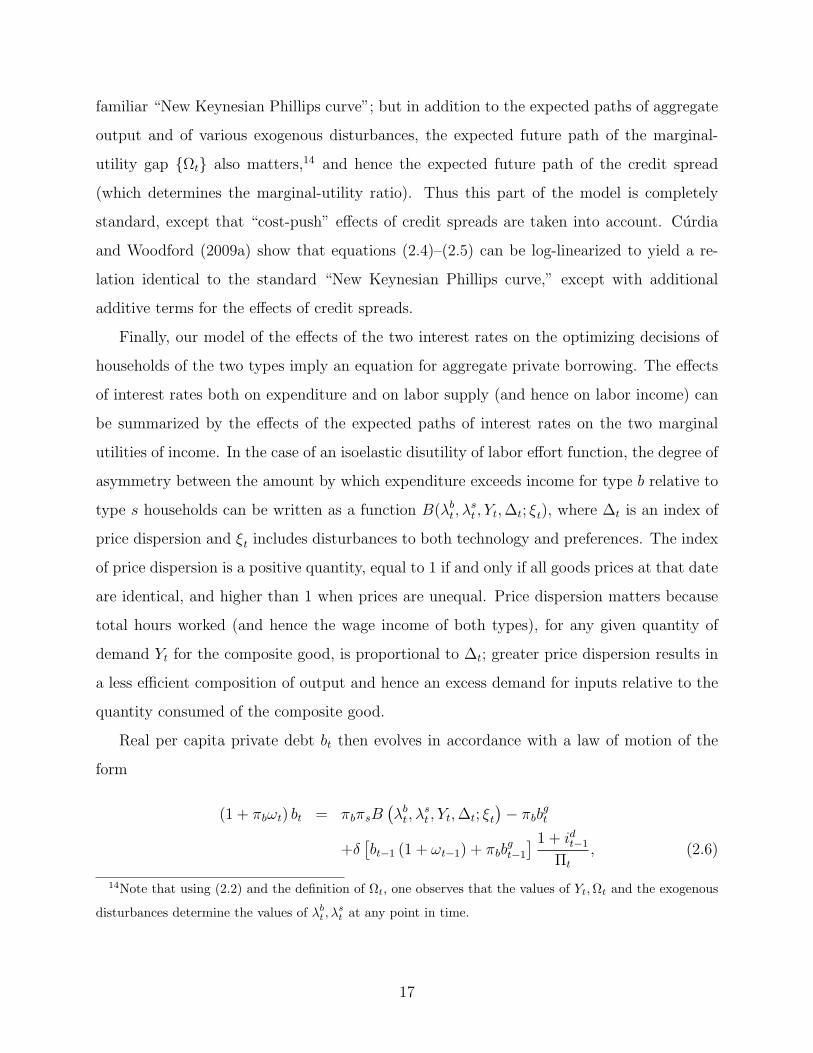
Real per capita private debt bt then evolves in accordance with a law of motion of the

form

(1 + πbωt) bt = πbπsB(λb

t , λst , Yt, ∆t; ξt

)− πbbgt

+δ[bt−1 (1 + ωt−1) + πbb

gt−1

] 1 + idt−1

Πt

, (2.6)

14Note that using (2.2) and the definition of Ωt, one observes that the values of Yt, Ωt and the exogenous

disturbances determine the values of λbt , λ

st at any point in time.

17

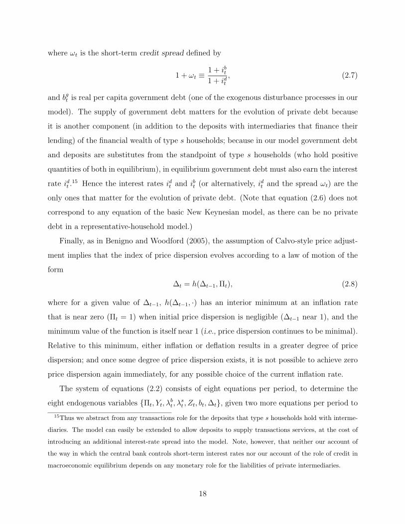
where ωt is the short-term credit spread defined by

1 + ωt ≡ 1 + ibt1 + idt

, (2.7)

and bgt is real per capita government debt (one of the exogenous disturbance processes in our

model). The supply of government debt matters for the evolution of private debt because

it is another component (in addition to the deposits with intermediaries that finance their

lending) of the financial wealth of type s households; because in our model government debt

and deposits are substitutes from the standpoint of type s households (who hold positive

quantities of both in equilibrium), in equilibrium government debt must also earn the interest

rate idt .15 Hence the interest rates idt and ibt (or alternatively, idt and the spread ωt) are the

only ones that matter for the evolution of private debt. (Note that equation (2.6) does not

correspond to any equation of the basic New Keynesian model, as there can be no private

debt in a representative-household model.)

Finally, as in Benigno and Woodford (2005), the assumption of Calvo-style price adjust-

ment implies that the index of price dispersion evolves according to a law of motion of the

form

∆t = h(∆t−1, Πt), (2.8)

where for a given value of ∆t−1, h(∆t−1, ·) has an interior minimum at an inflation rate

that is near zero (Πt = 1) when initial price dispersion is negligible (∆t−1 near 1), and the

minimum value of the function is itself near 1 (i.e., price dispersion continues to be minimal).

Relative to this minimum, either inflation or deflation results in a greater degree of price

dispersion; and once some degree of price dispersion exists, it is not possible to achieve zero

price dispersion again immediately, for any possible choice of the current inflation rate.

The system of equations (2.2) consists of eight equations per period, to determine the

eight endogenous variables Πt, Yt, λbt , λ

st , Zt, bt, ∆t, given two more equations per period to

15Thus we abstract from any transactions role for the deposits that type s households hold with interme-

diaries. The model can easily be extended to allow deposits to supply transactions services, at the cost of

introducing an additional interest-rate spread into the model. Note, however, that neither our account of

the way in which the central bank controls short-term interest rates nor our account of the role of credit in

macroeconomic equilibrium depends on any monetary role for the liabilities of private intermediaries.

18

determine the evolution of the interest rates idt , ibt (and hence of the credit spread). The

latter equations follow from the decisions of private intermediaries and of the central bank.

2.2 Financial Intermediaries

We assume an intermediary sector made up of identical, perfectly competitive firms. In-

termediaries take deposits, on which they promise to pay a riskless nominal return idt one

period later, and make one-period loans on which they demand a nominal interest rate of

ibt . An intermediary also chooses a quantity of reserves Mt to hold at the central bank, on

which it will receive a nominal interest yield of imt . Each intermediary takes as given all three

of these interest rates. We assume that arbitrage by intermediaries need not eliminate the

spread between ibt and idt , for either of two reasons. On the one hand, resources are used in

the process of loan origination; and on the other hand, intermediaries may be unable to tell

the difference between good borrowers (who will repay their loans the next period) and bad

borrowers (who will be able to disappear without having to repay), and as a consequence

have to charge a higher interest rate to good and bad borrowers alike.

We suppose that origination of good loans in real quantity Lt requires an intermediary

to also originate bad loans in quantity χt(Lt), where χ′t, χ′′t ≥ 0, and the function χt(L) may

shift from period to period for exogenous reasons. (While the intermediary is assumed to be

unable to discriminate between good and bad loans, it is able to predict the fraction of loans

that will be bad in the case of any given scale of lending activity on its part.) This scale of

operations also requires the intermediary to consume real resources Ξpt (Lt; mt) in the period

in which the loans are originated, where mt ≡ Mt/Pt, and Ξpt (L; m) is a convex function of

its two arguments, with ΞpLt ≥ 0, Ξp

mt ≤ 0, ΞpLmt ≤ 0. We further suppose that for any scale

of operations L, there exists a finite satiation level of reserve balances mt(L), defined as the

lowest value of m for which Ξpmt(L; m) = 0. (Our convexity and sign assumptions then imply

that Ξpmt(L; m) = 0 for all m ≥ mt(L).) We assume the existence of a finite satiation level of

reserves in order for an equilibrium to be possible in which the policy rate is driven to zero,

a situation of considerable practical relevance at present that raises interesting theoretical

issues.

Given an intermediary’s choice of its scale of lending operations Lt and reserve balances

19

mt to hold, we assume that it acquires real deposits dt in the maximum quantity that it

can repay (with interest at the competitive rate) from the anticipated returns on its assets

(taking into account the anticipated losses on bad loans). Thus it chooses dt such that

(1 + idt )dt = (1 + ibt)Lt + (1 + imt )mt.

The deposits that it does not use to finance either loans or the acquisition of reserve balances,

dt −mt − Lt − χt(Lt)− Ξpt (Lt; mt),

are distributed as earnings to its shareholders. The intermediary chooses Lt and mt each

period so as to maximize these earnings, given idt , ibt , i

mt . This implies that Lt and mt must

satisfy the first-order conditions

ΞpLt(Lt; mt) + χLt(Lt) = ωt ≡ ibt − idt

1 + idt, (2.9)

−Ξpmt(Lt; mt) = δm

t ≡ idt − imt1 + idt

. (2.10)

Equation (2.9) can be viewed as determining the equilibrium credit spread ωt as a function

ωt(Lt; mt) of the aggregate volume of private credit and the real supply of reserves. As

indicated above, a positive credit spread exists in equilibrium to the extent that Ξpt (L; m),

χt(L), or both are increasing in L. Equation (2.10) similarly indicates how the equilibrium

differential δmt between the interest paid on deposits and that paid on reserves at the central

bank is determined by the same two aggregate quantities.

In addition to these two equilibrium conditions that determine the two interest-rate

spreads in the model, the absolute level of (real) interest rates must be such as to equate the

supply and demand for credit. Market-clearing in the credit market requires that

bt = Lt + Lcbt , (2.11)

where Lcbt represents real lending to the private sector by the central bank, as discussed

next. Equations (2.9)–(2.11) then provide three more equilibrium conditions per period, to

determine the three additional endogenous variables ıdt , ibt , Lt along with those discussed in

the previous section, given paths (or rules for the determination of) the central-bank policy

variables Mt, imt , Lcb

t .

20

2.3 Dimensions of Central-Bank Policy

In our model, the central bank’s liabilities consist of the reserves Mt (which also constitute

the monetary base in our simple model), on which it pays interest at the rate imt . These

liabilities in turn fund the central bank’s holdings of government debt, and any lending by

the central bank to type b households. We let Lcbt denote the real quantity of lending by

the central bank to the private sector; the central bank’s holdings of government debt are

then given by the residual mt − Lcbt . We can treat mt (or Mt) and Lcb

t as the bank’s choice

variables, subject to the constraints

0 ≤ Lcbt ≤ mt. (2.12)

It is also necessary that the central bank’s choices of these two variables satisfy the bound

mt < Lcbt + bg

t ,

where bgt is the total outstanding real public debt, so that a positive quantity of public debt

remains in the portfolios of households. In the calculations below, however, we shall assume

that this last constraint is never binding. (We confirm this in our numerical examples.)

We assume that central-bank extension of credit other than through open-market pur-

chases of Treasury securities consumes real resources, just as in the case of private inter-

mediaries, and represent this resource cost by a function Ξcb(Lcbt ), that is increasing and

at least weakly convex, with Ξcb′(0) > 0, as is discussed further in section 4. The central

bank has one further independent choice to make each period, which is the rate of interest

imt to pay on reserves. We assume that if the central bank lends to the private sector, it

simply chooses the amount that it is willing to lend and auctions these funds, so that in

equilibrium it charges the same interest rate ibt on its lending that private intermediaries do;

this is therefore not an additional choice variable for the central bank. Similarly, the central

bank receives the market-determined yield idt on its holdings of government debt.

The interest rate idt at which intermediaries are able to fund themselves is determined

each period by the joint inequalities

mt ≥ mdt (Lt, δ

mt ), (2.13)

21

δmt ≥ 0, (2.14)

together with the “complementary slackness” condition that at least one of (2.13) and (2.14)

must hold with equality each period. Here mdt (L, δm) is the demand for reserves defined by

(2.10), and defined to equal the satiation level mt(L) in the case that δm = 0. (Condition

(2.13) may hold only as an inequality, as intermediaries will be willing to hold reserves

beyond the satiation level as long as the opportunity cost δmt is zero.) We identify the rate idt

at which intermediaries fund themselves with the central bank’s policy rate (e.g., the federal

funds rate, in the case of the US).

The central bank can influence the policy rate through two channels, its control of the

supply of reserves and its control of the interest rate paid on them. By varying mt, the central

bank can change the equilibrium differential δmt , determined as the solution to (2.13)–(2.14).

And by varying imt , it can change the level of the policy rate idt that corresponds to a

given differential. Through appropriate adjustment on both margins, the central bank can

control idt and imt separately (subject to the constraint that imt cannot exceed idt ). We also

assume that for institutional reasons, it is not possible for the central bank to pay a negative

interest rate on reserves. (We may suppose that intermediaries have the option of holding

currency, earning zero interest, as a substitute for reserves, and that the second argument

of the resource cost function Ξpt (b; m) is actually the sum of reserve balances at the central

bank plus vault cash.) Hence the central bank’s choice of these variables is subject to the

constraints

0 ≤ imt ≤ idt . (2.15)

There are thus three independent dimensions along which central-bank policy can be

varied in our model: variation in the quantity of reserves Mt that are supplied; variation in

the interest rate imt paid on those reserves; and variation in the breakdown of central-bank

assets between government debt and lending Lcbt to the private sector. Alternatively, we can

specify the three independent dimensions as interest-rate policy, the central bank’s choice of

an operating target for the policy rate idt ; reserve-supply policy, the choice of Mt, which in

turn implies a unique rate of interest that must be paid on reserves in order for the reserve-

supply policy to be consistent with the bank’s target for the policy rate;16 and credit policy,

16We might choose to call the second dimension variation in the interest rate paid on reserves, which

22

the central bank’s choice of the quantity of funds Lcbt to lend to the private sector.17

We prefer this latter identification of the three dimensions of policy because in this

case our first dimension (interest-rate policy) corresponds to the sole dimension of policy

emphasized in many conventional analyses of optimal monetary policy, while the other two

dimensions are additional dimensions of policy introduced by our extension of the basic

New Keynesian model.18 Changes in central-bank policy along each of these dimensions

has consequences for the bank’s cash flow, but we abstract from any constraint on the joint

choice of the three variables associated with cash-flow concerns. (We assume that seignorage

revenues are simply turned over to the Treasury, where their only effect is to change the size

of lump-sum transfers to the households.)

Given that central-bank policy can be independently varied along each of these three

dimensions, we can independently discuss the criteria for policy to be optimal along each

would correspond to something that the Board of Governors makes an explicit decision about under current

US institutional arrangements, as is also true at most other central banks. But description of the second

dimension of policy as “reserve-supply policy” allows us to address the question of the value of “quantitative

easing” under this heading as well.17Here we only consider the kind of credit policy that involves direct lending by the central bank to ultimate

borrowers, or (equivalently, in our model, since the loan market is competitive) targeted asset purchases.

Thus our “credit policy” is intended to represent, in a stylized way, the kind of programs that became an

important part of Fed policy after September 2008, such as the Commercial Paper Funding Facility mentioned

in section 1, or the Fed’s purchases of mortgage-backed securities. We do not take up the separate question of

what might be accomplished by central-bank lending to intermediaries rather than to ultimate borrowers, as

under the “liquidity facilities” that played such an important role in the Fed’s response to the financial crisis

up until September 2008. In our model, central-bank lending to intermediaries can also be effective; and as

with our analysis of credit policy below, the welfare consequences of such intervention will depend crucially

on whether financial disruptions involve increases in the real resource costs of private intermediation or not.

Other analyses that distinguish the effects of these two types of credit policy include Reis (2009) and Gertler

and Kiyotaki (2010).18Goodfriend (2009) similarly describes central-bank policy as involving three independent dimensions,

corresponding to our first three dimensions, and calls the first of those dimensions (the quantity of reserves,

or base money) “monetary policy.” We believe that this does not correspond to standard usage of the term

“monetary policy,” since the traditional focus of FOMC deliberations about monetary policy has been the

choice of an operating target for the policy rate, as is generally the case at other central banks as well. Reis

(2009) also distinguishes among the three dimensions of policy in terms similar to ours.

23

dimension. Here we restrict our analysis to the two “unconventional” dimensions of pol-

icy, reserve-supply policy and credit policy. The consequences of heterogeneity and credit

frictions for interest-rate policy (i.e., conventional monetary policy) are addressed in Curdia

and Woodford (2009a, 2009b). Of course, we have to make some assumption about interest-

rate policy when considering adjustments of policy along the other two dimensions; in some

of the analysis reported below, we assume that interest-rate policy is optimal (despite not

seeking here to characterize optimal interest-rate policy), while in other places we assume

a simple conventional specification for interest-rate policy (a “Taylor rule”). It is also true

that the changes in reserve-supply policy and credit policy have consequences for optimal

interest-rate policy; but these are not the concern of the present study, except to the extent

that they influence the optimal use of the unconventional policies themselves.

2.4 The Welfare Objective

In considering optimal policy, we take the objective of policy to be the maximization of

average expected utility. Thus we can express the objective as maximization of

Et0

∞∑t=t0

βt−t0Ut (2.16)

where the welfare contribution Ut each period weights the period utility of each of the two

types by their respective population fractions at each point in time. As shown in Curdia

and Woodford (2009a),19 this can be written as

Ut = U(Yt, Ωt, Ξt, ∆t; ξt), (2.17)

where Ωt is again the marginal-utility gap, Ωt ≡ λbt/λ

st ; Ξt is total resources consumed in

financial intermediation (also including resources used by the central bank, to the extent

19Curdia and Woodford (2009a) analyze a special case of the present model, in which central-bank lending

and the role of central-bank liabilities in reducing the transactions costs of intermediaries are abstracted

from. However, the form of the welfare measure (2.17) depends only on the nature of the heterogeneity in

our model, and the assumed existence of a credit spread and of resources consumed by the intermediary

sector; the functions that determine how Ωt and Ξt are endogenously determined are irrelevant for this

calculation, and those are the only parts of the model that are generalized in this paper. Hence the form of

the welfare objective in terms of these variables remains the same.

24

that it lends to the private sector, as discussed further in sections 4 and 5); ∆t is the index

of price dispersion appearing in (2.6)–(2.8); and ξt is a vector of exogenous disturbances to

preferences, technology, and government purchases.

It may be useful to briefly explain why the arguments in (2.17) suffice, and the way

each of them affects welfare. In order to derive the period objective in (2.17), we sum the

utility of consumption and disutility of labor for the two types, weighting each type τ by

its population fraction πτ . The average utility of consumption is equal to∑

τ πτuτ (cτ

t ; ξt),

which depends on cbt , c

st , and exogenous shocks to preferences (i.e., to spending opportunities).

But it is possible to solve uniquely for cbt , c

st given values for Yt, Ωt, Ξt, and the exogenous

disturbances (including Gt), using (2.2) and the definition of Ωt; hence the arguments of

(2.17) suffice to determine this component of average utility. The total disutility of work can

be written as a product of factors

Λ(Ωt)v(Yt; ξt)∆t,

where v(Yt; ξt) would be the disutility of supplying quantity Yt of the composite good, if a

common quantity yt(j) = Yt were produced of each of the individual goods, and if the labor

effort involved in producing them were efficiently divided between households of the two

types;20 and Λ(Ωt) is a distortion factor that arises as a result of differing marginal utilities

of income of the two types (which means that their relative wages no longer correctly reflect

their relative marginal disutilities of work), leading to an inefficient division of equilibrium

work effort across the two types of households. Given these other two factors, the total

disutility of work is proportional to ∆t because greater price dispersion results in a less

efficient composition of the output that comprises a quantity Yt of the composite good.

(Note that except for the presence of the factor Λ(Ωt), the total disutility of work is the

same as in the representative household model.) Hence the arguments of (2.17) also suffice

for the calculation of this term, and so for the calculation of the period t contribution to

average utility.

From this discussion, it should be evident how each of the four endogenous variables in

(2.17) affects welfare. Given the values of the other variables, increasing Yt increases the

20Note that this disutility will depend both on the state of productivity and on preferences regarding labor

supply, both of which are elements of the vector ξt.

25

average utility of consumption but also the total disutility of work, as in the representative

household model. Under standard assumptions about preferences and technology, there is

diminishing marginal utility from consumption and increasing marginal disutility of work

as Yt increases, so that there should be an interior maximum for Ut as a function of Yt

(the location of which will depend on preferences, technology, government purchases, etc.).

And given the values of the other variables, Ut is monotonically decreasing in ∆t. Both

of these effects are similar to those in the representative household model, where Yt, ∆tare the only endogenous variables that matter for welfare.21 With heterogeneity and credit

frictions, additional variables become relevant as well. Given values of the other variables,

Ut is monotonically decreasing in both Ωt and Ξt. Average utility is reduced by an increase

in Ωt because both the efficiency of the allocation of total private expenditure across the two

types and the efficiency of the allocation of total work effort across the two types is reduced;

it is reduced by an increase in Ξt because, for given values of Yt and Gt, a higher value of Ξt

means less total private expenditure and hence lower values of both cbt and cs

t (given a value

for Ωt).

Other variables matter for welfare purely through their effects on the paths of these four

endogenous variables. For example, the level of real bank reserves matters in our model,

because of its effect on the resources Ξt consumed by financial intermediaries. Central-bank

credit policy can matter in our model as well, to the extent that it reduces credit spreads

and as a consequence the size of the equilibrium marginal-utility gap Ωt. We turn now to

an analysis of the optimal use of these additional dimensions of policy in the light of this

objective.

3 Reserve-Supply Policy

We shall first consider optimal policy with regard to the supply of reserves, taking as given

(for now) the way in which the central bank chooses its operating target for the policy rate idt ,

21Because the evolution of price dispersion is determined entirely by the path of inflation, as indicated by

(2.8), we can alternatively state that aggregate output and inflation are the only endogenous variables that

matter for welfare in the representative-household model.

26

and the state-contingent level of central-bank lending Lcbt to the private sector. Under fairly

weak assumptions, we obtain a very simple result: optimal policy requires that intermediaries

be satiated in reserves, i.e., that Mt/Pt ≥ ¯mt(Lt) at all times.

For levels of reserves below the satiation point, an increase in the supply of reserves has

two effects that are relevant for welfare: on the one hand, the resource cost of financial

intermediation Ξpt is reduced (for a given level of lending by the intermediary sector); and

on the other hand, the credit spread ωt is reduced (again, for a given level of lending) as

a consequence of (2.9). Each of these effects raises the value of the objective (2.16); note

that reductions in credit spreads increase welfare because of their effect on the path of the

marginal-utility gap Ωt.22 Hence an increase in the supply of reserves is unambiguously

desirable, in any period in which they remain below the satiation level.23Once reserves are at

or above the satiation level, however, further increases reduce neither the resource costs of

intermediaries nor equilibrium credit spreads (as in this case Ξpmt = Ξp

Lmt = 0), so that there

would be no further improvement in welfare. Hence policy is optimal along this dimension

if and only if Mt/Pt ≥ ¯mt(Lt) at all times,24 so that

Ξpmt(Lt; mt) = 0. (3.1)

This is just another example in which the familiar “Friedman Rule” for “the optimum

quantity of money” (Friedman, 1969) applies. Note, however, that our result has no con-

sequences for interest-rate policy. While the Friedman rule is sometimes taken to imply a

strong result about the optimal control of short-term nominal interest rates — namely, that

the nominal interest rate should equal zero at all times — the efficiency condition (3.1),

together with the equilibrium relation (2.10), implies only that the interest-rate differential

δmt should equal zero at all times. With zero interest on reserves, this would also require

22Log-linearization of equations (2.3) can be used to show that, up to this log-linear approximation, log

deviations of the marginal-utility gap should equal a forward-looking moving average of expected deviations

of the credit spread from its steady-state level; see Curdia and Woodford (2009a).23The discussion here assumes that the upper bound in (2.12) is not a binding constraint. But if that

constraint does bind, then an increase in the supply of reserves relaxes the constraint, and this too increases

welfare, so that the conclusion in the text is unchanged.24To be more precise, policy is optimal if and only if (3.1) is satisfied and the upper bound in (2.12) does

not bind. Both conditions will be satisfied by any quantity of reserves above some finite level.

27

that idt = 0 at all times; but given that the central bank is free to set any level of interest on

reserves consistent with (2.15), the efficiency condition (3.1) actually implies no restriction

upon either the average level of the degree of state-contingency of the central bank’s target

for the policy rate idt .

3.1 Is a Reserve Supply Target Needed?

Our result about the importance of ensuring an adequate supply of reserves might suggest

that the question of the correct target level of reserves at each point in time should receive

the same degree of attention at meetings of the FOMC as the question of the correct op-

erating target for the federal funds rate. But deliberations of that kind are not needed in

order to ensure fulfillment of the optimality criterion (3.1). For the efficiency condition can

alternatively be stated (using (2.10)) as requiring that idt = imt at all times. Reserves should

be supplied to the point at which the policy rate falls to the level of the interest rate paid on

reserves, or, in a formulation that is more to the point, interest should be paid on reserves

at the central bank’s target for the policy rate.

Given a rule for setting an operating target for idt (discussed in the next section), imt

should be chosen each period in accordance with the simple rule

imt = idt . (3.2)

When the central bank acts to implement its target for the policy rate through open-market

operations, it will automatically have to adjust the supply of reserves so as to satisfy (3.1).

But this does not require a central bank’s monetary policy committee (the FOMC in the

case of the US) to deliberate about an appropriate target for reserves at each meeting;

once the target for the policy rate is chosen (and the interest rate to be paid on reserves is

determined by that, through condition (3.2), the quantity of reserves that must be supplied

to implement the target can be determined by the bank staff in charge of carrying out the

necessary interventions (the trading desk at the New York Fed, in the case of the US), on

the basis of a more frequent monitoring of market conditions than is possible on the part of

the monetary policy committee.

One obvious way to ensure that the efficiency condition (3.2) is satisfied is to adopt a

28

routine practice of automatically paying interest on reserves at a rate that is tied to the

current operating target for the policy rate. This is already the practice of many central

banks outside the US. At some of those banks, the fixed spread between the target for the

policy rate and the rate paid on overnight balances at the central bank is quite small (for

example, 25 basis points in the case of the Bank of Canada); in the case of New Zealand, the

interest rate paid on overnight balances is the policy rate itself. There are possible arguments

(relating to considerations not reflected in our simple model) according to which the optimal

spread might be larger than zero, but it is likely in any event to be desirable to maintain a

constant small spread, rather than treating the question of the interest rate to be paid on

reserves as a separate, discretionary policy decision to be made at each meeting of the policy

committee. Apart from the efficiency gains modeled here, such a system should also help to

facilitate the central bank’s control of the policy rate (Goodfriend, 2002; Woodford, 2003,

chap. 1, sec. 3).

3.2 Is there a Role for “Quantitative Easing”?

While our analysis implies that it is desirable to ensure that the supply of reserves never falls

below a certain lower bound mt(Lt), it also implies that there is no benefit from supplying

reserves beyond that level. There is, however, one important exception to this assertion: it

can be desirable to supply reserves beyond the satiation level if this is necessary in order

to make the optimal quantity of central bank lending to the private sector Lcbt consistent

with (2.12). This qualification is important in thinking about the desirability of the massive

expansion in the supply of reserves by the Fed since September 2008, as shown in Figure 1.

As can be seen from Figure 2, the increase in reserves occurred only once the Fed decided to

expand the various newly-created liquidity and credit facilities beyond the scale that could

be financed simply by reducing its holdings of Treasury securities (as had been its policy

over the previous year).25

25Bernanke (2009) distinguishes between the Federal Reserve policy of “credit easing” and the type of

“quantitative easing” practiced by the Bank of Japan earlier in the decade, essentially on this ground.

Shiratsuka (2009) distinguishes between “pure credit easing” and “pure quantitative easing” in the way that

we have proposed, but argues that the actual “unconventional policies” of central banks, including both the

29

Some have argued, instead, that further expansion of the supply of reserves beyond the

level needed to bring the policy rate down to the level of interest paid on reserves is an

important additional tool of policy in its own right — one of particular value precisely when

a central bank is no longer able to further reduce its operating target for the policy rate,

owing to the zero lower bound (as at present in the US and many other countries). It is

sometimes proposed that when the zero lower bound is reached, it is desirable for a central

bank’s policy committee to shift from deliberations about an interest-rate target to a target

for the supply of bank reserves, as under the Bank of Japan’s policy of “quantitative easing”

during the period between March 2001 and March 2006.

Our model provides no support for the view that such a policy should be effective in

stimulating aggregate demand. Indeed, it is possible to state an irrelevance proposition for

quantitative easing in the context of our model. Let the three dimensions of central-bank

policy be described by functions that specify the operating target for the policy rate, the

supply of reserves, the interest rate to be paid on reserves, and the quantity of central-bank

credit as functions of macroeconomic conditions.

For the sake of concreteness, we may suppose that each of these variables is to be deter-

mined by a Taylor-type rule,

idt = φid(πt, Yt, Lt; ξt),

Mt/Pt = φm(πt, Yt, Lt; ξt),

imt = φim(πt, Yt, Lt; ξt),

Lcbt = φL(πt, Yt, Lt; ξt),

where the functions are such that constraints (2.12)–(2.15) are satisfied for all values of

the arguments. (Here the vector of exogenous disturbances ξt upon which the reaction

functions may depend includes the exogenous factors that shift the function Ξpt (L; m).)

Then our result is that given the three functions φid(·), φim(·), and φL(·), the set of pro-

cesses πt, Yt, Lt, bt, idt , i

bt , Ωt, ∆t that constitute possible rational expectations equilibria is

Bank of Japan in 2001-06 and the Federal Reserve during the current crisis, are mixtures of the two pure

types. Ueda (2009) similarly argues that many central banks represent mixed cases.

30

the same, independently of the choice of the function φm(·), as long as the specification of

φm(·) is consistent with the other three functions (in the sense that (2.12) and (2.13) are

necessarily satisfied, and that (2.13) holds with equality in all cases where (2.14) is a strict

inequality).26

Of course, the stipulation that φm(·) be consistent with the other functions uniquely

determines what the function must be for all values of the arguments for which the functions

id(·) and im(·) imply that δmt > 0. However the class of policies considered allows for an

arbitrary degree of expansion of reserves beyond the satiation level in the region where those

functions imply that δmt = 0, and in particular, for an arbitrary degree of quantitative easing

when the zero bound is reached (i.e., when idt = imt = 0). The class of policies considered

includes the popular proposal under which the quantity of excess reserves should depend on

the degree to which a standard Taylor rule (unconstrained by the zero bound) would call for

a negative policy rate. Our result implies that there should be no benefits from such policies.

Our result might seem to be contradicted by the analysis of Auerbach and Obstfeld (2004),

in which an open market operation that expands the money supply is found to stimulate real

activity even when the economy is at the zero bound at the time of the monetary expansion.

But their thought experiment does not correspond to pure quantitative easing of the kind

contemplated in the above proposition, because they specify monetary policy in terms of a

path for the money supply, and the policy change that they consider is one that permanently

increases the money supply, so that it remains higher after the economy has exited from the

“liquidity trap” in which the zero bound is temporarily binding. The contemplated policy

change is therefore not consistent with an unchanged reaction function φid(·) for the policy

rate, and the effects of the intervention can be understood to be the consequences of the

commitment to a different future interest-rate policy.

Our result only implies that quantitative easing should be irrelevant under two condi-

tions: that the increase in reserves finances an increase in central-bank holdings of Treasury

securities, rather than an increase in central-bank lending to the private sector; and that the

policy implies no change in the way that people should expect future interest-rate policy to

26This result generalizes the irrelevance result for quantitative easing in Eggertsson and Woodford (2003)

to a model with heterogeneity and credit frictions.

31

be conducted. Our model does allow for real effects of an increase in central-bank lending

Lcbt financed by an increase in the supply of reserves, in the case that private-sector financial

intermediation is inefficient;27 but the real effects of the increased central-bank lending in

that case are the same whether the lending is financed by an increase in the supply of reserves

or by a reduction in central-bank holdings of Treasury securities. Our model also allows for

real effects of an announcement that interest-rate policy in the future will be different, as in

the case where a central bank commits itself not to return immediately to its usual Taylor

rule as soon as the zero bound ceases to bind, but promises instead to maintain policy ac-

commodation for some time after it would become possible to comply with the Taylor rule

(as discussed in the next section). But such a promise (if credible and correctly understood

by the private sector) should increase output and prevent deflation to the same extent even

if it implies no change in policy during the period when the zero lower bound binds.

While our definition of quantitative easing may seem a narrow one, the policy of the Bank

of Japan during the period 2001-2006 fits our definition fairly closely. The BOJ’s policy

involved the adoption of a series of progressively higher quantitative targets for the supply

of reserves, and the aim of the policy was understood to be to increase the monetary base,

rather than to allow the BOJ to acquire any particular type of assets. The assets purchased

consisted primarily Japanese government securities and bills issued by commercial banks;

while there were also some more “unconventional” asset purchases under the quantitative

easing policy — direct purchases of asset-backed securities and of stocks — the size of these

operations was quite small relative to the total increase in the supply of reserves shown in

Figure 4.28 Finally, there was no suggestion that the targets of policy after the end of the

27This result differs from that obtained in Eggertsson and Woodford (2003), where changes in the compo-

sition of the assets on the central bank’s balance sheet are also shown to be irrelevant. That stronger result

depends on the assumption of a representative household as in the earlier paper, or alternatively, frictionless

financial intermediation, as discussed in section 1.28According to Bank of Japan statistics, these “unconventional” purchases had a value only slightly greater

than 2 trillion yen at their maximum, whereas the total increase in the monetary base during the quantitative

easing (QE) period was in excess of 45 trillion yen. For more detailed discussion of the different aspects of

the BOJ policy during the period, and an attempt to separate the effects of targeted asset purchases from

those of quantitative easing, see Ueda (2009). Shiratsuka (2009) provides additional information.

32

zero-interest-rate period would be any different than before; there was no commitment to

maintain the increased quantity of base money in circulation permanently, and indeed, once

it was judged time to end the zero-interest-rate policy, the supply of reserves was rapidly

contracted again, as also shown in Figure 4.

Our theory suggests that expansion of the supply of reserves under such circumstances

should have little effect on aggregate demand, and this seems to have been the case. For

example, as is also shown in Figure 4, despite an increase in the monetary base of 60 percent

during the first two years of the quantitative easing policy, and an eventual increase of nearly

75 percent, nominal GDP never increased at all (relative to its March 2001 level) during

the entire five years of the policy.29 Apart from the absence of the effects on aggregate

expenditure that simple quantity-theoretic reasoning would have predicted, there was also

little evidence of effects of the policy on longer-term interest rates (the channel through

which it might have been expected to ultimately influence aggregate expenditure). Those

studies of Japan’s experience with quantitative easing that find some reduction in longer-

term interest rates attribute this mainly to successful signalling by the BOJ of an intention

to maintain the zero-interest-rate policy, and find little effect on bond yields of the increase

in the supply of reserves itself (Okina and Shiratsuka, 2004; Oda and Ueda, 2007; Ugai,

2007; Ueda, 2009).30 Of course, it is perfectly consistent with our model that signals about

future interest-rate policy can be an effective channel through which a central bank can seek

to provide further monetary stimulus even when the current policy rate is constrained by

the zero lower bound.31

29As indicated in Figure 4, over the first two years of the quantitative easing policy, nominal GDP fell

by more than 4 percent, despite extremely rapid growth of base money. While nominal GDP recovered

thereafter, it remained below its 2001:Q1 level over the entire period until 2006:Q4, three quarters after the

official end of quantitative easing, by which time the monetary base had been reduced again by more than

20 percent. Moreover, even if the growth of nominal GDP after 2003:Q1 is regarded as a delayed effect of the

growth in the monetary base two years earlier, this delayed nominal GDP growth was quite modest relative

to the size of the expansion in base money.30Baba et al. (2006) find some effects of BOJ purchases of commercial paper on the spreads associated

with those particular types of paper. But this is really more evidence of the effectiveness of targeted asset

purchases than of effectiveness of quantitative easing as such. See also the discussion by Ueda (2009).31See Eggertsson and Woodford (2003) and Curdia and Woodford (2009b) for further discussion of the

33

4 Central-Bank Asset Purchases: “Treasuries Only”?

We turn now to another of our three independent dimensions of central-bank policy, namely,

adjustment of the composition of the asset side of the central bank’s balance sheet, taking

as given the overall size of the balance sheet (determined by the reserve-supply decision

discussed above). In this section, we take for granted that reserve-supply policy is being

conducted in the way recommended in the previous section, i.e., that the rate of interest on

reserves will satisfy (3.2) at all times. In this case, we can replace the function Ξpt (Lt; mt) by

Ξpt (Lt) ≡ Ξp

t (Lt; mt(Lt))

and the function ωt(Lt; mt), defined by the left-hand side of (2.9), by

ωt(Lt) ≡ ωt(Lt; mt(Lt)),

since there will be satiation in reserves at all times.32 Using these functions to specify the

equilibrium evolution of Ξpt and ωt as functions of the evolution of aggregate private credit,

we can then write the equilibrium conditions of the model without any reference to the

quantity of reserves or to the interest rate paid on reserves. We wish to consider alternative

possible state-contingent evolutions for central-bank lending Lcbt , under various maintained

assumptions about interest-rate policy (made explicit below).

According to the traditional doctrine of “Treasuries only,” the central bank should not

vary the composition of its balance sheet as a policy tool; instead, it should avoid both

balance-sheet risk and the danger of politicization by only holding (essentially riskless)

Treasury securities at all times, while varying the size of its balance sheet to achieve its

stabilization goals for the aggregate economy.33 And even apart from these prudential con-

cerns, if private financial markets can be relied upon to allocate capital efficiently, it is hard

to argue that there would be any substantial value to allowing the central bank this addi-

tional dimension of policy. Eggertsson and Woodford (2003) present a formal irrelevance

proposition in the context of a representative-household general-equilibrium model; in their

effectiveness of and ideal use of this aspect of policy.32Even if at some times mt exceeds mt(Lt), this will not affect the values of Ξp

t or ωt.33See Goodfriend (2009) for discussion of this view and a warning about the dangers of departing from it.

34

model, the assets purchased by the central bank have no consequences for the equilibrium

evolution of output, inflation or asset prices — and this is true regardless of whether the

central bank purchases long-term or short-term assets, nominal or real assets, riskless or

risky assets, and so on. And even in a model with heterogeneity of the kind considered here,

the composition of the central bank’s balance sheet would be irrelevant if we were to assume

frictionless private financial intermediation, since private intermediaries would be willing to

adjust their portfolios to perfectly offset any changes in the portfolio of the central bank, as

discussed in section 1.

This irrelevance result does not hold, however, in the presence of credit frictions of the

kind assumed in section 2. Here we illustrate the potential use of central-bank credit as

an instrument of stabilization policy in a numerical example. After establishing that credit

policy can be used for macroeconomic stabilization in principle, we then consider the subtler

question of whether it is desirable to do so.

4.1 Numerical Calibration

We shall illustrate our main points through an analysis of the quantitative effects of alter-

native types of purely financial disturbances in a calibrated model. The numerical values

for parameters used in our calculations are summarized in Table 1. They are essentially the

same as those used in the numerical analysis in Curdia and Woodford (2009a), where they

are discussed in greater detail. The one important difference is that here we calibrate the

model so that the steady-state real return on deposits (identified with the real federal funds

rates, for purposes of the empirical interpretation of the model) is 3.0 percent per annum. In

Curdia and Woodford (2009a), this rate is calibrated to be 4 percent per annum (1 percent

per quarter), for the sake of using a round number (when expressed as a quarterly rate). But

because we are interested in the consequences of the zero lower bound on the policy rate in

some of the calculations reported below, the question of how far the steady-state policy rate

is from the lower bound is of non-trivial import. Hence we have here adopted a value for

this target that is closer to the average historical level of the real federal funds rate. Several

of the numbers in Table 1 are also slightly different from those reported in the appendix

to Curdia and Woodford (2009a), but all of these are consequences of the change in the

35

calibration target for the steady-state real policy rate, given unchanged numerical values for

the other calibration targets.

Our numerical analysis requires the introduction of functional forms for preferences, pro-

duction technology, and the functions that define the financial frictions. The utility from

expenditure is assumed to be of the form

uτ (c; ξt) ≡c1−σ−1

τ(Cτ

t

)σ−1τ

1− σ−1τ

,

for τ = b, s, where for each type, στ > 0 would be the intertemporal elasticity of substitution

of expenditure if one’s type were expected to remain unchanged, and Cτt is an exogenous

type-specific disturbance, indicating variation in aggregate spending opportunities. The

quantity c is a Dixit-Stiglitz aggregate of the household’s purchases of the various individual

goods, with elasticity of substitution θ > 1, assumed to be the same for households of both

types.34 The disutility of work is assumed to be of the form

vτ (h; ξt) ≡ψτ

1 + νh1+νH−ν

t ,

for τ = b, s, where ν > 0 is the inverse of the Frisch elasticity of labor supply for both types,

and Ht is an exogenous disturbance, also common to both types. (Note that the disutility

of work is assumed to be the same for both types, except for the multiplicative factors ψτ ,

that differ across types so as to imply identical steady-state labor supplies for the two types,

despite their differing steady-state marginal utilities of income.) The production technology

for each good j is assumed to be of the form

yt(j) = Atht(j)1/φ,

where φ > 1 indicates the degree of diminishing returns, and At is an exogenous productivity

factor, common to all goods.

Many of the model’s parameters are also parameters of the basic New Keynesian model,

and in the case of these parameters we assume similar numerical values as in the numerical

34The government is also assumed to purchase an exogenous quantity of the composite good, defined using

the same aggregator, so that the government’s elasticity of substitution among individual goods is also equal

to θ. This makes the elasticity of each firm’s demand curve independent of the composition of demand.

36

Table 1: Numerical parameter values used.

πb 0.5 sb 0.798 (θ − 1)−1 0.15 τ 0.2

δ 0.975 ss 0.602 φ−1 0.75 Ξ/Y 0.0003

β 0.990 σb 13.6 α 0.66 χ/L 0

ν 0.105 σs 2.72 bg/Y 0 1 + ω (1.02)1/4

hb/hs 1 λb/λ

s1.22 b/Y 3.2 η 51.6

analysis of that model in Woodford (2003, Table 5.1.), which in turn are based on the

empirical model of Rotemberg and Woodford (1997). Specifically, the values assumed for

ν, θ, and φ in Table 1 are the same as in Rotemberg and Woodford, and the average of the

elasticities στ is chosen so as to imply the same interest-elasticity of aggregate expenditure

as in Rotemberg and Woodford.35The value assumed for α, the fraction of goods prices that

remain unchanged from one quarter to the next, is also the same as in Rotemberg and

Woodford. The value assumed for β is also the same (to three decimal places) as the one

used by Rotemberg and Woodford, though for a different reason: the value reported in the

table is required by our calibration target for the steady-state real policy rate, discussed

above.36

The new parameters that are needed for the present model are those relating to hetero-

geneity or to the specification of the credit frictions. The parameters relating to heterogeneity

are the fraction πb of households that are borrowers, the degree of persistence δ of a house-

hold’s “type”, the steady-state expenditure level of borrowers relative to savers, and the

interest-elasticity of expenditure of borrowers relative to that of savers, σb/σs.37

35To be precise, these are chosen so that the coefficient σ defined in the Appendix has the same value as

the coefficient denoted σ in Table 5.1 of Woodford (2003).36Our calibration target for the steady-state real policy rate is slightly lower than the one assumed by

Rotemberg and Woodford, but the credit frictions in our model require a rate of time preference that is

slightly higher than the steady-state real policy rate, unlike the model of Rotemberg and Woodford; and the

consequences of these two changes for the assumed value of β essentially cancel one another.37Another new parameter that matters as a consequence of heterogeneity is the steady-state level of

government debt relative to GDP, bg/Y ; here we assume that bg = 0.

37

In the calculations reported here, we assume that πb = πs = 0.5, so that there are an

equal number of borrowers and savers. We assume that δ = 0.975, so that the expected

time until a household has access to the insurance agency (and its type is drawn again) is 10

years. This means that the expected path of the spread between lending and deposit rates

for 10 years or so into the future affects current spending decisions, but that expectations

regarding the spread several decades in the future are nearly irrelevant.

We calibrate the model so that private expenditure is 0.7 of total output in steady state,

and furthermore calibrate the degree of heterogeneity in the steady-state expenditure of the

two types so that the implied steady-state debt b is equal to 80 percent of annual steady-state

output.38 This value matches the median ratio of private (non-financial, non-government,

non-mortgage) debt to GDP over the period 1986-2008.39 This requires the values of sb and

ss shown in the table, where sτ ≡ cτ/Y is the steady-state expenditure share for each type

τ (using bars to denote the steady-state values of variables).

We assume an average intertemporal elasticity of substitution for the two types that is

the same as that of the representative household in the model of Rotemberg and Woodford

(1997), as mentioned above, and determine the individual values of στ for the two types

on the assumption that σb/σs is equal to 5. This is an arbitrary choice, though the fact

that borrowers are assumed to have a greater willingness to substitute intertemporally is

important, as this results in the prediction that an exogenous tightening of monetary policy

(a positive intercept shift added to (4.2)) results in a reduction in the equilibrium volume of

credit bt (see Curdia and Woodford, 2009a). This is consistent with the VAR evidence on

the effects of an identified monetary policy shock presented in Lown and Morgan (1992).40

It is also necessary to specify the unperturbed values of the functions ω(b) and Ξ(b)

38In our quarterly model, this means that b/Y = 3.2.39We exclude mortgage debt when calibrating the degree of heterogeneity of preferences in our model,

since mortgage debt is incurred in order to acquire an asset, rather than to consume current produced goods

in excess of current income.40It is also consistent with the evidence in Den Haan et al. (2004) for the effects of a monetary shock on

consumer credit, though commercial and industrial loans are shown to rise. The result for C&I loans may

reflect substitution of firms toward bank credit owing to decreased availability of other sources of credit,

rather than an actual increase in borrowing; see Bernanke and Gertler (1995) on this point.

38

that describe the financial frictions, in addition to making clear what kinds of random

perturbations of these functions we wish to consider when analyzing the effects of “financial

shocks.” In the absence of shocks, we assume that χt(L) = 0, so that all loans are expected

to be repaid, and the credit spread is due purely to the resource costs of intermediation.

We assume an intermediation technology such that when intermediaries hold reserves at or

above the satiation level (as occurs in equilibrium under an optimal reserve-supply policy,

assumed in all of the numerical exercises reported in this section)

Ξp(L) = ΞpLη (4.1)

in the absence of shocks. We assume that η > 1, so that the marginal cost of intermediation

is increasing; this corresponds to the idea of a finite lending capacity at a given point in

time, due to scarce factors such as intermediary capital and expertise that are here treated

as exogenous.41

In the numerical results reported here, we assume more specifically a value of η that

implies that a one percent increase in private lending implies an increase in the marginal

cost of intermediation, and hence in the equilibrium credit spread, of one percentage point

(per annum). This implies fairly inelastic credit supply by the private sector, but we believe

that this is the case of greatest interest for the exercises here, both because private credit

supply is often asserted to be quite inelastic during financial crises, and because this is in any

event the assumption most favorable to a potential role for central-bank credit policy, as in

this case a substitution of central-bank lending for private lending to even a modest degree

can lower the marginal cost of private lending and hence the equilibrium credit spread.42

We are interested in biasing our results in this direction, not to pre-judge the desirability

of central-bank lending, but because our results show in any event that the justification for

41The assumption that η > 1 also allows our model to match the prediction of VAR estimates that an

unexpected tightening of monetary policy is associated with a slight reduction in credit spreads (see, e.g.,

Lown and Morgan, 2002, and Gerali et al., 2008). See Curdia and Woodford (2009a) for comparison with a

model with a linear resource cost function.42In the case that the private intermediary sector has a constant marginal cost, rather than one increasing

with the volume of private lending, then central-bank lending will reduce the equilibrium credit spread only

to the extent that it completely replaces private lending, by lending at a rate that is too low to be profitable

for private intermediaries at any positive scale of operation.

39

active credit policy is often fairly modest, even in the case of financial disturbances that

increase credit spreads by a significant amount. It is most interesting to observe that this

is true even under the assumption of quite a large value for η; in the case of a more modest

value of η, then both the shadow value of allowing active credit policy (relaxing the constraint

that Lcbt = 0) and the optimal scale of central-bank lending in response to shocks will in all

cases be substantially smaller than the values reported below.

Finally, we specify the unperturbed value of Ξp so that the steady-state credit spread

ω equal to 2.0 percentage points per annum, following Mehra et al., (2008). Combined

with our assumption that “types” persist for 10 years on average, this implies a steady-

state “marginal-utility gap” Ω ≡ λb/λ

s= 1.22, so that there would be a non-trivial welfare

gain from transferring further resources from savers to borrowers. Because of the degree

of convexity assumed for the intermediation technology, this corresponds to a steady-state

resource cost of financial intermediation Ξ that is much smaller than 2 percent per year of the

steady-state level of private lending, as shown in Table 1;43 hence in our parameterization,

the credit spread represents mainly rents earned by private intermediaries, owing to the

scarcity of whatever factor allows only particular firms to engage in this activity.

4.2 Credit Policy and Stabilization

We first demonstrate that according to our model, central-bank credit policy can in principle

be a highly effective tool for macroeconomic stabilization. In particular, it can be used to

offset at least some of the effects of a “purely financial” disturbance, that shifts the relation

ωt(L), by shifting the relationship that would otherwise exist between private borrowing bt

and private lending Lt, so that the relationship between ωt and bt need not change. In the

numerical examples considered in Figures 5 and 6, we assume that χt(L) = χtL, and consider

the effects of an exogenous increase in the factor χt.44 Thus we assume that the fraction

of loans that are not repaid is independent of the volume of lending, but that it varies over

43The value for Ξ reported in the table represents the steady-state value of Ξpt , as we assume no central-

bank lending to the private sector in the steady state: Lcb = 0.44This is the type of disturbance that is called an “additive χ” shock in the next section.

40

time for exogenous reasons. We assume that

χt = chi0 ρt

for all t ≥ 0, where χ0 > 0 determines the size of the shock, and in our numerical examples

we assume that ρ = 0.9.

Let us suppose that interest-rate policy is specified by a “Taylor rule” of the form

idt = maxrd + φππt + φyYt, 0, (4.2)

where our specification assumes that the central bank’s operating target must at all times

respect the zero lower bound on short-term nominal interest rates. Here πt ≡ log Πt is the

inflation rate, Yt ≡ log(Yt/Y ), and rd is the steady-state real policy rate,45 so that the policy

rule is consistent with the zero-inflation steady state (discussed above) in the absence of

disturbances. In the numerical results shown in Figure 5 and subsequently, the response

coefficients are assigned the values φπ = 2, φy = 1/4, in rough accordance with estimates of

US monetary policy in recent decades.46

As a simple example of endogenous credit policy, let us suppose that the central bank’s

lending to the private sector (or purchases of illiquid assets) is given by a rule of the form

Lcbt = −γ(Lt − L), (4.3)

where L is the level of private lending in the zero-inflation steady state with zero central-

bank credit, and 0 ≤ γ ≤ 1 is a coefficient indicating the degree to which the central bank

increases its lending to the private sector to offset an observed decrease in private lending.47

The rule is specified so that the central bank adheres to a policy of “Treasuries only” in

45As explained above, we calibrate the model so that 1 + rd = (1.03)1/4.46These are the baseline parameter values used in the numerical analysis of the representative-household

New Keynesian model in Woodford (2003, chap. 4). We use these parameter values in our analysis in

Curdia and Woodford (2009a) of the model’s implications for the effects of disturbances when monetary

policy follows a Taylor rule, in order to allow direct comparison with the results shown in Woodford (2003)

for the basic New Keynesian model.47Of course, the decrease in private lending in equilibrium will not be independent of the central bank’s

intervention; as Figures 5 and 6 show, for a given size of disturbance, more lending by the central bank

results in a greater contraction of private lending.

41

the steady state, and so central-bank credit policy is eventually phased out again following

the disturbance. In the case that γ = 0, it adheres to “Treasuries only” even in response

to the financial disturbance; in the opposite limiting case, in which γ = 1, the central bank

uses credit policy so aggressively as to completely stabilize private borrowing bt at the level

b = L.48

Figure 5 plots the impulse responses of several endogenous variables to a disturbance

of the kind proposed, for each of several different values of γ. In the figure, a value of χ0

is assumed that increases the value of ω0(L) by 4 percentage points per annum. 49 In

the case of no credit policy (γ = 0), and an interest-rate policy that does not respond to

the disturbance except to the extent that it affects inflation or output, such a disturbance

contracts real activity and creates deflation, resulting in an immediate cut in the policy

rate.50 The reduction in the policy rate is not as large as the increase in the credit spread

ωt, so the interest rate faced by borrowers increases; given that expected inflation falls at the

same time, the increase in the real rate faced by borrowers is even greater. In addition to

the distortions implied by the effects of the disturbance on aggregate output and inflation,

there is also a substantial distortion of the composition of expenditure, as type b expenditure

falls sharply while type s expenditure actually increases; since by hypothesis, there has been

no change in the marginal utility of each type of expenditure, this shift in composition is

inefficient.

48In order to determine the general-equilibrium effects of this policy, it is also necessary to make an

assumption about the resources (if any) consumed by the central bank’s lending operations. For reasons dis-

cussed in the next section, we do assume that central-bank lending to the private sector consumes resources,

though central-bank purchases of Treasuries involve no costs. The cost parameter Ξcb is set in the same way

as in Figure xx, discussed below. However, the precise value of this parameter has very little effect on the

responses shown in Figure 5.49Even in the absence of active credit policy, this increases the equilibrium credit spread by less than 3

percentage points, because of the endogenous response of the equilibrium credit spread to the reduction in

private lending.50Note that in the case of a disturbance of this size, the policy rate is cut by about two percentage points,

but not so far as to cause the zero lower bound to become an issue. Hence for any small enough value of χ0,

the responses will look like those in Figure 5, with the size of all responses scaled in proportion to the value

of χ0.

42

The figure shows that active credit policy can mitigate each of the effects of the distur-

bance just mentioned. If γ > 0, private borrowing bt falls by less in equilibrium, while at the

same time the credit spread ωt increases by less (since private lending Lt actually falls more

if the central bank substitutes for private lenders). As a consequence, the marginal-utility

gap Ωt increases less, there is less distortion of the composition of private expenditure, there

is less contraction of aggregate expenditure and of output, and there is less deflation. More-

over, there is less need for interest-rate cuts to head off the output contraction and deflation:

output and inflation fall less even though the policy rate is cut less aggressively. In the

limiting case in which γ = 1, there is virtually no change in any of the endogenous variables,

except that Lt is falling and Lcbt is increasing (with total lending unchanged).51 In this case,

credit policy succeeds to a large extent in eliminating the instability that would otherwise

result from the financial disturbance; moreover, it virtually eliminates the need for a cut in

the policy rate.

While it is clear from this example that credit policy can be used for stabilization pur-

poses, one might still wonder whether it is needed: could not interest-rate policy already

accomplish as much, if we allow interest-rate policy to respond to the shock, rather than

assuming mechanical compliance with a simple Taylor rule? While modification of the as-

sumed interest-rate policy (for example, assuming a “spread-adjusted Taylor rule” of the

kind considered in Curdia and Woodford, 2010, under which the intercept of the Taylor rule

is reduced in proportion to any increase in the credit spread) can indeed mitigate the effects

of the disturbance that are shown for the case γ = 0 in the figure, it would not reduce them

to the extent that the credit policy with γ = 1 is able to. The reason is that the disturbance

shifts up the schedule ωt(L); in the absence of central-bank lending, this means that either

the credit spread must increase (which will distort the composition of expenditure, regardless

of the absolute level of interest rates) or borrowing must decrease (which would also require

a reduction of the relative spending of borrowers), or both. Thus while a large enough cut in

51It is not quite true that there is no change in the various endogenous variables, because the shift from

private lending to central-bank lending slightly increases the resources consumed in financial intermediation.

However, under our parameterization, this resource use is small enough that the effects on both aggregate

output and private expenditure are similar to those that would occur in the absence of the disturbance.

43

the policy rate can prevent output from declining, this policy will not eliminate the distortion

of the composition of expenditure.

The inadequacy of interest-rate policy alone is even more obvious in the case of a financial

disturbance large enough to cause the zero lower bound on the policy rate to bind. Figure 6

plots impulse responses to the same kind of disturbance as in Figure 5, but when the shock

is assumed to be three times as large.52 In this case, under the γ = 0 policy, the contraction

of output and reduction in inflation are sufficiently extreme that the zero lower bound on the

policy rate binds, assuming an interest-rate policy that is again determined by the Taylor

rule (4.2). The effects of the disturbance in the absence of credit policy are slightly more

than three times as great as those shown in Figure 5, owing to the binding zero lower bound.

But even more importantly, it is obvious in this case that it would not be possible to avoid

those effects simply by assuming an even more aggressive reduction in the policy rate than

that called for by the Taylor rule; for the zero lower bound would in any event prevent deeper

interest-rate cuts at the time of the shock. Yet once again, a sufficiently aggressive credit

policy can almost completely insulate aggregate output, both types of private expenditure,

and inflation from any effects of the disturbance.

4.3 Credit Policy and Welfare

We have seen from Figures 5 and 6 that credit policy can be used to stabilize the economy,

most notably in response to purely financial disturbances that shift the ωt(L) schedule. But is

it desirable to do so, and to what extent? Our model can also be used to consider the optimal

use of this additional dimension of policy, if we are willing to suppose that the prudential

arguments against the central bank’s involvement in the allocation of credit should not be

determinative, at least in the case of sufficiently severe financial disruptions. In our model, an

increase in Lcbt can improve welfare on two grounds: for a given volume of private borrowing

bt, an increase in Lcbt allows the volume of private lending Lt to fall, which should reduce

both the resources Ξpt consumed by the intermediary sector and the equilibrium credit spread

ωt (due to equilibrium relation (2.9)). Under plausible conditions, our model implies both

52That is, ω0(L) is increased by 12 percentage points per annum.

44

a positive shadow value ϕΞ,t of reductions in Ξt (the Lagrange multiplier associated with

the resource constraint (2.2)) and a positive shadow value ϕω,t of reductions in ωt; hence an

increase in Lcbt should be desirable on both grounds.

In the absence of any assumed cost of central-bank credit policy, one can easily obtain

the result that it is always optimal for the central bank to lend in amount sufficient to

allow an equilibrium with Lt = 0, i.e., the central bank should substitute for private credit

markets altogether. Of course, we do not regard this as a realistic conclusion. As a simple

way of introducing into our calculations the fact that the central bank is unlikely to have a

comparative advantage at the activity of credit allocation under normal circumstances, we

assume that central-bank lending consumes real resources in a quantity Ξcb(Lcbt ), by analogy

with our assumption that real resources Ξpt are consumed by private intermediaries. The

function Ξcb(L) is assumed to be increasing and at least weakly convex; in particular, we

assume that Ξcb′(0) > 0, so that there is a positive marginal resource cost of this activity, even

when the central bank starts from a balance sheet made up entirely of Treasury securities.

The first-order conditions for optimal choice of Lcbt then become:

ϕΞ,t[Ξp′t (bt − Lcb

t )− Ξcb′(Lcbt )] + ϕω,t[Ξ

p′′t (bt − Lcb

t ) + χ′′t (bt − Lcbt )] ≤ 0, (4.4)

Lcbt ≥ 0, (4.5)

together with the complementary slackness condition that at least one of conditions (4.4) or

(4.5) must hold with equality in each period. (Here the first expression in square brackets

in (4.4) is the partial derivative of Ξt with respect to Lcbt , holding constant the value of total

borrowing bt, while the second expression in square brackets is the partial derivative of ωt

with respect to Lcbt under the same assumption.)

A “Treasuries only” policy is optimal in the event of a corner solution, in which (4.4) is an

inequality, as will be the case if Ξcb′(0) is large enough. In our view, it is most reasonable to

calibrate the model so that this is true in steady state. Then not only will the optimal policy

involve “Treasuries only” in the steady state, but (assuming that the inequality is strict at

the steady state) this will continue to be true in the case of any stochastic disturbances that

are small enough. However, it will remain possible for the optimal policy to require Lcbt > 0

in the case of certain large enough disturbances. This is especially likely to be true in the

45

case of large enough disruptions of the financial sector, of a type that increase the marginal

resource cost of private intermediation (the value of Ξp′) and/or the degree to which increases

in private credit require a larger credit spread (the value of ω′).

However, not all “purely financial” disturbances — by which we mean exogenous shifts

in the functions Ξpt (L) or χt(L) of a type that increase the equilibrium credit spread ωt(L)

for a given volume of private credit — are equally likely to justify an active central-bank

credit policy on the grounds just mentioned. In fact, the optimal credit policy response to a

given shift in the function ωt(L) depends greatly on the source of the shift.53 To illustrate

this, we consider the quantitative effects of alternative types of purely financial disturbances

in our calibrated model.

4.4 The Value of Relaxing the “Treasuries Only” Restriction

We first assume that a strict policy of “Treasuries only” is maintained, but seek to determine

the shadow value of relaxing this constraint, i.e., the marginal increase in the value of the

welfare objective (2.16) that is achieved by a marginal increase in Lcbt above zero in some

period. This shadow value is given by the left-hand side of (4.4); a positive value would imply

that welfare is increased by allowing Lcbt to be positive.54 Since the shadow value is obviously

reduced if we assume a higher marginal cost Ξcb′(0) of central-bank lending — and since

nothing about the equilibrium associated with the “Treasuries only” constraint is affected

by the assumed value of Ξcb′(0), other than this shadow value — an alternative measure of

53Our result here is quite different from that in Curdia and Woodford (2009a), where the consequence of

a “purely financial” disturbance for optimal interest-rate policy, taking as given the path of central-bank

lending to the private sector, depends (to a first approximation) only on the size of the shift in ωt(L), which

is why the paper does not bother to show the optimal responses to more than one type of purely financial

disturbance. The same is true of the calculations in the previous section that illustrate the ability of credit

policy to stabilize the economy in response to a purely financial disturbance: we show our results for only

one type of disturbance because the figures are fairly similar when we consider alternative disturbances that

shift the function ωt(L) to the same extent.54Note that condition (4.4) requires the shadow value to be non-positive under an optimal policy, as there

is assumed to be no practical obstacle (apart from those reflected in the central bank’s resource cost function

Ξcb(L)) to a positive level of central-bank lending.

46

the value of relaxing the constraint, that is economically meaningful, is to report the value

of Ξcb′(0) that is required in order for the shadow value of relaxation of the constraint to

be exactly zero. (The higher the shadow value of relaxing the constraint, in the case of any

fixed value of Ξcb′(0), the higher the value of Ξcb′(0) that would be required to reduce the

shadow value to zero; and indeed one of these quantities is a linear function of the other.)

Thus the quantity that we report in our figures is the value of

Ξcb′,critt ≡ Ξp′

t (Lt) +ϕω,t

ϕΞ,t

[Ξp′′t (Lt) + χ′′t (Lt)] (4.6)

in an equilibrium where the “Treasuries only” policy is imposed. Note that this quantity

exceeds the marginal resource cost of lending by private intermediaries (Ξp′) to the extent

that either Ξpt (L) or χt(L) is a strictly convex function. Under the calibration used here,

Ξp′ is equal to 2.0 percent per annum in the steady state, while the steady-state value of

Ξcb′,crit, the minimum marginal cost of central-bank lending required for “Treasuries only”

to be optimal, is nearly 3.5 percent per annum, as shown in Figure 7. The assumed degree

of convexity of the function Ξp(L) makes a substantial difference.

Under the calibration assumed, “Treasuries only” will be optimal in the steady state, if

we make the further assumption that Ξcb′(0) is equal to 3.5 percent per annum or more. But

what if a financial disturbance causes a significant increase in the size of credit spreads? The

answer depends on the nature of the financial disturbance, and not only on the size of the

increase in credit spreads.

To illustrate this point, let us consider four different possible purely financial disturbances,

each of which will be assumed to increase the value of ωt(L) by the same number of percentage

points. By an additive shock, we mean one that translates the schedule ωt(L) vertically by

a constant amount; a multiplicative shock will instead multiply the entire schedule ωt(L) by

some constant factor greater than 1. We shall also distinguish between disturbances that

change the function Ξt(L) (“Ξ shocks”) and disturbances that change the function χt(L) (“χ

shocks”). Thus a “multiplicative χ shock” is a change in the function χt(L) as a consequence

of which the schedule ωt(L) is multiplied by a factor greater than 1 for all values of L, and

so on.

Figure 7 plots the dynamic response of Ξcb′,critt to each of these four types of purely

47

financial disturbance, when the model is calibrated as discussed above. (The quantity defined

in (4.6) is multiplied by 400 so that the interest-rate differential is expressed in percentage

points per annum.) In these simulations, both interest-rate policy and reserve-supply policy

are assumed to be optimal, and each of the four disturbances is of a size that increases the

value of ωt(L) by 4 percentage points per annum (i.e., from 2.0 percent to 6.0 percent),55 as

in Figure 5.56 Moreover, the effect of the disturbance is assumed to decay exponentially, so

that

ωt(L) = ω + [ω0(L)− ω] ρt

for all t ≥ 0 for each of the four shocks, and again we assume that ρ = 0.9.

The figure clearly shows that the degree to which a financial disturbance provides a

justification for active central-bank credit policy depends very much on the reason for the

increase in spreads. In fact, the factors that affect the size of Ξcb′,critt are not too closely similar

to those that affect the size of ωt(L). The increase in ωt(L) is the sum of the increases in

Ξp′(L) and χ′(L). The value of Ξcb′,critt is also increased by an increase in Ξp′, but not by

an increase in χ′ as such. Moreover, Ξcb′,critt is increased by increases in Ξp′′ and χ′′, or in

the relative shadow price ϕω,t/ϕΞ,t (which is generally increased by a financial disturbance,

since an increase in credit spreads increases the marginal distortion associated with a given

further increase in spreads), whereas these do not change the value of ωt(L).

The figure shows that Ξcb′,critt increases the most if the credit spread increases due to a

“multiplicative Ξ” shock, since in this case the increase in the spread is due entirely to an

increase in Ξp′ and Ξp′′ (and hence ω′) increases in the same proportion as does Ξp′. Only

one of these two effects (the increase in Ξp′ or the increase in ω′) is present in the case of the

“additive Ξ” or “multiplicative χ” shocks, and neither is present in the case of an “additive

χ” shock. In this last case (an increase in the fraction of loans that are expected not to

be repaid, that is independent of the volume of private lending), neither Ξp′(L) nor ω′(L)

55This is not quite the same thing as defining the shocks so that they all increase equilibrium credit spreads

to the same amount, under the assumption of no central-bank lending. Because Lt declines from the value

L in response to the shocks, ωt = ωt(Lt) does not increase as much as ωt(L). We prefer to measure the size

of the shock in terms that do not depend on a calculation of the endogenous response to the shock; but each

of these shocks does increase the equilibrium credit spread, and to a roughly similar extent.56The disturbance considered in Figure 5 corresponds to the “additive χ” disturbance of this figure.

48

increases due to the shock, while both Ξp′(Lt) and ω′(Lt) decrease, owing to the decrease in

Lt (as a consequence of the increase in credit spreads).57 Hence in the case of an “additive

χ” shock, the marginal social value of central-bank lending actually decreases at the time of

the shock.

Clearly, the mere fact that a given disturbance is observed to increase credit spreads

does not in itself prove that it would increase welfare for the central bank to lend directly

to private borrowers. This is not because conventional monetary policy (i.e., interest-rate

policy) alone suffices to eliminate the distortions created by such a disturbance (in our model,

it cannot, even if it can mitigate the distortions created by the disturbance to some extent);

nor is it because central-bank credit policy is unable to influence market credit spreads (in

our model, active credit policy would reduce the size of the credit spread). But even granting

both of these points, if central-bank lending is not costless (and we believe that it should

not be considered to be), then it is necessary to balance the costs of intervention against

the benefits expected to be achieved; and our model implies that there is no simple relation

between the outcome of this tradeoff and the degree to which credit spreads increase in

response to a shock.

Financial disturbances increase the marginal social benefit of central-bank credit policy

to a greater extent, however (relative to the size of the disturbance), if the zero lower bound

on the policy rate prevents the policy rate from being cut in response to the shock as much

as is assumed in Figure 7. The distortions created by a binding zero lower bound are

even greater under the hypothesis that policy is conducted in a forward-looking way after

the period in which the zero lower bound constrains the policy rate, so that there is no

commitment to subsequent reflation of a kind that would mitigate the extent to which the

zero bound results in an undesirably high level of the real policy rate. (An optimal interest-

rate policy commitment, that takes account of the occasionally binding zero lower bound, will

include a commitment to history-dependent policy of this sort, as discussed in Eggertsson

and Woodford, 2003, and Curdia and Woodford, 2009b. However, such policy requires a

57This last effect, which by itself reduces the marginal social value of central-bank lending, is present in

the case of all four disturbances, but in the other three cases this effect is outweighed by the effects discussed

in the text that increase the value of Ξcb′,critt .

49

type of commitment that actual central bankers seem quite reluctant to contemplate, as

discussed for example by Walsh, 2009.) If a binding zero lower bound coincides with this

kind of expectations about future monetary policy, the marginal social benefit of credit policy

may be much greater than would be suggested by Figure 7.

This is illustrated by Figure 8, where the same four types of financial disturbances are

considered, but the disturbances are assumed to be of the same size as in Figure 6. In the

figure, the responses of Ξcb′,critt are shown under two different assumptions about interest-rate

policy: in the top panels, interest-rate policy is assumed to be optimal, while in the bottom

row it is assumed to follow a Taylor rule of the form (4.2), again calibrated as before. The

figure also illustrates the consequences of the zero lower bound on interest rates; the panels

in the left column show the response of Ξcb′,critt under the assumption that the zero lower

bound can be ignored (even though this means that the policy rate is negative in the quarters

immediately following the shock, under either assumption about monetary policy), whereas

the corresponding panels in the right column show the response when the zero lower bound

is imposed as a constraint on monetary policy.

In the upper left panel of Figure 8, interest-rate policy is optimal and the zero lower

bound is assumed not to bind, as in Figure 7; hence the responses to all four disturbances

are exactly the same as in Figure 7, except that the scale of the departures from the steady

state is multiplied by a factor of three. In the lower left panel, we can see the difference that

is made by assuming instead that interest-rate policy follows the Taylor rule (4.2).58 The

increase in Ξcb′,critt is at least somewhat greater in the case of each of the types of financial

disturbances; even in the case of the “additive χ” shock, Ξcb′,critt declines by less than it does

under optimal interest-rate policy. Thus optimal interest-rate policy reduces at least slightly

the welfare gain from active credit policy.

In both panels of the left column of Figure 8, however, the policy rate is assumed to

become negative in response to the disturbances. The right column shows how the responses

58Exactly the same difference would be made in the case of disturbances of the size assumed in Figure 7, if

we assumed that policy followed the Taylor rule. Note that in the case of the smaller disturbances assumed

in Figure 7, there would be no difference between the two columns, as the zero lower bound would not be a

binding constraint even when imposed.

50

are modified when the zero lower bound is respected in our calculations. Because the zero

lower bound binds in the quarters immediately following financial disturbances of the mag-

nitude assumed in this figure,59 the marginal social benefit of central-bank credit policy is

greater than it would be if it were possible for the central bank to lower the policy rate

below zero, as assumed in the panels in the left column. Even in the case of an “additive χ”

shock, it can be optimal for the central bank to lend to the private sector when such a shock

occurs, even though it was not optimal in the absence of the shock. (In the case shown in

the figure, this would be true in the case of a value for Ξcb′(0) between 3.5 and 4.0 percent

per annum, for example.) The desirability of active credit policy is even greater if the zero

lower bound binds and interest-rate policy is determined as in (4.2). In this case, there is a

large increase in Ξcb′,critt as a result of a financial disturbance; and interestingly, in this case,

the size of the increase is similar regardless of the source of the increase in credit spreads.

Under each of the four types of financial disturbance that are considered, it will be optimal

for the central bank to lend to private borrowers, at least in the first two quarters, even if

the marginal cost of central-bank lending is as high as 10 percentage points per annum.

Thus there is a clearer case for active central-bank credit policy in the case of a financial

disturbance that is severe enough to cause the zero lower bound on the policy rate to become a

binding constraint; and in this case, it is to a first approximation only the size and persistence

of the effects of the disturbance on credit spreads that matters for determining the extent to

which credit policy is desirable. But supposing that the value of Ξcb′,critt rises above the value

of Ξcb′(0) in response to such a disturbance, how much is it optimal for the central bank to

lend, and for how long? We turn next to the characterization of optimal credit policy.

59In the case of optimal interest-rate policy, the lower bound binds in the first three quarters in the case

of the Ξ shocks, and in the first four quarters in the case of the χ shocks. In the case of the Taylor rule, the

lower bound binds in the first two quarters under all four shocks. The policy rate remains at the lower bound

for a longer time under an optimal policy commitment, for the same reason as in the numerical example of

Eggertsson and Woodford (2003).

51

5 Optimal Credit Policy

We now consider the optimal state-contingent evolution of central-bank lending Lcbt , im-

posing only the constraint that it be non-negative, and taking account of the resource costs

of loan origination and monitoring by the central bank. We continue to assume the existence

of a competitive loan market, so that the central bank lends at the same (market-clearing)

interest rate ibt as the private intermediaries, who continue to lend even when the central

bank lends as well. (Our assumption of a highly convex cost function for private interme-

diaries ensures that they continue to serve part of the market, even if credit policy lowers

the equilibrium credit spread by several percentage points.) For simplicity, we assume in

this section that the resource costs of central-bank lending are of the form Ξcb(Lcb) = ΞcbLcb

(i.e., that the marginal cost of central-bank lending is independent of the scale of its inter-

vention), but that Ξcb is at least as large as Ξcb′,crit, the steady-state value of Ξcb′,critt , so that

“Treasuries only” is an optimal policy in the steady state.

5.1 A Simple Case

There are clearly (theoretically possible) circumstances under which it is not only optimal

for the central bank to lend directly to the private sector, but under which it is optimal to do

this to the extent (or nearly the extent) necessary in order to prevent any increase in credit

spreads, or any reduction in private borrowing, in response to a financial disturbance. Here

we describe a simple case in which a strong result of that kind can be obtained. Suppose

that the only disturbance, relative to the deterministic steady state, is a “multiplicative Ξ”

shock that increases the costs of private intermediation. That is, we continue to assume that

χt(L) = 0, while Ξpt (L) is a function of the form (4.1), with Ξp

t an exogenous process. In

the case that we wish to examine, we assume that there are no other disturbances, and that

Ξpt is always greater than or equal to its steady-state value.

If this is the only kind of financial disturbance that occurs, (2.9) implies that

ωt = ηΞpt L

η−1t . (5.1)

We can then write

Ξp′′t (Lt) = (η − 1)[ηΞp

t ]1

η−1 ωη−2η−1

t ,

52

and substituting this into (4.4), the first-order condition for optimal credit policy can be

written in the form

ϕΞ,t[ωt − Ξcb] + (η − 1)ϕω,t[ηΞpt ]

1η−1 ω

η−2η−1

t ≤ 0, (5.2)

where now ωt is the only endogenous variable apart from the Lagrange multipliers. This is

a condition of the form

ωt ≤ ω(ϕω,t/ϕΞ,t; Ξpt ), (5.3)

and either this condition or (4.5) must hold with equality in any period.

Hence optimal credit policy prevents the credit spread from rising above the ceiling

ω(ϕω,t/ϕΞ,t); it is optimal for the central bank to hold only liquid assets only in the case that

ωt does not exceed ωt under that policy. We have assumed that this condition is satisfied in

the steady state, but it can fail to hold when Ξt increases, both because the shock increases

ωt (in the absence of active credit policy, as illustrated in Figures 9 and 10) and because it

decreases ωt. A shock of this type decreases ωt both because of the direct effect of Ξpt on

the left-hand side of (5.2) and because it increases ϕω,t/ϕΞ,t, owing to increased urgency of

lowering credit spreads when they are unusually high.

A special case in which we obtain a particularly simple result is that in which we assume

that Ξcb = Ξcb′,crit exactly. In this case, “Treasuries only” remains optimal in the steady

state, but even an infinitesimal disturbance (of the right sign) can make it optimal to move

away from the corner solution. In this case (5.3) holds with equality in the steady state, and

if we assume a disturbance under which Ξpt is always greater than or equal to its steady-

state value, as proposed above, (5.3) will hold with equality at all times in the perturbed

equilibrium as well. In this case, we can replace the pair of conditions (4.4)–(4.5) and the

complementary slackness condition by the simple requirement that

ωt = ω(ϕω,t/ϕΞ,t; Ξpt ) (5.4)

each period.

We can also use (5.1) to write

Ξpt = η−

ηη−1 (Ξp

t )− 1

η−1 ωη

η−1

t , (5.5)

53

so that

Ξt = η−η

η−1 (Ξpt )− 1

η−1 ωη

η−1

t + Ξcb[bt − (ηΞpt )− 1

η−1 ω1

η−1

t ]. (5.6)

Substituting this for Ξt in (2.2), we then obtain a complete system of equilibrium conditions

to determine the endogenous variables Πt, Yt, λbt , λ

st , Zt, bt, ∆t, i

dt , i

bt , ωt and the Lagrange

multipliers, given some specification of interest-rate policy (such as (4.2)), without any ref-

erence to the balance-sheet quantities of either private intermediaries or of the central bank.

(Of course, once we have solved for the optimal paths of bt, ωt, we can then solve (2.11)

and (5.1) for the required paths of Lt, Lcbt as well.)

In the case of a relatively convex of intermediation technology (so that capacity con-

straints are significant in the private intermediary sector), optimal credit policy (in the

special case just described) will allow relatively little variation in credit spreads in response

to financial disturbances. In fact, we show in the Appendix that in the limit as η is made

unboundedly large,60 equation (5.4) reduces to the limiting form

ωt

ω=

ϕΞ,t/ϕΞ

ϕω,t/ϕω

, (5.7)

while (5.5) reduces to the limiting form Ξpt = 0. Note that neither expression depends on

Ξpt in the limiting case. Hence in the limit, we have a system of equations to solve for the

paths of ωt and the Lagrange multipliers, along with the other endogenous variables listed

in the previous paragraph, which are unaffected by any disturbance to the path of Ξpt. In

this limiting case, optimal credit policy ensures that ωt = ω each period; the central bank

should lend to the private sector to the extent necessary to prevent any disturbance to the

size of the credit spread.

In fact, this is a good approximation in the case of the degree of convexity assumed in

the calibration proposed above. Figure 9 shows the impulse responses to a “multiplicative

Ξ” shock of the magnitude considered in Figure 7, under the assumption that monetary

policy follows the Taylor rule (4.2), when the model is calibrated as discussed above and

60Here we fix the steady-state credit spread ω, and vary the steady-state value of Ξp as we vary η, so that

the intermediation technology remains consistent with this steady state. We also vary the value of Ξcb as

we vary η, so that it continues to be true that Ξcb = Ξcb′,crit exactly. The other model parameters are held

fixed as we increase η.

54

Ξcb = Ξcb′,crit exactly. The dashed lines show the impulse responses of several endogenous

variables in the case that the “Treasuries only” policy is adhered to. The shock increases the

equilibrium credit spread by more than 2.5 percentage points,61, and as a consequence, pri-

vate borrowing (and likewise private credit) contracts by more than 2 percent. This results

not only in a contraction of aggregate output and in deflation, but also in increased ineffi-

ciency of the composition of private expenditure: spending by type b households contracts

by more than 6 percent, while spending by type s households actually increases (owing to

the low returns available on their savings).

Under an optimal credit policy (shown by the solid lines), however, the responses are quite

different. Central-bank lending to the private sector should increase, to such an extent that

there is barely any increase in credit spreads, and barely any decline in private borrowing.

This requires considerable lending by the central bank, since private lending (not shown,

but equal to bt−Lcbt ) contracts even more (nearly twice as much) as in the absence of credit

policy; the reason is that private intermediaries contract credit supply even more when

they are unable to increase the interest rate at which they lend. The policy also results

in practically no contraction of output, practically no decrease in inflation, practically no

change in the composition of private spending, and stabilizes the economy without any need

for a cut in the policy rate.

If we assume instead that interest-rate policy is optimal (as in Figure 10, where the

disturbance is the same as in Figure 9), the effects of the shock on aggregate output and

inflation are much smaller even in the absence of credit policy, and the effects on the relative

expenditure by the two types are also somewhat smaller than those shown in Figure 9.

Nonetheless, interest-rate policy alone cannot prevent an increase in credit spreads and a

contraction of credit supply similar to those in Figure 9 (even though the zero lower bound

does not bind for a shock of this size), and there remains a role for credit policy. In fact,

the optimal degree of lending by the central bank in response to the shock is essentially the

same as in Figure 9, and again this is the amount needed to virtually eliminate any increase

in the credit spread or any reduction in private borrowing. The equilibrium under optimal

61Note that the spread does not increase by the full 4 percent by which ωt(L) increases, because of the

contraction of Lt.

55

credit policy is virtually the same as in Figure 9: for while the Taylor rule is not too close

an approximation to optimal policy in the absence of credit policy, there is little need for a

more sophisticated interest-rate policy if credit policy is used optimally.

5.2 Alternative Cases of Financial Disturbances

The case in which Ξcb is assumed to be no higher than Ξcb′,crit is the one most favorable to

an argument for active credit policy, of course. Figure 11 shows the responses under active

credit policy (and in the absence of credit policy) for the same disturbance as in Figure 10,

and again under the assumption of optimal interest-rate policy, but in the case that Ξcb is

assumed to be 10 basis points higher than Ξcb′,crit.62 It remains optimal for the central bank

to begin lending to private borrowers when a disturbance of this kind occurs, as one would

expect from Figure 7. (Recall that Figure 5 showed Ξcb′,critt rising by much more than 10

basis points in response to a multiplicative Ξ shock.)

However, while the optimal increase in central-bank lending at the time of the shock is

not greatly less than in Figure 10, the optimal duration of active credit policy is much less

in this case (though the disturbance itself has the same persistence in both cases). In Figure

10, optimal credit policy requires the central bank’s lending not to have been completely

phased out six years and more after the shock; in Figure 11, central-bank lending should

already have been sharply contracted in the second year, and credit policy is phased out

altogether after a little more than two years. And while the effects of the disturbance on

credit spreads, private borrowing, aggregate output, and the composition of expenditure are

all mitigated by optimal credit policy, even relative to what can be achieved by optimal

interest-rate policy (again, in a case where interest-rate policy is not constrained by the zero

lower bound), the effects are not completely eliminated. If one assumes an event higher value

of Ξcb′,crit, the optimal use of credit policy is further weakened.

The case considered above is also especially favorable to the optimality of active credit

policy because the type of financial disturbance considered is a “multiplicative Ξ” shock,

which as shown in Figures 7 and 8 is the type that increases the marginal social benefit of

62Under our calibration, Ξcb′,crit is equal to 3.48 percent per annum, as shown in Figures 5 and 6, so this

means that Ξcb = 3.58 percent.

56

credit policy to the greatest extent, for a given size of increase in ωt(L). If we were to consider

instead an “additive χ” shock, again of the size assumed in Figure 7 — and if, as in Figure

11, we assume optimal interest-rate policy and a value of Ξcb 10 basis points higher than

Ξcb′,crit — then optimal credit policy will instead involve Lcbt = 0 in all periods. This can be

seen from Figure 7: a disturbance of this kind never raises the value of Ξcb′,critt by as much

as 10 basis points above the steady-state level.63 Yet this alternative disturbance increases

the equilibrium credit spread (under “Treasuries only”) by virtually the same amount as the

disturbance considered in Figure 11; and in fact, the size of the contraction in credit, the

size of the change in the composition of expenditure, and so on, are essentially the same in

this case as in the one shown in Figure 11. Hence it matters a great deal what causes an

increase in credit spreads, in order to judge the appropriate response of credit policy; and

the aspects of the disturbance that matter cannot easily be judged from an observation of

the aggregate effects of the disturbance alone.

As still another example (yielding a somewhat intermediate conclusion), Figure 12 dis-

plays the optimal policy response in the case of a “multiplicative χ” shock, also of the size

assumed in Figure 7. Under this hypothesis, credit spreads increase owing to a change in

the perceived risk of default by borrowers, but the fraction of loans expected to be bad

increases with the scale of lending, at such a rate as to leave unchanged the elasticity of the

credit-supply curve. It is assumed in this figure, as in Figure 11, that interest-rate policy

is optimal and that Ξcb is 10 basis points higher than Ξcb′,crit. As Figure 7 indicates, this

type of disturbance, like the “multiplicative Ξ” shock, increases the marginal social value

of central-bank lending enough to justify active credit policy. However, in this case, the

optimal amount of central-bank lending is both substantially smaller than in Figure 11, and

much more transitory: the optimal policy only involves lending to private borrowers in the

63The fact that we do assume a value of Ξcb slightly above Ξcb′,crit is, however, important for this result. If

we assume that Ξcb = Ξcb′,crit exactly, as in Figure 10, then in the case of an “additive χ” shock, it would not

be optimal for the central bank to lend at the time that the shock occurs, but it would be optimal for it to

commit to lend later. The optimal commitment of this kind would actually involve substantial central-bank

lending, lasting for many years — something that is not obvious from the path of Ξcb′,critt shown in Figure

7. But because this conclusion is radically changed by even a small increase in the assumed cost of lending

by the central bank, we do not further discuss this fine point in the theory of optimal credit policy here.

57

first two quarters. While the credit policy does mitigate the effects of the disturbance to

some extent (not too visible in the figure), the economy’s response to the disturbance is not

dramatically different than it would be in the absence of credit policy: the credit spread

still increases by 2 percentage points, and so on. The size, persistence and effects of optimal

credit policy are similarly modest in the case of an “additive Ξ” shock.

As Figure 8 has already shown, the case for active credit policy is somewhat stronger —

and more robust to alternative assumptions about the nature of the financial disturbance —

in the case of disturbances large enough to cause the zero lower bound to constrain interest-

rate policy, and especially if interest-rate policy is purely forward-looking (as in the case of

a Taylor rule). For example, Figure 13 displays the optimal policy response in the case of a

“multiplicative Ξ” shock that is now three times as large as the one considered in Figure 11

(which is to say, of the size assumed in Figure 8). As in Figure 11, Ξcb is assumed to be 10

basis points higher than Ξcb′,crit; but interest-rate policy is now assumed to follow the Taylor

rule (4.2). As the figure indicates, the zero lower bound on the policy rate does bind in the

case of a shock of this size. Because Ξcb is higher than Ξcb′,crit, optimal credit policy does not

insulate the economy from the effects of the financial disturbance to the extent that was true

in Figure 9. But it does prevent the credit spread from rising nearly as much as it would in

the absence of credit policy, and averts a large part of the decline in private borrowing as

well; this eliminates the declines in output and inflation almost entirely, and greatly reduces

the distortion of the composition of private spending.

Figures 14 and 15 show the corresponding optimal responses in the case of “multiplicative

χ” and “additive χ” shocks respectively, again of the size assumed in Figure 8. While the

optimal scale and duration of lending by the central bank is considerably smaller in these two

cases than in the case of the “multiplicative Ξ” shock shown in Figure 13, it is still optimal

in these cases for the central bank to intervene in a substantial way for several quarters. And

credit policy has important effects in each of these cases, significantly reducing the size of the

spike in credit spreads at the time of the shock, and considerably weakening the contraction

of spending by type b households. Our conclusions about optimal credit policy are also more

robust in this case, not only in the sense that the optimal responses to the two different

types of χ shocks are now more similar, but (more importantly) in that our results are no

58

longer especially sensitive to the precise of Ξcb, even in the case of the “additive χ” shock.

At the same time, the optimal responses to the χ shocks shown in these last two figures

are quite different from the optimal response to a “multiplicative Ξ” shock. Thus even when

the zero lower bound binds and interest-rate policy can be described by a Taylor rule, the

size of the increase in credit spreads alone provides insufficient information to judge the

optimal credit policy response with much precision.

5.3 Segmented Credit Markets

In the simple model expounded above, there is a single credit market and single borrowing

rate ibt charged for loans in this market; our discussion of central-bank credit policy has

correspondingly simply referred to the optimal quantity of central-bank lending to the private

sector overall, as if the allocation of this credit is not an issue. In reality, of course, there are

many distinct credit markets, and many different parties to which the central bank might

consider lending. Moreover, since there is only a potential case to be made for central-bank

credit policy when private financial markets are severely impaired, it does not make sense

to assume efficient allocation of credit among different classes of borrowers by the private

sector, so that only the total credit extended by the central bank would matter. Our simple

discussion here has sought merely to clarify the connection that exists, in principle, between

decisions about credit policy and the other dimensions of credit policy. An analysis of credit

policy that could actually be used as a basis for credit policy decisions would instead have

to allow for multiple credit markets, with imperfect arbitrage between them.

We do not here attempt an extension of our model in that direction. (A simple extension

would be to allow for multiple types of “type b” households, each only able to borrow

in a particular market with its own borrowing rate, and market-specific frictions for the

intermediaries lending in each of these markets.) We shall simply note that in such an

extension, there would be a distinct first-order condition, analogous to conditions (4.4)–

(4.5), for each of the segmented credit markets. There would be no reason to assume that

the question whether active credit policy is justified should have a single answer at a given

point in time: lending might be justified in one or two specific markets while the corner

solution remained optimal in the other markets.

59

Thus the main determinants of whether central-bank credit policy is justified — when

it is justifiable to initiate active policy, and when it would be correct to phase out such

programs — should not be questions such as whether the zero lower bound on interest-rate

policy binds, or whether the central bank continues to undershoot the level of real GDP that

it would like to attain. While aggregate conditions will be one factor that affects the shadow

value of marginal reductions in the size of credit spreads (represented by the multiplier ϕω,t

in (4.4)), the value of this multiplier will likely be different for different markets, and the

main determinants of variations in it are likely to be market-specific. This will be even more

true of the other variables that enter into the first-order condition (4.4).

6 Conclusions

We have shown that a canonical New Keynesian model of the monetary transmission mech-

anism can be extended in a fairly simple way to allow analysis of additional dimensions of

central bank policy that have been at center stage during the recent global financial crisis:

variations in the size and composition of the central-bank balance sheet, and in the interest

rate paid on reserves, alongside the traditional monetary policy issue of the choice of an

operating target for the federal funds rate (or some similar overnight inter-bank rate else-

where). But we have found that explicitly modeling the role of the central-bank balance

sheet in equilibrium determination need not imply any role for “quantitative easing” as an

additional tool of stabilization policy, even when the zero lower bound on the policy rate

is reached. While different results might be obtained under alternative theoretical assump-

tions, our reading of the Bank of Japan’s experience with quantitative easing leads us to

suspect that our theoretical irrelevance result is likely close to the truth.

Our analysis indicates that there may, instead, be a role for central-bank credit policy

(or for targeted asset purchases), when private financial markets are sufficiently impaired.

It is worth stressing that the central bank’s asset holdings should also be irrelevant for

macroeconomic equilibrium in the case of well-functioning financial markets that can be

accessed at low cost by any economic agents who would benefit from such trades. Hence

credit policy is only a relevant additional dimension of central-bank policy to the extent that

60

private markets are not already effectively eliminating most of the potential gains from trade

in financial instruments; and while we recognize that there are circumstances, such as those

arising during the recent crisis, in which it is arguable that financial markets fail to fulfill

that function, we are inclined to suspect that it is only at times of unusual financial distress

that active credit policy will have substantial benefits.

We therefore do not propose that central-bank trading in multiple financial markets

should be a routine feature of the conduct of monetary policy going forward, at least in

countries with well-developed financial markets like the U.S. Under normal circumstances,

the only policy decision that the central bank should need to make is the adjustment of

its operating target for a short-term nominal interest rate, and “Treasuries only” will be

an appropriate policy with regard to the composition of its balance sheet. It is nonetheless

important to understand the principles under which credit policy may appropriately be used

during emergencies.

Even when financial markets are seriously disrupted, as indicated by significant increases

in interest-rate spreads, our case for active credit policy remains a cautious one. While

we have shown that it is possible for disturbances originating in the financial sector to

create circumstances under central-bank lending to the private sector can increase welfare,

our analysis has also shown that the mere size of the increase in credit spreads does not

provide sufficient information about the nature of the disturbance to judge the benefits of

active credit policy. Moreover, while we have shown that credit policy is more likely to

be justified when a financial disturbance is severe enough to make the zero lower bound

a binding constraint on interest-rate policy, the mere fact that the zero bound has been

reached is neither necessary nor sufficient for active credit policy to be welfare-improving. In

particular, the appropriateness of active credit policy is likely to depend on conditions that

are specific to the markets for particular financial instruments, and that therefore cannot be

assessed on the basis of macroeconomic conditions alone.

At the same time, when active credit policy is justified, it would be a mistake to refrain

from it because of fear that increasing the size of the central bank’s balance sheet poses some

inherent inflationary threat. Our analysis shows that decisions about interest-rate policy are

not constrained in any direct way by decisions about either the size or composition of the

61

central bank’s balance sheet, as long as the central bank is willing to adjust the interest

rate paid on reserves appropriately. Payment of interest on reserves can make even a large

quantity of excess reserves consistent with high short-term interest rates, and hence with

monetary and financial conditions consistent with a central bank’s inflation target — and

this will be true even when the economy is no longer characterized by any large degree of

slack productive capacity.

Thus in considering an appropriate strategy for “exit” from the current unconventional

posture of the Federal Reserve, it is important to recognize that, according to our model,

there is no reason that the timing of the Fed’s reduction in its holdings of assets other than

short-term Treasuries must be be tied in some mechanical way to the timing of a decision to

raise the federal funds rate above its current historically low level. These are independent

dimensions of policy, not only in the sense that they can be varied independently in practice,

but in that they have different effects as well, and are appropriately adjusted on the basis

of considerations that are fairly different. Just as the primary justification for undertaking

non-traditional asset purchases should relate to conditions specific to the markets for those

assets, rather than to the central bank’s assessment about whether the level of the policy

rate is correct, so should decisions about the proper time at which to unwind such purchases.

62

References

[1] Adrian, Tobias, Karin Kimbrough, and Dina Marchioni, “The Federal Reserve’s Com-

mercial Paper Funding Facility,” Federal Reserve Bank of New York Staff Report no.

423, January 2010.

[2] Ashcraft, Adam, Nicolae Garleanu, and Lasse Heje Pedersen, “Two Monetary Tools:

Interest Rates and Haircuts,” unpublished, Federal Reserve Bank of New York, February

2010.

[3] Auerbach, Alan J., and Maurice Obstfeld, “The Case for Open-Market Purchases in a

Liquidity Trap,” American Economic Review 95: 110-137 (2005).

[4] Baba, Naohiko, Motoharu Nakashima, Yosuke Shigemi and Kazuo Ueda, “The Bank of

Japan’s Monetary Policy and Bank Risk Premiums in the Money Market,” International

Journal of Central Banking 2: 105-135 (2006).

[5] Benigno, Pierpaolo, and Michael Woodford, “Inflation Stabilization And Welfare: The

Case Of a Distorted Steady State,” Journal of the European Economic Association 3:

1185-1236 (2005).

[6] Bernanke, Ben S., “The Crisis and the Policy Response,” Stamp Lec-

ture, London School of Economics, January 13, 2009. [Text available at

http://www.federalreserve.gov/newsevents/speech/bernanke20090113a.htm]

[7] Bernanke, Ben S., and Mark Gertler, “Inside the Black Box: The Credit Channel of

Monetary Policy Transmission,” Journal of Economic Perspectives, Winter 1995, pp.

27-48.

[8] Curdia, Vasco, and Michael Woodford, “Credit Frictions and Optimal Monetary Policy,”

unpublished, Federal Reserve Bank of New York, August 2009a.

[9] Curdia, Vasco, and Michael Woodford, “Conventional and Unconventional Monetary

Policy,” CEPR discussion paper no. 7514, October 2009b.

63

[10] Curdia, Vasco, and Michael Woodford, “Credit Spreads and Monetary Policy,” Journal

of Money, Credit and Banking, forthcoming 2010.

[11] Del Negro, Marco, Gauti Eggertsson, Andrea Ferrero, and Nobuhiro Kiyotaki, “The

Great Escape? A Quantitative Evaluation of the Fed’s Non-Standard Policies,” unpub-

lished, Federal Reserve Bank of New York, February 2010.

[12] Den Haan, Wouter, Steven W. Sumner, and Guy Yamashiro, “Bank Loan Components

and the Time-Varying Effects of Monetary Policy Shocks,” CEPR discussion paper no.

4724, November 2004.

[13] Eggertsson, Gauti B., and Michael Woodford, “The Zero Bound on Interest Rates and

Optimal Monetary Policy,” Brookings Papers on Economic Activity 2003:1, pp. 139-211.

[14] Friedman, Milton, “The Optimum Quantity of Money,” in The Optimum Quantity of

Money and Other Essays, Chicago: Aldine, 1969.

[15] Gagnon, Joseph, Matthew Raskin, Julie Remache, Brian Sack, “Large-Scale Asset Pur-

chases by the Federal Reserve: Did They Work?” Federal Reserve Bank of New York

Staff Report no. 441, March 2010.

[16] Gali, Jordi, Monetary Policy, Inflation, and the Business Cycle, Princeton: Princeton

University Press, 2008.

[17] Gerali, Andrea, Stefano Neri, Luca Sessa, and Federico M. Signoretti, “Credit and

Banking in a DSGE Model,” unpublished, Banca d’Italia, June 2008.

[18] Gertler, Mark, and Peter Karadi, “A Model of Unconventional Monetary Policy,” un-

published, New York University, November 2009.

[19] Gertler, Mark, and Nobu Kiyotaki, “Financial Intermediation and Credit Policy in

Business Cycle Analysis,” in B.M. Friedman and M. Woodford, eds., Handbook of

Monetary Economics, vol. 3, Amsterdam: Elsevier, forthcoming 2010.

[20] Goodfriend, Marvin, “Interest on Reserves and Monetary Policy,” Federal Reserve Bank

of New York Economic Policy Review, May 2002, pp. 77-84.

64

[21] Goodfriend, Marvin, “Central Banking in the Credit Turmoil: An Assessment of Federal

Reserve Practice,” unpublished, Carnegie-Mellon University, May 2009.

[22] Goodfriend, Marvin, and Robert G. King, “The New Neoclassical Synthesis and the

Role of Monetary Policy,” NBER Macroeconomics Annual 12: 231-283 (1997).

[23] Ireland, Peter N., “Money’s Role in the Monetary Business Cycle,” Journal of Money,

Credit and Banking 36: 969-983 (2004).

[24] Kacperczyk, Marcin, and Philipp Schnabl, “When Safe Proved Risky: Commercial

Paper during the Financial Crisis of 2007-2009,” Journal of Economic Perspectives

24(1): 2950 (2010).

[25] Lown, Cara S., and Donald P. Morgan, “Credit Effects in the Monetary Mechanism,”

Federal Reserve Bank of New York Economic Policy Review 8(1): 217-235 (2002).

[26] McCallum, Bennett T., “Theoretical Analysis Regarding a Zero Lower Bound on Nom-

inal Interest Rates,” Journal of Money, Credit, and Banking 32: 870-904 (2000).

[27] McCallum, Bennett T., “Monetary Policy Analysis in Models without Money,” Federal

Reserve Bank of St. Louis Review 83: 145-160 (2001).

[28] Mehra, Rajnish, Facundo Piguillem, and Edward C. Prescott, “Intermediated Quan-

tities and Returns,” Research Dept. Staff Report no. 405, Federal Reserve Bank of

Minneapolis, revised August 2008.

[29] Oda, Nobuyuki, and Kazuo Ueda, “The Effects of the Bank of Japan’s Zero Interest

Rate Commitment and Quantitative Monetary Easing on the Yield Curve: A Macro-

Finance Approach,” The Japanese Economic Review 58: 303-328 (2007).

[30] Okina, Kunio, and Shigenori Shiratsuka, “Policy Commitment and Expectation For-

mation: Japan’s Experience Under Zero Interest Rates,” North American Journal of

Economics and Finance 15: 75-100 (2004).

[31] Reis, Ricardo, “Interpreting the Unconventional U.S. Monetary Policy of 2007-09,”

Brookings Papers on Economic Activity 2009(2), pp. 119-165.

65

[32] Rotemberg, Julio J., and Michael Woodford, “An Optimization-Based Econometric

Framework for the Evaluation of Monetary Policy,” NBER Macroeconomics Annual

1997, pp. 297-346.

[33] Sarkar, Asani, “Liquidity Risk, Credit Risk, and the Federal Reserve’s Responses to the

Crisis,” Financial Markets and Portfolio Management 23: 335-348 (2009).

[34] Sarkar, Asani, and Jeffrey Shrader, “Financial Amplification Mechanisms and the Fed-

eral Reserve’s Supply of Liquidity During the Crisis,” Federal Reserve Bank of New

York Staff Report no. 431, revised March 2010.

[35] Shiratsuka, Shigenori, “Size and Composition of the Central Bank Balance Sheet: Re-

visiting Japan’s Experience of the Quantitative Easing Policy,” Bank of Japan IMES

Discussion Paper no. 2009-E-25, November 2009.

[36] Stroebel, Johannes C., and John B. Taylor, “Estimated Impact of the Fed’s Mortgage-

Backed Securities Program,” unpublished paper, Stanford University, December 2009.

[37] Taylor, John B., “The Financial Crisis and the Policy Responses: An Analysis of What

Went Wrong,” NBER working paper no. 14631, January 2009.

[38] Ueda, Kazuo, “Non-Traditional Monetary Policies: G7 Central Banks during 2007-2009

and the Bank of Japan during 1998-2006,” CARF working paper no. F-180, University

of Tokyo, November 2009.

[39] Ugai, Hiroshi, “Effects of Quantitative Easing Policy: A Survey of Empirical Analyses,”

Bank of Japan Monetary and Economic Studies 25: 1-47 (2007).

[40] Walsh, Carl E., “Using Monetary Policy to Stabilize Economic Activity,” in Financial

Stability and Macroeconomic Policy, Kansas City: Federal Reserve Bank of Kansas

City, 2009.

[41] Wallace, Neil, “A Modigliani-Miller Theorem for Open-Market Operations,” American

Economic Review 71: 267-274 (1981).

66

[42] Woodford, Michael, Interest and Prices: Foundations of a Theory of Monetary Policy,

Princeton: Princeton University Press, 2003.

67

0

500

1000

1500

2000

2500

3/7/

2007

9/5/

2007

3/5/

2008

9/3/

2008

3/4/

2009

9/2/

2009

3/3/

2010

Bill

ions

($)

Treasury SFAReservesOther LiabilitiesCurrency

Figure 1: Liabilities of the Federal Reserve. (Source: Federal Reserve Board.)

68

0

500

1000

1500

2000

2500

3/7/

2007

9/5/

2007

3/5/

2008

9/3/

2008

3/4/

2009

9/2/

2009

3/3/

2010

Bill

ions

($)

Other LiquidityCPFFSwap LinesTAFMBSADOther AssetsTreasuries

Figure 2: Assets of the Federal Reserve. (Source: Federal Reserve Board.)

69

0

150

300

450

600

CP

Spr

eads

(b.

p.)

rela

tive

to 1

m O

IS

Nov 2

007

Jan

2008

Mar

200

8

May

200

8

Jul 2

008

Sep 2

008

Nov 2

008

Jan

2009

Mar

200

9

May

200

9

Jul 2

009

Sep 2

009

Nov 2

009

Jan

2010

0

100

200

300

400

Bill

ions

($)

A2/P2AA ABAA FinAA NonFin

CPFF (right axis)

Figure 3: Spreads between yields on four different classes of commercial paper and the 1-

month OIS rate, together with the value of paper acquired by the Fed under its Commercial

Paper Funding Facility. (Source: Federal Reserve Board.)

70

0

200

400

600

Tril

lion

Yen

1990

Q4

1991

Q4

1992

Q4

1993

Q4

1994

Q4

1995

Q4

1996

Q4

1997

Q4

1998

Q4

1999

Q4

2000

Q4

2001

Q4

2002

Q4

2003

Q4

2004

Q4

2005

Q4

2006

Q4

2007

Q4

2008

Q40

40

80

120

Tril

lion

Yen

Nominal GDP (left axis) Monetary Base (right axis)

Figure 4: The monetary base and nominal GDP for Japan (both seasonally adjusted), 1990-

2009. The shaded region shows the period of “quantitative easing,” from March 2001 through

March 2006. (Sources: IMF International Financial Statistics and Bank of Japan.)

71

0 8 16 24 32 40

−1.5

−1

−0.5

0

Y

0 8 16 24 32 40

−0.2

−0.1

0

π

0 8 16 24 32 40

1

1.5

2

2.5

3

id (level)

0 8 16 24 32 400

1

2

ω

0 8 16 24 32 40

−2

−1.5

−1

−0.5

0

b

0 8 16 24 32 400

1

2

3

4

Lcb

0 8 16 24 32 40

0

1

2

cs

0 8 16 24 32 40−6

−4

−2

0

cb

0 8 16 24 32 40

0

0.5

1

1.5

Ω

γ = 0 γ = 0.5 γ = 0.8 γ = 0.9 γ = 1

Figure 5: Responses to an increase in χt that increases ωt(L) by 4 percentage points, in the

case of credit policies characterized by alternative values of γ. The response of idt is plotted

in terms of the absolute level, so that the distance from the zero bound can be observed; all

other variables are measured as deviations from their respective steady-state values.

72

0 8 16 24 32 40

−10

−5

0

Y

0 8 16 24 32 40

−1.5

−1

−0.5

0

π

0 8 16 24 32 400

1

2

3

id (level)

0 8 16 24 32 400

2

4

6

ω

0 8 16 24 32 40

−6

−4

−2

0

b

0 8 16 24 32 400

5

10

Lcb

0 8 16 24 32 40

0

2

4

cs

0 8 16 24 32 40

−30

−20

−10

0

cb

0 8 16 24 32 40

0

1

2

3

4

Ω

γ = 0 γ = 0.5 γ = 0.8 γ = 0.9 γ = 1

Figure 6: Responses to an increase in χt that increases ωt(L) by 12 percentage points, in the

case of credit policies characterized by alternative values of γ.

73

0 4 8 12 16 20

2.5

3

3.5

4

4.5

5

5.5

6

6.5

7

Mult χMult ΞAdditive χAdditive Ξ

Figure 7: Response of the critical threshold value of Ξcb′(0) for a corner solution, in the case

of four different types of “purely financial” disturbances, each of which increases ωt(L) by 4

percentage points. Interest-rate policy responds optimally in each case.

74

0 4 8 12 16 200

5

10

15

20

25

30

Ignoring the ZLB

Opt

imal

Inte

rest

Rat

e P

olic

y

0 4 8 12 16 200

5

10

15

20

25

30

Accounting for the ZLB

0 4 8 12 16 200

5

10

15

20

25

30

Tay

lor

Rul

e

0 4 8 12 16 200

5

10

15

20

25

30

Mult χMult ΞAdditive χAdditive Ξ

Figure 8: Response of the critical threshold value of Ξcb′(0) for a corner solution, in the case

of financial disturbances that increase ωt(L) by 12 percentage points. Interest-rate policy

responds optimally in the panels of the top row, but follows a Taylor rule in the bottom

panels. The zero lower bound is assumed not to constrain interest-rate policy in the panels

of the left column, while the constraint is imposed in the corresponding panels of the right

column.

75

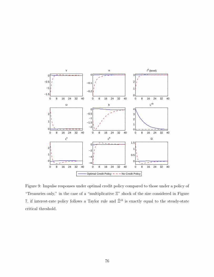
0 8 16 24 32 40

−1.5

−1

−0.5

0

Y

0 8 16 24 32 40

−0.2

−0.1

0

π

0 8 16 24 32 400

1

2

3

id (level)

0 8 16 24 32 400

1

2

ω

0 8 16 24 32 40

−2

−1.5

−1

−0.5

0

b

0 8 16 24 32 400

1

2

3

4

Lcb

0 8 16 24 32 40

0

1

2

cs

0 8 16 24 32 40

−6

−4

−2

0

cb

0 8 16 24 32 40

0

0.5

1

1.5

Ω

Optimal Credit Policy No Credit Policy

Figure 9: Impulse responses under optimal credit policy compared to those under a policy of

“Treasuries only,” in the case of a “multiplicative Ξ” shock of the size considered in Figure

7, if interest-rate policy follows a Taylor rule and Ξcb is exactly equal to the steady-state

critical threshold.

76

0 8 16 24 32 40

−0.4

−0.2

0

Y

0 8 16 24 32 40

0

0.02

0.04

0.06

π

0 8 16 24 32 400

1

2

3

id (level)

0 8 16 24 32 400

1

2

ω

0 8 16 24 32 40

−2

−1.5

−1

−0.5

0

b

0 8 16 24 32 400

1

2

3

4

Lcb

0 8 16 24 32 40

0

1

2

3

cs

0 8 16 24 32 40

−3

−2

−1

0

cb

0 8 16 24 32 40

0

0.5

1

1.5

Ω

Optimal Credit Policy No Credit Policy

Figure 10: Impulse responses under optimal credit policy compared to those under a policy of

“Treasuries only,” with the same disturbance as in Figure 9, but under optimal interest-rate

policy. Again Ξcb is exactly equal to the steady-state critical threshold.

77

0 8 16 24 32 40

−0.4

−0.2

0

Y

0 8 16 24 32 40

0

0.02

0.04

0.06

π

0 8 16 24 32 400

1

2

3

id (level)

0 8 16 24 32 400

1

2

ω

0 8 16 24 32 40

−2

−1.5

−1

−0.5

0

b

0 8 16 24 32 400

1

2

3

Lcb

0 8 16 24 32 40

0

1

2

3

cs

0 8 16 24 32 40

−3

−2

−1

0

cb

0 8 16 24 32 40

0

0.5

1

1.5

Ω

Optimal Credit Policy No Credit Policy

Figure 11: Impulse responses under optimal credit policy and under “Treasuries only,” for

the same disturbance and interest-rate policy as in Figure 10, but when Ξcb is 10bp higher

than the steady-state critical threshold.

78

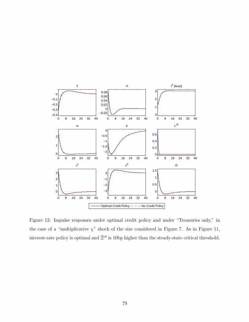
0 8 16 24 32 40−0.4

−0.3

−0.2

−0.1

0

Y

0 8 16 24 32 40

−0.020

0.020.040.060.08

π

0 8 16 24 32 400

1

2

3

id (level)

0 8 16 24 32 400

1

2

ω

0 8 16 24 32 40

−2

−1.5

−1

−0.5

0

b

0 8 16 24 32 400

0.2

0.4

0.6

Lcb

0 8 16 24 32 40

0

1

2

3

cs

0 8 16 24 32 40

−3

−2

−1

0

cb

0 8 16 24 32 40

0

0.5

1

1.5

Ω

Optimal Credit Policy No Credit Policy

Figure 12: Impulse responses under optimal credit policy and under “Treasuries only,” in

the case of a “multiplicative χ” shock of the size considered in Figure 7. As in Figure 11,

interest-rate policy is optimal and Ξcb is 10bp higher than the steady-state critical threshold.

79

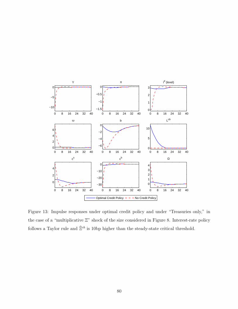
0 8 16 24 32 40

−10

−5

0

Y

0 8 16 24 32 40

−1.5

−1

−0.5

0

π

0 8 16 24 32 400

1

2

3

id (level)

0 8 16 24 32 400

2

4

6

ω

0 8 16 24 32 40

−6

−4

−2

0

b

0 8 16 24 32 400

5

10

Lcb

0 8 16 24 32 40

0

2

4

cs

0 8 16 24 32 40

−30

−20

−10

0

cb

0 8 16 24 32 40

0

1

2

3

4

Ω

Optimal Credit Policy No Credit Policy

Figure 13: Impulse responses under optimal credit policy and under “Treasuries only,” in

the case of a “multiplicative Ξ” shock of the size considered in Figure 8. Interest-rate policy

follows a Taylor rule and Ξcb is 10bp higher than the steady-state critical threshold.

80

0 8 16 24 32 40

−10

−5

0

Y

0 8 16 24 32 40

−1.5

−1

−0.5

0

π

0 8 16 24 32 400

1

2

3

id (level)

0 8 16 24 32 400

2

4

6

ω

0 8 16 24 32 40

−6

−4

−2

0

b

0 8 16 24 32 400

1

2

3

4

Lcb

0 8 16 24 32 40

0

2

4

6

cs

0 8 16 24 32 40

−30

−20

−10

0

cb

0 8 16 24 32 40

0

1

2

3

4

Ω

Optimal Credit Policy No Credit Policy

Figure 14: Impulse responses in the case of a “multiplicative χ” shock of the size considered

in Figure 8, under the same assumptions as in Figure 13.

81

0 8 16 24 32 40

−10

−5

0

Y

0 8 16 24 32 40

−1.5

−1

−0.5

0

π

0 8 16 24 32 400

1

2

3

id (level)

0 8 16 24 32 400

2

4

6

ω

0 8 16 24 32 40

−6

−4

−2

0

b

0 8 16 24 32 400

2

4

Lcb

0 8 16 24 32 40

0

2

4

6

cs

0 8 16 24 32 40

−30

−20

−10

0

cb

0 8 16 24 32 40

0

1

2

3

4

Ω

Optimal Credit Policy No Credit Policy

Figure 15: Impulse responses in the case of an “additive χ” shock of the size considered in

Figure 8, under the same assumptions as in Figure 13.

82