The Causal Effect of Education on Wages Revisited

1© Blackwell Publishing Ltd and the Department of Economics, University of Oxford 2012. Published by Blackwell Publishing Ltd,9600 Garsington Road, Oxford OX4 2DQ, UK and 350 Main Street, Malden, MA 02148, USA.

OXFORD BULLETIN OF ECONOMICS AND STATISTICS, 0305-9049doi: 10.1111/j.1468-0084.2012.00708.x

The Causal Effect of Education on Wages Revisited*

Matt Dickson

UCD Geary Institute, University College Dublin, Belfield, Dublin 4, Ireland(e-mail: [email protected])

Abstract

This study estimates the return to education in Britain using two instrumental variable (IV)estimators: one exploits variation in schooling associated with early smoking, the otheruses the raising of the school leaving age; both affect a sizeable proportion of the sample.Early smoking is found to be a strong and valid IV and unlike previous IV strategies usesvariations in education at numerous points across the distributions of (i) education, and(ii) ability. Thus whilst still a ‘local average treatment effect’ the estimate is closer to theaverage effect of additional education, akin to least squares but corrected for endogeneity.

I. Introduction

The causal effect of education on wages has long been a parameter of interest not onlyto labour economists but also to governments and individuals themselves. Much ink hasbeen spent and many regressions run in pursuit of an answer yet consensus remainselusive. Restricting focus to estimates of returns in the UK, the range varies from the verylow (Devereux and Hart, 2010) to the perhaps surprisingly high (Harmon and Walker,1995). Choice of econometric technique – and more specifically for instrumental variablesstudies, the choice of instrument – is non-trivial and has implications both for the size ofthe estimate and its external validity.

This study estimates the causal effect of education on wages using two alternative meth-ods of instrumentation. Estimates derived using variations in schooling associated withearly smoking behaviour are compared with estimates derived by exploiting the impact onschooling of the 1972 raising of the minimum school leaving age (RoSLA) in England andWales. The RoSLA instrument follows in the tradition of Card (1995) and similar studies,1

which use institutional factors or elements of the budget constraint to create instruments.This earlier research using IV methods covers a wide range and it is well established thatwhen the effect of treatment is heterogeneous, IV estimates a ‘local average treatment

ÅThanks to two anonymous referees for useful comments and also to seminar participants at University of War-wick, the Centre for Market and Public Organisation, the Work and Pensions Economics Group, EALE and IWAEE.Thanks also to the ESRC who provided the funding for this research under grant PTA-026-27-2132.

JEL Classification numbers: I20 J301The first notable study to use instrumental variables to estimate the return to education was Angrist and Krueger

(1991) while Harmon and Walker (1995) were the first to exploit changes in the minimum school leaving age in theUK to form IVs.

2 Bulletin

effect’ (LATE).2 The LATE will be instrument-dependent and captures the effect of thetreatment only for those induced to change treatment status by the particular instrumentchosen. These IV estimates of the return to education may only apply to quite a specificand unrepresentative group, for example, RoSLA affected only those who had wanted toleave school early therefore in this case IV estimates the effect of additional schooling forthose at the bottom of the schooling distribution who were forced to stay longer.

In contrast, early smoking is correlated with the schooling decisions of individualsacross the distributions of both (i) education and (ii) ability. We interpret the estimatesfrom this IV as closer to an average effect of additional schooling akin to least squares butcorrected for endogeneity. Our contribution is therefore two-fold: first, we present the casethat the early smoking IV LATE is more appropriate than the RoSLA LATE for drawinginference concerning the average return to education in the population, implementing eachIV using that same data from the British Household Panel Survey. Second, as we havetwo genuinely different mechanisms generating variation in education and providing twoinstruments, we are able to test the validity of the exclusion restrictions, something that israrely possible to do. We find the ordinary least square (OLS) estimate to be considerablydownward biased at 4.6% compared with the IV estimates of 12.9% using early smoking,10.2% using RoSLA and 12.5% using both instruments simultaneously. This suggests thatschooling in Britain has a high wage return not only at the lower part of the distributionbut across a range of education levels.

The next section considers the problem of estimating the return to education and IVsolutions in the literature. Section III establishes the case for early smoking as an instru-ment for education. Section IV describes the data and estimation approach, while section Vpresents the results before evaluating various hypotheses regarding the instrument. SectionVI then compares the early smoking instrument estimates with RoSLA IV results, beforesection VII exploits the presence of two instruments to formally test the validity of theseinstruments. Section VIII offers some concluding remarks.

II. Literature

The foundation of the education returns literature has been Mincer’s (1974) human capitalearnings function:

lnwi =X ′i �+�Si + εi (1)

in which wi is the wage, Xi is a vector of the individual’s characteristics, including expe-rience and experience-squared and Si is the number of years of schooling, determinedby:

Si =X ′i �+ui (2)

It is well known that if this relationship in equation (1) is estimated by least squares, acausal interpretation of the estimated parameter � requires E(Xiεi)=0 and E(Siεi)=0, thelatter of which entails E(uiεi)=0.

2See Imbens and Angrist (1994) for the theoretical exposition of LATE.

© Blackwell Publishing Ltd and the Department of Economics, University of Oxford 2011

The causal effect of education 3

The potential for the unobserved characteristics that determine schooling choice to alsobe correlated with wage is an obvious concern. Early research concentrated on the issueof ‘ability bias’ which suggested that E(uiεi) > 0 since the residuals pick up ability whichis positively correlated with both wages and schooling, resulting in OLS estimates beingunambiguously biased upwards. In contrast, Griliches (1977) concluded that ‘ability bias’was in reality small and was overwhelmed by the attenuation bias introduced by measure-ment error in the schooling variable, with the result that OLS under-estimated the actualreturn to education.

At the start of the 1990s, a number of economists suggested that OLS estimates ofthe return to education may suffer from a further bias – ‘discount rate bias’ (see Lang,1993; Card, 1994). In Becker’s (1964) model of human capital formation, with standardassumptions,3 an individual will accumulate human capital to the point where the marginalrate of return on the last unit of education is equal to his/her discount rate. An individual’sdiscount rate reflects both his/her access to finance to fund current investment in educa-tion whilst deferring earnings and also his/her rate of time preference. If individuals differin their preferences and in their financial resources, this will result in different discountrates and lead to variation in the point at which they stop acquiring education – a higherdiscount rate resulting in a lower optimal level of education. Therefore schooling choicemay differ amongst individuals of the same ability because of differences in individualdiscount rates. If the unobserved discount rate that affects education also independentlyaffects wages then OLS estimates will incur bias from this source.

It could be the case that individuals who have a higher discount rate have more ambitionor determination to get into the labour market and earn money. This drive is rewarded inhigher wages and also these individuals are more likely to choose career paths with steepwage curves. Consequently a higher discount rate is associated with lower education butalso a higher wage conditional on education, thus E(uiεi) < 0 and OLS estimates of thereturn to education will be negatively biased.

Discount rate and ability are both sources of variation in levels of schooling, moreoverthey interact. Though (arguably) unconditionally uncorrelated, Lang (1993) points out thatonce we condition on a level of education, discount rate and ability are correlated: thosewith a higher discount rate will have higher ability. Recalling Becker’s model this makessense: if two individuals have chosen the same level of schooling it means that for each,at that point, the marginal return to schooling is equal to their discount rate. Thus theindividual with the higher discount rate has a higher marginal return at that level of edu-cation, indicating that they have higher ability. A higher value of discount rate will reduceschooling, but conditional on schooling in the wage equation, a higher discount rate willmean higher ability and a higher wage: thus E(uiεi) < 0. This potential mechanism throughwhich discount rate affects the joint process of education and earnings again suggests anegative bias in the OLS estimates. If both ability bias and discount rate bias affect theOLS estimate of the return to education but work in opposite directions, then a priori thenet bias in the coefficient is indeterminate.

3(i) workers maximize the discounted present value of lifetime wealth; (ii) time in school is independent of timein work, or alternatively lifetimes are infinitely lived; (iii) there are no direct costs of education; (iv) the effect ofexperience on earnings is multiplicative.


4 Bulletin

Much of the literature has focused on the IV solution to this endogeneity problem:identifying a variable which affects schooling but does not independently enter into theearnings equation, and is uncorrelated with its error term. However, while IV has theadvantage that we can potentially derive estimates purged of the biases discussed above,it also has some shortcomings. Weak instruments (i.e. those that although uncorrelat-ed with wages are hardly correlated with schooling) and invalid instruments (those thatalthough correlated with schooling, may also be correlated with wages) may be worsethan no instruments at all – as Bound et al. (1993) put it ‘the cure can be worse than thedisease’.

Much attention has been given to the weak instruments issue in the econometrics lit-erature of the last 15 years and it is now well known (see inter alia Murray, (2006),Baum et al. (2007)) that two-stage least squares performs very poorly in the presenceof weak instruments: not only are point estimates biased, the estimated standard errors ofparameters are too small, leading to inaccurate inference. Furthermore, Bound et al. (1995)show that even a small correlation between the instrument and the error term in the earningsequation can result in a large bias in the IV estimates even in large samples – a problemthat is compounded if the instrument is weak.

It is not routinely possible however to test an instrument for correlation with the errorterm in the earnings equation as to do that we would first need to estimate the wage equa-tion to give us a valid error term which requires a consistent estimator for � and �, whichwe can only find if we have an alternative instrument that we know is valid and strongin the first place. The advantage in having multiple instruments is that this allows us todetermine the validity of the preferred instrument (early smoking), exploiting the validityof the other instrument available (RoSLA). In addition to the formal econometric test,further supportive evidence for the validity of the early smoking instrument is provided bythe reduced forms, by intuition and by the consistency of results estimated with differentinstruments.

As outlined above, an additional problem with IV in the presence of heterogeneoustreatment response is that it captures a LATE: the IV estimate of the schooling coefficient� is a weighted average of the marginal returns to education for those whose schoolingchoice is influenced by the instrument, conditional on Xi.4 It is well established, for exam-ple, that estimates derived using the 1972 RoSLA capture the return to one additional yearof education for those at the lower end of the schooling distribution: there was no rippleeffect further up (see inter alia Harmon and Walker, (1995) Grenet, (2012)). Thus whilecontributing useful information regarding the return for specific groups, previous LATEestimates have provided little indication of what the return to schooling may be for a moregeneral population.

Therefore it is important that any candidate instrument avoids these three prominentproblems: being correlated with the structural equation error term, being only weaklycorrelated with the endogenous regressor or capturing a LATE that is not informativewhen it comes to answering the question we want to ask.

4In order to give this LATE interpretation, there is a monotonicity requirement that all individuals have the samesigned response to the instrument.



III. Instrumenting education using early smoking

Evans and Montgomery (1994) proposed using whether or not an individual smoked whenthey were young as an instrument for schooling.5 The intuition behind the instrumentstarts with the observation that just as schooling is not randomly assigned across the popu-lation, neither is the decision to engage in (un)healthy habits. Evans and Montgomery notethat ‘one of the most persistent relationships in health economics is that more educatedpeople have better health and better health habits’ (1994, p.1). This view is supported by anumber of reviews of the empirical evidence on the link between health and education byGrossman (2006).After extensively reviewing the evidence Grossman concludes that com-pleted years of formal schooling is the most important correlate of good health, and thisstatement applies whether health is being measured by mortality rates, morbidity rates,self-evaluated health status or psychological well being. In the UK, Oreopoulos (2006)uses data from the general household survey (GHS) which asks individuals to self-reporttheir health status, and finds that an additional year of schooling increases the chance thatan individual will report good health by 6.0 percentage points, and reduces the chanceof reporting poor health by 3.2 percentage points. There remains a debate as to whetheror not this education–health relationship is causal, with Evans and Montgomery citinga quite different explanation, proposed by Fuchs (1982). Fuchs argues that unobserveddifferences in the rate of time preference determine both the number of years schoolingthat an individual attains and their investments in health, as both decisions involve a tradeoff between current costs and the discounted value of future benefits.

As with Becker’s model of human capital accumulation, in a health accumulation modelindividuals invest in health until the marginal return to health investment equals their dis-count rate. If an individual has a higher discount rate because of her rate of time preference,she cares less about the future and more about the present and will therefore ceteris paribusquit formal education at a younger age and be less (more) likely to engage in good (bad)health habits. If the correlation between a health habit, such as smoking, and educationis driven by a common unobserved factor (time-preference) then this health habit couldpotentially be used as an instrument for education.

In their work on rational addiction Becker and Murphy (1988) posit that the decisionto smoke reflects discount rate in that it indicates an individual’s rate of time preference;we follow Evans and Montgomery in arguing that, as a result, smoking as a teenagercan be used as a valid instrument for education. One way in which Fuchs supported hishypothesis was to show that education at age 24, when education levels vary considerably,is as important a predictor of smoking at 17 – when most individuals have the same levelof education – as it is a predictor of smoking at 24 (see Farrell and Fuchs, 1982). Usinga larger dataset than the main estimation sample, we implement a probit of current smok-ing using completed years of schooling amongst the explanatory variables, and repeat theprobit for smoking at age 16. The marginal effects estimated at the mean of the explana-tory variables suggest that for each additional year of schooling the probability of being acurrent smoker falls by 2.7% (significant at the 1% level). In the probit for smoking at 16,it is estimated that each additional year of completed education reduces the probability of

5This IV strategy has also been pursued by Chevalier and Walker (2002) using GHS and National Child Develop-ment Study (NCDS) data, and by Fersterer and Winter-Ebmer (2003) for Austrian data.


6 Bulletin

having smoked at age 16 by 3.8% (significant at the 1% level).6 Thus completed educationis a significant determinant of early smoking – suggesting that it is not greater educationthat determines the decision not to smoke: education predicts early smoking as well aslater smoking, suggesting that another underlying factor (time preference) is determiningboth.

Intuitively, the decision that an individual makes at age 16 as to whether or not tocontinue in education is likely to be significantly affected by her discount rate – whetherthat is because of access to financial resources or because of the individual’s rate of timepreference. In the UK this is the first point at which individuals can choose to leave edu-cation, moreover it remains the case that staying in school post-16 and taking A-levelsis the major route into university. Moreover, whether an individual chooses to smoke at16 is also likely to be determined in large part by their rate of time preference. Of thesample individuals who have ever smoked, 60.5% were smoking when age 16 and 81.1%were smoking when age 18.7 Therefore it is clear that the majority of individuals who eversmoke first take that decision at around the same time that they are making decisions overthe continuation of their education. This concurrence in the timing of the smoking andschool leaving decisions generates a statistically precise and quantitatively large correla-tion between years of education and early smoking. Thus smoking at 16 satisfies the firstcriterion for an instrument: it is relevant. Moreover, the effect of early smoking on yearsof schooling is sizeable, just under 1 year less education is completed on average by thosewho smoke when 16 ceteris paribus, therefore the instrument works through a substantialvariation in education.

In addition to looking at the first stage equation for years of schooling, looking atthe reduced form for the dependent variable of interest (log hourly wage), supports theargument that early smoking can be used to instrument for education. The smoker-at-16indicator has a significant (at 1% level) negative coefficient (−0.113) in the reduced formregression,8 which is in line with intuition: those who smoked when 16 have lower wagesthan those who did not, with the argument being that this is driven wholly by the differencein average years of schooling between the two groups.

The second criterion is validity: the instrument must not be correlated with wage. As itis a past health habit that is instrumenting for education in the equation for current wage,there should not be a correlation via an income effect: the contemporary wage can have noimpact on the disposable income of 16-year old deciding whether or not to smoke. More-over, theoretically whether one smoked at 16 should have no independent direct effect oncurrent wage. It is by no means certain that current smoking affects current wage via aproductivity effect – in fact, using British Household Panel Survey (BHPS) data Brune(2007) shows that there is only weak evidence that current smoking causally reducescurrent wages. Thus a link between smoking at 16 and current wage would be evenmore speculative.

Further support for this contention comes from evidence in the literature that there areno harmful effects of early drug and alcohol use on later economic prospects. Burgess and

6Full tables of results available in Dickson (2009).7These figures refer to the estimation sample, for the largest sample available in the BHPS the figures are almost

identical: 61.0% and 79.7%.8All robustness check results are available in Dickson (2009).



Propper (1998) show this for adolescent men in the US whose economic outcomes 10 yearslater are unaffected by soft drug and alcohol use, while MacDonald and Pudney (2000)show similar results for young British men. Taking all of this into consideration, there isno reason to think that smoking at 16 would affect current wage – and as individuals ageand move further away from being 16 this is even more so the case. Moreover, there is agood degree of movement between smoking and non-smoking amongst the BHPS sampleof men, with 41.0% of men who did smoke when they were 16 having stopped by thetime they are first observed in the data, while 37.5% of the men who are smokers whenfirst observed in the data were not smokers at age 16. In fact, of the 585 men who changesmoking status between 16 and their first panel observation, 46.3% are taking up smok-ing. In light of these arguments, we believe that smoking at 16 can itself be legitimatelyexcluded from the wage equation.

The next important question is whether early smoking is correlated with otherunobservable characteristics that do affect current wage. If the rate of time preferencethat characterizes early smokers leads to other unobserved human capital investmentsthroughout life that independently affect wage then this would invalidate the instrument.Alternatively it may be the case that time-preference at age 16 affects investment in edu-cation but that conditional on this there is not an additional effect on earnings. Evidencefrom the psychology and psychiatry literatures suggests that for men in particular, timehorizons during the teenage years are often shorter than is the case later in life and thattime-preferences do not settle until men are in their early 20s (see Silverman, (2003); Readand Read, (2004) Steinberg, (2007)). This would lower the correlation between teenageand adult time-preferences for an individual, thus if there is an independent (of education)effect of time-preference on wages, this may not be correlated with education decisionsmade when 16. Furthermore, recent work by Grafova and Stafford (2009), examining thewage effects of smoking history in the US, suggest that conditional on education there isno difference in wages between those who never smoke and those who smoke earlier inlife but then give up. Anger and Kvasnicka (2010) for Germany and Brune (2007) for theUK find analogous results. This also suggests that – at least for those who later quit – earlysmoking does not indicate unobservable characteristics and investments that will influ-ence later wages. The substantial degree of movement between smoking status at 16 andsmoking status when an individual is observed in the data also implies that the correlationbetween early smoking and later unobserved characteristics is not clear cut.

Finally, given that we have more than one instrument the system is over identifiedand we can exploit this to econometrically test for a correlation between early smokingand the unobservables in the wage equation. Section VII details the results of numerousapproaches to investigating such a correlation, each of which support the conclusion thatearly smoking is a valid instrument for education.9

9Bonjour et al. (2003) use data from St Thomas’ Hospital’s Adult Twins Registry to estimate returns to education,and also exploit information on early smoking behaviour to consider whether this can be used as a valid instrument.Bonjour et al. conclude that early smoking is picking up family background rather than time-preference, howevertheir sample is comprised almost exclusively of female twins. Though it may be the case that for young females –where historically smoking prevalence has been lower – early smoking is more of a reflection of background thantime-preference, this is less likely to be the case for young men, moreover the background/ability arguments aretackled below.


8 Bulletin

If we accept that early smoking satisfies these two criteria of relevance (and non-weakness) and validity then an indicator for early smoking can be used as an instrument:influencing schooling through changing the marginal costs of schooling in a way which isconditionally uncorrelated with the unobservables.

Furthermore, though it captures a LATE – the return for a group of individuals whohave lower education because of a higher than average discount rate – it is shown belowthat this is a group comprised of individuals across the education distribution and of allabilities, thus the estimate is arguably more representative of the return for the populationas a whole than estimates identified by alternative IV estimation strategies.

IV. Data and estimation

The data come from the BHPS which is a nationally representative survey of the pop-ulation which began in 1991 and follows the sample individuals each year. In 1999, inaddition to the core survey there was a supplementary component in which questions wereasked regarding previous health habits. This allows the creation of a 15-wave pooled-paneldataset containing variables describing individuals’ characteristics, a dummy to indicatewhether the individual smoked when 16, education, and current hourly wage rate. Sincethe previous health habits question was only asked in wave 9, the constructed panel onlycontains observations from individuals present in that wave, but for these individuals allof their available observations are included. The sample includes males who are in full-time employment (30+ hours/week), are not self-employed and are in the age range 19–65inclusive.10

There are issues of measurement error when using number of years of schooling as themeasure of education, however in order to make the results comparable with the major-ity of the literature the number of years of schooling is used as the education variable.11

With respect to earnings, it is standard to use the log of hourly earnings and so again forcomparability this is what is used – the log of real wage (using, 2006 pounds as the base).12

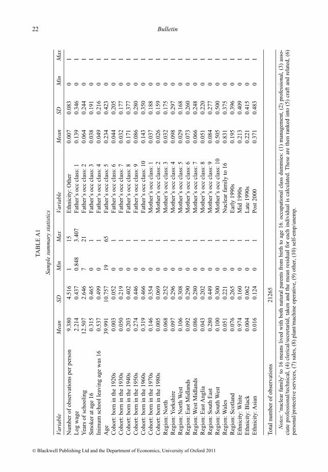
The pooled-panel dataset constructed contains 21,256 observations from 2,266 maleswith each individual having between 1 and 15 observations; the mean number of obser-vations per individual is 9.38, median 10. In all of the regressions standard errors areclustered at the level of the individual.13 Appendix Table A1 contains summary statisticsfor the estimation sample.

10This age range captures ‘prime-age’ males and ensures that smoking at 18 is not the same as current smokingfor any individuals, as smoking at 18 will be used as an instrument in a robustness check.

11Formally: Years-of-schooling = (age left education − 5); thus we assume a school start age of 5, which is thecompulsory school start age in the UK. For more details of the variables construction see Appendix A.

12The log wage distribution is trimmed such that the top and bottom 1% within each year are excluded.13In order to avoid issues around differential attrition, we have re-estimated the models using both inverse prob-

ability weighting and also including in the regressions a variable indicating the number of observations that eachindividual has, and in each case the results remain. As the first stage involves regression of years-of-schooling –which is time-invariant – on characteristics, we re-estimate the model using just one observation (their first) for eachmember of the sample but then all of the observations in the second stage, bootstrapping to get the correct standarderrors in each stage. There is no substantive change in the conclusions. Similarly the models can be estimated onany single wave and the nature of the results does not change. All of these robustness check results are available inDickson (2009).



We begin by estimating the conventional human capital earnings function where thedependent variable is the natural log of real hourly wage, and the explanatory variablesare age, age-squared and years-of-schooling.14 Also included are controls for ethnicity, forregion (using the 10 standard regions) in order to pick up regional real wage differentials,year-of-birth15 and its square to pick up cohort effects and dummies for parental charac-teristics. The parental characteristics included are the standard occupational classificationof the job of both the individual’s father and mother when the individual is 14 years ofage, and a dummy to indicate that the individual lived with both natural parents from birthup to the age of 16. These parental characteristics are included since in their absence thesmoking at 16 variable could be picking up background characteristics correlated witheducation and smoking at 16. Including year dummies in the model would be problematicsince both age and year-of-birth are included, however controls are included for whetherit was the early-, mid-, late-1990s or post-2000 to allow for business cycle effects.16

V. Results and analysis

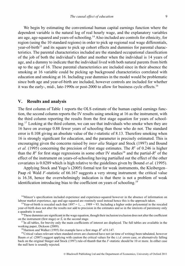
The first column of Table 1 reports the OLS estimate of the human capital earnings func-tion, the second column reports the IV results using smoking at 16 as the instrument, withthe third column reporting the results from the first stage equation for years of school-ing.17 Looking at the third column, we can see that individuals who smoke when they are16 have on average 0.88 fewer years of schooling than those who do not. The standarderror is 0.108 giving an absolute value of the t-statistic of 8.13. Therefore smoking when16 is strongly significant for education, and the parameter is precisely estimated. This isencouraging given the concerns raised by inter alia Staiger and Stock (1997) and Boundet al. (1995) concerning the precision of first stage estimates. The R2 of 0.246 is higherthan the R2 for first stage regressions in some other IV studies18 and the partial-R2 of theeffect of the instrument on years-of-schooling having partialled out the effect of the othercovariates is 0.0289 which is high relative to the guidelines given by Bound et al. (1995).

Applying Stock and Yogo’s (2005) formal test for weak instruments, the Kleibergen–Paap rk Wald F-statistic of 66.167 suggests a very strong instrument: the critical valueis 16.38, hence the overwhelmingly indication is that there is not a problem of weakidentification introducing bias to the coefficient on years of schooling.19

14Mincer’s specification included experience and experience-squared however in the absence of information onlabour market experience, age and age-squared are routinely used instead hence this is the approach taken.

15Year-of-birth is rescaled such that 1897 = 1,. . ., 1989 = 93. Including a higher order polynomial in the rescaledyear-of-birth does not alter the results nor add to precision in the estimates and so in the interests of parsimony onlya quadratic is used.

16These dummies are significant in the wage equation, though their inclusion/exclusion does not alter the coefficienton the instrument (first stage) or Si in the second stage.

17In all tables, for brevity only the main coefficients of interest are displayed. The full tables are available in theworking paper, Dickson (2009).

18Harmon and Walker (1995) for example have a first stage R2 of 0.147.19Critical values relevant when standard errors are clustered have not (at time of writing) been tabulated, however

Baum et al. (2007) suggest applying with caution the critical values for the i.i.d. errors case, or alternatively fallingback on the original Staiger and Stock (1997) rule-of-thumb that the F-statistic should be 10 or more. In either casethe null here is soundly rejected.


10 Bulletin

TABLE 1

OLS and IV returns to education estimates for log hourly wage: fullset of controls BHPS, Males, age 19–65

Smoker at 16 RoSLA Both

OLS IV (first stage) IV (first stage) IV (first stage)

Years of schooling 0.046*** 0.129*** — — 0.102** — — 0.125*** — —(0.003) (0.020) (0.051) (0.019)

Smoker at 16 indicator — — — — −0.876*** — — — — — — −0.874***

(0.108) (0.107)min. school LA=16 — — — — — — — — 0.564*** — — 0.556***

(0.206) (0.202)R2 0.265 0.072 0.246 0.177 0.227 0.088 0.250F-test on exclusion — — — — 66.17 — — 7.49 — — 36.83of instrument(s)Partial R2 of the — — — — 0.0289 — — 0.0044 — — 0.0332instrument(s)

Hansen J -test of overidentification 0.202, P-value = 0.6529

Notes: All regressions: 21,256 observations from 2,266 individuals. Robust standard errors clustered at individuallevel in parenthesis. *** Significant at the 1% level,** significant at the 5% level,*significant at the 10% level. Controlsincluded: age, age2, year-of-birth, year-of-birth2, region dummies (10 regions), ethnicity dummies (White, Black,Asian, other), survey period dummies (early 1990s, mid 1990s, late 1990s, post 2000), dummy for lived with bothnatural parents from birth to age 16,each parents’ occupational class dummies: (1) management, (2) professional,(3) associate professional/technical, (4) clerical/secretarial, (5) craft and related, (6) personal/protective services, (7)sales, (8) plant/machine operative, (9) other, (10) self-emp/unemp. All regressions include a constant.

Turning to columns 1 and 2, the OLS estimate suggests that an additional year of school-ing increases wage by 4.6% whereas the IV estimate of the return is 12.9%. We expectthat the IV results will be less precisely estimated than the OLS, and while the standarderror on years of schooling in the instrumented regression does increase, the coefficientremains precisely estimated and significant at all conventional levels. Estimation of theIV using the Fuller-LIML estimator rather than standard 2SLS-IV, in order to be as robustas possible to any potential bias in the IV estimates, does not result in any substantivechange to the estimated coefficients or standard errors: the return to schooling in the IVestimation remains 12.9, standard error of 0.020.20 The estimates of a 4.6% return by OLSrising to 12.9% by IV are in line with those found in majority of other studies using UKdata, particularly Harmon and Walker (1995, 1999).

More recently Devereux and Hart (2010) have used both the GHS and the New Earn-ings Survey Panel Dataset to re-assess returns to education estimates using the 1947 raisingof the school leaving age in England from 14 to 15. They implement a Two Sample TwoStage Least Squares approach and find very low returns for men, in the order of 3–4%.Devereux and Hart suggest that the low return may be due to the leaving age of 15 notcoinciding with any exit exams; moreover, this reform affected a cohort of individuals ageneration older than those in our data. Grenet (2012) exploits the 1972 RoSLA and usingLabour Force Survey data finds a return for men in the range of 7–8%. The 1972 RoSLAIV estimate we find in the BHPS is 10.2%, which is slightly above Grenet’s estimate, withthe early smoking estimate higher still, however this is in line with the early smoking IV

20The modified LIML estimator introduced by Fuller (1977), with the Fuller parameter, a, set to 1 is regarded asmost robust to any potential weakness of the instrument. Results available in Dickson (2009).



OLS IV Instrument

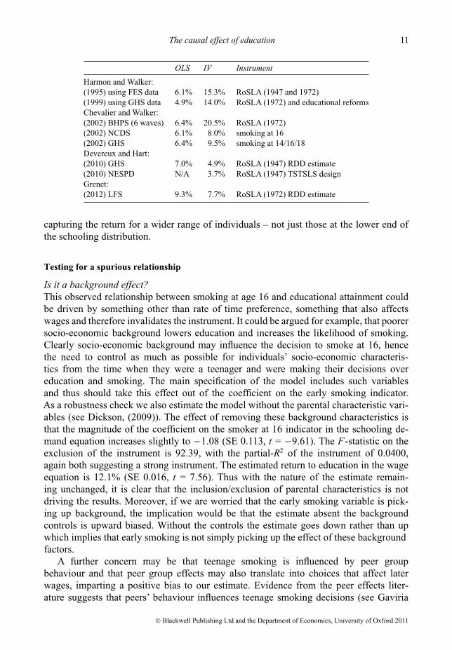
Harmon and Walker:(1995) using FES data 6.1% 15.3% RoSLA (1947 and 1972)(1999) using GHS data 4.9% 14.0% RoSLA (1972) and educational reformsChevalier and Walker:(2002) BHPS (6 waves) 6.4% 20.5% RoSLA (1972)(2002) NCDS 6.1% 8.0% smoking at 16(2002) GHS 6.4% 9.5% smoking at 14/16/18Devereux and Hart:(2010) GHS 7.0% 4.9% RoSLA (1947) RDD estimate(2010) NESPD N/A 3.7% RoSLA (1947) TSTSLS designGrenet:(2012) LFS 9.3% 7.7% RoSLA (1972) RDD estimate

capturing the return for a wider range of individuals – not just those at the lower end ofthe schooling distribution.

Testing for a spurious relationship

Is it a background effect?This observed relationship between smoking at age 16 and educational attainment couldbe driven by something other than rate of time preference, something that also affectswages and therefore invalidates the instrument. It could be argued for example, that poorersocio-economic background lowers education and increases the likelihood of smoking.Clearly socio-economic background may influence the decision to smoke at 16, hencethe need to control as much as possible for individuals’ socio-economic characteris-tics from the time when they were a teenager and were making their decisions overeducation and smoking. The main specification of the model includes such variablesand thus should take this effect out of the coefficient on the early smoking indicator.As a robustness check we also estimate the model without the parental characteristic vari-ables (see Dickson, (2009)). The effect of removing these background characteristics isthat the magnitude of the coefficient on the smoker at 16 indicator in the schooling de-mand equation increases slightly to −1.08 (SE 0.113, t = −9.61). The F-statistic on theexclusion of the instrument is 92.39, with the partial-R2 of the instrument of 0.0400,again both suggesting a strong instrument. The estimated return to education in the wageequation is 12.1% (SE 0.016, t = 7.56). Thus with the nature of the estimate remain-ing unchanged, it is clear that the inclusion/exclusion of parental characteristics is notdriving the results. Moreover, if we are worried that the early smoking variable is pick-ing up background, the implication would be that the estimate absent the backgroundcontrols is upward biased. Without the controls the estimate goes down rather than upwhich implies that early smoking is not simply picking up the effect of these backgroundfactors.

A further concern may be that teenage smoking is influenced by peer groupbehaviour and that peer group effects may also translate into choices that affect laterwages, imparting a positive bias to our estimate. Evidence from the peer effects liter-ature suggests that peers’ behaviour influences teenage smoking decisions (see Gaviria


12 Bulletin

and Raphael, 2001; Nakajima, 2007), however research using UK data also providessupport to an alternative view: that individuals choose to smoke and then choose like-minded peers (see De Vries et al., 2003). Ideally information on teenage peer groupwould be available in order to consider this channel of influence – though even then theendogeneity of peer group formation and smoking initiation would remain a problem – butunfortunately such variables are not available in our data. However, to the extent thatchildren from similar family backgrounds form peer groups, some peer effects will becontrolled for by the inclusion of parental background characteristics. Again, the fact thatthe point estimate of the return to education increases when parental characteristics areincluded indicates that absent these controls the estimate was not upward biased, which isreassuring.

Is it an ability effect?The correlation between smoking and education is also consistent with an alternativehypothesis: that those with lower unobserved ability will acquire less education and aremore likely to smoke. If it is the case that we are primarily picking up some measure ofability then we would expect that – by definition – smoking at 16 only affects the educationof individuals at the lower end of the ability distribution. However, if we assume that theresidual from the OLS log wage regression is a reasonable proxy for ability, we can dividethis residual distribution into quintiles and examine whether smoking at 16 is a featureonly of low ability (low residual) individuals or if it is something that individuals of allabilities engage in.

Table 2 shows the numbers who smoke at age 16 in each quintile of this residual logwage distribution. The left-side panel of the table shows that in the lowest quintile approx-imately 44% of the males smoked at 16. This figure falls to approximately 39% in the nextquintile up and the next after that (30%) before rising again in the fourth quintile (34%).Despite a fall in the last quintile, the figure for the percentage of individuals who smoked

TABLE 2

Smokers at 16/18 by quintile of the mean log wage residual distribution

Non-smoker Smoker Non-smoker SmokerQuintile at 16 at 16 Total at 18 at 18 Total

1 256 198 454 209 245 45456.39% 43.61% 100.00% 46.04% 53.96% 100.00%

2 278 175 453 216 237 45361.37% 38.63% 100.00% 47.68% 52.32% 100.00%

3 319 134 453 265 188 45370.42% 29.58% 100.00% 58.50% 41.50% 100.00%

4 299 154 453 255 198 45366.00% 34.00% 100.00% 56.29% 43.71% 100.00%

5 349 104 453 295 158 45377.04% 22.96% 100.00% 65.12% 34.88% 100.00%

Total 1501 765 2266 1240 1026 226666.24% 33.76% 100.00% 54.72% 45.28% 100.00%

Notes: OLS log wage regression (Table 1 column 1) run on pooled panel dataset, residualsare taken and the mean residual for each individual is calculated. These are then ranked intofive quintiles as a measure of unobserved ability.



at age 16 is still as high as 23% in the highest quintile of the residual log wage distribution.There are fewer smokers at 16 in the higher quintiles of the distribution, nevertheless thereremain substantial numbers of smokers at 16 in the highest quintiles which indicate thehighest ability individuals.

Continuing to use the log wage residual distribution as a proxy for ability, we can lookat the first stage schooling equations in each quintile. The left side of Table 3 shows that theeffect of smoking at 16 is actually increasing as we move up the distribution. In the lowestquintile, schooling is reduced by 0.77 years, this is equivalent to a reduction of 6.21% ofthe mean number of years of education in this group. In the second and third quintiles thereduction in education associated with early smoking is even greater both in absolute termsand relative to mean education in these quintiles. The fourth quintile is affected the leastby early smoking but still it is associated with three-quarters of a year less education, andin the highest quintile the estimated reduction is 0.88 years, 6.9% of mean education inthis quintile. Table 2 shows that there are significant numbers of individuals who smoke at16 in all of the quintiles thus these results are not due to small numbers of early smokers,and the coefficient on smoking at 16 is significant at the 1% level in all quintiles. Far from

TABLE 3

First stage IV regression coefficients on smoker at 16 indicator andminimum school leaving age of 16 indicator, by quintile of the mean log

wage residual distribution

IV (first stage): Smoking IV (first stage): RoSLA

Quintile Smoker at 16 R2 MSLA = 16 R2

1 −0.773*** 0.268 1.044** 0.262No.obs = 3,684 (0.265) (0.510)Mean years of schooling12.41

2 −1.044*** 0.317 0.837* 0.292No.obs = 4,285 (0.227) (0.458)Mean years of schooling12.09

3 −0.950*** 0.329 0.315 0.309No.obs = 4,461 (0.249) (0.496)Mean years of schooling12.30

4 −0.747*** 0.257 0.398 0.240No.obs = 4,496 (0.213) (0.388)Mean years of schooling12.28

5 −0.879*** 0.341 0.080 0.321No. obs = 4,330 (0.241) (0.435)Mean years of schooling12.65

Notes: ***signficant at 1% level,**significant at 5% level,*significant at 10% level.Robust standard errors clustered at individual level in parenthesis. Other covariatesincluded in regressions are as Table 1.


14 Bulletin

0.1

.2.3

.4

k de

nsity

10 11 12 13 14 15 16 17 18 19 20 21 22 23 24 25 26

Education leaving age

Smokers at 16 Non−smokers at 16

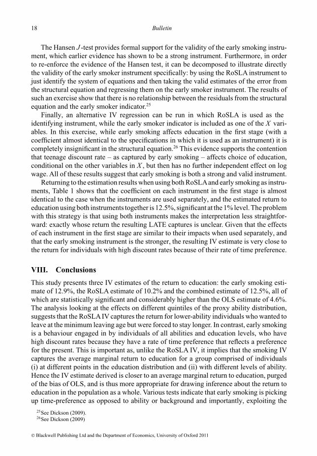
Figure 1: Education leaving age density, by smoker at 16 status

only affecting the low ability individuals, this evidence indicates that smoking at 16 has agreater absolute and relative effect on the highest ability individuals.

In addition, Figure 1 plots the density of education leaving age for smokers at 16 andnon-smokers at 16. If it was only low educated, low ability individuals who smoke at16 then we would expect the densities to look very different with very little mass in theupper ranges for the early smokers. However, while the density for non-smokers at 16does have a greater mass around 21 and less around 15/16 (suggesting more non-smokersgo to university), it is quite close to being a general right-ward shift of the distributioncompared with the smokers at 16.21 This all fits with the discount rate hypothesis whichsays that there are smokers and non-smokers at 16 of all abilities and that smoking at 16has an effect to reduce education at all points of the distribution.

To further pursue the hypothesis that individuals who have lower ability are likely toget less education and are more likely to smoke, the results are replicated using smokingat age 18 rather than smoking at age 16. Age 18 is the point at which individuals in the UKhave to decide whether to remain in education and go to university, and this decision islikely to be affected by their rate of time preference. Moreover, it is more difficult to arguethat smokers at 18 are more likely to be lower ability than higher ability individuals. Theright panel of Table 2 shows the numbers who smoke at age 18 in the quintiles of the logwage residual distribution. The table illustrates that in the lowest quintile the smokers at18 out number non-smokers (54% vs. 46%), and this remains the case in the next quintileup (52% smokers vs. 48% non). As with smoking at 16, the numbers who did smoke aregenerally lower as we move up the quintiles yet in the highest quintile, still as much as 35%of the individuals smoked at 18. In each quintile there are substantially more smokers at 18than there were at 16 – at least a 10 percentage point swing to smokers from non-smokers– supporting the idea that teenage smoking is a habit that high discount rate individuals ofall abilities engage in.

21It is true that younger cohorts have been acquiring more education and smoking less which would also lead to ashift of the curve to the right for non-smokers at 16, however repeating Figure 1 by cohort reveals the same patternin all cohorts, see Dickson (2009).



TABLE 4

OLS and IV returns to education estimates for log hourly wage: full set of controls BHPS, Males,age 19–65

Smoker at 18 Smoker at 17

OLS IV (first stage) IV (first stage)

Years of schooling 0.046*** 0.135*** — — 0.130*** — —(0.003) (0.023) (0.021)

Smoker at 18 indicator — — — — −0.745*** — — — —(0.108)

Smoker at 17 indicator — — — — — — — — −0.816***

(0.108)R2 0.265 0.042 0.242 0.067 0.245F-test on exclusion of instrument — — — — 48.02 — — 57.14Partial R2 of the instrument — — — — 0.0236 — — 0.0267

Notes: All regressions: 21,256 observations from 2,266 individuals. Robust standard errors clustered atindividual level in parenthesis.*** significant at the 1% level,** significant at the 5% level,*significant at the10% level. Controls included: age, age2, year-of-birth, year-of-birth2, region dummies (10 regions), ethnicitydummies (White, Black, Asian, other), survey period dummies (early 1990s, mid 1990s, late 1990s, post2000), dummy for lived with both natural parents from birth to age 16, each parents’ occupational classdummies: (1) management, (2) professional, (3) associate professional/technical, (4) clerical/secretarial,(5) craft and related, (6) personal/protective services, (7) sales, (8) plant/machine operative, (9) other, (10)self-emp/unemp. All regressions include a constant.

Results using smoking at 18 as the instrument are displayed in Table 4. Looking at thethird column, the first stage equation for schooling, smoking at 18 reduces education by0.75-years. This is lower than the corresponding reduction associated with smoking at 16but this is consistent with the time preference story: smokers at 18 have a higher discountrate than non-smokers at 18 but, ceteris paribus, smokers at 16 will have a higher discountrate than smokers at 18. If smokers at 18 have a lower discount rate relative to those whosmoke at 16, they will remain in education longer thus we expect that the reduction ineducation for smokers at 18 is not as much as it is for smokers at 16. The robust standarderror on smoking at 18 is 0.108, giving a t-statistic with an absolute value of 6.93, thereforethe parameter remains precisely estimated. The R2 for this first stage regression is 0.242 soagain high relative to other studies’ findings and the Kleibergen–Paap rk Wald F-statisticof 48.025 again rejects even a hint of weak identification.

Turning to column 2, the estimated return to schooling when we instrument with smok-ing at 18 is slightly higher at 13.5% than the corresponding figure using smoking at16 (12.9%). The parameter remains precisely estimated, with a standard error of 0.023(t = 5.76).

As the results using smoking at 18 are very similar to those using smoking at 16, andgiven the distribution of smokers at 16 and 18 throughout the wage distribution, this isevidence to support the hypothesis that early smoking is picking up the time preferenceof the individual rather than being a proxy for ability. Moreover, if smoking at 16 wascapturing ability then the IV estimate would be biased up and we would expect smokingat 18 to give a lower IV estimate. While the estimates using smoking at 16 and 18 are notstatistically different to each other, the point estimate using smoking at 18 is in fact higher.Estimates using smoking at 17 again give similar results (see Table 4), with the size of thefirst stage effect of smoking at 17 consistent with the time preference explanation of the


16 Bulletin

effect of smoking at different ages on education choice, and the IV estimate of the return toeducation again suggesting that using smoking at 16 as an instrument does not upwardlybias the estimate.

VI. Instrumenting using RoSLA

We now turn to examining how this broader based IV estimate compares with an estimatederived using RoSLA. The minimum school leaving age was raised in England and Walesfrom 15 to 16 in 1972 such that if an individual was 16 by the end of August 1973 he/shewas allowed to leave school in the June of 1973, while if the individual was only 15 at theend of August 1973 he/she would have to remain another year at school. Thus those bornafter August 1957 face a minimum school leaving age of 16.22

The sample is split almost exactly in half with 51.5% of individuals facing a minimumleaving age of 16. Including a quadratic in year-of-birth means that the smooth changes inschooling resulting from younger cohorts generally gaining more education are controlledfor, while the identification derives from the discontinuity in years of education inducedby the RoSLA. For those born in 1958, the first year in which all individuals are affectedby the law change, the proportion of individuals leaving school at age 15 or earlier is 1.9%,a fall from 17.4% the year before. The reduced form for log wage shows that the raisingof the school leaving age is associated with a statistically significant 5.8% increase in logwage (see Dickson, 2009).

The middle panel of Table 1 contains the RoSLA IV estimates. Looking initially atcolumn 5 (the first stage results), the raising of the school leaving age is associated with anincrease in education of 0.564 years and the coefficient is precisely estimated. The partial-R2 for the instrument in the first stage is 0.0044 which is smaller than for the early smokinginstrument but compares well with Harmon and Walker (1995) for their first stage, andwith Bound et al. (1995). The F-statistic on the exclusion of the instrument from the firststage is 7.49. While this is below Staiger and Stock’s (1997) rule-of-thumb guide of 10,taken with the partial R2, the overall picture is not of a weak instrument.23

Turning to column 4, the estimated return to schooling is 10.2% when we instrumentusing RoSLA. This is more than double the size of the OLS return though below the otherIV estimate. However it is not as precisely estimated, the standard error is 0.051 giving at-statistic of 1.99, significant at the 5% level.

Excluding parental characteristics, the effect on the estimated return to education isminor – reducing from 10.2% to 10.0% (SE 0.042, t=2.41), signficant at the 5% level (seeDickson, 2009). More importantly, in this specification the F-statistic on the exclusion ofthe instrument from the first stage increases to 9.98 thus almost exactly attaining Staigerand Stock’s threshold for a non-weak instrument. As the estimated coefficient on years ofschooling is almost identical to the main specification case, when the F-statistic was only

22In Scotland this reform took place in August 1976 therefore individuals born after August 1960 face a minimumschool leaving age of 16. The minimum school leaving age was raised from 14 to 15, in 1947 for England and Wales,1946 for Scotland, however, in the estimation sample there are only 73 individuals (3.22%) who face a minimumschool leaving age of 14 hence we have concentrated on the later change to create an instrument.

23Using the Fuller (1) estimator – which is the most robust to the presence of a potentially weak instrument – theresult is almost identical, see Dickson (2009).



7.49, this suggests that there is no weak instrument bias in the estimated coefficient onyears of schooling in the main specification.

The question is whether the group whose return to education is captured when instru-menting using RoSLA– which is a low-educated group – is comprised mainly of those withlow ability or is it mainly those with high discount rate particularly because of financialconstraints? If the group whose return is identified by the RoSLA instrument is in the maincomprised of low ability individuals then we would expect that the return for this groupwould be lower than the return we find with the smoker at 16 instrument – as individualsof all abilities are in the early smokers group. The imprecision of the estimate using Ro-SLA does not allow us to conclude that it is definitely smaller than the smoking at 16 IVestimate, however one test of the extent to which RoSLA affects individuals of differentabilities is to repeat the first stage regressions by quintile of the log wage residual (‘ability’)distribution. The results from these regressions are in right-hand section of Table 3.

The table shows that the RoSLA increases the number of years of schooling by 1.04years in the lowest quintile, which is 8.4% of the mean number of years schooling forthis group. Being almost exactly 1 year extra education this suggests that in this lowerquintile of the (proxy) ability distribution, all the individuals wished to leave school atthe minimum age. In the second lowest quintile RoSLA increases the number of years ofschooling by 0.84 years which is 6.9% of the mean for this group. In the three quintilesabove this the increase in education associated with RoSLA is much smaller in absoluteand relative terms than in both of the lowest two quintiles but in none of these higherquintiles is the dummy for minimum school leaving age of 16 close to being statisticallysignificant. This is consistent with the hypothesis that the low education group affected byRoSLA are generally lower ability – if they were mainly high discount rate then we wouldexpect to see a similar effect across the log wage residual distribution.

This evidence supports the contention that it is more appropriate to generalize from theearly smoking IV estimate to the rest of the population: as unlike RoSLA, the estimate isnot capturing a LATE that is only a lower ability and low educated group.

VII. Testing the instruments

Having more than one instrument allows a more formal test of whether the exclusion restric-tions are valid. RoSLA and early smoking provide two independent sources of exogenousvariation in education and allow us to genuinely test the validity of the exclusion restric-tions. The Hansen J -test is more compelling when one of the instruments is definitelythought to be valid, and there are strong arguments that the RoSLA instrument is valid (itwas a policy change exogenous to the individual).

Instrumenting using both early smoking and RoSLA and then performing the HansenJ -test results in a test statistic of 0.202, P-value 0.6529, which is a comprehensive failureto reject the null hypothesis that the instruments are valid. The first stage R2 is high at0.250, the partial R2 on the instruments is 0.0332 and the F-statistic on the exclusion ofthe instruments is 36.83, all of which suggests that the instruments are strong as well asvalid.24

24The Stock–Yogo tests of weak identification are easily passed; moreover, using the weak-instrument robustFuller(1) LIML estimator, the results are almost identical, see Dickson (2009).


18 Bulletin

The Hansen J -test provides formal support for the validity of the early smoking instru-ment, which earlier evidence has shown to be a strong instrument. Furthermore, in orderto re-enforce the evidence of the Hansen test, it can be decomposed to illustrate directlythe validity of the early smoker instrument specifically: by using the RoSLA instrument tojust identify the system of equations and then taking the valid estimates of the error fromthe structural equation and regressing them on the early smoker instrument. The results ofsuch an exercise show that there is no relationship between the residuals from the structuralequation and the early smoker indicator.25

Finally, an alternative IV regression can be run in which RoSLA is used as theidentifying instrument, while the early smoker indicator is included as one of the X vari-ables. In this exercise, while early smoking affects education in the first stage (with acoefficient almost identical to the specifications in which it is used as an instrument) it iscompletely insignificant in the structural equation.26 This evidence supports the contentionthat teenage discount rate – as captured by early smoking – affects choice of education,conditional on the other variables in X , but then has no further independent effect on logwage. All of these results suggest that early smoking is both a strong and valid instrument.

Returning to the estimation results when using both RoSLAand early smoking as instru-ments, Table 1 shows that the coefficient on each instrument in the first stage is almostidentical to the case when the instruments are used separately, and the estimated return toeducation using both instruments together is 12.5%, significant at the 1% level.The problemwith this strategy is that using both instruments makes the interpretation less straightfor-ward: exactly whose return the resulting LATE captures is unclear. Given that the effectsof each instrument in the first stage are similar to their impacts when used separately, andthat the early smoking instrument is the stronger, the resulting IV estimate is very close tothe return for individuals with high discount rates because of their rate of time preference.

VIII. Conclusions

This study presents three IV estimates of the return to education: the early smoking esti-mate of 12.9%, the RoSLA estimate of 10.2% and the combined estimate of 12.5%, all ofwhich are statistically significant and considerably higher than the OLS estimate of 4.6%.The analysis looking at the effects on different quintiles of the proxy ability distribution,suggests that the RoSLA IV captures the return for lower-ability individuals who wanted toleave at the minimum leaving age but were forced to stay longer. In contrast, early smokingis a behaviour engaged in by individuals of all abilities and education levels, who havehigh discount rates because they have a rate of time preference that reflects a preferencefor the present. This is important as, unlike the RoSLA IV, it implies that the smoking IVcaptures the average marginal return to education for a group comprised of individuals(i) at different points in the education distribution and (ii) with different levels of ability.Hence the IV estimate derived is closer to an average marginal return to education, purgedof the bias of OLS, and is thus more appropriate for drawing inference about the return toeducation in the population as a whole. Various tests indicate that early smoking is pickingup time-preference as opposed to ability or background and importantly, exploiting the

25See Dickson (2009).26See Dickson (2009)



over-identification, further tests suggest that early smoking is uncorrelated with the wageequation error and is therefore a valid instrument for education.

There remains the question of why the OLS estimates are consistently found to bebelow IV estimates – irrespective of the instrument chosen – when measurement error instandard micro surveys could only sensibly account for a relatively small attenuation inthe OLS coefficient. Moreover it appears from this study that a negative ‘discount ratebias’ is not a major issue: testing for a correlation between the discount rate (as capturedby early smoking) and the wage equation error term suggests no relationship, hence itdoes not appear that ‘discount rate bias’ is the factor biasing the OLS estimates down-wards.

We believe that the results that this and other IV studies find can be reconciled whenwe consider the assumptions imposed by Mincer’s human capital earnings function:specifically, that each additional year of schooling has the same proportional effect onearnings. If we consider that rather than being linear, the education – log earnings profileis actually concave, then it seems that the instruments that are commonly used isolate aLATE for groups of individuals who are primarily located at points in the education distri-bution at which there is a higher average return than the global average estimated by OLS.The individuals affected by RoSLAmay be of lower ability, however if all individuals havea higher marginal return to schooling at lower levels of schooling then this is consistentwith the estimate from the RoSLA IV being higher than the OLS estimate.

Similarly, the early smoking IV estimate is a LATE and while it uses variations acrossa broader range of the education distribution, Figure 1 indicates that the identified treat-ment effect is weighted towards individuals located at points in the mid-to-lower educationrange, which are regions where the return is higher on average than the global averageestimated by OLS. Compared with the RoSLA return, the early smoking IV estimatederives from individuals with a greater range of abilities, hence we would expect it to be ahigher return. However, it also derives from a range of education margins, some of whichwill have a lower return than the return at the minimum schooling margin identified byRoSLA, hence it is perhaps unsurprising that the aggregate effect is an estimate close tothat from the RoSLA IV. It needs also to be noted that while significant, the imprecision ofthe RoSLA IV coefficient in particular means that the conclusion that the RoSLA estimateis indeed below the early smoking IV estimate must remain tentative.

Given the consistent evidence from these and other IV estimates of the return to educa-tion, it seems that the linearity in returns assumption of Mincer’s human capital earningsfunction is the principal reason why we consistently find lower OLS estimates.

Support for this conclusion comes from implementing the OLS regression only forthose who left school at their contemporary minimum leaving age. The estimated returnto education when doing this is 19.7%. Though the endogeneity of years of schooling inthis regression is not dealt with, the much greater coefficient on years of schooling doessuggest that when estimating over the entire range of education levels, the linearity inreturns assumption contributes significantly to the lowering of the OLS coefficient.

From a policy perspective, the evidence here implies that education continues to bea worthwhile investment, which supports the UK Government’s policy of raising of theeducation leaving age to 17 (in 2013) and then up to 18 (by 2015) in England and Wales.Moreover it is not only those located at the high school margin who receive a high return –


20 Bulletin

the average over a broader range of the distribution is also higher than OLS would suggest.Even allowing for IV’s imprecision we can conclude the return for males in Britain is likelyto be closer to 10% than 5%.

References

Angrist, J. D. and Krueger, A. B. (1991). ‘Does compulsory schooling attendance affect schooling and earn-ings?’ Quarterly Journal of Economics, Vol 106, pp. 979–1014.

Anger, S. and Kvasnicka, M. (2010). ‘Does smoking really harm your earnings so much? Biases in currentestimates of the smoking wage penalty’, Applied Economic Letters, Vol. 17, pp. 561–564.

Baum, C. F., Schaffer, M. E. and Stillman, S. (2007). Enhanced Routines for Instrumental Variables/GMMEstimation and Testing, Working Paper no. 667, Boston College Economics, Boston, MA.

Becker, G. S. (1964). Human Capital: A Theoretical & Empirical Analysis with Special Reference to Education,Columbia University Press, New York.

Becker, G. S. and Murphy, K. M. (1988). ‘A theory of rational addiction’, Journal of Political Economy,Vol. 96, pp. 675–700.

Bonjour, D., Cherkas, L. F., Haskel, J. E., Hawkes, D. D. and Spector, T. D. (2003). ‘Returns to education:evidence from UK twins’, American Economic Review, Vol. 93, pp. 1799–1812.

Bound, J., Jaeger, D. A. and Baker, R. (1993). The Cure can be Worse than the Disease: A CautionaryTale Regarding Instrumental Variables, Technical Working Paper no. 0137, National Bureau of EconomicResearch, Cambridge, MA.

Bound, J., Jaeger, D. A. and Baker, R. (1995). ‘Problems with instrumental variables estimation when the cor-relation between the instruments and the endogenous explanatory variable is weak’, Journal of the AmericanStatistical Association, Vol. 90, pp. 443–450.

Brune, L. (2007). The Smoker’s Wage Penalty Puzzle – Evidence from Britain, Working paper no. 2007–31,ISER, Univeristy of Essex, Colchester, UK.

Burgess, S. and Propper, C.(1998). ‘Early health-related behaviours and their impact on later life chances:evidence from the US’, Health Economics, Vol. 7, pp. 381–399.

Card, D. (1994). Earnings, Schooling and Ability Revisited, Working Paper no. 4832, National Bureau ofEconomic Research, Cambridge, MA.

Card, D. (1995). ‘Using geographic variation in college proximity to estimate the return to schooling’, inChristofides L. N., Grant E. K. and Swidinsky R. (eds), Aspects of Labour Market Behaviour: Essaysin Honour of John Vanderkamp, University of Toronto Press, Toronto, pp. 201–222.

Chevalier, A. and Walker, I. (2002). ‘Further estimates of the returns to education in the UK’, in HarmonC., Walker I. and Westergard-Nielsen W. (eds) The Returns to Education Across Europe, Edward Elgar,pp. 302–331.

Devereux, P. J. and Hart, R. A. (2010). ‘Forced to be rich? Returns to compulsory schooling in Britain’,Economic Journal, Vol. 120, pp. 1345–1364.

De Vries, H., Engels, R., Kremers, S., Wetzels, J.and Mudde, A. (2003). ‘Parents’ and friends’ smoking statusas predictors of smoking onset: findings from six European countries’, Health Education Research, Vol. 18,pp. 627–636.

Dickson, M.(2009). The Causal Effect of Education on Wages Revsited, Working Paper no. 220, Centre forMarket and Public Organisation, Bristol, UK.

Evans, W. N. and Montgomery, E. (1994). Education and Health: Where there’s Smoke there’s an Instrument,Working Paper no. 4949, National Bureau of Economic Research, Cambridge, MA.

Farrell, P. and Fuchs, V. R. (1982). ‘Schooling and health: the cigarette connection’, Journal of HealthEconomics, Vol. 1, pp. 217–30.

Fersterer, J.and Winter-Ebmer, R. (2003). ‘Smoking, discount rates and the return to education’, Economicsof Education Review, Vol. 22, pp. 561–566.

Fuchs, V. R. (1982). ‘Time preference and health: an exploratory study’, in Fuchs V. R. (ed.) Economic Aspectsof Health, University of Chicago Press, Chicago, pp. 93–120.

Fuller, W. A. (1977). ‘Some properties of a modification of the limited information estimator’, Econometrica,Vol. 45, pp. 939–954.



Gaviria,A. and Raphael, S. (2001). ‘School-based peer effects and juvenile behavior’, The Review of Economicsand Statistics, Vol. 83, pp. 257–268.

Grafova, I. and Stafford, F. P. (2009). ‘The wage effects of personal smoking history’, Industrial & LaborRelations Review, Vol. 62, pp. 381–393.

Grenet, J. (2012). ‘Is it enough to increase compulsory education to raise earnings? Evidence from French andBritish Compulsory Schooling Laws’, forthcoming, Scandinavian Journal of Economics.

Griliches, Z. (1977). ‘Estimating the returns to schooling: some econometric problems’, Econometrica,Vol. 45, pp. 1–22.

Grossman, M. (2006). ‘Education and nonmarket outcomes’, in Hanushek, E. and Welch, F. (eds) Handbookof the Economics of Education, Vol. 1, Elsevier, Amsterdam, pp. 577–628.

Harmon, C. and Walker, I. (1995). ‘Estimates of the economic return to schooling for the UK’, AmericanEconomic Review, Vol. 85, pp. 1278–1286.

Harmon, C. and Walker, I. (1999). ‘The marginal and average return to schooling in the UK’, EuropeanEconomic Review, Vol. 43, pp. 879–887.

Imbens, G. W. and Angrist, J. D. (1994). ‘1Identification and estimation of local average treatment effects’,Econometrica, Vol. 62, pp. 467–475.

Lang, K.(1993). Ability Bias, Discount Rate Bias and the Return to Education, Unpublished manuscript,Department of Economics, Boston University, Boston, MA.

MacDonald, Z. and Pudney, S. (2000). ‘The wages of sin? Illegal drug use and the labour market’, Labour,Vol. 14, pp. 657–674.

Mincer, J. A. (1974). Schooling, Experience and Earnings, Columbia University Press, New York.Murray, M. P. (2006). ‘Avoiding invalid instruments and coping with weak instruments’, Journal of Economic

Perspectives, Vol. 20, pp. 111–132.Nakajima, R. (2007). ‘Measuring peer effects on youth smoking behaviour’, The Review of Economics and

Statistics, Vol. 74, pp. 897–935.Oreopoulos, P. (2006). ‘Estimating average and local average treatment effects of education when compulsory

schooling laws really matter’, American Economic Review, Vol. 96, pp. 152–175.Read, D. and Read, L. (2004). ‘Time discounting over the lifespan’, Organizational Behaviour and Human

Decision Processes, Vol. 94, pp. 22–32.Silverman, I. (2003). ‘Gender difference in delay of gratification: a meta-analysis’, Sex Roles, Vol. 49,

pp. 451–463.Staiger, D. and Stock, J. H. (1997). ‘Instrumental variables regression with weak instruments’, Econometrica,

Vol. 65, pp. 557–586.Steinberg, L. (2007). ‘Risk taking in adolescence. New perspectives from brain and behavioural science’,

Current Directions in Psychological Science, Vol. 16, pp. 55–59.Stock, J. H. and Yogo, M. (2005). ‘Testing for weak instruments in IV regression’, in Andrews D. W. K. and

Stock J. H. (eds) Identification and Inference for Econometric Models: A Festschrift in Honor of ThomasRothenberg, Cambridge University Press, Cambridge, pp. 80–108.

A Data Appendix and Sample Summary Statistics

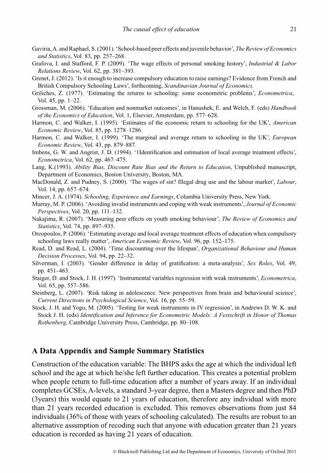
Construction of the education variable: The BHPS asks the age at which the individual leftschool and the age at which he/she left further education. This creates a potential problemwhen people return to full-time education after a number of years away. If an individualcompletes GCSEs, A-levels, a standard 3-year degree, then a Masters degree and then PhD(3years) this would equate to 21 years of education, therefore any individual with morethan 21 years recorded education is excluded. This removes observations from just 84individuals (36% of those with years of schooling calculated). The results are robust to analternative assumption of recoding such that anyone with education greater than 21 yearseducation is recorded as having 21 years of education.


22 BulletinTA

BL

EA

1

Sam

ple

sum

mar

yst

atis

tics

Var

iabl

eM

ean

SDM

inM

axV

aria

ble

Mea

nSD

Min

Max

Num

ber

ofob

serv

atio

nspe

rpe

rson

9.38

04.

516

115

Eth

nici

ty:O

ther

0.00

70.

083

01

Log

wag

e2.

214

0.43

70.

848

3.40

7Fa

ther

’soc

ccl

ass:

10.

139

0.34

60

1Y

ears

ofsc

hool

ing

12.5

072.

646

721

Fath

er’s

occ

clas

s:2

0.06

40.

244

01

Smok

erat

age

160.

315

0.46

50

1Fa

ther

’soc

ccl

ass:

30.

038

0.19

10

1In

imum

scho

olle

avin

gag

ew

as16

0.53

70.

499

01

Fath

er’s

occ

clas

s:4

0.04

90.

216

01

Age

39.9

9110

.757

1965

Fath

er’s

occ

clas

s:5

0.23

40.

423

01

Coh

ort:

born

inth

e19

20s

0.00

30.

052

01

Fath

er’s

occ

clas

s:6

0.04

40.

205

01

Coh

ort:

born

inth

e19

30s

0.05

00.

219

01

Fath

er’s

occ

clas

s:7

0.03

20.

177

01

Coh

ort:

born

inth

e19

40s

0.20

30.

402

01

Fath

er’s

occ

clas

s:8

0.17

10.

377

01

Coh

ort:

born

inth

e19

50s

0.27

40.

446

01

Fath

er’s

occ

clas

s:9

0.08

60.

280

01

Coh

ort:

born

inth

e19

60s

0.31

90.

466

01

Fath

er’s

occ

clas

s:10

0.14

30.

350

01

Coh

ort:

born

inth

e19

70s

0.14

60.

354

01

Mot

her’

soc

ccl

ass:

10.

037

0.18

80

1C

ohor

t:bo

rnin

the

1980

s0.

005

0.06

90

1M

othe

r’s

occ

clas

s:2

0.02

60.

159

01

Reg

ion:

Nor

th0.

068

0.25

20

1M

othe

r’s

occ

clas

s:3

0.03

20.

175

01

Reg

ion:

Yor

kshi

re0.

097

0.29

60

1M

othe

r’s

occ

clas

s:4

0.09

80.

297

01

Reg

ion:

Nor

thW

est

0.10

60.

308

01

Mot

her’

soc

ccl

ass:

50.

029

0.16

80

1R

egio

n:E

astM

idla

nds

0.09

20.

290

01

Mot

her’

soc

ccl

ass:

60.

073

0.26

00

1R

egio

n:W

estM

idla

nds

0.08

60.

280

01

Mot

her’

soc

ccl

ass:

70.

066

0.24

80

1R

egio

n:E

astA

nglia

0.04

30.

202

01

Mot

her’

soc

ccl

ass:

80.

051

0.22

00

1R

egio

n:So

uth

Eas

t0.

280

0.44

90

1M

othe

r’s

occ

clas

s:9

0.08

40.

277

01

Reg

ion:

Sout

hW

est

0.10

00.

300

01

Mot

her’

soc

ccl

ass:

100.

505

0.50

00

1R

egio

n:W

ales

0.05

10.

221

01

Nuc

lear

fam

ilyto

160.

831

0.37

50

1R

egio

n:Sc

otla

nd0.

076

0.26

50

1E

arly

1990

s0.

195

0.39

60

1E

thni

city

:Whi

te0.

974

0.16

00

1M

id19

90s

0.21

30.

409

01

Eth

nici

ty:B

lack

0.00

40.

062

01

Lat

e19

90s

0.22

10.

415

01

Eth

nici

ty:A

sian

0.01

60.

124

01

Post

2000

0.37

10.

483

01

Tota

lnum

ber

ofob

serv

atio

ns21

265

Not

es:

‘nuc

lear

fam

ily’

to16

mea

nsliv

edw

ithbo

thna

tura

lpa

rent

sfr

ombi

rth

toag

e16

.oc

cupa

tiona

lcl

ass

dum

mie

s:(1

)m

anag

emen

t,(2

)pr

ofes

sion

al,

(3)

asso

-ci

ate

prof

essi

onal

/tech

nica

l,(4

)cl

eric

al/s

ecre

tari

al,t

aken

and

the

mea

nre

sidu

alfo

rea

chin

divi

dual

isca

lcul

ated

.The

sear

eth

enra

nked

into

(5)

craf

tan

dre

late

d,(6

)pe

rson

al/p

rote

ctiv

ese

rvic

es,(

7)sa

les,

(8)

plan

t/mac

hine

oper

ativ

e,(9

)ot

her,

(10)

self

-em

p/un

emp.


The Causal Effect of Education on Wages Revisited

Documents

Transcript of The Causal Effect of Education on Wages Revisited