The Causal Effects of Competition onInnovation: Experimental Evidence

Working paper

Philippe Aghion∗, Stefan Bechtold†, Lea Cassar‡, and Holger Herz§

February 20, 2014

Abstract

In this paper, we design two laboratory experiments to analyze thecausal effects of competition on step-by-step innovation. Innovationsresult from costly R&D investments and move technology up one step.Competition is inversely measured by the ex post rents for firms thatoperate at the same technological level, i.e. for neck and neck firms.First, we find that increased competition leads to a significant increasein R&D investments by neck and neck firms. Second, increased com-petition decreases R&D investments by firms that are lagging behind,in particular if the time horizon is short. Third, we find that increasedcompetition affects industry composition by reducing the fraction ofsectors where firms are neck and neck. All these results are consistentwith the predictions of step-by-step innovation models.

∗Harvard University, paghion@fas.harvard.edu.†ETH Zurich, sbechtold@ethz.ch.‡University of Zurich, lea.cassar@econ.uzh.ch.§University of Zurich, holger.herz@econ.uzh.ch. We would like to thank Daniel Chen,

Ernst Fehr, Bernhard Ganglmair, Klaus Schmidt, Roberto Weber, as well as the partici-pants at the IMEBE 2013 conference and at the ETH Zurich/Max Planck Workshop onthe Law & Economics of Intellectual Property and Competition Law 2013 for their usefulcomments and feedback.

1

1 Introduction

The relationship between competition and innovation has long been of inter-est to economists and motivated numerous studies, both theoretical and em-pirical, over the past three decades (e.g., Hart (1980); Schmidt (1997); Aghionet al. (2001); Vives (2008); Schmutzler (2009, 2013) and Nickell (1996); Blun-dell et al. (1999); Aghion et al. (2005); Aghion and Griffith (2006)). However,the existing empirical studies on this subject face the issue that the relation-ship between competition and innovation is endogenous (Jaffe (2000); Halland Harhoff (2012)).1 Moreover, clean and direct measures of innovationand competition are usually not available in field data, which can lead to theadditional problem of measurement error.

To address these two issues head on, in this paper we employ the methodsof experimental economics to analyze the effects of competition on step-by-step innovation. The predictions we submit to our experiments are drawnfrom the step-by-step innovation models of Aghion et al. (1997, 2001) andAghion and Howitt (2009). These models predict that product market com-petition should foster innovation in neck-and-neck sectors where firms oper-ate at the same technological level: in such sectors, increased product marketcompetition reduces pre-innovation rents, thereby increasing the incremen-tal profits from innovating and becoming a leader. This is known as the“escape-competition effect”. On the other hand, these models predict a neg-ative “Schumpeterian effect”on laggard firms in unleveled sectors: increasedcompetition reduces the post-innovation rents of laggard firms and thus theirincentive to catch up with the leader. However, this effect is (partly) coun-teracted by an “anticipated escape-competition effect”once the laggard hascaught up with the current leader in the sector. The escape-competition andSchumpeterian effects, together with the fact that the equilibrium fraction ofneck-and-neck sectors depends positively on the laggards’ innovation incen-tives in unleveled sectors and negatively on neck-and-neck firms’ innovationincentives in leveled sectors, imply that the equilibrium fraction of sectorswhere firms are neck and neck should decrease with competition: this is the“composition effect”of competition.

To test these predictions, we design two laboratory experiments. In both

1See Blundell et al. (1999) and Aghion et al. (2005) for a discussion of the endogeneityissue and for attempts at addressing it. For various empirical approaches to identify causalrelationships between patenting activities and innovation, see Murray and Stern (2007);Williams (2013); Galasso and Schankerman (2013).

2

experiments, pairs of subjects are matched for a number of periods, forming asector. In each period, one of the two subjects can choose an R&D investmentwhich determines the probability of a successful innovation in that period.Innovation is costly and has an associated cost generated via a quadratic costfunction. If innovation is successful, the technological level of the innovativesubject increases by one step. At the end of each period, rents are distributedto each subject according to her relative technological location in her sector.If the two subjects are in an unleveled sector, then the subject ahead (the“leader”) receives a positive monopoly rent, whereas the other subject inthe same sector (the “laggard”) makes zero profit. If subjects in the samesector are neck and neck, their rents are equal and depend on the degree ofcompetition. In the no competition treatment, these firms are able to split themonopoly rent between them, whereas under the full competition treatmentthe neck-and-neck firms’ profits are zero. In the intermediate competitiontreatment, neck-and-neck subjects are able to split half the monopoly rentbetween them.

We conduct an “infinite horizon” experiment to bring out the escape-competition and the Schumpeterian effects most clearly and a “finite hori-zon” experiment to assess the composition effect. In the infinite horizon ex-periment, we exogenously vary the subjects’ (or “firms’”) starting positions.That is, some pairs of subjects start as unleveled sectors while other pairsstart as neck-and-neck sectors. This design feature, together with the treat-ment variation in the degree of competition, allows us to causally assess theescape-competition effect and the Schumpeterian effect. After every period,the interaction between two paired subjects ends with a positive stoppingprobability: in other words, the time horizon is infinite but we exogenouslyvary the expected time horizon across sessions. Pairs either faced a short timehorizon - a 80% probability of ending the game after each round– or a longtime horizon – a 10% probability of ending the game after each round. Thisset up allows us to test an additional prediction from the theory: We shouldexpect a more negative impact of competition on laggards’ innovation inten-sity in the short horizon treatment than in the long horizon treatment, sincethe longer the time horizon, the more the anticipated escape-competitioneffect may counteract the Schumpeterian effect.

In the finite horizon experiment, all subjects faced the same finite timehorizon of 50 periods. Each pair starts as a neck-and-neck sector, and theability to innovate alternates between the two subjects across periods. Be-

3

cause of the exogenous variation of competition across treatments, this de-sign allows us to cleanly identify the causal effect of competition on industrycomposition and also on aggregate innovation outcomes.

The results can be summarized as follows. First, an increase in compe-tition leads to a significant increase in R&D investments by neck-and-neckfirms. Second, an increase in competition decreases R&D investments bylaggard firms. Moreover, this Schumpeterian effect is significantly strongerthe shorter the time horizon. Third, increased competition affects industrycomposition by reducing the fraction of neck-and-neck sectors, and overall,competition increases aggregate innovation. All these results are consistentwith the predictions of the step-by-step innovation model.

This paper relates to several strands of literature. First, it contributesto an extensive theoretical industrial organization literature on competition,rent dissipation, and research and development (see Tirole (1988)), and tothe patent race literature (Harris and Vickers (1985a,b, 1987)). Second,it relates to the endogenous growth literature and more specifically to itsSchumpeterian growth branch (see Aghion et al. (2013)).

Third, the paper contributes to the existing empirical literature on therelationship between competition and innovation (see Nickell (1996), Blun-dell et al. (1999), Aghion et al. (2005); Aghion and Griffith (2006); Acemogluand Akcigit (2012)). Our laboratory setting and the investment game thatwe study are stylized, yet competition and the time horizon both vary exoge-nously and moreover R&D investments are directly observed. This in turnallows us to complement the existing field evidence by shedding further lighton the causal rather than correlational relationship between competition andinnovation.

Fourth, the paper contributes to an emerging experimental literature oncompetition and innovation.2 Our experimental study differs from this lit-

2Thus Isaac and Reynolds (1988) analyze the effects of competition and appropri-ability in simultaneous investment, one-period patent races. They show that per-capitainvestments are decreasing with the number of contestants, whereas the aggregate level ofinvestment increases. Darai et al. (2010) find similar results in a two-stage game in whichR&D investment choices are followed by product market competition. Moreover, in a two-stage game with cost-reducing investments followed by a differentiated Cournot duopoly,Sacco and Schmutzler (2011) find a U-shape relationship between competition and inno-vation, the former being defined as the degree of product differentiation. Finally, Suetensand Potters (2007) finds that tacit collusion is higher in Bertrand competition than inCournot competition. However, the study does not look at the effect of competition oninnovation.

4

erature in particular by focusing on an environment in which innovation iscumulative over time.3 And to our knowledge, we are the first to design a lab-oratory experiment to examine the escape competition and Schumpeterianeffects in a dynamic investment environment with different time horizons,and to assess the composition effect.

The remaining part of the paper is organized as follows. Section 2 laysout the basic step-by-step innovation model and derives its main predictions.Section 3 presents the setup for the two experiments. Section 4 outlays theresults, and Section 5 concludes.

2 Theoretical predictions

To motivate and guide our experiment, and to derive our main predictions,we first present a simple version of the model with step-by-step innovations.While we chose to write the simplest possible model for pedagogical purposes,the predictions derived in this Section are robust to generalizations of theenvironment (see, for example, Aghion et al. (2001)).

In this model, a “laggard firm”, i.e a firm that is currently behind thetechnological leader in the same sector must catch up with the leader be-fore becoming a leader itself. This step-by-step assumption implies that, ina positive fraction of sectors, firms will be neck and neck, i.e. at the sametechnology level. By making life more difficult for neck-and-neck firms, ahigher degree of product market competition will encourage them to inno-vate in order to acquire a significant lead over their rivals. However, highercompetition may have a discouraging effect on innovation by laggard firmsin unleveled sectors.

2.1 Basic environment

We consider a simple Schumpeterian growth model in continuous time. Thereis a continuous measure L of infinitely-lived individuals each of whom supplies

3Isaac and Reynolds (1992) also study innovation investments over time. However,the authors do not distinguish between the escape-competition and the Schumpeterianeffect, nor do they test the composition effect of competition. Similarly, Zizzo (2002) andBreitmoser et al. (2010) study innovation investments in a multi-stage patent race. Thesepapers, however, do not look at the effect of varying competition and therefore cannotaddress the Schumpeterian-, escape competition- and composition effects.

5

one unit of labor per unit of time. Each individual has intertemporal utility

ut =

∫ 1

0

lnCte−ρtdt

where

lnCt =

∫ 1

0

ln yjtdj,

and where each yj is the sum of two goods produced by (infinitely-lived)duopolists in sector j :

yj = yAj + yBj.

The logarithmic structure of the utility function implies that in equilib-rium individuals spend the same amount on each basket yj.

4 We choose thisexpenditure as the numeraire, so that a consumer chooses each yAj and yBjto maximize yAj +yBj subject to the budget constraint: pAjyAj +pBjyBj = 1;that is, she will devote the entire unit of expenditure to the least expensiveof the two goods.

2.1.1 Technology and innovation

Each firm takes the wage rate as given and produces using labor as the onlyinput according to the following linear production function,

yit = γkitlit, i ∈ {A,B}

where ljt is the labor employed, kit denote the technology level of duopolyfirm i at date t, and γ > 1 is a parameter that measures the size of a leading-edge innovation. Equivalently, it takes γ−ki units of labor for firm i to produceone unit of output. Thus the unit costs of production is simply ci = wγ−ki

which is independent of the quantity produced.

4To see this, note that a final good producer will choose the yj ’s to maximizeu =

∫ln yjdj subject to the budget constraint

∫pjyjdj = E, where E denotes current

expenditures. The first-order condition for this is:

∂u/∂yj = 1/yj = λpj for all j

where λ is a Lagrange multiplier. Together with the budget constraint this first-ordercondition implies

pjyj = 1/λ = E for all j.

6

An industry j is thus fully characterized by a pair of integers (kj,mj)where kj is the leader’s technology and mj is the technological gap betweenthe leader and the follower.5

For expositional simplicity, we assume that knowledge spillovers betweenthe two firms in any intermediate industry are such that neither firm can getmore than one technological level ahead of the other, that is:

m ≤ 1.

In other words, if a firm already one step ahead innovates, the lagging firmwill automatically learn to copy the leader’s previous technology and therebyremain only one step behind. Thus, at any point in time, there will betwo kinds of intermediate sectors in the economy: (i) level or neck-and-necksectors where both firms are at technological par with one another, and(ii) unleveled sectors, where one firm (the leader) lies one step ahead of itscompetitor (the laggard or follower) in the same industry.6

To complete the description of the model, we just need to specify theinnovation technology. Here we simply assume that by spending the R&Dcost ψ(z) = z2/2 in units of labor, a leader firm moves one technologicalstep ahead, with probability z. We call z the “ innovation rate” or “ R&Dintensity” of the firm. We assume that a laggard firm can move one stepahead with probability h, even if it spends nothing on R&D, by copying theleader’s technology. In other words, it is easier to reinvent the wheel than toinvent the wheel. Thus z2/2 is the R&D cost (in units of labor) of a laggardfirm moving ahead with probability z+h. Let z0 denote the R&D intensity ofeach firm in a neck-and-neck industry; and let z−1 denote the R&D intensityof a follower firm in an unleveled industry; if z1 denotes the R&D intensity ofthe leader in an unleveled industry, note that z1 = 0, since our assumption ofautomatic catch-up means that a leader cannot gain any further advantageby innovating.

5The above logarithmic final good technology together with the linear production coststructure for intermediate goods implies that the equilibrium profit flows of the leader andthe follower in an industry depends only upon the technological gap m between the twofirms (see Aghion and Howitt (1998, 2009)).

6See Aghion et al (2001) for an analysis of the more general case where there is no limitto the technological gap between leaders and laggards in unleveled sectors.

7

2.2 Equilibrium profits and competition in level andunleveled sectors

One can show that the equilibrium profits are as follows (see Aghion andHowitt (2009)). First, in an unleveled sector, the leader’s profit is equal to

π1 = 1− 1

γ,

whereas the laggard in the unleveled sector will be priced out of the marketand hence will earn a zero profit:

π−1 = 0

Consider now a level (or neck-and-neck) sector. If the two firms engagedin open price competition with no collusion, then Bertrand competition willbring (neck-an-neck) firms’ profits down to zero. At the other extreme, if thetwo firms collude so effectively as to maximize their joint profits and sharedthe proceeds, then they would together act like the leader in an unleveledsector, so that each firm will earn π1/2.

Now, if we model the degree of product market competition inversely bythe degree to which the two firms in a neck-and-neck industry are able tocollude, the normalized profit of a neck-and-neck firm will be of the form:

π0 = (1−∆) π1, 1/2 ≤ ∆ ≤ 1,

where ∆ parameterizes product market competition.

We next analyze how the equilibrium research intensities z0 and z−1 ofneck-and-neck and laggard firms respectively, vary with our measure of com-petition ∆.

2.3 The Schumpeterian and escape competition effects

Let Vm (resp. V−m) denote the normalized steady-state value of being cur-rently a leader (resp. a laggard) in an industry with technological gap m,and let w denote the steady-state wage rate. We have the following Bellman

8

equations:7

ρV0 = π0 + z0(V−1 − V0) + z0(V1 − V0)− wz20/2 (1)

ρV−1 = π−1 + (z−1 + h)(V0 − V−1)− wz2−1/2 (2)

ρV1 = π1 + (z−1 + h)(V0 − V1) (3)

where z0 denotes the R&D intensity of the other firm in a neck-and-neckindustry (we focus on a symmetric equilibrium where z0 = z0).

In words, the growth-adjusted annuity value ρV0 of currently being neck-and-neck is equal to the corresponding profit flow π0 plus the expected capitalgain z0(V1 − V0) of acquiring a lead over the rival plus the expected capitalloss z0(V−1−V0) if the rival innovates and thereby becomes the leader, minusthe R&D cost wz2

0/2. Similarly, the annuity value ρV1 of being a technologicalleader in an unleveled industry is equal to the current profit flow π1 plus theexpected capital loss z−1(V0 − V1) if the leader is being caught up by thelaggard (recall that a leader does not invest in R&D); finally, the annuityvalue ρV−1 of currently being a laggard in an unleveled industry, is equalto the corresponding profit flow π−1 plus the expected capital gain (z−1 +h)(V0 − V−1) of catching up with the leader, minus the R&D cost wz2

−1/2.

Using the fact that z0 maximizes the RHS of (1) and z−1 maximizes theRHS of (2), we have the first order conditions:

wz0 = V1 − V0 (4)

wz−1 = V0 − V−1. (5)

In Aghion, Harris and Vickers (1997) the model is closed by a labormarket clearing equation which determines ω as a function of the aggregatedemand for R&D plus the aggregate demand for manufacturing labor. Here,for simplicity we shall ignore that equation and take the wage rate w as given,normalizing it at w = 1.

Then, using (4) and (5) to eliminate the V ’s from the system of equations(1)-(3), we obtain a system of two equations in the two unknowns z0 and z−1 :

z20/2 + (ρ+ h)z0 − (π1 − π0) = 0 (6)

z2−1/2 + (ρ+ z0 + h)z−1 − (π0 − π−1)− z2

0/2 = 0 (7)

7Note that the left-hand-side of the Bellman equations should first be written as rV0−V̇0. Then, using the fact that on a balanced growth path V̇0 = gV0, and using the Eulerequation r − g = ρ, yields the Bellman equations in the text.

9

These equations can be solved recursively for unique positive values ofz0 and z−1, and we are mainly interested by how these are affected by anincrease in product market competition ∆. It is straightforward to see fromequation (6) and the fact that

π1 − π0 = ∆π1

that an increase in ∆ will increase the innovation intensity z0(∆) of a neck-and-neck firm. This is the escape competition effect:

Prediction 1 (Escape-competition effect): Innovation by neck and neckfirms is always stimulated by higher competition.

Because competition negatively affects pre-innovation rents, competitioninduces innovation in neck-and-neck sectors since firms are particularly at-tracted by the monopoly rent.

One can express z0(∆) as

z0(∆) = −(ρ+ h) +√

(ρ+ h)2 + 2∆π1

Taking the derivative

∂z0

∂∆=

π1√(ρ+ h)2 + 2∆π1

In particular, ∂z0∂∆

can be shown to decrease when the rate of time preferenceρ increases. This generates the next prediction:

Prediction 2 (Escape-competition effect by rate of time prefer-ence) The escape-competition effect is weaker for firms with high rate oftime preference.

In other words, patient neck-and-neck firms put more weight on the futurepost-innovation rents after having become a leader, and therefore, react morepositively to an increase in competition than impatient neck-and-neck firms.

Then, plugging z0(∆) into (7), we can look at the effect of an increasein competition ∆ on the innovation intensity z−1 of a laggard. This effectis ambiguous in general: in particular, for sufficiently high ρ, the effect isnegative as then z−1 varies like

π0 − π−1 = (1−∆)π1.

10

In this case the laggard is very impatient and thus looks at its short termnet profit flow if it catches up with the leader, which in turn decreases whencompetition increases. This is the Schumpeterian effect :

Prediction 3 (Schumpeterian effect): Innovation by laggard firms inunleveled sectors is discouraged by higher competition.

Since competition negatively affects the post-innovation rents of laggards,competition reduces innovation of laggards. However, for low values of ρ, thiseffect is counteracted by an anticipated escape competition effect :

Prediction 4 (Anticipated escape-competition effect): The effect ofcompetition on laggards’ innovation is less negative for firms with low rateof time preference.

In other words, patient laggards take into account their potential futurereincarnation as neck-and-neck firms, and therefore react less negatively toan increase in competition than impatient laggards. The lower the rate oftime preference, the stronger the (positive) anticipated escape-competitioneffect and therefore the more it mitigates the (negative) Schumpeterian effectof competition on laggards’ innovation incentives.

Thus the effect of competition on innovation depends on the situationin which a sector is. In unleveled sectors, the Schumpeterian effect is atwork even if it does not always dominate. But in level (or neck-and-neck)sectors, the escape-competition effect is the only effect at work; that is, morecompetition always induces neck-and-neck firms to innovate more in order toescape from tougher competition.

2.4 Composition effect

In steady state, the fraction of sectors µ1 that are unleveled is constant,as is the fraction µ0 = 1 − µ1 of sectors that are leveled. The fraction ofunleveled sectors that become leveled each period will be z−1 + h, so thesectors moving from unleveled to leveled represent the fraction (z−1 + h)µ1

of all sectors. Likewise, the fraction of all sectors moving in the oppositedirection is 2z0µ0, since each of the two neck-and-neck firms innovates withprobability z0. In steady state, the fraction of firms moving in one directionmust equal the fraction moving in the other direction:

(z−1 + h)µ1 = 2z0 (1− µ1) ,

11

which can be solved for the steady state fraction of unleveled sectors:

µ1 =2z0

z−1 + h+ 2z0

. (8)

This fraction is increasing in competition as measured by ∆ since ahigher ∆ increases R&D intensity 2z0 in neck-and-neck sectors (the escape-competition effect) whereas it tends to reduce R&D intensity z−1 + h inunleveled sectors (the Schumpeterian effect). This positive effect of compe-tition on the steady-state equilibrium fraction of neck-and-neck sectors werefer to as the composition effect of competition:

Prediction 5 (Composition effect): The higher the degree of compe-tition, the smaller the equilibrium fraction of neck-and-neck sectors in theeconomy.

More competition increases innovation incentives for neck-and-neck firmswhereas it reduces innovation incentives of laggard firms in unleveled sec-tors. Consequently this reduces the flow of sectors from unleveled to leveledwhereas it increases the flow of sectors from leveled to unleveled.

We now proceed to confront these predictions with experimental evidence.

3 The experiments

We conduct two separate experiments, the “infinite horizon” and the “finitehorizon” experiments, that are based on the same step-by-step innovationgame. The purpose of the infinite horizon experiment is to provide causalevidence for the escape-competition and Schumpeterian effects, both whenthe time horizon is long and when it is short. Exogenous variations in the timehorizon can equivalently be interpreted as exogenous variations in firms’ rateof time preference. The purpose of the finite horizon experiment is to observeduopolies over a long period of time in order to provide causal evidence forthe composition effect. We first present the basic features of our laboratorystep-by-step innovation game, and will then describe the specific features ofthe two experiments in more detail.

3.1 The step-by-step innovation game

At the center of our experimental design is a computerized step-by-step inno-vation game with the following features: Two subjects i and j are randomly

12

matched with each other, forming a sector. Before period 1, both subjectsare exogenously assigned to technology levels τ i and τ j. In each period, oneof the two subjects can choose an R&D investment n ∈ {0, 5, 10, . . . , 80},which determines the probability of a successful innovation in this period.8

Each subject is informed that the common quadratic R&D cost function isgiven by:

C(n) = 600

(n

100

)2

. (9)

At the beginning of period 1, it is randomly determined which subject caninvest in innovation in that period. If innovation is successful, the innovatormoves up one step from θ to θ+1. Thus, in our experiments only one subjectcould innovate at a time. This reduces the computational complexity of thegame by fixing subjects’ beliefs about their opponents’ current action andtherefore about the expected returns in that period from innovating. How-ever, precluding simultaneous moves in our experiment does not qualitativelyaffect the theoretical predictions of the model.9

To account for technology spillovers which may occur from leaders tolaggards, laggards are automatically granted with an additional innovationprobability of h = 30. Thus, the overall innovation probability is given byn+h, where n can be chosen from n ∈ {0, 5, 10, . . . , 50}, so that the maximalprobability of innovating is still given by n+ h = 80.

At the end of each period, payments are made to both subjects. Paymentsdepend on the technology levels θi and θj of subjects i and j. Payments afterevery period to subject i are determined by the following function:

πi =

200− C(n) if θi > θj(1−∆)200− C(n) if θi = θj0− C(n) if θi < θj.

8We have deliberately excluded the possibility to choose an investment in R&D of 100,i.e. to innovate with certainty. We believe that certain innovation would be an unrealisticfeature of the environment which we are studying.

9Indeed, while our experiments were conducted in discrete time, the model described inSection 2 is in continuous time. A continuous time implementation of the experiments wastechnically not feasible. Since the probability of simultaneous innovation is negligible whentime is continuous, alternating moves are in fact a closer experimental implementation ofthe continuous time model. Also note that Aghion and Howitt (2009) specify a step-by-step innovation model in which time is discrete, only one firm innovates in each period,and the basic theoretical predictions remain the same.

13

Subjects are symmetric, and payments to subject j are determined inexactly the same way. This profit function implies that the leader is alwaysable to earn a monopoly rent of 200 points. If subjects are neck and neck,their payoffs depend on the degree of competition in the sector, which ismeasured by ∆. If ∆ = 0.5, subjects are able to split the monopoly rentbetween them, whereas if ∆ = 1, subjects face perfect competition and rentsin neck-and-neck states are 0.10 Finally, if a subject is lagging behind hiscompetitor in terms of technology, her profit is 0. The costs associated withR&D are always subtracted from the rent earned.

After each period, each subject receives information about the behaviorof the other subject in the preceding period. In particular, she sees whichinvestment level the other subject has chosen, what the costs of innovationwere, whether the other subject benefited from a laggard innovation bonusof h = 30 in the preceding round, and whether she will benefit from a lag-gard innovation bonus in the current period. In addition, each subject seesthe payment of both subjects in the preceding period as well as the currenttechnology level and the overall income of both subjects over the entire treat-ment. Based on this information, subjects can decide how much to invest inthe current period.

3.2 The infinite horizon experiment

The infinite horizon experiment consisted of three different treatment vari-ations, some of which within subjects, and others across subjects. First, allsubjects participated in a full competition (∆ = 1) and in a no competitiontreatment (∆ = 0.5), which were played sequentially in varying order acrosssessions.

Second, each subject made decisions conditional on being a laggard orbeing neck-and-neck in the first round. I. e., the starting position was ran-domly varied within subject. In each treatment, it was randomly determined

10We chose to capture exogenous variations in the degree of competition by directlymodifying the payoffs to subjects in neck-and-neck states. In our view, this is the mostdirect and cleanest exogenous manipulation of competition in a step-by-step innovationmodel. An alternative approach in the experimental literature would be to vary thenumber of subjects competing in the same market. For the purposes of our experiments,however, we are less concerned by the particular channel whereby the competitive processaffects competitive outcomes, than by how the outcome of this competitive process affectsinnovation incentives.

14

whether both subjects were assigned to technology levels of τ i = 0, or whetherone of the subjects was given a head start and assigned to a technology levelof τ i = 1. If the sector was leveled at the start, it was randomly determinedwhich of the two firms could invest in the first round. If the sector was un-leveled, the subject that was randomly put into the laggard position couldinvest in the first period. We elicited the first round investment decisionsof all subjects using the strategy method. That is, we asked the subjectshow much they want to invest if they start in a neck-and-neck sector, andhow much they want to invest if they start as laggards. After choices weremade, the computer would randomly select the initial state of the sectorand which of the two firms could invest. The investment choice associatedwith the chosen state was then automatically implemented. The strategymethod was only used for first round investment choices. The exogenousvariation in competition and starting position allows us to causally test theescape-competition and Schumpeterian effects.

Third, the time horizon was varied across sessions. At the end of eachperiod, the game would end with a fixed and known stopping probabilityp. This procedure enables us to exogenously impose an infinite time horizonand exogenously vary the stopping probability p, which can be equivalentlyinterpreted as exogenous variation in the rate of time preference ρ. In somesessions subjects faced a short time horizon – 80% probability of ending thegame after each round– while in other sessions the subjects faced a long timehorizon – 10% probability of ending the game after each round. In the shorttime horizon treatment, a game lasted on average 2.2 rounds, whereas in thelong time horizon treatment, a game lasted on average 10 rounds. This designfeature allows us to test whether the escape-competition and Schumpeterianeffects vary conditional on the time horizon.

Table 3.2 summarizes the four treatment variations. Remember that ineach treatment, subjects made first period decisions conditional on being inthe laggard state and being in the neck-and-neck state.

Once the second period was entered into, the game progressed as follows:If a subject is lagging behind, that subject is given the right to invest.11 Ifthe sector is neck-and-neck, it is randomly determined at the beginning of theround which subject is able to invest. To make sure that subjects understoodthe experiment well, in particular the random stopping rule, they practiced

11This design feature is equivalent of the automatic catch-up assumption in the theory,that is, firms cannot be more than one technological level apart.

15

Time horizon

long (p = 0.1) short (p = 0.8)C

om

peti

tion

no comp.(∆ = 0.5)

long horizon /no competition

short horizon /no competition

full comp.(∆ = 1)

long horizon /full competition

short horizonfull competition

Table 1: Treatment variation: Infinite time horizon experiment

the game against a computer opponent for a period of 3 minutes before theexperiment started.12

The infinite horizon experiment is specifically designed to address the es-cape competition and the Schumpeterian effects. In order to obtain cleancausal evidence, exogenous assignment of subjects to neck-and-neck and lag-gard states in different competition and time horizon treatments is absolutelycrucial. Because subjects are only truly randomly assigned to the neck-and-neck or laggard state in the first period of the interaction, we restrict ourattention in the analysis to first period investments. To allow for some learn-ing, we repeated each competition treatment three times. So overall, eachsubject made six first-round investment decisions as a neck-and-neck firmand six first-round investment decisions as a laggard firm, three for eachcompetition treatment.

Once a game ends, subjects are re-matched with another subject whomthey have not been matched with previously. More specifically, we designedmatching groups and divided subjects within a matching group into a groupA and a group B. Each group A subject would only be matched with groupB subjects from the same matching group, but no subject would be matchedtwice with the same subject. 200 points were exchanged to SFr. 1 at theend of the experiment, and subjects were endowed with 5000 points at the

12They were informed that the computer’s investment decisions would be determinedrandomly, i. e., nothing could be learned from the computer’s strategy. If a game endedwithin the 3 minutes, they were informed about the final outcomes of that game and a newgame would start. This procedure allowed them to get familiar with the computer interfaceand in particular with the random stopping rule, so that they could form expectationsabout the length of the game.

16

beginning of the session, to ensure them against potential losses.

3.3 The finite horizon experiment

The finite horizon experiment involves three different competition treat-ments: No Competition (∆ = 0.5), Intermediate Competition (∆ = 0.75)and Full Competition (∆ = 1). We again employ a within subjects design,i.e., all subjects participate in all three treatments. This treatment variationis summarized in the table below:

Treatment CompetitionNo Competition ∆ = 0.5Intermediate Competition ∆ = 0.75Full Competition ∆ = 1

Table 2: Treatment variation: Finite time horizon experiment

Our main interest in the finite time horizon experiment is in analyzingpredictions that stem from the dynamics within sectors over an extendednumber of periods. An infinite time horizon would have yielded a largenumber of practical problems in terms of conducting the experiment as wellas in analyzing the data. The finite time horizon experiment consisted of 50periods in each treatment. To simulate an infinite game with expected timehorizon of 50 periods, the probability of ending the game after each periodwould have needed to be only 2%. This would have implied an expectedstandard deviation in treatment length of 50 periods. Consequently, thefinite time horizon experiment is better suited to address the causal effect ofcompetition on industry competition and aggregate innovation.

At the beginning of each treatment, all subjects are assigned to technol-ogy levels τ i = 0, i.e., all sectors start neck-and-neck. One subject is thenrandomly determined to invest in the first period. Thereafter, subjects alter-nate in their ability to invest. There was no automatic catch-up, i.e., subjectscould theoretically move more than one technological step apart from eachother. This is consistent with the most general version of the model pre-sented in Aghion et al. (2001) and generates the same predictions as simplerversions of the model.13

13See Aghion et al. (2001) for a generalization of the model in Section 2 which allowsfor more than one gap and derives similar results using calibrations. It is noteworthy,

17

To be ensured against potential losses, each subject was endowed with3000 points at the beginning of the first period. The exchange rate frompoints to SFr was 300:1.14 Subjects within a session are initially divided intogroup A and group B. In each treatment, a subject from group A is matchedwith a subject from group B. Between treatments, subjects are randomlyrematched with another subject from the other group whom they have notbeen matched with previously.

3.4 Experimental procedures

Between 18 and 22 subjects participated in each experimental session. Intotal, 4 experimental sessions of the infinite horizon experiment were con-ducted. To control for treatment order effects, each potential sequence of thetwo competition treatments was used in one session both for the long andfor the short time horizon. Moreover, 6 experimental sessions of the finitehorizon experiment were conducted. Again, to control for treatment ordereffects, sessions were designed such that each potential sequence of the threetreatments was used in one session.

The experiments were programmed and conducted with the software z-Tree (Fischbacher (2007)). All experimental sessions were conducted at theexperimental laboratory of the Swiss Federal Institute of Technology (ETH)in Zurich. Our subject pool consisted primarily of students at the Univer-sity of Zurich and ETH Zurich and were recruited using the ORSEE soft-ware (Greiner (2004)). The finite horizon experiment took place in February2012, and the infinite horizon experiment took place in December 2013. 118subjects participated in the finite horizon experiment, and 86 subjects par-ticipated in the infinite horizon experiment. Payment was determined by thesum of the final amounts of points a subject received in all treatments playedduring a session. In addition, each subject received a show-up fee of 10 SFr.On average, an experimental session lasted 1.5 hours. The average paymentin the finite horizon experiment was 45 SFr ($50.00), and 40.8 SFr ($44.7) inthe infinite horizon experiment.

however, that in about 80% of our experimental observations subjects are at most onetechnological gap apart from each other.

14Because the expected number of periods each subject plays in the finite and infiniteexperiments, the exchange rate was modified in order to provide subjects with appropriateearnings for participation in the experiments.

18

4 Results

In this section, we present our empirical results and compare them to theabove predictions. We will first discuss the effects of competition on R&Dinvestments in leveled and unleveled sectors by reporting the findings fromthe infinite horizon experiment. Thereafter, we will present the effects ofcompetition on industry composition as well as the overall effect of competi-tion on innovation outcomes resulting from the finite horizon experiment.

4.1 Evidence from the infinite horizon experiment

4.1.1 The escape-competition effect

Increased competition should have a positive effect on R&D investments iffirms are neck and neck. Empirically, we find in our experiment:

Result 1 (Escape-competition effect): An increase in competition leadsto a significant increase in R&D investments by neck-and-neck firms.

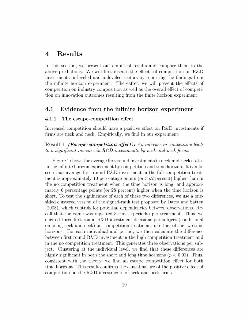
Figure 1 shows the average first round investments in neck-and-neck statesin the infinite horizon experiment by competition and time horizon. It can beseen that average first round R&D investment in the full competition treat-ment is approximately 10 percentage points (or 35.2 percent) higher than inthe no competition treatment when the time horizon is long, and approxi-mately 6 percentage points (or 28 percent) higher when the time horizon isshort. To test the significance of each of these two differences, we use a one-sided clustered version of the signed-rank test proposed by Datta and Satten(2008), which controls for potential dependencies between observations. Re-call that the game was repeated 3 times (periods) per treatment. Thus, weelicited three first round R&D investment decisions per subject (conditionalon being neck-and neck) per competition treatment, in either of the two timehorizons. For each individual and period, we then calculate the differencebetween first round R&D investment in the high competition treatment andin the no competition treatment. This generates three observations per sub-ject. Clustering at the individual level, we find that these differences arehighly significant in both the short and long time horizons (p < 0.01). Thus,consistent with the theory, we find an escape competition effect for bothtime horizons. This result confirms the causal nature of the positive effect ofcompetition on the R&D investments of neck-and-neck firms.

19

1520

2530

3540

45

Inve

stm

ents

in R

&D

no competition full competition

Long Time Horizon

1520

2530

3540

45

Inve

stm

ents

in R

&D

no competition full competition

Short Time Horizon

Figure 1: Average R&D investments in neck-and-neck industriesAverages are calculated using the average individual first round investmentsin neck-and-neck states in each treatment. The bars display one standarddeviation of the mean.

Furthermore, we can test if the size of the escape-competition effect varieswith the time horizon. According to the theory, the escape competition effectshould be stronger in the long time horizon than in the short time horizon.To test this prediction, we compare the differences in first round R&D in-vestments across competition treatments, as defined above, between subjectsthat participated in the short horizon treatment and subjects that partici-pated in the long horizon treatment, using the one-sided clustered versionof the rank-sum test proposed by Datta and Satten (2005). While we doobserve a larger effect of competition on investment in the long time horizonthan in the short time horizon (10 versus 6 percentage points), clustering atthe individual level, we find that this difference is not statistically significant(p = 0.26).

Result 2 (Escape-competition effect and time horizon): We find nosignificant difference in the escape competition effect between the short timehorizon and the long time horizon.

Similar results are found by running OLS regressions, which are reportedin Table 3. It can be seen that the escape-competition effect is very ro-bust across different regression specifications. More specifically, average first

20

round investments in the full competition treatment are between 6 and 8 per-centage points higher than average first round investments in the no compe-tition treatment, and the difference is highly significant. This holds whetherwe use all first round observations, or whether we restrict our analysis tothe third repetition only, after some learning has taken place. Finally, noticethat the coefficient of the interaction term of competition and time horizonis large and positive in all regression specifications. However, we cannotestablish significance.

Table 3: Investments in Round 1 Neck-and-Neck

(1) (2) (3)full comp 8.139*** 6.148** 6.729**

(2.091) (2.340) (2.917)long horizon 9.005*** 7.060** 9.880**

(2.766) (3.443) (3.774)full comp*long horizon 3.890 5.316

(4.117) (4.888)Constant 21.243*** 22.216*** 21.462***

(2.500) (2.481) (3.027)Adj. R2 0.097 0.098 0.148Observations 516 516 172

Standard errors are clustered at the individual level. Regressions (1) and (2) consider allrepetitions. Regression (3) only considers the third repetition. Treatment order fixed ef-fects and repetition fixed effects (only in regressions (1) and (2)) are included. Significancelevels: *** p<.01, ** p<.05, * p<.1.

4.1.2 The Schumpeterian and anticipated escape-competition ef-fects

Increased competition is expected to have a negative effect on R&D invest-ments if firms are lagging behind. Empirically, we find in our experiments:

Result 3 (Schumpeterian effect): An increase in competition decreasesR&D investments of laggards.

Figure 2 shows the average first round investments of laggard firms in un-leveled states in the infinite time horizon experiment, divided by competitionand time horizon. It can be seen that average first round R&D investments

21

in the full competition treatment is approximately 6 percentage points (or20 percent) lower than in the no competition treatment when the time hori-zon is long, and approximately 11 percentage points (or 42.3 percent) lowerwhen the time horizon is short. To test the significance of each of these twodifferences, we again use the one-sided clustered version of the signed-ranktest proposed by Datta and Satten (2008). As for the neck-and-neck case,we collected three first round R&D investment decisions per subject (condi-tional on being a laggard) per competition treatment, in either of the twotime horizons. For each individual and period, we then calculate the differ-ence between first round R&D investment in the high competition treatmentand in the no competition treatment. This generates three observations persubject. Clustering at the individual level, we find that these differencesare highly significant in both the short and long time horizons (p < 0.01).Thus, consistent with the theory, we find evidence of a Schumpeterian effectin unleveled sectors.

1015

2025

3035

Inve

stm

ents

in R

&D

no competition full competition

Long Time Horizon

1015

2025

3035

Inve

stm

ents

in R

&D

no competition full competition

Short Time Horizon

Figure 2: Average R&D investments of laggards in unleveled in-dustries Averages are calculated using the average individual first roundinvestments of laggards in unleveled states in each treatment. The bars dis-play one standard deviation of the mean.

Furthermore, by comparing the effect of competition on laggards’ invest-ment across time horizons, we find:

Result 4 (Anticipated escape-competition effect): The Schumpete-

22

rian effect is stronger the shorter a firm’s time horizon.

According to the theory, the Schumpeterian effect should decrease as thetime horizon increases. To test this prediction, we compare the differencesin first round R&D investments across competition treatments, as definedabove, between subjects that participated in the short horizon treatmentand subjects that participated in the long horizon treatment, again using theone-sided clustered version of the rank-sum test (Datta and Satten (2005)).Clustering at the individual level, we find that this difference is statisticallysignificant (p = 0.02).

Similar results are found by running OLS regressions. These are reportedin Table 4. Average first round investments in the full competition treatmentare between 10 and 13 percentage points lower than average first round in-vestments in the no competition treatment, when the time horizon is short.Consistent with the theory, when the time horizon is long, the Schumpeterianeffect is less pronounced by approximately 4.8 to 5.5 percentage points, asreflected in the statistical significance of the interaction term in regressions(2) and (3). This significance is, however, only marginal (p < 0.1).

Table 4: Laggard Investments

(1) (2) (3)full comp –8.170*** –10.621*** –12.902***

(1.474) (1.686) (1.909)long horizon 6.232*** 3.838 3.067

(2.122) (2.440) (2.779)full comp*long horizon 4.788* 5.516*

(2.864) (3.256)Constant 25.414*** 26.611*** 26.576***

(1.761) (1.753) (2.037)Adj. R2 0.113 0.117 0.136Observations 516 516 172

Standard errors are clustered at the individual level. Regressions (1) and (2) consider allrepetitions. Regression (3) only considers the third repetition. Treatment order fixed ef-fects and repetition fixed effects (only in regressions (1) and (2)) are included. Significancelevels: *** p<.01, ** p<.05, * p<.1.

23

.3

.35

.4

.45

.5

.55

Fre

quen

cy

nocompetition

intermediatecompetition

fullcompetition

Figure 3: Average frequency of neck-and-neck states. The frequency ofneck-and-neck states in a sector over 50 periods constitutes one observation.The bars display one standard deviation of the mean.

4.2 Evidence from the finite horizon experiment

4.2.1 The composition effect

The exogenous variation of competition across treatments in the finite hori-zon experiment allows us to also identify the causal effect of competition onindustry composition as well as on aggregate innovation outcomes.

According to the theory, we should observe a larger fraction of sectorsbeing neck-and-neck the smaller the degree of competition. This is indeedwhat we find and is summarized below.15

Result 5 (Composition effect): As competition increases, sectors be-come less likely to be neck and neck, and subjects are more likely to be tech-nologically apart from each other.

Evidence for the composition effect can be seen in Figure 3, which showsthe average fraction of periods in which sectors were neck and neck, condi-tional on the degree of competition. As the Figure shows, the frequency of

15Remember that a sector is equal to one duopoly in the experiment, formed by twosubjects.

24

observing leveled sectors decreases by approximately 5 percentage points asthe degree of competition in the industry increases by 0.25.

Table 5: Composition effect

(1)∆ –0.205 ***

(0.044)Constant 0.588 ***

(0.075)Adj. R2 0.019Observations 177

A sector in a competition treatment accounts for one observation in these regressions.Regression (1) uses the frequency of neck-and-neck states in a sector during the 50 periodsas the outcome variable. Treatment order fixed effects are included. Standard errors areclustered on the session level. Significance levels: *** p < .01, ** p < .05, * p < .1.

To assess the statistical significance of these effects, we compare the fre-quency of neck-and-neck states in a sector across the different competitiontreatments using regression analysis. The dependent variable is the fractionof observed neck-and-neck states within a sector. The regression includestreatment-order fixed effects, and standard errors are clustered on the ses-sion level. Results are shown in Table 5. We find that when our competitionmeasure increases by 0.25, the relative frequency of sectors being neck andneck decreases by 5.1 percentage points, and this decrease is highly signifi-cant.

4.2.2 The effect of competition on aggregate outcomes

Next, we can look at the effect of competition on aggregate R&D investmentsin our finite horizon experiment.

Result 6 (Aggregate innovation): Competition increases average R&Dinvestments and, as a result, the average level of technology that is ultimatelyreached in a sector in our experiment.

Figure 4 shows the average final technology level of the leading firm withina sector across competition treatments. The figure shows that the averagefinal technology level of the leading firm increases by 0.5 points, from 11.7

25

10

11

12

13

14

nocompetition

intermediatecompetition

fullcompetition

Figure 4: Average technology level reached within a sector. Themaximum level of technology reached in a sector over 50 periods constitutesone observation. The bars display one standard deviation of the mean.

to 12.2, when competition increases from no competition to intermediatecompetition. The average final technology level increases by another 1.4points to 13.5 when competition increases to full competition. Again, we canevaluate the statistical significance of these effects using regression analysis.The regression includes treatment order fixed effects, and standard errors areclustered on the session level. Results are shown in Table 6.

Column (1) in Table 6 provides strong empirical support for Result 6.As ∆ increases by 0.25 points, the final technology level of the leading firmincreases by 0.9 points, and this increase is significant. Column (2) in Ta-ble 6 shows results from a regression of R&D investments on the degree ofcompetition. This regression uses all observations, and besides individualfixed effects and treatment order fixed effects, no controls are included in theregression specification. Therefore, the coefficient on ∆ can be interpretedas the average effect of competition on R&D investments over the course ofour 50 round experiment. It can be seen that R&D investments on averageincrease by 3 percentage points (roughly 10 percent) as ∆ increases by 0.25points.

Hence, our setup provides evidence of a positive impact of competition onR&D investments as well as on the maximal technology level reached withina sector.

26

Table 6: Overall technological progress

(1) (2)Max. Tech. Level Avg. R&D Investment

∆ 3.597** 11.926***(1.124) (3.821)

Constant 9.812*** 28.300***(1.243) (3.156)

Adj. R2 0.007 0.012Observations 177 8850

A sector in a competition treatment accounts for one observation in these regressions.Regression (1) uses the maximum final technology level in a sector as the outcome variable.Regression (2) uses all individual R&D investment choices as observations. Treatmentorder fixed effects and individual fixed effects are included. Standard errors are clusteredon the session level. Significance levels: *** p < .01, ** p < .05, * p < .1.

5 Conclusion

In this paper, we provided a first attempt at analyzing the effect of compe-tition on step-by-step innovation in the laboratory. Using the lab instead offield data has several advantages. First, it addresses the endogeneity issuehead on: our results do capture causal effects of competition on innovationincentives. Second, the lab experiment allows us to disentangle the effectsof competition on innovation in leveled and unleveled sectors. In particu-lar, we find strong evidence of an escape-competition effect in neck-and-necksectors. Third, our design allows us to study how the effect of competitionon innovation varies with the time horizon. Consistent with theory, we showthat the Schumpeterian effect is stronger in the short horizon treatment thanin long horizon treatment, suggesting that in the latter case, an anticipatedescape-competition effect is also at work. Fourth, we are able to identifythe causal effect of competition on industry composition and on aggregateoutcomes. We find that, as competition increases, sectors become less likelyto be neck and neck, and the average technology level of the leading firmincreases.

The methodology used in the paper can be used to sort out other open de-bates in industrial organization and law & economics. For example, one could

27

use experiments to study the effects of patent protection or R&D subsidies,16

or the relative performance of various intellectual property legislations or theimpact of various antitrust policies,17 or the effects of various contractual orinstitutional arrangements, on innovation and entry. The industrial organi-zation and law & economics literatures often point to counteracting effectswithout always spelling out the circumstances under which one particulareffect should be expected to dominate. We believe that lab experiments canfill this gap by providing more precise predictions as to when such or sucheffect should indeed dominate. This and other extensions of our analysis inthis paper are left to future research.

16In Acemoglu and Akcigit (2012), this corresponds to our parameter h.17Experimental testing may be particularly interesting given the low variance of intel-

lectual property regimes across countries which results from international harmonizationefforts.

28

References

Acemoglu, D. and U. Akcigit (2012). Intellectual Property Rights: Policy,Competition and Innovation. Journal of the European Economic Associa-tion 10, 1–42.

Aghion, P., U. Akcigit, and P. Howitt (2013). What Do We Learn FromSchumpeterian Growth Theory? Working Paper 18824, National Bureauof Economic Research.

Aghion, P., N. Bloom, R. Blundell, R. Griffith, and P. Howitt (2005). Com-petition and Innovation: an Inverted-U Relationship. Quarterly Journalof Economics 120, 701–728.

Aghion, P. and R. Griffith (2006). Competition and Growth: ReconcilingTheory and Evidence. MIT Press.

Aghion, P., C. Harris, P. Howitt, and J. Vickers (2001). Competition, Im-itation and Growth with Step-by-Step Innovation. Review of EconomicStudies 68, 467–492.

Aghion, P., C. Harris, and J. Vickers (1997). Competition and Growth withStep-by-Step Innovation: An Example. European Economic Review 41,771–782.

Aghion, P. and P. Howitt (2009). The Economics of Growth. MIT Press.

Blundell, R., R. Griffith, and J. V. Reenen (1999). Market Share, MarketValue and Innovation in a Panel of British Manufacturing Firms. Reviewof Economic Studies 66, 529–554.

Breitmoser, Y., J. H. Tan, and D. J. Zizzo (2010). Understanding perpetualR&D races. Economic Theory 44 (3), 445–467.

Darai, D., D. Sacco, and A. Schmutzler (2010). Competition and Innovation:an Experimental Investigation. Experimental Economics 13, 439–460.

Datta, S. and G. Satten (2005). Rank-sum tests for clustered data. Journalof the American Statistical Association 471 (1), 908–915.

Datta, S. and G. Satten (2008). A signed-rank test for clustered data. Bio-metrics 64 (2), 501–507.

29

Fischbacher, U. (2007). z-Tree: Zurich Toolbox for Ready-made EconomicExperiments. Experimental Economics 10, 171–178.

Galasso, A. and M. A. Schankerman (2013). Patents andCumulative Innovation: Causal Evidence from the Courts.http://ssrn.com/abstract=2247011.

Greiner, B. (2004). The Online Recruitment System ORSEE: A Guide for theOrganization of Experiments in Economics. Discussion Papers on StrategicInteraction 2003–10, Max Planck Institute of Economics, Strategic Inter-action Group.

Hall, B. H. and D. Harhoff (2012). Recent Research on the Economics ofPatents. Annual Review of Economics 4, 541–565.

Harris, C. and J. Vickers (1985a). Patent Races and the Persistence ofMonopoly. Journal of Industrial Economics 33, 461–481.

Harris, C. and J. Vickers (1985b). Perfect Equilibrium in a Model of a Race.Review of Economic Studies 52, 193–209.

Harris, C. and J. Vickers (1987). Racing with Uncertainty. Review of Eco-nomic Studies 54, 1–21.

Hart, O. D. (1980). Perfect Competition and Optimal Product Differentia-tion. Journal of Economic Theory 22, 279–312.

Isaac, R. M. and S. S. Reynolds (1988). Appropriability and Market Structurein a Stochastic Invention Model. Quarterly Journal of Economics 103,647–671.

Isaac, R. M. and S. S. Reynolds (1992). Schumpeterian Competition inExperimental Markets. Journal of Economic Behavior & Organization 17,59–100.

Jaffe, A. B. (2000). The U.S. Patent System in Transition: Policy Innovationand the Innovation Process. Research Policy 29, 531–557.

Murray, F. and S. Stern (2007). Do Formal Intellectual Property RightsHinder the Free Flow of Scientific Knowledge?: An Empirical Test of theAnti-commons Hypothesis. Journal of Economic Behavior & Organiza-tion 63, 648–687.

30

Nickell, S. J. (1996). Competition and Corporate Performance. Journal ofPolitical Economy 104, 724–746.

Sacco, D. and A. Schmutzler (2011). Is There a U-shaped Relation BetweenCompetition and Investment? International Journal of Industrial Organi-zation 29, 65–73.

Schmidt, K. M. (1997). Managerial Incentives and Product Market Compe-tition. Review of Economic Studies 64, 191–214.

Schmutzler, A. (2009). Is Competition Good for Innovation? A SimpleApproach to an Unresolved Question. Foundations and Trends in Microe-conomics 5 (6), 355–428.

Schmutzler, A. (2013). Competition and investmenta unified approach. In-ternational Journal of Industrial Organization 31 (5), 477–487.

Suetens, S. and J. Potters (2007). Bertrand colludes more than Cournot.Experimental Economics 10 (1), 71–77.

Tirole, J. (1988). The Theory of Industrial Organization. MIT Press.

Vives, X. (2008). Innovation and Competitive Pressure. Journal of IndustrialEconomics 56, 419–469.

Williams, H. (2013). Intellectual Property Rights and Innovation: Evidencefrom the Human Genome. Journal of Political Economy 121, 1–27.

Zizzo, D. J. (2002). Racing with uncertainty: a patent race experiment.International Journal of Industrial Organization 20 (6), 877 – 902.

31