Investing in an Overvalued Market and Tail-Risk Hedging Michael Ning PhaseCapital

Michael DePalma PhaseCapital

Investing in an Overvalued Market and Tail-Risk HedgingQuarter 3 • 2017

37

The Case for Tail Hedging

Since the great recession officially ended in June 2009, risk has been rewarded and many risk assets have become very expensive in the process. The US central bank’s vast financial engineering effort has created excessive liquidity in the banking system that, in turn, fueled asset bubbles. According to Citi, “eight years into the cycle—and one where QE has been the asset market driver—virtually every market appears rich” (Citi Research— Asset Allocation, 25 May 2017). Minutes from a Federal Reserve meeting indicate some members of the central bank opined that equity markets were significantly overvalued. When measured by the Shiller PE Ratio (also known as the Cyclically Adjusted PE (CAPE) Ratio), an indicator based on average inflation-adjusted earnings from the previous 10 years, current US equity market valuation is as high as pre-Great Depression 1929 and is exceeded only by the 2000 technology bubble. Despite

some flaws, the Shiller PE Ratio is considered a better measurement of market valuation than typical formulations of the PE ratio because it eliminates ratio fluctuations that result from variations in profit margins during business cycles.

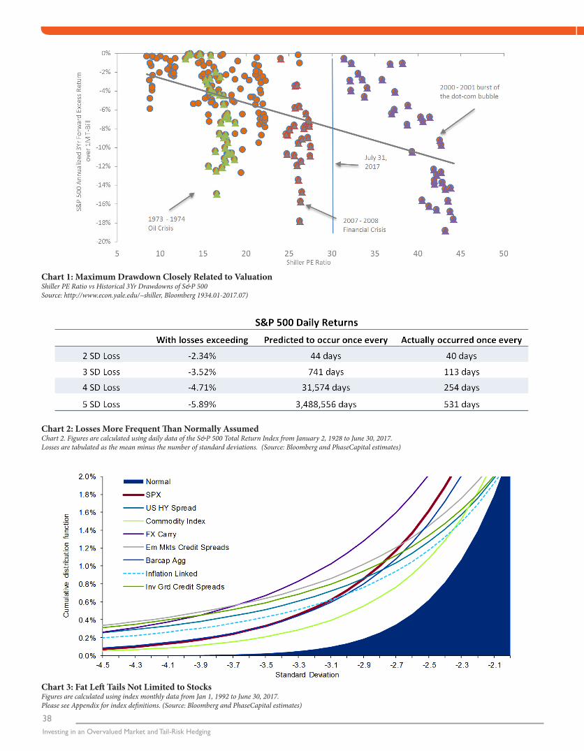
In Chart1 on the next page, we plot all the observations where the 3-year forward return on the S&P 500 is lower than 1-month T-Bill since 1934 against the starting level of the Shiller PE ratio when the downturn begins. The chart indicates that the maximum peak-to-trough loss of each bear market cycle is closely related to the level of market valuation.

A collapse of financial assets always threatens the real economy, its production, jobs, and price stability, and the ensuing ripple effects infer the existence of “tail risks.” The notion of tail risk refers to the “tail” associated with a normal distribution of returns. Under normal market conditions, asset returns are clustered

38Investing in an Overvalued Market and Tail-Risk Hedging

Chart 1: Maximum Drawdown Closely Related to Valuation Shiller PE Ratio vs Historical 3Yr Drawdowns of S&P 500 Source: http://www.econ.yale.edu/~shiller, Bloomberg 1934.01-2017.07)

Chart 2: Losses More Frequent Than Normally Assumed Chart 2. Figures are calculated using daily data of the S&P 500 Total Return Index from January 2, 1928 to June 30, 2017. Losses are tabulated as the mean minus the number of standard deviations. (Source: Bloomberg and PhaseCapital estimates)

Chart 3: Fat Left Tails Not Limited to Stocks Figures are calculated using index monthly data from Jan 1, 1992 to June 30, 2017. Please see Appendix for index definitions. (Source: Bloomberg and PhaseCapital estimates)

Investing in an Overvalued Market and Tail-Risk HedgingQuarter 3 • 2017

39

around the average, and the chance that some fall well beyond the average follows statistical laws. Tail risk is a form of portfolio risk that arises when the possibility that an investment will move more than some extreme threshold, say three standard deviations from the mean, is greater than what is implied by a normal distribution. Tail risk defined this way includes both extreme positive and negative outcomes. In practice, risk should be viewed in the context of all outliers; however, for the balance of this paper we focus on negative outcomes, or left-tail events. The idea of buying protection against such a rare occurrence seems counter-intuitive, but history shows that real-world returns have not always behaved like a normal distribution. Left-tail events, with extreme drawdowns and volatility, occur more frequently than assumed using traditional models of risk and asset allocation. This is illustrated in Chart 2 by the pattern of daily returns for the S&P 500 since 1928. In a normal distribution, a three standard deviation loss should have occurred on about 28 days since 1928 (or once every 741 days). In reality, extremes losses occurred about seven times more often—on 198 days (approximately once every 113 days).

Not just limited to stocks, as can be seen in Chart 3, almost all asset classes exhibit fatter tails than implied by a normal distribution:

Large drawdowns impede compounding and can result in failure to achieve portfolio return targets. Since taking tail risk may not be compensated, tail risk is a “non-core” risk for most investors with limited ability to withstand market shock. In particular, this type of uncertainty is not welcomed by investors whose return path is critical, such as underfunded pensions. Given this backdrop and these fears, tail-risk hedging—or protecting investment portfolios against extreme negative moves in the market—has been a frequent topic of conversation among market participants in recent years.

Chart 4: Volatility at Extreme Lows across Figures are calculated using index monthly data from Jan 1, 1998 to June 30, 2017. Please see Appendix for index definitions. (Source: Bloomberg and PhaseCapital estimates)

Tail-Risk Hedging Strategies

There are many ways to approach tail-risk hedging, ranging from the orthodox purchasing of “insurance” via put options to constructing a portfolio of volatility-focused strategies.

A simple purchase of put options can span multiple asset classes, e.g. S&P 500 put, VIX call, receiver on US 10YR Rates, CDX Index payer, and put options on high beta currencies. While the buyer of an option gets a hedge, the seller requires a risk premium to compensate for the risk transfer. The value of an option is driven by price movements of the underlying asset and its volatility, among other things. A fall in asset prices or a rise in volatility would increase the value of the option; likewise, when volatility is low, options often trade at relatively lower prices.

Despite rich equity valuations, equity indices have reached repeated records since the US presidential election and volatility across a broad spectrum of asset classes is at or near the lowest levels in decades according to data compiled by Bloomberg (Chart 4). For example, one-month implied volatility on Treasuries (the MOVE Index) fell to the lowest level on record. In more pronounced fashion, the CBOE Volatility Index, or VIX, closed below 10 on ten straight sessions in July. Since its price history began in 1990, 17 of the 26 days on which the VIX Index closed below 10 occurred in 2017.

Today’s overstretched asset prices and low volatility should mean historic opportunities to buy options. However, this traditional hedging strategy can still be expensive and may have limited benefit, even when tail events occur.

First, an option has a time-value component, becoming less valuable as it approaches expiration. This decay accelerates as the contract gets closer to expiration. Furthermore, options with different tenors often have different implied volatilities. While the spot VIX index hits record lows, VIX futures contracts expiring in 2018—a way to bet on where the VIX will be over the next

40Investing in an Overvalued Market and Tail-Risk Hedging

year—are at prices much closer to historically normal levels. When implied volatility curves are so steep—a condition known as being in “contango” where long-dated volatility is higher than short-dated volatility the decay in option value will proceed at an even higher rate.

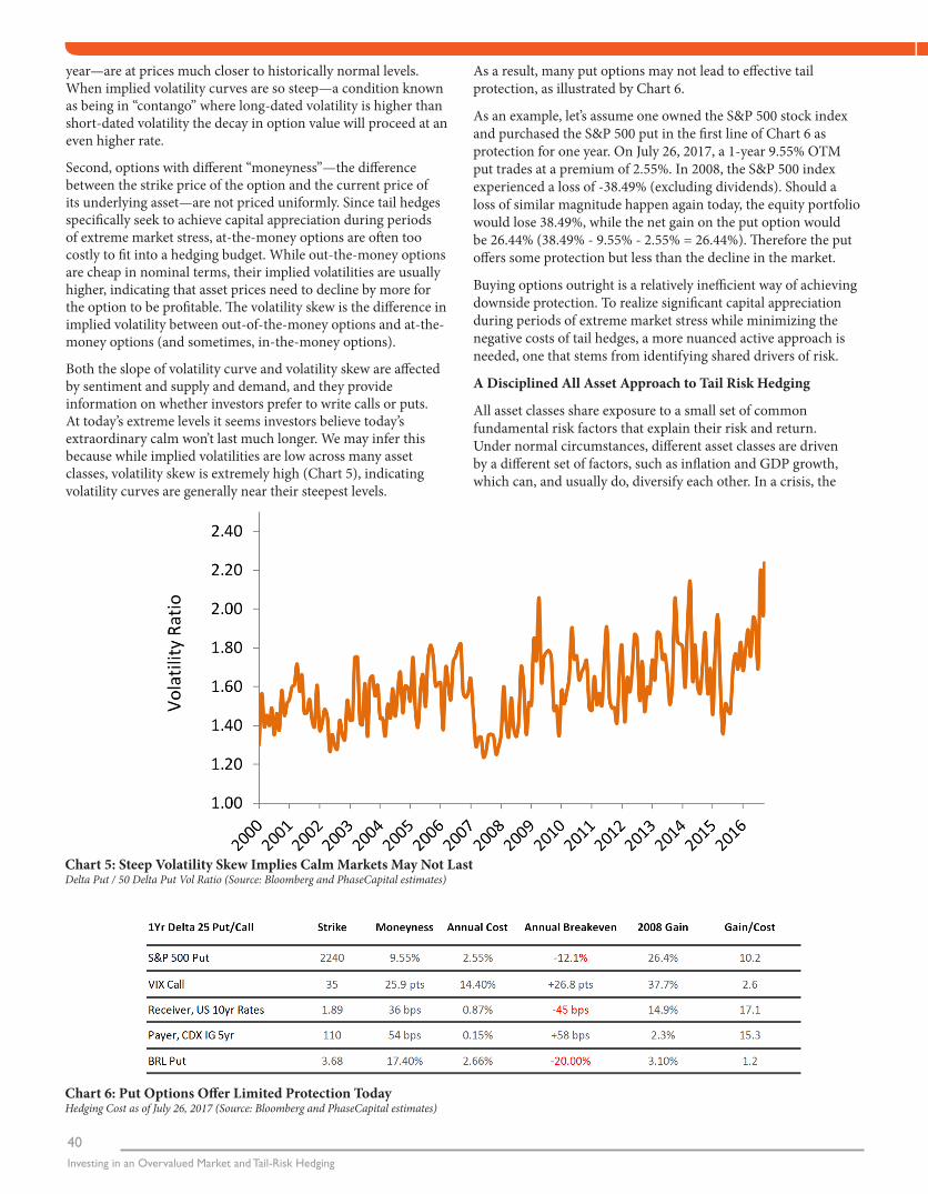
Second, options with different “moneyness”—the difference between the strike price of the option and the current price of its underlying asset—are not priced uniformly. Since tail hedges specifically seek to achieve capital appreciation during periods of extreme market stress, at-the-money options are often too costly to fit into a hedging budget. While out-the-money options are cheap in nominal terms, their implied volatilities are usually higher, indicating that asset prices need to decline by more for the option to be profitable. The volatility skew is the difference in implied volatility between out-of-the-money options and at-the-money options (and sometimes, in-the-money options).

Both the slope of volatility curve and volatility skew are affected by sentiment and supply and demand, and they provide information on whether investors prefer to write calls or puts. At today’s extreme levels it seems investors believe today’s extraordinary calm won’t last much longer. We may infer this because while implied volatilities are low across many asset classes, volatility skew is extremely high (Chart 5), indicating volatility curves are generally near their steepest levels.

Chart 5: Steep Volatility Skew Implies Calm Markets May Not Last Delta Put / 50 Delta Put Vol Ratio (Source: Bloomberg and PhaseCapital estimates)

Chart 6: Put Options Offer Limited Protection Today Hedging Cost as of July 26, 2017 (Source: Bloomberg and PhaseCapital estimates)

As a result, many put options may not lead to effective tail protection, as illustrated by Chart 6.

As an example, let’s assume one owned the S&P 500 stock index and purchased the S&P 500 put in the first line of Chart 6 as protection for one year. On July 26, 2017, a 1-year 9.55% OTM put trades at a premium of 2.55%. In 2008, the S&P 500 index experienced a loss of -38.49% (excluding dividends). Should a loss of similar magnitude happen again today, the equity portfolio would lose 38.49%, while the net gain on the put option would be 26.44% (38.49% - 9.55% - 2.55% = 26.44%). Therefore the put offers some protection but less than the decline in the market.

Buying options outright is a relatively inefficient way of achieving downside protection. To realize significant capital appreciation during periods of extreme market stress while minimizing the negative costs of tail hedges, a more nuanced active approach is needed, one that stems from identifying shared drivers of risk.

A Disciplined All Asset Approach to Tail Risk Hedging

All asset classes share exposure to a small set of common fundamental risk factors that explain their risk and return. Under normal circumstances, different asset classes are driven by a different set of factors, such as inflation and GDP growth, which can, and usually do, diversify each other. In a crisis, the

Investing in an Overvalued Market and Tail-Risk HedgingQuarter 3 • 2017

41

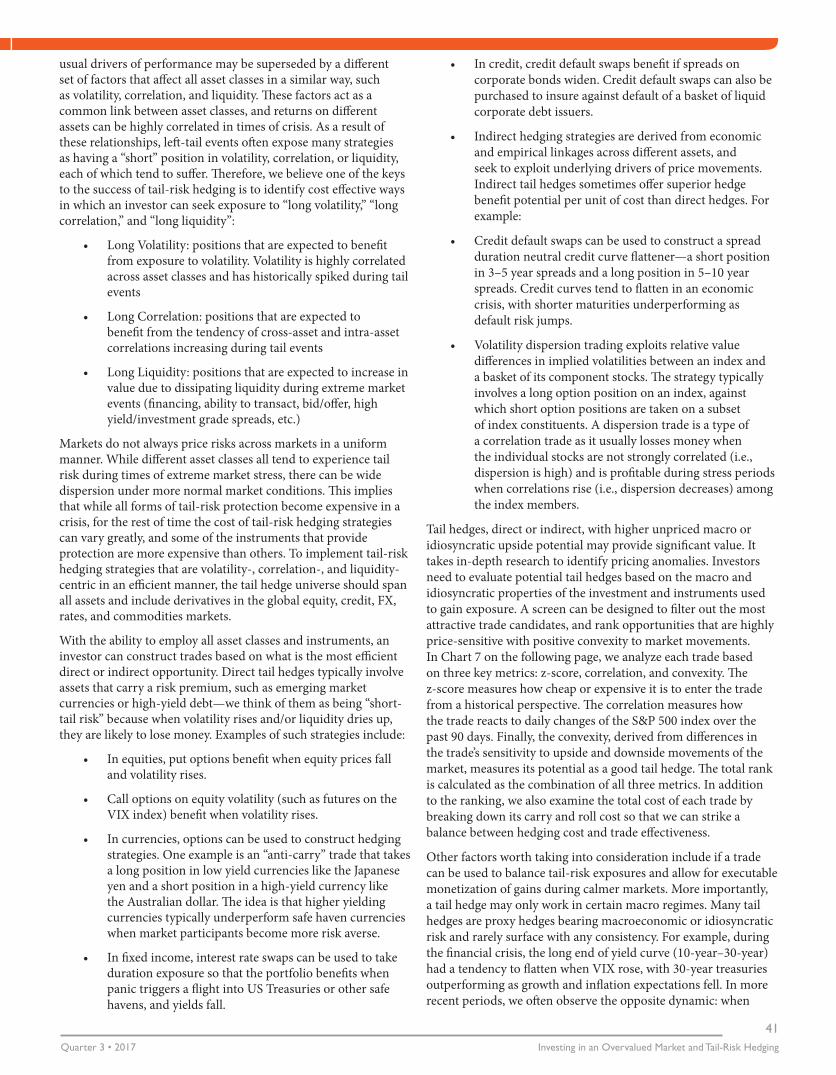
usual drivers of performance may be superseded by a different set of factors that affect all asset classes in a similar way, such as volatility, correlation, and liquidity. These factors act as a common link between asset classes, and returns on different assets can be highly correlated in times of crisis. As a result of these relationships, left-tail events often expose many strategies as having a “short” position in volatility, correlation, or liquidity, each of which tend to suffer. Therefore, we believe one of the keys to the success of tail-risk hedging is to identify cost effective ways in which an investor can seek exposure to “long volatility,” “long correlation,” and “long liquidity”:

• Long Volatility: positions that are expected to benefit from exposure to volatility. Volatility is highly correlated across asset classes and has historically spiked during tail events

• Long Correlation: positions that are expected to benefit from the tendency of cross-asset and intra-asset correlations increasing during tail events

• Long Liquidity: positions that are expected to increase in value due to dissipating liquidity during extreme market events (financing, ability to transact, bid/offer, high yield/investment grade spreads, etc.)

Markets do not always price risks across markets in a uniform manner. While different asset classes all tend to experience tail risk during times of extreme market stress, there can be wide dispersion under more normal market conditions. This implies that while all forms of tail-risk protection become expensive in a crisis, for the rest of time the cost of tail-risk hedging strategies can vary greatly, and some of the instruments that provide protection are more expensive than others. To implement tail-risk hedging strategies that are volatility-, correlation-, and liquidity-centric in an efficient manner, the tail hedge universe should span all assets and include derivatives in the global equity, credit, FX, rates, and commodities markets.

With the ability to employ all asset classes and instruments, an investor can construct trades based on what is the most efficient direct or indirect opportunity. Direct tail hedges typically involve assets that carry a risk premium, such as emerging market currencies or high-yield debt—we think of them as being “short-tail risk” because when volatility rises and/or liquidity dries up, they are likely to lose money. Examples of such strategies include:

• In equities, put options benefit when equity prices fall and volatility rises.

• Call options on equity volatility (such as futures on the VIX index) benefit when volatility rises.

• In currencies, options can be used to construct hedging strategies. One example is an “anti-carry” trade that takes a long position in low yield currencies like the Japanese yen and a short position in a high-yield currency like the Australian dollar. The idea is that higher yielding currencies typically underperform safe haven currencies when market participants become more risk averse.

• In fixed income, interest rate swaps can be used to take duration exposure so that the portfolio benefits when panic triggers a flight into US Treasuries or other safe havens, and yields fall.

• In credit, credit default swaps benefit if spreads on corporate bonds widen. Credit default swaps can also be purchased to insure against default of a basket of liquid corporate debt issuers.

• Indirect hedging strategies are derived from economic and empirical linkages across different assets, and seek to exploit underlying drivers of price movements. Indirect tail hedges sometimes offer superior hedge benefit potential per unit of cost than direct hedges. For example:

• Credit default swaps can be used to construct a spread duration neutral credit curve flattener—a short position in 3–5 year spreads and a long position in 5–10 year spreads. Credit curves tend to flatten in an economic crisis, with shorter maturities underperforming as default risk jumps.

• Volatility dispersion trading exploits relative value differences in implied volatilities between an index and a basket of its component stocks. The strategy typically involves a long option position on an index, against which short option positions are taken on a subset of index constituents. A dispersion trade is a type of a correlation trade as it usually losses money when the individual stocks are not strongly correlated (i.e., dispersion is high) and is profitable during stress periods when correlations rise (i.e., dispersion decreases) among the index members.

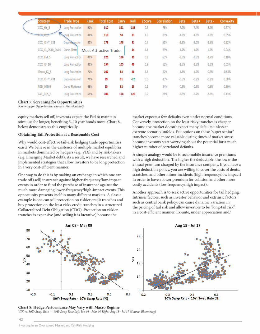
Tail hedges, direct or indirect, with higher unpriced macro or idiosyncratic upside potential may provide significant value. It takes in-depth research to identify pricing anomalies. Investors need to evaluate potential tail hedges based on the macro and idiosyncratic properties of the investment and instruments used to gain exposure. A screen can be designed to filter out the most attractive trade candidates, and rank opportunities that are highly price-sensitive with positive convexity to market movements. In Chart 7 on the following page, we analyze each trade based on three key metrics: z-score, correlation, and convexity. The z-score measures how cheap or expensive it is to enter the trade from a historical perspective. The correlation measures how the trade reacts to daily changes of the S&P 500 index over the past 90 days. Finally, the convexity, derived from differences in the trade’s sensitivity to upside and downside movements of the market, measures its potential as a good tail hedge. The total rank is calculated as the combination of all three metrics. In addition to the ranking, we also examine the total cost of each trade by breaking down its carry and roll cost so that we can strike a balance between hedging cost and trade effectiveness.

Other factors worth taking into consideration include if a trade can be used to balance tail-risk exposures and allow for executable monetization of gains during calmer markets. More importantly, a tail hedge may only work in certain macro regimes. Many tail hedges are proxy hedges bearing macroeconomic or idiosyncratic risk and rarely surface with any consistency. For example, during the financial crisis, the long end of yield curve (10-year–30-year) had a tendency to flatten when VIX rose, with 30-year treasuries outperforming as growth and inflation expectations fell. In more recent periods, we often observe the opposite dynamic: when

42Investing in an Overvalued Market and Tail-Risk Hedging

equity markets sell off, investors expect the Fed to maintain stimulus for longer, benefiting 5–10 year bonds more. Chart 8, below demonstrates this empirically.

Obtaining Tail Protection at a Reasonable Cost

Why would cost-effective tail-risk hedging trade opportunities exist? We believe in the existence of multiple market equilibria in markets dominated by hedgers (e.g. VIX) and by risk-takers (e.g. Emerging Market debt). As a result, we have researched and implemented strategies that allow investors to be long protection in a very cost-efficient manner.

One way to do this is by making an exchange in which one can trade off (sell) insurance against higher-frequency/low-impact events in order to fund the purchase of insurance against the much more damaging lower-frequency/high-impact events. This opportunity presents itself in many different markets. A classic example is one can sell protection on riskier credit tranches and buy protection on the least risky credit tranches in a structured Collateralized Debt Obligation (CDO). Protection on riskier tranches is expensive (and selling it is lucrative) because the

market expects a few defaults even under normal conditions. Conversely, protection on the least risky tranches is cheaper because the market doesn’t expect many defaults unless an extreme scenario unfolds. Put options on these “super senior” tranches become more valuable during times of market stress because investors start worrying about the potential for a much higher number of correlated defaults.

A simple analogy would be to automobile insurance premiums with a high deductible. The higher the deductible, the lower the annual premium charged by the insurance company. If you have a high deductible policy, you are willing to cover the costs of dents, scratches, and other minor incidents (high frequency/low impact) in order to have a lower premium for collision and other more costly accidents (low frequency/high impact).

Another approach is to seek active opportunities for tail hedging. Intrinsic factors, such as investor behavior and extrinsic factors, such as central bank policy, can cause dynamic variation in the pricing of tail risk and allow investors to be “long-tail risk” in a cost-efficient manner. Ex-ante, under appreciation and/

Chart 7: Screening for Opportunities Screening for Opportunities (Source: PhaseCapital)

Chart 8: Hedge Performance May Vary with Macro Regime VIX vs. 30Yr Swap Rate — 10Yr Swap Rate Left: Jan 08– Mar 09 Right: Aug 15– Jul 17 (Source: Bloomberg)

Investing in an Overvalued Market and Tail-Risk HedgingQuarter 3 • 2017

43

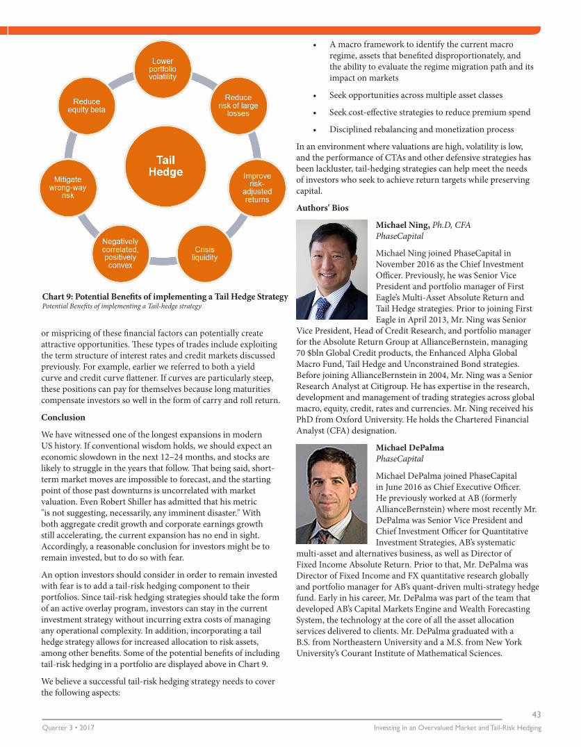
Chart 9: Potential Benefits of implementing a Tail Hedge Strategy Potential Benefits of implementing a Tail-hedge strategy

or mispricing of these financial factors can potentially create attractive opportunities. These types of trades include exploiting the term structure of interest rates and credit markets discussed previously. For example, earlier we referred to both a yield curve and credit curve flattener. If curves are particularly steep, these positions can pay for themselves because long maturities compensate investors so well in the form of carry and roll return.

Conclusion

We have witnessed one of the longest expansions in modern US history. If conventional wisdom holds, we should expect an economic slowdown in the next 12–24 months, and stocks are likely to struggle in the years that follow. That being said, short-term market moves are impossible to forecast, and the starting point of those past downturns is uncorrelated with market valuation. Even Robert Shiller has admitted that his metric "is not suggesting, necessarily, any imminent disaster." With both aggregate credit growth and corporate earnings growth still accelerating, the current expansion has no end in sight. Accordingly, a reasonable conclusion for investors might be to remain invested, but to do so with fear.

An option investors should consider in order to remain invested with fear is to add a tail-risk hedging component to their portfolios. Since tail-risk hedging strategies should take the form of an active overlay program, investors can stay in the current investment strategy without incurring extra costs of managing any operational complexity. In addition, incorporating a tail hedge strategy allows for increased allocation to risk assets, among other benefits. Some of the potential benefits of including tail-risk hedging in a portfolio are displayed above in Chart 9.

We believe a successful tail-risk hedging strategy needs to cover the following aspects:

• A macro framework to identify the current macro regime, assets that benefited disproportionately, and the ability to evaluate the regime migration path and its impact on markets

• Seek opportunities across multiple asset classes

• Seek cost-effective strategies to reduce premium spend

• Disciplined rebalancing and monetization process

In an environment where valuations are high, volatility is low, and the performance of CTAs and other defensive strategies has been lackluster, tail-hedging strategies can help meet the needs of investors who seek to achieve return targets while preserving capital.

Authors' Bios

Michael Ning, Ph.D, CFA PhaseCapital

Michael Ning joined PhaseCapital in November 2016 as the Chief Investment Officer. Previously, he was Senior Vice President and portfolio manager of First Eagle’s Multi-Asset Absolute Return and Tail Hedge strategies. Prior to joining First Eagle in April 2013, Mr. Ning was Senior

Vice President, Head of Credit Research, and portfolio manager for the Absolute Return Group at AllianceBernstein, managing 70 $bln Global Credit products, the Enhanced Alpha Global Macro Fund, Tail Hedge and Unconstrained Bond strategies. Before joining AllianceBernstein in 2004, Mr. Ning was a Senior Research Analyst at Citigroup. He has expertise in the research, development and management of trading strategies across global macro, equity, credit, rates and currencies. Mr. Ning received his PhD from Oxford University. He holds the Chartered Financial Analyst (CFA) designation.

Michael DePalma PhaseCapital

Michael DePalma joined PhaseCapital in June 2016 as Chief Executive Officer. He previously worked at AB (formerly AllianceBernstein) where most recently Mr. DePalma was Senior Vice President and Chief Investment Officer for Quantitative Investment Strategies, AB’s systematic

multi-asset and alternatives business, as well as Director of Fixed Income Absolute Return. Prior to that, Mr. DePalma was Director of Fixed Income and FX quantitative research globally and portfolio manager for AB’s quant-driven multi-strategy hedge fund. Early in his career, Mr. DePalma was part of the team that developed AB’s Capital Markets Engine and Wealth Forecasting System, the technology at the core of all the asset allocation services delivered to clients. Mr. DePalma graduated with a B.S. from Northeastern University and a M.S. from New York University’s Courant Institute of Mathematical Sciences.