Seminar on Regionalism and the WTO, Geneva, 14 November 2003

The Case for Free Trade and the Role of RTAs

by

P. J. Lloyd and

Donald MacLaren

University of Melbourne

Address for Correspondence: Department of Economics, Faculty of Economics and commerce, The University of Melbourne, Parkville, Victoria 3010, Australia Phone: 61 3 83445291

61 3 83445035 Fax 61 3 83446899 Email: pjlloyd@unimelb.edu.au d.maclaren@unimelb.edu.au

The Case for Free Trade and the Role of RTAs

With the extraordinary and unprecedented level of activity post-Cancun regarding

negotiations and explorations of future RTAs, it is imperative that trade economists have a

clear view of the basic economics of RTAs. This paper sets out the main themes from the

theory of discriminatory trading areas. It is concerned solely with trade in goods. Despite

the introduction into the WTO agenda of trade in services and the Singapore issues and

beyond the border regulations more generally, goods trade discrimination remains the central

issue in the debate about RTAs.

1. The predictions of trade theory

The way economic theorists have viewed discriminatory trade blocs has changed over time.

At the time of the formation of the GATT in 1948, RTAs were viewed as a step towards free

global trade. Provided new RTAs did not raise trade barriers vis-à-vis the Rest of the World,

they resulted in an overall lowering of trade barriers in the world economy and this was

regarded as benign. Article XXIV is based on this view.

Viner (1950) changed this perception dramatically. Viner recognised that the trade induced

by a free trade area or a customs union was of two types, which he called trade creation and

trade diversion. The former is the substitution of a lower cost source of supply within the

area for a more costly source in the importing country and is, therefore, beneficial to the

member countries and the world as a whole. By contrast, trade diversion is the substitution

of a more costly source of supply within the area for a less costly source outside the area.

This led Viner to his famous prediction:

“…where the trade-diverting effect is predominant, one at least of the member

countries is bound to be injured, the two combined will suffer a net injury, and there

will be injury to the outside world and to the world at large.” (Viner, 1950, p. 44)

Within a few years of the publication of Viner’s book, a number of writers demonstrated that

some part or parts of Viner’s predictions may not hold. In particular, a number of papers

provided examples where the country to which trade is diverted, the importing country, may

gain when trade diversion occurs. The key publications were those of Meade (1955),

Gehrels (1956-57), Lipsey (1957) and Michaely (1965).

2

Because of the limited technology of handling general equilibrium models at that time, most

of these authors used models of a single country. All of these early models were also very

limited in dimensionality to models with three countries and only two or three goods and the

structure of the economies was simplified; for example, all production processes were fully

integrated with no international trade in intermediate inputs. We need to generalise the

results to models of higher dimensionality and more general structure.1

There are today a variety of models that can be used to analyse the effects of an RTA.

Following Baldwin and Venables (1995), general equilibrium models with trade can be

grouped into three generations. The first is the traditional trade model that assumes constant

returns to scale, perfect competition and a fixed number of goods. The second is the

generation of models known as New Trade Theory that emerged in the 1980s. This theory

has increasing returns to scale in some industries at least, imperfect competition and the

number of the varieties of goods is endogenous. The third is the later generation of models

that introduced investment and growth effects. The first-generation models are still relevant

because they cover most of the theory of trade discrimination and most computable general

equilibrium models are in this tradition.

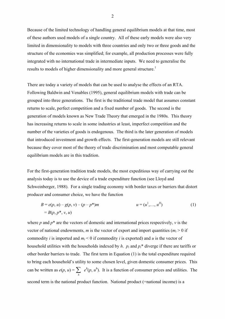
For the first-generation tradition trade models, the most expeditious way of carrying out the

analysis today is to use the device of a trade expenditure function (see Lloyd and

Schweinberger, 1988). For a single trading economy with border taxes or barriers that distort

producer and consumer choice, we have the function

B = e(p, u) – g(p, v) – (p – p*)m u = (u1,…, uH) (1)

= B(p, p*, v, u)

where p and p* are the vectors of domestic and international prices respectively, v is the

vector of national endowments, m is the vector of export and import quantities (mi > 0 if

commodity i is imported and mi < 0 if commodity i is exported) and u is the vector of

household utilities with the households indexed by h. pi and pi* diverge if there are tariffs or

other border barriers to trade. The first term in Equation (1) is the total expenditure required

to bring each household’s utility to some chosen level, given domestic consumer prices. This

can be written as e(p, u) = ∑ eh

h(p, uh). It is a function of consumer prices and utilities. The

second term is the national product function. National product (=national income) is a

3

function of the domestic producer prices and endowments. The third term is the aggregate

trade tax revenue. B is then the compensation needed to allow the households to reach the

chosen levels of utility, after the households have received income from national production

and the net trade tax revenue has been distributed lump sum to them. In the absence of any

transfer from outside the economy, B = 0.

This function applies to an economy with a very general Neoclassical structure. There are no

restrictions on the numbers of final goods, factors or households and the structure of

production permits traded intermediate inputs and specific and non-specific inputs. This

approach does not require a single household or the artifice that there exists a social utility

function that represents the preferences of the households. It is general equilibrium analysis

as both the national product function and the national expenditure functions are derived from

optimising behaviour over all agents, mutatis mutandis. The model does, however, rule out

economies of scale and non-competitive behaviour.

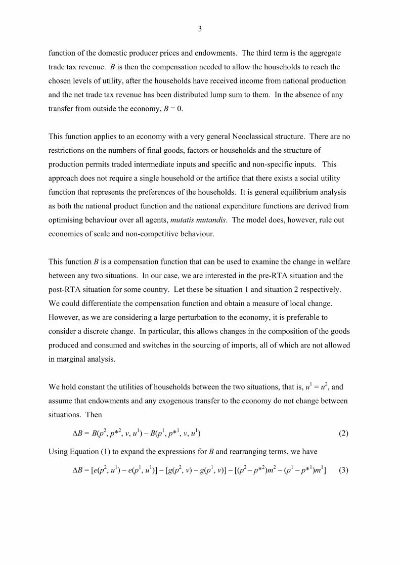
This function B is a compensation function that can be used to examine the change in welfare

between any two situations. In our case, we are interested in the pre-RTA situation and the

post-RTA situation for some country. Let these be situation 1 and situation 2 respectively.

We could differentiate the compensation function and obtain a measure of local change.

However, as we are considering a large perturbation to the economy, it is preferable to

consider a discrete change. In particular, this allows changes in the composition of the goods

produced and consumed and switches in the sourcing of imports, all of which are not allowed

in marginal analysis.

We hold constant the utilities of households between the two situations, that is, u1 = u2, and

assume that endowments and any exogenous transfer to the economy do not change between

situations. Then

∆B = B(p2, p*2, v, u1) – B(p1, p*1, v, u1) (2)

Using Equation (1) to expand the expressions for B and rearranging terms, we have

∆B = [e(p2, u1) – e(p1, u1)] – [g(p2, v) – g(p1, v)] – [(p2 – p*2)m2 – (p1 – p*1)m1] (3)

4

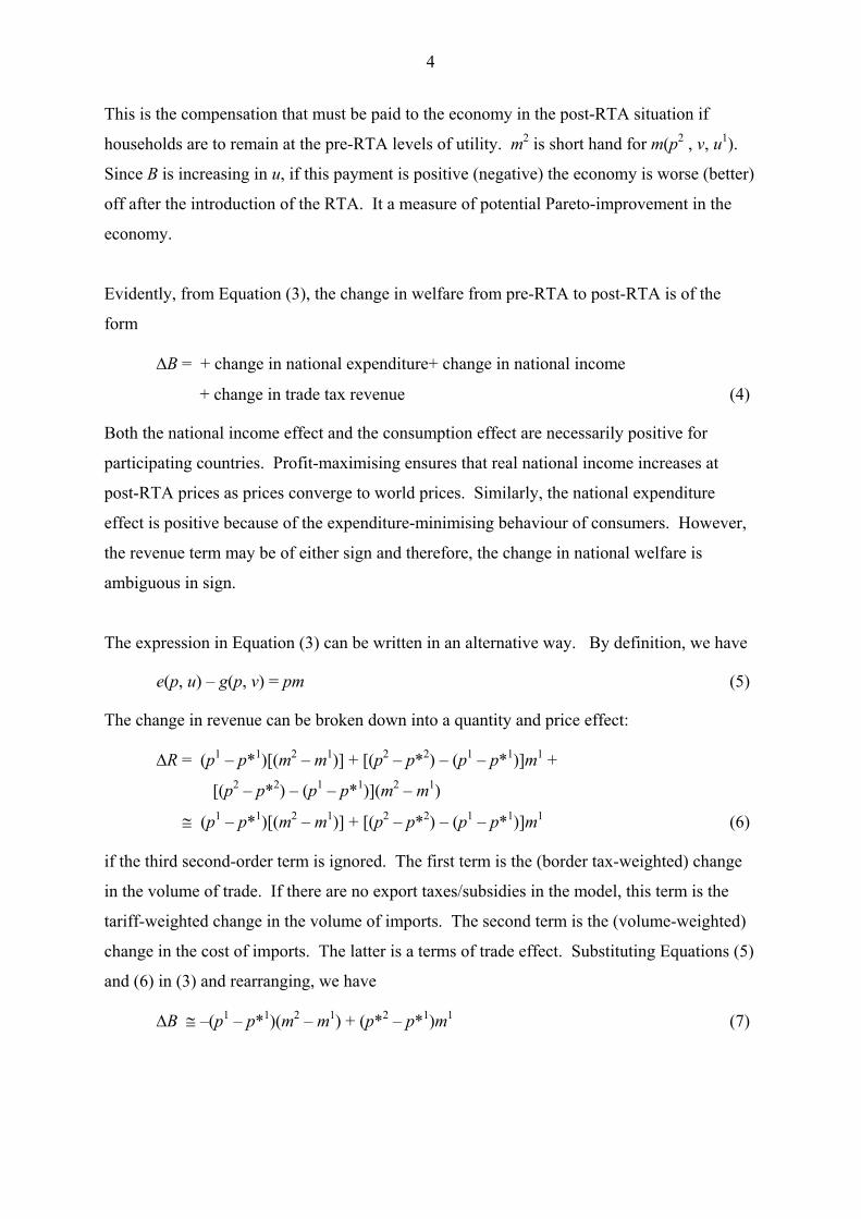
This is the compensation that must be paid to the economy in the post-RTA situation if

households are to remain at the pre-RTA levels of utility. m2 is short hand for m(p2 , v, u1).

Since B is increasing in u, if this payment is positive (negative) the economy is worse (better)

off after the introduction of the RTA. It a measure of potential Pareto-improvement in the

economy.

Evidently, from Equation (3), the change in welfare from pre-RTA to post-RTA is of the

form

∆B = + change in national expenditure+ change in national income

+ change in trade tax revenue (4)

Both the national income effect and the consumption effect are necessarily positive for

participating countries. Profit-maximising ensures that real national income increases at

post-RTA prices as prices converge to world prices. Similarly, the national expenditure

effect is positive because of the expenditure-minimising behaviour of consumers. However,

the revenue term may be of either sign and therefore, the change in national welfare is

ambiguous in sign.

The expression in Equation (3) can be written in an alternative way. By definition, we have

e(p, u) – g(p, v) = pm (5)

The change in revenue can be broken down into a quantity and price effect:

∆R = (p1 – p*1)[(m2 – m1)] + [(p2 – p*2) – (p1 – p*1)]m1 +

[(p2 – p*2) – (p1 – p*1)](m2 – m1)

≅ (p1 – p*1)[(m2 – m1)] + [(p2 – p*2) – (p1 – p*1)]m1 (6)

if the third second-order term is ignored. The first term is the (border tax-weighted) change

in the volume of trade. If there are no export taxes/subsidies in the model, this term is the

tariff-weighted change in the volume of imports. The second term is the (volume-weighted)

change in the cost of imports. The latter is a terms of trade effect. Substituting Equations (5)

and (6) in (3) and rearranging, we have

∆B ≅ –(p1 – p*1)(m2 – m1) + (p*2 – p*1)m1 (7)

5

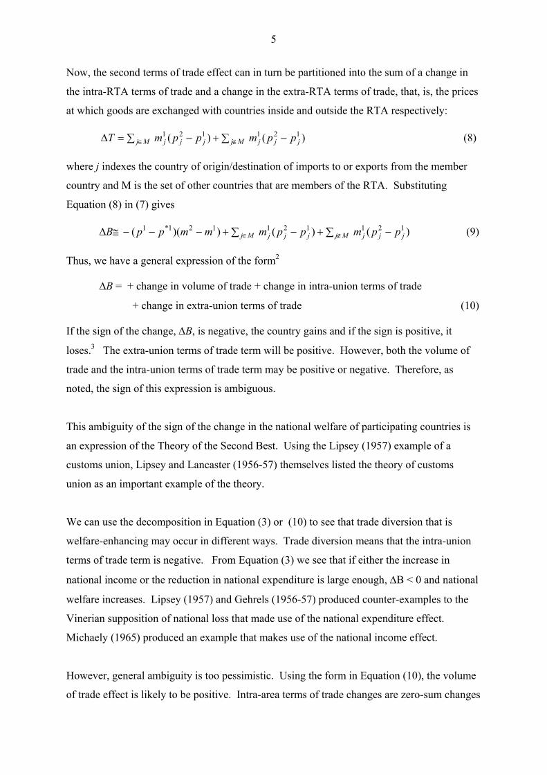
Now, the second terms of trade effect can in turn be partitioned into the sum of a change in

the intra-RTA terms of trade and a change in the extra-RTA terms of trade, that, is, the prices

at which goods are exchanged with countries inside and outside the RTA respectively:

(8) ∑ −+−∑=∆ ∉∈ Mj jjjjjMj j ppmppmT )()( 121121

where j indexes the country of origin/destination of imports to or exports from the member

country and M is the set of other countries that are members of the RTA. Substituting

Equation (8) in (7) gives

∆B≅ (9) ∑ −+−∑+−−− ∉∈ Mj jjjjjMj j ppmppmmmpp )()())(( 121121121*1

Thus, we have a general expression of the form2

∆B = + change in volume of trade + change in intra-union terms of trade

+ change in extra-union terms of trade (10)

If the sign of the change, ∆B, is negative, the country gains and if the sign is positive, it

loses.3 The extra-union terms of trade term will be positive. However, both the volume of

trade and the intra-union terms of trade term may be positive or negative. Therefore, as

noted, the sign of this expression is ambiguous.

This ambiguity of the sign of the change in the national welfare of participating countries is

an expression of the Theory of the Second Best. Using the Lipsey (1957) example of a

customs union, Lipsey and Lancaster (1956-57) themselves listed the theory of customs

union as an important example of the theory.

We can use the decomposition in Equation (3) or (10) to see that trade diversion that is

welfare-enhancing may occur in different ways. Trade diversion means that the intra-union

terms of trade term is negative. From Equation (3) we see that if either the increase in

national income or the reduction in national expenditure is large enough, ∆B < 0 and national

welfare increases. Lipsey (1957) and Gehrels (1956-57) produced counter-examples to the

Vinerian supposition of national loss that made use of the national expenditure effect.

Michaely (1965) produced an example that makes use of the national income effect.

However, general ambiguity is too pessimistic. Using the form in Equation (10), the volume

of trade effect is likely to be positive. Intra-area terms of trade changes are zero-sum changes

6

for the area as whole as one member country’s gain is another’s loss. The extra-union effect

will be positive for at least one member (see below). Thus, there is a presumption that

participating countries gain. A loss requires large negative revenue effects due to an adverse

movement of the terms of trade or, less likely, a reduced volume of trade.

This presumption overturns Viner with respect to the welfare of the participating countries.

Yet, many trade economists as well as non-trade economists continue to couch the outcome

of actual or prospective RTAs in terms of whether the volume of trade created dominates the

volume of trade diverted; for example, recently a number of authors have used gravity

models with the volume of trade as the dependent variable to test the effects of the formation

of RTAs. These authors seem not to have understood the post-Viner literature. They use a

criterion of national gain/loss in terms of the effect of an RTA on the volume when they

should use some criterion of national welfare.

With respect to the welfare of non-participating countries, the outcome is quite different. The

shock of the formation of an RTA registers for non-participating countries via a change in the

terms at which they trade. They gain or lose from the formation of an RTA depending on

whether their terms of trade improve or deteriorate. Trade diversion necessarily worsens the

terms of trade of an outside country whose trade has been diverted but this is not the end of it.

Income effects and other indirect price effects from the RTA may increase demand for

outside countries’ exports or increase supplies of the goods they import relative to the initial

pre-RTA equilibrium. One requires a general equilibrium analysis to determine the final

changes in the terms of trade of third countries, and of course the participating countries too.

A small number of authors has analysed the effects of the formation of an RTA on terms of

trade in models in which there are three countries and three commodities, the 3x3 models.

The Meade (1955) model is a symmetric model with three goods and three countries. Each

country produces and exports one good and imports two goods. Because of this symmetry,

each good is imported from only one country, the only country that produces that good. The

other model is that of Riezman (1979). This too is symmetric in its basic production-

consumption structure. In this model, each country produces and imports only one good and

exports two. Because of this symmetry, each good is exported by two countries.

Consequently there is a prospect of trade diversion in both member countries in the Riezman

model, but there can be no trade diversion in either member country in the Meade model.

7

In the Meade model, the terms of trade of at least one of the two member countries must

improve and there is a presumption, under regularity conditions, that the terms of trade of

both may improve. In all cases, Mundell (1964) proved that the terms of trade of the outside

country must deteriorate. However, Mundell’s analysis takes no account of the income

effects in member countries. These effects may offset the negative price effects so that the

terms of trade of the third country may improve.

The Riezman model is the more interesting in this context. It is a general equilibrium model

of the world economy with endogenous terms of trade. Riezman divides the effects on the

terms of trade of the participating countries into the two components, the intra-area and extra-

area terms of trade. He finds that the sign of the change in the intra-union terms of trade is

ambiguous but, for both countries, the extra-union terms of trade must increase.

Consequently, the outside country must lose.

These results conform to Viner’s prediction with respect to the outside country.4 In models

with more than one outside country, the terms of trade of an outside country may improve

though one can still expect that the terms of trade of outside countries collectively will

deteriorate. The welfare of outside countries should be the major concern of policy analysts.

Kemp and Wan (1976) introduced an important line of thought that changed perceptions of

RTAs. They proved that a customs union that adjusts its common external tariff so as to

leave the volume of trade with outside countries unchanged and introduces a system of lump-

sum payments among members only will make households in both member and non-member

countries better off or at the least no worse off. The gain to member countries stems from the

positive national income and national expenditure effects of the removal of distortions within

the union, given fixed trade with outside countries. The existence of a common external

tariff which preserves trade with outside countries at the pre-RTA levels removes any harm

to these countries. Given the results for outside countries above, we can expect that the RTA

will worsen the terms of trade of outside countries and, therefore, the adjustment will be to

lower the common external tariff rates. This demonstrated a universal possibility of gain to

outside countries and the world as whole.

8

Subsequently, Grinols (1981) showed how the compensation scheme could be implemented

as a function of its pre-union trade vector and Srinivasan (1997) showed how the common

external tariff could be implemented as an average of the pre-union tariff rates of the member

countries. Ohyama (2002) and Panagariya and Krishna (2002) independently extended this

theorem to the numerically more important case of free trade areas that do not have common

external tariff rates. In the case of free trade areas, each member country must adjust its tariff

rates so as to keep the volume of its trade with outside countries unchanged.

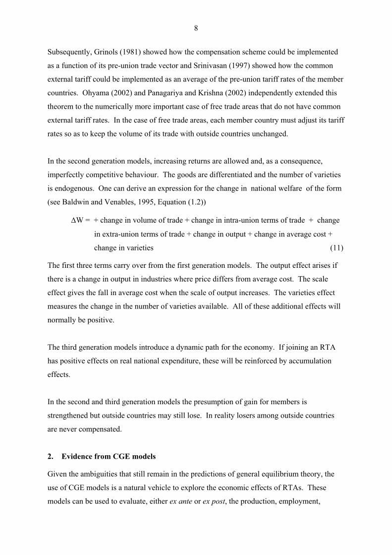
In the second generation models, increasing returns are allowed and, as a consequence,

imperfectly competitive behaviour. The goods are differentiated and the number of varieties

is endogenous. One can derive an expression for the change in national welfare of the form

(see Baldwin and Venables, 1995, Equation (1.2))

∆W = + change in volume of trade + change in intra-union terms of trade + change

in extra-union terms of trade + change in output + change in average cost +

change in varieties (11)

The first three terms carry over from the first generation models. The output effect arises if

there is a change in output in industries where price differs from average cost. The scale

effect gives the fall in average cost when the scale of output increases. The varieties effect

measures the change in the number of varieties available. All of these additional effects will

normally be positive.

The third generation models introduce a dynamic path for the economy. If joining an RTA

has positive effects on real national expenditure, these will be reinforced by accumulation

effects.

In the second and third generation models the presumption of gain for members is

strengthened but outside countries may still lose. In reality losers among outside countries

are never compensated.

2. Evidence from CGE models

Given the ambiguities that still remain in the predictions of general equilibrium theory, the

use of CGE models is a natural vehicle to explore the economic effects of RTAs. These

models can be used to evaluate, either ex ante or ex post, the production, employment,

9

consumption and trade effects, and the price and welfare effects of the formation or the

expansion of an RTA. In particular, a CGE model with suitably disaggregated

commodities/sectors and countries/regions is well-suited to running policy simulation

experiments on the formation of the common configurations of RTAs, namely, bilaterals,

plurilaterals and hub and spokes (see section 3 below).

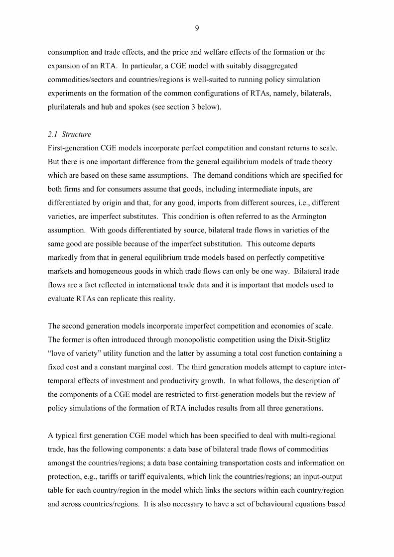
2.1 Structure

First-generation CGE models incorporate perfect competition and constant returns to scale.

But there is one important difference from the general equilibrium models of trade theory

which are based on these same assumptions. The demand conditions which are specified for

both firms and for consumers assume that goods, including intermediate inputs, are

differentiated by origin and that, for any good, imports from different sources, i.e., different

varieties, are imperfect substitutes. This condition is often referred to as the Armington

assumption. With goods differentiated by source, bilateral trade flows in varieties of the

same good are possible because of the imperfect substitution. This outcome departs

markedly from that in general equilibrium trade models based on perfectly competitive

markets and homogeneous goods in which trade flows can only be one way. Bilateral trade

flows are a fact reflected in international trade data and it is important that models used to

evaluate RTAs can replicate this reality.

The second generation models incorporate imperfect competition and economies of scale.

The former is often introduced through monopolistic competition using the Dixit-Stiglitz

“love of variety” utility function and the latter by assuming a total cost function containing a

fixed cost and a constant marginal cost. The third generation models attempt to capture inter-

temporal effects of investment and productivity growth. In what follows, the description of

the components of a CGE model are restricted to first-generation models but the review of

policy simulations of the formation of RTA includes results from all three generations.

A typical first generation CGE model which has been specified to deal with multi-regional

trade, has the following components: a data base of bilateral trade flows of commodities

amongst the countries/regions; a data base containing transportation costs and information on

protection, e.g., tariffs or tariff equivalents, which link the countries/regions; an input-output

table for each country/region in the model which links the sectors within each country/region

and across countries/regions. It is also necessary to have a set of behavioural equations based

10

on the economic theory of the assumed behaviour of individual firms and consumers.

Finally, there is a set of accounting identities. These identities track: the flows of household

expenditures to private consumption, to government, to imports and to savings; the flows of

income going to the household from wages, rents, and taxes raised on domestic transactions

and on traded goods and inputs; the flow of income to firms from selling goods and services

to consumers, to government, to other domestic firms and to exports; and the flow of

expenditures made by firms to the household, as providers of primary factors, to domestic

firms, as suppliers of intermediate inputs, and to imports.5

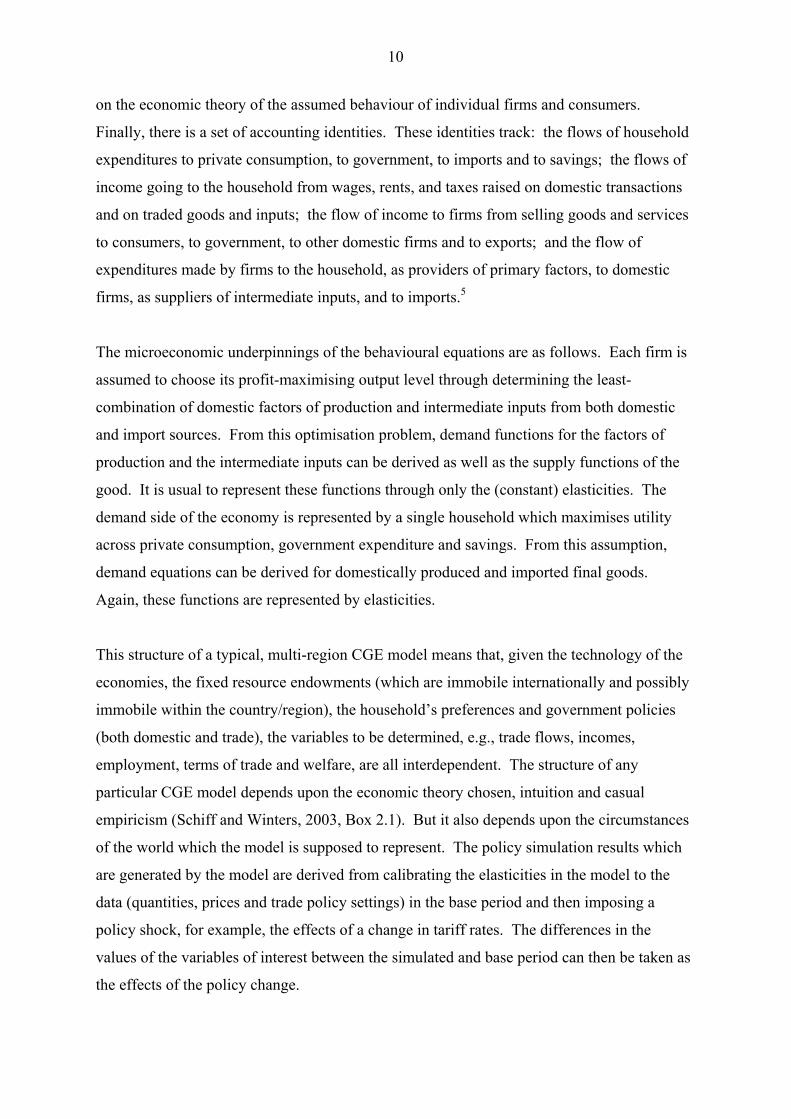
The microeconomic underpinnings of the behavioural equations are as follows. Each firm is

assumed to choose its profit-maximising output level through determining the least-

combination of domestic factors of production and intermediate inputs from both domestic

and import sources. From this optimisation problem, demand functions for the factors of

production and the intermediate inputs can be derived as well as the supply functions of the

good. It is usual to represent these functions through only the (constant) elasticities. The

demand side of the economy is represented by a single household which maximises utility

across private consumption, government expenditure and savings. From this assumption,

demand equations can be derived for domestically produced and imported final goods.

Again, these functions are represented by elasticities.

This structure of a typical, multi-region CGE model means that, given the technology of the

economies, the fixed resource endowments (which are immobile internationally and possibly

immobile within the country/region), the household’s preferences and government policies

(both domestic and trade), the variables to be determined, e.g., trade flows, incomes,

employment, terms of trade and welfare, are all interdependent. The structure of any

particular CGE model depends upon the economic theory chosen, intuition and casual

empiricism (Schiff and Winters, 2003, Box 2.1). But it also depends upon the circumstances

of the world which the model is supposed to represent. The policy simulation results which

are generated by the model are derived from calibrating the elasticities in the model to the

data (quantities, prices and trade policy settings) in the base period and then imposing a

policy shock, for example, the effects of a change in tariff rates. The differences in the

values of the variables of interest between the simulated and base period can then be taken as

the effects of the policy change.

11

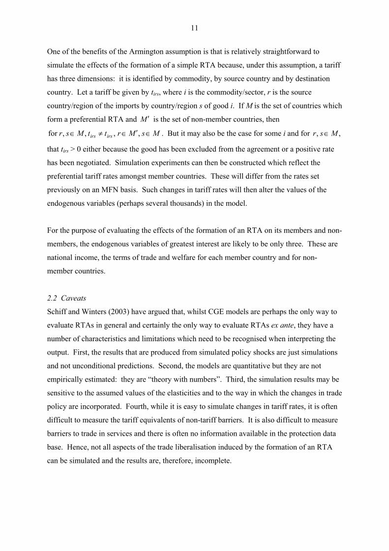
One of the benefits of the Armington assumption is that is relatively straightforward to

simulate the effects of the formation of a simple RTA because, under this assumption, a tariff

has three dimensions: it is identified by commodity, by source country and by destination

country. Let a tariff be given by tirs, where i is the commodity/sector, r is the source

country/region of the imports by country/region s of good i. If M is the set of countries which

form a preferential RTA and M ′

s∈,

is the set of non-member countries, then

. But it may also be the case for some i and for MMrttMsr irsirs ′∈≠∈ , , ,for ,, Msr ∈

that tirs > 0 either because the good has been excluded from the agreement or a positive rate

has been negotiated. Simulation experiments can then be constructed which reflect the

preferential tariff rates amongst member countries. These will differ from the rates set

previously on an MFN basis. Such changes in tariff rates will then alter the values of the

endogenous variables (perhaps several thousands) in the model.

For the purpose of evaluating the effects of the formation of an RTA on its members and non-

members, the endogenous variables of greatest interest are likely to be only three. These are

national income, the terms of trade and welfare for each member country and for non-

member countries.

2.2 Caveats

Schiff and Winters (2003) have argued that, whilst CGE models are perhaps the only way to

evaluate RTAs in general and certainly the only way to evaluate RTAs ex ante, they have a

number of characteristics and limitations which need to be recognised when interpreting the

output. First, the results that are produced from simulated policy shocks are just simulations

and not unconditional predictions. Second, the models are quantitative but they are not

empirically estimated: they are “theory with numbers”. Third, the simulation results may be

sensitive to the assumed values of the elasticities and to the way in which the changes in trade

policy are incorporated. Fourth, while it is easy to simulate changes in tariff rates, it is often

difficult to measure the tariff equivalents of non-tariff barriers. It is also difficult to measure

barriers to trade in services and there is often no information available in the protection data

base. Hence, not all aspects of the trade liberalisation induced by the formation of an RTA

can be simulated and the results are, therefore, incomplete.

12

A fifth important caveat concerns the Armington assumption. It is a useful, if ad hoc, way of

allowing for cross-hauling (intra-industry trade) in the trade flow data and it reduces the

number of parameters in the model. However, a combination of the Armington assumption

together with constant elasticity of substitution (CES) functions introduces a bias when these

appear in CGE models that are used to evaluate the effects of the formation of an RTA. The

bias arises because no matter how high the price of an import from a given source rises, the

quantity imported, while approaching zero, never reaches it. By contrast, in a simple partial

equilibrium model of an RTA, imports from the non-member country will become zero if its

tariff-inclusive price exceeds that of the member country’s price. In the CGE model, for each

good, i, imports from all sources, r, are each essential when combined in the CES functions

of firms and of consumers.6 The consequence is that there is a bias against finding trade

diversion and so the possible welfare losses for the non-member countries are understated. A

second consequence of the Armington assumption together with CES functions is that the

terms of trade effects of a change in trade policy can be implausibly large. The implication is

that the welfare gains from improvements in the terms of trade and welfare losses from a

deterioration in the terms of trade are exaggerated.7 Taking these partially offsetting effects

together, it is uncertain what the sign of the net bias may be for non-member countries.

2.3 Summary of Results

The summary that follows is, of necessity, highly selective but it is indicative of the results

obtained in the substantial literature. The regions to be reviewed are NAFTA, the EU and

APEC. To gain a sense of whether or not the formation of an RTA necessarily benefits the

region’s trading partners, it is instructive to consider the results of simulations on the

formation of NAFTA, the EU’s single market and a selection of RTAs which are being

discussed amongst several subsets of countries in APEC.

Brown et al. (1992) ran a number of simulations to represent the formation of NAFTA using

different assumptions about what was liberalised. Their model was a generation two CGE

model with four regions in each of which imperfect competition occurred in some sectors and

perfect competition occurred in others. When the authors assumed free trade in goods

amongst Canada, Mexico and the United States, the welfare gains (measured as a percentage

of pre-NAFTA GDP) were 0.7 per cent, 1.6 per cent and 0.1 per cent, respectively. They also

found that the welfare change for 31 excluded, other countries (industrialised and newly

industrialising) was −0.0. In all cases, the changes in welfare were small, showing gains to

13

the individual members of NAFTA and a loss to the aggregate group of 31 excluded

countries. When investment was also freed up (a generation three simulation), the gains to

the members of NAFTA became 0.7, 5.0 and 0.3, respectively. The additional gains to

Mexico are substantial and illustrate the points made above that the results are very sensitive

to the assumptions made in the policy simulation experiment, and that there are additional

gains from allowing for factor accumulation. The loss of welfare to the aggregate of

excluded countries remained at −0.0.

Haaland and Norman (1992) used a generation two CGE model to investigate the effects of

the EU single market. They restricted their experiment to a reduction of 2.5 percent on intra-

EU trade costs in manufactures from the formation of the single market; reductions in the

costs in services trade and changes in the integration of financial markets were excluded. An

additional assumption that they simulated was whether intra-EU markets remained

segmented or became integrated. They found a 0.40 per cent increase in EU welfare

(measured as the percentage change in GDP) when market segmentation persisted but a 0.64

per cent increase when the market was integrated. EFTA, as one of the EU’s trading

partners, experienced a 0.15 per cent decrease in the welfare in the segmented case and a 0.22

per cent decrease in the integrated case. This result is significant because it reveals the size

of the negative externality created by the deeper integration of the EU on one of its trading

partners, the size of the loss increasing as the degree of intra-EU market integration increases.

One of the early sets of results on the proposed ‘open regionalism’ of APEC was by Young

and Huff (1997). In a 10-region, 3-commodity aggregation of the GTAP model using version

2 of the data base, they compared outcomes for three experiments of trade liberalisation. In

experiment 1, it was assumed that all tariff and non-tariff barriers were removed amongst

APEC members but there was no change against the rest of the world (ROW). They found

that some members gained in terms of welfare, others lost and ROW lost. The losses ranged

from −0.17 per cent of base period household utility to −3.05 per cent, while the gains ranged

from 1.28 per cent to 3.16 per cent. When non-reciprocal APEC liberalisation occurred with

ROW, the pattern of gainers and losers amongst members was broadly similar to that in

experiment 1 but ROW now gained (0.19 per cent of base period household utility). In

experiment 3, it was assumed that ROW reciprocated the APEC region’s trade liberalisation.

The pattern of gainers and losers amongst members of APEC changed and ROW lost relative

14

to the base and by even more than it did in experiment 1, namely, by −0.51 per cent as

compared with −0.34 per cent.

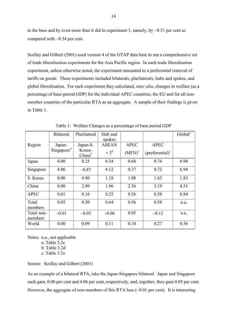
Scollay and Gilbert (2001) used version 4 of the GTAP data base to run a comprehensive set

of trade liberalisation experiments for the Asia Pacific region. In each trade liberalisation

experiment, unless otherwise noted, the experiment amounted to a preferential removal of

tariffs on goods. These experiments included bilaterals, plurilaterals, hubs and spokes, and

global liberalisation. For each experiment they calculated, inter alia, changes in welfare (as a

percentage of base-period GDP) for the individual APEC countries, the EU and for all non-

member countries of the particular RTA as an aggregate. A sample of their findings is given

in Table 1.

Table 1: Welfare Changes as a percentage of base period GDP

Bilateral Plurilateral Hub and spokes

Globalc

Region Japan-Singaporea

Japan-S. Korea-Chinab

ASEAN

+ 3b

APEC

(MFN)c

APEC

(preferential)c

Japan 0.00 0.25 0.34 0.68 0.74 0.98

Singapore 4.06 −0.87 4.12 0.37 0.72 6.94

S. Korea 0.00 0.80 1.18 1.08 1.63 1.83

China 0.00 2.09 1.96 2.56 3.19 4.51

APEC 0.01 0.16 0.25 0.56 0.58 0.84

Total members

0.05 0.50 0.64 0.56 0.58 n.a.

Total non-members

−0.01 −0.03 −0.06 0.05 −0.12 n.a.

World 0.00 0.09 0.11 0.34 0.27 0.56

Notes: n.a., not applicable a: Table 3.2c b: Table 3.2d c: Table 3.2e Source: Scollay and Gilbert (2001)

As an example of a bilateral RTA, take the Japan-Singapore bilateral. Japan and Singapore

each gain, 0.00 per cent and 4.06 per cent, respectively, and, together, they gain 0.05 per cent.

However, the aggregate of non-members of this RTA lose (−0.01 per cent). It is interesting

15

to compare these results with those from a different version of the GTAP model and a

different data base. Hertel et al. used a dynamic version of the GTAP model (a generation

three model) and included in their experiment what they referred to ‘new age’ elements in

this RTA, for example, rules covering FDI, e-commerce, trade in services and customs

procedures. By running a series of experiments, beginning with tariff liberalisation for trade

in goods only, and then adding successively each of these new age elements, they obtained

the following results for the year 2020. Japan would lose from tariff-only liberalisation (~

−0.0019 per cent) but would gain 0.157 per cent when all the features of the RTA are

accounted for. The corresponding figures for Singapore were ~ 0.09 per cent and 0.668 per

cent, respectively. Non-member countries individually lose in the tariff-only simulation but

gain from the full RTA.

As an example of a plurilateral RTA, take the Japan-South Korea-China plurilateral. Japan,

South Korea and China all gain, 0.25 per cent, 0.80 per cent and 2.09 per cent (Table 1).

Most APEC countries in South East Asia lose, e.g., Singapore (−0.87 per cent). The

members of the RTA gain 0.50 per cent while the aggregate of non-member countries lose

(−0.03 per cent). As an example of a hub and spokes arrangement, consider the example of

ASEAN+3. The ‘3’ gain individually (Japan by 0.34 per cent, South Korea by 1.18 per cent

and China by 1.96 per cent) and collectively (0.64 per cent), while the aggregate of non-

members lose (−0.06 per cent). Using the Michigan model of world trade (a generation two

CGE model) with version 4 of the GTAP data base, Brown et al. (2003) also simulated the

ASEAN+3 RTA but using 2005 as the base year, the year in which all post Uruguay Round

liberalisations are to be fully implemented. They found that if all members were to eliminate

all tariffs on agricultural products and manufactures, and remove barriers to services, then

there would be the following welfare gains. Japan would gain 2.62 per cent of base period

GDP, Singapore 10.66 per cent, South Korea 4.21 per cent and China 1.95 per cent. The

magnitudes of these numbers, and the ranking of these countries by the size of the gains, are

quite different from those of Scollay and Gilbert.

If APEC countries were to liberalise on an MFN basis, then most, but not all, of the member

countries would gain, the aggregate for the group being 0.56 per cent (Table 1). Moreover,

the aggregate of non-member countries would also gain (0.05 per cent). However, if APEC

were to liberalise on a preferential basis, then again, most but not all members would gain,

16

with the APEC countries as a group gaining 0.58 per cent. The aggregate of the non-APEC

countries would now lose (−0.12). Brown et al. (2003) found that, for a similar experiment,

the gain to Japan was 4.9 per cent (c.f. Scollay and Gilbert’s value of 0.74 per cent). Finally,

multilateral, global liberalisation leads to the largest gains for each of the countries and RTA

groupings identified in Table 1, as well as for the world economy. This is also a conclusion

from the simulations conducted by Brown et al. (2003).

A number of overall conclusions can be drawn from these results. First, global multilateral

trade liberalisation generates the greatest gains to the world economy (0.56 per cent).

Second, if the members of APEC liberalise on an MFN basis (“open regionalism”) rather

than on a preferential basis, then the gains to the world economy are greater (0.34 per cent)

than if the liberalisation is preferential (0.27 per cent), although the gains to its members are

very slightly smaller (0.56 per cent as against 0.58 per cent). The contrast highlights a

possible tension between “open regionalism” and a preferential trade area because the latter

leads to greater gains for its members than does the former while non-members lose from the

preferential trade option. Third, the size of the numbers produced in these models, are

conditional upon the time period of the data base, the underlying economic theory used, and

the design of the trade liberalisation experiment, i.e., the elements which are liberalised.

Fourth, with the exception of APEC liberalisation on an MFN basis, the countries which are

not members of the RTA in the simulation, lose in aggregate. This conclusion would indicate

that RTAs do not provide a Pareto improvement for at least some of the countries/regions

which are not party to the RTA, as our theory predicted. Fifth, the larger the size of the RTA,

the greater are the welfare losses to non-members. Sixth, from the last row in Table 1 it may

be concluded that, in principle, the gainers could compensate the losers, because the world

economy gains in each case. In practice, such inter-country transfers are never effected and,

hence, there are countries which lose from the formation of RTAs: the bigger the RTA, the

bigger the loss to non-members. Keeping the caveats about CGE models in mind, these are

nevertheless important conclusions to draw about the economic consequences of RTAs

during this era of their proliferation.

3. Hubs and spokes and the recent evolution of RTAs

In terms of geographic coverage, new regional developments have fundamentally changed

the pattern of RTAs. Up to the early 1990s, RTAs were, with only a few exceptions, a set of

17

non-intersecting areas but this is no longer true. Many countries are now members of more

than one RTA.

Wonnacott (1996) introduced the terminology of hubs and spokes. A hub exists where one

country (customs territory) is a member of two distinct RTAs.8

Single country hubs arise in several ways. Hubs may arise when one country is a member of

one pre-existing RTA and then forms a new bilateral RTA with another single country

outside the origin RTA, as Wonnacott discussed. Or hubs may arise when one country

almost simultaneously negotiates bilaterals with a number of countries (for example, Chile)

or becomes a member of two multi-member RTAs (for example, Mexico or Russia).

A hub or a spoke may itself be a multi-country RTA. Such hubs and spokes may be called

plurilateral hubs and plurilateral spokes respectively. As examples of plurilateral spokes,

the US is a member of NAFTA and has a spoke agreement with the CACM countries, and

Singapore is a member of ASEAN and has a spoke agreement with the EFTA States. Both

the hub and one (or more) spokes may be RTAs. As an example, the EU has agreements

with the EFTA states and MERCOSUR. There are hubs now in all geographic areas of the

world economy.

Many hubs have multiple spokes. One can measure this aspect by counting the number of

spokes for each hub, that is, the number of parties with which one hub country (or RTA) has

separate free trade agreements. Plurilateral hubs tend to have a larger number of spokes. The

EU has 25 spokes by my count.9 EFTA has a similar spoke strategy. MERCOSUR is

engaged in regional trade negotiations with several neighbouring countries. However,

NAFTA is not negotiating as a party with other countries or RTAs. Some individual states

have a similar multi-spoke strategy; for example, Chile and Mexico. One might describe

countries or RTAs with a large number of spokes as super-hubs.

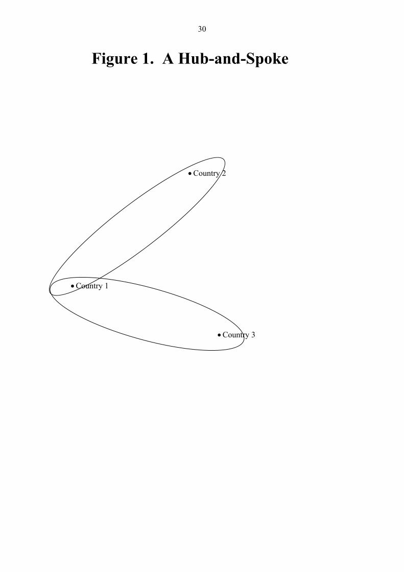
The natural way of depicting these intersections is to use Venn diagrams showing the

intersections of the sets of country membership of each RTA. This has been done by

Estevadeordal (2002) for the Americas and by Lloyd (2002, Figure 1) for the Asia-Pacific.

The hubs, single country or plurilateral, can be immediately identified as can the spokes,

single country or plurilateral. As a simple example, Figure 1 shows an example with three

18

countries. Country 1 is the hub as it has separate bilaterals with the two spoke countries,

Countries 1 and 2.

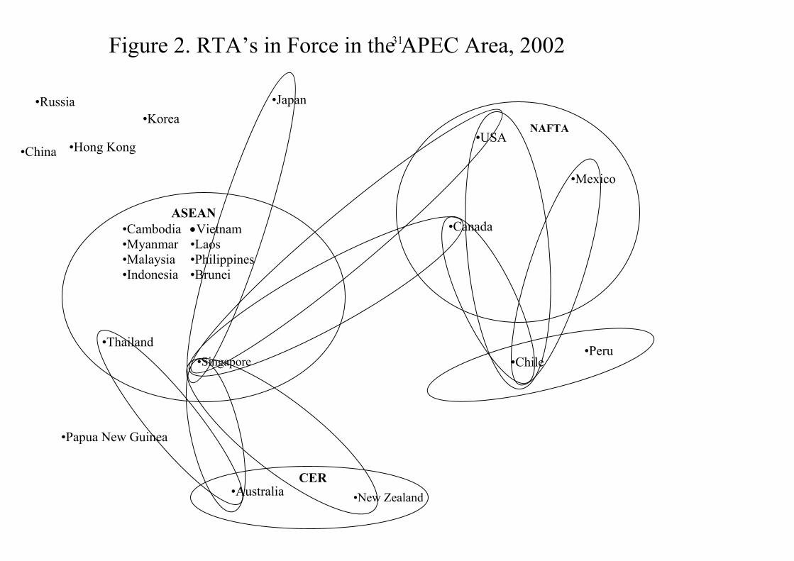
Figure 2 has an updated Venn diagram of the Asia-Pacific area. This area is taken to be the

21 countries of the APEC organisation. This area is of special interest because it is a

latecomer to RTAs compared to Europe and the Americas. In particular, Japan, China, South

Korea, Hong Kong, SAR and Taiwan staunchly followed a path of only multilateral (and

unilateral) liberalisation and eschewed RTAs until recently. To prevent the diagram from

becoming too big and unwieldy, the spoke arrangements with countries outside the APEC

area, the cross-regional agreements as they are called, are not depicted.

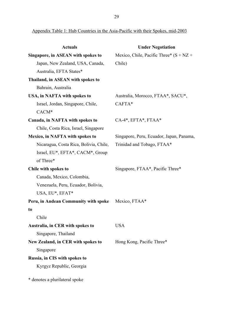
Hub-and-spoke arrangements in the Asia-Pacific, including cross-regionals, are listed in

Appendix Table 1. In this area, a majority of the APEC countries are hubs or will be hubs if

current negotiations are completed. Most of these hubs will have more than two spokes.

Other APEC countries such as Japan, South Korea and Malaysia have a number of spoke

arrangements under discussion and there are many other proposals involving the APEC

countries that have been officially mooted. None of the hubs are plurilaterals, however,

ASEAN as a party is now having official discussions with China and Japan and Korea - the

so-called ASEAN+3 proposal. Some of the spokes are plurilateral.

Thus, the Asia-Pacific is following the pattern in other areas. More countries are joining

RTAs, more hubs are emerging, the average number of spokes is increasing and some of the

spokes are plurilaterals.

A hub-and-spokes arrangement creates two layers of discrimination. Spokes have less

market access than the hub as the hub enjoys preferential access to all spokes but a spoke has

preferential access to the hub only and, conversely for import trade, a hub gets unrestricted

imports from all spokes whereas each spoke gets unrestricted imports only from its spoke

partner sources. When two or more hub-and-spoke arrangements themselves intersect, the

discrimination is multi-layered.

Multiple layers of discrimination do not fundamentally change the economics of trade

discrimination. For countries that are spokes the effects are the same as in an a non-

intersecting RTA, except that its preferential access to its partner’s markets is now shared

19

with competitors from another country or countries. For a hub country, tariff administration

is more complex as there are three (or more) columns in the tariff structure. For importers,

there are multiple sets of rules of origin that may have rules relating to cumulation across

countries and the treatment of outsourced inputs that can be extremely complex and costly to

conform to.

Two-layered discrimination provides incentives for the enlargement of pre-existing RTAs

and the coalescence of RTAs when there are intersections between them. (For some

discussion of the dynamics of RTAs, see Lloyd, 2002.) The intersections are concentrated in

Europe and the Americas and plainly RTAs in these two continents have been coalescing for

some time and continue to do so. There are distinct signs of the same process in East Asia.

The pattern of coalescence is consistent with the hypothesis that spoke countries seek to

equalise their preferential access with that of hub countries. This has occurred in both the

ASEAN and CER areas. Indeed, most current and prospective bilaterals now involve a party

that is a spoke to another party that is a hub. However, a defensive reaction may not be the

sole explanation in such cases. It also notable that many of the partners in bilaterals now

being negotiated or broached are countries that have a strategy of seeking bilaterals with

significant willing trading partners.

One possible outcome is the tripolar world in which there is one large bloc of freely trading

countries in Europe, one in the Americas and one in Asia. It seems highly likely that there

will be three large poles within a few years with each pole having one agreement or a number

of linked agreements that yield substantially free trade among a large number of countries,

with relatively few connections across these polar groups by means of cross-polar RTAs.

A tripolar outcome would provide a substantial liberalisation of world trade. It would be a

significant step towards global free trade. The large number of countries within each pole

would greatly reduce the concerns of the members of the polar region over trade diversion.

But there is an obvious danger. Any country left out of the poles would suffer heavy

discrimination against it and a deterioration in its terms of trade. Similarly, any country in

one of the poles but having major markets in another pole would also suffer heavy

discrimination.

20

The set of countries outside the major RTAs could include some Developing Countries,

especially those that are outside the poles geographically. Most of the plurilateral RTAs with

a larger number of members involve only developed countries and most bilaterals are

between developed countries or in a few cases between a developed and a developing

country; examples of the latter are the agreements Mexico has with the EU and EFTA

countries. Most of the hubs are developed countries. When the larger size of the markets in

developed countries and especially the US and the EU is taken into account, there is no doubt

that the increase in market access resulting from RTAs has gone overwhelmingly to

developed countries and not to developing countries.10 The one significant exception among

the developing countries appears to be Mexico which has secured mostly free access to its

major markets in both North America and Europe. This picture will change substantially if

and when the negotiations for the FTAA and the negotiations between the EU and

Developing African, Caribbean and Pacific countries are completed.

Of greatest concern, none of the bilaterals links a Least Developed Country to a Developed

Country. Very few LDCs are members of RTAs with other Developing Countries.

Myanmar, Laos and Cambodia are members of ASEAN that contains Singapore, a

Developed country, but ASEAN is mainly an RTA among Developing and LDC countries.

4. Effects of RTAs on Multilateral Trade Liberalisation

The growth of RTAs may affect the rate of multilateral liberalisation in two ways

• it may affect the pace of liberalisation from multilateral trade negotiations, and

• it may affect the pace of unilateral liberalisations (that are of course made by members

of the WTO on an MFN basis).

The effect of regionalism on the rate of multilateral negotiations is usually regarded as the big

issue. Does the formation of bilateral agreements have a positive or a negative effect on

multilateral trade negotiations? This has been called the “building block or stumbling block”

debate.

There is a literature in which the effects that RTAs may have on the incentives to pursue

multilateral liberalisation are modelled. Again, the results are ambiguous. The outcome

21

depends on whether one adopts a welfare-maximising or a political objective, on the height

and structure of initial tariff levels and many other variables. (For recent reviews, see

Panagariya, 1999 and Schiff and Winters, 2003, chapter 8.)

The actual record has been examined many times, including detailed examinations by the

OECD (1995), the WTO (1995) itself and the World Bank (2000). The answer commonly

given by earlier studies is that the formation of RTAs did not slow down multilateral

liberalisation.

However, it is possible that the recent explosion of RTAs and the new patterns emerging may

change this relationship. After the WTO Ministerial Conference in Cancún, both the US and

the EU declared that their priority is now with the completion of bilateral and regional trade

negotiations. Countries that are seeking RTAs with these super-hubs may also change their

priorities.

There is evidence too that the formation of larger continent-based RTA groups is changing

the stance that countries adopt on some issues in the multilateral negotiations. As one

example, a group of 22 Developing Countries (G-22) played a major role in the multilateral

negotiations at Cancún. They pressed for measures that would benefit Developing Countries

as a group and in particular adopted a very tough stance towards the EU and the US on farm

support and protection. Since the Ministerial Conference, six American Hemisphere

countries have withdrawn from the group. All of these are in the process of negotiating the

FTAA with the US. Similarly, at the APEC Economic Leaders’ Meeting in Bangkok later in

October, Australia supported the resolution agreeing to the use of the framework text tabled

in Cancún by the Chair of the General Council, the so-called Debrez text. This contained

words derived from the EU-US accord on agriculture that would achieve a very limited

liberalisation of agricultural trade and which appears to be at odds with the strong stance

Australia had previously taken on agricultural trade reform. At the time Australia was

entering the critical phase of the negotiations with the US over a free trade agreement.

In relation to possible new areas of rules such as investment, competition and preferential

rules of origin, many of these have been pioneered by RTAs the scope of the rules of which

go well beyond those of the WTO, that is, they are WTO-plus. However, the style of RTAs

with respect to these new areas differs greatly. Sampson and Woolcock (2003) call this

22

“regulatory regionalism”. There is increasing evidence that the EU and the US are using

their expanding networks of EU- and US- connected RTAs to form coalitions to advance the

EU’s and the US’s views of the forms that these new rules may take in the WTO.

In regard to unilateral liberalisation, Article XXIV is non-prescriptive. It lays down the rule

that the “duties and other regulations of commerce …shall not be higher or more restrictive”

than the pre-existing levels in the case of a free trade area and, in the case of a customs union

“…shall not on the whole be higher or more restrictive”. This rule has prevented trade

barriers being raised against third countries. However, this rule has not been sufficient to

protect the interests of outside countries. Economic models reviewed in Section 1 above

show clearly that the relevant variable is not the height of MFN barriers but the amount of

trade with third countries that results after the formation of an RTA. For outside countries to

be generally no worse off requires a lowering of these MFN barriers.

What has happened in reality to the rate of unilateral liberalisation by countries joining

RTAs? The evidence is mixed. The ASEAN countries and the CER countries have engaged

in substantial unilateral trade liberalisation during the period of reduction of trade barriers

within their RTAs. Latin America too conforms to this pattern. Estevadeordal (2002, Figure

2) shows that the MFN rates declined almost as rapidly as average preferential rates in Latin

America over the period 1985 to 1997. In NAFTA, Mexico and to a lesser extent Canada

have lowered MFN rates unilaterally. However, this coincidence of reductions in both

preferential and MFN rates over time cannot be construed as regionalism encouraging

multilateral or unilateral reductions. The cause and effect could go either way. Or, most

plausibly, it could be that both are due to change induced by reform-minded governments that

pursued the unilateral and regional routes to trade liberalisation.

On the other hand, the US and EU, two large customs territories whose intra-area trade is

much more than 50 per cent of total world intra-RTA trade (WTO, 2001, Table A4), have not

made any significant reductions in trade barriers in the last two decades that were not part of

RTAs or were part of the Uruguay Round multilateral concessions.

23

5. Concluding remarks

The outcome of the growth of RTAs under the GATT/WTO system is that in the last 15 years

or so there has been a great increase in discrimination in world trade. With the growth of

more hubs and an increase in the numbers of spokes and the emergence of pluritaleral hubs

and spokes, there is a complex multi-layered pattern of discrimination. This pattern has

benefited developed countries predominantly and harmed some outside countries.

The most important thing that has to be said regarding this pattern is that GATT/WTO rules

relating to RTAs have been a failure, perhaps the biggest failure of all areas of rules in the

GATT/WTO. The Preamble to the GATT 1947 laid down two objectives of the organisation:

“the substantial reduction of tariffs and other barriers to trade” and “the elimination of

discriminatory treatment in international commerce”. This language is repeated in the

preamble to the Marrakesh Agreement. The objective relating to trade discrimination is

stronger than that relating to trade barriers as the former calls for their elimination. Under

Article XXIV, RTAs were envisaged as exceptions but they have become the rule. No doubt

possible reforms of these rules and their enforcement will be discussed in other sessions of

this conference.

24

FOOTNOTES

1 There is a partial equilibrium diagram that is still popularly used to explain the economic effects of trade diversion and trade creation; see, for example, Pomfret (1997, pp. 182-185) and Schiff and Winters (2003, pp. 54-56). The diagram was devised by Johnson (1960). It is a partial equilibrium analogue of the general equilibrium expression in Equation (3). This expresses the total effect as the sum of the “trade diversion” and “trade creation” effects. However, the “trade creation” effect is the sum of a production and a consumption effect, and there is no extra-union change in the terms of trade by assumption. This Johnsonian interpretation of the “trade creation” effect cannot be regarded as a terms of trade effect or a trade volume effect. It is a money metric of aggregate welfare change, obtained by summing the welfare triangles and rectangle. 2 A related expression has been obtained by other authors. Ohyama used the Hicks criterion of potential real income change to get an expression similar to that in Equation (2). Panagariya (1997) used an expression equivalent to the trade expenditure function to obtain a marginal change in utility that was the sum of these effects. Baldwin and Venables (1995), derive an expression which contains additional effects, imperfect competition and scale effects and an increase in the variety of goods, and with capital accumulation and economic growth effects (see section 2). 3 It is evident from Equation (2) that the sign of these changes has to be defined carefully. 4 The results of both Mundell and Riezman require regularity conditions but these are not unreasonable. 5 For a complete account of the widely used global data base, GTAP, see Dimaranan and McDougall (2002). For a graphical exposition of the accounting identities in the GTAP model, see Brockmeier (2001). 6 For a more complete discussion, see Lloyd and MacLaren (2002). 7 It is possible, however, to decompose the welfare change into a terms of trade effect and an allocative efficiency effect in order to gain a sense of the importance of the terms of trade effect in the overall change in welfare. 8 Wonnacott described a hub as arising from the decision of an outside country to form a bilateral agreement with only one member of a multi-member pre-existing RTA. The inside country is called the hub. This definition of a hub is too narrow. The general phenomenon is one of intersections between RTAs. 9 These are the 10 accession countries plus the three countries that did not proceed with accession, 12 agreements with Developing Countries in the Mediterranean and Africa already in force or being negotiated. The agreements with the accession countries will lapse when they become full members. This number does not include the 77 African, Caribbean and Pacific countries with which the EU is negotiating to replace non-reciprocal agreements with reciprocal FTAs. 10 One must be careful to interpret these trends. RTAs are voluntary associations among nations. Generally, Developing Countries have been slower to form RTAs than Developed Countries, either among themselves or with Developed countries. Furthermore, the RTAs they have formed have been much less comprehensive in terms of commodity coverage and instrument coverage, though this has changed recently in some areas, notably Latin America. This feature has made them less attractive to Developed Countries as partners.

25

REFERENCES

Baldwin, R. E. and A. J. Venables (1995) “Regional Economic Integration”, in, G. M.

Grossman and K. Rogoff (eds), Handbook of International Economics, Volume III,

North-Holland, Amsterdam.

Brockmeier, M. (2001 revised) A Graphical Exposition of the GTAP Model, GTAP

Technical Paper No. 8, Center for Global Trade Analysis, Department of Agricultural

Economics, Purdue University.

Brown, D. K., A. V. Deardorff and R. M. Stern (1992) “A North American Free Trade

Agreement: Analytical Issues and Computational Assessment”, The World Economy,

15, 11-29.

Brown, D. K., A. V. Deardorff and R. M. Stern (2003) “Multilateral, Regional and Bilateral

Trade: Policy Options for the United States and Japan”, The World Economy, 26,

803-828.

Dimaranaran, B. V. and R. A. McDougall (eds) (2002) Global Trade, Assistance, and

Production: The GTAP 5 Data Base, Center for Global Trade Analysis, Department of

Agricultural Economics, Purdue University.

Estevadeordal, A. (2002), “Traditional Market Access Issues in RTAs: An Unfinished

Agenda in the Americas?”, paper presented to the WTO Seminar on Regionalism and

the WTO, Geneva, 26 April 2002. This is available at the WTO website

http://www.wto.org.

Gehrels, F. (1956-57), “Customs Unions from a Single-Country Viewpoint”, Review of

Economic Studies, 49, 696-712.

Grinols, E. (1981), “An Extension of the Kemp-Wan Theorem on the Formation of Customs

Unions”, Journal of International Economics, 11, 259-266.

26

Haaland, J. and V. Norman (1992) “Global production effects of European integration”, in L.

A. Winters (ed.) Trade Flows and Trade Policy after ‘1992’, Cambridge University

Press, Cambridge.

Hertel, T. W., T. Walmsley and K. Itakura (2001) “Dynamic Effects of the “New Age” Free

Trade Agreement between Japan and Singapore”, GTAP Working Paper No. 15,

Center for Global Trade Analysis, Department of Agricultural Economics, Purdue

University.

Johnson. H. G. (1960), “The Economic Theory of Customs Unions”, Pakistan Economic

Review, 10, 14-30.

Kemp, M. C. and H. Y. Wan (1976), “An Elementary Proposition Concerning the Formation

of Customs Unions”, Journal of International Economics, 6, February, 95-98.

Lipsey, R. G. (1957), “The Theory of Customs Unions: Trade Diversion and Welfare”,

Economica, 24, 40-46.

Lipsey, R. G. and K. Lancaster (1956-57), “The General Theory of the Second Best”, Review

of Economic Studies, 24, 11-32.

Lloyd, P. J. (2002), “New Bilateralism in the Asia-Pacific”, The World Economy, 25, 1279-

1296.

Lloyd, P. J. and D. MacLaren (2002) “Measures of trade openness using CGE analysis”,

Journal of Policy Modeling, 24, 67-81.

Lloyd, P. J. and A. G. Schweinberger (1988), “Trade Expenditure Functions and the Gains

from Trade”, Journal of International Economics, 24, 275-97.

Meade, J. E. (1955), The Theory of Customs Unions, North Holland, Amsterdam.

Michaely, M. (1965), “On Customs Unions and the Gains from Trade”, Economic Journal,

75, 577-583.

27

Mundell, R. (1964), “Tariff Preferences and the Terms of Trade”, Manchester School, 32, 1-

13.

Ohyama, M. (1972), “Trade and Welfare in General Equilibrium “, Keio Economic Studies,

9, 37-73.

Ohyama, M. (2003), “The Economic Significance of the GATT/WTO Rules” in A.

Woodland (ed.), Economic Theory and International Trade: Essays in Honour of

Murray C. Kemp, Edward Elgar, Cheltenham.

Organisation for Economic Cooperation and Development (OECD) (1995), Regional

Integration and the Multilateral Trading System: Synergy and Divergence, OECD,

Paris

Panagariya, A. (1997), “The Meade Model of Preferential Trading: History, Analytics and

Policy Implications”, in B. Chen (ed.), International Trade and Finance: New

Frontiers for Research, Essays in Honor of Peter B. Kenen , Cambridge University

Press, New York.

Panagariya, A. (1999), “The Regionalism Debate: An Overview”, The World Economy, 22,

477-511.

Panagariya, A. and P. Krishna (2002), “On Necessarily Welfare-enhancing Free Trade

Areas”, Journal of International Economics, 57, 353-67.

Pomfret, R. (1997), The Economics of Regional Trading Arrangements, Clarendon Press,

Oxford.

Riezman, R. (1979), “A 3x3 Model of Customs Unions”, Journal of International Economics,

9, 341-354.

Sampson, G. and S. Woolcock (2003), Regionalism, Multilateralism and Economic

Integration, United Nations University Press, Tokyo.

28

Schiff, M. and A. Winters (2003), Regional Integration and Development, Oxford University

Press for the World Bank, Washington, D. C.

Scollay, R. and J. P. Gilbert (2001), New Regional Trading Arrangements in the Asia

Pacific?, Institute for International Economics, Washington, D. C.

Srinivasan, T. (1997), “The Common External Tariff of a Customs Union: Alternative

Approaches”, Japan and the World Economy, 9, 447-465.

Viner, J. (1950), The Customs Union Issue, Carnegie Endowment, New York.

Wonnacott, R. J. (1996), “Trade and Investment in a Hub-and-spoke System versus a Free

Trade Area”, The World Economy, 19 (3), 237-252.

World Bank (2000), Trade Blocs, Oxford University Press for the World Bank, Washington,

D. C.

World Trade Organisation (WTO) (1995), Regional Trading Arrangements and the World

Trading System, WTO, Geneva.

Young, L. M. and K. M. Huff (1997) “Free trade in the Pacific Rim: On what basis?”, in T.

W. Hertel (ed.) Global Trade Analysis: Modeling and Applications, Cambridge

University Press, New York.

29

Appendix Table 1: Hub Countries in the Asia-Pacific with their Spokes, mid-2003

Actuals Under Negotiation

Singapore, in ASEAN with spokes to

Japan, New Zealand, USA, Canada,

Australia, EFTA States*

Mexico, Chile, Pacific Three* (S + NZ +

Chile)

Thailand, in ASEAN with spokes to

Bahrain, Australia

USA, in NAFTA with spokes to

Israel, Jordan, Singapore, Chile,

CACM*

Australia, Morocco, FTAA*, SACU*,

CAFTA*

Canada, in NAFTA with spokes to

Chile, Costa Rica, Israel, Singapore

CA-4*, EFTA*, FTAA*

Mexico, in NAFTA with spokes to

Nicaragua, Costa Rica, Bolivia, Chile,

Israel, EU*, EFTA*, CACM*, Group

of Three*

Singapore, Peru, Ecuador, Japan, Panama,

Trinidad and Tobago, FTAA*

Chile with spokes to

Canada, Mexico, Colombia,

Venezuela, Peru, Ecuador, Bolivia,

USA, EU*, EFAT*

Singapore, FTAA*, Pacific Three*

Peru, in Andean Community with spoke

to

Chile

Mexico, FTAA*

Australia, in CER with spokes to

Singapore, Thailand

USA

New Zealand, in CER with spokes to

Singapore

Hong Kong, Pacific Three*

Russia, in CIS with spokes to

Kyrgyz Republic, Georgia

* denotes a plurilateral spoke

30

Figure 1. A Hub-and-Spoke

• Country 1

• Country 2

• Country 3

31Figure 2. RTA’s in Force in the APEC Area, 20

•USA

•Chile

•Russia •Korea

•Hong Kong

•Japan

•Singapore

•New Zealand•Australia CER

•Papua New Guinea

ASEAN •Cambodia •Vietnam •Myanmar •Laos •Malaysia •Philippines •Indonesia •Brunei

•Canada

•Thailand

NA

•China

02

•Peru

•Mexico

FTA