The CAPM Strikes Back? An Investment Model with...
38
Transcript of The CAPM Strikes Back? An Investment Model with...

The CAPM Strikes Back?
An Investment Model with Disasters
Hang Bai1 Kewei Hou1 Howard Kung2 Lu Zhang3
1The Ohio State University
2London Business School
3The Ohio State University
and NBER
Federal Reserve Bank of New York
September 17, 2015

IntroductionInsight
An investment model with disasters replicates:
The failure of the CAPM in capturing the value premium in
�nite samples in which disasters are not materialized;
The relative success of the CAPM in samples in which
disasters are materialized

IntroductionLiterature
Early quantitative theories of cross-sectional asset pricing rely on
single-factor models:
Gomes, Kogan, and Zhang (2003); Carlson, Fisher, and
Giammarino (2004); Zhang (2005); Cooper (2006)
Recent quantitative theories introduce two-shock models:
Ai and Kiku (2013); Kogan and Papanikolaou (2013); Belo,
Lin, and Bazdresch (2014); Koh (2014)
Prior disaster models:
Rietz (1988); Barro (2006, 2009); Barro and Ursua (2008);
Gourio (2012); Gabaix (2012); Wachter (2013)

Outline
1 Stylized Facts
2 The Model
3 Failing the CAPM
4 The Beta Anomaly

Outline
1 Stylized Facts
2 The Model
3 Failing the CAPM
4 The Beta Anomaly

Stylized FactsThe CAPM regressions for the b/m deciles, July 1963�June 2014
Fama and French (1992, 1993)
L 2 3 4 5 6 7 8 9 H H−Lm 0.42 0.52 0.55 0.55 0.54 0.59 0.68 0.71 0.79 0.93 0.51tm 2.00 2.72 2.95 2.89 2.97 3.25 3.81 3.88 4.07 3.91 2.75α −0.12 0.01 0.06 0.06 0.08 0.13 0.24 0.27 0.32 0.39 0.51tα −1.28 0.15 0.92 0.57 0.83 1.45 2.27 2.28 2.92 2.50 2.26β 1.06 1.01 0.98 0.99 0.91 0.93 0.88 0.88 0.94 1.07 0.01tβ 40.79 46.28 34.55 29.35 27.50 28.34 22.89 17.53 20.85 15.44 0.07R2 0.86 0.92 0.90 0.87 0.83 0.85 0.78 0.76 0.76 0.66 0.00

Stylized FactsThe CAPM regressions for the b/m deciles, July 1926�June 2014
Ang and Chen (2007)
L 2 3 4 5 6 7 8 9 H H−Lm 0.57 0.68 0.68 0.68 0.73 0.76 0.77 0.92 1.03 1.09 0.52tm 3.24 4.09 4.05 3.67 4.12 4.04 3.86 4.43 4.36 3.82 2.60α −0.09 0.06 0.05 −0.01 0.08 0.07 0.05 0.18 0.21 0.14 0.23tα −1.27 1.20 0.89 −0.13 1.02 0.93 0.58 1.93 1.83 0.94 1.18β 1.00 0.95 0.97 1.06 1.00 1.05 1.09 1.14 1.27 1.45 0.45tβ 47.76 28.52 59.63 20.06 27.74 16.04 16.14 15.40 13.46 13.38 3.52R2 0.90 0.92 0.92 0.90 0.89 0.87 0.84 0.82 0.79 0.72 0.14

Stylized FactsThe value premium vs. MKT, July 1926�June 2014
−40 −20 0 20 40−40
−20
0
20
40
60
80
28Nov
29Oct
30Jun31May
31Jun
31Sep
31Dec
32Apr
32May
32Jul
32Aug
32Oct33Feb
33Apr
33May
33Jun33Aug
34Jan
37Sep
38Mar
38Apr
38Jun
39Sep
40May 74Oct
75Jan76Jan
80Mar87Jan87Oct
98Aug
08Oct
The market excess return
The v
alu
e p
rem
ium
−40 −20 0 20 40−40
−20
0
20
40
60
80
The market excess return
The v
alu
e p
rem
ium

Stylized FactsLarge swings in the stock market and the value premium
MKT H−L MKT H−L
November 1928 11.79 −0.41 August 1933 12.03 4.92October 1929 −20.07 7.57 January 1934 12.63 34.10June 1930 −16.25 −3.54 September 1937 −13.57 −10.90May 1931 −13.16 −3.09 March 1938 −23.80 −22.67June 1931 13.75 14.80 April 1938 14.49 8.76September 1931 −29.07 −5.03 June 1938 23.77 15.22December 1931 −13.42 −16.73 September 1939 16.94 56.61April 1932 −17.98 −2.85 May 1940 −21.93 −15.49May 1932 −20.44 3.61 October 1974 16.10 −13.58July 1932 33.47 45.73 January 1975 13.66 19.70August 1932 36.41 69.99 January 1976 12.16 15.04October 1932 −13.09 −12.97 March 1980 −12.90 −9.02February 1933 −15.06 −7.45 January 1987 12.47 −2.98April 1933 37.93 22.41 October 1987 −23.24 −1.21May 1933 21.36 45.01 August 1998 −16.08 6.33June 1933 13.05 10.29 October 2008 −17.23 −11.93

Stylized FactsThe CAPM's general problem, the beta anomaly,July 1963�June 2014, Fama and French (2006)
L 2 3 4 5 6 7 8 9 H H−Lm 0.51 0.52 0.52 0.56 0.66 0.54 0.68 0.53 0.62 0.63 0.12tm 3.64 3.46 3.11 3.15 3.46 2.67 3.06 2.25 2.33 1.92 0.43α 0.22 0.17 0.11 0.12 0.17 0.02 0.10 −0.08 −0.06 −0.18 −0.40tα 2.03 1.75 1.32 1.39 1.89 0.22 1.17 −0.83 −0.47 −0.90 −1.48β 0.57 0.68 0.81 0.87 0.98 1.03 1.14 1.22 1.35 1.61 1.04tβ 12.29 16.79 19.13 20.74 27.23 30.22 46.72 41.42 34.60 30.04 11.41R2 0.54 0.68 0.77 0.79 0.86 0.86 0.88 0.86 0.84 0.78 0.43

Stylized FactsThe CAPM's general problem, the beta anomaly,July 1928�June 2014, Fama and French (2006)
L 2 3 4 5 6 7 8 9 H H−Lm 0.57 0.63 0.64 0.73 0.82 0.71 0.80 0.72 0.82 0.81 0.24tm 4.80 4.51 4.23 4.33 4.36 3.55 3.69 2.99 3.04 2.59 0.94α 0.21 0.17 0.12 0.14 0.16 0.01 0.04 −0.13 −0.11 −0.26 −0.47tα 2.68 2.18 2.04 2.37 2.29 0.11 0.54 −1.53 −1.09 −1.80 −2.40β 0.57 0.74 0.82 0.93 1.05 1.12 1.22 1.36 1.49 1.70 1.12tβ 22.94 29.62 35.56 40.62 41.07 40.12 46.51 36.08 26.55 40.59 18.46R2 0.67 0.81 0.85 0.88 0.90 0.90 0.91 0.90 0.88 0.85 0.58

Outline
1 Stylized Facts
2 The Model
3 Failing the CAPM
4 The Beta Anomaly

The ModelHighlights
Embedding disasters into a standard investment model:
Rare disasters in consumption (productivity) growth
Asymmetric adjustment costs: Value �rms are more exposed
to disaster risk than growth �rms
Recursive preferences
In a sample without disasters, estimated betas only re�ect risk in
normal times, but the value premium is driven by disaster risk

The ModelRecursive utility
The pricing kernel:
Mt+1 = ι
(Ct+1
Ct
)− 1
ψ
U1−γt+1
Et
[U1−γt+1
]
1/ψ−γ1−γ

The ModelConsumption dynamics
Log consumption growth:
gct = g + gt
Normal states follow a discretized autoregressive process:
Five states: {g1, g2, g3, g4, g5}Transition matrix: pij ≡ Prob(gt+1 = gi |gt = gj):
P =
p11 p12 . . . p15p21 p22 . . . p25
......
. . ....
p51 p52 . . . p55

The ModelConsumption dynamics
Insert the disaster state, g0 = λD (disaster size < 0), and the
recovery state, g6 = λR (recovery size > 0)
Modify transition matrix:
P =
θ 0 0 . . . 0 1− θη p11 − η p12 . . . p15 0
η p21 p22 − η . . . p25 0...
......
. . ....
...
η p51 p52 . . . p55 − η 0
0 (1− ν)/5 (1− ν)/5 . . . (1− ν)/5 ν
η: disaster probability; θ: disaster persistence; ν: recoverypersistence

The ModelFirms, technology
Operating pro�ts:
Πit = (XtZit)1−ξK ξ
it − fKit
Aggregate productivity growth:
gxt = g + φgt
Firm-speci�c productivity:
zit+1 = (1− ρz)z + ρzzit + σzeit+1
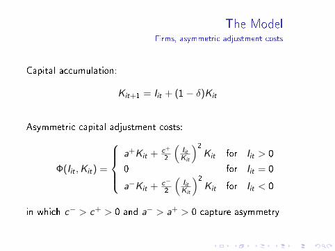
The ModelFirms, asymmetric adjustment costs
Capital accumulation:
Kit+1 = Iit + (1− δ)Kit
Asymmetric capital adjustment costs:
Φ(Iit ,Kit) =
a+Kit + c+
2
(IitKit
)2Kit for Iit > 0
0 for Iit = 0
a−Kit + c−
2
(IitKit
)2Kit for Iit < 0
in which c− > c+ > 0 and a− > a+ > 0 capture asymmetry

The ModelFirms, value maximization
Source of funds constraint:
Dit = Πit − Iit − Φ(Iit ,Kit)
Value maximization:
Vit = max{χit}
(max{Iit}
Dit + Et [Mt+1V (Kit+1,Xt+1,Zit+1)] , sKit
),
in which s ≥ 0 is the liquidation value parameter
Entry and exit, delisting return, reorganizational costs

Outline
1 Stylized Facts
2 The Model
3 Failing the CAPM
4 The Beta Anomaly

Failing the CAPMCalibration, preferences
Parameters Value Description
ι 0.99035 Time discount factorγ 5 The relative risk aversionψ 1.5 The elasticity of intertemporal substitution

Failing the CAPMCalibration, consumption dynamics
Parameters Value Description
g 0.019/12 The average consumption growthρg 0.6 The persistence of consumption growthσg 0.0025 The conditional volatility of consumption growth
η 0.028/12 The disaster probabilityλD −0.0275 The disaster sizeθ 0.9141/3 The disaster persistenceλR 0.0325 The recovery sizeν 0.95 The recovery persistence

Failing the CAPMThe impulse response of log consumption to a disaster shock
mimics that in Nakamura, Steinsson, Barro, and Ursua (2013)
0 5 10 15 20 25−0.25
−0.2
−0.15
−0.1
−0.05
0

Failing the CAPMCalibration, technology
Parameters Value Description
ξ 0.65 The curvature parameter in the production functionδ 0.01 The capital depreciation ratef 0.005 Fixed costs of productionφ 1 The leverage of productivity growth
z −9.75 The long-run mean of log �rm-speci�c productivityρz 0.985 The persistence of log �rm-speci�c productivityσz 0.5 The conditional volatility of log �rm-speci�c productivity
a+ 0.035 Upward nonconvex adjustment costsa− 0.05 Downward nonconvex adjustment costsc+ 75 Upward convex adjustment costsc− 150 Downward convex adjustment costs
s 0 The liquidation value parameterκ 0.25 The reorganizational cost parameter
R −0.425 The delisting return

Failing the CAPMThe CAPM regressions for the b/m deciles, no-disaster samples
G 2 3 4 5 6 7 8 9 V V−Gm 0.77 0.76 0.75 0.75 0.75 0.77 0.80 0.85 0.95 1.21 0.45tm 18.58 18.43 18.09 17.98 18.11 18.57 19.32 20.52 22.55 24.99 7.10α −0.01 −0.02 −0.06 −0.11 −0.10 −0.08 −0.02 0.08 0.23 0.46 0.47tα −0.07 −0.24 −0.73 −1.26 −1.24 −0.95 −0.18 0.99 2.83 5.02 3.71β 0.95 0.96 1.00 1.05 1.05 1.05 1.00 0.95 0.89 0.92 −0.03tβ 11.07 10.87 11.32 11.98 11.89 11.88 11.47 10.95 9.85 9.00 −0.24R2 0.11 0.12 0.12 0.14 0.14 0.13 0.13 0.11 0.10 0.08 0.00

Failing the CAPMThe CAPM regressions for the b/m deciles, disaster samples
G 2 3 4 5 6 7 8 9 V V−Gm 0.74 0.74 0.73 0.74 0.75 0.77 0.81 0.86 0.96 1.19 0.45tm 13.83 13.61 13.43 13.24 13.15 13.07 13.10 13.07 13.17 13.61 5.83α 0.08 0.06 0.04 0.01 −0.00 −0.03 −0.05 −0.09 −0.13 −0.13 −0.21tα 1.38 1.09 0.76 0.32 −0.08 −0.53 −0.82 −1.15 −1.40 −1.38 −1.72β 0.82 0.85 0.87 0.90 0.94 1.00 1.08 1.19 1.37 1.64 0.82tβ 18.82 23.74 28.64 33.03 33.72 30.60 26.47 20.63 16.00 18.05 6.82R2 0.45 0.47 0.49 0.50 0.52 0.55 0.57 0.60 0.64 0.65 0.24

Failing the CAPMValue is more exposed to disaster risk than growth
−20−10
0
0
10
20
0
10
20
30
zCapital −20−10
0
0
10
20
0
10
20
30
zCapital

Failing the CAPMImpulse responses of risk and risk premiums for value and
growth deciles to a disaster shock
0 5 10 15 20 250
0.05
0.1
0.15
0.2
0.25
0.3
0.35
0.4
0 5 10 15 20 25−1
0
1
2
3
4
5

Failing the CAPMNonlinearity in the CAPM regressions
−20 0 20 40 60−40
−20
0
20
40
60
The v
alu
e p
rem
ium
The market excess return

Failing the CAPMNonlinearity in the pricing kernel
−20 0 20 40 600
5
10
15
20
25
The p
ricin
g k
ern
el
The market excess return

Failing the CAPMComparative statics
λD θ η ν λR
−0.025 −0.03 0.955 0.985 0.13% 0.33% 0.935 0.965 2.75% 3.75%Disaster samples
m 0.34 0.55 0.29 0.47 0.42 0.46 0.46 0.43 0.45 0.44tm 4.78 6.75 4.49 5.62 5.72 5.78 5.94 5.61 5.83 5.70α −0.22 −0.20 −0.21 −0.16 −0.21 −0.21 −0.20 −0.22 −0.21 −0.21tα −1.98 −1.51 −2.08 −1.33 −1.60 −1.89 −1.66 −1.80 −1.75 −1.78β 0.77 0.86 0.74 0.77 0.79 0.86 0.85 0.78 0.85 0.81tβ 6.65 7.11 6.56 7.39 6.01 7.80 6.74 6.75 6.74 7.04
No-disaster samples
m 0.33 0.54 0.28 0.55 0.42 0.46 0.45 0.43 0.44 0.45tm 5.63 8.08 5.24 7.89 6.74 7.29 7.09 6.90 6.99 7.06α 0.24 0.71 0.07 0.86 0.43 0.50 0.49 0.45 0.47 0.47tα 2.14 4.96 0.67 5.66 3.38 3.97 3.88 3.52 3.72 3.77β 0.12 −0.19 0.32 −0.33 −0.02 −0.05 −0.05 −0.02 −0.04 −0.04tβ 0.89 −1.35 2.56 −2.32 −0.13 −0.35 −0.41 −0.19 −0.31 −0.34

Failing the CAPMComparative statics
a+ a− c+ c− f
0.025 0.045 0.035 0.065 50 100 100 200 0 0.015Disaster samples
m 0.48 0.29 0.25 0.47 0.37 0.49 0.39 0.46 0.47 0.40tm 6.57 3.75 3.73 5.97 4.64 6.59 5.25 5.90 6.30 4.86α −0.25 −0.23 −0.21 −0.23 −0.24 −0.20 −0.21 −0.22 −0.21 −0.22tα −1.91 −2.05 −1.66 −1.82 −2.04 −1.61 −1.82 −1.80 −1.71 −1.89β 0.96 0.64 0.61 0.89 0.73 0.90 0.76 0.85 0.87 0.75tβ 6.42 6.19 4.32 6.77 7.23 6.57 6.57 6.85 6.61 7.25
No-disaster samples
m 0.45 0.28 0.22 0.46 0.38 0.49 0.39 0.46 0.45 0.40tm 8.48 4.24 3.84 7.32 5.54 8.42 6.35 7.29 7.78 5.81α 0.63 0.14 0.26 0.49 0.27 0.62 0.41 0.49 0.54 0.31tα 5.39 1.10 2.16 3.83 1.98 5.12 3.27 3.89 4.42 2.31β −0.23 0.16 −0.04 −0.04 0.13 −0.17 −0.02 −0.04 −0.10 0.11tβ −1.71 1.20 −0.32 −0.31 0.96 −1.25 −0.15 −0.36 −0.77 0.76

Failing the CAPMComparative statics
s κ R γ ψ
0.15 0.3 0 0.5 −0.3 −0.55 3.5 6.5 1 2Disaster samples
m 0.20 −0.03 0.45 0.45 0.47 0.44 0.18 0.57 −0.06 0.51tm 2.95 −0.28 5.79 5.87 6.08 5.64 2.61 7.19 −2.67 5.74α −0.27 −0.35 −0.21 −0.21 −0.19 −0.23 −0.23 −0.11 −0.29 −0.18tα −2.72 −3.80 −1.72 −1.73 −1.58 −1.89 −2.48 −0.81 −10.00 −1.60β 0.63 0.48 0.82 0.83 0.83 0.83 0.75 0.67 1.74 0.67tβ 7.06 6.57 6.84 6.80 6.75 6.85 6.24 5.29 10.34 8.43
No-disaster samples
m 0.27 0.10 0.44 0.45 0.46 0.44 0.15 0.60 −0.07 0.50tm 4.37 1.68 7.07 7.11 7.27 7.03 3.18 8.47 −3.15 7.10α 0.34 0.20 0.47 0.47 0.48 0.47 −0.12 0.96 −0.31 0.82tα 2.78 1.74 3.68 3.69 3.76 3.65 −1.64 5.87 −11.70 5.23β −0.09 −0.13 −0.03 −0.03 −0.03 −0.03 0.51 −0.34 1.98 −0.30tβ −0.66 −1.01 −0.22 −0.23 −0.22 −0.25 4.35 −2.45 17.67 −2.27

Outline
1 Stylized Facts
2 The Model
3 Failing the CAPM
4 The Beta Anomaly

The Beta AnomalyDeciles formed on rolling market betas, disaster samples
L 2 3 4 5 6 7 8 9 H H−Lm 0.76 0.78 0.81 0.83 0.85 0.86 0.86 0.85 0.83 0.79 0.04tm 13.72 14.09 14.04 13.89 13.55 13.41 13.08 12.65 11.79 11.50 0.53α 0.04 0.06 0.06 0.04 0.01 −0.01 −0.04 −0.08 −0.16 −0.17 −0.21tα 0.69 1.29 1.17 0.82 0.29 −0.05 −0.49 −0.89 −1.45 −2.10 −1.73β 0.90 0.90 0.95 0.99 1.04 1.08 1.12 1.16 1.23 1.20 0.30tβ 19.75 25.57 33.62 34.40 31.60 25.92 21.23 18.56 15.11 17.35 2.49R2 0.53 0.53 0.54 0.55 0.56 0.57 0.58 0.59 0.60 0.61 0.06

The Beta AnomalyDeciles formed on rolling market betas, no-disaster samples
L 2 3 4 5 6 7 8 9 H H−Lm 0.80 0.82 0.84 0.85 0.85 0.86 0.84 0.82 0.79 0.74 −0.06tm 20.12 20.36 20.48 20.45 19.82 20.00 19.58 18.98 18.24 16.65 −0.93α 0.01 0.12 0.17 0.19 0.15 0.16 0.11 0.03 −0.09 −0.42 −0.44tα 0.16 1.55 2.15 2.28 1.75 1.88 1.30 0.39 −1.06 −4.98 −3.49β 0.97 0.86 0.82 0.82 0.86 0.86 0.90 0.97 1.08 1.43 0.47tβ 11.79 10.20 9.50 9.27 9.30 9.15 9.72 10.37 11.67 15.74 3.49R2 0.13 0.10 0.09 0.09 0.09 0.09 0.10 0.11 0.14 0.23 0.01

The Beta AnomalyMeasurement errors in rolling market betas

ConclusionSummary
An investment model with disasters replicates the failure of the
CAPM in capturing the value premium in no-disaster samples, and
its relative success in disaster samples
The beta anomaly largely due to measurement errors in pre-ranking
rolling betas
A �rst step in integrating the disaster literature with
investment-based asset pricing