The canopy conductance of a boreal aspen forest, … Copies of my papers...The canopy conductance of...

HYDROLOGICAL PROCESSESHydrol. Process. 18, 1561–1578 (2004)Published online in Wiley InterScience (www.interscience.wiley.com). DOI: 10.1002/hyp.1406

The canopy conductance of a boreal aspen forest, PrinceAlbert National Park, Canada

P. D. Blanken1* and T. A. Black2

1 University of Colorado at Boulder, Boulder, Colorado, USA2 University of British Columbia, Vancouver, British Columbia, Canada

Abstract:

Annual fluxes of canopy-level heat, water vapour and carbon dioxide were measured using eddy covariance both abovethe aspen overstory (Populus tremuloides Michx.) and hazelnut understory (Corylus cornuta Marsh.) of a boreal aspenforest (53Ð629 °N 106Ð200 °W). Partitioning of the fluxes between overstory and understory components allowed thecalculation of canopy conductance to water vapour for both species. On a seasonal basis, the canopy conductanceof the aspen accounted for 70% of the surface conductance, with the latter a strong function of the forest’s leafarea index. On a half-hour basis, the canopy conductance of both species decreased non-linearly as the leaf-surfacesaturation deficits increased, and was best parameterized and showed similar sensitivities to a modified form of theBall–Berry–Woodrow index, where relative humidity was replaced with the reciprocal of the saturation deficit. Thenegative feedback between the forest evaporation and the saturation deficit in the convective boundary layer variedfrom weak when the forest was at full leaf to strong when the forest was developing or loosing leaves. The couplingbetween the air at the leaf surface and the convective boundary layer also varied seasonally, with coupling decreasingwith increasing leaf area. Compared with coniferous boreal forests, the seasonal changes in leaf area had a uniqueimpact on vegetation–atmosphere interactions. Copyright 2004 John Wiley & Sons, Ltd.

KEY WORDS BOREAS; canopy resistance; Corylus cornuta; evaporation; Populus tremuloides; transpiration

INTRODUCTION

The boreal forest is comprised primarily of coniferous species well adapted to the harsh environment. In thesouthern boreal forest, however, deciduous aspen (Populus tremuloides Michx.) with a hazelnut understory(Corylus cornuta Marsh.) forests are found, with extensive aspen stands comprising 13Ð5% of the southernboreal forest, and another 15Ð4% covered by mixed deciduous forests (Hall et al., 1997). As a result ofthe seasonal changes in leaf area, aspen–hazelnut forests display dramatic seasonal patterns in their energy(Blanken et al., 2001) and carbon balances (Black et al., 2000), in comparison to their coniferous counterparts.

This research was part of the BOreal Ecosystem–Atmosphere Study (BOREAS), a multiscale, multidisci-pline field-based study with the objective of improving our understanding of the role of the boreal forest inEarth’s climate system (see Sellers et al., 1995), through (but not exclusively) improving climate–biospheremodels. Water vapour and carbon dioxide both play crucial roles in the climate system, and both are exchangedbetween vegetation and the atmosphere through leaf stomata. The extent to which stomata conduct watervapour and carbon dioxide at the canopy scale (i.e. canopy conductance, gc) depends on the amount of leavesand several environmental controls (Blanken, 2002). Given the pronounced seasonal change in the amountof leaves in a deciduous aspen forest, in addition to the presence of a lush deciduous understory, we weremotivated to question: Which variables are important in controlling gc? How is gc best calculated from these

* Correspondence to: P. D. Blanken, Department of Geography and Program in Environment Studies, University of Colorado at Boulder,260 UCB, Boulder, Colorado 80309-0260, USA. E-mail: [email protected]

Received 28 October 2002Copyright 2004 John Wiley & Sons, Ltd. Accepted 17 April 2003

1562 P. D. BLANKEN AND T. A. BLACK

variables? Do the overstory and understory need to be treated separately (i.e. a two-layered model) in thisopen-canopied boreal forest?

Working at the canopy level, we present a study addressing some of these issues. For the gc of the forest asa whole, and both the aspen overstory and hazelnut understory individually, the objectives of this paper areto: (i) quantify the diurnal and seasonal patterns of gc; (ii) determine the processes controlling gc includingfeedback with the convective boundary layer and; (iii) assemble these processes in a framework suitable forapplication in land surface modelling schemes.

SITE DESCRIPTION

Located in Prince Albert National Park, Saskatchewan, Canada (53Ð629 °N 106Ð200 °W), the study site liesat the southern limit of the North American boreal forest. An even-aged 70-year-old aspen stand with amean height of 21Ð5 m, a diameter at the 1Ð3-m height of 20 cm (1 SD š 4Ð5 cm) and a stem density of 830stems ha1 developed after fire. Aspen leaves were confined to the top 5–6 m of the canopy, and canopyclosure averaged 89% (Sellers et al., 1994). The hazelnut understory had a mean height of 2Ð0 m, with foliagedistributed throughout. This homogeneous aspen–hazelnut cover extended for at least 3 km around the studysite, and is typical of the southern edge of boreal forest in central Canada especially, where 20–40% ofCanada’s aspen stands are located (Peterson and Peterson, 1992). More than 71% of Canada’s aspen/poplardominant stands are found in the boreal forest region.

Of the daytime mean above-aspen photosynthetic photon flux density (Qp#, 57% and 20% reached thehazelnut level, before and after aspen leaf development, respectively. Optical measurements (model LAI-2000, Li-Cor Inc., Linclon, NB) gave maximum leaf-area indexes (leaf area index, al) of 2Ð3 (aspen) and 3Ð3(hazelnut) m2 m2, reached by mid-July. Based on these measurements, we define the full-leaf period as 1June to 7 September 1994. The mean annual 1994 air temperature of 1Ð2 °C with 488 mm precipitation whencompared to the long-term daily mean air temperature of 0Ð4 °C with 467 mm of precipitation (recorded atWaskesiu Lake, 53Ð917 °N 106Ð083 °W, between 1971–1994 and 1971–1995, temperature and precipitation,respectively) showed that 1994 was a relatively warm and wet year.

MATERIALS AND METHODS

The vertical exchanges of latent heat (E), sensible heat (H) and CO2 (Fc both above the aspen andhazelnut were measured half-hourly by eddy covariance. This non-obtrusive, direct method calculates fluxesas the covariance between the instantaneous vertical wind speed (w) and the instantaneous scalar quantity(s) covws D w0s0 D w ws s where primes denote deviations from the block-averaged half-hourmean (overbars). Vertical wind speed was measured by three-dimensional sonic anemometers (model DAT-310, Kaijo-Denki, Tokyo, Japan above the aspen; model 1012R2A Solent, Gill instruments, Lymington,UK above the hazelnut). Water vapour and CO2 mole fractions were measured by infrared gas analysers(model 6262, Li-Cor Inc., Lincoln, NE), with air drawn through heated sampling tubes at flow rates of6Ð5 (aspen) and 8Ð0 L min1 (hazelnut) by diaphragm pumps. At the aspen level, signals were sampled at100 Hz, filtered with a low-pass 50-Hz cut-off frequency RC filter, then reduced to 20 Hz using a five-point block average (this effectively reduced signal aliasing and rejected 60-Hz AC power line noise). Atthe hazelnut level, signals were sampled at 20 Hz with an analogue cut-off frequency of 10 Hz. Instrumentswere supported by two towers at heights (z) of 39 m (17Ð5 m above the aspen canopy) and 4 m abovethe ground (2 m above the hazelnut canopy). Turbulence intensity (ratio of the standard deviation of thevertical wind speed, w, to the mean horizontal wind speed, u: w/u) increased from 0Ð26 at z D 39 mto 0Ð69 at z D 4 m, owing to the large decrease in the within-canopy u (15% of that above the aspen)relative to w. Despite these changes, within-canopy turbulence still obeyed the standard scaling laws(Blanken et al., 1998). Energy balance closure, or how well we measured all of the energy balance terms,

Copyright 2004 John Wiley & Sons, Ltd. Hydrol. Process. 18, 1561–1578 (2004)

BOREAL ASPEN CANOPY CONDUCTANCE 1563

was assessed by a linear regression of the turbulent flux terms (E C H) against the available energy(Ra; see Blanken et al. (1997) for details on Ra measurements). Using 24-h means (all in W m2), theregression equations were E C H D 0Ð98Ra C 3Ð4r2 D 0Ð93 and E C H D 1Ð01Ra C 1Ð3r2 D 0Ð88), for39-m and 4-m heights, respectively. Using the 1/2-hour data, the regression equations (all in W m2,were E C H D 0Ð87Ra C 14Ð2r2 D 0Ð93) and E C H D 0Ð84Ra C 5Ð2r2 D 0Ð77), for 39-m and 4-m heights,respectively. The slopes of the regressions being close to 1 show that we did a satisfactory job of measuringthe energy balance, even beneath the aspen canopy. Black et al. (1996) and Blanken et al. (1998) give furtherdetails on the eddy covariance instrumentation and turbulent flux measurements.

Soil E was measured using two thin-walled plastic 15-cm diameter by 15-cm deep lysimeters. The forestfloor was fairly homogeneous, covered only by leaf litter (no moss or lichen), and close agreement betweenthe two lysimeters implied that they represented a reasonable estimate of E from the soil. During a 15-dayrain-free period in mid-summer, the lysimeters were manually weighed every 2 h to the nearest 0Ð1 g (modelP3, Mettler Instrument Corp., Princeton, NJ) with the soil replaced after 5 days. The leafed-period meanE(soil) was 23% of E(4 m), and this ratio was used to estimate E(soil) throughout this period. During thepre-leaf period, E(soil) was assumed to equal the pre-leaf mean of 90% of E(4 m). Soil-water evaporationwas consistently much smaller than evaporation from the stand (5% annually) because of shading provided bythe high leaf area of the overstory canopies, and measurements of soil temperature using a hand-held infraredthermometer revealed little variation, indicating that E(soil) probably did not vary much within the area ofthe E(4 m) flux footprint.

The upwind source area or distance contributing to the flux measurements was calculated using the solutionsto the diffusion equations given by Schuepp et al. (1990). The upwind distance where the above-aspen fluxmeasurements were most sensitive was 123 m away from the tower during periods of neutral atmosphericstability, contracting to 98 m during typical daytime unstable atmospheric conditions. Above the hazelnut,these distances were 14 (neutral stability) and 9 m (daytime unstable). Eighty per cent of the flux originatedwithin 120 and 1190 m upwind of the towers (above hazelnut and aspen, respectively) during periods ofneutral atmospheric stability.

Canopy conductance, gc, was calculated using a rearranged form of the Penman–Monteith equation

1/gc D[(

s

)ˇ 1

]1/ga C acp

Da

E1

where s is the rate of increase of saturation vapour pressure with air temperature, is the psychrometricconstant, ˇ is the Bowen ratio (H/E), ga is the aerodynamic conductance, a and cp are density andspecific heat of air, respectively, and Da is the saturation deficit. The aerodynamic conductance was expressedas 1/ga D 1/gb C 1/ge where gb and ge are the canopy boundary layer and eddy diffusive conductances,respectively. The boundary layer conductance was calculated as 1/gb D B1/uŁ where uŁ is the frictionvelocity calculated from the eddy-covariance measured momentum flux and B1 is the dimensionless sublayerStanton number, which is proportional to the ratio of heat transfer to thermal capacity (Owen and Thompson,1963; Verma, 1989; Monteith and Unsworth, 1990). The eddy diffusive conductance was calculated as1/ge D u/u2

Ł.Measuring fluxes above and below the aspen canopy allowed us to isolate the flux contributions from

each canopy, thus calculate gc individually from both the aspen and hazelnut canopies, or the forest as awhole. Such partitioning of turbulent fluxes between two successive levels in forests has been accomplishedsuccessfully by others (e.g. Lee and Black, 1993; Baldocchi et al., 1997; Kelliher et al., 1999; Wilson andMeyers, 2001). Intercomparison of the two eddy covariance systems prior to vertical separation revealedfluxes calculated by each were consistently within 5% of each other. Above both canopies, the magnitudesof E and H were independent of wind direction, indicating relatively homogeneous canopies within the fluxfootprints.

Calculation of the aspen gc used Da and ga measured at z D 39 m, E(aspen) D E (39 m)—E(4 m), andH(aspen) D H39 m)—H4 m). For the hazelnut gc, we used Da and ga measured at z D 4 m, E(hazelnut) D



E(4 m)—E(soil), and H(hazelnut) D H(4 m)—H(soil). Calculation of the conductance for the surface asa whole (including aspen transpiration, hazelnut transpiration and soil water evaporation) is designated gS

and was determined with all variables measured at z D 39 m. The daytime mean gc was calculated using thedaytime means of all the variables when Qp# (39 m) exceeded 200 µmol m2 s1 and only when the canopieswere dry as indicated by leaf wetness sensors (model 237, Campbell Scientific Inc., Logan, UT), typicallywithin 1-h, after rainfall.

Variables showing a relationship with gc often need to be defined at the leaf surface (subscript 0) ratherthan in the ambient atmosphere (subscript a) (Bunce, 1985). Hence, the temperature (T0, saturation deficit(D0, relative humidity (h0 and CO2 mole fraction (c

0, all at the big-leaf surface, were calculated as

T0 D TS C [1/acp]H/ga 2

D0 D E/gc[/acp] 3

h0 D 1 D0/eŁT0 4

c0 D c

a An/ga 5

where ca is the CO2 mole fraction in the ambient air outside the leaf boundary layer, eŁ is the saturation

vapour pressure at T0, and TS is the surface temperature measured by two infrared thermometers (models 4000,Everest Interscience Inc., Tucson, AZ). If conditions at the aspen big-leaf surface were required, then variablesmeasured at z D 39 m were used in Equations (2) through to (5) with H(aspen) and E(aspen). Conditionsat the hazelnut big-leaf surface used variables measured at z D 4 with H(hazelnut) and E(hazelnut).The canopy net CO2 assimilation flux density An was calculated as An(aspen) D Fc(39 m)—Fc(4 m) andAn(hazelnut) D Fc(4 m)—Rsoil, where Rsoil is the soil respiration CO2 flux (see Results and Discussionsection).

Radiation measurements were also required at both the aspen and hazelnut levels. Above the aspen, netradiation, Rn (model S-1 Swissteco Instruments, Oberriet, Switerland and model CN-1, Middleton Instruments,Melbourne, Australia), incident solar radiation, RS# (model PSP, Eppley Inc., Newport, RI) and incidentphotosynthetically active radiation, Qp# (model 190-SB, LI-COR Inc., Lincoln, NB) were measured at thetop of main tower, 33 m above the ground. Both net radiometers were calibrated before, during and afterthe experiment. A tram suspended by two 60-m long (nearly three aspen heights) steel cables 4-m above theground was used to average the spatial variability of within-canopy radiation measurements at the hazelnutlevel. Measurements of Rn (models S-1 and S-14 miniature, Swissteco Instruments), RS# (models CM-5, Kippand Zonen Laboratory, Delft, The Netherlands) and Qp# (models 190-SB, LI-COR Inc.) were made on boardthe tram at a sample rate of 30 m1. When the aspen was at full leaf, 20, 23 and 27% of the above-aspen Qp#,Rn and RS# reached the hazelnut level, respectively. Details on radiation measurements are given in Blankenet al. (1997, 2001).

To explore the interaction between the surface and the convective boundary layer (CBL) we used twowell-known concepts. Priestley and Taylor (1972) noted that the regional energy-limited E for a vegetatedsurface was proportional to the equilibrium E (Eeq D s/(s C ) Ra, where Ra is the surface available energy(Ra D Rn G0 —St, where Rn is the net radiation measured at z D 39 m, G0 is the soil surface heat flux andSt is the total heat storage below 39 m; details in Blanken et al. (1997)) with the constant of proportionality˛ equal to 1Ð26. This 26% increase in E above Eeq has been shown to be the result of entrainment of warmair from above the CBL capping inversion (de Bruin, 1983). Stated explicitly

˛ D E

EeqD E

s

s C Ra

6

where E is the surface E (aspen plus hazelnut transpiration and soil-water evaporation).



Also working at the regional scale, McNaughton and Jarvis (1983) quantitatively defined the degree ofcoupling between transpiration and the saturation deficit of air in the CBL by the decoupling coefficient,, as

D 1 C s C

ga

gas7

where gas is the aerodynamic conductance of the CBL, approximated by ga. Rough surfaces such as forestswith a large ga tend to be well coupled to the air within the CBL and have a low (<0Ð5), whereas smoothsurfaces with a small ga tend to poorly coupled resulting in a large (>0Ð5). The daytime mean values of ˛and were calculated using the daytime arithmetic means of the variables in Equations (6) and (7).

RESULTS AND DISCUSSION

The seasonal patterns of surface and canopy conductances

The seasonal patterns of the daytime, dry-canopy gS and gc show marked seasonal variation ranging fromnear zero to 600 mmol m2 s1 (Figure 1). When integrated over the entire measurement period, the totalgS was within 4% of the sum of the aspen and hazelnut gc. During the snow-covered-ground pre-leaf period,the intermittent peaked behaviour of gS and gc probably was the result of sublimation of intercepted snow.As the season progressed and snowfall decreased, both gS and aspen gc steadily decreased through Marchand April. The snow-free, bare-canopy spring period continued to experience a downward trend in gS and gc,with seasonal minima for both being reached during this time. Conductances approached but did not reachzero, probably owing to some water loss through the developing buds.

Leaf development was concomitant with the sudden increase in gS and gc. The increase in gS with leafdevelopment (leaf area index, al) was linear and showed no hysteresis during the decrease in gS with senescence(Figure 2A). Such a linear dependence of gc on al also has been observed in several forests, with an al of <6(Granier et al., 2000). Once at full-leaf, however, gS and gc decreased steadily from the maximum in earlyJuly throughout the remainder of the measurement period. This pattern was similar to the seasonal pattern in

g s o

r g c

(m

mol

m-2

s-1

)

0

300

600

mm

s-1

0

8

16

snow, no leaves

no snow,no leaves

no snow, leaves

Month 1994

J F M A M J J A S

Figure 1. Seasonal course of the surface conductance gS (solid line), aspen (dashed line) and hazelnut (dotted line) canopy conductances(gc. Daily values are plotted as a daytime (above-aspen Qp# > 200 µmol m2 s1, dry-canopy running mean of 10 days



Forest al (m2 m-2)

0 3 6

For

est g

s (m

mol

m-2

s-1

)

0

300

600

n / T

otal

n

0.0

0.2

0.4

gs (mmol m-2 s-1)

0 400 8000.00

0.04

0.08

Asp

en g

c (m

mol

m-2

s-1

)

0

400

8001:1

A

B

n / T

otal

nFigure 2. Relationship between surface conductance (gS and forest leaf area index (al (A) or aspen canopy conductance (gc and gS (B).Mean values were calculated from the daytime mean gS corresponding to binned values of al D 1 m2 m2 and the 1/2-h binned values of32 mmol m2 s1 (gS. Solid lines are linear regressions gS D 47Ð6al C 56Ð2, r2 D 0Ð98 (A) and gc D 0Ð70gS C 4Ð9, r2 D 0Ð99 (B). Verticallines represent š1 SD and vertical bars represent the frequency distributions with 215 (days) and 1672 (1/2 h) total number of samples, al

and gS, respectively

soil-water content, but it is unclear whether the decline in gS and aspen gc post-dating 1 July was a resultor the cause of the decrease in soil-water content. If the decline in gS and aspen gc was not the result of thelow soil-water content (probably, given the high drought-tolerance capability of aspen (Peterson and Peterson,1992) and the wet spring-time conditions), then this pattern must result from the symmetrical decrease inQp# about its peak at the summer solstice coupled with the phenological changes in the aspen canopy. Thehazelnut gc did not show as strong a decline in gc as did the aspen, given that Qp# at the understory levelpeaked approximately on 1 May when the aspen canopy was still bare.

The role of the aspen gc relative to gS was indicated by the linear relationship between 1/2-h aspengc and gS (Figure 2B). The slope of the linear regression was 0Ð70, or in other words, the 1/2-h aspengc was 70% of the surface conductance. Given the dominance of the aspen gc over the hazelnut gc andthe similarity in their physiological responses to the environment (see below), the forest could be treatedas a single-layered aspen canopy with an effective al (ae 43% larger than the aspen al (e.g. at full-leaf,ae D al(aspen) gS/gc(aspen) D 2Ð3(1/0Ð70 D 3Ð29 m2 m2. This option is attractive for modelling the borealaspen forest as a single-layered aspen canopy because models such as the Simple Biosphere model, Version2 (SiB2, Sellers et al., 1996) have abandoned a two-layered approach in favour of a single-layer approach inorder to incorporate realistic photosynthesis–conductance modelling and data obtained from satellite-basedobservations. Wu et al. (2001) also found that a single-layer canopy model was superior to a two-layeredmodel at this site.

Seasonal progression of the diurnal surface and canopy conductances

The pronounced seasonal patterns in gS and gc were exemplified by the monthly plots of the ensemblemean diurnal gS and gc (Figure 3). In addition to reiterating the seasonal progressions in gS and gc and therelative importance of aspen and hazelnut gc relative to gS, Figure 3 illustrates two important conductancefeatures.



Sept.

0 6 12 18 24

July August

0 6 12 180.0

0.5

1.0

Time (h) CST

0 6 12 18

D (

kPa)

0.0

0.5

1.0

1.5April May June

A

B

Sept.

0 6 12 18 24

July August

0 6 12 18

0

300

600

g s o

r g c

(m

mol

m-2

s-1

)0

300

600 April May June

Time (h) CST

0 6 12 18

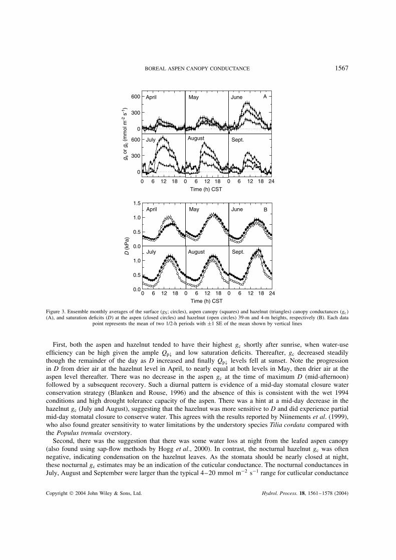
Figure 3. Ensemble monthly averages of the surface (gS; circles), aspen canopy (squares) and hazelnut (triangles) canopy conductances (gc(A), and saturation deficits (D at the aspen (closed circles) and hazelnut (open circles) 39-m and 4-m heights, respectively (B). Each data

point represents the mean of two 1/2-h periods with š1 SE of the mean shown by vertical lines

First, both the aspen and hazelnut tended to have their highest gc shortly after sunrise, when water-useefficiency can be high given the ample Qp# and low saturation deficits. Thereafter, gc decreased steadilythough the remainder of the day as D increased and finally Qp# levels fell at sunset. Note the progressionin D from drier air at the hazelnut level in April, to nearly equal at both levels in May, then drier air at theaspen level thereafter. There was no decrease in the aspen gc at the time of maximum D (mid-afternoon)followed by a subsequent recovery. Such a diurnal pattern is evidence of a mid-day stomatal closure waterconservation strategy (Blanken and Rouse, 1996) and the absence of this is consistent with the wet 1994conditions and high drought tolerance capacity of the aspen. There was a hint at a mid-day decrease in thehazelnut gc (July and August), suggesting that the hazelnut was more sensitive to D and did experience partialmid-day stomatal closure to conserve water. This agrees with the results reported by Niinements et al. (1999),who also found greater sensitivity to water limitations by the understory species Tilia cordata compared withthe Populus tremula overstory.

Second, there was the suggestion that there was some water loss at night from the leafed aspen canopy(also found using sap-flow methods by Hogg et al., 2000). In contrast, the nocturnal hazelnut gc was oftennegative, indicating condensation on the hazelnut leaves. As the stomata should be nearly closed at night,these nocturnal gc estimates may be an indication of the cuticular conductance. The nocturnal conductances inJuly, August and September were larger than the typical 4–20 mmol m2 s1 range for cutlicular conductance



(Jones, 1992), but these night-time calculations must be interpreted cautiously because E was near zero andnight-time eddy covariance measurements can behave erratically with low night-time turbulence, thereforepotentially underestimating night-time soil-water evaporation.

Controls on aspen and hazelnut canopy conductances

Whereas the general seasonal trends in gc were largely a function of al, the diurnal patterns were largely afunction of the ambient environmental conditions. It is well known that the stomatal conductance of almostall terrestrial plants responds to Qp#, CO2 concentration, water status, humidity, temperature, pollutants, leafphenology and nutrition (Jones, 1992). Forest species are especially sensitive at the diurnal scale to Qp# andhumidity, with the latter possibly a result of the high aerodynamic roughness of forests.

Table I shows several popular forms of the relationships between gc and several variables when the canopieswere dry and Qp# above the aspen exceeded 200 µmol m2 s1. Simple relationships between gc and Da orD0 were chosen on the basis of the likelihood of a strong response in forests well coupled to the surroundingatmosphere and follows the non-linear least-squares approach of Stewart (1988). These empirical relationshipsbetween gc and D are often criticized for their empiricism and lack of physical interpretation (i.e. physiologicalmechanisms) (Collatz et al., 1991). In response to these criticisms, advances have been made in a moreprocess-orientated relationship, relating gc to An, humidity and c

0 as Anh0/c0; we refer to the arrangement of

these variables as the Ball–Woodrow–Berry index (BWB; Ball et al., 1987). The BWB index is claimed tobe universal amongst C3, C4 or conifer species (parameterized by controlled leaf chamber measurements ofgc against Anh0/c

0 with linear regressions yielding slopes of 9, 4 and 6, for C3, C4 and conifers, respectively,and y-intercepts of 10 and 40 mmol m2 s1 for C3 and C4, respectively).

What follows is a discussion of the various relationships given in Table I and how these relationships mayor may not be used as useful predictors of gc. Of note, the least scatter (lowest mean SD) was observed whenthe aspen or hazelnut gc was plotted against An/(D0c

0. In general, An served as a good predictor for theaspen gc and the use of D0 instead of Da decreased the scatter for the hazelnut gc.

Saturation deficit control

The relationship between gS and the aspen and hazelnut gc to Qp# and humidity, with humidity expressedas a vapour pressure deficit at the leaf surface (D0, is shown in Figure 4. Relating conductance to D0 ratherthan Da decreased the amount of scatter in gS or gc –D plots, especially in the case of the hazelnut, whichwas less coupled to the air outside the leaf boundary layer than the aspen (Table I).

Owing to the compounding influence of light on the relationship between gc and D0, the data were groupedaccording to high Qp# (Qp# ½ 1400 µmol m2 s1, medium Qp# (800 < Qp# < 1400 µmol m2 s1 andlow Qp# (200 Qp# 800 µmol m2 s1 light. For both species and for the surface, there was a non-linear decrease in gc with D0 (described best by the non-linear curve fit gS or gc D gmax exp(-bD0 withthe relationships maintained as Qp# decreased. Similar non-linear responses have been observed for severalspecies (Oren et al., 1999), and this supports the conclusion that stomata respond to the transpiration rate itself,not humidity, as shown by Mott and Parkhurst (1991) and reiterated by Monteith (1995a), because this impliesthat E is constant and independent of D (however expressed) with all other variables held constant. Moreover,a non-linear response of gc to D suggests a constant ∂An/∂E and therefore a high water-use efficiency (Lloyd,1991). In the case of gc D a exp(-bD0, the maximum E occurred when D0 D 1/b or 1Ð89, 1Ð29 and 1Ð08 kPaat high, medium and low Qp#, respectively.

Carbon assimilation control

Determining the relationship between gc and the BWB index from canopy-scale measurements presumablydoes not require Fc measurements to be separated between aspen overstory and hazelnut understory becauseboth are C3 species, so the relationships should be the same (m D 9, b D 10 mmol m2 s1; Sellers et al.,1996). Only the soil respiration needs to be removed from Fc to obtain the forest An. Overstory and understory



Table I. Relationship between 1/2-hourly full-leaf (June 1–September 7, 1994) dry canopy, Qp# > 200 µmol m2s1 canopyconductance and variables known to affect gc, listed from least to highest scatter. Saturation deficits were expressed as molefractions. Parameters were determined from means calculated over 20 equally spaced bins. Data were excluded when the

n/total n was less than 5%

(a) Aspen

Functional relationship(gc in mmol m2 s1

a b r2 Mean standarddeviation (mmol m2 s1

Total n(1/2 h)

gc D aAn/(D0c0 C b 0Ð038 142Ð1 0Ð93 118Ð6 1717

gc D aAn/D0 C b 99Ð1 150Ð8 0Ð93 121Ð1 1729gc D aAn/Da C b 89Ð8 157Ð3 0Ð94 127Ð7 1730gc D aAnh0/c

0 C b 9Ð20 105Ð0 0Ð97 127Ð9 1735gc D aAnh0 C b 26556 101Ð5 0Ð98 128Ð1 1734gc D aAn/(Dac

a C b 0Ð032 155Ð7 0Ð94 128Ð9 1713gc D aAn C b 11372 133Ð0 0Ð92 139Ð0 1738gc D aAnha/c

a C b 2Ð57 129Ð4 0Ð96 144Ð8 1738gc D aD0 C b 11146 413Ð5 0Ð98 145Ð1 1758gc D a exp (bD0 438Ð2 38Ð8 0Ð98 145Ð1 1758gc D aAnha C b 6964 136Ð4 0Ð98 150Ð0 1734gc D aDa C b 10243 394Ð6 0Ð99 151Ð8 1774gc D a exp (bDa 414Ð6 36Ð4 0Ð98 151Ð8 1774

(b) Hazelnut

Functional relationship(gc in mmol m2 s1

a b r2 Mean standarddeviation (mmol m2 s1

Total n(1/2 h)

gc D aAn/(D0c0 C b 0Ð031 38Ð8 0Ð94 58Ð2 1427

gc D aAn/D0 C b 78Ð2 39Ð5 0Ð97 62Ð2 1474gc D aD0 C b 9695Ð1 204Ð6 0Ð84 65Ð7 1510gc D a exp (bD0 247Ð7 92Ð3 0Ð93 65Ð7 1510gc D aDa C b 9063Ð7 170Ð6 0Ð85 109Ð8 1617gc D a exp (bDa 193Ð4 59Ð8 0Ð89 109Ð8 1617gc D aAnh0/c

0 C b 1Ð30 105Ð4 0Ð11 112Ð8 1495gc D aAnh0 C b 4944Ð0 102Ð0 0Ð29 115Ð0 1539gc D aAnha/c

a C b 0Ð54 133Ð2 0Ð94 115Ð1 1597gc D aAn/(Dac

a C b 0Ð021 63Ð0 0Ð95 116Ð9 1561gc D aAn C b 5414Ð9 152Ð0 0Ð89 118Ð5 1598gc D aAn/Da C b 54Ð0 65Ð4 0Ð99 119Ð0 1563gc D aAnha C b 1699Ð3 136Ð7 0Ð76 121Ð9 1597

eddy-covariance measurements, however, facilitated the isolation of the aspen canopy An (i.e. Fc at the 4-mlevel subtracted from that at the 39-m level), but to determine the An of the hazelnut (CO2 respiration fromthe soil subtracted from Fc at the 4-m level), the soil respiration first had to be determined.

The daytime Rsoil was estimated from the biological relationship between soil temperature at the 2-cm depth (Ts and the night-time storage-corrected 4-m Fc (Fc(storage) D zc

a/t) and the systematicunderestimation of Fc at low wind speeds (Blanken et al., 1998). The relationship was best described bythe exponential function Rsoil D 0Ð4349 exp(0Ð2094 Ts, similar to that reported by Black et al. (1996). Thenet assimilation must be calculated when using the BWB index. As the focus here is not to model An, itwas estimated as a simple function of Qp# (Figure 5). In addition to serving as an effective empirical model,Figure 5 also reveals a well-defined relationship from which several salient physiological parameters weredetermined.



0

600

1200

15

30

g s o

r g c

(m

mol

m-2

s-1

)

0

300

600

mm

s-1

10

20

D0 (kPa)

0.0 0.5 1.0 1.5 2.0 2.5 3.00

150

300

0

5

10

Forest gs

Aspen gc

Hazelnut gc

Figure 4. Empirical relationships between the surface (gS or canopy (gc conductance and the 1/2-h saturation deficit at the bigleaf surface (D0 and for the full-leaf period when stratified by high (Qp# ½ 1400 µmol m2 s1; circles and solid line), medium(800 < Qp# < 1400 µmol m2 s1; squares and dashed line) and low Qp# (200 Qp# 800 µmol m2 s1; triangles and dotted line)incident photosynthetic photon flux density (Qp#. Mean values of gS and gc were calculated at binned 0Ð25 kPa intervals of D0. Non-linearcurve fits (lines) are of the form gS or gc D gcmax exp(bD0. Vertical lines are C1, š1 and 1 SD (high, medium and low Qp#, respectively)

Qp (µmol m-2 s-1)

0 500 1000 1500 2000

CO

2 A

ssim

ilatio

n (µ

mol

m-2

s-1

)

0

5

10

15

20

Figure 5. Relationship between net CO2 assimilation (An by the aspen (solid) and hazelnut (open) and incident photosynthetic photon fluxdensity (Qp# at the 39-m and 4-m heights. Mean values of An were calculated corresponding to a binned 1/2-h Qp# width of 100 (aspen)and 20 (hazelnut) µmol m2 s1. Solid lines represent rectangular hyperbolic curve fits An D ˛Qp#b/(˛Qp# C b R, where ˛, b and Rwere 0Ð0259, 31Ð2123 and 0Ð1646 (aspen), and 0Ð0786, 9Ð6638 and 0Ð9381 (hazelnut), respectively. Aspen and hazelnut r2 were 0Ð99and 0Ð88, respectively. Dashed line shows an extrapolation of the hazelnut Qp# to simulate overstory Qp# levels. The vertical lines are š1

SE of the mean



The An –Qp# relationship for both species was non-linear and best described by a rectangular hyperbolicfunction. The hazelnut had a higher quantum yield (slope at the origin) than the aspen (0Ð0786 and0Ð0259 mol mol1, hazelnut and aspen, respectively) and a lower photosynthetic capacity (An at Qp# D1800 µmol m2 s1 of 10Ð0 µmol m2 s1 compared with the aspen’s 18Ð8 µmol m2 s1, the formercharacteristic of shade-tolerant species (Salisbury and Ross, 1992). Dark respiration rates (D An whenQp# D 0) were higher for the hazelnut (0Ð94 µmol m2 s1 than the aspen (0Ð16 µmol m2 s1. Comparingthese results with an exhaustive review of An –Qp# relationships by Ruimy et al. (1995) shows that the non-linear relationships reported here are typical for forests. The boreal aspen quantum yield, photosyntheticcapacity and dark respiration rate were all lower than the 0Ð037 mol mol1, 21Ð39 µmol m2 s1 and3Ð34 µmol m2 s1, respectively, reported as means for several temperature deciduous forests. There were nounderstory species given for comparison.

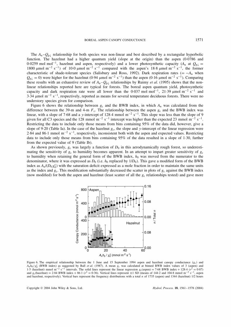
Figure 6 shows the relationship between gc and the BWB index, in which An was calculated from thedifference between the 39-m and 4-m Fc. The relationship between the aspen gc and the BWB index waslinear, with a slope of 7Ð68 and a y-intercept of 128Ð4 mmol m2 s1. This slope was less than the slope of 9given for all C3 species and the 128 mmol m2 s1 intercept was higher than the expected 23 mmol m2 s1.Restricting the data to include only those means from bins containing 95% of the data did, however, give aslope of 9Ð20 (Table Ia). In the case of the hazelnut gc, the slope and y-intercept of the linear regression were2Ð84 and 86Ð1 mmol m2 s1, respectively, inconsistent both with the aspen and expected values. Restrictingdata to include only those means from bins containing 95% of the data resulted in a slope of 1Ð30, furtherfrom the expected value of 9 (Table Ib).

As shown previously, gc was largely a function of D0 in this aerodynamically rough forest, so underesti-mating the sensitivity of gc to humidity becomes apparent. In an attempt to impart greater sensitivity of gc

to humidity when retaining the general form of the BWB index, h0 was moved from the numerator to thedenominator, where it was expressed as D0 (i.e. h0 replaced by 1/D0. This gave a modified form of the BWBindex as An/(D0c

0 with the saturation deficit expressed as a mole fraction in order to maintain the same unitsas the index and gc. This modification substantially decreased the scatter in plots of gc against the BWB index(now modified) for both the aspen and hazelnut (least scatter of all the gc relationships tested) and gave more

n / T

otal

n

0.00

0.08

0.16

Can

opy

Con

duct

ance

(m

mol

m-2

s-1

)

0

400

800

Anh0 / χ0c (mmol m-2 s-1)

0 20 40 600.00

0.08

0

200

400

Aspen

Hazelnut

Figure 6. The empirical relationship between the 1 June and 15 September 1994 aspen and hazelnut canopy conductance (gc andAnh0/c

0 (BWB index) as suggested by Ball et al. (1987). A mean gc was calculated at binned BWB index values of 3 (aspen) and1Ð5 (hazelnut) mmol m2 s1 intervals. The solid lines represent the linear regression gc(aspen) D 7Ð68 BWB index C 128Ð4 (r2 D 0Ð87)and gc(hazelnut) D 2Ð84 BWB index C 86Ð1 (r2 D 0Ð36). Vertical lines represent š1 SD (means of 144Ð2 and 104Ð8 mmol m2 s1, aspenand hazelnut, respectively). Vertical bars represent the frequency distributions with a total n of 1735 (aspen) and 1344 (hazelnut) 1/2 hours



consistent slopes for both species (35Ð0 and 31Ð4, aspen and hazelnut, respectively; Figure 7). Lloyd (1991)also obtained better results in predicting the gc of Macadamia integrifolia when h0 was replaced by 1/D0.

The rational for making this modification to the BWB index lies in the relationship between gc and humidity.The BWB index in its original form assumes that gc is a linear function of h0. Allowing leaf temperature(Tl to vary through a wide range may demonstrate the expected non-linear relationship, as leaf chambermeasurements are often operated within a narrow Tl range, where a non-linear curve may be approximatedby a straight line. Especially in forests where D0 plays a large role in gc, the non-linear response is demandedin gc calculations.

There is considerable debate as to whether plants actually respond to h0 at all, but are actually respondingto D0 (Aphalo and Jarvis, 1991). Further, h0 is a composite of both a humidity and temperature response(although in the aspen, T0 drives D0 and Tl may be required as a variable regulating gc, because gc sometimesresponds to Tl at constant D0 (Aphalo and Jarvis, 1993). Mott and Parkhurst (1991) further show that theapparent response of stomata to D0 is actually a response to the transpiration rate itself. This conclusion wassupported by Monteith (1995a), who shows that in 52 sets of measurements on 16 species, stomata respondedto the transpiration rate, not humidity. As stated by Monteith (1995a) ‘If the true response is to transpirationrate, however, predictions from these models must be flawed.’ (p. 357), where ‘models’ refers to predictinggc as an empirical function of D or h.

Predicting aspen conductance and transpiration

It still can be instructive, however, to calculate diurnal patterns of gc using the empirical relationships andparameters in order to offer validation of the functional relationships. Although this procedure does not useindependent data, it does indicate how reliably variations in the 1/2-hourly canopy conductance are simulated.Given the dominance of the aspen over the hazelnut gc in terms of gS and the desirability of single-layeredmodelling approaches, only the aspen gc was calculated from the empirical relationships. The parameters andrelationships determined over the entire full-leaf period from 1/2-h dry canopy, daytime measurements weretested against the 1/2-h measured aspen gc and E from 13 August to 18 1994. These days represent a range

n / T

otal

n

0.00

0.08

0.16

0

400

800

0 5 10 150.00

0.08

0.16

0

200

400

Aspen

Hazelnut

An / (D0 χ0c (mmol m-2 s-1)

Can

opy

Con

duct

ance

(m

mol

m-2

s-1

)

Figure 7. The empirical relationship between the 1 June and 15 September 1994 aspen and hazelnut canopy conductance (gc and a modifiedform of the BWB index, where h0 has been replaced by 1/D0 to improve the sensitivity of gc to humidity. A mean gc was calculated atbinned modified BWB index values at 0Ð75 (aspen) and 0Ð30 (hazelnut) mol m2 s1 intervals. The solid lines show linear regressions withslopes, y-intercepts and r2 of 35Ð0, 135Ð6 mmol m2 s1 and 0Ð91 (aspen) and 31Ð4, 40Ð4 mmol m2 s1 and 0Ð95 (hazelnut), respectively.The vertical lines show š1 SD (means of 152Ð1 and 76Ð1 mmol m2 s1, aspen and hazelnut, respectively). Vertical bars represent the

frequency distributions with a total n of 1717 (aspen) and 1278 (hazelnut) 1/2 h



in ambient conditions from clear to cloudy to overcast and a range in saturation deficits and air temperaturespeaking at the maximum observed Da over the entire year (15 August).

The aspen gc was first calculated as gc D a exp(bDa and then as gc D a exp(bD0, with a and b as afunction of Qp# in both cases. To move from the air outside to inside the leaf boundary layer, an iterativeprocedure was used. First, the aspen E was calculated using the Penman–Monteith equation with the initialgc D a exp(-kDa

E D sRa0 C acpDaga

s C 1 C ga/gc8

where H0 was estimated as H0 D Ra0 E, with Ra0 the available energy at the aspen big-leaf surface.To estimate Ra0, the 1/2-h surface Ra was plotted against the measured aspen Ra0, where Ra0 D E(aspen) CH(aspen). This yielded the linear relationship (not shown) Ra0 D 0Ð78Ra C 1Ð6 Wm2 (r2 D 0Ð99, n D 10 259),which was used to estimate Ra0 for the aspen canopy. Equations (2) through to (4) were then used to calculatetemperature and humidity at the leaf surface. The ‘new’ gc recalculated as gc D a exp(-kD0 was comparedwith the initial gc and if the absolute value of the difference was less than 1 mmol m2 s1, the calculationswere repeated until convergence was obtained.

The results of this calculation with gc D fD0, Qp# are shown in Figure 8. This is essentially theJarvis–Stewart approach to estimating gc using independent multiplicative functions (Stewart, 1988). Thediurnal course of the measured gc was well represented by the calculated gc, even responding to changes inD0 induced by cloudy periods. In general, the calculated gc tended to overestimate the measured gc, especiallywhen D0 was low, with a mean measured and calculated gc of 268 and 324 mmol m2 s1, respectively, overthe 6-day period. Using Da instead of D0 resulted in only a slight difference in the calculation of gc (mean gc

of 316 mmol m2 s1 and an average of three iterations were required to move from Da to D0. The closeagreement in the diurnal patterns and in gc calculated either with D0 or Da implies that the aspen gc waslargely a function of D and was closely coupled to the air in the forest surface layer. The calculated aspenE produced a similar diurnal pattern to the measured E, again tending to overestimate when D was low,stemming from the overestimation of gc. Over the 6-day period the mean calculated aspen E of 137Ð5 W m2

calculated with gc D fD0, Qp# was almost identical to the 138Ð2 W m2 calculated from gc D fDa, Qp#,and both agreed well with the measured mean E of 133 W m2.

g c (

mm

ol m

-2 s

-1)

0

200

400

600

August 1994 (CST)

λE (

W m

-2)

0

100

200

300

13 14 15 16 17 18

Figure 8. Measured (thin lines) and calculated (thick lines) daytime dry-canopy 1/2-h aspen canopy conductance (gc and transpiration (E)calculated using gc D a exp(bD0 and E using the Penman–Monteith equation. This essentially is a test of the Jarvis–Stewart approach

using two variables, D0 and light



The calculation of gc using the BWB index was performed identically to the procedure described above forgc D fD0, Qp# using parameters given in Table Ia. The diurnal plots of the measured and calculated gc withgc D f(BWB index) (Figure 9) show an underestimation of the early morning high and an overestimation ofthe late afternoon low gc (i.e. a lack of sensitivity to D0. This pattern was not unique to these six test days,but was characteristic of the entire full-leaf period. The mean gc, however, was not seriously affected, withthe calculated mean of 284 mmol m2 s1 slightly higher than the measured mean of 268 mmol m2 s1.Without iterating (mean of two iterations) and just using ambient relative humidity and CO2 mol fraction gavea mean gc of 278 mmol m2 s1. The resultant 6-day daytime mean aspen E from the BWB calculated gc

of 139 and 134 W m2 (with h and c at or above the leaf surface, respectively) still compared favourablywith the measured E of 133 W m2.

The seemingly simple modification of the BWB index by replacing h0 by 1/D0 altered the calculation ofthe aspen gc and E (Figure 10). The incorporation of the non-linear D0 response was apparent by allowinggc to obtain its early morning high and decrease more during the afternoon. The early morning gc wasoften overestimated, resulting in a daytime mean calculated gc of 298 mmol m2 s1, above the measuredmean of 268 mmol m2 s1. Not using D and c at the leaf surface resulted in a slightly higher mean gc of300 mmol m2 s1, further from the measured value (a mean of three iterations were required to obtain gc

from D0 and T0. The tendency to underestimate the mid-day gc resulted in an underestimation of the aspenE at these times when E was large giving slightly worse performance on the diurnal E compared withthat determined with the unmodified BWB. Compared with the other simulations, the six-day daytime meanE of 132 W m2 (131 W m2 without iteration) was, however, closest to the measured E of 133 W m2.The improvement made in the 1/2-hourly gc calculation worsened the 1/2-hourly E predictions (althoughhidden by daily means), because the improvements in gc were made at times when E was small and theunderestimation of gc near mid-day was made at times when E was large.

Regional controls

Several authors (e.g. McNaughton and Spriggs, 1989; McNaughton and Jarvis, 1991; Monteith, 1995b)have recognized the importance of the accommodation between transpiring vegetation and the CBL. Thisaccommodation is maintained by a positive feedback between gc and Da. Increasing gc decreases H anddecreases the height of the CBL (the height of the CBL, zi, can be approximated by the rate of change of

g c (

mm

ol m

-2 s

-1)

0

200

400

600

λE (

W m

-2 )

0

100

200

300

August 1994 (CST)

13 14 15 16 17 18

Figure 9. Measured (thin lines) and calculated (thick lines) daytime dry-canopy 1/2-h aspen canopy conductance (gc and transpiration (E)with gc calculated using gc D aAnh0/c

a C b and E using the Penman-Monteith equation



0

200

400

600

0

100

200

300

g c (

mm

ol m

-2 s

-1)

λE (

W m

-2 )

August 1994 (CST)

13 14 15 16 17 18

Figure 10. Measured (thin lines) and calculated (thick lines) daytime dry-canopy 1/2-h aspen canopy conductance (gc and transpiration(E) calculated using gc D aAn/(D0c

0 C b and the Penman–Monteith equation for E

zi with time from an initial early morning zi as dzi/dt D H C 0Ð07 E)/(acpziv), where v is the strengthof the inversion at the top of the CBL (McNaughton and Spriggs, 1989) and vigour of entrainment of warm,dry air from above the capping inversion. This in turn decreases the CBL saturation deficits (less volume ofair to be humidified) and, as shown in Figure 4, increases gc thus completing the positive feedback cycle. Ifthe initial response was a decrease in gc, H would increase, promoting growth of a drier, deeper CBL withincreasing saturation deficits and a decreasing gc; again positive feedback since the direction of the initial gc

response was maintained. This must not be confused with the larger-scale regional negative feedback betweenE and the saturation deficit in the CBL, where E becomes insensitive to the CBL saturation deficit when Erates are high (as discussed in McNaughton and Jarvis, 1991).

The similarity between the air inside and outside the aspen leaf boundary layer and the CBL has been shownthrough the gc analysis described previously. Figure 11A shows the seasonal progression of this similarityexpressed quantitatively with the McNaughton and Jarvis (1983) coefficient. The bare canopy of 0Ð09(1 SD š 0Ð15) and 0Ð08 (1 SD š 0Ð08) with and without snow, respectively, increased to 0Ð36 (1 SD š 0Ð18)with a leafed canopy, indicating that the surface E was less coupled to the CBL when the forest had leaves. As generally increases as surface roughness decreases, the implication was that the forest was aerodynamicallysmoother with leaves than without. This was confirmed by the daytime mean aerodynamic conductances of84Ð8 and 71Ð0 mm s1, without and with leaves, respectively, both slightly less than the 100–200 mm s1

range typical for forests (Oke, 1987), an indication of just how aerodynamically smooth the aspen forestwas. Hence, the increase in was the result of both an increase in gc and a decrease in ga. The decrease incoupling as al increased also concurs with the gc –D positive feedback effect described above. Increasing gc

(by adding more leaves) lessens the influence of D in the CBL on gc because the CBL is shallow with poorentrainment of dry, warm air above the inversion layer.

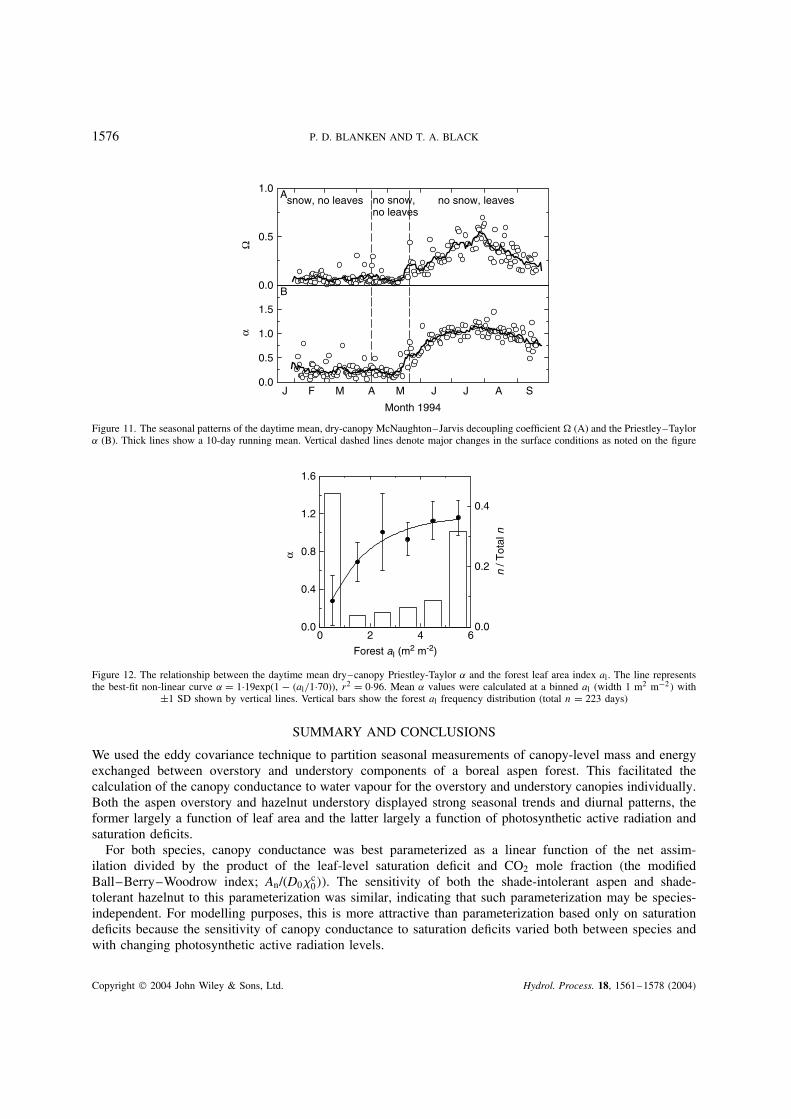
The Priestley–Taylor ˛ coefficient has been used to predict E from many types of surfaces (e.g.Spittlehouse, 1989). On a seasonal basis (Figure 11B) the mean daytime ˛ of 0Ð27 (1 SD š 0Ð24) and 0Ð30(1 SD š 0Ð29) with a bare canopy with and without snow, respectively, indicated that the surface E wasbelow the equilibrium rate owing to restrictions on the water supply. In contrast, the presence of a transpiringcanopy removed most of the restrictions on the water supply, increasing the daytime mean ˛ during thesnow-free, leafed period to 0Ð99 (1 SD š 0Ð28). During this period, E was limited largely by Ra, with onlyslight stomatal limitation on water supply. The relationship between ˛ and al was well defined by a non-linearrelationship (Figure 12) and shows the importance of gc via the linear relationship with al in regulating ˛.



α

0.0

0.5

1.0

Month 1994

Ω

0.0

0.5

1.0

1.5

snow, no leaves no snow,no leaves

no snow, leaves

J F M A M J J A S

B

A

Figure 11. The seasonal patterns of the daytime mean, dry-canopy McNaughton–Jarvis decoupling coefficient (A) and the Priestley–Taylor˛ (B). Thick lines show a 10-day running mean. Vertical dashed lines denote major changes in the surface conditions as noted on the figure

Forest aI (m2 m-2)

0 2 4 6

n / T

otal

n

0.0

0.2

0.4

α

0.0

0.4

0.8

1.2

1.6

Figure 12. The relationship between the daytime mean dry–canopy Priestley-Taylor ˛ and the forest leaf area index al . The line representsthe best-fit non-linear curve ˛ D 1Ð19exp(1 al/1Ð70)), r2 D 0Ð96. Mean ˛ values were calculated at a binned al (width 1 m2 m2 with

š1 SD shown by vertical lines. Vertical bars show the forest al frequency distribution (total n D 223 days)

SUMMARY AND CONCLUSIONS

We used the eddy covariance technique to partition seasonal measurements of canopy-level mass and energyexchanged between overstory and understory components of a boreal aspen forest. This facilitated thecalculation of the canopy conductance to water vapour for the overstory and understory canopies individually.Both the aspen overstory and hazelnut understory displayed strong seasonal trends and diurnal patterns, theformer largely a function of leaf area and the latter largely a function of photosynthetic active radiation andsaturation deficits.

For both species, canopy conductance was best parameterized as a linear function of the net assim-ilation divided by the product of the leaf-level saturation deficit and CO2 mole fraction (the modifiedBall–Berry–Woodrow index; An/(D0c

0. The sensitivity of both the shade-intolerant aspen and shade-tolerant hazelnut to this parameterization was similar, indicating that such parameterization may be species-independent. For modelling purposes, this is more attractive than parameterization based only on saturationdeficits because the sensitivity of canopy conductance to saturation deficits varied both between species andwith changing photosynthetic active radiation levels.



Working at the canopy level as opposed to the leaf level has the advantage of integrating the responses ofthousands of leaves. This work has shown that many of the physiological relationships determined from leaf-level research, often under controlled laboratory conditions, do apply at the canopy level. This is beneficialfor most land surface schemes because they operate at the canopy level. With the aspen canopy conductancerepresenting 70% of the forest conductance and the similarity in aspen and hazelnut physiological responsesto An/(D0c

0, we suggest that this forest be modelled as a single-layered aspen canopy using the modifiedBWB index with an effective leaf area index 43% larger than the actual aspen leaf area index. Evidence offeedback mechanisms between the surface and the convective boundary layer and their control on regionalevaporation rates were found and should be included in any modelling efforts made at this forest.

ACKNOWLEDGEMENTS

The Natural Sciences and Engineering Research Council of Canada (NSERC) in the form of a PostgraduateScholarship (P.D.B.) and a four-year collaborative Special Projects and Operating Grant (T.A.B.) providedfunding. A University of British Columbia Graduate Scholarship (P.D.B.) provided additional support. Thededicated efforts of many individuals made this research possible: Zoran Nesic, Paul Yang, Harold Neumann,Gerry den Hartog, Xuhie Lee, John Deary, Tom Hertzog, Monica Eberle, Mary Dahlman, Paula Pacholek,Murray Heap, Marian Breazu, Mary Yang, Jing Chen, Siguo Chen and Craig Russell. The constructivecomments and suggestions made by the three reviewers and Dr Norman Peters greatly improved the manuscriptand were greatly appreciated.

REFERENCES

Aphalo PJ, Jarvis PG. 1991. Do stomata respond to relative humidity? Plant, Cell and Environment 14: 127–132.Aphalo PJ, Jarvis PG. 1993. An analysis of Ball’s empirical model of stomatal conductance. Annals of Botany 72: 321–327.Baldocchi DD, Vogel CA, Hall B. 1997. Seasonal variation of energy and water vapor exchange rates above and below a boreal jack pine

forest canopy. Journal of Geophysical Research 102: 28 939–28 951.Ball JT, Woodrow IE, Berry JA. 1987. A model predicting stomatal conductance and its contribution to the control of photosynthesis under

different environmental conditions. In Progress in Photosynthesis Research, Biggins J (ed.). Martinus Nijhoff Publishers: Dordrecht;221–224.

Black TA, den Hartog G, Neumann HH, Blanken PD, Yang PC, Russell C, Nesic Z, Lee X, Chen SC, Staebler R, Novak MD. 1996. Annualcycles of water vapor and carbon dioxide fluxes in and above a boreal aspen forest. Global Change Biology 2: 219–229.

Black TA, Chen WJ, Barr AG, Arain MA, Chen Z, Nesic Z, Hogg EH, Neumann HH, Yang PC. 2000. Increased carbon sequestration by aboreal deciduous forest in years with a warm spring. Geophysical Research Letters 27: 1271–1274.

Blanken PD. 2002. Land/atmosphere interaction: canopy processes. In Encyclopedia of Atmospheric Sciences , Holton JR, Pyle J, Curry JA(eds). Academic Press: San Diego; 1121–1130.

Blanken PD, Rouse WR. 1996. Evidence of water conservation mechanisms in several subarctic wetland species. Journal of Applied Ecology33: 842–850.

Blanken PD, Black TA, Yang PC, Neumann HH, Staebler R, Nesic Z, den Hartog G, Novak MD, Lee X. 1997. The energy balance andcanopy conductance of a boreal aspen forest: Partitioning overstory and understory components. Journal of Geophysical Research 102:28 915–28 927.

Blanken PD, Black TA, Neumann HH, den Hartog G, Yang PC, Nesic Z, Staebler R, Chen W, Novak MD. 1998. Turbulent flux measure-ments above and below the overstory of a boreal aspen forest. Boundary-Layer Meteorology 89: 109–140.

Blanken PD, Black TA, Neumann HH, den Hartog G, Yang PC, Nesic Z, Lee X. 2001. The seasonal water and energy exchange above andwithin a boreal aspen forest. Journal of Hydrology 245: 118–136.

Bunce JA. 1985. Effect of boundary layer conductance on the response of stomata to humidity. Plant, Cell and Environment 8: 55–57.Collatz GJ, Ball JT, Grivet C, Berry JA. 1991. Physiological and environmental regulation of stomatal conductance, photosynthesis and

transpiration: a model that includes a laminar boundary layer. Agricultural and Forest Meteorology 54: 107–136.De Bruin HAR. 1983. A model for the Priestley–Taylor parameter ˛. Journal of Applied Meteorology 22: 572–578.Granier A, Loustau D, Breda N. 2000. A generic model of forest canopy conductance dependent on climate, soil water availability and leaf

area index. Annals of Forest Science 57: 755–765.Hall FG, Knapp DE, Huemmrich KF. 1997. Physically based classification and satellite mapping of biophysical characteristics in the southern

boreal forest. Journal of Geophysical Research 102: 29 627–29 580.Hogg EH, Saugier B, Pontailler JY, Black TA, Chen W, Hurdle PA, Wu A. 2000. Responses of trembling aspen and hazelnut to vapor

pressure deficit in a boreal deciduous forest. Tree Physiology 20: 725–734.Jones HG. 1992. Plants and Microclimate. Cambridge University Press: Cambridge; 428.



Kelliher FM, Lloyd J, Arenth A, Luhker B, Byers JN, McSeveny TM, Milukova I, Grigoriev S, Panfyorov M, Sogatchev A, Varlargin A,Ziegler W, Bauer G, Wong S-C, Schultze E-D. 1999. Carbon dioxide efflux density from the floor of a central Siberian Pine forest.Agricultural and Forest Meteorology 94: 217–232.

Lee XH, Black TA. 1993. Atmospheric turbulence within and above a Douglas fir stand. Part II: eddy fluxes of sensible heat and watervapor. Boundary-Layer Meteorology 64: 369–389.

Lloyd J. 1991. Modelling stomatal response to environment in Macadamia integrifolia. Australian Journal of Plant Physiology 18: 649–660.McNaughton KG, Jarvis PG. 1983. Predicting the effects of vegetation changes on transpiration and evaporation. In Water Deficits and Plant

Growth, Vol. VII, Kozlowski TT (ed.). Academic Press: New York; 1–47.McNaughton KG, Jarvis PG. 1991. Effects of spatial scale on stomatal control of transpiration. Agricultural and Forest Meteorology 54:

279–301.McNaughton KG, Spriggs TW. 1989. An evaluation of the Priestley and Taylor equation and the complementary relationship using results

from a mixed-layer model of the convective boundary layer. In Estimation of Areal Evapotranspiration, Black TA, Spittlehouse DL,Novak MD, Price DT (eds). IAHS Press: Wallingford; 89–104.

Monteith JL. 1995a. A reinterpretation of stomatal responses to humidity: theoretical paper. Plant, Cell and Environment 18: 357–364.Monteith JL. 1995b. Accommodation between transpiring vegetation and the convective boundary layer. Journal of Hydrology 116: 251–263.Monteith JL, Unsworth MH. 1990. Principles of Environmental Physics . Edward Arnold: London; 291.Mott KA, Parkhurst DF. 1991. Stomatal responses to humidity in air and helox. Plant, Cell and Environment 14: 509–515.Niinements U, Sober A, Kull O, Hartung W, Tenhunen D. 1999. Apparent controls on leaf conductance by soil water availability and via

light-acclimation of foliage structural and physiological properties in a mixed deciduous, temperate forests. International Journal of PlantSciences 160: 707–721.

Oke TR. 1987. Boundary Layer Climates , 2nd edn. Methuen: London; 435.Oren R, Sperry JS, Katul GG, Pataki DE, Ewers BE, Phillips N, Schafer KVR. 1999. Survey and synthesis of intra- and interspecific

variation in stomatal sensitivity to vapour pressure deficit. Plant, Cell and Environment 22: 1515–1526.Owen PR, Thompson WR. 1963. Heat transfer across rough surfaces. Journal of Fluid Mechanics 15: 321–334.Peterson EB, Peterson NM. 1992. Ecology, Management, and Use of Aspen and Balsam Poplar in the Prairie Provinces, Canada. Special

Report 1, Forestry Canada, Northwest Region, Northern Forestry Centre: Edmonton; 252.Priestley CHB, Taylor RJ. 1972. On the assessment of surface heat flux and evaporation using large-scale parameters. Monthly Weather

Review 100: 81–92.Ruimy A, Jarvis PG, Baldocchi DD, Saugier B. 1995. CO2 fluxes over plant canopies and solar radiation: a review. Advances in Ecological

Research 26: 1–68.Salisbury FB, Ross CW. 1992. Plant Physiology . Wadsworth: Belmont; 682.Sellers PJ, Hall FG, Baldocchi D, Cihlar J, Crill P, den Hartog J, Goodison B, Kelly RD, Lettenmeier D, Margolis H, Ranson J, Ryan M.

1994. BOREAS Experimental Plan, Chapters 1–3, Version 3Ð0. NASA: Greenbelt, MD.Sellers P, Hall F, Margolis H, Baldocchi D, den Hartog G, Cihlar J, Ryan MG, Goodison B, Crill P, Ranson KJ, Lettenmaier D, Wick-

land DE. 1995. The Boreal Ecosystem–Atmosphere Study (BOREAS): an overview and early results from the 1994 field year. Bulletinof the American Meteorology Society 76: 1549–1577.

Sellers PJ, Randall DA, Collatz GJ, Berry JA, Field CB, Dazlich DA, Zhang C, Collelo GD, Bounoua L. 1996. A revised land surfaceparameterization (SiB2) for atmospheric GCMs. Part I: model formulation. Journal of Climate 9: 676–705.

Schuepp PH, Leclerc MY, MacPerson JI, Desjardins RL. 1990. Footprint prediction of scalar fluxes from analytical solutions of the diffusionequation. Boundary-Layer Meteorology 50: 355–373.

Spittlehouse DL. 1989. Estimating evapotranspiration from land surfaces in British Columbia. In Estimation of Areal Evapotranspiration,Black TA, Spittlehouse DL, Novak MD, Price DT (eds). Publication No. 177, IAHS Press: Wallingford; 245–256.

Stewart JB. 1988. Modelling surface conductance of a pine forest. Agricultural and Forest Meteorology 43: 19–35.Verma SB. 1989. Aerodynamic resistances to transfers of heat, mass and momentum. In Estimation of Areal Evapotranspiration, Black TA,

Spittlehouse DL, Novak M, Price DT (eds). Publication No. 177, IAHS Press: Wallingford; 13–20.Wilson KB, Meyers TP. 2001. The spatial variability of energy and carbon dioxide fluxes at the floor of a deciduous forest. Boundary-Layer

Meteorology 98: 443–473.Wu A, Black A, Verseghy DL, Bailey WG. 2001. Comparison of two-layer and single-layer canopy models with Lagrangian and K-theory

approaches in modelling evaporation from forests. International Journal of Climatology 21: 1821–1839.


The canopy conductance of a boreal aspen forest, … Copies of my papers...The canopy conductance of...

Documents

Transcript of The canopy conductance of a boreal aspen forest, … Copies of my papers...The canopy conductance of...