The Bumpus house sparrow data: A reanalysis using ... · Evolutionary Ecology 1996, 10, 387-404 The...

Evolutionary Ecology 1996, 10, 387-404

The Bumpus house sparrow data: a reanalysis using structural equation models

B R U C E H. P U G E S E K 1 and A D R I A N T O M E R 2 1Southern Science Center, National Biological Service, 700 Cajundome Boulevard, Lafayette, LA 70506, USA 2Department of Psychology, Shippensburg University, Shippensburg, PA 17257, USA

Summary

We analysed the data of H.C. Bumpus on the survival of house sparrows (Passer domesticus) using structural equation modelling techniques. Using data on seven morphological variables measured by Bumpus, we tested and confirmed a three-factor model that characterized physical attributes for general size, leg size and head size. Although males were physically larger than females, we found no difference between males and females in the physical attributes as measured by the three factors. Survival increased significantly with increasing general size and was unrelated to leg size and head size. Wing length, independent of its relationship to the general size factor, was also significantly related to survival. Higher survival was found among birds with short wings. Males had a higher survival compared to females. Their higher survival was mediated, to a lesser extent indirectly, through greater size and, to a greater extent directly, through effects of unknown origin. We favour the use of structural equation modelling methods in studies of selection because of their ability to test and confirm or disconfirm hypotheses related to selection events.

Keywords: Bumpus; evolution; fitness; house sparrow; LISREL; natural selection; Passer domesticus; phenotypic selection; structural equation modelling; survival

Introduction

Bumpus (1899) studied domestic sparrows (Passer domesticus) subjected to the rigours of an ice and snow storm. Birds, immobilized by the storm, were collected and transported to the Brown University Anatomical Laboratory. Seventy-two sparrows, 51 males and 21 females, subsequently revived and 64, 36 males and 28 females, perished. Bumpus determined the sex of birds by plumage characteristics and concluded that there was a higher survival rate among males. He also measured nine phenotypic characteristics of the sparrows and concluded that seven of the nine characteristics provided evidence of 'selective elimination'. Compared to those that perished, survivors had a lower body weight, shorter total length and sternums, longer humerus, femur and tibio-tarsus lengths and wider skulls. The differences that he observed between live and dead birds in wing length and head-bill length were considered nominal and inconclusive.

A number of investigators have reanalysed Bumpus' data (e.g. Harris, 1911; Calhoun, 1947; Grant, 1972; Johnson et al., 1972; O'Donald, 1973) providing a useful means of illustrating and comparing ways to measure selection. Lande and Arnold (1983) used Bumpus' data to demonstrate methods for measuring the force of directional or stabilizing selection acting on phenotypic characteristics. They regressed survival on several phenotypic characteristics treated as independent variables. Multiple regression coefficients provided a function, called the selection gradient, for computing the shifts in multivariate phenotypic distribution resulting from the selection process. They interpreted each coefficient as the direct effect on fitness of a phenotypic characteristic. The effects of other correlated phenotypic characteristics are statistically adjusted away.

0269-7653 © 1996 Chapman & Hall

388 Pugesek and Tomer

Preliminary multivariate analysis of variance (MANOVA) by Lande and Arnold (1983) showed significant differences between the sexes in total length, weight, wing length and humerus and sternum length. Therefore, they performed separate multiple regressions on males and females. Results of multiple regression analyses indicated significant relationships between survival and weight in both sexes and between survival and total length in males only. Male survivors were lighter and shorter compared to those that died.

Several investigators argued that data from selection studies often violate the assumptions of the multiple regression model (Endler, 1986; Mitchell-Olds and Shaw, 1987; Crespi and Bookstein, 1989; Crespi, 1990). Under these circumstances, multiple regression coefficients are unstable (Gleser, 1992). Values of the coefficients can fluctuate due to measurement error and the presence or absence of other independent variables in the analysis (Crespi and Bookstein, 1989). Thus, multiple regression coefficients may not accurately depict relations between phenotypic characteristics and measures of fitness (Pugesek and Tomer, 1995).

Crespi and Bookstein (1989) (see also Crespi, 1990) advocated Wright's path analysis (1934) as an alternative to multiple regression for modelling selection. They conducted path analyses on the Bumpus data in which they created two unmeasured variables (i.e. factors). The first unmeasured variable, fitness, used survival as a single indicator. They derived the second unmeasured variable, a general factor corresponding to bird size, by a principal components analysis of the phenotypic characteristics. Using the size factor in a covariance analysis, they adjusted phenotypic characters for the difference in the mean values for live and dead birds. They regressed these size-adjusted 'shape coefficients' on survival. For each sex, they performed two analyses. One analysis used all nine phenotypic variables. The other analysis used the seven phenotypic variables remaining after excluding bird length and weight. The length of dead birds was likely to reflect an upwards bias due to post-mortem straightening of the spine. Bumpus' measurements of the weights of live birds probably reflected a downwards bias due to respiration and excretion between the time the birds revived and the time of weighing (Grant, 1972; Johnson et al., 1972).

In the nine-variable analysis, Crespi and Bookstein (1989) found significant paths to fitness only for the shape coefficients of weight in both sexes and also length in males. Survivors were lighter and, if males, also shorter. In the seven-variable analysis, a significant path to fitness was found only for the shape coefficient of wing length in males. They interpreted this to mean that birds with larger bodies relative to wing length were more likely to survive. No significant paths to fitness were found for females. While the covariance analysis used by Crespi and Bookstein (1989) provided selection coefficients or shape coefficients for characteristics, it did not provide a similar coefficient for the general size factor.

Crespi (1990) argued convincingly for the use of unmeasured variables, such as general body size, in selection studies. In this formulation of the selection model, selection may act directly on overall size and not only on the individual phenotypic characteristics that make up the size variable. Crespi (1990), with Bumpus' seven-variable data set on females, used a three-factor model to describe the physical characteristics of the birds. The first unmeasured variable was a general size factor derived from the first principal component of a factor analysis of the seven phenotypic characters. He derived the remaining two unmeasured variables from the residual correlation matrix remaining after extraction of the first factor. The second unmeasured variable, leg size, was a factor composed of two phenotypic characteristics, femur length and tarsus length. Crespi (1990) introduced this second factor because the residuals of the two components were highly correlated and the factor made substantive biological sense. He used the same rationale to formulate the third unmeasured variable, head size, a factor composed of head-bill length and head width. As in the previous analysis by Crespi and Bookstein (1989), the covariance analysis could not provide a selection coefficient for any of the factors.

Bumpus house sparrow data 389

The aforementioned analyses left several unanswered questions about the Bumpus data. First, can we interpret the first principal component as a general size factor? To try to answer this

question Crespi and Bookstein (1989) advocated the investigation of eigenvalues, residual correlations and the use of biological intuition as a basis for describing the pattern of relations among the phenotypic characteristics. An alternative, constituting in our view a more rigorous approach, involves the use of structural equation modelling (SEM) in a confirmatory factor analysis that can confirm or disconfirm the hypothesis of a size factor.

Second, what are the relationships between unmeasured variables based on phenotypic characteristics and fitness?

Third, are the general size, leg size and head size factors, different for males and females? In published path analyses, males and females were analysed separately, despite very small sample sizes. Do we need to treat males and females with separate analyses? Males were generally larger than females and had longer wings, etc. However, this does not imply that the composition of the factors differed between the sexes. Factors for males and females are the same unless the proportions of measured physical dimensions differ between the sexes.

Fourth, were sex-related survival differences mediated through the physical attributes measured by Bumpus? In particular, does the physically larger size of males explain why they had a higher survival rate than females?

In this paper, we addressed the above questions using SEM methods. In doing so, we pointed to several advantages of SEM over other methods of analysis. We preceded the analyses of the Bumpus data and their discussion with an explanatory section. This section provides, in a non- technical language, some of the basic concepts used in structural equation modelling.

Structural equation modelling (SEM)

General background

SEM encompasses an entire family of models known by many names: covariance structure analysis, confirmatory factor analysis, latent variable analysis and often as LISREL analysis. A number of books provide introductions to SEM (e.g. Hayduck, 1987; Bollen, 1989; Loehlin, 1994; Hair et al., 1995) and to computer software applications (e.g. Hayduck, 1987; Byrne, 1989, 1994). As one might expect from a method with so many variations in its application, researchers may question what constitutes structural equation modelling. Yet, we distinguish all structural equation models by two characteristics: (1) estimation of multiple and interrelated dependence relationships and (2) the ability to represent these relationships with latent variables.

Latent variables

Latent variables, sometimes called unmeasured variables or factors, are not measured directly, but are composites of directly measured variables called indicators. Latent variables are commonly represented by two or more indicators. A biological example of a latent variable is body size in a model that relates body size to survival. We can measure body size in different ways (length from head to tail, weight, etc.). These are measurements of observed variables that serve as indicators for the latent variable body size. By using a number of indicators for a latent variable, the researcher is proposing, in fact, a model. The model assumes that the latent variable or factor influences substantially the observed variables, which, therefore, can serve as indicators for the factor. This model constitutes a confirmatory factor analysis (CFA) model that we typically construct on the basis of a theory. As such, the model is in need of estimation and statistical testing. Figure 1 presents a CFA model for a case in which there are three latent variables, A, B and C, with two indicators each. Arrows leading from the latent variables to the indicators denote loadings that


Figure 1. A confirmatory factor analysis model in which there are three factors, with two indicators each. Latent variables (circles) and indicators (rectangles) are linked together by arrows. Single-headed arrows indicate the direction of relationships for model parameters - factor loadings and residual variances. Double-headed arrows indicate correlations among the factors.

represent the influence of the latent variable on the indicators. Our indicators for the latent variables are often imperfect. They are either imperfectly measured and/or they are affected by other variables not explicitly included in the model. We indicate this with the additional arrows representing error terms that lead to the indicators from the bottom up. These arrows denote the contribution of additional variance that is unrelated to the latent variable. Finally, we represent correlations between latent variables by double-headed arrows.

Confirmatory factor analysis can be contrasted with the older exploratory factor analysis (EFA). In the latter, researchers do not specify the relationships between latent variables and the indicator variables in advance as in CFA.

The measurement and the structural model in LISREL

Most SEM models include two parts, a measurement model and a structural model. The measurement model corresponds to the confirmatory factor analysis model mentioned above. It expresses how the researcher forms the latent variables. The structural model expresses the causal relationships between latent variables using a series of interdependent multiple regression equations. All relationships, in both the structural and the measurement model, are linear. The coefficients in the equations formulating the structural model are called path coefficients. In Fig. 2, letters A, B and C denote latent variables, a 1 and a 2 denote indicators for A, etc. Observe that variable A determines in part variable B which determines in part C. The direction of the arrows indicates the direction of relationships. Note that other variables (indicated by other arrows leading from above the latent variables) also affect B and C. These variables remain unspecified by the model.

Figure 2. A representative path diagram of a simple structural equation model with three latent variables, with two indicators each.


The function of theory

There are alternative possible connections between latent variables A, B and C and between them and the indicators. Therefore, the researcher should provide some justification for the model. This justification should be based on theory and previous studies that make the relationships presented in Fig. 2 plausible. For example, the researcher might know from previous research that a~ and a 2 are highly intercorrelated but weakly correlated with both the b and the c indicators. The researcher might also be willing to interpret an existing theory to suggest that A should influence B rather than vice versa, etc.

Statistical analyses in SEM

Researchers can estimate, test, and evaluate models such as the one presented in Figs 1 and 2 using computer programs such as LISREL (J6reskog and S6rbom, 1989). The Appendix provides additional explanation of model fitting and evaluation.

The Bumpus data and the present analyses

Because the process of dying could have strongly biased body length and body weight variables, we followed Crespi and Bookstein (1989) by excluding them from the present analyses. We performed logarithmic transformations on the remaining seven variables to meet the assumptions of normality (see also Lande and Arnold, 1983). We used sex and survival as additional variables in some models. In every case, the analysis used a matrix of correlations - tetrachoric, biserial or Pearson - according to the variables involved (dichotomous or continuous; see J6reskog and S6rbom, 1989). We produced matrices using PRELIS (J6reskog and S6rbom, 1986) and analysed using LISREL 7 (J6reskog and S6rbom, 1989) with the maximum likelihood method.

The measurement models - specification and estimation

One-factor measurement models. The measurement models for the Bumpus data specify the interrelationships between the phenotypic characteristics. We initially assumed that one factor, general size, underlies the relationships (correlations) between the seven variables (Fig. 3). In this simple model, we assumed the residuals of the indicators (phenotypic characteristics) to be uncorrelated. We estimated a stacked model (see the Appendix) simultaneously for males and females, assuming different constraints (see the Appendix) across the sexes. The formulation of these constraints allowed us to address the question of differences across sex: do male and female individuals in this population have the same shape? We evaluated three models to obtain a more precise formulation of this question.

(1) Model 1 - phenotypic characteristics have the same general pattern in males and females. In both sexes the same common faotors (in our initial model, just one common factor) explain the relationships among variables.

(2) Model 2 - as in model 1, both sexes have the same common factor. In addition, we constrained the loadings of the variables on the common factors (representing the extent to which the factors 'explain' the variables) to be equal in both sexes (see the Appendix).

(3) Model 3 - as in model 2, both sexes have the same common factor and loadings are constrained to be equal. In addition, we constrained the residual variances (accounting for the amount of variance unexplained in the morphological characteristics by general size) to be equal in both sexes.

The results of the estimation of these models (Table 1) suggested that even the most constrained model, model 3, which assumed the same factorial pattern, the same loadings and the sarne


Femur

Tarsus

Humeru_ s l~

'[ Wing ],1

Sternum ]4

Head I

Skull

Figure 3. The one-factor measurement model allowing for general size.

residuals across sexes, fit the data well. The fit of this model was not significantly poorer than the fit of the less-constrained model, model 2. The latter did not itself fit the data significantly poorer than the most relaxed model, model 1 (Table 1).

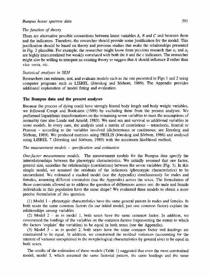
Three-factor measurement models. LISREL's modification indices (see the Appendix) indicated to us, however, that we could improve the one-factor model by freeing (see the Appendix) some covariances between residuals of the indicators. The modification indices for females were higher than 4 for two covariances. The covariance between head length and skull width and that between tarsus and femur also made sense biologically and morphologically. The existence of covariances between these residuals is also consistent with other analyses of the Bumpus data (Crespi, 1990). Figure 4 depicts a one-factor model allowing for the two covariances. These relationships may be the result of two additional factors. Each factor corresponds to one pair of variables and creates a covariance between these variables beyond and in addition to the covariance induced by general size. Following Crespi (1990), we called these factors head size and leg size (Fig. 5). In a simple

Table 1. Chi-squares and indices of fit for simultaneous confirmatory factor analyses in male and female house sparrows - three nested one-factor models

Model X 2 df p Ax2a Adf GFI b CFI c

1. Same factorial pattern (one factor) 43.59 28 0.030 0.953 0.975 2. Same factor loadings 50.39 35 0.045 6.80 7 0.942 0.975 3. Same factor loadings, same unique variances 62.08 42 0.024 11.69 7 0.931 0.968

a Successive differences between chi-squares starting from the most restrictive model. No difference attains significance at p --- 0.05. b Goodness-of-fit index (J6reskog and S6rbom, 1989). c Normed comparative fit index (Bentler, 1990).

Bumpus house sparrow data

x[ Femur ] ~ ~

~. Tarsus ]'

~ Humerus l ' - -

Sternum

W,no j'

~i Skull l~

393

Figure 4. A modified one-factor measurement model allowing for some covariances of residuals represented by double-headed arrows.

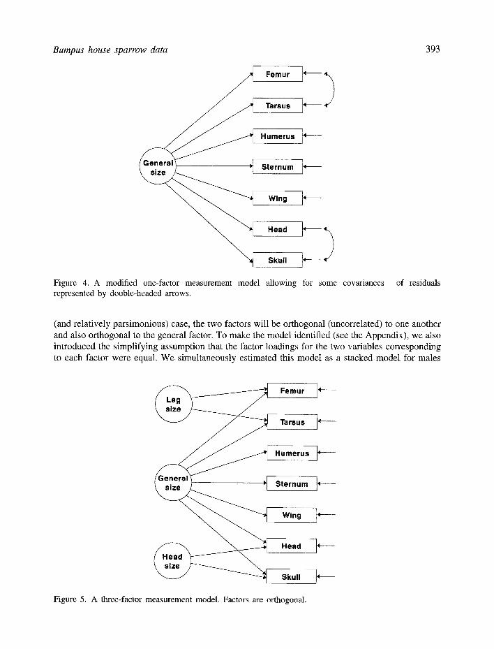
(and relatively parsimonious) case, the two factors will be orthogonal (uncorrelated) to one another and also orthogonal to the general factor. To make the model identified (see the Appendix), we also introduced the simplifying assumption that the factor loadings for the two variables corresponding to each factor were equal. We simultaneously estimated this model as a stacked model for males

Femur 4

Tarsus ]4 -

Humerus 4 -

Sternum ]4--

Wing ~ - -

Head ]~---

Skull ]~

Figure 5. A three-factor measurement model. Factors are orthogonal.


Table 2. Chi-squares and indices of fit for simultaneous confirmatory factor analyses in male and female house sparrows- three nested three-factor models

Model X z df p AX2a Adf GFI b CFI c

1. Same factorial pattern (three factors) 28.82 24 0.227 0.966 0.992 2. Same factor loadings 35.28 33 0.361 6.46 9 0.956 0.996 3. Same factor loadings, same unique variances 49.29 40 0.149 14.01 7 0.942 0.985

a Successive differences between chi-squares starting from the most restrictive model. No difference attains significance at p = 0.05. b Goodness-of-fit index (J6reskog and S6rbom, 1989). ° Normed comparative fit index (Bentler, 1990).

and females imposing sequentially the same constraints across sex that were used in the one-factor model.

The three-factor models fit the data very well, better in fact than the one-factor models (Table 2). Moreover, a comparison of the three nested models brought about a conclusion similar to the one based on one-factor models: the shape of the phenotypic characteristics was the same in females and males, even according to the most stringent definition of structural similarity imposed in model 3.

Some of the variables, such as humerus and femur, had high loadings of 0.9 or higher. Other variables such as sternum and skull were relatively poor indicators of the general size factors (Fig. 6). All loadings were highly significant (t-values > 6) (see the Appendix). The loadings corresponding to the other two factors, leg size and head size, were low but nevertheless significant (t-values > 4).

,274 Femur ~ .130

. Tarsus ~ .232

Humerus ~.095

(Gesn:eral ~ ,573 ~'J Sternum q.672

Wlng ~ .390

~ , 3 ~ ~ Head ''426

sku. I, 5 .8

Figure 6. Standardized loadings and residual variances for the most constrained three-factor model.

Bumpus house sparrow data 39:5

~I Femur

~I Tarsus

t' I Humerus

~'1 Sternum

-- *] Wing ~ / ~

,[ Hos----;

I~ I Skull

Figure 7. The survival model. Three latent variables are related to fitness which affects survival. Direct paths from morphological characteristics to fitness are fixed to 0.

The structural model - specification

The structural model related the latent variables underlying the morphological characteristics to fitness. Just one indicator, survival, measured fitness. We fixed the path from fitness to survival to 1 and the residual variance for survival was fixed to 0. We assumed that Bumpus measured survival without error (no dead birds being considered alive or vice versa) (Fig. 7).

We obtained a relatively parsimonious model by (1) allowing the paths from the three factors to fitness to be free and estimated and (2) fixing the direct paths from phenotypic characteristics (the indicator variables) to fitness to 0 (Fig. 7). However, some characteristics may have had a specific effect on survival independent of the relationships modelled through the path(s) from the latent variable(s). A model allowing all phenotypic characteristics to also affect survival is not, however, an identified model. We dealt with this problem by estimating first the model that allowed only the three factors to affect survival. Then, we freed more paths connecting phenotypic characteristics to fitness, if this could improve the fit. We used modification indices supplied by LISREL for this purpose.

The structural model - est imation

We estimated the survival model simultaneously as a stacked model (model 1 in Table 3) allowing only paths from the three factors to survival in males and females. Based on the results obtained fitting the measurement models, we assumed an invariant structure of morphological characteristics across sex. This means that, in both sexes, the same three factors explain relationships among the morphological characteristics. In addition, the loadings of the characteristics and the unique., variances or residuals are the same in males and females. Males obtained a relatively high modification index ( > 8) for the path from wing to survival. For this reason we released the constraint on this path. The new model 2 fit the data significantly better (Table 3). New modification indices for the paths to survival were low ( < 2) and therefore we decided not te release any other path coefficients.


Table 3. Chi-squares and indices of fit for simultaneous estimation in male and femal house sparrows of three survival models

Model number and description a X 2 df p GFI b CFI c

1. Three latent variables 62.72 48 0.075 0.925 0.977 2. Three latent variables, wing 52.37 46 0.241 0.945 0.990 3. Three latent variables and wing with equal paths 56.62 50 0.242 0.942 0.989 in males and females

a The description indicates the variables that are allowed to affect fitness. b Goodness-of-fit index (J6reskog and S/3rbom, 1989).

Normed comparative fit index (Bentler, 1990). Note: model 2 fits significantly better than model 1: X 2 (2) = 10.35, p < 0.01. Model 3 fits the data not significantly worse than model 2:×2 (4) = 4.25.

A further question of interest was whether or not the strength of the relationship between the latent variables (and, possibly, also phenotypic characteristics) and fitness was the same in males

and females. We addressed this question by setting the paths to fitness to be equal and by comparing the more-constrained model with the less-constrained model. The model obtained by constraining the paths to fitness appears as model 3 in Table 3. The difference in chi-squares between model 2 and model 3 was not significant. The parameters estimated in model 3 (Fig. 8) are likely to be more robust than the ones estimated in model 2.

The coefficient for the path f rom the general factor, general size, to fitness was significant. The negative sign for this coefficient indicates that a larger size is ' good for survival ' . The coefficients for the other two latent variables, leg size and head size, did not reach significance. In addition,

.13', I F . .u ,

. 3 , _ .

St.rnom

" ~ Wing

"425) t Head

"549) I Skull

Figure 8. Standardized path coefficients and residual variances for the survival model (model 3). All coefficients and variances are significant, t-values > 2, with the exception of the coefficients from leg size and head size to fitness.

Bumpus house sparrow data 39'7

wing also significantly affected fitness, but this coefficient is positive. A shorter wing length Jis related to a greater chance of survival.

A survival model with sex

We also specified a model including sex as an independent variable. In this model we allowed sex to affect general size (Fig. 9).

In addition to this, since there may be specific differences between the sexes, we modelled pathways from sex to all phenotypic characteristics, except skull. The path to skull was fixed to 0 to obtain identification of the model. We chose to fix the skull variable because there were few sex- related differences in skull measurements. The three factors could also affect survival. Estimation of such a model produced a chi-square of 47.44 with 16 degrees of freedom, goodness-of-fit index (GFI) = 0.936. An examination of the modification indices produced by LISREL showed the existence of a very large modification index for the path between wing and fitness ( > 25). We freed this path and obtained a new model with the following indicators of fit: X2(15) = 20.27, p = 0.162, GFI = 0.970, comparative fit index (CFI) = 0.994. The new model (Fig. 10) fit the

data significantly better: X2(]) = 27.17, p < 0.001. The new modification indices for the paths to fitness were all small ( < 2) and therefore we made no further modifications. The coefficients from the general size factor and from wing to fitness were significant (see Fig. 10). This agrees with the results obtained in the previous section. Males had a better chance of surviving. Sex was related significantly to two of the phenotypic characteristics, sternum and wing, which are bigger in males. The squared multiple correlation for fitness was R 2 = 0.345, substantially greater than 0.145 (for females) and 0.154 (for males) obtained by estimating models within sex. The improvement in the percentage of explained variance, together with an examination of the path coefficients in Fig. 10, suggests that sex played an important role in determining survival, independent of morphological characters.

¢

\

,x " ~ ~/ 1 Survival

Figure 9. A survival model with sex as an independent variable.


1. "~'145 I 21~ )k

///J~_ .umem. ~~~~ ~~¢o

-.164

Wing

Head

Skull

.848*

Figure 10. Standardized path coefficients for a survival model with sex. An asterisk denotes significance, t-value > 2. For model identification purposes, values of coefficients for general size to wing, and for coefficients of indicators of leg size and head size, were set to 1 in the unstandardized solution. For this reason, we did not calculate t-values for these coefficients.

Discussion

Summary of analyses Our main conclusions of the structural equation modelling analyses are as follows.

(1) The seven phenotypic characteristics analysed here have three underlying unmeasured variables or factors and the relationships between the factors and the characteristics are the same in males and in females.

(2) A general size factor affects survival, reflecting an advantage for larger size. (3) A short wing length is conducive to better survival. (4) Relationships between these characteristics and survival are not significantly different in

males versus females. (5) The sex of the bird affects survival indirectly through conveyance of larger size to males and

directly giving an advantage to males versus females that is independent of morphological

characteristics.

These results are consistent with other results presented in the literature (e.g. Crespi and Bookstein, 1989; Crespi, 1990) but they also add to them. We asked and answered, for the first time, the question of structural similarity in females versus males. The present analysis also continued the line of thought presented by Crespi (1990) and by Crespi and Bookstein (1989) who introduced latent variables in their analyses. In addition to the existence of a relationship between wing and survival that Crespi and Bookstein (1989) had already established, our analyses confirmed the existence of a relationship between a general size factor and survival. Finally, we


partitioned the relationship between sex and survival into direct and indirect components mediated through body size.

Methodological comments

Structural equation modelling (SEM), as illustrated by the LISREL models presented and estimated here, can be a very versatile method in the measurement of selection. Our study exposed some of the applications of SEM and the LISREL model in the examination of structures of phenotypic characteristics and in the comparison of structures in different populations such as males and females. In addition, we applied SEM to examine the relationships of phenotypic characteristics to fitness by formulating plausible models, by estimating these models and by assessing their fit to the data. We also showed how the models could be modified according to various indicators, such as modification indices.

We advocate several caveats concerning our analysis. First, although an exploratory use of SEM and of LISREL or equivalent models would be considered legitimate by many methodologists and statisticians (e.g. MacCallum, 1986; Anderson and Gerbing, 1988; J6reskog and S6rbom, 1989; S6rbom, 1989; Bentler, 1992), it is important to distinguish exploratory use from the purely confirmatory use of SEM. In an exploratory use of SEM there is a risk of capitalizing on chance that requires us to see the results (the acceptance of one model over another) as tentative and in need of further confirmation. We should make this confirmation on the basis of additional data (e.g. Raykov et al., 1991). Our use of SEM was, in part, exploratory. We attained our three-factor measurement model only after examining the modification indices obtained for the one-factor measurement model. Similarly, in the survival model we freed the path from wing to fitness only after examining the modification index for this path. The survival model that we estimated and found to fit the data well should therefore be considered as a tentative model in need of further exploration and confirmation.

Second, while we believe the models considered here are plausible and fit the data well, it is always possible that there are other variables and/or causal assumptions that may generate models as 'successful' as the one considered here (e.g. Breckler, 1990) and these models may provide alternative interpretations.

Third, we estimate models on the basis of statistical assumption. One assumption in the use of the maximum likelihood method of estimation is multivariate normality of the variables included in the model. While much more relaxed assumptions can replace this distributional assumption, typically this requires very large sample sizes (Browne, 1984).

Sample size results in a fourth limitation. We estimate and compare models based, in part, on a statistic that is distributed asymptotically as a chi-square variable under the assumption of multivariate normality. Samples have to be large enough to use the statistic for tests of overall fit reliably, as well as to avoid non-convergence of the iterative procedure used for the maximum likelihood solution. There is uncertainty regarding the 'minimum sample size'. Boomsma (1985) suggested sample sizes of at least 100. Hayduck (1987) suggested samples of at least 50. A researcher planning to use the techniques and the type of models presented here should ideally collect data from a sample of 200 or more to avoid problems of convergence and/or validity of the chi-squares (Boomsma, 1982).

Finally some authors, albeit a minority (e.g. Bookstein, 1986; Freedman, 1991), oppose any use of LISREL or equivalent programs for structural equation models in areas in which the theory is still rudimentary and/or imprecise. Notwithstanding these limitations, we believe that, used judiciously, SEM may be a powerful tool in the measurement of selection and in advancing the formulation of theoretical models of selection.


Acknowledgements

We wish to thank Ziad Malaeb and Sijan Sapkota for critical reviews of this manuscript. Research was supported by NIA grant (T32-AG00110-03), the US Fish and Wildlife Service and the National Biological Survey. The mention of trade names of commercial products in this paper does not constitute endorsement or recommendation for use by the National Biological Service, US Department of Interior.

References

Anderson, J.G. and Gerbing, D.W. (1988) Structural equation modeling in practice: a review and recommended two-step approach. Psychol. Bull. 103, 411-23.

Anderson, J.G. and Gerbing, D.W. (1992) Assumptions and comparative strengths of the two-step approach. Sociol. Methods Res. 20, 321-33.

Bentler, P.M. (1990) Comparative fit indexes in structural models. Psychol. Bull. 107, 238-46. Bentler, P.M. (1992) EQS: A Structural Equation Program Manual. BMDP Statistical Software Inc., Los

Angeles, CA. Bentler, P.M. and Bonett, D.G. (1980) Significance tests and goodness of fit in the analysis of covariance

structures. Psychol. Bull. 88, 588-606. Bollen, K.A. (1989) Structural Equations with Latent Variables. Wiley, New York. Bookstein, F.L. (1986) The elements of latent variable models: a cautionary lecture. In Advances in

Developmental Psychology (M.E. Lamb, A.L. Brown and B. Rogoff, eds), pp. 203-30. Erlbaum, Hillsdale, NJ.

Boomsma, A. (1982) The robustness of LISREL against small sample size in factor analysis models. In Systems Under Indirect Observation: Part 1 (K. J6reskog and H. Wold, eds), pp. 149-73. North Holland, Amsterdam.

Boomsma, A. (1985) Nonconvergence, improper solutions, and starting values in LISREL maximum likelihood estimation. Psychometrika 50, 229-42.

Breckler, S.J. (1990) Application of covariance structure modeling in psychology: cause for concern? Psychol. Bull. 107, 260-73.

Browne, M.W. (1984) Asymptotically distribution-free methods for the analysis of covariance structures. Br. J. Math. Stat. Psychol. 37, 62-83.

Bumpus, H.C. (1899) The elimination of the unfit as illustrated by the introduced sparrow, Passer domesticus. Biol. Lect. Woods Hole Mar. Biol. Sta. 6, 20%26.

Byrne, B.M. (1989) A Primer of LISREL: Basic Applications and Programming for Confirmatory Factor Analytic Models. Springer Verlag, New York.

Byrne, B.M. (1994) Structural Equation Modeling with EQS and EQS/Windows. Sage Publications, Thousand Oaks, CA.

Calhoun, J.B. (1947) The role of temperature and natural selection in relation to the variations in the size of the English sparrow in the United States. Am. Nat. 81, 203-28.

Carmines, E. and McIver, J. (1981) Analyzing models with unobserved variables: analysis of covariance structures. In Social Measurement: Current Issues (G. Bohrnstedt and E. Borgatta, eds), pp. 65-115. Sage, Beverly Hills, CA.

Crespi, B.J. (1990) Measuring the effect of natural selection on phenotypic interaction systems. Am. Nat. 135, 32-47.

Crespi, B.J. and Bookstein, F.L. (1989) A path-analytic model for the measurement of selection on morphology. Evolution 43, 18-28.

Endler, J.A. (1986) Natural Selection in the Wild. Princeton University Press, Princeton, NJ. Freedman, D.A. (1991) Statistical models and shoe leather. Sociol. Method. 21, 291-313. Gleser, L.J. (1992) The importance of assessing measurement reliability in multivariate regression. J. Am.

Stat. Assoc. 87, 696-707. Grant, P.R. (1972) Centripetal selection and the house sparrow. Syst. Zool. 21, 23-30.


Hair, J.F., Anderson, R.E., Tatham, R.L. and Black, W.C. (1995) Multivariate Data Analysis. Prentice Hall, Englewood Hills, NJ.

Harris, J.A. (1911) A neglected paper on natural selection in the English sparrow. Am. Nat. 45, 314-18. Hayduk, L.A. (1987) Structural Equation Modeling with LISREL. The Johns Hopkins University Press,

Baltimore, MD. Johnson, R.K., Niles, D.M. and Rohwer, S.A. (1972) Hermon Bumpus and natural selection in the house

sparrow Passer domesticus. Evolution 26, 22-31. J6reskog, K.G. and S6rbom, D. (1986) PRELIS: A Preprocessor for LISREL. Scientific Software Inc.,

Mooresville, IN. J6reskog, K.G. and S6rbom, D. (1989) LISREL 7: A Guide to the Program and its Application. SPSS Inc.,

Chicago, IL. Lande, R. and Arnold, S.J. (1983) The measurement of selection on correlated characters. Evolution 37,

1210-26. Loehlin, J.C. (1994) Latent Variable Models. Lawrence Erlbaum Associates, Hillsdale, NJ. MacCallum, R. (1986) Specification searches in covariance structure modeling. Psychol. Bull. 100,

t07-20. Mitchell-Olds, T. and Shaw, R.G. (1987) Regression analysis of natural selection: statistical inference and

biological interpretation. Evolution 41, 1149-61. Mulaic, S.A., James, L.R., Van Alstine, J., Bennett, N., Lind, S. and Stilwell, C.D. (1989) Evaluation of

goodness-of-fit indices for structural equation models. PsychoL Bull. 105, 430-45. O'Donald, P. (1973) A further analysis of Bumpus' data: the intensity of natural selection. Evolution 27,

398-404. Pugesek, B.H. and Tomer, A. (1995) Determination of selection gradients using multiple regression versus

structural equation models (SEM). Biomet. J. 37, 449-62. Raykov, T., Tomer, A. and Nesselroade, J.R. (1991) Reporting structural equation modeling results in

psychology and aging: some proposed guidelines. Psychol. Aging 6, 499-503. Saris, W.E., Satorra, A. and S6rbom, D. (1987) The detection and correction of specification errors in

structural equation models. In Sociological Methodology 1987 (C.C. Clogg, ed.), pp. 105-30. American Sociological Association, Washington, DC.

S6rbom, D. (1989) Model modification. Psychometrika 54, 371-85. Steiger, J.H., Shapiro, A. and Browne, M.W. (1985) On the multivariate asymptotic distribution of sequential

chi-square statistics. Psychometrika 50, 253-64. Wright, S. (1934) The method of path coefficients. Ann. Math. Stat. 5, 161-215.

Appendix Data analysis in SEM

Data are collected about the indicators and used to evaluate the model. Input for the statistical analysis is the variance-covariance matrix or the correlation matrix. The statistical analysis has two main functions. One function is to estimate the free parameters (path coefficients, loadings and error terms) of the model. This function is analogous to the estimation of regression coefficients in a multiple regression analysis. However, coefficients are frequently derived using the maximum likelihood method of estimation (rather than the least squares that is commonly used in multiple regression). The researcher can fix some of the parameters of the model while formulating the model. For example, there is no arrow leading from A to C in Fig. 2, indicating that the path coefficient for this relationship was fixed to zero. Other parameters may be fixed in order to define a scale for the latent variables. The researcher can accomplish this by fixing to unity one loading per latent variable. The fixed parameters are not estimated, but rather assumed to be true as part of the model.

The second function of the statistical analysis is to determine how well the model fits the data. The researcher can use a chi-square statistic to determine that the likelihood of obtaining tile


data, given that the model is true, is not too low. If the likelihood is high enough, the researcher will not reject the hypothesis of 'good fit'. However, there are problems with using this test with small or large samples. We recommend instead using goodness-of-fit (GOF) indices. We discuss GOF indices further in the next section.

As previously explained, a complete model includes a measurement model and a structural model. Anderson and Gerbing (1988, 1992) advocated a two-step approach starting with the measurement model. If the measurement model fits the data well, indicating the satisfactory measurement of the latent variables, the researcher may proceed to fit the structural model.

What allows the investigator to evaluate model fit? In a regression equation, variances and covariances will determine the regression coefficients and vice versa. However, no test of the 'regression model' is possible. In a typical SEM application, constraints imposed by the researcher on the relationship between variables by fixing parameters make such a testing possible. The reason for this is that a model that we constrain 'enough' (i.e. is overidentified) has more variances and covariances than there are parameters to be estimated. For example, we have an overidentified model in Fig. 2. In this model there are six observed variables that provide 21 variances and covariances. It is possible to show that we need to estimate only 14 parameters (Fig. 11). The basis for testing this model or, indeed, any overidentified model, is the following. A model, including the estimated parameters, implies that the variances-covariances in the population have certain values. We can compare the model-implied variance-covariance matrix to its counterpart obtained from the data using the chi-square test mentioned earlier. In addition, we use the ratio xZ/df to evaluate the degree of fit: values of 2 or less are considered to indicate good fit (Carmines and McIver, 1981). Another method of evaluation is based on indices that quantify the distance between the obtained and the implied matrix. Examples of such indices are the goodness-of-fit index or GFI (J6reskog and S6rbom, 1989) and the normed comparative fit index or CFI (Bentler and Bonett, 1980; Bentler, 1990, 1992).

Indices of fit provide continuous values ranging typically from 0 to 1. Indices of magnitude of above 0.8, preferably 0.9, are considered to indicate a reasonably good fit.

While indices of fit deal with the overall fit of the model, the researcher is also interested in the estimates of particular parameters, such as path coefficients. For example, in the model presented in Fig. 1, of particular interest are the path coefficients from A to B and from B to C. Typically, we divide the estimated values for these coefficients by estimated standard errors to generate t-values. We use t-values to determine the precision of the estimated value as well as its statistical significance (J6reskog and S6rbom, 1989).

Identification It is also possible that the number of parameters left free for estimation is so large (in relation to the information available) that no unique identification is possible. A simple example is an equation

1 * 1 -k

Figure 11. Free parameters in the structural equation model from Fig. 1 are represented by asterisks on the paths (for path coefficients) or in the tails (for additional variances). Note that one free parameter, the variance of A, is not explicitly represented in the figure.


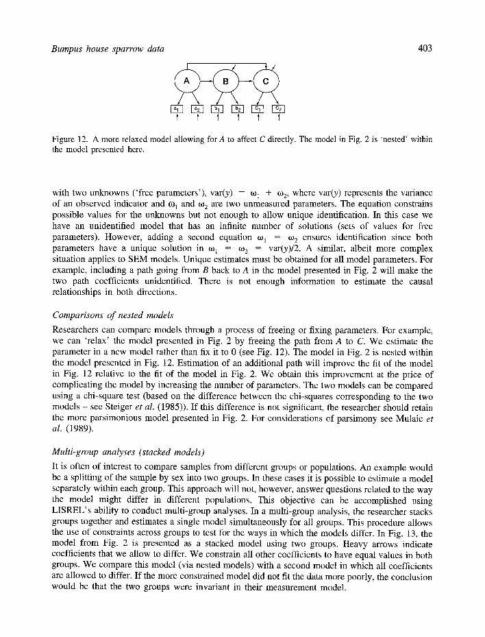
Figure 12. A more relaxed model allowing for A to affect C directly. The model in Fig. 2 is 'nested' within the model presented here.

with two unknowns ('free parameters'), var(y) = ~01 + t%, where var(y) represents the variance of an observed indicator and co 1 and to 2 are two unmeasured parameters. The equation constrains possible values for the unknowns but not enough to allow unique identification. In this case we have an unidentified model that has an infinite number of solutions (sets of values for free parameters). However, adding a second equation o~ 1 = o~ 2 ensures identification since both parameters have a unique solution in o~ l = 1.o 2 = var(y)/2. A similar, albeit more complex situation applies to SEM models. Unique estimates must be obtained for all model parameters. For example, including a path going from B back to A in the model presented in Fig. 2 will make the two path coefficients unidentified. There is not enough information to estimate the causal relationships in both directions.

Comparisons of nested models

Researchers can compare models through a process of freeing or fixing parameters. For example, we can 'relax' the model presented in Fig. 2 by freeing the path from A to C. We estimate the parameter in a new model rather than fix it to 0 (see Fig. 12). The model in Fig. 2 is nested within the model presented in Fig. 12. Estimation of an additional path will improve the fit of the model in Fig. 12 relative to the fit of the model in Fig. 2. We obtain this improvement at the price of complicating the model by increasing the number of parameters. The two models can be compared using a chi-square test (based on the difference between the chi-squares corresponding to the two models - see Steiger et al. (1985)). If this difference is not significant, the researcher should retain the more parsimonious model presented in Fig. 2. For considerations of parsimony see Mulaic et al. (1989).

Multi-group analyses (stacked models)

It is often of interest to compare samples from different groups or populations. An example would be a splitting of the sample by sex into two groups. In these cases it is possible to estimate a model separately within each group. This approach will not, however, answer questions related to the way the model might differ in different populations. This objective can be accomplished using LISREL's ability to conduct multi-group analyses. In a multi-group analysis, the researcher stacks groups together and estimates a single model simultaneously for all groups. This procedure allows the use of constraints across groups to test for the ways in which the models differ. In Fig. 13, the model from Fig. 2 is presented as a stacked model using two groups. Heavy arrows indicate coefficients that we allow to differ. We constrain all other coefficients to have equal values in both groups. We compare this model (via nested models) with a second model in which all coefficients are allowed to differ. If the more constrained model did not fit the data more poorly, the conclusion would be that the two groups were invariant in their measurement model.


Males ~/

t ! T T l T ~ma,os ~

T T T l l Y Figure 13. A stacked model for comparing two groups, males and females. Constraints imposed on the models allow for a statistical test of the similarity of the measurement models of the two groups.

Respecification and modification indices

Ideally, the user of SEM has a strong theory on which they can base the models. Models are more typically tentative and entertained as crude approximations. The researcher can use SEM to estimate and to evaluate these models and, on the basis of various indicators, propose a respecification of the model (e.g. Saris et al., 1987). Estimation proceeds on the new respecified models using the same set of data. The researcher can use modification indices provided by LISREL (J6reskog and S6rbom, 1989; S6rbom, 1989) to guide model respecification. A large ( > 4) modification index for a fixed parameter of the model indicates that releasing the parameter to be freely estimated will significantly improve the model.

The Bumpus house sparrow data: A reanalysis using ... · Evolutionary Ecology 1996, 10, 387-404 The...

Documents

Transcript of The Bumpus house sparrow data: A reanalysis using ... · Evolutionary Ecology 1996, 10, 387-404 The...