The Budget Deficit 357

ness investment caused by the combination of the Economic Recoveryand Tax Act of 1981 and the reduced rate of inflation. The tight moneypolicy is also seen as a cause of the dollar's rise in this period. But theauthors conclude that although expanding budget deficits in this period"may also have raised the level of U.S. real interest rates and helped tostrengthen the dollar. . . the extent of upward pressure on real interestrates and on the dollar through this channel is uncertain, and numerousstudies have failed to uncover significant effects" (p. 105).

The report's authors also note that after 1982 the differential betweenU.S. three-month real interest rates and a trade-weighted average ofthree-month real interest rates in six other indusflial countries (calcu-lated using OECD inflation forecasts) narrows to zero and is occasionallynegative. They conclude from this that "other factors have continued topush up the demand for dollar assets" and suggest that the dollar'sstrength since 1982 has been due to "the combination of increased after-tax profitability of U.S. corporations, demonstrated strength of the U.S.recovery, reversal of international lending outflow from U.S. banks,and generally more favorable longer run prospects for the U.S. econ-omy. . . ."(pp. 105—6).

Another commonly expressed opinion is that the rise in the dollarsince the summer of 1980 reflected growing confidence in the UnitedStates as a "safe haven" for investments by foreigners who believed thatthe election of Ronald Reagan would make their assets safer in theUnited States than elsewhere in the world. There is also the view, identi-fied most strongly with Ronald McKinnon (e.g., 1984), that the strongdollar does not reflect any "real" phenomena (budget deficits, increasedprofitability, alternative tax rules) but is solely an indication that mone-tary policy in the United States is too tight.

At a more fundamental level, any role for the budget deficit in explain-ing the rise of the dollar must be rejected by those economists who be-lieve that deficits do not raise real interest rates because they induce anequal offsetting rise in private saving (e.g., Barro 1974). Evans (1986) ex-tended the procedure of Plosser (1982) to study the relation between un-expected changes in budget deficits and the dollar and concluded thedollar exchange rate is not affected by changes in the budget deficit. Ireturn below to the deficiencies of this type of analysis.

Although there may be some element of truth in each of the alternativeexplanations of the dollar's rise, my own judgment is that they are not asimportant as the increase in expected structural budget deficits and theshift to a less inflationary monetary strategy. This is supported by theeconometric evidence presented in sections 4 through 6. The estimated

358' FELDSTEIN

effects of the expected deficits and of the rate of growth of the moneysupply are economically important and statistically significant. In con-trast, the increase in profitability induced by the tax changes in the firsthalf of the 1980s did not have a significant effect on the exchange rate inthe equations presented below. The strong statistical evidence of a linkbetween the expected structural budget deficits and the value of the dol-lar is direct evidence against the Barro hypothesis that budget deficitshave no real impact. The implied impact of the expected budget defi-cits also contradicts the McKinnon hypothesis that the rise of the dollarwas due only to a tight monetary policy.

Before I turn to that econometric evidence, I think it will be useful toconsider some further reasons for rejecting the arguments of those whoclaim that neither increased real interest rates nor budget deficits wasresponsible for the dollar's rise.

The evidence presented in the 1985 Economic Report of the President (andelsewhere) that there is no longer a difference between the three-monthreal interest rate in the United States and in other industrial countries isessentially irrelevant since the theory implies that the equilibrium rela-tion between the exchange rate and the difference in long-term real ratesis much larger than the relation with the difference in short-term realrates. It is easy to see why this is true. Consider the situation in whichthe U.S. three-month real rate is four percentage points above the three-month rate on foreign securities but there is no interest differential forintervals beginning after three months. Thus the six-month interest ratesdiffer by only two percentage points, the one-year rates differ by one per-centage point, and so on. The value of the dollar can be one percentagepoint above its equilibrium value since the interest rate differential isenough to compensate for a one percent decline in the dollar, regardlessof whether this happens in three months, six months, a year, or longer.But with the differential in real rates concentrated only in the three-month maturity, any greater overvaluation of the dollar would imply anexpected future decline not compensated by the difference in interestrates.

In contrast, consider the situation in which the real interest rate on theU.S. 10-year bond is 4 percentage points above the real yield on foreign10-year bonds with no interest differential for intervals after ten years.Then the real value of the dollar can fall by 4 percent a year for ten yearsand still leave an investor indifferent between having purchased dollarbonds and foreign bonds. This implies that a 4 percent real interest dif-ferential on 10-year bonds can support a 48 percent initial overvaluationof the dollar.

The Budget Deficit 359

It is noteworthy therefore that, although the three-month real yield dif-ferential reached zero by the end of 1982 and hovered around that levelthereafter, the long-term real interest differential at the end of 1983 wasin the range of two to four percentage points, depending on the methodof forecasting future inflation.4 The observed real interest differentialwas therefore quite consistent with the observed rise in the dollar's realvalue. I will return later to the more formal evidence on the link betweenthe dollar and the real interest differential.

While the change in U.S. monetary policy after October 1979 may havereduced the inflation risk in U.S. fixed-income securities, the notion thatthe dollar rose in the 1980s because the United States capital market is apolitical safe haven for foreign funds seems doubtful. Although theUnited States does offer a politically safe environment, it is hard to see arise in U.S. political stability vis-à-vis Switzerland or other major coun-tries between the late 1970s and the early 1980s. Moreover, if there hadbeen a shift in the worldwide portfolio demand in favor of U.S. assets,U.S. interest rates would have declined. The sharp rise in real rates sug-gests that any "safe haven" increase in the demand for dollar assets wasoverwhelmed by the increased supply of those assets. It is also doubtfulthat the declines of 25 percent or more between February 1985 and Feb-ruary 1986 in the value of the dollar relative to the German mark, theSwiss franc, and the Japanese yen reflects any deterioration in the rela-tive political stability and security of the United States.

Those who point to the reduced lending of U.S. banks to the LatinAmerican debtor nations after fall, 1982, as an example of the safe haveneffect misconstrue the portfolio effect of that lending. That change inlending did not represent a change in U.S. demand for assets denomi-nated in foreign currencies since those loans were all denominated indollars. Moreover, the loan proceeds were used by the borrowers eitherto purchase imports or, through capital flight, to make deposits or pur-chase assets in the United States.

There are two problems with the argument that the dollar rose becausethe strength of the recovery attracted investments seeking to share inU.S. profitability. First, the real value of the dollar rose through the reces-sions of 1980 and 1981 and was 36 percent higher at the trough of thesecond recession (in the final quarter of 1982) than it had been in 1980.Real interest rates and projected budget deficits were rising during thisperiod even though the economy was sagging. Second, most of the capi-tal inflow to the United States was in the form of bank deposits or pur-

4. This is shown on p. 52 of The Economic Report of the President for 1984.

360 FELDSTEIN

chases of short-term fixed income securities and only about one-thirdwas in the form of portfolio equity purchases or direct investment. In1982 and 1983 combined, there was a $192 billion increase in foreign pri-vate assets in the United States but direct investments were only $27 bil-lion and stock purchases were only $33 billion.

In short, there are good reasons to reject the arguments of those whosay that the dollar's rise cannot be due to higher real rates because theinterest differential disappeared long ago and who attribute the dollar'srise to the attractiveness of U.S. financial markets as a safe haven for for-eign investors and as a place in which equity investments can participatein the profitable recovery. Although the improved tax climate for invest-ment should in principle have raised the value of the dollar, the evi-dence presented below indicates that this effect is too weak to discernstatistically.

The study by Evans (1986) is unpersuasive for quite a different reason.Evans's basic procedure is to relate quarterly movements in the exchangerate to the quarterly "surprises" in the deficit, in government spending,in monetary policy, and the like. These "surprises" are calculated as theresiduals from vector autoregression predictions of the deficit and othervariables. The fundamental problem with this procedure is that it as-sumes that the deficit variable that might influence the exchange rate isthe concurrent deficit, when theory implies that it is the sequence of ex-pected future deficits that influences the long-term real interest rate andthe exchange rate.5 There is no reason for the surprises in actual currentquarterly deficits to be related to the expected future deficits.6

Finally, the evidence presented below supports the importance of theincreased budget deficits as the primary cause of the rise in the dollarand thereby refutes both the Ricardian-equivalence proposition thatbudget deficits have no real effects and the position of McKinnon andothers who attribute all of the dollar's rise to tight monetary policy in theUnited States.

2. Studies of the Dollar and the Interest DiffcrentialExcept for the study by Evans (1986), the empirical research on the deter-mination of exchange rates has focused on the relation between the

5. The importance of expected future deficits was emphasized in Feldstein (1983) and ana-lyzed more formally in Frenkel and Razin (1984), Blanchard (1985), and Branson (1985).

6. The same criticism also applies to Plosser's (1982) claim that budget deficits do not influ-ence the level of interest rates.

The Budget Deficit '361

exchange rate and the real interest differential.7 Although the equilib-rium relation between the exchange rate and the interest differential is afundamental characteristic of portfolio balance in foreign exchange mar-kets (Dornbusch 1976, Frankel 1979), there are four serious problems inestimating an equation relating the exchange rate to the real interest dif-ferential in order to understand the causes of variations in the real ex-change rate and, more specifically, to assess the role of the budget deficitas a cause of changes in the exchange rate.

First, the critical interest rate variable is very difficult to measure withany accuracy. The difference in real long-term interest rates is equal tothe difference in nominal long-term interest rates minus the difference inexpected long-term inflation rates. It is clearly very difficult to measurewith any accuracy the difference between the long-term expected infla-tion rates in the two countries. These expectations depend not only onthe history of inflation in the two countries but also on the credibility ofgovernment and central bank policies. The critical real interest differ-ential is therefore subject to substantial measurement error that will tendto bias the coefficient toward zero and to reduce the statistical signifi-cance of its effect.8

Second, changes in the level of the real interest rate in each country

7. Although measures of the money stock, inflation, and real activity have sometimes beenincluded among the regressors, neither the budget deficit nor the effect of changes in taxrules has been included. See Frankel (1979) for a relatively early study of this form andHooper (1985), Meese and Rogoff (1985) and Sachs (1985) for more recent examples;Obstfeld (1985) provides a very useful survey of recent research on this subject. I-looperallows budget deficits and tax rules to affect the exchange rate as part of a large econo-metric model but the estimated effect is only through their impact on the real interestdifferential. Moreover, since Hooper uses only the current budget deficit (rather thanexpected future deficits) it is not surprising that he estimates only a relatively smalleffect of the deficit on the exchange rate.

After this paper was written, I received a copy of Hutchinson and Throop (1985); theauthors provide a very careful analysis that shows that the trade-weighted real value ofthe dollar can be explained by an equation that combines the real interest differentialbetween the United States and the seven major industrial countries and a correspondingone-year expected structural budget deficit differential. Both the interest rate and thedeficit differential are significant in this formulation. They present no evidence aboutmonetary policy or tax policy.

8. A review of the papers that use a "real interest differential" to explain exchange ratevariations shows the potential seriousness of this problem. For example, Frankel's 1979paper used the short-term German-U.S. interest differential instead of the long-terni dif-ferential and measured the difference in expected. long-term inflation rates (a separatevariable in his formulation) by the difference in long-term bond rates. Meese and Rogoff(1985), in an otherwise very sophisticated paper, also generally use the three-month in-terest rates; when they do use long-term bonds, they take inflation during the most re-cent twelve months as a proxy for long-term expected inflation. Hooper's analysis isperhaps most satisfactory but uses only a three-year moving average of inflation rates.

362 FELDSTEIN

reflect changes in the risk premium required to get investors to hold thedebt denominated in that currency. These changes reflect variations inthe perceived risk of fluctuations in the interest rate and the exchangerate as well as variations in the relative quantities of the assets denomi-nated in that currency. An increase in the level of the real interest ratefrom a change in the.risk premium can occur with no change in the ex-change rate.

Third, the real interest rates in the two countries are endogenous vari-ables, responding to changes in the exchange rate in a way that causesthe direct structural effect of the interest rates on the exchange rate to beunderestimated. Thus, a strong dollar implies a reduction in net exports,which depresses aggregate demand in the United States and thereforetends to lower the U.S. real interest rate. In addition, the strong dollarreduces U.S. net exports, thereby increasing the net capital inflow to theUnited States; the increase in the current and projected net capital inflowalso tends to lower U.S. real interest rates. The stronger dollar may attimes induce a more lax monetary policy than would otherwise prevail,temporarily reducing the real interest rate. These inverse effects of thedollar on the level of interest rates attenuates the measured direct effectof the interest rate on the level of the dollar.

An increase in the dollar-DM rate also tends to raise the real interestrate in Germany through the same three channels that cause it to lowerthe real interest rate in the United States. The weaker mark increases eco-nomic activity in Germany and this raises the real interest rate. The cur-rent and projected outflow of capital from Germany that accompaniesthe trade surplus raises the equilibrium real interest rate. And recent ex-perience indicates that a fear of the inflationary consequences of a declin-ing mark caused the Bundesbank to tighten monetary policy as the markfell relative to the dollar.9

In the econometric estimates of the relation between the exchange rateand the interest rate presented in section 6, 1 use an instrumental vari-ables procedure that treats the interest differential as endogertous. Theinstrumental variables are the budget deficits of the two càuntries, thepast growth of the monetary base, and the past rates of inflation. The useof the instrumental variable procedure may also reduce the bias that re-suits from the difficulty of measuring expected inflation. However, de-spite its desirable large-sample properties, the instrumental variableprocedure is of only limited comfort with the small sample available inthe present study.

9. On the induced change in Bundesbank policy, see Feldstein (1986a) and Feldstein andBacchetta (1986).

The Budget Deficit 363

In addition to the statistical problems of estimating the direct effect ofexogenous shifts in the real interest differential on the exchange rate,there is the more fundamental issue that evidence on the dollar's re-sponse to changes in the real interest rate does not resolve the issue ofthe relative importance of changes in the budget deficit, in tax policy,and in monetary policy. Although that could in principle be obtained byestimating a separate equation relating the real interest rate to the budgetdeficit, tax, and monetary variables,'0 that two-equation specificationimplicitly assumes that these variables affect the. exchange rate onlythrough the real interest differential. At a minimum, changes in mone-tary, tax, and budget policies may affect the expected rate of inflationand the uncertainty about future real interest rates in ways that are notcaptured by the measured values of the real interest rates. In addition, asDornbusch (1983) has noted, the budget deficit can have a direct effectthrough the relative demand for domestic and foreign goods.

This article therefore focuses on estimating a reduced-form specifica-tion that relates the dollar-DM exchange rate to four key variables: ex-pected future budget deficits; tax-induced changes in the profitability ofinvestment in plant and equipment; past inflation; and changes in mone-tary policy. The specification is also extended to include other variablessuch as the net U.S. stocks of international investment and the rate ofgrowth of real GNP. A dummy variable is also used to evaluate whetherthe dollar's exchange value was higher in the period 1980—84 for someother unmeasured reason such as an increased attractiveness of theUnited States as a "safe haven" for foreign funds or international inves-tors' greater faith in the Reagan administration. In addition to thesereduced-form equations, the paper also reports estimates of equationsrelating the dollar-DM exchange rate to a measure of the real interest ratedifferential, using an instrumental variable procedure to reduce the sta-tistical bias that might otherwise result from the endogeneity of the in-terest rates and the errors of measurement.

The next section describes these key variables and their constructionin more detail. The estimated equations are then discussed and pre-sented in sections 4 and 5.

3. The Key Variables of a Reduced-Form SpecificationThe dependent variable of the equations presented below is the real ex-change rate between the dollar and the German mark calculated as thenominal exchange rate multiplied by the ratio of the GNP deflators. The

10. This is done in Feldstein (1986b).

364 FELDSTEIN

exchange rate is stated as the number of German marks per U.S. dollar; arise of the dependent variable is thus a rise in the real value of the dollar.

The key variables of the reduced-form specification described abovecannot be observed directly but must be constructed. Here I describe therationale for these variables and the way that they have been constructedfor the current study. The regression equations reported later are esti-mated with annual observations for the period 1973 through 1984. Theanalysis uses annual observations because quarterly or monthly observa-tions on variables like the expected future budget deficits and the tax-induced changes in profitability would probably contain much moremeasurement error with little or no increase in actual information.

3.1. EXPECTED U.S. BUDGET DEFICITS

It is the path of expected future budget deficits rather than simply thecurrent year's deficit that influences the level of real interest rates and theexchange rate. In 1983 testimony (Feldstein 1983) I emphasized this linkof the exchange rate to expected future budget deficits as follows:

That is the essential explanation of the strong dollar: the high real long-term in-terest rate in the United States, combined with the sense that dollar investmentsare relatively safe and that American inflation will remain low, induces investorsworldwide to shift in favor of dollar securities. Moreover, the unusually high reallong-term interest rate here relative to the real rates abroad is now due primarilyto the low projected national savings rate caused by the large projected budgetdeficits (emphasis addedi.

To clarify the importance of the long-term projected deficits ratherthan just the current year's deficit, I noted:

Net national saving fell from its customary 7 percent of GNP to only 1.5 percentof GNP in 1982 and 1.5 percent of GNP in the first three quarters of 1983.Moreover, and of particular importance in this context, the large budget deficitsthat are projected for the next five years and beyond if no legislative action istaken means that our net national saving rate will continue to remain far belowthe previous level.

If government borrowing is high for only a single year, the additionalgovernment debt can be absorbed by temporarily displacing private in-vestment with little effect on long-term interest rates. In contrast, theexpected persistence of budget deficits in the future implies a larger in-crease in the stock of debt that must be sold to the private sector and apersistent displacement of private investment that must be achieved to

The Budget Deficit 365

accommodate the government's borrowing. Future budget deficits alsomean future increases in potential aggregate demand that will lead tohigher future short-term interest rates and therefore to higher currentlong-term rates. All of these considerations imply that the dollar ex-change rate should be more sensitive to expected future deficits ratherthan to the current year's budget deficit.

Blanchard (1985) emphasized the importance of expected future defi-cits in the determination of current long-term interest rates and Frenkeland Razin (1984, 1986) and Branson (1985) emphasized the importanceof expected future deficits in exchange rate determination.

The expected persistence of structural budget deficits also increasesthe risk that political pressures will lead to an inflationary monetarypolicy. To this extent, expected high future deficits may raise nominalinterest rates but reduce the exchange value of the dollar by makingdollar-denominated fixed income securities more risky.

Neither of the studies that explicitly looks at budget deficits considersthe expected sequence of future budget deficits. I have already com-mented on the fact that Evans's (1986) procedure is based on the differ-ence between the budget deficit in the current quarter and the deficitpredicted by a VAR equation for the current quarter. There is no atten-tion to expected future deficits. Hooper's (1985) analysis is also in termsof the current quarter's budget deficit with no attention to expected fu-ture deficits. As a result, I am not inclined to give any weight to Evans'snegative conclusion or to Hooper's condusion that budget deficits hadonly a small effect on the dollar exchange rate.

The variable used in this study to represent the anticipated futurebudget deficit (DEFEX) is an estimate of the average ratio of the budgetdeficit to GNP for five future years. Since the five-year deficit forecast isused as a proxy for the long-term expected deficit, it is appropriate toeliminate the cyclical component of the deficit and focus on the struc-tural component of the deficit relative to an estimate of potential or full-employment GNP. The structural deficit is calculated from the observedor projected deficit and an estimate of the difference between the actualGNP and potential GNP. The details of this calculations and of the deri-vation of potential GNP are des9ribed in Feldstein (1986b).

Although five-year forecasts of the deficit and of GNP have been madein recent years, they are not available for the entire sample period. Theanalysis therefore assumes that, for the years for which it is observable,the actual deficit and the actual GNP are the best estimates of the valuesthat financial market participants previously anticipated. For the years1985 and beyond, the expected deficit and expected GNP are measuredby the projections published in July 1985 by Data Resources, Inc. The

FELDSTEIN

Data Resources deficit projections reflect anticipated policy develop-ments as well as existing tax and spending rules; they are therefore takenas an indication of the view of sophisticated financial market partici-pants. The actual and projected deficits are then adjusted to obtainstructural deficits and full-employment GNP. Note that this implies thatfor recent years the expected deficit variable is a combination of actualdeficits and projected deficits; e.g., the 1983 expected future deficit vari-able includes the observed deficit and GNP variables for 1983 and 1984but the DRI projections for 1985 through 1987.

The anticipated deficit variable has been constructed in a way that, asfar as possible, avoids discretionary decisions in order to eliminate anysuspicion that the deficit variable has been modified to obtain a variablethat can explain the variations in the exchange rate. Avoiding discretioncan, however, lead to implausible assumptions and several people com-menting on an earlier draft of this article said that they were concernedabout the implication that the financial markets anticipated the unprece-dented growth of budget deficits in the 1980s even before the 1980 elec-tion of Ronald Reagan and the presentation of his 1981 budget.

I have therefore constructed an alternative expected deficit variablethat differs from the standard expected deficit variable for the years 1977through 1980. For those years, the alternative expected five-year averagedeficit ratio is calculated by assuming that the 1980 ratio of structuraldeficit to GNP persists. For example, the average for 1978 con-sists of an average of the deficit-GNP ratios for 1978, 1979, and 1980with 1980 getting 60 percent of the weight. This variable will be denotedDEFALT (alternative deficit variable). The empirical analysis shows thatsubstituting this for my standard expected deficit variable improves theexplanatory power of the equation but does not alter the estimatedcoefficient.

3.2. EXPECTED GERMAN BUDGET DEFICITS

Although the exchange rate between the dollar and the German markmight at first seem to depend symmetrically on the budget deficits of theUnited States and Germany, this is true only if the two countries aresymmetric in all other relevant ways. There are, however, two major dif-ferences between the United States and Germany that imply that changesin German deficits have smaller effects on the exchange rate than changesU.S. deficits.

First, the German economy is less than one-third the size of the U.S.economy. An increase in the German deficit by 1 percent of GNP istherefore only one-third as large as 1 percent U.S. GNP deficit increase.

More important, the close links among the European economies, now

The Budget Deficit - 367

formalized by the European Monetary System, means that European in-vestors will frequently act as if exchange rates among the major Euro-pean countries are fixed. To the extent that this is true, what matters isnot the change in the German budget deficit as a percentage of GermanGNP but the change in the combined European (or EMS) budget deficitsas a percentage of the combined GNPs of those countries. Although thisidea will be the subject of further attention in a future study, the currentarticle uses only the ratio of the German budget deficit to German GNP.

The German expected deflcit-GNP ratio variable (DEFEXG) is con-structed to be as close as possible in concept to the U.S. expected deficitvariable, although differences inevitably remain. The basic source of thedata is an OECD study of structural budget deficits (Price and Muller1984) that provides estimates of the ratio of the structural budget deficitto potential GNP for each year from 1973 through 1984. Forecasts for1985 and 1986 are obtained from the OECD Economic Outlook for De-cember 1985. For the years through 1982, these data can be used to con-struct a five-year average by assuming that financial markets expectedthe deficit-GNP ratios that were subsequently observed (or, for 1985 and1986, that were subsequently forecast by the OECD). For 1983 and 1984,we lack the necessary forecasts of the deflcit-GNP ratio in the more dis-tant future; we therefore assume that investors project the deficit-GNPratio at the 1984 level.

It should be noted that there is a serious problem in defining the struc-tural deficit for Germany since the German unemployment rate (definedto approximate U.S. standards) rose from less than 1 percent in 1973 tonearly 8 percent in 1984. There is substantial controversy about howmuch of this increase is cyclical and how much is structural. Althoughthe present analysis adopts the deficit implicit in the OECD measure ofthe structural deficit, it is clear that there is substantial possible error inthis variable.

3.3. TAX-INDUCED CHANGES IN PROFiTABILITY

The after-tax profitability of new corporate investments in plant andequipment determines the corporate demand for funds. If the domesticsupply of funds to the corporate sector is relatively inelastic, an increasein the corporate demand for funds will put upward pressure on real in-terest rates and attract an inflow of capital from abroad. In contrast, ifthe corporate sector is a relatively small part of the domestic capital mar-ket, an increase in the corporate demand for funds can probably be satis-fied without a significant rise in the real rate of return and therefore withlittle effect on international capital flows and the dollar.

The difference between pretax and after-tax profitability depends on

368• FELDSTEIN

the corporate tax rate, the depreciation rules, the investment tax credit,and the rate of inflation. All of this can be summarized by the "maximumpotential real net return" (MPRNR) that the firm can afford to pay to thesuppliers of capital on a standard project.u In an economy withouttaxes, the MPRNR on a project would be the traditional real internal rateof return. With taxes and complex tax depreciation rules, the MPRNR isthe maximum real return that the firm can afford to pay on the outstand-ing "loan" (of debt or equity or a combination of the two) used to financethe project and have fully repaid the "loan" when the project is exhausted.

The standard project for which this calculation is done is a "sandwich"of equipment and structures in a ratio that matches the actual equipment-structures mix of the nonresidential capital stock. Because the tax lawspecifies depreciation rules and interest deductibility in nominal terms,the expected real net return depends on the expected rate of inflation; amaximum potential nominal return is obtained using an expected infla-tion series generated by a "rolling" ARIMA forecast (described below)and then the real MPRNR is calculated by subtracting the average ex-pected inflation rate from this maximum potential nominal return. Fulldetails of the calculation are provided in Feldstein and Jun (1986) inwhich it is also shown that variations in the MPRNR have had a substan-tial effect on corporate investment in the past quarter-century.

The MPRNR represents a potential net return that the firm can providein the sense that it takes into account the deductibility of interest pay-ments. From the portfolio investor's point of view, what matters is not theMPRNR but the maximum market rate of return that the corporation canprovide. This differs from the MPRNR essentially in the fact that theportfolio investor receives gross interest while the MPRNR reflects inter-est net of the corporate deduction for that interest cost. The maximumreal return depends on the mix of debt and equity that the firm uses toraise marginal increments to its capital stock. If we assume an averageratio of two-thirds equity and one-third debt and incorporate the averagehistorical standard difference in the net returns of equity and debt, wecan calculate "the maximum potential real interest return" (MPRIR).'2

The MPRNR measure of real net profitability remained at approxi-mately 6.0 percent during the years 1973 through 1984 and then roseto approximately 7.3 percent in the early 1980s. The behavior of the

ii. This M1'RNR measure is very closely related to the MPNR and MPIR values calculatedin Feldstein and Summers (1978) and updated with some improvements in Feldsteinand Jun (1986).

22. See Feldstein (1986b) for an explanation of how the related nominal MPIR is calculated.The MPRIR is obtained from the MPIR by substracting the same average projected in-flation rate used to generate the MPNJR and MPIR values.

The Budget Deficit 369

maximum potential real interest rate was quite different. Since nominalinterest rates are deductible in calculating the taxable profits of the cor-poration, a one percentage point decline in expected inflation reducesthe maximum potential nominal interest rate by more than one percent-age point and therefore reduces the maximum potential real interestrate. The MPRIR measure of the maximum real net interest rate rose sig-nificantly between 1973 and 1981 (because of the rising expected rate ofinflation) and then came down significantly in the 1980s. Both variablesare studied in the empirical section.

3.4. EXPECTED INFLATION

The expected inflation rate has no direct role in a simple model ofexchange-rate determination since the exchange rate depends only onthe difference in real rates. However, as Frankel (1979) has emphasized,a rise in expected inflation may temporarily depress real interest rates(because nominal rates do not adjust rapidly enough) and therefore theexchange rate. In addition, financial investors may regard a higher infla-tion rate as inherently more uncertain; a government that has allowed itsinflation rate to get to (say) 10 percent may be less able to control it in thefuture than a government that has kept its inflation rate under 5 per-cent. The uncertainty of future inflation makes the future value of thecurrency more uncertain and therefore depresses the demand for thecurrency.

The expected rate of inflation is not only unobservable but depends ona large number of variables: past rates of inflation; past increases inmonetary aggregates; projected structural budget deficits; changes inenergy prices; the current level of capacity utilization; etc. Although it isnot possible to combine all of these factors to obtain a single operationalmeasure of expected inflation, the exchange-rate equations presentedbelow include many of these variables. The proper interpretation of theprojected structural budget deficit variable, for example, is therefore acombination of the direct effect of the deficit on real interest rates andany effect that operates through expected inflation and inflation uncer-tainty. It is not possible to identify these separate effects but only toquantify the net impact of expected deficits on the exchange rate.

Although this approach is satisfactory as a general way of dealing withthe effect of expected inflation on the dollar's value, it cannot be used forquantifying the effect of the tax-inflation interaction on the maximumpotential real interest rate. For that purpose, we require an explicit year-by-year forecast of inflation over the future life of the standard invest-ment project. To do that, we estimate a series of first-order ARIMAmodels using quarterly data on the GNP deflator with observations

370 FELDSTEIN

through each year and use these models to forecast future inflation ratesfor the 30-year life of the standard investment project. The algorithm cal-culates nominal values of MPNR and MPIR using the entire set of thirtyyears of inflation rates. These nominal returns are then converted intoreal returns by subtracting a weighted average of the projected futureinflation rates.

This "projected inflation variable" (INFEX) is also used as a separateexplanatory variable in the exchange-rate regressions to summarize thepast rates of inflation. As an alternative, equations are also presentedwith a polynomial distributed lag on past rates of change of the GNPdeflator. -

3.5. OTHER VARIABLES

The other variables that are included in some or all of the estimatedexchange-rate equations can be easily described.

The basis measure of U.S. monetary policy in this study is the rateof change of the monetary. base (MBGRO). As an alternative, equationsare also estimated with the rate of change of Ml (M1GRO). Variablessuch as the ratio of money to GNP or the interest rate would clearlybe endogenous in a way that would be inappropriate for the currentspecification.

For Germany, equations are presented with the rate of change of theCentral Bank money stock (MBGROG). There is, however, a problem ofinterpreting this variable if, as I believe, the Bundesbank altered thegrowth of its monetary base in response to variations in the dollar-DMratio. A strong dollar and declining mark created potential inflationarypressures that caused the Bundesbank to reduce the growth of the mone-tary base, thereby introducing an offsetting negative correlation betweenthe growth,of the German monetary base and the strength of the dollar.

Much of the financial market discussion of short-term changes inexchange rates focuses on changes in the pace of economic activity, pre-sumably as an indicator of future changes in real interest rates. Dorn-busch (1983) and Obstfeld (1985) also show how changes in domesticdemand can alter the exchange rate by changing the relative demand fordomestic and foreign goods. The current analysis uses the change in realGNP (GNPGRO) as a measure of economic activity.

Some of the equations also include a dummy variable for the periodbeginning in 1980 (DUM8O+) to see whether the effects attributed to therising budget deficit are due simply to some other unidentified or un-measured character of the period since 1980, such as the altered natureof monetary policy or the strengthened political "safe haven" quality ofthe dollar.

The Budget Deficit. 371

Finally, some of the equations include the net international investmentposition (NIIP) of the United States, i.e., the excess of U.S. investmentsabroad over foreign investments in the United States. If U.S. securitiesare not a perfect substitute for foreign securities, an exogenous increasein the net international investment position of the United States shouldstrengthen the dollar by reducing the demand for additional foreign se-curities by U.S. investors. Similarly, an exogenous rise in the foreignholding of U.S. securities (a decrease in the U.S. net international invest-ment position) should reduce the value of the dollar by reducing the de-mand for dollar securities.

Since the NIIP of the United States reflects past current account defi-cits, the level of the NIIP will not be exogenous if the residual in the cur-rent account equation or in the equation for the exchange rate is seriallycorrelated. For example, an increased taste for investing in dollar se-curities will strengthen both the dollar and, after a lag, reduce the U.S.net international investment position. Since the taste shift is unobserv-able, the coefficient of the NIIP of the United States will be biased down-ward toward zero. Although it would be desirable to develop a morecomplete analysis of this issue with which to model the process of port-folio satiation, the current research settles for only a very simple exten-sion of the basic specification to include the NIIP variable.

4. A Summary of the Reduced-Form EstimatesIt is useful to begin with a summary of the estimated reduced-form equa-tions and a commentary on the magnitude of the estimated coefficients.The individual estimated equations are presented and discussed in sec-tion 5. The equations relating the exchange rate to real expected interestrates in the United States and Germany are discussed in section 6.

The dependent variable of all of the estimated equations is the realdollar-DM exchange rate, defined as the number of German marks perdollar, adjusted for the level of the GNP deflator of the two countries andnormalized to 1.0 in 1980. This variable declined erratically from 1.21 in1973 to 0.97 in 1979 and then dimbed to 1.72 in 1984. Individual annualvalues are shown in appendix table A-i, together with the annual valuesof all other variables used in this study.

The basic equation relates the real dollar-DM exchange rate to the ex-pected structural deficits as a percentage of GNP (DEFEX), the maxi-mum potential real interest rate that can be supported by a standardinvestment project given the concurrent tax rules and expected inflation(MPRIR), the rate of growth of the monetary base (MBGRO), and theaverage future GNP inflation projected by a rolling ARIMA model

372 FELDSTEIN

(INFEX). To test the sensitivity of the estimated effect of the expecteddeficit variable to the specification of the exchange rate equation, a largenumber of variants of this basic specification have been estimated. Thesevariations omit some of the basic variables, replacing the basic variableswith other closely related variables (e.g., replacing INFEX by a poly-nomial distributed lag on past changes in the GNP deflator) and addingadditional variables.

Several results are very robust with respect to alternative specifica-tions. The coefficient of the expected future budget deficits is alwayspositive, substantial, and almost always statistically significant. Thepoint estimate generally varies between 0.25 and 0.40. To appreciate themagnitude of this coefficient, it is useful to recognize that DEFEX rosefrom 1.58 (percent of GNP) in 1978 and 1.79 to 3.38 in 1983 and 3.33 in1984. Comparing the average of the first two years with the average of thelast two years implies an increase of 1.67 percent of GNP. A coefficient of0.25 implies an increase of the dollar-DM exchange rate index of 0.42while a coefficient of 0.40 implies an increase of the dollar-DM index of0.67. Since the dollar-DM index rose from 0.99 in 1978—79 to 1.61 in1983—84, the rise in the expected budget deficit can account for betweentwo-thirds of the dollar's rise (0.42/0.62 = 0.677) and slightly more than100 percent of the dollar's rise (0.67/0.62 = 1.08).

The coefficient of monetary base growth is always negative and gener-ally statistically significant. A negative coefficient implies that a fastergrowth of the monetary base depresses the value of the dollar. This maybe because an increase in the monetary base temporarily increases theliquidity of the banking system and therefore reduces interest rates or,more generally, because it causes nominal interest rates to decline. Alter-natively, more rapid growth of the monetary base may raise expected in-flation or inflation uncertainty, thereby making dollar securities morerisky.

The value of the coefficient of the annual growth rate of the monetarybase is approximately —0.06. Although the implied effect of monetarypolicy can explain relatively little of the dollar's rise from 1980 to 1984, itdoes indicate an important effect during the early part of the period. Theannual rate of growth of the monetary base fell from 8.8 percent in 1978and 1979 to a low of 6.4 percent in 1981. The coefficient of 0.06 implies arise in the DM-dollar exchange rate index of 0.144 between these years.Since the actual exchange rate index rose from 0.99 to 1.31, the tightermoney can account for nearly one-half of the observed rise (0.144/0.32 =0.45) from 1978—79 to 1981. However, since the expected budget deficitincreased during the same years from 1.68 percent of GNP to 2.82 per-

The Budget Deficit 373

cent of GNP, the implied rise in the DM-dollar index was about twice aslarge as the rise implied by the change in monetary policy and the twotogether account for more than the entire rise, implying that other fac-tors depressed the dollar's value during this period.

By 1984, the annual rate of increase of the monetary base was back upto 8.1 percent, implying that the change since 1978—79 could only ex-plain about 0.05 points of the 0.73 point rise in the real dollar-DM ratio.

The coefficient of the MPRIR tax variable was frequently insignificantand generally had the wrong sign (implying that increases in the maxi-mum potential real interest rate that resulted from changes in ex anteeffective tax rates depressed the value of the dollar). The coefficient ofthe MPRNR variable also generally had the wrong sign but was almostalways insignificant. While a negative coefficient cannot be reconciledwith the theoretical expectations, the insignificant coefficients are con-sistent with an earlier finding (Feldstein and Summers 1978) that shiftsin the MPIR had only a small effect on market interest rates, a result thatwas obtained more recently (Feldstein 1986b) in an even stronger form.The small and insignificant effect of the MPRIR and MPRNR on the fi-nancial variables stands in sharp contrast to their powerful effects onreal investment reported in Feldstein (1982) and Feldstein and Jun (1986).

The insensitivity of the real interest rate and the real exchange rate tothe rate that corporate borrowers can afford to pay on a standard invest-ment project may simply reflect the fact that corporate borrowers repre-sent only a small part of the funds raised in credit markets. Between 1980and 1984, corporate borrowing was only 20.5 percent of the total fundsraised in the credit markets by all of the public and private nonfinancialborrowers combined. Even a substantial shift in the demand curve rep-resented by this 20 percent need not cause an appreciable rise in the in-terest rate if the additional funds are easily attracted from the otherborrowers, from potential savers, or from the rest of the world.

Negative coefficients of the M1'RIR and MPRNR variables cannot begiven a structural interpretation. They may represent the correlation ofthis variable with other omitted variables that depress the value of thedollar. While this leaves some residual doubt about the actual impact ofthe tax changes, it is important to note that including, excluding, orchanging the specification of the tax variable does not alter the conclu-sions about the expected budget deficit variables.

The inflation variables had a negative coefficient, implying that ahigher rate of predicted (or past) inflation depressed the relative value ofthe dollar. This may reflect a failure of the nominal interest rate to adjustquickly enough to changes in the expected rate of inflation. Alterna-

374 FELDSTEIN

tively, if there is a positive correlation between the inflation level and in-flation uncertainty, the higher level of predicted inflation may make thedollar a riskier asset for investors and therefore an asset of lower value.

Although the inflation coefficient was always negative, the magnitudeof the coefficient varied substantially from one specification to anotherand was not always statistically significant. In interpreting the coeffi-cient, it should be borne in mind that INFEX rose from 6.7 percent in1978—79 to 8.1 percent in 1981 and fell to 5.5 percent in 1984. A coeffi-cient of —0.04 on this variable would imply a decline of 0.06 points onthe dollar-DM index between 1978—79 and 1981, followed by a rise of0.10 points between 1981 and 1984. This increase represents about one-fourth of the rise in the dollar-DM index during those years.

The estimated coefficients of the expected German budget deficits arealways insignificant. This may reflect the difficulty in measuring the Ger-man structural deficit accurately or it may reflect the fact that the closelinks among the European economies mean that the dollar-DM ratio isnot sensitive to German deficits per Se. Only future work will clarifythis. It is important to note, however, that the indusion or exclusion ofthis variable has essentially no effect on the coefficient of the U.S. budgetdeficit variable.

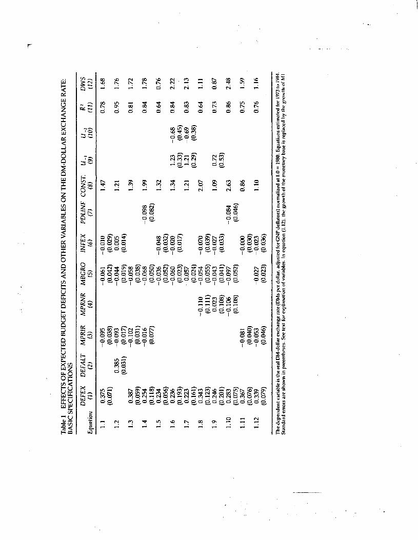
5. The Estimated Reduced Form EquationsTable 1 presents the basic reduced-form equation and a number of varia-tions on this specification. In equation (1.1) the coefficient of the ex-pected deficit variable (DEFEX) is 0.375 with a standard error of 0.071,implying that each percentage point increase in the ratio of expectedstructural deficit to GNP raises the real dollar-DM index by 0.375 points.As noted above, the real dollar-DM index rose from 0.99 in 1978—79 to1.72 in 1984 while the expected deficit rose from 1.68 percent of GNP to3.35 percent of GNP. The coefficient of 0.375 implies that the rise inDEFEX accounts for 63 points of the 73-point rise in the index.

The coefficient of the tax variable, the maximum potential real interestrate (MPRIR) supportable by a standard project, has the wrong sign. Iwill return later to this and to its sensitivity to specification.

The coefficient of the ARIMA inflation projection (INFEX) is negativebut is only —0.010 and much smaller than its standard error of 0.029. It isuseful to reiterate a point made earlier that this ARIMA variable shouldnot be regarded as equivalent to inflation expectations since inflation ex-pectations at any time will also reflect the growth of the monetary base,the size of projected budget deficits, and many other political and eco-nomic factors.

Tabl

e I

EFFE

CTS

OF

EXPE

CTE

D B

UD

GET

DEF

ICIT

S A

ND

OTH

ER V

AR

IAB

LES

ON

TH

E D

M-D

OLL

AR

EX

CH

AN

GE

RA

TE:

BA

SIC

SPE

CIF

ICA

TIO

NS

Equa

tion

DEF

EX(1

)D

EFA

LT(2

)M

PRIR

(3)

MPR

NR

(4)

MB

GR

O(5

)IN

FEX

(6)

PDLI

NF

(7)

CO

NST

.(8

)U

.., (9)

(10)

(11)

DW

S(1

2)

1.1

0;37

5—

0.09

5—

0.06

1—

0.01

01.

470.

781.

68(0

.071

)(0

.038

)(0

.042

)(0

.029

)1.

20.

385

(0.0

31)

—0.

093

(0.0

17)

—0.

044

(0.0

19)

0.00

5(0

.014

)1.

210.

951.

76

1.3

0.38

7—

0.10

2—

0.05

81.

390.

811.

72(0

.059

)(0

.031

)(0

.038

)1.

40.

254

—0.

016

—0.

068

—0.

098

1.99

0.84

1.78

(0.1

18)

(0.0

77)

(0.0

50)

(0.0

82)

1.5

0.23

4—

0.03

6—

0.04

81.

320.

640.

76(0

.056

)(0

.052

)(0

.032

)1.

60.

236

—0.

060

—0.

020

1.34

1.23

—0.

680.

842.

22(0

.193

)(0

.023

)(0

.017

)(0

.33)

(0.4

5).

1.7

0.22

3—

0.05

71.

211.

21—

0.69

0.83

2.13

(0.1

61)

(0.0

24)

(0.2

9)(0

.38)

1.8

0.34

3—

0.11

0—

0.05

4—

0.07

02.

070.

641.

11(0

.123

)(0

.111

)(0

.055

)(0

.039

)1.

90.

246

0.02

3—

0.04

3—

0.02

71.

090.

720.

730.

87(0

.201

)(0

.108

)(0

.041

)(0

.033

)(0

.53)

1.10

0.28

3—

0.10

6—

0.09

7—

0.08

42.

630.

862.

48(0

.075

)(0

.108

)(0

.052

)(0

.046

)1.

110.

367

—0.

081

—0.

000

0.86

0.75

1.59

(0.0

76)

(0.0

40)

(0.0

30)

.

1.12

0.33

9—

0.05

3—

0.02

7—

0.02

31.

100.

761.

16(0

.079

)(0

.046

)(0

.023

)(0

.036

).

The

dep

ende

ntva

riabl

e is

the

real

DM

-dol

lar

exch

ange

rat

e (D

Ms

per

dolla

r, a

djus

ted

for

GN

P d

etla

tors

) no

rmal

ized

at 1

.019

80. E

quat

ions

est

imat

ed fo

r 19

73 to

198

4.S

tand

ard

erro

rs a

re s

how

n in

par

enth

eses

. See

text

for

expl

anat

ion

of v

aria

bles

. In

equa

tion

(1.1

2), t

he g

row

th o

f the

mon

etar

y ba

se is

rep

lace

d by

thegr

owth

ol M

l

376 FELDSTEIN

Finally, the rate of growth of the monetary base has a coefficient of—0.06 (with a standard error of 0.042), implying that a faster rate ofmonetary growth depresses the value of the dollar.

The adjusted R2 of 0.78 implies that the equation explains the varia-tions in the dollar-DM ratio quite well and the Durbin-Watson statistic of1.68 indicates that there is little serial correlation of the residuals.

Equation (1.2) replaces the basic DEFEX variable with the alternativeDEFALT variable (described in section 3.1) that was constructed to avoidthe assumption that financial market participants anticipated the largebudget deficits before 1981. The coefficient of DEFALT is 0.385 and there-fore almost identical to the 0.375 coefficient of DEFEX reported in equa-tion (1.1). The standard error of DEFALT is, however, only 0.031 or lessthan half of the standard error of the coefficient of DEFEX, reflecting thefact that the alternative variable has far less "noise" in it. This is also seenin the sharp rise of the corrected from 0.78 in equation (1.1) to 0.95 inequation (1.2). The other coefficients are not changed in any substantialway. Although DEFALT seems clearly to be a better variable than theDEFEX variable, the latter does have the virtue that its construction in-volved less discretion and I will continue to present results for DEFEX.

Because the coefficient of the inflation variable is much smaller than itsstandard error, it is desirable to conserve the very scarce degrees of free-dom by reestimating the equation with the INFEX variable omitted. Thisis done in equation (1.3). None of the remaining coefficients or standarderrors changes appreciably.

Instead of omitting the rolling ARIMA forecast variable, equation (1.4)replaces it with a polynomial distributed lag on the annual changes ofthe GNP deflator. The distributed lag coefficients are constrained to sat-isfy a third-order polynomial on six lagged values of the annual rate ofchange of the GNP deflator with no restriction on the final weight. Thesum of the implied coefficients is —0.098 with a standard error of 0.082.The monetary base variable remains essentially unchanged with this re-specification. The coefficient of MPRIR drops to —0.016 and is com-pletely insignificant (standard error 0.077); this is reassuring since aninsignificant coefficient is quite plausible while a significantly negativeone cannot be justified. Finally, the coefficient of DEFEX drops to 0.254but remains both statistically significant and economically very power-ful. The corrected R2 statistic of 0.84 shows that the polynomial dis-tributed lag specification has slightly greater explanatory power than themore constrained INFEX specification.

Since the MPRIR variable is either insignificant or significant with thewrong sign, it is useful to see the implications of omitting it from thespecification. This is done in equation (1.5). The coefficient of the DEFEX

The Budget Deficit 377

variable is 0.234, indicating that the decline in the coefficient value ob-served in equation (1.4) was due to the small size of the MPRIR coef-ficient rather than to the change in the inflation variable per Se. Thisspecification is clearly inferior to the previous ones, with a much lowercorrected and a very much lower Durbin-Watson statistic.

To deal with the low Durbin-Watson statistic, equation (1.5) was re-estimated with a first-order transformation. Since this still had a lowDurbin-Watson statistic, a second-order autocorrelation correction wasused. This is shown in equation (1.6). The DEFEX coefficient has re-mained essentially unchanged at 0.236 and the MBGRO coefficient hasreturned to —0.060. The inflation coefficient is now the same size as itsstandard error. This variable is dropped in equation (1.7) where theother coefficients remain essentially unchanged.

The specification of the MPRIR variable requires assuming a particularmarginal debt-equity ratio and a particular yield difference betweenequity and debt. An alternative measure of the effect of changes in taxrules and in the tax-inflation interaction is to use the less restricted vari-able MPRNR, the maximum potential real net return. This alternative isused in equations (1.8) through (1.10).

Equation (1.8) parallels (1.1) except for the substitution of MPRNR forMPRIR. The DEFEX variable is essentially unchanged (0.343 with astandard error of 0.123) while the MPRNR is statistically insignificant.MBGRO is similar to its earlier value (—0.054) and the INFEX variableis now nearly twice its standard error (—0.070 with a standard errorof 0.039). A first-order autocorrelation correction actually lowers theDurbin-Watson statistic.

A far better specification is obtained by substituting the polynomialdistributed lag for the INFEX variable (equation 1.10). This combinationof variables has the highest corrected R2 statistic (0.86) of all the regres-sions that include the DEFEX variable and a Durbin-Watson statistic of2.48. The coefficient of the DEFEX variable is 0.283 with a standard errorof only 0.075. MBGRO and PDLINF are both negative and nearly twicetheir standard errors while the coefficient of MPRNR is satisfactorily lessthan its standard error.

Equation (1.11) is similar to (1.1) but constrains the monetary basegrowth not to appear in the equation. Although the resulting specifica-tion is not very satisfactory, the coefficient of DEFEX remains almost un-changed from equation (1.1).

Finally, equation (1.12) substitutes the rate of growth of Ml for the rateof growth of the monetary base. The coefficients are generally similar tothose of equation (1.1) but the overall goodness of fit is slightly worse.

A variety of additional sensitivity tests are presented in table 2. These

Tabl

e 2

EFFE

CT

OF

AD

DIT

ION

AL

VA

RIA

BLE

S O

N T

HE

ESTI

MA

TED

EFF

ECF

OF

THE

EXPE

CTE

D B

UD

GET

DEF

ICIT

S O

NTH

E D

M-D

OLL

AR

EX

CH

AN

GE

RA

TE

Equ

atio

nD

EFEX

(1)

MPR

IR(2

)M

PRN

R(3

)M

BG

RO

(4)

INFE

X(5

)PD

LJN

F(6

)D

UM

8O+

(7)

GN

PGR

O(8

)N

IJP

(9)

CO

NST

.(1

0)R

2(1

1)D

WS

(12)

2.1

0.52

5—

0.07

3—

0.06

5—

0.01

2—

0.28

31.

170.

841.

77(0

.099

)(0

.034

)(0

.035

)(0

.025

)(0

.147

)2.

20.

539

—0.

081

—0.

061

—0.

281

1.07

0.86

1.77

(0.0

89)

(0.0

28)

(0.0

32)

(0.1

38)

2.3

0.45

4—

0.05

9—

0.05

7—

0.03

2—

0.22

41.

310.

862.

33(0

.185

)(0

.078

)(0

.047

)(0

.091

)(0

.167

)2.

40.

484

—0.

048

—0.

037

—0.

386

0.95

0.77

1.46

(0.1

19)

(0.0

42)

(0.0

26)

(0.1

70)

2.5

0.55

3—

0.08

4—

0.06

2—

0.05

5—

0.36

51.

540.

761.

43(0

.142

)(0

.092

)(0

.045

)(0

.033

)(0

.173

).

2.6

0.34

3—

0.06

7—

0.09

4—

0.17

41.

730.

871.

72(0

.107

)•

(0.0

43)

(0.0

37)

(0.1

46)

.

2.7

0.42

9—

0.17

3—

0.07

7—

0.02

90.

034

2.09

0.71

1.05

(0:1

22)

(0.1

07)

(0.0

51)

(0.0

43)

(0.0

21)

2.8

0.36

5—

0.18

3—

0.10

3—

0.05

40.

017

2.72

0.86

2.34

(0.1

11)

(0.1

33)

(0.0

53)

(0.0

55)

(0.0

17)

2.9

0.64

2—

0.14

7—

0.08

5—

0.01

4—

0.36

80.

634

1.56

0.87

1.56

(0.1

10)

(0.0

72)

(0.0

34)

(0.0

29)

(0.1

27)

(0.0

14)

2.10

0.54

7—

0.06

9—

0.07

2—

0.02

2—

0.30

10.

022

0.88

0.89

1.63

(0.0

85)

(0.0

29)

(0.0

30)

(0.0

28)

(0.1

25)

(0.0

12)

2.11

0.24

1—

0.06

9—

0.11

30.

004

2.01

0.84

1.51

(0.0

70)

(0.0

50)

•(0

.038

)(0

.016

)2.

120.

346

—0.

100

—0.

049

—0.

068

•0.

003

1.92

0.59

1.12

(0.1

35)

(0.1

47)

(0.0

70)

(0.0

45)

(0.0

27)

•

The

depe

nden

t var

iabl

e is

the

real

DM

-dol

lar e

xcha

nge

rate

(DM

a pe

r dol

lar,

adju

sted

for G

NP

defla

tors

) nor

mal

ized

at 1

.0 =

1980

.Eq

uatio

ns e

stim

ated

for 1

.973

to 1

984.

Stan

dard

err

ors a

re sh

own

in p

aren

thes

es. S

ee te

xtfo

rex

plan

alio

n of

var

iabl

es.

The Budget Deficit 379

tests involve adding several new variables as well as considering some ofthe variations discussed in table 1. All of the results again support theconclusion that the coefficient of the expected deficit is statistically sig-nificant and economically powerful.

Equation (2.1) starts with the basic specification of equation (1.1) andadds a dummy variable equal to one for the years 1980 through 1984 andzero for the previous years. The purpose of the dummy variable is to testwhether the dollar was strong in the 1980s for any of a variety of other-wise unspecified reasons (the new monetary policy regime that began inOctober 1979; the Reagan presidency; the increased importance of theUnited States as a political safe haven for foreign capital). if some com-bination of omitted variables did indeed raise the dollar in the 1980sabove what it would otherwise have been, the equations of table 1 mighthave imputed this to the large expected deficits or to some other variablethat distinguished the 1980s from previous years. Including a specificdummy variable should eliminate this source of bias.

Rather surprisingly, the coefficient of the dummy variable for the 1980s(DUM8O+) is negative, about twice its standard error and quite large inabsolute size (about —0.25). This implies that the unspecified factors atwork in the 1980s had the effect of lowering the dollar relative to the Ger-man mark in comparison to the earlier years. Faced with the negativeco-efficient, it is of course possible to identify possible explanations. For•example, the decline in OPEC financial assets during most of the 1980sreduced the demand for dollar securities relative to DM securities. Theconservative political victories in Germany and Britain, and the switch inFrench economic policy, may have revived the demand for portfolio in-vestment in Europe.

The important point to note about these arguments is that they implythat the actual rise of the dollar in the 1980s is even more surprising andthat the combined role of those factors that systematically raised the dol-lar was even stronger. The other coefficients of equation (2.1) show thatthe primary effect of including DUM8O+ is to raise the coefficient ofDEFEX from 0.375 to 0.525.

The DUM8O+ variable appears in most of the specifications of table 2.Its coefficient is almost always about twice its standard error and it hasthe effect of raising the coefficient of DEFEX to 0.5 or above. Although itis of course possible that the DUM8O+ variable is spurious, it is not nec-essary to decide this question in order to say whether the rise in theexpected budget deficit was an important cause of the increase in thedollar. That is dearly an implication of the specifications of tabel 1 with-out the DUM8O+ variable as well as of the equations in table 2 with theDUM8O+ variable.

FELDSTEIN

Equation (2.2) drops the INFEX variable and equation (2.3) replaces itwith the polynomial distributed lag. Equation (2.4) omits the tax variablewhile equation (2.5) switches to the relatively unconstrained MPRNRspecification. Equation (2.6), with no tax variable and with the distrib-uted lag specification of the inflation variable is one of the few specifica-tions in which the coefficient of the DUM8O+ variable is only slightlygreater than its standard error. In this specification, the coefficient of theDEFEX variable is reduced to the level of 0.343, approximately its valuein the equations without the DUM8O+ variable.

Equations (2.7) through (2.11) include the annual growth of real GNP(GNPGRO) as an additional explanatory variable. When the DUM8O+variable is not present (equations 2.7 and 2.8), the GNPGRO variableis only slightly greater than its standard error. The DEFEX coefficientsare raised by a small amount and the inflation variables are insignifi-cant. When the DUM8O+ variable is present, the GNPGRO coefficientsare quite significant and the DEFEX coefficients are increased to morethan 0.5.

Finally, equation (2.2) adds the net international investment positionof the United States as a percent of GNP (NH!'.). Its coefficient is verymuch less than its standard error and the remaining coefficients are verysimilar to the coefficients of equation (1.8) (which has the same specifica-tion except for the NHP variable). The statistical insignificance of this co-efficient should not be overinterpreted. As I noted above, the net stockof accumulated assets may not be truly exogenous since the decline inNH!' in the 1980s has been the cumulative result of the high value of thedollar and the resulting current account deficits.'3

Table 3 extends the analysis of tables 1 and 2 to include the Germandeficit and monetary base variables. For reference, the basic specifica-tion of equation (1.1) is repeated in equation (3.1). Adding the variablethat measures the ratio of expected German deficits to GNP (DEFEXG)and the growth of the German monetary base (MBGROG) does not alterthe other coefficients subtantially but does cause the standard errors tobecome quite large (equation (3.2)). The additional variables also leavethe corrected R2 unchanged.

The increased standard errors are perhaps not surprising since equa-tion (3.2) has six coefficients and a constant term to estimate with onlytwelve observations. Dropping the German monetary base variable

13. When equation (2.12) was estimated with the stock of foreign private assets in theUnited States as a percentage of GNP instead of NIIP, its coefficient had the wrong sign(positive) and was statistically significant. This again no doubt reflects the fact that for-eign private investment in the United States grew in the 1980s because of the highdollar.

Tabl

e 3

EFFE

CTS

OF

US

AN

D G

ERM

AN

EX

PEC

TED

BU

DG

ET D

EFIC

ITS

AN

D O

THER

VA

RIA

BLE

S O

N T

HE

DM

-DG

1.LA

REX

CH

AN

GE

RA

TE

Equa

tion

DEF

EX(1

)D

EFA

LT(2

)M

PRIR

(3)

MB

GR

O(4

)IN

FEX

(5)

DEF

EXG

(6)

MB

GR

OG

(7)

CO

NST

.(8

)(9

)U

2(1

0)R

2(ii

)D

WS

(12)

3.1

0.37

5—

0.09

5—

0.06

1—

0.01

01.

470.

781.

68(0

.071

)(0

.038

)(0

.042

)(0

.029

)3.

20.

344

—0.

100

—0.

081

0.02

8—

0.05

50.

040

1.22

0.78

1.85

3.3

(0.4

91)

0.32

3(0

.044

)—

0.09

3(0

.046

)—

0.06

2(0

.051

)—

0.00

7(0

.217

)0.

022

(0.0

30)

1.58

0.75

1.64

(0.5

21)

(0.0

47)

(0.0

47)

(0.0

47)

(0.2

18)

3.4

0.41

4(0

.103

)—

0.09

2(0

.018

)—

0.04

5(0

.025

)0.

010

(0.0

23)

0.00

7(0

.055

)0.

009

(0.5

09)

1.06

0.94

1.76

3.5

0.20

2(0

.058

)—

0.02

9(0

.012

)—

0.17

3(0

.087

)1.

151.

73(0

.11)

—0.

94(0

.09)

0.95

2.11

3.6

0.21

2(0

.070

)—

0.03

4(0

.016

)—

0.01

6(0

.013

)—

0.06

7(0

.154

)1.

211.

60(0

.37)

—0.

91(0

.15)

0.96

1.84

The

dep

ende

nt v

aria

ble

is th

e re

al D

M-d

olla

r ex

chan

ge r

ate

(DM

s pe

r do

llar,

adp

uste

d fo

r G

NI'

defla

tors

) no

rmal

ized

at 1

.0 =

198

0. E

quat

ions

est

imat

ed fo

r 19

73to

198

4.S

tand

ard

erro

rs a

re s

how

n in

par

enth

eses

. See

text

for

expl

anat

ion

of v

aria

bles

.

FELDSTEIN

(equation (3.3)) leaves the coefficients of the four U.S. variables very.similar to the basic specification of equation (3.1) but with very largestandard errors. The coefficient of the German deficit variable is smalland only about one-tenth of its standard error.

In an attempt to reduce the problem of the large standard errors, theseequations are repeated with the standard DEFEX variable replacedby the alternative DEFALT variable in which the observations for 1977through 1980 are modified to assume that the 1980 deficit-GNP ratio wasprojected forward until after the 1980 election. Equation (1.2) indicatedthat this substitution leaves the coefficient of the deficit and other vari-ables essentially unchanged while reducing their standard errors. Theeffect is similar in equation (3.4). The coefficient of DEFALT is 0.414 witha standard error of 0.103. The coefficients of MPRIR and MBGRO arevery similar to their values in equation (3.1) but with smaller standarderrors. The coefficient of INFEX remains very much smaller than its stan-dard error. The coefficients of the two German variables are again muchsmaller than their standard errors.

Dropping the insignificant MBGROG and INFEX variables and theMPRIR variable which has an inadmissible sign lead to equation (3.5) inwhich the three remaining variables are statistically significant and havethe correct sign. In this equation, which is estimated after a second-orderautocorrelation transformation, the coefficient of DEFALT is 0.202 (witha standard error of 0.058) and in which the coefficient of the Germandeficit variable is —0.173 with a standard error of 0.087.

This coefficient structure is, however, quite fragile. Adding the INFEXvariable produces a coefficient of —0.016 with a standard error of 0.013while the coefficient of the German deficit variable drops to —0.067 andless than half of its standard error.

In short, it seems from table 3 that the German deficit variable doesnot have a significant or stable relation to the dollar-DM ratio and thatthe decision of whether or not to include it does not alter the point esti-mate of the U.S. deficit variable. Future work will be needed to assesswhether some combination of German and other European deficits issignificant and whether its presence alters the coefficient of the U.S.budget deficit variable.

It is, of course, unfortunate that the history of the floating rate periodgives us only twelve years of experience to analyze. Although more datapoints could be created by using quarterly observations, I believe verylittle (if any) additional information on DEFEX and MPRIR would actu-ally result. Instead, there would be more measurement error in the"expectations" variables (DEFEX, INFEX, MPRJR) relative to the actualvariation. Looking back before 1973 is inappropriate because the quasi-

r

The Budget Deficit 383

fixed rate system that existed then would imply very different exchange-rate dynamics and might be expected to have very different monetarypolicy responses as countries tried to maintain their currencies at thefixed parities. Expectations would also be formed differently in a regimein which governments were committed to maintaining fixed exchangerates and in which the United States appeared willing to accumulateoverseas investments or run down its assets in order to maintain thatfixed rate system.

6. Effects of the Interest DifferentialI have already commented (in section 2) on the difficulty of assessing thestructural relation between the exchange rate and the difference in ex-pected real interest rates. The expected inflation rate, which is a verycritical component of the calculation, is difficult to measure and the realinterest rates themselves are endogenous variables.

Despite these difficulties, it is worth devoting some attention to the es-timation of a structural equation linking the exchange rate to the realinterest differential because it is the operational link between budgetdeficits and the exchange rate in several analytic models. The prob-lems of measurement and of endogeneity can be mitigated by using aninstrumental variable procedure with the DEFEX, MBGRO, and INFEXvariables as the instruments. The results indicate that the use of an in-strumental variable procedure is important and that, when it is used, theevidence shows a substantial effect of the real interest differential on theexchange rate.

Equation (4.1) of table 4 presents an ordinary-least-squares regressionof the exchange rate index on the difference between the real long-terminterest rate in the United States and a corresponding real long-term in-terest rate for Germany. The nominal U.S. rate is the yield on Treasurybonds with five years to maturity. The real rate is calculated by subtract-ing the ARIMA projection (INFEX) from this nominal rate. The nominalGerman rate is a rate on long-term German government bonds.'4 The realrate is calculated by subtracting an ARIMA estimate of future Germaninflation calculated by the same process used for the U.S. ARIMA fore-cast of inflation. Annual values of these variables are shown in appendixtable A-2.

The coefficient of the real interest rate differential is 0.042 with a stan-dard error of 0.025. The Durbin-Watson statistic is very low and the

14. The German interest rate was provided by Data Resources, Inc. and is identified byData Resources as RMGBL@GY.

'Rea

l int

eres

t is

inte

rest

min

us A

RIM

A p

redi

ctio

ns o

f inf

latio

n.

The

dep

ende

nt v

aria

ble

is th

e re

al D

M-d

olla

r ex

chan

ge r

ate

(DM

s pe

r do

llar,

adj

uste

d fo

r C

NP

def

lato

rs)

norm

aliz

ed a

tpa

rent

hese

s. S

ee te

xt lo

t exp

lana

tion

of v

aria

bles

.1.

0 =

198

0. S

tand

ard

erro

rs a

re s

how

n in

Tabl

e 4

REA

L IN

TER

EST*

DIF

FER

ENTI

ALS

AN

D T

HE

DM

-DO

LLA

R E

XC

HA

NG

E R

ATE

Estim

atio

n

inte

rest

Rat

es m

inus

Pred

icte

d In

flatio

n

U_2

R2

(SER

)D

WS

RU

S-R

GR

US

RG

Con

stan

tEq

uatio

nM

etho

dIn

terv

al(1

)(2

)(3

)(4

)(5

)(6

)(7

)(8

)

4.1

OLS

1973

—84

0.04

2(0

.025

)1.

240.

14(0

.21)

0.41

4.2

OLS

1973

—84

0.03

21.

320.

810.

630.

90A

RI

(0.0

23)

(0.1

9)(0

.13)

4.3

OLS

1973

—84

0.03

41.

261.

27—

0.59

0.74

2.13

AR

2(0

.022

)(0

.29)

(0.3

1)(0

.11)

4.4

IV19

73—

840.

082

1.25

NA

0.53

(0.0

35)

(0.2

3)4.

5IV

1973

—84

0.05

41.

260.

75N

A1.

18A

RI

(0.0

23)

(0.1

8)(0

.15)

4.6

OLS

1973

—84

0.05

1(0

.024

)0.

003

(0.0

37)

1.08

0.23

(0.1

9)0.

48

4.7

OLS

1973

—84

0.03

80.

011

1.10

1.38

—0.

750.

802.

08A

R2

(0.0

19)

(0.0

34)

(0.2

8)(.0

28)

(0.1

0)4.

8IV

1973

—84

0.08

0(0

.034

)—

0.00

5(0

.061

)1.

17N

A(0

.16)

1.05

4.9

IV19

73—

840.

046

—0.

037

1.23

0.74

NA

1.05

AR

I(0

.024

)(0

.024

)(0

.18)

(0.1

6)

The Budget Deficit 385

equation is reestimated with an autocorrelation transforma-tion. A first-order transformation (equation (4.2)) is inadequate so thefinal result (presented in equation (4.3)) has a second-order autocorrela-tion correction. In this form, the coefficient of the interest differential is0.034 with a standard error of 0.022.

When the equation is estimated by art instrumental variable procedure(equation (4.4)), the coefficient of the interest rate differential becomesmuch larger (0.082) and more than twice its standard error. The Durbin-Watson statistic is, however, very small (0.56). When Fair's method isused to obtain an instrumental variable estimate with a first-order auto-correlation correction, the coefficient falls to 0.054 with a standard errorof 0.023. In short, the instrumental variable procedure results in a slightlylarger coefficient than the OLS procedure. It might also be noted thatthese coefficient estimates are similar to the estimates of approximately0.06 obtained by Sachs (1985) and Hooper (1985).

Before looking at any further equation estimates, it is helpful to con-sider the implications of a coefficient of approximately 0.04 to 0.06 on theinterest rate differential. In 1978—79, the estimated real long-term U.S.rate exceeded the corresponding German rate by 0.7 percent; by 1983 thedifferential was 1.4 percent and by 1984 it was 2.8 percent. Even a coeffi-cient of 0.06 implies a rise in the dollar-DM real exchange rate of 0.042between 1980 and 1983 and of 0.126 between 1980 and 1984. Since theactual exchange rate rose by 0.72 points over this period, the equationcan account for at most one-fifth of the actual rise.

The estimated coefficient is far less than theory suggests. An increaseof one percentage point in the difference between U.S. and German 10-year real interest rates should increase the dollar-DM exchange rate byabout twelve percentage points, not the four to six percentage points es-timated here and in previous studies. This implies that the coefficientmay be grossly underestimated because of the measurement and simul-taneity problems referred to above.

When the interest differential is split into two separate interest ratesand the equation estimated by ordinary least squares, only the coeffi-cient of the U.S. rate is statistically significant. This remains true whenthe equation is reestimated with a second-order autocorrelation correc-tion (equation (4.7)) and by an instrumental variable procedure (equa-tion (4.8)).

However, the combination of instrumental variable estimation and afirst-order autocorrelation correction (Fair's method) does result (equa-tion (4.9)) in coefficients for the U.S. and German interest variables thatare both absolutely about 0.04 but with the appropriate opposite signs.More specifically, the coefficient of the real U.S. rate is 0.046 (with a stan-

FELDSTEIN

dard error of 0.024) while the coefficient of real German rate is —0.037(with a standard error of 0.024).

As an alternative to the rolling ARIMA procedure, I have also used asimpler method that may correspond more closely to the way that marketparticipants used past inflation experience to form judgments about thefuture. In place of the ARIMA estimate of inflation, I use a weightedaverage of inflation, giving a weight of 0.5 to the most recent year's infla-tion, of 0.33 to the inflation of the previous year's inflation and of 0.17 tothe inflation of the year before that. On that basis, the expected inflationcame down gradually in Germany from 4.5 percent in 1980 to 4.3 percentin 1981 and 1982, 3.8 percent in 1983, and 2.8 percent in 1984, and realGerman long-term rates in the 1980—84 period stayed between 4.0 and5.0 percent except for a 6.1 percent rate in 1981.

Table 5 presents the results based on this simpler specification of ex-pected inflation. The OLS estimates (equations (5.1) and (5.2)) are simi-lar to the estimates with the ARIMA inflation forecast: a coefficient of0.055 with a standard error of 0.035. The instrumental variable estimates(equations (5.3) and (5.4)) show a more substantial coefficient and asmaller standard error of regression measures than the ARIMA forecast.With the AR1 correction (i.e., using Fair's method), the coefficient of theinterest differential is 0.081 with a standard error of 0.031. This is ap-proximately twice the typical estimate based on the ARIMA inflationforecast. Dividing the interest differential into a real U.S. rate and a realGerman rate (equation (5.5)) results in a coefficient of 0.072 (with a stan-dard error of 0.025) for the U.S. real rate but a very small and statisticallyinsignificant coefficient of 0.003 (with a standard error of 0.032) for theGerman real rate, possibly because there was very little variation in themeasured real rate for Germany.

In short, the different specifications of the real interest differentialsand the different estimation methods indicate that each percentage pointdifference in real interest rates raises the real exchange rate by between0.04 and 0.08 points, an impact that accounts for only a small part of therise in the exchange rate that actually occurred in the 1980s and also onlya small part of the rise in the exchange rate that is predicted by thechanges in the expected budget deficits and in monetary policy. It isdifficult to tell whether this is because the real interest differential ismeasured very badly (causing a substantial underestimate of the true co-efficient) or because the budget deficit and monetary policy have directeffects on the exchange rate that are not channeled through the real in-terest differential.

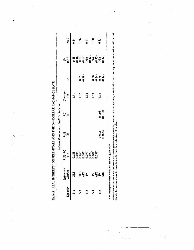
Tabl

e 5

REA

L IN

TER

EST*

DIF

FER

ENTI

ALS

AN

D T

HE

DM

-DO

LLA

R E

XC

HA

NG

E R

ATE

Estim

atio

n

Inte

rest

Rat

es m

inus

Pred

icte

d in

flatio

n

RU

S-R

GR

US

RG

Con

stan

tE

quat

ion

Met

hod

(1)

(2)

(3)

(4)

U_1

(SER

)D

WS

5.1

OLS

0.05

5(0

.035

)1.

310.

45(0

.16)

0.84

5.2

OLS

AR

10.

055

(0.0

35)

1.32

0.69

(0.7

8)0.

62(0

.14)

1.36

5.3

IV0.

097

(0.0

29)

1.32

NA

(0.1

7)0.

91

5.4

IV AR

10.

081

(0.0

31)

.

1.33

0.58

(0.2

4)N

A(0

.15)

1.50

5.5

IV AR

I0.

072

(0.0

25)

0.00

3(0

.033

)1.

040.

75(0

.17)

NA

(0.1

2)0.

83

* R

eal i

nter

est i

s in

tere

st m

inus

dis

trib

uted

lag

infla

tion.

The

dep

ende

nt v

aria

ble

is th

e re

al D

M-d

olla

r ex

chan

ge r

ate

(DM

s pe

r do

llar,

adj

uste

d fo

r G

M' d

efla

tors

) no

rmal

ized

at 1

.0 =

198

0. E

quat

ions

est

imat

ed b

r 19

73to

198

4.S

tand

ard

erro

rs a

re s

how

n in

par

enth

eses

. See

text

for

expl

anat

ion

of v

aria

bles

.

-1

r

388 FELDSTEIN

7. Concluding Comments

The findings of the current research can be summarized briefly. The esti-mated reduced-form equations for the dollar-DM real exchange rateimply that the rise in the expected future deficits in the budget of theU.S. government had a powerful effect on the exchange rate between thedollar and the German mark. Each one percentage point increase inthe ratio of future budget deficits to GNP increases the exchange rate byabout thirty percentage points.

Changes in the growth of the monetary base also affect the exchangerate, but the estimated effect of the deficit does not depend on whetherthis is taken into account in the estimation procedure.

The analysis also indicates that the changes in tax rules and in theinflation-tax interaction that altered the corporate demand for funds didnot have any discernible effect on the exchange rate. The presence or ab-sence of alternative tax variables did not alter the estimated effect of thebudget deficit.

The estimated effect of the budget deficit is also relatively insensitiveto the other variables that were induded in the regression equation.

As I have emphasized elsewhere in a different context (Feldstein 1982),all models are "false" in the sense that they involve substantial sim-plifications that can lead to incorrect inferences. It is impossible to relaxall of the specification constraints or include all of the plausible variablesin any single model. We learn about reality only by examining a varietyof alternative false models to see which implications of these models arerobust. In the present study, I was eager to focus on the question ofwhether changes in the expected budget deficit could account for shiftsin the real exchange rate and, if so, whether this was a spurious relationthat was really reflecting a more fundamental relationship between theexchange rate and tax rules, monetary policy, inflation, German budgetdeficits, or unobservable characteristics of the 1980s that strengthenedthe dollar. Although any econometric study leaves room for doubt anduncertainty, I believe that the current evidence shifts the burden of proofto those who would claim that deficits do not matter or that tax, mone-tary, or "confidence" variables were the real reasons for the dollar'sstrength since 1980.

There are of course a number of things that have been omitted fromthe analysis that deserve attention in future studies. It would be good tomodel the changing behavior of expected European budget deficits or,even more generally, the changing balance between the supply and de-mand for funds in Europe. There are a number of difficulties in doing so,

The Budget Deficit 389

including the problem of establishing the "full employment" level atwhich to estimate structural deficits in the face of Europe's rapidly risingunemployment and the much larger and more ambiguous role of publicinvestment in Europe.

U.S. budget deficits have been defined without correction for the in-flation erosion of the public debt on the implicit assumption that, at theobserved rates of inflation, individuals did not adjust their saving buttreated the inflation component of the interest on the public debt asincome.

Shifts in the price of oil were ignored in the present study althoughthey presumably affected the equilibrium exchange rate between the DMand the dollar. It should be possible to extend the analysis to include theprice of oil and other raw materials.

Finally, in future work I plan to extend the analysis to include 1985 andthe decline of the dollar. The sharp rise in the dollar-DM ratio that cli-maxed in the early spring of 1985 may have had some unsustainablespeculative element (as Krugrnan's 1985 analysis implies) but the declineof more than 20 percent in the dollar-DM ratio between mid-1984 and thepresent time is, I believe, quite in line with what would have been ex-pected on the basis of the fall in expected future budget deficits.

As participants in financial markets studied the action of Congress inthe spring and early summer of 1985, there was growing confidence thatsome significant action would be taken to reduce future budget deficits.The Congressional Budget Office summarized this in August when itcontrasted the current services deficits of 5.1 percent of GM? each yearfrom 1986 to 1990 with the results of the Congressional Budget Resolu-tion that brought the projected deficits onto a path that declined to 3.0percent of GNP in 1988 and 2.1 percent in 1990. The Gramm-Rudmanamendment gave the markets even greater confidence that budget defi-cits would continue to decline in the future.

The estimated ratio of the expected 5-year structural deficit to poten-tial GM? has declined from 3.3 percent in 1984 (the last observation inthe sample) to about 2.6 percent in early 1986. An estimated coefficientof 0.25 to 0.40 would imply a decline in the dollar from this source aloneof between 18 and 28 points. In fact, as of mid-February 1986, the dollar-DM ratio was down 23 points in comparison to its 1984 average value and32 points from its high in early 1985.

There is substantial room for additional research on the determinantsof the exchange rate. But the massive fiscal experiment of the past sixyears should have convinced us that sustained shifts in the federal gov-ernment's deficit have powerful effects on the value of the dollar.

Tabl

e A

-iTI

ME

SER

IES

REG

RES

SIO

N V

AR

IAB

LES

DM

-D

olla

rIn

dex

DEF

EX D

EFA

LT M

PRJR

MPR

NR

MB

GR

O M

IGR

O IN

FEX

GN

PGR

ON

IIP

DEF

EXG

•MB

GR

OG

Yea

r(1

1)(2

)(3

)(4

)(5

)(6

)—

(7)

(8)

(9)

(10)

(11)

(12)

1973

1.20

81.

802

1.80

23.

500

5.80

08.

348

5.75

64.

500

5.19

811

.659

—1.

220

10.6

3719

741.

189

1.82

91.

829

4.10

05.

000

8.09

14.

761

7.50

0—

0.53

910

.893

—1.

820

6.12

119

751.

166

1.80

81.

808

5.30

05.

100

7.68

15.

014

9.70

0—

1.25

711

.171

—2.

180

7.84

319

761.

211

1.65

11.

651

4.40

06.

000

7.52

06.

141

5.80

04.

887

10.2

51—

2.00

09.

245

1977

1.14

01.

519

1.62

34.

400

6.00

08.

045

8.12

26.

000

4.66

68.

453

—2.

040

8.97

519

781.

015

1.57

71.

615

4.60

05.

900

9.30

28.

222

6.40

05.

293

6.79

3—

1.96

08.

468

1979

0.96

81.

790

1.63

65.

500

6.10

08.

368

7.53

27.

000

2.47

86.

053

—1.

520

8.48

519

801.

000

2.33

51.

753

6.00

05.

900

8.16

97.

477

7.60

0—

0.16

65.

626

—0.

720

4.83

119

811.

310

2.82

12.

821

8.30

07.

200

6.43

25.

134

8.00

01.

936

5.24

30.

220

4.42

119

821.

430

3.24

73.

247

7.70

07.

500

6.85

28.

747

7.00

0—

2.54

94.

801

1.24

04.

933

1983

1.51

13.

377

3.37

77.

100

7.50

09.

483

10.3

875.

600

3.44

93.

116

1.96

07.

309

1984

1.71

63.

330

3.33

04.

900

7.30

08.

142

5.22

15.

500

6.61

9—

0.03

62.

400

4.76

9

The Budget Deficit• 391

Table A-2 INTEREST AND INFLATION TIME SERIES OBSERVATIONS

YearILlS(1)

JG(2)

INFPUSAR1MA

(3)

INFPGARIMA

(4)

INFPUSPAST

(5)

1NFPGPAST

(6)

1973 6.868 9.323 4.500 4.869 5.093 6.3131974 7.802 10.383 7.500 5.494 7.037 6.5551975 7.766 8.483 9.700 6.101 8.535 6.4051976 7.179 7.800 5.800 6.125 7.173 4.9821977 6.990 6.158 6.000 5.603 6.193 4.0621978 8.318 5.733 6.400 5.284 6.500 3.9901979 9.518 7.425 7.000 4.902 7.770 4.0531980 11.478 8.500 7.600 4.812 8.725 4.4621981 14.236 10.383 8.000 4.495 9.324 4.2881982 13.006 8.950 7.000 4.050 7.751 4.3201983 10.796 7.892 5.600 4.048 5.520 3.8021984 12.241 7.775 5.500 3.874 4.159 2.771

IUS = yield on 5-year government bonds;IG = yield on long-term German government bonds;INFPUS (ARIMA) = U.S. inflation predicted by ARJMA method;INFPG (ARIMA) = German inflation predicted by ARIMA method;INFPUS (PAST) = U.S. inflation predicted by average of past values;INFPG (PAST) = German inflation predicted by average of past values.

I am grateful to Andrew Berg for help with this work and to Rudiger Dornbusch, Jeff reyFrankel, Paul Krugman and Jeffrey Sachs for discussions about this subject.

REFERENCES

Barro, R. 1974. Are government bonds net wealth? Journal of Political Economy(November). 82: 1095—118..

Blanchard, 0. 1985. Debts1 deficits and finite horizons. Journal of Political Econ-omy 93 (April): 223—47.

Blanchard, 0., and L. Summers. 1985. Perspectives on high world real interestrates. Brookings Papers on Economic Activity 273—324.

Branson, W. 1985. Causes of appreciation and volatility of the dollar. NBERWorking Paper 1777.

Dombusch, R. 1976. Expectations and exchange rate dynamics. Journal of PoliticalEconomy (December). 84: 1161—76.

1983. Comment on floating exchange rates after ten years. BrookingsPapers on Economic Activity 1983: 1

Evans, P. 1985. Do large deficits produce high interest rates?" American EconomicReview 75 (March): 68—87.

1986. Is the dollar high because of large budget deficits? Journal of Mone-tary Economics. Forthcoming.

Feldstein, M. 1982. Inflation, tax rules and investment: Some econometric evi-dence. (The 1980 Fisher-Schultz Lecture of the Econometric Society), Econo-metrica 50(4): 825—62.

1983. Why the dollar is strong. In Foreign Exchange Value of the Dollar,

392 FELDSTEIN

Hearings Before the Committee on Banking, Finance and Monetary Policy,House of Representatives, October 1985 (reprinted in Challenge Magazine, 1984).

1985. American economic policy and the world economy. Foreign Affairs63 (Summer): 995—1008.

• 1986a. U.S. budget deficits and the European economies: Resolving thepolitical economic puzzle. American Economic Review 76 (May).

• 1986b. Budget deficits, tax rules and real interest rates. NBER WorkingPaper (Forthcoming).

Feldstein, M., and P. Bacchetta. 1986. U.S. budget deficits and European unem-ployment: The German experience. Forthcoming.

Feldstein, M., and L. Summers. 1978. Inflation, tax rules and the long-term in-terest rate. Brookings Papers on Economic Activity 1 (January): 61—99.

Feldstein, M., and J. Jun. 1986. The effects of tax rules on nonresidential fixedinvestment: Some preliminary evidence from the 1980s. Forthcoming inM. Feldstein, ed., Taxation and Capital Formation.

Frankel, J. 1979. On the mark: A theory of floating exchange rates based on realinterest differentials. American Economic Review 69 (September): 610—22.

1982. A test of perfect substitutability in the foreign exchange market.Southern Economic Journal 49 (October): 406—16.

1985. Causes of appreciation and volatility of the dollar. NBER WorkingPaper 1377.

Frenkel, J., and A. Razin. 1984. The international transmission of fiscal error andbudget deficits in the world economy. NBER Working Paper 1527.

1986. The international transmission and effects of fiscal policies. NBERWorking Paper 1799.

Hooper, P. 1985. International repercussions of the U.S. budget deficit. Brook-ings Discussion Paper 27 (February).

Hutchinson, M., and A. Throop. 1985. U.S. budget deficits and the real value ofthe dollar. Economic Review of the Federal Reserve Bank of San Francisco, Fall.

Krugrnan, P. 1985. Is the strong dollar sustainable? NBER Working Paper 1644.McKinnon, R. 1984. An international standard for monetary stabilization. Policy

Analyses in International Economics No. 8, Institute for International Economics.Meese, R., and K. Rogoff. 1983. Empirical exchange rate models of the seventies:

Do they fit out of sample? Journal of International Economics 14: 3—24.1985. Was it real? The exchange rate—interest differential relation, 1973—

1984. NBER Working Paper 1732.Obstfeld, M. 1985. Floating exchange rates: Experience and prospects. Brookings

Papers on Economic Activity 2: 369—450.Plosser, C. 1982. Government financing decisions and asset returns. Journal of

Monetary Economics 9 (May): 325—52.Price, R. W. R. and P. Muller. 1984. Structural budget indicators and the inter-

pretation of fiscal policy stance in OECD economies. In OECD Economic Studies3 (Autumn).

Sachs, J. 1985. The dollar and the policy mix: 1985. NBER Working Paper 1636.Forthcoming in Brookings Papers on Economic Activity.

Sinai, A. 1985. The dollar and inflation. Economic Studies Series, Shearson LehmanBrothers, Inc. (November). (Reprinted from the Eastern Economic Journal, Pro-ceedings: Eleventh Annual Conference, July/August 1985.)

393

CommentRUDIGER DORNBUSCHMassachusetts institute of Technology

In the area of international economics Feldstein never fails to be provoca-tive. In his analysis of the integration of international capital markets(Feldstein and Horioka (1980)) he posed a puzzle that stifi stands un-answered. This article is in much the same tradition: it explores the Feld-stein doctrine according to which budget deficits translate into currencyappreciation, the Mitterand experiment notwithstanding. Of course,this time the shock is more on Washington rather than the professionalaudience. The effect is familiar from the Mundell-Flemmirig model (Mun-dell (1963)) which remains, with suitable extensions, the ruling paradigmof textbook open-economy macroeconomics.

Feldstein's article takes the Mundell-Flemming paradigm and tries toquantify it in the context of the dollar-DM exchange rate. What is theimpact on the level of the exchange rate of an extra dollar of prospec-tive budget deficits? Are budget deficits, not safe haven and monetaryeffects, the primary explanation for the strong dollar in 1981—85? This isreally an important issue, one that quantitative international economicshas simply failed to address. Almost all the work concentrates on inter-est rates and money, and virtually no one has paid attention to the quan-titative plausibility of the Mundell-Flemming result, even in those caseswhere the policy mix is in fact the central focus of the analysis.

HYPOTHESES

Feldstein reviews four hypotheses for the strong dollar: safe haven argu-ments, interest rate differentials, capital investment profitability effectsand the proper Feldstein doctrine. Safe Haven: Feldstein does not thinkmuch of the safe haven hypothesis. The evidence is primarily anecdotal:what changed between Carter's hostage crisis and the U.S. invasion ofGrenada? Is the perception that Carter was a loser and Reagan a winnerat all relevant to international portfolio choice? It seems to me that therelevant question must be what, if any, the link between these politicalperceptions and the dollar would be. Suppose that in fact the UnitedStates was perceived as the place in the sun, does that necessarily mean astronger dollar must result? Is the implication of a politically strongerUnited States that people will shift into nominal dollar assets at a re-duced risk premium, or into U.S. stocks, or that they choose to locate

394 DORNBUSCH

their assets in the U.S. jurisdiction? And does a stronger United Statesmean that the allies—Germany and the U.K., for example, are weaker?

The answers to these questions are not obvious. It certainly is not thecase that the risk premium on U.S. assets fell in this period. On the con-trary, the relative rates of return in the United States increased. But Feld-stein apparently does not see the one point where safe haven effects arein fact appropriate. He argues that the absence of large shifts in directinvestment and the predominance of a reversal of banking flows arguesagainst the safe haven hypothesis. However, banking flows are the onlyarea where safe haven arguments really apply: LDC loans were becom-ing politically risky when it beame conceivable that insolvent debtorsmight elect to default.

Although I also do not have any evidence to support my belief I doagree with Feldstein that interest rates and fundamentals remain thechief magnet for capital flows, particularly for crazy money. There isreally no difference between the Argentine experience under Martinezde Hoz and our own under Secretary Regan.

Real Interest Rates Feldstein makes much of the point that theory estab-lishes a link between long-term real interest differentials and the exchangerate, not short-term differentials. That point is, I think, exaggerated oractually wrong, depending on the vigor with which it is advocated. Ifcapital mobility is taken to be perfect, portfolio holders will bring aboutequalization of nominal rates adjusted for anticipated depreciation:

= i + e (1)

where i, i and e denote home and foreign nominal interest rates and theanticipated rate of depreciation. Subtracting national inflation rates (ir,ir) on both sides and using the definition of the rate of change of the realexchange rate, q ë + rr — ir we have a relation between real inter-est rates:

r= r+ q. (2)

We supplement this model with an adjustment equation for the actualreal exchange rate to the long-run equilibrium rate, q,

= — q). (3)

Comment 395

Such an equation arises in models such as Dornbusch (1976) from thegradual adjustment of prices. Combining equations (2) and (3) thenyields the link between the real exchange rate and real interest rates:

(4)

This model thus establishes a link between the movement of the equi-librium real exchange rate and the real interest differential over time. Themore rapid the adjustment of the real exchange rate as measured by thesize of a the smaller the impact of short-term real interest rate distur-bances on the equilibrium real exchange rate. Clearly the theory can bestated in terms of short-term differentials.

But it is essential to recognize that the model developed here emergeswhen we consider exclusively the path of real interest rates and real ex-change rates in response to a permanent monetary disturbance. Whenfiscal disturbances are considered, equation (4) no longer applies. Thispoint is easily sketched for the case of a transitory fiscal expansion in theextended Mundell-Flemming model.1 Figure 1 shows the schedule E = 0

along which the price level is such that home real balances are at a level atwhich the equilibrium interest rate is equal to that abroad. Along p = 0the goods market clears with government spending at its long-run level.An unanticipated, transitory increase in demand for dometsic goods dueto higher government spending leads to an immediate appreciation fromE to E'. Then, over time, as government spending falls off the real ex-change rate depreciates until in long-run equffibrium it returns to its ini-tial level.

Note that now there is no longer a simple link between interest differ-entials and the level of the real exchange rate as in equation (4). The ini-tial level and the pace of decline of the level of government spending willappear as determinants of the real exchange rate. In fact, at point E'thereal interest rate at home has declined while the level of the real ex-change rate has appreciated and is appreciating. The real exchange ratein this extended model then becomes a function not only of monetaryvariables but also of the prospective path of fiscal variables.

The problems encountered in identifying an interest differential—exchange rate relation in empirical work presumably reflects the roleplayed by other variables, including fiscal shocks, in the exchange rate—interest rate relation. This point is, of course, reinforced if imperfect sub-

2. The model explored here is Dornbusch (1976) with the addition of an equation for realgovernment spending on domestic goods. It is assumed that government spending fol-lows the simple rule g = —p(g g) where g denotes long-run government spending.

396 DORNBUSCH

stitutability between assets is the rule, as Feldstein believes is the case.In that event interest rate movements may simply represent risk pre-miums rather than excess returns. They tell us little except that their de-terniinants—relative asset supplies and the stochastic structure—are anecessary part of the model.

Channels of Transmission Feldstein's article leaves no doubt that fiscaldeficits will lead to appreciation of the real exchange rate. But little effortis made to identify the exact channels that bring about this result.

In the argument above, fiscal policy affects the real exchange rate exclu-sively via its effect on demand. There is no room for the impact of debtaccumulation, debt service, crowding out, or all the other possible chan-

Figure 1 THE EFFECTS OF TRANSITORY GOVERNMENT SPENDING

p

e

e

The Effects of Transitory GovernmentSpending

p

p=o

é=OE

Comment 397

nels. In this very simplified model fiscal policy has entirely unambigu-ous effects. But once we go to more complicated models that is no longerthe case.

Work by Dornbusch and Fischer (1980), Hooper and Morton (1982),Sachs and Wyplosz (1984) and Frankel (1982) has focused on other chan-nels. First, the accumulation of debt will bring about a future serviceburden. While current resources are attracted from abroad to meet anincrease in demand, and thus lead to appreciation, in the future demandwill be reduced and accumulated debt will require servicing. Thus in thefuture there will be real depreciation. This consideration brings up thequestion of the persistence of the initial real appreciation.

In forward-looking asset markets more persistent deficits require ulti-mately larger trade surpluses and thus, other things being equal, largerreal depreciation. But forward-looking asset holders also recognize thatmore persistent deficits imply ultimately larger taxes and that mightdampen their current spending, reducing the need for crowding out viathe real exchange rate. On the other hand, if they are Blanchard-styletaxpayers they expect that more distant fiscal correction means that mostof the bill ultimately will be paid by someone else, thus reducing the off-setting impact of prospective taxes on demand. Does the conjunction ofall these channels mean that the initial real appreciation will be smallerthe more persistent the fiscal expansion?

So far nothing has been said about the impact of debt accumulationper se on interest rates. Feldstein makes much of this point, but it is notobvious where it comes from. Is it that government deficit finance raisesthe relative supply of domestic securities and hence the required riskpremium? Or is the increase in interest rates the result of increased de-mand at full employment in a world of perfect asset substitution? Theanswer is very important. It is quite possible that deficit finance may notinvolve any appreciation if, in one case, the financing is done by issuingforeign debt, and in the other, if the deficit involves increased demandfor foreign goods. If the deficits vary significantly in their makeup, fl-nancing, and persistence it might be hopeless to get any significant relà-tion between deficits and exchange rates.

The same considerations apply to Feldstein's argument that increasedprofitability of investment should lead to appreciation. Does the in-creased spending fall on domestic or foreign goods? What is the distri-bution of adjustment between world interest rates and real exchangerates? If the investment opportunities increase the future supply of U.S.outpu.t beyond the increase in demand, they will bring about an ultimatereal depreciation. Why then should the adjustment be one of apprecia-tion followed by depreciation rather than a sharp increase in world inter-

398 DORNBUSCH

est rates even combined with an initial real depreciation? Theoreticallythere is absolutely no presumption unless one believes that current de-mand effects dominate because goods are very imperfect substitutes anddemand in each country falls nearly exclusively on domestic goods sothat transfer problems predominate. But such a world where the futurematters very little is clearly not one that would be very congenial to Feld-stein. All this is to say that while he has an unshakeable faith in thebudget-exchange rate link, theory is not so firmly on his side althoughthe facts may well be.

EMPIRICAL EVIDENCE

The central point of the article is the empirical evidence in support of theFeldstein doctrine. Here it is shown that a five-year forward-lookingmeasure of U.S. budget deficits appears as a sturdily significant explana-tory variable in a dollar-DM real exchange rate equation. Other explana-tory variables such as the Reagan-Dummy, the net foreign investmentposition, money growth and inflation forecasts round out the equation,though with less striking significance. If the point of the article is todemonstrate the central role of budget deficits in explaining the dollarappreciation a full success might be claimed.

I will not dwell on the obvious problems: the U.S. foreign investmentposition, counting direct investment at book value, makes little senseand changes in it are hard to link to the exchange rate. Monetary growthcertainly is not exogeneous and certainly is not a good predictor of infla-tion in periods of vast velocity shocks.

The chief problem of the empirical tests is the predominant use of U.S.variables alone to explain the dollar-DM rate. European deficits tooshould affect the exchange rate. Why then not introduce symmetry atleast? This point is obvious. No one would argue that the steep apprecia-tion of the dollar in 1923 was due to the Mellon tax cuts rather than theGerman hyperinflation. It might be argued in the present context thatconcentration on the United States and omission of Europe (except forGermany in Feldstein's table 3) is justified because one is studying thereal exchange rate and because disturbances are primarily those in theUnited States. But of course that is completely wrong. Fiscal distur-bances abroad were almost as large as in the United States,. but of op-posite sign. Table 1 shows the changes in cyclically adjusted budgetdeficits for Germany, the U.S. and Japan in the past five years.

The Feldstein doctrine is certainly reinforced if we look at our deficitsand those abroad. It would have been an embarrassment if table 1 hadshowed that there were even larger shifts in structural deficits abroad inthe same direction as in the United States. Of course, data problems with

Comment 399

past, current, and future structural deficits especially in Europe make itdifficult to test the hypothesis in a more symmetric fashion, but thepoint cannot be neglected. This would be far more important at thepresent time than the odd one- or two-percentage-point differential ininflation or the prospective changes in the profitability of investment.

The fact that foreign deficits (not only German) matter just as much asour own is brought out in the research by Hutchinson and Throop (1985)which pursues exactly the same issue of a deficit-exchange rate link.Table 2 shows their results for the multilateral U.S. real exchange rate(REX), using the real interest differential, R — R, and U.S. as well asforeign structural budget deficits, B and B respectively, as explanatoryvariables.

The results in table 2 strongly support the Feldstein doctrine. A rise inU.S. deficits leads to real appreciation of the multilateral real exchangerate, a rise in foreign deficits to real depreciation of the dollar. The realinterest differential also appears as a significant determinant of the realexchange rate. It is interesting to note from table 2 that the results do notcome exclusively from the post-1980 period of U.S. fiscal expansion. Theresults are present also for the shorter sample period ending before theReagan deficits got under way. Moreover, the coefficients do not changemuch between these periods.

Table 1 CUMULATIVE CHANGE IN ADJUSTEDBUDGET DEFICIT: 1980—85 (Percent of GNP)

Germany Japan United States

—4.2 —3.2 4.5

Source. OECD Economic Outlook, various issues.

Period a0 a1 a2 a3 R2 Rho

1974—81:4 4.59(85.4)

3.4(3.7)

—4.3(—3.05)

2.96(2.11)

0.88 0.59

1974—84:3 4.61(191.4)

3.46(4.49)

—4.48(—7.6)

3.22(3.12)

0.97 0.62

Table 2 THE HUTCHINSON-THROOP FINDINGS(REX=a0+ a1(R*_R)+a2B+a3B*)

I-statistics in parentheses.Source. Hutchinson and Throop (1985, p. 36)

400 DORNBUSCH

The reason for the good performance in the earlier period is in part thebehavior of the yen and Japanese deficits. In the period 1975—78 the yenappreciated relative to the dollar in real terms by 40 percent as a result(among other factors, perhaps) of a shift in the Japanese Structural bud-get toward deficit in the cumulative amount of 5.7 percent. In the follow-ing period, 1979—84, the Japanese structural budget improved by 3.5percent accompanied by.a 33 percent appreciation.

The case of Japan, and no doubt others, raises interesting questionsabout the multilateral effects of a country's fiscal policies: Does a Japa-nese fiscal expansion lead to an across-the-board appreciation against allcurrencies in roughly the same proportion or are there significant inter-country differences? In the U.S. case that question is of interest becausein 1982—84 the yen remained relatively constant, our fiscal expansionnotwithstanding. This point is well worth exploring in an explicit multi-country estimation where a number of countries' real exchange rate re-sponses to fiscal shocks of other countries would be studied.

This then raises the research agenda of testing the multilateral fiscaleffects by looking at the real exchange rate equations of various coun-tries, perhaps in a seemingly unrelated regression to see whether fiscalpolicies have significant effects on the pattern of multilateral rates ormerely a uniform impact on the rate of the expanding or contractingcountries. To some extent such work is already implicit in the FederalReserve's multilateral exchange rate model and in other aggregativemodels of the world economy.2

A second of great interest is to know why real exchange ratemovements are so closely associated with current shifts in fiscal policy.Why did the dollar decline in 1985,. as Gramm-Rudman got under way,and not in 1984 when the recognition of unsustainable deficits wasdawning? In the same way why did the yen appreciate right up to 1978,until 'fiscal policy turned around, rather than stopping much earlier inrecognition that deficits will ultimately be trimmed? Does this suggestthat the current demand aspect is very important or does it tell us some-thing of the way people form expectations about the prospective path ofdeficits? This, of course, is an important issue and. one would have likedsome more exploration in Feldstein's empirical analysis. The five-yearrule that he has imposed on the deficit variable is short if reckoned byone's expected lifetime as a taxpayer and long if judged by short-runKeynesian considerations.

2. See Hooper (1985), Masson et al. (1985), Masson and Knight (1985) and van Wijnbergen(1985).

Comment 401

CONCLUDING REMARKS

Two issues, I believe, receive inadequate treatment. The first concernsreal interest rates. The high level of domestic long-run real interest ratesis attributed to fiscal expansion. The alternative hypothesis is that mone-tary stabilization has frozen real balances at low levels. In the Voicker de-flation monetary growth was not allowed to blip the real money stockback to normal levels. Moreover such blips are not anticipated and hencethe entire time path of future real interest rates is affected by the recentpast of monetary policy. In this view fiscal policy is less important forreal interest rates and price stickiness assumes central importance forreal exchange rates and the current account.

The other point concerns Feldstein's research methodology—testing"false" models. At one level this is inevitable. We will never be able totest the complete, all-encompassing model. Hence any econometricwork in fact is testing false models. But there lower bounds onsuch testing. Without such minimal standards we really have absolutelyno idea what the estimated coefficients might mean.

It is comforting to know that there is empirical support for the Feld-stein doctrine. Mundell's research strategy was to judge the empiricalsuccess of a theory by its theoretical plausibility. Feldstein comes fromthe other side and has offered support for the openness of the U.S. econ-omy. This opens up the task of identifying in much greater detail the par-ticular channels of these fiscal effects.

REFERENCES

Dornbusch, R. 1976. Expectations and exchange rate dynamics. Journal of PoliticalEconomy (December). 84: 1161—76.

Dombusch, R. and S. Fischer. 1980. Exchange rates and the current account.American Economic Review (December)

Feldstein, M. and C. 1-lorioka. 1980. Domestic saving and international capitalflows. Economic Journal

Frankel, J. 1982. A test of perfect substitutability in the foreign Exchange market.Southern Economic Journal (October)

Hooper, P. 1985. Summary description and analysis of comparative model simu-lations. Board of Governors of the Federal Reserve System. Manuscript.

Hooper, P. and J. Morton. 1982. Fluctuations in the dollar: A model of nomi-nal and real exchange rate determination. Journal of International Money andFinance.

Hutchinson, M. and A. Throop. 1985. U.S. budget deficits and the real value ofthe dollar. Federal Reserve Bank of San Francisco, Economic Review No. 4, Fall.

Masson, P. et al. 1984. Domestic and international effects of government spend-ing under rational expectations. OECD Economic Studies, No. 3, Autumn.

Masson, P. and M. Knight. 1985. Fiscal policies, net saving and real exchange

402 STOCKMAN -

rates: The United States, the Federal Republic and Japan. Paper presented atthe NBER Conference "International Aspects of Fiscal Policy."

Mundell, R. A. 1963. Capital mobility stabilization policy under fixed and flex-ible exchange rates. Canadian Journal of Economics (November)

Sachs, J. and C. Wyplosz. 1984. Real exchange rate effects of fiscal policy. NBERWorking Paper 1255.

CommentALAN C. STOCKMANUniversity of Rochester and NBER

The thesis of Martin Feldstein's article is that current and prospectivegovernment budget deficits in the United States were the main cause ofthe appreciation of the dollar on foreign exchange markets from 1980 to1985. According to him, the high budget deficits were responsible forhigh real interest rates in the United States, and a high real interest ratedifferential between the United States and the rest of the world. The ap-preciation of the dollar is supposed to have resulted from this interestrate differential.

The main evidence presented in the article consists of regressions ofthe real exchange rate (the exchange-rate-adjusted ratio of price levels,measured by GNP deflators) between the United States and Germany ona measure of the budget deficit in the United States and a set of othervariables. The estimated effect of the deficit on the real exchange rate isstrong and robust to inclusion or exclusion of other variables; the effectsof other variables on the real exchange rate are weaker. The picture of astrong piece of evidence emerges. The major shortcoming of this evi-dence (acknowledged by Feldstein) is that the regression covers onlytwelve annual observations, from 1973 to 1984 (and only a single pair ofcountries, the United States and Germany).

I will argue in these comments that (1) the evidence presented by Feld-stein may be spurious and is in conflict with other evidence; (2) the evi-dence regarding the effect of a budget deficit on the real exchange ratecombines two different effects, one from changes in government spend-ing and the other from changes in tax revenue; and (3) the theoreticalargument outlined by Feldstein raises serious problems. Finally, onecould be more confident in the empirical results if they could be repli-cated (a) over a longer period of time for the same country pair, (b) withtime-series data for other country pairs, and (c) if they were consistentwith cross-sectional evidence (i.e., if, at a given time, countries withlarger budget deficits tended to have currencies that are valued above

Comment 403

estimates from purchasing power parity). One could have greater confi-dence in the interpretation of the• results—as a response to the deficitper se rather than to changes in government expenditure (regardless ofthe method of finance) or changes in tax revenue (regardless of the useof that revenue)—if the results were robust against separate inclusion ofgovernment spending (or tax revenue). I will argue that, based on thesecriteria, our confidence in the results and the interpretation must be low.Indeed, some evidence indicates a contrary result.

Spurious results are easy to obtain in a time series of twelve annualobservations, particularly if—as in this case—the main variation in thedata consists of a single change from a relatively stable real exchange ratebetween 1973 to 1980 and a fairly steady dollar appreciation beginningin 1980.

Feldstein uses a 5-year forward moving.average of the (projected) bud-get deficit in his equations, on the ground that the real exchange rate andreal interest differential are affected by long-run budget deficits and notsimply by temporary deficits. This general point (insofar as it concernsthe interest rate) comes from theoretical models such as Blanchard (1985).That model would predict something other than a 5-year moving averageas the appropriate measure, but the difference is probably unimportant.The deficit, howeyer, is highly correlated with changes in governmentpurchases over this period of time, particularly national defense outlays.It is likely that defense outlays (or total government purchases) wouldprovide about an equally good statistical explanation of changes in thevalue of the dollar over this period of time as does the deficit.

Government spending, or defense outlays, may not be merely a spu-rious variable. There are good theoretical reasons to expect that changesin government spending affect the real exchange rate. Moreover, somestatistical evidence indicates that the effect is empirically important, andthat it is changes in government spending rather than changes in thedeficit that affect the real exchange rate.

Changes in government spending (such as defense spending) can havea direct effect on the real exchange rate by shifting demands from for-eign to domestic goods (if that is what the government purchases) andthereby altering equilibrium relative prices. Because of the durability ofmany of the goods that the government purchases, an increase in antici-pated future defense outlays will have an immediate impact on relativeprices. This suggests that a longer-term moving average of governmentpurchases (and not simply the level over a quarter or a year) would affectthe real exchange rate. Therefore, a moving average of current and pro-spective future levels of defense spending, rather than the current an-nual level, might be the appropriate concept for empirical purposes.

404 STOCKMAN

Paul Evans (1986) has recently examined quarterly changes in the ex-change rate between the United States and seven other OECD countriesover the same time period as Feldstein's study. When changes in real gov-ernment spending and the deficit are simultaneously included in anequation for the exchange rate, his estimates show a sizable and statis-tically significant effect of higher government spending, leading to realappreciation, and a coefficient on the budget deficit that is opposite insign from Feldstein's estimates and sometimes statistically significant.Evans's results show a larger U.S. deficit, given real government spend-ing, leading to a dollar depreciation. When Evans included foreign vari-ables in his equations, he found that greater foreign government spendingleads to dollar depreciation and greater foreign deficits lead to dollar ap-preciation, with the estimated effects of U.S. government spending anddeficits remaining essentially unchanged.

Neither Feldstein nor Evans uses samples recent enough to includethe 1985 depreciation of the dollar. One could argue that projections ofa long-term fall in the deficit that emerged early in 1985 caused thedepreciation. On the other hand, changes in prospective governmentspending, or in defense outlays alone, would probably also do as well asthe deficit in explaining the depreciation of the dollar after February1985. The fall in projected deficits, e.g., by the Congressional BudgetOffice, is predominantly a consequence of a fall in projected national de-fense outlays over the next five years.

Feldstein's equations, by including the budget deficit but not its sepa-rate components, confound changes in government expenditure, itscomposition, tax revenue, and the value of the existing stock of govern-ment debt due to changes in inflation and interest rates. Each of thesecomponents of changes in the deficit may have—in theory—different ef-fects on the real exchange rate. As noted, there is some evidence that thedifference in the effects of spending and deficits is empirically important.

Feldstein criticizes Evans for using unexpected changes (measured asresiduals from a vector autoregression) in his analysis, and for consider-ing only current budget deficits rather than prospective future deficits.While Feldstein is correct that, in theory, prospective future deficits areimportant, the high autocorrelation of structural budget deficits as afraction of trend or potential GNP (used by both Feldstein and Evans)reduces the empirical importance of the point. Unexpected increases inthe current structural deficit probably make fair proxies for near-futurestructural deficits as well.

Even if it were necessary to use a measure of the deficit that directlyincorporates prospective future deficits, it would be important to controlfor the components of the deficit in order to estimate a coefficient that

Comment 405

has any chance of remaining stable over time and being subject to an un-ambiguous interpretation. A. second piece of evidence, though, castsdoubt on the importance of expected future deficits in an equation forthe exchange rate: Evans found no evidence that changes in expected fu-ture deficits have an independent effect on the exchange rate.

The evidence for the period since 1973, therefore, does not necessarilysupport Feldstein's hypothesis. Furthermore, there is little reason to re-strict ourselves to the period of flexible exchange rates to examine theseissues. The effects of government budget deficits (or, more precisely, theeffects of changes in government spending, tax receipts, etc.) on the realexchange rate can be examined using data over much longer periods oftime and over a much larger cross-section of countries. The theories gen-erally postulated, and outlined in Feldstein's article, about the effect ofbudget deficits on the real exchange rate, do not refer specifically to aregime of flexible nominal exchange rates. In particular, the postulatedeffect of U.S. government budget deficits on real interest rates in theUnited States is independent of the exchange rate system. Greater gov-ernment borrowing to finance the deficit adds to demand on creditmarkets—and in the absence of Ricardian equivalence, raises the real in-terest rate—irrespective of the exchange rate system. Empirically, theexisting evidence on Ricardian equivalence, i.e., the evidence regardingthe effects of changes in the timing of taxes (holding fixed the path ofspending) on interest rates, is mixed. The existing evidence regardingthe effects of the timing of taxes on international interest rate differ-entials is even weaker.

In the theory outlined by Feldstein, high U.S. budget deficits raise realinterest rates on dollar-denominated securities. These are imperfect sub-stitutes for securities denominated in foreign currencies. So the interestrate differential between dollar-denominated' assets and other assetsrises with the relative stock of dollar-denominated assets. I have no quar-rel with these arguments in the absence of Ricardian equivalence, though'it should be noted that a temporary budget deficit has a permanenteffect on the relative asset supplies, so that a subsequent reduction in thedeficit need not reduce the yield differential. The assumption of imper-fect substitutability between assets denominated in different currenciesis a reasonable one, because the'real rates of return on these assets areaffected by inflation rates in each currency. Imperfect correlation of infla-tion across countries gives different risk properties to assets denomi-nated in different currencies, so a change in the net supply of dollar-denominated assets should (in the absence of Ricardian equivalence)raise the yield differential.

But, the theory continues, the increase in the yield differential raises

STOCKMAN

the value of the dollar. As Feldstein puts it, "the dollar must rise byenough so that its expected future fall just offsets the nominal yield dif-ferential between dollar securities and foreign assets." Now, empirically,it is difficult to believe that markets expected a major fall in the value ofthe dollar when the dollar appreciated in this period. No evidence forexpected depreciation shows up in futures markets or forward marketsfor currencies. But there are also theoretical problems with the argu-ment. The increase in the yield differential, in this theory, reflects achange in the terms on which the new stocks of assets will be willinglyheld. The yield differential, therefore, does not provide new opportuni-ties for arbitrage between securities or new incentives for capital flows.In that sense, the differential in this theory is an equilibrium phenome-non. The same risk premium embodied in the yield differential showsup in the forward premium. The dollar may appreciate if the yield differ-ential were. to rise, for some reason, above its equilibrium value. But thatis not what is stated in the theory, nor is it very plausible that substantialyield differentials could exist very long on well-integrated internationalfinancial markets (particularly between countries like Germany and theUnited States), unless they reflect differences in risk premia, taxes, ortransactions costs. So even if higher budget deficits in the United Stateslead to higher interest rates and a larger international yield differential,this does not imply that the dollar appreciates.

Nor does the theory suggest that economists should restrict them-selves to periods of flexible exchange rates to examine these issues. Ad-ditional evidence can be obtained by examining longer periods of time,for many countries, with various exchange rate systems. Only if the ex-change rate system itself plays some role in the argument would econo-mists want to limit themselves to one system or the other. That would bethe case if price levels were sticky, so that the real exchange rate movessluggishly in response to a deficit under pegged exchange rates (whenthe entire change in the real exchange rate must come from a change inprice levels), while the real exchange rate can respond more rapidly todeficits under flexible exchange rates (because the nominal exchange ratecan adjust). But, as I have argued elsewhere, the near-random-walk be-havior of real (and nominal) exchange rates is inconsistent with modelsthat postulate sticky prices or other slowly adjusting state variables. So itseems reasonable to expect that any effects of deficits on real exchangerates would show up in the data under various exchange rate systems;empirical studies need not be limited to the small samples of flexible ex-change rates.

Additional evidence on the type of theory outlined by Feldstein can

Comment

also be obtained by examining its other implications. For example, ifhigh deficits in the United States lead to dollar appreciaton, that ap-preciation should reduce the profitability of U.S. exporting firms andimport-competing firms, and raise the profitability of foreign firms ex-porting to the United States or competing with U.S. exports in theirhome market. These changes in profitability should be reflected in stockmarket values for these firms. But the evidence indicates a zero correla-tion, at all leads and lags, between (changes in) stOck prices or returnsand real exchange rates (see, for instance, Wasserfallen (1985). The evi-dence from the stock market, therefore, does not support any theoryin which changes real exchange rates are systematically related tochanges in profitability of foreign or domestic firms. The absence of anysystematic relationship could be explained by a model in which changesin the real exchange rate reflect changes in equilibrium relative prices,and in which the underlying economic disturbances are mixtures ofshocks to supply and to demand. In that case, profitability and relativeprice are not systematically related, because positive demand distur-bances raise the relative price and raise profitability while negative sup-ply disturbances raise the relative price but may lower profitabffity. Thestock market evidence, then, would suggest that changes in real ex-change rates are not caused by deficits but by disturbances to demandsand supplies for various goods, some of which may be due to changes ingovernment expenditure.

Cross-sectionally, differences in real exchange rates are closely relatedto differences in real incomes. Countries with higher real incomes havehigher prices than those predicted by purchasing power parity, whilethose with lower real incomes have lower prices. The evidence on changesin real exchange rates over time should be consistent with the cross-sectional evidence. That evidence could be usefully exploited in futureresearch to supplement time-series studies over longer periods of timeand across more countries than the study by Feldstein.

REFERENCES

Blanchard, 0. 1985. Debt, deficits, and finite horizons. Journal of Political Econ-omy 93 (April): 223—51.

Evans, P. 1986. Is the dollar high because of large budget deficits? Journal of Mone-tanj Economics. Forthcoming.

Feldstein, M. 1986. The budget deficit and the dollar. NBER Macroeconomics An-nual 1986. 1:355—92. Cambridge, Ma.: The MIT Press.

Wasserfallen, W. 1985. Expected and unexpected changes in nominal and realvariables—Evidence from the capital markets. Universitat Bern, Switzerland.Unpublished.

—

408 DISCUSSION

Discussion

Feldstein agreed with Stockman and Dornbusch on the importance oflooking at a broader group of countries. He stressed the significance oflong-term interest rate differentials for exchange rates. Certainly all ratesmatter, but if interest rate differentials hold only at the short end, ex-pected exchange rate changes will be very small. He would have pre-ferred running nested hypothesis tests, but that was difficult with onlyfourteen observations. In answer to Dornbusch, he commented that theresults on the effects of expected deficits are remarkably insensitive tothe choice of the horizon, whether three, five, or seven years.

Jacob Frenkel questioned the justification for constraining governmentspending and taxes to enter only through the budget deficit. He pointedout the importance of the timing of government spending. An increasein current spending increases current demand and leads to a higher in-terest rate, but an increase in future spending leads to a lower interestrate now. He also expressed doubt that it was necessary to focus on theinterest rate differential as the mechanism through which governmentspending and perhaps taxes affect the exchange rate.

Maurice Obstfeld commented that the interest rate differential and theexchange rate are both endogenous; in response to different shocks theymay move to differing relative extents. He agreed with Feldstein that thesafe haven argument was inadequate, citing against it the strong correla-tion of stock prices in the United States, Japan, and Germany. He alsoargued that changes in government spending cause a transfer problemthat can move the exchange rate whether Ricardian equivalence holds ornot. Finally, he remarked that the recent fall in the dollar can be ex-plained by changes in expectations of future budget deficits as well as inmonetary policy.

Robert Hall argued that the relation between the expected budget defi-cit and the exchange rate should be a short-run one. In an extreme case,over an infinite horizon the expected budget deficit has to be nearlyzero. He also suggested that the right version of "safe haven" is that theUnited States became a safe haven for Latin-American investors.

The construction of the expected budget deficit vanbles was criticizedby Robert Barro. He recommended the use of Blanchard-like measuresthat look over a longer horizon and include the variables that mightcause Ricardian equivalence to fail. He added that Ricardian equivalencedoes not imply that the interest rate is not affected by a temporarychange in government spending, which is in practice correlated with thebudget deficit.

Discussion 409

Olivier Blanchard questioned the specification of the regressions withthe level of the exchange rate as the dependent variable. It is well knownthat the exchange rate follows a random walk. The regressions shouldtherefore be run in first differences. He was puzzled, however, by the abil-ity of the regressions to explain expected movements of the exchange rate.

Takatoshi Ito expressed doubt that the budget deficit affects the realexchange rate. He had examined the behavior of the yen-dollar exchangerate using four daily observations for 1500 days. He found that newsabout the deficit had no effect on the exchange rate. Large changes in theexchange rate are associated not with the deficit but with monetarynews. Ben Bemanke argued that an events study of the type done by Itomight be a more promising direction of research than the type of regres-sion in Feldstein's article, because the statistical expectations used byFeldstein are inevitably poorer than those of the market.

Dornbusch found disturbing the insensitivity of Feldstein's results tothe length of horizon used to construct expected deficits. Surely theturning points of expected deficits must differ depending on the hori-zon; if those differences do not affect the empirical results, somethingother than expected deficits may be producing the results.

Lawrence Summers said that the budget deficit story is oversold in thisarticle relative to alternative theories. In particular, the roles of tightmoney and tax effects were not treated adequately. The monetary basedoes not capture the tightness of monetary policy since it does not re-flect velocity shocks. Tax incentives for investment affect the investment-saving gap, hence the current account, and thus should affect the ex-change rate. This effect may be smaller than that of the deficit, but mustbe significant.

Martin Feldstein concluded the session by answering some of thecomments. He suggested that the small interest-rate effect on the ex-change rate was probably due to downward bias due to simultaneity andmeasurement error. In response to Robert Barro, he said that his resultsare not sensitive to the method of construction of the budget deficit vari-able. He did not want to work with first-differenced data since that waslikely to raise the noise/signal ratio. He agreed with Summers that the taxeffect should enter positively in a regression, but had found that theeffect is very small.

Si