The Bootstrap Paradigm in Signal Processing: Estimation ... 2009/Bootstrap_Signal... · The...
57
The Bootstrap in Signal Processing Abdelhak M Zoubir The Bootstrap Paradigm in Signal Processing: Estimation, Detection and Model Selection Abdelhak M Zoubir Signal Processing Group Technische Universit¨ at Darmstadt E-Mail: [email protected] URL: www.spg.tu-darmstadt.de May 12, 2010 | SPG TUD | c A.M. Zoubir | 1 SPG
Transcript of The Bootstrap Paradigm in Signal Processing: Estimation ... 2009/Bootstrap_Signal... · The...

The Bootstrap in Signal Processing
Abdelhak M Zoubir
The Bootstrap Paradigm in Signal Processing:Estimation, Detection and Model Selection
Abdelhak M Zoubir
S i g n a l P r o c e s s i n g G r o u p
Signal Processing Group
Technische Universitat Darmstadt
E-Mail: [email protected]
URL: www.spg.tu-darmstadt.deMay 12, 2010 | SPG TUD | c© A.M. Zoubir | 1 SPG
Contents
◮ Introduction
◮ What can I use the bootstrap for?◮ How does the bootstrap work?◮ History of the bootstrap
◮ The independent data bootstrap
◮ An example for independent data
◮ The bootstrap principle for dependent data
◮ The moving blocks bootstrap
◮ Hypothesis Testing with the Bootstrap
◮ Signal Detection with the Bootstrap
May 12, 2010 | SPG TUD | c© A.M. Zoubir | 2 SPG
Contents
◮ Frequency domain bootstrap methods for dependent data
◮ The multiplicative regression approach
◮ Two real-life examples of the bootstrap
◮ Confidence bounds for spectra of combustion engine knock data◮ Micro-Doppler analysis
◮ Concluding remarks
May 12, 2010 | SPG TUD | c© A.M. Zoubir | 3 SPG

Introduction (Cont’d)
◮ The term bootstrap is often associated with The Baron von Munchhausen.
Courtesy of Prof. Dr. Karl Heinrich Hofmann, TU Darmstadt and Head of Group Algebra, Geometry and Functional Analysis
May 12, 2010 | SPG TUD | c© A.M. Zoubir | 4 SPG
Introduction (Cont’d)
◮ This analogy may suggest that the bootstrap is able to perform the
impossible.
◮ The bootstrap is not a magic technique that provides a panacea for all
statistical inference problems!
◮ The bootstrap is a powerful tool that can substitute tedious or often
impossible theoretical derivations with computational calculations.
◮ There are situations where the bootstrap fails and care is required [Young
(1994)].
May 12, 2010 | SPG TUD | c© A.M. Zoubir | 5 SPG
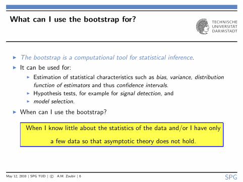
What can I use the bootstrap for?
◮ The bootstrap is a computational tool for statistical inference.
◮ It can be used for:
◮ Estimation of statistical characteristics such as bias, variance, distribution
function of estimators and thus confidence intervals.◮ Hypothesis tests, for example for signal detection, and◮ model selection.
◮ When can I use the bootstrap?
When I know little about the statistics of the data and/or I have only
a few data so that asymptotic theory does not hold.
May 12, 2010 | SPG TUD | c© A.M. Zoubir | 6 SPG
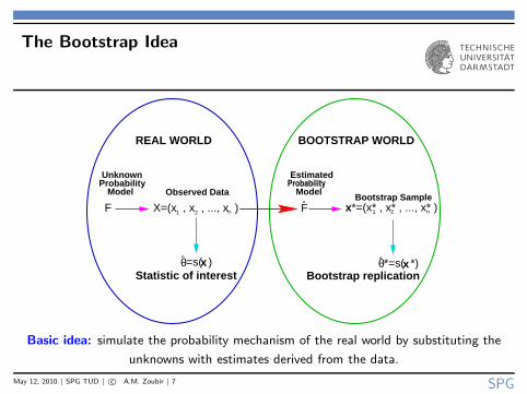
The Bootstrap Idea
Model
Unknown EstimatedProbability
Model
^
REAL WORLD
21X=(x , x , ..., x )F
Probability
θ
n
^
F^ x*=(x* , x* , ..., x* )1 2
θ*=s( *)x
Observed Data Bootstrap Sample
x=s( )Bootstrap replicationStatistic of interest
BOOTSTRAP WORLD
n
Basic idea: simulate the probability mechanism of the real world by substituting the
unknowns with estimates derived from the data.
May 12, 2010 | SPG TUD | c© A.M. Zoubir | 7 SPG
A Brief History Recount
◮ It was by marrying the power of Monte Carlo approximation with an
exceptionally broad view of the sort of problem that bootstrap methods
might solve, that [Efron (1979)] famously vaulted earlier resampling ideas out
of the arena of sampling methods and into the realm of a universal statistical
methodology.
◮ Arguably, the prehistory of the bootstrap encompasses pre-1979
developments of Monte Carlo methods for sampling.
◮ Important aspects of bootstrap roots lie in methods for spatial sampling in
India in the 1920’s [Hubback (1946), Mahalanobis (1946)], even before
Quenouille’s and Tukey’s work on the jackknife [Quenouille (1949, 1956),
Tukey (1958)].
May 12, 2010 | SPG TUD | c© A.M. Zoubir | 8 SPG
The independent data bootstrap
May 12, 2010 | SPG TUD | c© A.M. Zoubir | 9 SPG
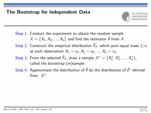
The Bootstrap for independent Data
Step 1. Conduct the experiment to obtain the random sample
X = {X1, X2, ... , Xn} and find the estimator θ from X .
Step 2. Construct the empirical distribution Fθ, which puts equal mass 1/n
at each observation X1 = x1, X2 = x2, ... , Xn = xn.
Step 3. From the selected Fθ, draw a sample X ∗ = {X ∗
1 , X ∗
2 , ... , X ∗
n },called the bootstrap (re)sample.
Step 4. Approximate the distribution of θ by the distribution of θ∗ derived
from X ∗.
May 12, 2010 | SPG TUD | c© A.M. Zoubir | 10 SPG
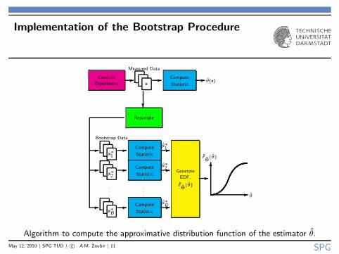
Implementation of the Bootstrap Procedure
Measured Data
Conduct
Experiment- - Compute
Statistic-
xθ(x)
?Resample
Bootstrap Data
- - Compute
Statistic-
x∗1
θ∗1
- - Compute
Statistic-
x∗2
θ∗2
.
.
.
.
.
.
- - Compute
Statistic-
x∗B
θ∗B
Generate
EDF,
FΘ
(θ)
-
-θ
6FΘ
(θ)
Algorithm to compute the approximative distribution function of the estimator θ.
May 12, 2010 | SPG TUD | c© A.M. Zoubir | 11 SPG
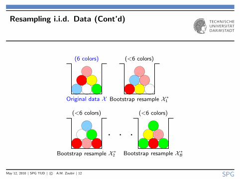
Resampling i.i.d. Data (Cont’d)
(6 colors) (<6 colors)
(<6 colors) (<6 colors)
Original data X Bootstrap resample X ∗
1
Bootstrap resample X ∗
2 Bootstrap resample X ∗
B
. . .
May 12, 2010 | SPG TUD | c© A.M. Zoubir | 12 SPG
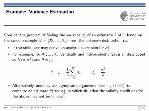
Example: Variance Estimation
Consider the problem of finding the variance σ2θ
of an estimator θ of θ, based on
the random sample X = {X1, ... , Xn} from the unknown distribution Fθ.
◮ If tractable, one may derive an analytic expression for σ2θ.
◮ For example, for X1, ... , Xn identically and independently Gaussian distributed
as N (µ, σ2) and θ = µ,
θ = µ =1
n
n∑
i=1
Xi , σ2µ =
σ2
n.
◮ Alternatively, one may use asymptotic arguments [Serfling (1980)] to
compute an estimate σ2θ
for σ2θ, in which situation the validity conditions for
the above may not be fulfilled.
May 12, 2010 | SPG TUD | c© A.M. Zoubir | 13 SPG

Example: Variance Estimation of µ
X = {X1, ... , Xn}
X ∗
1 X ∗
2 X ∗
B
µ∗
1 µ∗
2 µ∗
B
σ∗2µ = 1
B−1
∑B
b=1
(
µ∗
b − 1B
∑B
b=1 µ∗
b
)2
Observations
Resamples
Bootstrap statistics
Variance estimation
May 12, 2010 | SPG TUD | c© A.M. Zoubir | 14 SPG
The dependent data bootstrap
May 12, 2010 | SPG TUD | c© A.M. Zoubir | 15 SPG
The Dependent Data Bootstrap
◮ If a model such as AR is available for the probability mechanism generating
stationary observations, one could bootstrap independent residuals.
◮ If no plausible model exists, then one can resort to dependent data bootstrap
methodologies.
◮ Strong mixing processes, i.e., loosely speaking, processes for which
observations far apart (in time) are almost independent [Rosenblatt (1985)],
for example, satisfy the weak dependence condition.
◮ The moving blocks bootstrap [Kunsch (1989), Liu & Singh (1992), Politis &
Romano (1992,1994)] has been proposed for bootstrapping weakly dependent
data.
May 12, 2010 | SPG TUD | c© A.M. Zoubir | 16 SPG
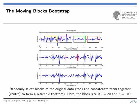
The Moving Blocks Bootstrap
0 10 20 30 40 50 60 70 80 90 100−5
0
5
Sample number
Am
plit
ud
e
Bootstrap Data0 10 20 30 40 50 60 70 80 90 100
−5
0
5
Am
plit
ud
e
Resampled Blocks
54321
0 10 20 30 40 50 60 70 80 90 100−5
0
5
Am
plit
ud
e
Observed Data
12 345
Randomly select blocks of the original data (top) and concatenate them together
(centre) to form a resample (bottom). Here, the block size is l = 20 and n = 100.
May 12, 2010 | SPG TUD | c© A.M. Zoubir | 17 SPG
Signal detection with the bootstrap
May 12, 2010 | SPG TUD | c© A.M. Zoubir | 18 SPG
Hypothesis Testing with the Bootstrap
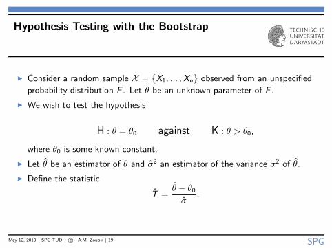
◮ Consider a random sample X = {X1, ... , Xn} observed from an unspecified
probability distribution F . Let θ be an unknown parameter of F .
◮ We wish to test the hypothesis
H : θ = θ0 against K : θ > θ0,
where θ0 is some known constant.
◮ Let θ be an estimator of θ and σ2 an estimator of the variance σ2 of θ.
◮ Define the statistic
T =θ − θ0
σ.
May 12, 2010 | SPG TUD | c© A.M. Zoubir | 19 SPG
Hypothesis Testing (Cont’d)
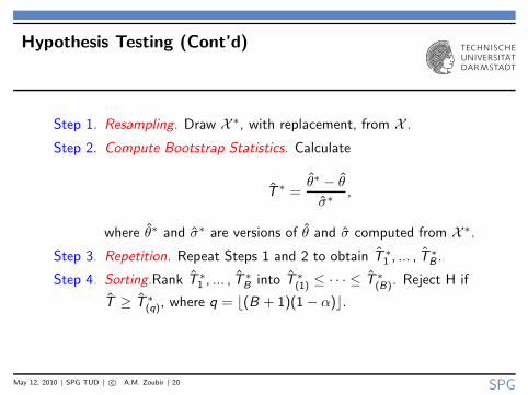
Step 1. Resampling. Draw X ∗, with replacement, from X .
Step 2. Compute Bootstrap Statistics. Calculate
T ∗ =θ∗ − θ
σ∗,
where θ∗ and σ∗ are versions of θ and σ computed from X ∗.
Step 3. Repetition. Repeat Steps 1 and 2 to obtain T ∗
1 , ... , T ∗
B .
Step 4. Sorting.Rank T ∗
1 , ... , T ∗
B into T ∗
(1) ≤ · · · ≤ T ∗
(B). Reject H if
T ≥ T ∗
(q), where q = ⌊(B + 1)(1 − α)⌋.
May 12, 2010 | SPG TUD | c© A.M. Zoubir | 20 SPG
Hypothesis Testing: Variance Estimation
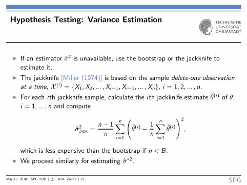
◮ If an estimator σ2 is unavailable, use the bootstrap or the jackknife to
estimate it.
◮ The jackknife [Miller (1974)] is based on the sample delete-one observation
at a time, X (i) = {X1, X2, ... , Xi−1, Xi+1, ... , Xn}, i = 1, 2, ... , n.
◮ For each ith jackknife sample, calculate the ith jackknife estimate θ(i) of θ,
i = 1, ... , n and compute
σ2JACK =
n − 1
n
n∑
i=1
(
θ(i) − 1
n
n∑
i=1
θ(i)
)2
,
which is less expensive than the bootstrap if n < B.
◮ We proceed similarly for estimating σ∗2.
May 12, 2010 | SPG TUD | c© A.M. Zoubir | 21 SPG
The Bootstrap Procedure
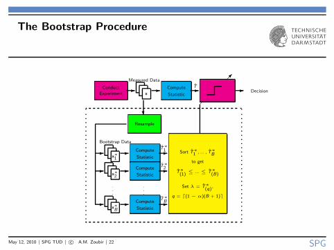
Measured Data
Conduct
Experiment- - Compute
Statistic-
x
T
?Resample
Bootstrap Data
- - Compute
Statistic-
x∗1
T∗1
- - Compute
Statistic-
x∗2
T∗2
.
.
.
.
.
.
- - Compute
Statistic-
x∗B
T∗B
Sort T∗1 , ... , T∗
B
to get
T∗(1)
≤ ... ≤ T∗(B)
Set λ = T∗(q)
,
q = ⌈(1 − α)(B + 1)⌉
Decision-�
May 12, 2010 | SPG TUD | c© A.M. Zoubir | 22 SPG
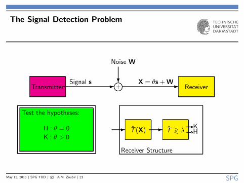
The Signal Detection Problem
+Transmitter Receiver- -?Signal s
Noise W
X = θs + W
Test the hypotheses:
H : θ = 0
K : θ > 0
Receiver Structure
T (X) T ≷ λ- - KH
May 12, 2010 | SPG TUD | c© A.M. Zoubir | 23 SPG
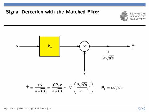
Signal Detection with the Matched Filter
Ps-x ×- T
1
σ√
s′s6
s
- -
T =s′x
σ√
s′s=
s′Psx
σ√
s′s∼ N
(
θ√
s′s
σ, 1
)
, Ps = ss′/s′s.
May 12, 2010 | SPG TUD | c© A.M. Zoubir | 24 SPG
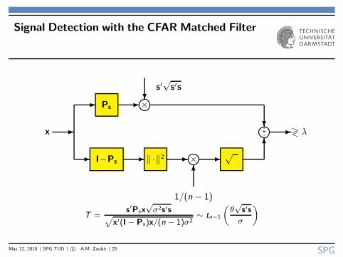
Signal Detection with the CFAR Matched Filter
×
·
·
Ps-
x
- ?
I−Ps ‖·‖2
×
-
6
s′√
s′s
-
- - - √6
? -
1/(n − 1)
≷ λ
T =s′Psx
√σ2s′s
p
x′(I − Ps)x/(n − 1)σ2∼ tn−1
„
θ√
s′s
σ
«
May 12, 2010 | SPG TUD | c© A.M. Zoubir | 25 SPG
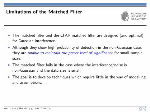
Limitations of the Matched Filter
◮ The matched filter and the CFAR matched filter are designed (and optimal)
for Gaussian interference.
◮ Although they show high probability of detection in the non-Gaussian case,
they are unable to maintain the preset level of significance for small sample
sizes.
◮ The matched filter fails in the case where the interference/noise is
non-Gaussian and the data size is small.
◮ The goal is to develop techniques which require little in the way of modelling
and assumptions.
May 12, 2010 | SPG TUD | c© A.M. Zoubir | 26 SPG
The Bootstrap in Signal Detection: Motivation
◮ The Bootstrap can provide solutions for detecting signals in non-Gaussian
interference, e.g., high-resolution radar and radar at low grazing angles.
◮ The bootstrap is particularly attractive when only a limited number of
samples is available for signal detection.
◮ The bootstrap is also attractive when detection is associated with estimation,
e.g., estimation of the number of signals.
◮ The bootstrap has been successfully applied to signal detection in areas such
as wireless communications, landmine detection, radar, sonar and biomedical
engineering.
May 12, 2010 | SPG TUD | c© A.M. Zoubir | 27 SPG

The Signal Detection Problem
+Transmitter Receiver- -?Signal s
Noise W
X = θs + W
Test the hypotheses:
H : θ = 0
K : θ > 0
Receiver Structure
T (X) T ≷ λ- - KH
May 12, 2010 | SPG TUD | c© A.M. Zoubir | 28 SPG
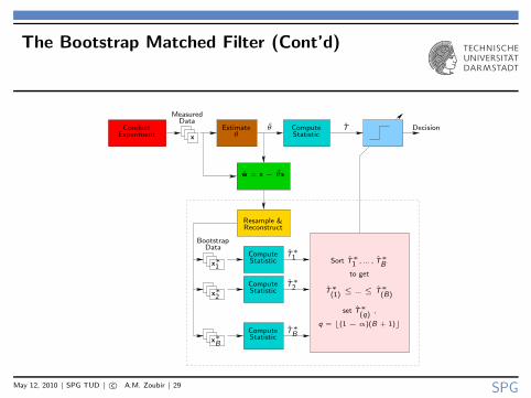
The Bootstrap Matched Filter (Cont’d)
ComputeStatistic
ComputeStatistic
ComputeStatistic
DataMeasured
x
Decision
Resample &
BootstrapData
ComputeStatistic
Estimateθ
Reconstruct
θ
T∗1
T∗2
T∗B
Sort T∗1 , ... , T∗
B
to get
T∗(1)
≤ ... ≤ T∗(B)
q = ⌊(1 − α)(B + 1)⌋
set T∗(q)
,
T
w = x − θs
ConductExperiment
x∗B
x∗2
x∗1
May 12, 2010 | SPG TUD | c© A.M. Zoubir | 29 SPG
Performance of the Bootstrap Matched Filter
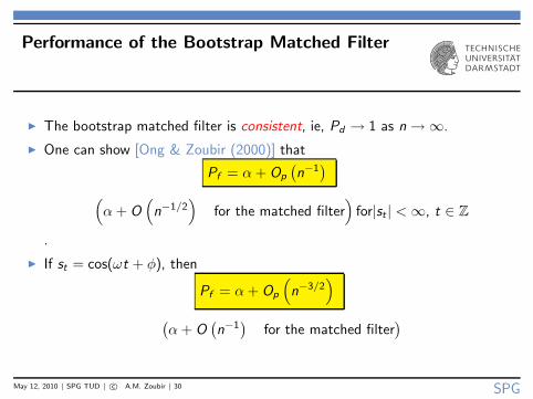
◮ The bootstrap matched filter is consistent, ie, Pd → 1 as n → ∞.
◮ One can show [Ong & Zoubir (2000)] that
Pf = α + Op
(
n−1)
(
α + O(
n−1/2)
for the matched filter)
for|st | < ∞, t ∈ Z
.
◮ If st = cos(ωt + φ), then
Pf = α + Op
(
n−3/2)
(
α + O(
n−1)
for the matched filter)
May 12, 2010 | SPG TUD | c© A.M. Zoubir | 30 SPG
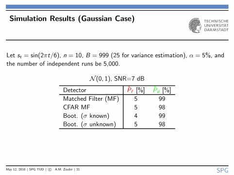
Simulation Results (Gaussian Case)
Let st = sin(2πt/6), n = 10, B = 999 (25 for variance estimation), α = 5%, and
the number of independent runs be 5,000.
N (0, 1), SNR=7 dB
Detector Pf [%] Pd [%]
Matched Filter (MF) 5 99
CFAR MF 5 98
Boot. (σ known) 4 99
Boot. (σ unknown) 5 98
May 12, 2010 | SPG TUD | c© A.M. Zoubir | 31 SPG
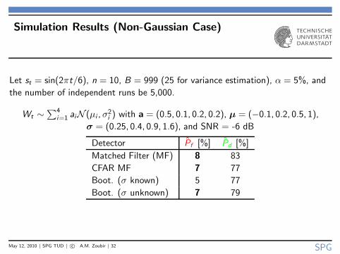
Simulation Results (Non-Gaussian Case)
Let st = sin(2πt/6), n = 10, B = 999 (25 for variance estimation), α = 5%, and
the number of independent runs be 5,000.
Wt ∼∑4
i=1 aiN (µi , σ2i ) with a = (0.5, 0.1, 0.2, 0.2), µ = (−0.1, 0.2, 0.5, 1),
σ = (0.25, 0.4, 0.9, 1.6), and SNR = -6 dB
Detector Pf [%] Pd [%]
Matched Filter (MF) 8 83
CFAR MF 7 77
Boot. (σ known) 5 77
Boot. (σ unknown) 7 79
May 12, 2010 | SPG TUD | c© A.M. Zoubir | 32 SPG
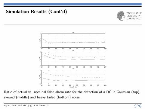
Simulation Results (Cont’d)
10 20 30 40 50 60 70 80 90 1000
1
2
3(a)
Pfa
/ α
10 20 30 40 50 60 70 80 90 1000
1
2
3(b)
Pfa
/ α
10 20 30 40 50 60 70 80 90 1000
1
2
3(c)
Pfa
/ α
Sample size
Ratio of actual vs. nominal false alarm rate for the detection of a DC in Gaussian (top),
skewed (middle) and heavy tailed (bottom) noise.
May 12, 2010 | SPG TUD | c© A.M. Zoubir | 33 SPG
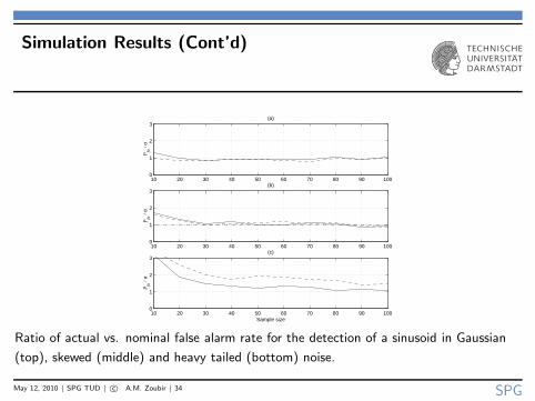
Simulation Results (Cont’d)
10 20 30 40 50 60 70 80 90 1000
1
2
3(a)
Pfa
/ α
10 20 30 40 50 60 70 80 90 1000
1
2
3(c)
Pfa
/ α
Sample size
10 20 30 40 50 60 70 80 90 1000
1
2
3
Pfa
/ α
(b)
Ratio of actual vs. nominal false alarm rate for the detection of a sinusoid in Gaussian
(top), skewed (middle) and heavy tailed (bottom) noise.
May 12, 2010 | SPG TUD | c© A.M. Zoubir | 34 SPG
Frequency domain bootstrap
methods for dependent data
May 12, 2010 | SPG TUD | c© A.M. Zoubir | 35 SPG
Bootstrapping Spectral Densities
◮ Confidence interval estimation (or hypothesis testing) for spectral densities is
encountered in numerous real-life applications, e.g., car engine monitoring.
◮ Two approaches to bootstrapping spectral densities:
◮ Use a time domain approach (block bootstrap) to bootstrap time series and
estimate bootstrap spectral density estimates from the time series replicae, or◮ use a technique that applies directly in the frequency domain.
◮ Bootstrap time series not always mimic the (complicated) dependence
structure of the underlying process.
◮ Frequency domain bootstrap methods do not require to first generate time
series replicae to get periodogram resamples.
May 12, 2010 | SPG TUD | c© A.M. Zoubir | 36 SPG
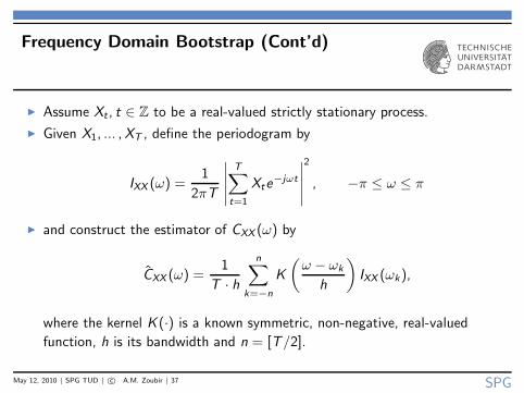
Frequency Domain Bootstrap (Cont’d)
◮ Assume Xt , t ∈ Z to be a real-valued strictly stationary process.
◮ Given X1, ... , XT , define the periodogram by
IXX (ω) =1
2πT
∣
∣
∣
∣
∣
T∑
t=1
Xte−jωt
∣
∣
∣
∣
∣
2
, −π ≤ ω ≤ π
◮ and construct the estimator of CXX (ω) by
CXX (ω) =1
T · h
n∑
k=−n
K
(
ω − ωk
h
)
IXX (ωk),
where the kernel K (·) is a known symmetric, non-negative, real-valued
function, h is its bandwidth and n = [T/2].
May 12, 2010 | SPG TUD | c© A.M. Zoubir | 37 SPG
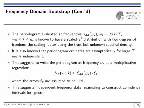
Frequency Domain Bootstrap (Cont’d)
◮ The periodogram evaluated at frequencies, IXX (ωk), ωk = 2πk/T ,
−n ≤ k ≤ n, is known to have a scaled χ2 distribution with two degrees of
freedom; the scaling factor being the true, but unknown spectral density.
◮ It is also known that periodogram ordinates are asymptotically for large T
nearly independent.
◮ This suggests to write the periodogram at frequency ωk as a multiplicative
regression:
IXX (ω : k) ≈ CXX (ωk) · Ek
where the errors Ek are assumed to be i.i.d.
◮ This suggests independent frequency data resampling to construct confidence
intervals for spectra.
May 12, 2010 | SPG TUD | c© A.M. Zoubir | 38 SPG
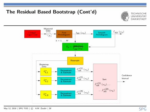
The Residual Based Bootstrap (Cont’d)
DataMeasured
x
ConductExperiment
BootstrapData
Reconstruct& Estimate
Reconstruct& Estimate
CXX
`
ωk
´
SmoothPeriodogram
Reconstruct& Estimate
Resample
Uk =IXX
`
ωk
´
CXX
`
ωk
´
Confidence
IntervalSort
k = 1, ... , M
FindPeriodogram
C∗(B)XX
`
ωk
´
C∗(2)XX
`
ωk
´
C∗(1)XX
`
ωk
´
, ...
... , C∗(B)XX
`
ωk
´
IXX
`
ωk
´
U∗k,1
U∗k,2
U∗k,B
C∗(1)XX
`
ωk
´
May 12, 2010 | SPG TUD | c© A.M. Zoubir | 39 SPG
Two real-life example
of the bootstrap
May 12, 2010 | SPG TUD | c© A.M. Zoubir | 40 SPG

Confidence Intervals for knock Spectra
◮ Special interest continues to a be reduction of fuel consumption in
combustion engines due to meeting the demands of new legislations on
greenhouse emission.
◮ A means for lowering fuel consumption in spark ignition engines is to increase
the compression ratio. Further increase in compression is limited by the
occurrence of knock.
◮ To attain safe operation at maximum efficiency, engine control systems which
detect knock and adapt spark timing of each cylinder separately have found
special interest.
◮ The data was collected at Robert Bosch GmbH on an engine test bed.
Measurements from a combustion engine running at 3500 rpm under
knocking conditions were recorded and sampled at 100 kHz.
May 12, 2010 | SPG TUD | c© A.M. Zoubir | 41 SPG
Confidence Intervals for knock Spectra
(Cont’d)
0 50 100 150 200 250 300 350 400−1
−0.8
−0.6
−0.4
−0.2
0
0.2
0.4
0.6
0.8
1
Sample
Am
plitu
de (
norm
alis
ed)
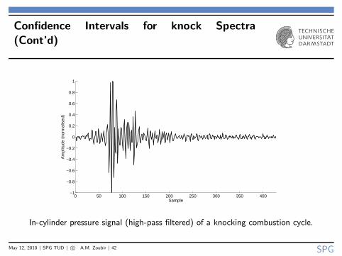
In-cylinder pressure signal (high-pass filtered) of a knocking combustion cycle.
May 12, 2010 | SPG TUD | c© A.M. Zoubir | 42 SPG
Confidence Intervals for knock Spectra
(Cont’d)
0 50 100 150 200 250 300 350 400−1
−0.8
−0.6
−0.4
−0.2
0
0.2
0.4
0.6
0.8
1
Sample
Am
plitu
de (
norm
alis
ed)
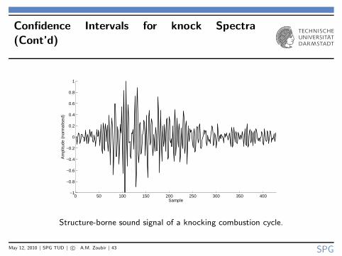
Structure-borne sound signal of a knocking combustion cycle.
May 12, 2010 | SPG TUD | c© A.M. Zoubir | 43 SPG

Confidence Intervals for knock Spectra
(Cont’d)
0 5 10 15 20 25 30 35 40 45 50−60
−50
−40
−30
−20
−10
0
Frequency [kHz]
Spe
ctra
l den
sity
(no
rmal
ised
)[dB
]
Spectral density estimates for in-cylinder pressure (solid —) and structure-borne sound
(dashed-dotted -.-) obtained by averaging 594 periodograms.
May 12, 2010 | SPG TUD | c© A.M. Zoubir | 44 SPG
Confidence Intervals for knock Spectra
(Cont’d)
0 5 10 15 20 25 30 35 40 45 50−50
−45
−40
−35
−30
−25
−20
−15
−10
−5
0
Frequency [kHz]
Spe
ctra
l den
sity
(no
rmal
ised
) [d
B]
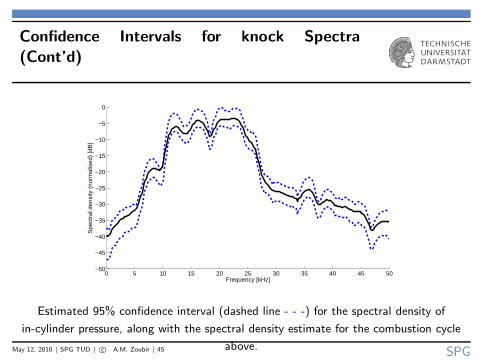
Estimated 95% confidence interval (dashed line - - -) for the spectral density of
in-cylinder pressure, along with the spectral density estimate for the combustion cycle
above.May 12, 2010 | SPG TUD | c© A.M. Zoubir | 45 SPG

Confidence Intervals for Knock Spectra
(Cont’d)
0 5 10 15 20 25 30 35 40 45 50−70
−60
−50
−40
−30
−20
−10
0
Frequency [kHz]
Spe
ctra
l den
sity
(no
rmal
ised
) [d
B]
Estimated 95% confidence interval for the spectral density of structure-borne sound
(dashed line - –), along with the spectral density estimate for the combustion cycle above
May 12, 2010 | SPG TUD | c© A.M. Zoubir | 46 SPG
Micro-Doppler Analysis
◮ Doppler often arises in engineering applications due to the relative motion of
an object with respect to the measurement system.
◮ If the motion is harmonic, for example due to vibration or rotation, the
resulting signal can be well modeled by an FM process [Huang et al. (1990)].
◮ Estimation of the FM parameters may allow one to determine physical
properties such as the angular velocity and displacement of the
vibrational/rotational motion which can in turn be used for classification.
Objective: Estimate the FM parameters along with a measure of accuracy,
such as confidence intervals.
May 12, 2010 | SPG TUD | c© A.M. Zoubir | 47 SPG
Micro-Doppler Analysis (Cont’d)
◮ Assume the following AM-FM signal model:
s(t) = a(t) exp{jϕ(t)}where a(t; α) =
∑q
k=0 αk tk and α = (α0, ... , αq) .
◮ The phase modulation for a micro-Doppler signal is described by:
ϕ(t) = −D/ωm cos(ωmt + φ) and the instantaneous frequency (IF) by:
ωi (t; β) ,dϕ(t)
dt= D sin(ωmt + φ),
where β = (D, ωm, φ) are the FM or micro-Doppler parameters.
◮ Given {x(k)}nk=1 of X (t) = s(t) + V (t), the goal is to estimate
β = (D, ωm, φ) as well as their confidence intervals.
May 12, 2010 | SPG TUD | c© A.M. Zoubir | 48 SPG
Micro-Doppler Analysis (Cont’d)
◮ The estimation of the phase parameters is performed using a time-frequency
Hough transform (TFHT) [Barbarossa & Lemoine (1996), Cirillo, Zoubir &
Amin (2006)].
◮ Once the phase parameters have been estimated, the phase term is
demodulated and the amplitude parameters are estimated via least-squares.
◮ Given estimates for α and β, the residuals are obtained.
◮ We whiten the residuals using a fitted AR model. The innovations are
re-sampled, filtered and added to the estimated signal term.
May 12, 2010 | SPG TUD | c© A.M. Zoubir | 49 SPG
Micro-Doppler Analysis (Cont’d)
◮ The results shown here are based on an experimental radar system*,
operating at carrier frequency fc = 919.82 MHz.
◮ After demodulation, the in-phase and quadrature baseband channels are
sampled at fs = 1 kHz.
◮ The radar system is directed toward a spherical object, swinging with a
pendulum motion, which results in a typical micro-Doppler signature.
◮ The PWVD of the observations is computed and shown below:
* Courtesy of Prof. Moeness Amin, Director of the Center of Advanced
Communications, Villanova University, Philadelphia, USA
May 12, 2010 | SPG TUD | c© A.M. Zoubir | 50 SPG
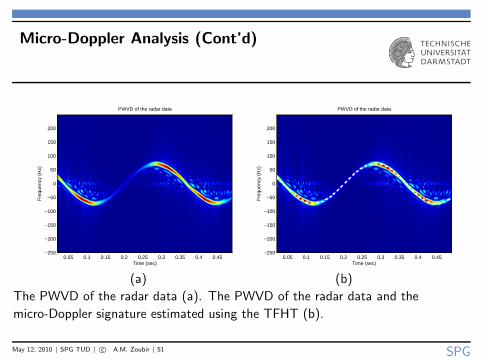
Micro-Doppler Analysis (Cont’d)
Time (sec)
Fre
quen
cy (
Hz)
PWVD of the radar data
0.05 0.1 0.15 0.2 0.25 0.3 0.35 0.4 0.45−250
−200
−150
−100
−50
0
50
100
150
200
Time (sec)F
requ
ency
(H
z)
PWVD of the radar data
0.05 0.1 0.15 0.2 0.25 0.3 0.35 0.4 0.45−250
−200
−150
−100
−50
0
50
100
150
200
(a) (b)
The PWVD of the radar data (a). The PWVD of the radar data and the
micro-Doppler signature estimated using the TFHT (b).
May 12, 2010 | SPG TUD | c© A.M. Zoubir | 51 SPG
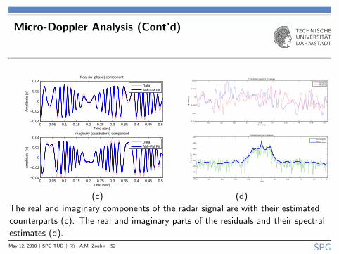
Micro-Doppler Analysis (Cont’d)
0 0.05 0.1 0.15 0.2 0.25 0.3 0.35 0.4 0.45 0.5−0.04
−0.02
0
0.02
0.04
Time (sec)
Am
plitu
de (
V)
Real (in−phase) component
DataAM−FM Fit
0 0.05 0.1 0.15 0.2 0.25 0.3 0.35 0.4 0.45 0.5−0.04
−0.02
0
0.02
0.04
Time (sec)
Am
plitu
de (
V)
Imaginary (quadrature) component
DataAM−FM Fit
0 0.05 0.1 0.15 0.2 0.25 0.3 0.35 0.4 0.45 0.5−0.015
−0.01
−0.005
0
0.005
0.01
Time (sec)
Am
plitu
de (
V)
Time−domain waveform of residuals
Re{ r(n) }Im{ r(n) }
−500 −400 −300 −200 −100 0 100 200 300 400 500−90
−80
−70
−60
−50
−40
−30
−20
f (Hz)
Pow
er (
dBW
)
Estimated spectrum of residuals
PeriodogramAR Fit
(c) (d)
The real and imaginary components of the radar signal are with their estimated
counterparts (c). The real and imaginary parts of the residuals and their spectral
estimates (d).May 12, 2010 | SPG TUD | c© A.M. Zoubir | 52 SPG
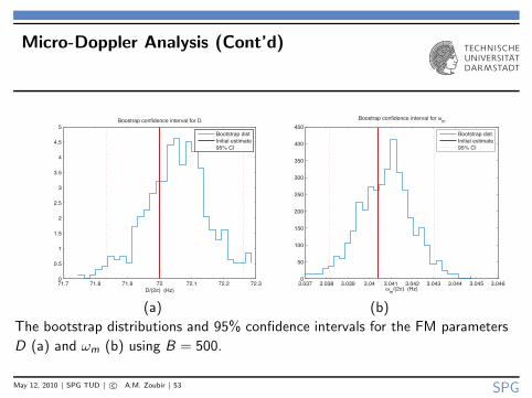
Micro-Doppler Analysis (Cont’d)
71.7 71.8 71.9 72 72.1 72.2 72.30
0.5
1
1.5
2
2.5
3
3.5
4
4.5
5
D/(2π) (Hz)
Boostrap confidence interval for D
.Bootstrap dist
Initial estimat
95% CI
e
3.037 3.038 3.039 3.04 3.041 3.042 3.043 3.044 3.045 3.0460
50
100
150
200
250
300
350
400
450
ωm
/(2π) (Hz)
Boostrap confidence interval for ωm
Bootstrap dist.
Initial estimate
95% CI
(a) (b)
The bootstrap distributions and 95% confidence intervals for the FM parameters
D (a) and ωm (b) using B = 500.
May 12, 2010 | SPG TUD | c© A.M. Zoubir | 53 SPG
Summary
◮ Many signal processing problems require the computation of quality measures
for estimators.
◮ Most techniques available assume that the size of the available set of sample
values is sufficiently large, so that “asymptotic” results can be applied.
◮ In many signal processing problems this assumption cannot be made because,
for example, the process is non-stationary and only small portions of
stationary data are considered.
◮ Bootstrap techniques are an alternative to asymptotic methods and provide
good results for many practical problems.
May 12, 2010 | SPG TUD | c© A.M. Zoubir | 54 SPG
Summary (Cont’d)
What was not discussed in this presentation:
◮ Other variants of the bootstrap such as bootstrap bagging and bootstrap
bumping [Tibshirani & Knight (1997)].
◮ Model selection with the bootstrap [Shao & Tu (1995), Zoubir (1999)].
◮ Hypothesis testing [Hall & Titterington (1989), Hall & Wilson (1991), Hall
(1992)] and signal detection [Zoubir (2000)].
◮ Bayesian approaches to the bootstrap.
May 12, 2010 | SPG TUD | c© A.M. Zoubir | 55 SPG

Which Method Should I Use?
May 12, 2010 | SPG TUD | c© A.M. Zoubir | 56 SPG

The Baron von Munchhausen
Varney, Allen (2007), ”The Extraordinary Adventures of Baron Munchhausen”, in Lowder, James, Hobby Games: The Best 100, Green Ronin Publishing,
pp. 107109, ISBN 978-1-932442-96-0
May 12, 2010 | SPG TUD | c© A.M. Zoubir | 57 SPG