HAL Id: hal-00493860https://hal.archives-ouvertes.fr/hal-00493860

Submitted on 8 Nov 2010

HAL is a multi-disciplinary open accessarchive for the deposit and dissemination of sci-entific research documents, whether they are pub-lished or not. The documents may come fromteaching and research institutions in France orabroad, or from public or private research centers.

L’archive ouverte pluridisciplinaire HAL, estdestinée au dépôt et à la diffusion de documentsscientifiques de niveau recherche, publiés ou non,émanant des établissements d’enseignement et derecherche français ou étrangers, des laboratoirespublics ou privés.

The Blasius equationAugustin Fruchard, Bernard Brighi, Tewfik Sari

To cite this version:

Augustin Fruchard, Bernard Brighi, Tewfik Sari. The Blasius equation. 2010. <hal-00493860>

The Blasius equation

Bernard Brighi, Augustin Fruchard and Tewfik Sari

June 14, 2010

Abstract. The Blasius problem f ′′′ + ff ′′ = 0, f(0) = −a, f ′(0) = b,f ′(+∞) = λ is investigated, in particular in the difficult and scarcely stud-ied case b < 0 6 λ. The shape and the number of solutions are determined.The method is first to reduce to the Crocco equation uu′′ + s = 0 and then touse an associated autonomous planar vector field. The most useful propertiesof Crocco solutions appear to be related to canard solutions of a slow fast vec-tor field.

Keywords : Blasius equation, Crocco equation, boundary value problem oninfinite interval, canard solution.

1 Introduction

This is the report of a talk given in Rencontre du reseau Georges Reeb a la

memoire d’Emmanuel Isambert, Paris, December 21 - 22, 2007.We present in this article a selection of results of [6]. The reader is referred

to [6] for complete proofs, additional and intermediate results. We take theoccasion to completely change the order of presentation: in [6] we first givethe results on the Blasius equation with a sketch of proof, then we introducethe Crocco equation and the vector field, we establish results and proofs onthese intermediate equations and then we return to the proof of the initialresult. Here we choose a different order and we postpone the main resultat the end of the article. We hope that this article may be a first approachbefore a thorough study of [6].

The paper is organized as follows. In Section 2, we state the main problemof the paper which is the investigation of the following Blasius BoundaryValue Problem (BBVP for short)

f ′′′ + ff ′′ = 0 on [0,+∞[, (1)

f(0) = −a, f ′(0) = b, limt→+∞

f ′(t) = λ. (2)

We list some former results, according to the relative values of b and λ, andwe focus our attention on the case b < 0 6 λ, which is our case of interest.In Section 3, we show that, in the latter case, this boundary value problemis equivalent to the Crocco Boundary Value Problem (CBVP)

uu′′ + s = 0 on [b, λ[,

u′(b) = a, lims→λ

u(s) = 0.(3)

where [b, λ[ appears as the maximal right-interval of definition of the solu-tion. In Section 4, we show that the similarity properties of the Blasius or

the Crocco solutions permit to reduce the non autonomous second order dif-ferential equation of Crocco to an autonomous planar vector and we noticethat the maximal right-interval of definition of the solutions of the Croccoequation presents a discontinuity with respect to the initial condition. Itis well known that the maximal right-interval of definition of the solutionof a differential equation is not continuous in general with respect to theinitial conditions. It is simply lower semicontinuous. Actually, in Section 6,we see that the solutions of the Crocco differential equation which are closeto 0 for s close to 0 are canard solutions of a slow-fast vector field. Thesesolutions play an important role in the description of the discontinuity of themaximal right-interval of definition of the solution of the Crocco equation.In Section 7, we analyze this discontinuity which occurs along a particularorbit of the planar vector field considered in Section 4. In Section 8, we givea lower bound of the number of solutions of the boundary value problemassociated to the Blasius equation, in the case b < 0 6 λ. In Section 9,we describe a difficulty encountered in numerical simulations. Indeed, dueto the canard solutions phenomenon, some solutions of the Crocco equationbecome exponentially small for s < 0 and the numerical scheme cannot givethe right solution. We show how to use the theoretical study in Section 5 toovercome this difficulty.

2 The Blasius Boundary Value Problem

The Blasius Boundary Value Problem (1-2) arises for the first time, witha = b = 0 and λ = 2, in 1907 in the thesis of Blasius [3, 4]. In the casea = b = 0, Hermann Weyl [16] proves that the BBVP has one and onlyone solution. The proof is very elementary but strongly uses the fact thata = b = 0, see also [5, 8]. The BBVP plays a central role in fluid mechanics[12]: The Blasius equation (1) was obtained using a similarity transform andenabled successful treatment of the laminar boundary layer on a flat plate.Since equation (1) can be seen as a first order linear differential equation forf ′′, we have

f ′′(t) = f ′′(0) exp

{

−∫ t

0

f(τ)dτ

}

.

Hence, the BBVP splits into three cases, called respectively linear, concaveand convex:

• If λ = b, then the BBVP has a unique solution, given by f(t) = bt − a.

• If λ > b, then any possible solution must satisfy f ′′(t) > 0 for all t > 0,i.e. has to be convexe.

• If λ < b, then possible solutions are concave.

The concave case is completely solved and well-known [1].

1

Proposition 1 — In the case λ < b, the BBVP (1 - 2) has exactly onesolution if 0 6 λ < b, and no solution if λ < 0.

When b > 0, the convex case λ > b is also well-known, see [8].

Proposition 2 ([6] Corollary 3.6) — The BBVP (1 - 2), where b > 0 andλ > b, has exactly one solution when a 6 0 or b > 0. When a > 0 andb = 0, the BBVP has exactly one solution for all λ > a2λ+ and no solutionif 0 < λ 6 a2λ+, where λ+ ≃ 1.304 is defined in Proposition 5.

We know that every solution of the Blasius equation (1) such that f ′′(0) > 0is defined for all t and its derivative has a finite and non-negative limit ast → +∞ ([6] Proposition 3.1). Thus

Proposition 3 — The BBVP (1 - 2) has no solution if b < λ < 0.

b

λ

a2λ+−

linear

linear

convex

concave

0

0

0

1

1

1

11

1

0

Figure 1: In the plane (b, λ), the number of solutions of the BBVP (5) ineach region and on their border. In gray, the remaining region to investigate,purpose of this article.

In this article, we focus on the remaining case b < 0 6 λ, which is much richerand trickier. Non uniqueness for the BBVP is mentioned in the literature,but either only supported by numerical investigations [9], or with incompleteproofs [10, 13].

The Blasius equation (1) has the following similarity property:

If t 7→ f(t) is a solution of (1), so is t 7→ σf(σt), for all σ ∈ R. (4)

This allows us to restrict our attention without loss of generality to the caseb = −1, i.e. to the BBVP

f ′′′ + ff ′′ = 0 on [0,+∞[,

f(0) = −a, f ′(0) = −1, limt→+∞

f ′(t) = λ > 0.(5)

The purpose of this article is to count the number of solutions of (5). Themain result, at the end of Section 8, gives a minimum number of solutions of(5) depending on the values of a and λ. We conjecture that this minimumnumber is the exact number of solutions.

3 The Crocco Boundary Value Problem

Since f ′′ > 0 it follows that t 7→ f ′(t) is a diffeomorphism. Hence we canuse f ′ as an independent variable and express f ′′ as a function of f ′. Thisis the so-called Crocco transformation [7]

s = f ′, f ′′ = u(s)

Differentiating f ′′ = u(f ′) we obtain u′(s) = −f . Differentiating once againwe obtain u′′(s)u(s) = −s. Thus the Blasius equation (1) is equivalent tothe Crocco differential equation

u′′u + s = 0 (6)

0

2

4

6

8

10

5 10

0

0.5

1

–1 1

Figure 2: On the left, the Blasius solution t 7→ f(t;−2, 1); on the right, thecorresponding Crocco solution s 7→ u(s;−2, 1).

As we will see, the BBVP (5) is equivalent to the Crocco Boundary ValueProblem (3) for b = −1, rewritten below for convenience

uu′′ + s = 0 on [−1, λ[,

u′(−1) = a, lims→λ

u(s) = 0.(7)

2

The equivalence between (5) and (7) will become clear after the followingremarks. In order to solve (5) we use the shooting method. Let f( · ; a, c)denote the solution of the Blasius Initial Value Problem (BIVP)

f ′′′ + ff ′′ = 0, f(0) = −a, f ′(0) = −1, f ′′(0) = c > 0. (8)

The solution f( · ; a, c) is defined for all t > 0 and its derivative has a finiteand non-negative limit as t → +∞ ([6] Proposition 3.1). Let £(a, c) denotethe limit1

£(a, c) := limt→+∞

f ′(t; a, c) > 0. (9)

Then ([6] Proposition 2.1), [−1,£(a, c)[ is the maximal right interval of ex-istence of the solution u( · ; a, c) of the Crocco Initial Value Problem (CIVP)

uu′′ + s = 0, u(−1) = c > 0, u′(−1) = a. (10)

See Figure 2 for a comparison between a Blasius solution and the corre-sponding Crocco solution.

Moreover, we have

lims→£(a,c)

u(s) = 0 and(

£(a, c) > 0 ⇒ lims→£(a,c)

u′(s) = −∞)

This shows that (5) is equivalent to (7).

4 Use of symmetries to reduce the order

The similarity property (4) is rewritten as follows for the Crocco equation(6)

If σ > 0 and s 7→ u(s) is a solution of (6), so is uσ : s 7→ σ3u(σ−2s). (11)

This similarity property reduces the Crocco equation (6) to a system ofautonomous differential equations. Actually, the change of variables

x(s) = (−s)−1/2u′ (s) , y(s) = (−s)−3/2u (s)

leads to the system

x′ =

12 x + 1

y

−s, y′ =

x + 32 y

−s.

Thus, using the change of independent variable s = −e−τ , we obtain theplanar vector field

x =1

2x +

1

y, y = x +

3

2y, (12)

1This function £ is denoted by eΛ in [6].

Γ∞

S∗

-x

6y

�y = R1(x)

xy = −2

@Iy = L1(x)

@Ry = R2(x)

Γ∞

S∗

-xa2 a3 a1

Figure 3: On the left: the phase portrait of (12). On the right: sketch ofenlargement of Γ∞ near S∗. The functions Ln and Rn are defined in Section7.

where the dot is for differentiating with respect to the new independentvariable τ . The initial conditions u(−1) = c, u′(−1) = a in the CIVP (10)correspond to

x(0) = a, y(0) = c.

Notice that this vector field describes the Crocco equation (6) only for s < 0,since τ tends to +∞ as s tends to 0.

Because the transformation u 7→ uσ given by (11) corresponds to the shiftτ 7→ τ + 2 ln σ, to each orbit

{(

x(τ), y(τ))

; τ ∈ R}

of a solution of (12)corresponds a whole family (uσ)σ>0 of solutions of (6) connected by thesimilarity (11). In particular, the unique stationary point S∗ =

(

−√

3, 2√3

)

of (12) corresponds to the unique self-similar positive solution u∗ of (6), i.e.

satisfying u∗(s) = σ3u∗(σ−2s) for s < 0 < σ, namely

u∗(s) = 2√3(−s)3/2. (13)

A study of this vector field, detailed in [6], shows the following.

• All solutions of (12) are defined on R and tend to S∗ as τ → −∞.

• There is one and only one orbit, denoted by Γ∞, such that any solution

(x, y) parametrizing Γ∞ satisfies that x(τ)y(τ) tends to −1 as τ → +∞, see

Figure 3.

• For all solutions(

x(τ), y(τ))

except those on Γ∞ ∪ {S∗}, the quotientx(τ)y(τ) tends to 0 as τ → +∞.

• ([6] Theorem 2.4) For all solutions(

x(τ), y(τ))

except those on Γ∞ ∪{S∗}, x(τ)3

y(τ) has a limit k ∈ R as τ → +∞. The number k parametrizes

3

the orbit of (12) denoted by Γk. In terms of positive Crocco solutions,we have the following properties:

1. if (a, c) ∈ Γ∞ then lims→0−

u(s; a, c) = 0 and lims→0−

u′(s; a, c) < 0,

2. if (a, c) = S∗ then lims→0−

u(s; a, c) = 0 and lims→0−

u′(s; a, c) = 0,

3. Otherwise (a, c) ∈ Γk for some k ∈ R. In that case, u(0; a, c) > 0and u′(0; a, c) is of the same sign as k.

Let (a, c) be an initial condition which is close to Γ∞. If (a, c) lies on

0.5

1

1.5

–1 –0.5

0.5

1

1.5

–1 –0.5 0.5 1 1.5 2

�1-

r(a; 1)r(a; 2)a

Daa2 a3 a1 -s

6ur 1

-s6ur 2

Figure 4: A sketch of the spiral Γ∞ and two numerical Crocco solutions withinitial conditions u1(−1) = c1 = 1.78, u′

1(−1) = a = −2 and u2(−1) = c2 =1.62, u′

2(−1) = a = −2, where (a, c1) and (a, c2) are on the convex and onthe concave sides of Γ∞ respectively.

the convex side of Γ∞, then u(0; a, c) is close to 0 and u′(0; a, c) < 0. Sinceu(s; a, c) becomes concave for s > 0, it follows that £(a, c) is close to 0. If(a, c) lies on the concave side of Γ∞, then u(0; a, c) is small and u′(0; a, c) > 0.Thus £(a, c) is not close to 0, see Figure 4. This shows that the function£(a, c) is discontinuous on Γ∞. The precise description of this discontinuityneeds the knowledge of the behavior of the solutions u(s) of the Croccoequation (6) for which u(0) is close to 0. This behavior is described in thefollowing section.

5 Crocco solutions near u = 0 ...

The following result describes Crocco solutions close to 0 and with positiveslope for s = 0: they take an exponentially small value at some small negativeabscissa of s and then go far from the s axis.

Proposition 4 — Fix α > 0 and let 0 < ε → 0. Let u = u(s, ε) denote thesolution of (6) such that u(0, ε) = ε and u′(0, ε) = α. Then u(s, ε) reaches

-− 1

α0 S

6

1

U

@@

@��

��

r

-−α 0 α V

6U

1 r

-−α 0 α V

6S

@I − 1α

r

0,4

-0,4

0,2

0-0,6-0,8-1

1

0

0,8

-0,2

0,6

210-1-2

2

0

210-1-20

Figure 5: Above: schematic graphs of the solution of (14) in the limit ε → 0,respectively in the variables S,U , the variables U, V and S, V . Below: thenumerical solution corresponding to ε = 0.1 and α = 2.

its minimum at some abscissa s = κ(ε) < 0 satisfying κ(ε) = − εα

(

1 + o(1))

and

u(κ(ε), ε) = exp(

− α3

2ε

(

1 + o(1))

)

as ε → 0.

Moreover, for all B < 0 fixed, we have u(εs, ε) = ε(

|αs+1|+o(1))

as ε → 0,uniformly for s ∈ [B, 0].

Proof. The reference [6] contains two proofs: one in Section 5 and analternative one in Section 6. We give here an overview of the second one.The solution u(s, ε) is defined for all s 6 0 and is positive. The functionU(S, ε), defined by

U(S, ε) =1

εu (εS, ε) ,

is the solution of the initial value problem

Ud2U

dS2+ εS = 0, U(0) = 1,

dU

dS(0) = α. (14)

Except near the axis U = 0, and for bounded values of S, U ′′ is close to 0, i.e.

the solutions are almost affine. Precisely, one has for all fixed S0 ∈]

− 1α , 0

]

U(S, ε) = αS + 1 + o(1) as ε → 0, uniformly for S ∈ [S0, 0] (15)

What is less obvious is that this approximation is still valid up to − 1α

and that, for any fixed B 6 − 1α , the solution satisfies the approximation

4

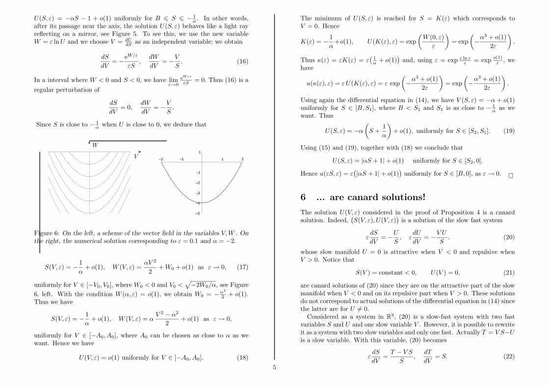
U(S, ε) = −αS − 1 + o(1) uniformly for B 6 S 6 − 1α . In other words,

after its passage near the axis, the solution U(S, ε) behaves like a light rayreflecting on a mirror, see Figure 5. To see this, we use the new variableW = ε ln U and we choose V = dU

dS as an independent variable; we obtain

dS

dV= −eW/ε

εS,

dW

dV= −V

S. (16)

In a interval where W < 0 and S < 0, we have limε→0

eW/ε

εS = 0. Thus (16) is a

regular perturbation of

dS

dV= 0,

dW

dV= −V

S.

Since S is close to − 1α when U is close to 0, we deduce that

–5

–4

–3

–2

–1

1

–2 –1 1 2

-V

6W

Figure 6: On the left, a scheme of the vector field in the variables V,W . Onthe right, the numerical solution corresponding to ε = 0.1 and α = −2.

S(V, ε) = − 1

α+ o(1), W (V, ε) =

αV 2

2+ W0 + o(1) as ε → 0, (17)

uniformly for V ∈ [−V0, V0], where W0 < 0 and V0 <√

−2W0/α, see Figure

6, left. With the condition W (α, ε) = o(1), we obtain W0 = −α3

2 + o(1).Thus we have

S(V, ε) = − 1

α+ o(1), W (V, ε) = α

V 2 − α2

2+ o(1) as ε → 0,

uniformly for V ∈ [−A0, A0], where A0 can be chosen as close to α as wewant. Hence we have

U(V, ε) = o(1) uniformly for V ∈ [−A0, A0]. (18)

The minimum of U(S, ε) is reached for S = K(ε) which corresponds toV = 0. Hence

K(ε) = − 1

α+o(1), U(K(ε), ε) = exp

(

W (0, ε)

ε

)

= exp

(

−α3 + o(1)

2ε

)

.

Thus κ(ε) = εK(ε) = ε(

1α + o(1)

)

and, using ε = exp ε ln εε = exp o(1)

ε , wehave

u(κ(ε), ε) = εU(K(ε), ε) = ε exp

(

−α3 + o(1)

2ε

)

= exp

(

−α3 + o(1)

2ε

)

.

Using again the differential equation in (14), we have V (S, ε) = −α + o(1)uniformly for S ∈ [B,S1], where B < S1 and S1 is as close to − 1

α as wewant. Thus

U(S, ε) = −α

(

S +1

α

)

+ o(1), uniformly for S ∈ [S2, S1]. (19)

Using (15) and (19), together with (18) we conclude that

U(S, ε) = |αS + 1| + o(1) uniformly for S ∈ [S2, 0].

Hence u(εS, ε) = ε(

|αS + 1| + o(1))

uniformly for S ∈ [B, 0], as ε → 0.

6 ... are canard solutions!

The solution U(V, ε) considered in the proof of Proposition 4 is a canardsolution. Indeed,

(

S(V, ε), U(V, ε))

is a solution of the slow fast system

εdS

dV= −U

S, ε

dU

dV= −V U

S. (20)

whose slow manifold U = 0 is attractive when V < 0 and repulsive whenV > 0. Notice that

S(V ) = constant < 0, U(V ) = 0, (21)

are canard solutions of (20) since they are on the attractive part of the slowmanifold when V < 0 and on its repulsive part when V > 0. These solutionsdo not correspond to actual solutions of the differential equation in (14) sincethe latter are for U 6= 0.

Considered as a system in R3, (20) is a slow-fast system with two fast

variables S and U and one slow variable V . However, it is possible to rewriteit as a system with two slow variables and only one fast. Actually T = V S−Uis a slow variable. With this variable, (20) becomes

εdS

dV=

T − V S

S,

dT

dV= S. (22)

5

6T

*S

jV

r(α,0,−1)

**s

**

@I(α,− 1

α,−1)

�(−α,− 1

α,1)

Figure 7: The canard of (22).

This is a singularly perturbed system whose slow manifold is the surfaceT = V S. This slow manifold is attractive for V < 0 and repulsive forV > 0. The Tikhonov theorem (see [14, 11] and [15] Section 39) describesthe behavior of the solution

(

S(V, ε), T (V, ε))

of (22) when V > 0. There is a

fast transition (see Figure 7) taking the trajectory(

V, S(V, ε), T (V, ε))

, from

its initial point (α, 0,−1), to a o(1) neighborhood of the point(

α,− 1α ,−1

)

of

the slow manifold, preceded by a slow transition near a solution(

− 1α ,−V

α

)

of the reduced problem

S =T

V,

dT

dV= S.

More precisely, for any A0 and A1, such that 0 < A1 < A0 < α, we have

S(V, ε) = − 1

α+ o(1) uniformly for V ∈ [A1, A0], (23)

T (V, ε) = −V

α+ o(1) uniformly for V ∈ [A1, α].

Notice that A0 (resp. A1) is fixed but may be chosen as close to α (resp. 0),as we want. The approximation for S does not hold near V = α since thereis a boundary layer (fast transition) from S = 0 at V = α to S = − 1

α for Vclose to α. We deduce that

U(V, ε) = V S(V, ε) − T (V, ε) = o(1), uniformly for V ∈ [A1, α]. (24)

A priori, Tikhonov theorem does not apply for V 6 0, because for V = 0the slow manifold becomes repulsive, but we will see that (24) still holdsfor negative values of V . This is the so-called bifurcation delay [2]. Theslow manifold is foliated by the explicit solutions S(V ) = S0 = constant,T (V ) = V S0, corresponding to the solutions (21). These solutions are canardsolutions since they follow the attractive part and then the repulsive partof the slow manifold, see Figure 7. Knowing the “exit” value V = α of the

solution T (V, ε) in a small neighborhood of the slow manifold, we want tocompute now the “entry” value for which the solution was far from the slowmanifold. Since U = V S − T > 0, we use the change of variable W = ε lnUwhich proves that the “entry” of the solution in the neighborhood of theslow manifold holds asymptotically for V = −α, as shown in the proof ofProposition 4. For details and complements see [6] Section 6.

7 The discontinuity of the function £

Two particular solutions of the Crocco equation (6) play an important rolein our study.

0.2

0.4

0.6

0.8

1

1.2

1.4

0–1 –0.8 –0.6 –0.4 –0.2

0

0.2

0.4

0.2 0.4 0.6 0.8 1 1.2 1.4

Figure 8: The graphs of u− on the left and of u+ on the right.

Proposition 5 ([6] Theorem 2.2) — The Crocco equation (6) has two so-lutions, denoted by u− and u+ such that u− is the unique solution of (6)satisfying

lims→0−

u−(s) = 0, lims→0−

u′−(s) = −1

and u+ is the unique solution of (6) satisfying

lims→0+

u+(s) = 0, lims→0+

u′+(s) = 1.

The solution u− is defined on ]− ∞, 0[ and the solution u+ is defined on]0, λ+[ for some λ+ > 0.

Numerical computations give λ+ ≈ 1.303918. See Figure 8 for the graphs ofu− and u+.

The orbit Γ∞ on which £ is discontinuous (See Figure 4 for an illustrationof this discontinuity) is given by

Γ∞ ={

m(s) =(

(−s)−1/2u′−(s), (−s)−3/2u−(s)

)

; s < 0}

.

A consequence of Proposition 4 is the following; see [6] Section 5.2 for theproofs.

6

Proposition 6 — For every sequence(

(αn, γn))

n∈Nwhich tends to m(−1),

the sequence(

u′(0;αn, γn))

n∈Nis bounded and has at most two cluster

points: 1 and −1. Precisely, if (αn, γn) tends to m(−1) on the convexside then u′(0;αn, γn) tends to −1, and if (αn, γn) tends to m(−1) on theconcave side then u′(0;αn, γn) tends to 1.

Remark — This statement seems to contradict the well-known property ofcontinuity with respect to initial conditions: if (a1, c1) and (a2, c2) are twopoints close to m(−1) such that u′(0; a1, c1) is close to −1 and u′(0; a2, c2)close to 1, then this continuity property seems to imply that, for any fixed d ∈]−1, 1[ there would exist (a, c) between (a1, c1) and (a2, c2) with u′(0; a, c) =d. In fact there is no contradiction: any small path joining (a1, c1) and(a2, c2) has to cross the “singular line”

{(

u−(s), u′−(s)

)

; s < 0}

at somepoint (a0, c0) and the solution with this initial condition is no longer definedat 0. This could explain an error in [13] Lemma 2 p. 257, which asserts thecontinuity of £.

8

2

6

0

4

2

-20

-4-6

1

0

-1

2

-2

-3

0-2-4-6

2

Figure 9: Numerical graphs of some orbits Γk and of the level set curves ofthe function £. On the left nine curves Γk for various values of k ∈ R∪{∞}and £(a, c) = λ for λ = 0, 1 and 10. On the right the sames curves in theplane (a, ln c), showing the details for small values of c. The flow of (12)transforms a level curve of £(a, c) into another level curve. Notice that thelevel set curve £(a, c) = 0 is equal to the orbit Γ∞.

Proposition 6 shows that the discontinuity of £ at the point m(−1) of Γ∞

is equal to λ+, see [6] Theorem 2.5. The discontinuity of £ at any pointm(s) of Γ∞ can be obtained using the similarity property (11). To see this,let Λ(a, b, c) denote the limit, when t → ∞, of the derivative f ′(t) of the

solution f(t) of the BIVP

f ′′′ + ff ′′ = 0, f(0) = −a, f ′(0) = b, f ′′(0) = c > 0.

This limit is finite and non negative ([6] Proposition 3.1). The function £ issimply given by

£(a, c) = Λ(a,−1, c).

Then ([6] Proposition 2.1), [−1,Λ(a, b, c)[ is the maximal right interval ofexistence of the solution u(s) of the CIVP

uu′′ + s = 0, u(b) = c > 0, u′(b) = a.

The similarity property (11) implies

∀σ > 0, Λ(σa, σ2b, σ3c) = σ2Λ(a, b, c). (25)

This formula justifies, as said in the introduction, that the properties of Λfor b < 0 can be deduced from the case b = −1, i.e. from the properties ofthe function £ : (a, c) 7→ Λ(a,−1, c).

Notice that, for any positive solution u of the Crocco equation defined onsome interval I, we have

∀s ∈ I, £(

u′(−1), u(−1))

= Λ(

u′(−1),−1, u(−1))

= Λ(

u′(s), s, u(s))

.

As a consequence, (25) gives

∀s < 0, £(

u′(−1), u(−1))

= −s£(

(−s)−1/2u′(s), (−s)−3/2u(s))

.

In terms of the associated vector field, we deduce that for all (x, y) solutionof (12)

∀τ ∈ R, £(

x(τ), y(τ))

= eτ£(

x(0), y(0))

. (26)

This formula shows how the τ -map flow of (12) transforms the level curve£(a, c) = λ into the level curve £(a, c) = eτλ, see Figure 9. Hence thesimilarity property (11) yields the discontinuity at any point of Γ∞.

Corollary 7 — The discontinuity of £ at a point m(s) of Γ∞ is as follows:on the convex side of Γ∞, £ tends to 0, whereas on the concave side, £ tendsto −λ+

s .

8 The number of solutions of the BBVP

To count the number of solutions of (5) we adopt the following strategy: forany values of a ∈ R and λ > 0, we count the number of values of c for which£(a, c) = λ where £ : R×]0,+∞[→ [0,+∞[ is the limit defined by (9). LetA(λ) denote the abscissa of the point of Γ∞ where £ takes the values 0 and

7

–3

–2

–1

01 2 3 4 5 6

–1.73

–1.725

–1.72

–1.715

0 0.02 0.04 0.06 0.08 0.1

−√

3a = A(λ)

λ

−√

3

a

λ

a = A(λ)

Figure 10: On the left: the graph of A. On the right: an enlargement near(0,−

√3).

λ on each side of Γ∞ respectively. Corollary 7 yields −s = λ+

λ , from whichwe deduce that

A : ]0,+∞[ → ]−∞, 0[ , λ 7→√

λλ+

u′−

(

−λ+

λ

)

.

See Figure 10 for a numerical graph of A and Figure 12 for a sketch showingthe oscillations near λ = 0. A careful study of the vector field shows thatΓ∞ has no inflexion point and S∗ is a focus. Therefore for all n > 1, withthe convention a0 = −∞, there exist functions

Ln : [a2n, a2n−1] → R, Rn : [a2n−2, a2n−1] → R,

Ln convex and Rn concave, such that Γ∞ is the union of the graphs of themappings x 7→ Ln(x) and x 7→ Rn(x); see Figure 3 right for the graphs of R1,R2 and L1. As a consequence, the function A has the following properties.

Proposition 8 ([6] Proposition 1.1) — The function A is C∞ and has aninfinite sequence of extremal points (λn)n>1 decreasing to 0: local minimaat λ2n and local maxima at λ2n+1, and no other extremum. Let A(λn) = an

denote these extremal values. Sequences (a2n) and (a2n+1) are adjacent and

limn→+∞

λn+1

λn= e−π

√2, lim

n→+∞

an+1 +√

3

an +√

3= −e−π

√2. (27)

The map λ 7→ A(λ) is increasing on each interval [λ2n, λ2n−1] and decreasingon each [λ2n−1, λ2n−2].

Hence for all n > 1, with the convention λ0 = +∞, there exist one-to-onemappings

ln : [a2n, a2n−1] → [λ2n, λ2n−1], rn : [a2n−2, a2n−1] → [λ2n−1, λ2n−2],

such that the graph of λ 7→ A(λ) is the union of the graphs of a 7→ ln(a) anda 7→ rn(a), see Figure 12 left for the graphs of r1, r2 and l1.

Given a ∈ R and λ > 0, counting the number of solutions of the BlasiusProblem (1 - 5) amounts to counting the number of times the function £

takes the value λ on a vertical ray

Da := {a}×]0,+∞[. (28)

For that purpose, we introduce the function

£a : ]0,+∞[→ [0,+∞[, c 7→ £(a, c).

The description below is succinct. We refer to [6] Section 2.4 for proofs,additional details and explanatory figures.

Let n > 1 be such that a is between an−2 and an, possibly a = an (withthe convention a−1 = +∞, a0 = −∞). Then the ray Da crosses n − 1times the spiral Γ∞ (if a = an, there is an n-th point of contact but withoutcrossing, hence without creating any discontinuity for £a). To fix ideas,

6λ

-c0

q

)

L1(a)

l1(a)

q

R1(a)

r1(a) (

C3(a)Λ3(a)

Figure 11: A sketch of graph of £a in the case a3 < a < a1, a close to a3.

assume that n is odd. A similar description can be done for n even. Thenthe graph of £a consists of n branches: n−1

2 on the left, one central and n−12

on the right. On the central part, by continuity, if a is close to an then £a

has a minimum close to 0. Therefore we consider dn ∈ ]an, an−2] as close toan−2 as possible such that, for any a ∈ [an, dn[, the central branch of £a

attains its infimum, at some (possibly non unique) abscissa c = Cn(a). Wealready know that d1 = +∞. For n > 2, let µn ∈ ]λn−1, λn−2] be such thatdn = A(µn). For a ∈ [an, dn[, we define Λn(a) as the minimum of £a on itscentral branch. With the convention µ1 = +∞, this yields a continuous mapΛn : [an, dn[→ [0, µn[, satisfying Λn(an) = 0 and Λn(a) → µn as a → d−n .See Figure 11 for a sketch of graph of £a, Figure 13 for some graphs of £a

when a ≈ a1 and Figure 14 for the graph of £−√

3. We now present ourmain result.

8

Theorem 9 — The BBVP (5) has

• no solution if and only if a > a1 and 0 6 λ < Λ1(a),

• at least n solutions (where n > 0) if (λ, a) belongs to one of the regionsmarked n in Figure 12, right, in other words, if:

– either a = A(λ) with µn+1 6 λ < µn,

– or λ = Λn(a) with a ∈ [an, dn[ if n is odd, a ∈ ]dn, an] if n is even,including the end-point (0, an),

– or (λ, a) is in the open region below the graphs of Λ2 and A inthe case n = 1, and in the open region between the graphs ofΛn−1,Λn+1 and A in the case n > 2,

– or λ = 0 and an−1 < a < an+1 if n is odd, an+1 < a < an−1 if n iseven.

• infinitely many solutions if λ = 0 and a = −√

3.

6a

0

a1-d3 a3d5-−

√3

a4-d4a2

d2

-λµ2λ1λ2

AAAK

λ = Λ2(a)

PPiλ = Λ1(a)

� λ = r1(a)

� λ = l1(a)� λ = r2(a)

�a = A(λ)

0

2

1

3

45

� 0

?3��

1

q�) 2

Pi3

AK2

q

� 1

HY 1

�� 2

�� 1q

HY 3

AU2

q

��2 �

1

Figure 12: In the (λ, a) plane. On the left, a sketch of the graphs of thefunctions A and Λn; on the right, a lower bound of the number of solutionsof (5). We conjecture that this number is exact. We stress that the distances

are not respected: due to (27) with eπ√

2 ≈ 85, on the true graph of A nomore than one extremal point is visible, see Figure 10.

Remark — We conjecture that each branch of £a is monotonous, exceptpossibly the central one, which can be either monotonous or first decreasingthen increasing, depending on the place of a with respect to the ak and dl.A consequence of this conjecture would be that this lower bound is tight.

0

0.1

0.2

0.3

0.4

1 1.1 1.2 1.3 1.4 1.5 0

0.1

0.2

0.3

0.4

1 1.1 1.2 1.3 1.4 1.5

0

0.1

0.2

0.3

0.4

1 1.1 1.2 1.3 1.4 1.5 0

0.1

0.2

0.3

0.4

1 1.1 1.2 1.3 1.4 1.5

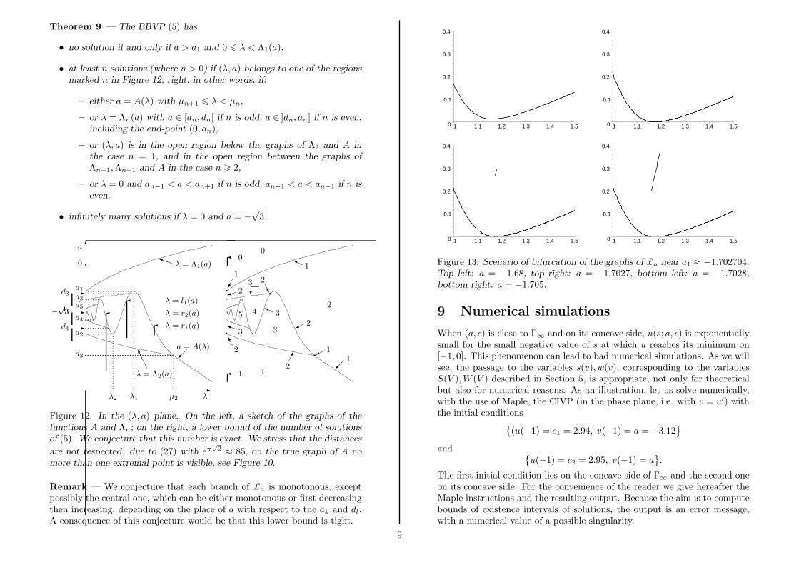
Figure 13: Scenario of bifurcation of the graphs of £a near a1 ≈ −1.702704.Top left: a = −1.68, top right: a = −1.7027, bottom left: a = −1.7028,bottom right: a = −1.705.

9 Numerical simulations

When (a, c) is close to Γ∞ and on its concave side, u(s; a, c) is exponentiallysmall for the small negative value of s at which u reaches its minimum on[−1, 0]. This phenomenon can lead to bad numerical simulations. As we willsee, the passage to the variables s(v), w(v), corresponding to the variablesS(V ),W (V ) described in Section 5, is appropriate, not only for theoreticalbut also for numerical reasons. As an illustration, let us solve numerically,with the use of Maple, the CIVP (in the phase plane, i.e. with v = u′) withthe initial conditions

{

(u(−1) = c1 = 2.94, v(−1) = a = −3.12}

and{

u(−1) = c2 = 2.95, v(−1) = a}

.

The first initial condition lies on the concave side of Γ∞ and the second oneon its concave side. For the convenience of the reader we give hereafter theMaple instructions and the resulting output. Because the aim is to computebounds of existence intervals of solutions, the output is an error message,with a numerical value of a possible singularity.

9

0

2

4

6

8

10

0.5 1 1.5 2 2.5 3 3.5 4 0

0.2

0.4

0.6

0.8

1 1.1 1.2 1.3 1.4 1.5

0

0.005

0.01

0.015

0.02

1.152 1.154 1.156 1.158 1.16 0

2e–05

4e–05

6e–05

8e–05

0.0001

0.00012

1.15466 1.1547 1.15472 1.15474 1.15476

Figure 14: Numerical graph of £a for a = −√

3, with successive enlarge-ments.

> restart:

> a:=-3.12: c1:=2.94: c2:=2.95:

> EqCroccoUV:=diff(u(s),s)=v(s),diff(v(s),s)=-s/u(s):

du

ds= v,

dv

ds= − s

u(29)

> SolCroccoUV:=proc(c)

> Sol:=dsolve({EqCroccoUV,u(-1)=c,v(-1)=a},{u(s),v(s)},

> numeric,output=listprocedure):

> SolU:=eval(u(s),Sol):

> SolU(50):

> end proc:

> SolCroccoUV(c1);

Error, (in SolU) cannot evaluate the solution further right of

-0.21850903e-2, probably a singularity

> SolCroccoUV(c2);

Error, (in SolU) cannot evaluate the solution further right of

0.99652635e-3, probably a singularity

The result for c1 is not correct since the solution must be defined for alls 6 0. The second result c2 is correct and predicts that £(a, c2) ≈ 0.001. Itis a fact, not completely elucidated, that the use of the logarithmic changeof variable w = lnu does not yield better numerical results: in the variables(w, v) the numerical solutions are still incorrect for c1 (and correct for c2).

> EqCroccoVW:=diff(w(s),s)=v(s)*exp(-w(s)),

> diff(v(s),s)=-s*exp(-w(s));

dw

ds= ve−w,

dv

ds= −se−w (30)

> SolCroccoVW:=proc(c)

> Sol:=dsolve({EqCroccoVW,w(-1)=ln(c),v(-1)=a},{w(s),v(s)},

> numeric,output=listprocedure):

> SolW:=eval(w(s),Sol):

> SolW(50):

> end proc:

> SolCroccoVW(c1);

Error, (in SolW) cannot evaluate the solution further right of

-0.21862961e-2, probably a singularity

> SolCroccoVW(c2);

Error, (in SolW) cannot evaluate the solution further right of

0.99531941e-3, probably a singularity

Following Section 5, we now consider the change of variable w = lnu anduse the variable v as an independent variable. This gives correct numericalresults.

> EqCroccoSW:=diff(s(v),v)=-exp(w(v))/s(v),diff(w(v),v)=-v/s(v);

ds

dv= −ew

s,

dw

dv= −v

s(31)

> SolCroccoSW:=proc(c)

> Sol:=dsolve({EqCroccoSW,w(a)=ln(c),s(a)=-1},{w(v),s(v)},

> numeric,output=listprocedure):

> SolS:=eval(s(v),Sol):

> SolS(10):

> end proc:

> SolCroccoSW(c1);

Error, (in SolS) cannot evaluate the solution further right of

2.7651840, probably a singularity

> SolCroccoSW(c2);

Error, (in SolS) cannot evaluate the solution further right of

-2.7726621, probably a singularity

10

We see that for c1, the solution w(v) is computed until the value v =2.7651840. Hence the numerical solution succeeded to pass exponentiallyclose to the axis u = 0 and to reflect on this axis and get a positive deriva-tive. The singularity encountered now at v = 2.7651840 is caused by the factthat system (31) is defined only in the half space s < 0. For s > 0 we mustreturn to the original variables u(s) and v(s). Hence we use the followingprocedure to evaluate £(a, c).

> Lambda:= proc(a,c)

> erreur:=0.0000000001:

> fSW:=dsolve({EqCroccoSW,w(a)=ln(c),s(a)=-1},{s(v),w(v)},

> numeric,stop_cond=[s(v)+erreur]):

> fSW(10);

> IC:=subs(%,[v,s(v),w(v)]):

> v0:=IC[1]: s0:=IC[2]: w0:=IC[3]:

> f:=dsolve({EqCroccoUV,u(s0)=exp(w0),v(s0)=v0},{u(s),v(s)},

> numeric,stop_cond=[u(s)-erreur]):

> f(50):

> subs(%,s):

> end proc:

This procedure is easy to understand. First system (31) is solved with ini-tial conditions w(a) = ln(c), s(a) = −1 as far as s 6 −erreur. Next, onecomputes the values v0, s0 = s(v0) and w0 = w(v0) such that the stop-ping condition s0 = −erreur is reached. Then system (29) is solved withinitial conditions u(s0) = ew0 , v(s0) = v0, as far as u > erreur. The proce-dure gives the value s1 such that the stopping condition u(s1) = erreur isattained. This value is a very good approximation of £(a, c).

> Lambda(a,c1);

Warning, cannot evaluate the solution further right of

2.7651840, stop condition #1 violated

Warning, cannot evaluate the solution further right of

10.012058, stop condition #1 violated

10.0120586420604791

> Lambda(a,c2);

Warning, cannot evaluate the solution further right of

-2.7726621, stop condition #1 violated

Warning, cannot evaluate the solution further right of

.99606109e-3, stop condition #1 violated

0.000996061092810659674

Hence, £(a, c1) ≈ 10.012 and £(a, c2) ≈ 0.001. The following instructionswhich use the procedure Lambda produce the numerical graph of £a fora = −

√3 and 1.15466 6 c 6 1.15476, see Figure 14 bottom right.

> a:=-sqrt(3): c1:=1.15466: c2:=1.15476: N:=200;

> for n from 0 to N do LLambda[n]:=c1+n*(c2-c1)/N,

> Lambda(a,c1+n*(c2-c1)/N) end do:

> L1:=[[LLambda[i]]$i=0..112]: L2:=[[LLambda[i]]$i=113..N]:

> plot([L1,L2],c1..c2,-.0000031..0.00012,thickness =4,

> color=black);

References

[1] Z. Belhachmi, B. Brighi and K. Taous, On the concave solutionsof the Blasius equation, Acta Math. Univ. Comenianae 69:2 (2000)199-214.

[2] E. Benoıt Ed., Dynamic Bifurcations, Proceedings Luminy 1990, Lect.Notes Math. 1493 Springer-Verlag, 1991.

[3] H. Blasius, Thesis, Gottingen (1907).

[4] H. Blasius, Grenzschichten in Flussigkeiten mit kleiner Reibung,Zeitschr. Math. Phys. 56 (1908) 1-37.

[5] B. Brighi, Deux problemes aux limites pour l’equation de Blasius,Revue Math. Ens. Sup. 8 (2001) 833-842.

[6] B. Brighi, A. Fruchard and T. Sari, On the Blasius Problem, Adv.

Differential Equations 13 (2008), no. 5-6, 509–600.

[7] L. Crocco, Sull strato limite laminare nei gas lungo una lamina plana,Rend. Math. Appl. Ser. 5 21 (1941) 138-152.

[8] P. Hartman, Ordinary Differential Equations, Wiley, 1964.

[9] M. Y. Hussaini and W. D. Laikin, Existence and non-uniqueness ofsimilarity solutions of a boundary layer problem, Quart. J. Mech. Appl.

Math. 39:1 (1986) 15-24.

[10] M. Y. Hussaini, W. D. Laikin and A. Nachman, On similaritysolutions of a boundary layer problem with an upstream moving wall,SIAM J. Appl. Math. 47:4 (1987) 699-709.

[11] C. Lobry, T. Sari and S. Touhami, On Tykhonov’s theorem for con-vergence of solutions of slow and fast systems, Electron. J. Differential

Equations 19 (1998) 1-22.

[12] O. A. Oleinik, V. N. Samokhin, Mathematical Models in Boundary

Layer Theory, Applied Mathematics and Mathematical Computations15, Chapman& Hall/CRC, Washington (1999)

11

[13] E. Soewono, K. Vajravelu and R.N. Mohapatra, Existence andnonuniqueness of solutions of a singular non linear boundary layer prob-lem, J. Math. Anal. Appl. 159 (1991) 251-270.

[14] A. N. Tikhonov, Systems of differential equations containing smallparameters multiplying the derivatives, Mat. Sb. 31 (1952) 575-586.

[15] W. Wasow, Asymptotic Expansions for Ordinary Differential Equa-

tions, Krieger, New York (1976).

[16] H. Weyl, On the differential equations of the simplest boundary-layerproblems, Ann. Math. 43 (1942) 381-407.

Address of the authors:Laboratoire de Mathematiques, Informatique et Applications, EA3993Faculte des Sciences et Techniques, Universite de Haute Alsace4, rue des Freres Lumiere, F-68093 Mulhouse cedex, France

Current address for T. Sari:EPI MERE INRIA/INRA, UMR MISTEASupAgro Bat 21, 2 Place Pierre VialaF-34060 Montpellier cedex, France

E-addresses:Bernard.Brighi@uha.fr, Augustin.Fruchard@uha.fr, Tewfik.Sari@uha.fr

12