The Blanchet-Khovanov algebras - uni-bonn.de
40
THE BLANCHET-KHOVANOV ALGEBRAS MICHAEL EHRIG, CATHARINA STROPPEL, AND DANIEL TUBBENHAUER Dedicated to Christian Blanchet’s sixtieth birthday Abstract. Blanchet introduced certain singular cobordisms to fix the func- toriality of Khovanov homology. In this paper we introduce graded algebras consisting of such singular cobordisms ` a la Blanchet. As the main result we give algebraic versions of these algebras using the combinatorics of arc diagrams. Contents 1. Introduction 1 2. sl 2 -foams and sl 2 -web algebras 4 2.1. Webs, foams and TQFT’s 4 2.2. Blanchet’s singular TQFT construction 8 2.3. An action of the quantum group ˙ U q (gl ∞ ) 12 2.4. sl 2 -web algebras 13 2.5. Web bimodules 16 3. Blanchet-Khovanov algebras 17 3.1. Combinatorics of arc diagrams 17 3.2. The Blanchet-Khovanov algebras as graded K-vector spaces 19 3.3. Multiplication of the Blanchet-Khovanov algebra 20 3.4. Bimodules for Blanchet-Khovanov algebras 23 4. Equivalences 26 4.1. Some useful lemmas 26 4.2. The action of the quantum group ˙ U q (gl ∞ ) and arc diagrams 30 4.3. The cup basis 30 4.4. Proof of the main result 32 4.5. The proof of the graded isomorphism 33 References 38 1. Introduction For an arbitrary field K we consider the sl 2 -web algebra W (web algebra for short). This is a graded K-algebra which naturally appears as an algebra of singular cobordisms. In particular, it is of topological origin. The underlying category of singular cobordisms was used in [2] by Blanchet to fix the functoriality of Khovanov homology. Its objects are certain trivalent graphs and its morphisms are singular cobordisms whose boundary are such trivalent graphs. We call these singular cobordisms sl 2 -foams (or foams for short). Note that Blanchet’s category is a sign modified version of the original cobordism category which describes Khovanov homology and which was for instance used by Bar-Natan in his formulation of Khovanov homology, see [1]. The fact that such a twist in the definition of Khovanov homology solves the functoriality leaves the question whether this could also be fixed algebraically using the original construction of Khovanov involving his arc algebra, see [15]. We therefore suggest here to study a certain signed (with highly non-trivial sign modifications) version H F of Khovanov’s original algebra, which we call the Blanchet-Khovanov algebra. This is a graded K-algebra defined diagrammatically 1 arXiv:1510.04884v1 [math.RT] 16 Oct 2015
Transcript of The Blanchet-Khovanov algebras - uni-bonn.de

THE BLANCHET-KHOVANOV ALGEBRAS
MICHAEL EHRIG, CATHARINA STROPPEL, AND DANIEL TUBBENHAUER
Dedicated to Christian Blanchet’s sixtieth birthday
Abstract. Blanchet introduced certain singular cobordisms to fix the func-
toriality of Khovanov homology. In this paper we introduce graded algebrasconsisting of such singular cobordisms a la Blanchet. As the main result we givealgebraic versions of these algebras using the combinatorics of arc diagrams.
Contents
1. Introduction 12. sl2-foams and sl2-web algebras 42.1. Webs, foams and TQFT’s 42.2. Blanchet’s singular TQFT construction 82.3. An action of the quantum group Uq(gl∞) 122.4. sl2-web algebras 132.5. Web bimodules 163. Blanchet-Khovanov algebras 173.1. Combinatorics of arc diagrams 173.2. The Blanchet-Khovanov algebras as graded K-vector spaces 193.3. Multiplication of the Blanchet-Khovanov algebra 203.4. Bimodules for Blanchet-Khovanov algebras 234. Equivalences 264.1. Some useful lemmas 264.2. The action of the quantum group Uq(gl∞) and arc diagrams 304.3. The cup basis 304.4. Proof of the main result 324.5. The proof of the graded isomorphism 33References 38
1. Introduction
For an arbitrary field K we consider the sl2-web algebra W (web algebra forshort). This is a graded K-algebra which naturally appears as an algebra of singularcobordisms. In particular, it is of topological origin. The underlying category ofsingular cobordisms was used in [2] by Blanchet to fix the functoriality of Khovanovhomology. Its objects are certain trivalent graphs and its morphisms are singularcobordisms whose boundary are such trivalent graphs. We call these singularcobordisms sl2-foams (or foams for short). Note that Blanchet’s category is asign modified version of the original cobordism category which describes Khovanovhomology and which was for instance used by Bar-Natan in his formulation ofKhovanov homology, see [1]. The fact that such a twist in the definition of Khovanovhomology solves the functoriality leaves the question whether this could also befixed algebraically using the original construction of Khovanov involving his arcalgebra, see [15].
We therefore suggest here to study a certain signed (with highly non-trivial
sign modifications) version HF of Khovanov’s original algebra, which we call theBlanchet-Khovanov algebra. This is a graded K-algebra defined diagrammatically
1
arX
iv:1
510.
0488
4v1
[m
ath.
RT
] 1
6 O
ct 2
015

2 MICHAEL EHRIG, CATHARINA STROPPEL, AND DANIEL TUBBENHAUER
via explicit multiplication rules on a distinguished set of basis vectors similar to thefamily of algebras from [4] or [12].
The main result of the paper is then that HF is an algebraic counterpart of W:
Theorem. There is an equivalence of graded, K-linear 2-categories
Φ : W-biModpgr
∼=−→ HF-biModpgr
induced by an isomorphism of graded algebras
Φ : W◦ → HF,
where W◦ is a certain subalgebra of W. �
This provides a direct link between the topological and the algebraic point ofview. As a consequence, computations (which are hard to do in practice on thetopological side) can be done on the algebraic side, whereas the associativity (anon-trivial fact on the algebraic side) is clear from the topological point of view.
The set-up in more details. In his pioneering work [15], Khovanov introduced theso-called arc algebra Hm. One of his main purposes was to extend his celebratedcategorification of the Jones polynomial [14] to tangles. To a given tangle with2m bottom boundary points and 2m′ top boundary points one associates a certaincomplex of graded Hm-Hm′ -bimodules. He showed that the chain homotopy equiva-lence class of this complex is an invariant of the tangle. Moreover, tensoring with acertain Hm-module from the left and a certain Hm′ -module from the right producesa complex which is still an invariant. Furthermore, on the level of Grothendieckgroups this invariant descends to the Kauffman bracket of the tangle.
In this set-up it makes sense to ask if cobordisms between tangles correspond tonatural transformations between bimodules. Or said in other words, whetherthere is a 2-functor from the 2-category of tangles to a certain 2-category ofH =
⊕m∈Z≥0
Hm-bimodules. This is often called functoriality.
In a series of papers [4], [5], [6], [7] and [8] Brundan and the second author studieda generalization HΛ of the arc algebra revealing that Khovanov’s arc algebra has,left aside its knot theoretical origin, interesting representation theoretical, algebraicgeometrical and combinatorial properties. These algebras HΛ were defined usingan algebraic approach via combinatorics of arc diagrams, i.e. certain diagramsconsisting of embedded lines in R2 inspired by the diagrams for Temperley-Liebalgebras.
This series of results has led to several variations and generalizations of Khovanov’soriginal formulation, utilized in a large body of work by several researchers (includingthe authors of this paper), e.g. an sl3-variation considered in [24], [31] and [32],and an sln-variation studied in [23], all of them having relations to (cyclotomic)KL-R algebras as in [17] or [28], and link homologies in the sense of Khovanov andRozansky [18]. There is also the gl1|1-variation developed in [29] with relations to
the Alexander polynomial as well as a type D-version introduced in [11] and [12]with connections to the representation theory of Brauer’s centralizer algebras andorthosymplectic Lie superalgebras.
A fact we like to stress about the sl3/sln-variations is that their graded 2-cate-gories of biprojective, finite-dimensional modules are equivalent to certain graded2-categories of sl3/sln-foams, the analogues of Bar-Natan’s cobordism category [1]studied e.g. in [16], [21], [25] and [26] from the viewpoint of link homologies. Such atopological description for the type D-version is still missing, which forced the firsttwo authors in [12] to show “by hand” that the type D algebras are associative.
We like to stress that Khovanov’s original construction as well as Bar-Natan’s re-formulation from [1] are not functorial, but are functorial up to signs, see [1], [13], [27]

THE BLANCHET-KHOVANOV ALGEBRAS 3
or [30]. It became clear that Bar-Natan cobordisms miss some subtle extra signs(see for example [10] for the first fix of functoriality using “disoriented” cobordisms).
A solution to this problem, that is of key interest for us, was provided by Blanchetin [2]. He formulated Khovanov’s link homology using certain singular cobordisms,that we call (sl2-)foams, which, by construction, include highly non-trivial signs fixingthe functoriality of Khovanov’s link homology. Moreover, Blanchet’s formulation fitsneatly into the framework of graded 2-representations of the categorified quantumgroup in the sense of [17], as it was shown in [21].
Using Blanchet’s construction it makes sense to define “foamy” versions ofKhovanov’s arc algebra, which we denote by W~k and which we call (sl2-)webalgebras. We set W =
⊕~k∈bl� W~k. The web algebras W~k and W are graded
K-algebras defined using Blanchet’s singular cobordisms and the multiplication isgiven by composition of singular cobordisms (for our conventions see Section 2).The signs within this multiplication are quite sophisticated, e.g. even merges (whichare quite easy in the formulations of [4] and [12]) can come with a sign.
Unfortunately calculating in W~k and W is very hard. Indeed, it is not even clearwhat a basis of W~k or W is - left aside the question how to rewrite an arbitraryfoam in terms of some basis. Thus, the main purpose of this paper is to give algebraiccounterparts of W~k and W, denoted by HF
Λ and HF =⊕
Λ∈bl� HFΛ where these
questions about bases are easy. We call the algebraic counterparts, which are buildup using certain combinatorics of arc diagrams, Blanchet-Khovanov algebras.
The proof of our main theorem relies on the rather subtle Theorem 4.18 whichneeds careful treatment of all involved signs. The whole Subsection 4.5 is devotedto its proof. Our main theorem clarifies algebraically the deficiency in the originaltheory. For brevity, we stop our investigation here although several natural questionsremain open, e.g. the representation theoretical meaning of the Blanchet-Khovanovalgebras (for instance, its connection to category O). See also Remark 4.20.
Moreover, we tried to give a reasonably self-contained exposition.
Conventions used throughout.
Convention 1.1. Let K denote a field of arbitrary characteristic. By an algebrawe always mean a non-necessary finite-dimensional, non-necessary unital K-algebraA. We also do not assume that such A’s are associative and it will be a non-trivialfact that all A’s which we consider are actually associative. Given two algebras Aand B, then an A-B-bimodule is a K-vector space M with a left action of A anda right action of B in the usual compatible sense. If A = B, then we also writeA-bimodule for short. We call an A-B-bimodule M biprojective, if it is projective asa left A-module as well as a right B-module (such finitely generated bimodules arecalled sweet in [15, Subsection 2.6]). We denote the category of finite-dimensionalA-bimodules by A-biMod. Diagrammatic left actions will be given by acting onthe bottom and diagrammatic right actions by acting on the top. NConvention 1.2. By a graded algebra we mean an algebra A which decomposesinto graded pieces A =
⊕i∈ZAi such that AiAj ⊂ Ai+j for all i, j ∈ Z. Given two
graded algebras A and B, we study (and only consider) graded A-B-bimodules, i.e.A-B-bimodules M =
⊕i∈ZMi such that AiMjBk ⊂Mi+j+k for all i, j, k ∈ Z. We
also set Mi{s} = Mi−s for s ∈ Z (thus, positive integers shift up).If A is a graded algebra and M is a graded A-bimodule, then M obtained from
M by forgetting the grading is in A-biMod. Given such A-bimodules M,N , then
(1) HomA-biMod(M,N) =⊕s∈Z
Hom0(M,N{s}).
Here Hom0 means all degree-preserving A-homomorphisms, i.e. f(Mi) ⊂ Ni. N
4 MICHAEL EHRIG, CATHARINA STROPPEL, AND DANIEL TUBBENHAUER
Convention 1.3. We consider three diagrammatic calculi in this paper: sl2-webs(webs for short) in the sense of [9] and [20], foams whose definition is motivatedfrom [2] and [16], and arc diagrams in the sense of [4] and [6]. Our reading conventionfor all of these is from bottom to top and right to left. Moreover, we sometimesillustrate local pieces. The corresponding diagram is meant to be the identity orarbitrary outside of the displayed part (which one will be clear from the context). N
Remark 1.4. We use colors in this paper. It is only necessary to distinguish colorsfor webs and foams. For the readers with a black-and-white version: we illustratecolored web edges using dashed lines, while colored foam facets appear shaded. N
Acknowledgements: We like to thank David Rose and Nathalie Wahl for helpfulconversations. M.E. and D.T. thank the whiteboard in their office for many helpfulillustrations.
2. sl2-foams and sl2-web algebras
In this section we introduce the foam 2-category F and the web algebra W inthe spirit of Khovanov [15], but using foams a la Blanchet [2].
2.1. Webs, foams and TQFT’s. We start by recalling the definition of a web.
For this purpose, we denote by bl the set of all vectors ~k = (ki)i∈Z ∈ {0, 1, 2}Zwith ki = 0 for |i| � 0. Abusing notation, we also sometimes write ~k = (ka, . . . , kb)
for some fixed part of ~k (with a < b ∈ Z) where it is to be understood that allnon-displayed entries are zero. By convention, the empty vector ∅ ∈ bl is the unique
vector containing only zeros. We consider ~k ∈ bl as a set of discrete labeled pointsin R× {0} (or in R× {±1}) by putting the symbols ki at position (i, 0) (or (i,±1)).
Definition 2.1. A web is an embedded labeled, oriented, trivalent graph which canbe obtained by gluing (whenever this makes sense and the labels fit) or juxtapositionof finitely many of the following pieces.
1
1
,
2
2
,
2
1 1
,
2
1 1
In particular, we do not allow downwards pointing edges. We assume that websare embedded in R× [−1, 1] such that each edge starts/ends either in a trivalentvertex or at the boundary of the strip at the points (i,±1). We assume that thepoints at (i,±1) are labeled 1 or 2. In particular, these webs have distinguished
bottom ~k and top ~l boundary which we will throughout denote from left to right
by ~k = (ka, . . . , kb) and ~l = (la′ , . . . , lb′) where ki is the label at (i,−1) and li is thelabel at (i, 1).
Edges come in two different version, i.e. ordinary edges which are only allowedto touch boundary points labeled 1, and phantom edges which are only allowed totouch boundary points labeled 2. We draw phantom edges dashed (and colored);one should think of them as “non-existing”.
We denote the K-vector space with basis consisting of all webs with bottom
boundary ~k and top boundary ~l by HomF(~k,~l). Given ~k ∈ bl, we denote by
1~k ∈ HomF(~k,~k) the identity web on ~k. Note that we call only the basis vectors in
HomF(~k,~l) webs (and not their K-linear combinations). Furthermore, we call a webthat only contains phantom edges empty. N
By a surface we mean a marked, orientable, compact surface with possiblefinitely many boundary components and with finitely many connected components.

THE BLANCHET-KHOVANOV ALGEBRAS 5
Additionally, by a trivalent surface we understand the same as in [16, Subsection 3.1],i.e. certain embedded, marked, singular cobordisms whose boundaries are webs.
Precisely, fix the following data denoted by S:
(I) A surface S with connected components divided into two sets S1, . . . , Srand Sp
1 , . . . , Spr′ . The former are called ordinary surfaces and the latter are
called phantom surfaces.(II) The boundary components of S are partitioned into triples (Ci, Cj , C
pk )
such that each triple contains precisely one boundary component Cpk of a
phantom surface.(III) The three circles Ci, Cj and Cp
k in each triple are identified via diffeomor-phisms ϕij : Ci → Cj and ϕjk : Cj → Cp
k .(IV) A finite (possible empty) set of markers per connected components S1, . . . , Sr
and Sp1 , . . . , S
pr′ that move freely around its connected component.
Definition 2.2. Let S be as above. The closed singular trivalent surface fc = fScattached to S is the CW-complex obtained as the quotient of S by the identificationsϕij and ϕjk. We call all such fc’s closed pre-foams (following [16]) and their markersdots. A triple (Ci, Cj , C
pk ) becomes one circle in fc which we call a singular seam,
while the interior of the connected components S1, . . . , Sr and Sp1 , . . . , S
pr′ are facets
of fc, called ordinary facets respectively phantom facets. We embed these pre-foamsinto R2 × [−1, 1] in such a way that the three annuli glued to a singular seam areconsistently oriented (which induces an orientation on the singular seam, compareto (2)). We consider closed pre-foams modulo isotopies in R2 × [−1, 1]. N
Example 2.3. Consider two spheres with two punctures respectively one puncture.The sphere with one puncture is assumed to be a phantom sphere (we color phantomfacets in what follows).
S1
C1 C2
Sp1
Cp3
glue//
f
Then the pre-foam on the right is obtained by identifying the three boundary circles.Another example of a closed pre-foam is given below in the proof of Lemma 2.12(where we leave it to the reader to identify the precise labels). N
The pre-foams we have constructed so far are all closed. We will need non-closedpre-foams as well. To this end, we follow [16, Subsection 3.3] and consider a planeP ∼= R2 ⊂ R3. We say that P intersects a closed pre-foam fc generically, if P ∩ fcis a web (forgetting the orientations). We assume that P × [−1, 1] is embedded intoR2 × [−1, 1] in the evident way.
Definition 2.4. A non-closed pre-foam f is the intersection of P × [−1, 1] withsome closed foam fc such that P × {±1} intersects fc generically. We consider suchpre-foams modulo isotopies in R2× [−1, 1] which fix the horizontal boundary. We seesuch non-closed pre-foam f as a singular cobordism between (P×{−1})∩fc (bottom,source) and (P ×{+1})∩ fc (top, target) embedded in R2× [−1, 1]. Moreover, thereis an evident composition g ◦f via gluing and rescaling (if the top boundary of f andthe bottom boundary of g coincide). Similarly, we construct pre-foams embedded inR× [−1, 1]× [−1, 1] with vertical boundary components. These vertical boundarycomponents should be the boundary of the webs at the bottom/top times [−1, 1]

6 MICHAEL EHRIG, CATHARINA STROPPEL, AND DANIEL TUBBENHAUER
and we now take everything modulo isotopies that preserve the vertical boundaryas well as the horizontal boundary. N
We call pre-foam parts ordinary, if they do not contain singular seams or phantomfacets, and we call pre-foam parts ghostly, if they only contain phantom facets.
Example 2.5. Pre-foams can be seen as singular surfaces (with oriented, singularseams) in R× [−1, 1]× [−1, 1] such that the bottom boundary and the top boundaryare webs with facets colored as follows:
:
1
1
→1
1
and :
2
2
→2
2
The leftmost facet is an ordinary facet. Whereas the rightmost facet is a phantomfacet and the reader might think of it as “non-existing” (similar to a phantomedge) - they only encode signs. Moreover, the only vertical boundary components ofpre-foams f come from the boundary points of webs times [−1, 1]. All generic slicesof pre-foams are webs, and the singularities of f are all locally of the following form(where the other orientations of the facets/seams are also allowed)
(2) :
2
1 1
→2
1 1
and � :
2
1 1
→2
1 1
Here we have only indicated the orientation of the phantom facet, since the othertwo orientations are fixed by this choice due to our construction. Note that it sufficesto indicate the orientation of the singular seams in what follows. Such pre-foamscan carry dots that freely move around its facets:
•=
•and
•=
•N
Remark 2.6. Pre-foams are considered modulo boundary preserving isotopies thatdo preserve the condition that each generic slice is a web. These isotopies form afinite list: isotopies coming from the two cobordism theories associated to the twodifferent types of facets (see for example [19, Section 1.4]) and isotopies comingfrom isotopies of the singular seams seen as tangles in R2 × [−1, 1]. N
To work with the 2-category of foams it will be enough (for our purposes) toconsider its image under a certain TQFT functor defined by Blanchet [2]. Recallthat equivalence classes of TQFT’s for surfaces are in one-to-one correspondencewith isomorphism classes of (finite-dimensional, associative) commutative Frobeniusalgebras (the reader unfamiliar with this correspondence might consult Kock’sbook [19], which is our main source for these kind of TQFT’s in this paper). Given aFrobenius algebra A corresponding to a TQFT, i.e. a functor TA from the categoryof surfaces to the category of K-vector spaces, then the association is as follows.To a disjoint union of m circles one associates the m-fold tensor product A⊗m. To

THE BLANCHET-KHOVANOV ALGEBRAS 7
a cobordism Σ with distinguished incoming and outgoing boundary componentsconsisting of, let us say, m and m′ circles, we assign a K-linear map from A⊗m toA⊗m′ . Hereby the usual cup/cap respectively pants cobordisms correspond to theunit, counit, multiplication and comultiplication maps, see [19]. These are the basicpieces of every cobordism. Then the TQFT assigns to Σ a K-linear map
TA(Σ): A⊗m → A⊗m′ ,which is obtained by decomposing Σ into basic pieces.
The commutative Frobenius algebras we need are
(3) A1 = K[X]/(X2), A2 = K
with induced multiplications, counits εi(·) and comultiplications ∆i(·) given via
ε1(1) = 0, ε1(X) = 1, ε2(1) = −1,
∆1(1) = 1⊗X +X ⊗ 1, ∆1(X) = X ⊗X, ∆2(1) = −1⊗ 1.
Thus, we have the traces
tr1(1⊗ 1) = tr1(X ⊗X) = 0, tr1(1⊗X) = tr1(X ⊗ 1) = 1, tr2(1⊗ 1) = −1.(4)
We associate the Frobenius algebra A1 to the ordinary parts and the Frobeniusalgebra A2 to the phantom parts of a pre-foam f .
Example 2.7. In our context, dots correspond to multiplication by X or 0:
•TA17−→ ·X : A1 → A1, •
TA27−→ ·0: A2 → A2.
Moreover, if we view a K-linear map φ : K→ A⊗mi as φ(1) ∈ A⊗mi , then
TA17−→ 1 ∈ A1, •TA17−→ X ∈ A1,
TA27−→ 1 ∈ A2.(5)
Here we have from left to right ι1, (·X) ◦ ι1 and ι2 as maps. These are sometimescalled units. The counits εi are obtained by flipping the pictures. N
Note that the values of the non-closed surfaces can be determined by closingthem in all possible ways using (5) and its dual. Here and throughout, we say forshort that a relation a = b lies in the kernel of a TQFT functor F , if F(a) = F(b)as K-linear maps.
Lemma 2.8. The ordinary and ghostly sphere relations and the cyclotomic relationsas displayed here
= 0,
•= 1, = −1,(6)
• • = 0, • = 0.(7)

8 MICHAEL EHRIG, CATHARINA STROPPEL, AND DANIEL TUBBENHAUER
as well as the ordinary and ghostly neck cutting relations
=
•+
•and = −(8)
are in the kernel of TA1(ordinary) respectively of TA2
(ghostly). Consequently,the TQFT TA1
kills cobordisms with 2 or more dots, while the TQFT TA2kills
cobordisms with 1 or more dots. �Proof. Via direct calculation. For instance, the ordinary respectively ghostly neckcutting relations decompose the identity map as id = (·X) ◦ ι1 ◦ ε1 + ι1 ◦ ε1 ◦ (·X)respectively id = −ι2 ◦ ε2 with units ιi and counits εi as in (5). �
The neck cutting relations (8) give a topological interpretation of dots as ashorthand notation for handles, see also [1, (4)].
2.2. Blanchet’s singular TQFT construction. The following definition followsthe construction given by Blanchet, see [2, Subsection 1.5].
We want to construct a TQFT functor T on the category whose objects are websas in Definition 2.1. To this end, let pF denote the 1-category whose objects arewebs and whose 1-morphisms are pre-foams (composition is gluing of pre-foams).Moreover, we define for a, b, c, d ∈ K
αA1: A1 ⊗A1 → A1, (a+bX)⊗ (c+ dX) 7→ (a+ bX)(c− dX),
αA2: A2 → A1, 1 7→ 1.
(9)
Definition 2.9. Let TA1and TA2
denote the TQFT’s associated to A1 and A2
from (3). Given a closed pre-foam fc, let fc = f1∪f2 be the pre-foam obtained bycutting fc along the singular seams (of which we assume to have m in total). Heref1 is the surface which in fc is attached to the ordinary parts and f2 is the surfacewhich in fc is attached to phantom parts. Note that the boundary of f1 splits intoσ+i and σ−i for each i ∈ {1, . . . ,m}. Which one is which depends on the orientation
of the singular seam: use the right hand rule with the fore finger pointing in thedirection of the singular seam and the middle finger pointing in direction of theattached phantom facet, then the thump points in direction of σ+
i . In contrast, f2
has only boundary components σi for each i ∈ {1, . . . ,m}. Now
TA1(f1) ∈
m⊗i=1
(TA1(σ+i )⊗ TA1
(σ−i )) ∼= (A1 ⊗A1)⊗m,
TA2(f2) ∈
m⊗i=1
TA2(σi) ∼= A⊗m2 .
Let tr1 : A1 → Z be as in (4), and let αA1, αA2
be as in (9). Then we set
T(fc) = (tr1)⊗m(α⊗mA1(TA1(f1))⊗ α⊗mA2
(TA2(f2))) ∈ K⊗m ∼= K.This gives a well-defined functor on closed pre-foams assigning to each such fc avalue T(fc) ∈ K. N
A crucial insight of Blanchet is that this extends to non-closed pre-foams:
Theorem 2.10. The construction from Definition 2.9 can be extended to a TQFTfunctor T : pF → K-Vect. �Proof. This follows by the universal construction from [3]. �

THE BLANCHET-KHOVANOV ALGEBRAS 9
Note the following properties of pre-foams f , which follow by construction.
(I) The topological reduction f obtained by removing all phantom facets of f isthe cobordism theory corresponding to A1 from (3).
(II) The phantom f obtained by removing all 1-labeled facets of f is the cobor-dism theory corresponding to A2 from (3).
Hence, the relations from (6), (7) and (8) are also in the kernel of the functor T .The following lemmas give some additional relations in the kernel of T .
Lemma 2.11. Let f be the pre-foam obtained from a pre-foam f by reversing theorientation of a singular seam. Then f + f = 0 is in the kernel of T . �Proof. This follows because switching the orientation of a singular seam swaps theattached parts of σ+
1 and σ−1 . This changes the sign because this swaps the twocopies of A1 in the source of αA1
from (9) (we note that the case b = d = 0 is killedby applying the trace ε1 in the formula for T(fc)). �Lemma 2.12. The sphere relations, i.e.
•
•
a
b
=
1, if a = 1, b = 0,
−1, if a = 0, b = 1,
0, otherwise,
(10)
are in the kernel of T . �Proof. We prove the case a = 0, b = 1. The others are similar and omitted forbrevity. Decompose the sphere fc into (t=thump, f=fore finger, m=middle finger)
•
t
f
m//
•
f1f2
σ1
σ+1
σ−1
Now, because of the assignment in (5), we have TA1(f1) = 1⊗X and TA2(f2) = 1.Thus, αA1(TA1(f1)) = −X and αA2(TA2(f2)) = 1, both considered in A1. Applyingthe trace tr1 to −X ⊗ 1 gives −1 as in (10). �Lemma 2.13. The bubble removals (a “sphere” in a phantom plane; the top dotsare meant to be on the front facets and the bottom dots on the back facets)
•= = −
•(11)
= 0 =•
•(12)

10 MICHAEL EHRIG, CATHARINA STROPPEL, AND DANIEL TUBBENHAUER
are in the kernel of T . The neck cutting relation
=
•
−
•
(13)
(with top dot on the front facet and bottom dot on the back facet) is also in thekernel of T . Furthermore, the squeezing relation
= −(14)
and the dot migrations
• = − •and • = − •
(15)
as well as the ordinary-to-phantom neck cutting relations (in the leftmost picture theupper closed circle is an ordinary facet, while the lower closed circle is a phantomfacet, and vice versa for the rightmost picture)
= − and = −(16)
are also in the kernel of T . �
The leftmost situation in (13) is called a cylinder - as all local parts of pre-foams
f such that the corresponding part in f is a cylinder. Note that the squeezingrelation (14) enables us to use the neck cutting (13) on more general cylinders (withpossible internal phantom facets).

THE BLANCHET-KHOVANOV ALGEBRAS 11
Proof. We only prove the left equation in (16). First note that we have to considerall possible ways to close the non-closed pre-foam on the left-hand and on theright-hand side of the equation. We consider the closing
•
and −
•
since all other possibilities give zero (as the reader might want to check). By (6),the right-hand closed pre-foams evaluate to −(1 · (−1)). Now, we can use (8):
•
=
•
•+
•
•
(10)=
•
•
The bottom sphere evaluates to −1 because of (10). Moreover, performing the samesteps as in the proof of Lemma 2.12, we see that the top sphere also evaluates to−1. Thus, the left-hand and the right-hand side evaluate to the same value. Thisshows that the first equation in (16) is in the kernel of T . The other relations areverified similarly, see also [2, Lemma 1.3] or [21, Subsection 3.1]. �
If we define a grading on the TQFT-modules by setting deg(1) = −1 anddeg(X) = 1, then the TQFT TA1 respects the grading, where the degree of acobordism Σ is given by deg(Σ) = −χ(Σ) + 2 · dots. Here χ(Σ) is the topologicalEuler characteristic of Σ, that is, the number of vertices minus the number ofedges plus the number of faces of Σ seen as a CW complex, and “dots” is the totalnumber of dots. Additionally, we can see the TQFT TA2
as being trivially graded.Motivated by this we define the following.
Definition 2.14. Given a pre-foam f , we define its degree
deg(f) = −χ(f) + 2 · dots + 12vbound,
where vbound is the total number of vertical boundary components. If f is the
empty cobordism, then, by convention, χ(f) = 0. N

12 MICHAEL EHRIG, CATHARINA STROPPEL, AND DANIEL TUBBENHAUER
Example 2.15. For example,
deg
•
= 2, deg
= 1.
The leftmost pre-foam is called a dotted cup (the name will become clear inLemma 2.26), while the rightmost pre-foam is called a saddle (there are alsosaddles obtained by flipping the picture upside down). Furthermore, we have
deg
= −1 = deg
for the pre-foams called cup respectively cap. N
The 2-category we like to study is the following one, which we cook up from T .
Definition 2.16. Let F be the K-linear 2-category given by:
• The objects are all ~k ∈ bl together with a zero object.
• The 1-morphisms spaces HomF(~k,~l) is the K-vector space on basis consisting
of all webs whose bottom boundary is ~k and whose top boundary is ~l (we
have HomF(~k,~l) = 0 iff ka + · · ·+ kb 6= la′ + · · ·+ lb′).• The 2-morphisms spaces 2HomF(u, v) for u, v ∈Web is the K-linear span
of all pre-foams with bottom boundary u and top boundary v.• Composition of webs v ◦ u is given by stacking v on top of u, vertical
compositions g ◦ f of pre-foams by stacking g on top of f , horizontalcomposition g⊗ f by putting g to the right of f (whenever those operationsmake sense).• We take everything modulo the relations in the kernel of TA1 and TA2
from (6), (7) and (8), as well as the relations found in Lemmas 2.11, 2.12and 2.13.
Since the relations are degree preserving, F is a graded, K-linear 2-category bytaking the degree from Definition 2.14. N
We call the 2-morphisms in F foams. Moreover, all notions we had for pre-foamscan be adapted to the setting of foams and we do so in the following. Note that theobjects and the 1-morphisms of F form a K-linear 1-category W.
2.3. An action of the quantum group Uq(gl∞). We denote by Uq(gl∞) the
1-category whose objects are given by ~k ∈ bl and whose 1-morphisms are generated
by pairwise orthogonal idempotents 1~k, and by E(r)i 1~k and F
(r)i 1~k for ~k ∈ bl, i ∈ Z
and r ∈ Z>0 (the generators E(r)i 1~k and F
(r)i 1~k are called the divided powers)
modulo some relations which are analogs of the relations in the quantum groupUq(gl∞) (see [22, Chapter 23]). We note that there exists a unique 1~l such that
1~lE(r)i 1~k 6= 0 and 1~lF
(r)i 1~k 6= 0. This enable us to write 1~k only on one side of any
expression. Now, there is a K-linear functor
ΦWHowe : Uq(gl∞)→W

THE BLANCHET-KHOVANOV ALGEBRAS 13
given on objects by ΦWHowe(
~k) = ~k, and on 1-morphisms by ΦWHowe(1~k) = 1~k and
(where we use a simplified, “rectangular”, notation for webs):
Ei1~kΦW
Howe7−→2 1
1 2
i
,
1 0
0 1
i
,
1 1
0 2
i
,
2 0
1 1
i
, E(2)i 1~k
ΦWHowe7−→
2 0
0 2
i
Fi1~kΦW
Howe7−→21
12
i
,
0 1
1 0
i
,
1 1
2 0
i
,
0 2
1 1
i
, F(2)i 1~k
ΦWHowe7−→
0 2
2 0
i
(17)
Here the generators Ei1~k, Fi1~k, E(2)i 1~k and F
(2)i 1~k are sent to the local (between
strand i and i + 1) pictures above (we have displayed all possibilities depending
on ~k at position ki and ki+1). Moreover, all higher divided powers E(r)i 1~k, F
(r)i 1~k
for r > 2 are sent to zero. We call webs that arise as ΦWHowe(X), for X being any
composition of the 1~k, E(r)i 1~k, F
(r)i 1~k generators, EF -generated, and, on the other
hand, webs F -generated, if X is any composition of only 1~k, F(r)i 1~k generators. For
details about the functor ΦWHowe we refer to [9, Section 5].
Example 2.17. If ~k = (0, 0, 1, 0, 2, 0, 1, 2, 0, 0), then E1E0E−1E2F01~k is sent to
0 0 1 0 2
00 1 2 0 0
0 0 1 1 1 1 1 1 0 0
Here the first entry 2 is assumed to be at position 0. N2.4. sl2-web algebras. Now we define the following “algebraic” version of F. Tothis end, let ` ∈ Z≥0 and let ω` = (1, . . . , 1, 0, . . . , 0) with ` numbers equal 1. Fix~k and let Cup(~k) = HomF(2ω`,~k) and Cap(~k) = HomF(~k, 2ω`). Basis elements ofthese are called cup webs respectively cap webs. For diagrams in the multiplicationprocess of W described below, we also need cup-ray webs as well, i.e. elements of
CupRay(~k) = HomF(ω`+`′ + ω`,~k) for ~k ∈ bl (and similarly defined cap-ray webs).
Definition 2.18. Let u, v ∈ Cup(~k),~k ∈ bl. We denote by u(W\~k)v the space
2HomF(u, v). The web algebra W\~k
for ~k ∈ bl and the (full) web algebra W\ are
the graded K-vector spaces
W\~k
=⊕
u,v∈Cup(~k)
u(W\~k)v, W\ =
⊕~k∈bl
W\~k,
whose grading is induced by the grading in F. We consider these as graded algebraswith multiplication given by composition in F. N

14 MICHAEL EHRIG, CATHARINA STROPPEL, AND DANIEL TUBBENHAUER
Remark 2.19. Note that W\~k
is defined via composition of foams and thus, forms a
graded, associative, unital algebra. Similarly for (the locally unital) algebra W\. NRemark 2.20. Although new in this form, the algebras from Definition 2.18 areof course inspired by Khovanov’s original arc algebras from [15]. Consequently, weobtain that W~k is a graded Frobenius algebra (by copying [24, Theorem 3.9]). N
Definition 2.21. Denote by bl� ⊂ bl the set of all ~k ∈ bl which have an even
number of entries 1. We call elements of bl� balanced. NRemark 2.22. Clearly there are no cups respectively caps if ~k ∈ bl− bl
�. Hence,
W\~k
= 0 iff ~k ∈ bl− bl� or ~k = ∅. Consequently, we restrict ourself to balanced ~k
in what follows. We note that the full set bl would be needed if one wants to studygeneralized web algebras in the sense of [4] or [6]. N
There is an alternative way to define the web algebras which is the one we willuse later on. Thus, we make the following definition (and show below that it agreeswith the one from Definition 2.18). We denote by ∗ the involution on webs whichflips the diagrams upside down and reverses their orientations.
Definition 2.23. Let u, v ∈ Cup(~k),~k ∈ bl�. We denote by u(W~k)v the space
2HomF(12ω`, uv∗){d(~k)}, where d(~k) = `−∑m
i=1 ki(ki − 1). The web algebra W~k
for ~k ∈ bl� and the (full) web algebra W are the graded K-vector spaces
W~k =⊕
u,v∈Cup(~k)
u(W~k)v, W =⊕~k∈bl�
W~k.
We consider these as graded algebras with multiplication
(18) Mult : W~k ⊗W~k →W~k, f ⊗ g 7→Mult(f, g) = fg
using multiplication foams defined below. To multiply f ∈ u(W~k)v with g ∈ v(W~k)wstack the diagram vw∗ on top of uv∗ and obtain uv∗vw∗. Then fg = 0 if v 6= v.Otherwise, pick the leftmost cup-cap pair as below and perform a “surgery”
(19)
u
w
v∗
v saddle foam //
u
w
v∗
v
where the saddle foam is locally of the following form (and the identity elsewhere)
(20)
This should be read as follows: start with f ∈ 2HomF(12ω`, uv∗vw) and stack on
top of it a foam which is the identity at the bottom (u part) and top (w part) ofthe web and the saddle in between. The line separating bottom and top of a web of
the form uv∗ is the line R × {0} where we can read off ~k (whose elements ki are

THE BLANCHET-KHOVANOV ALGEBRAS 15
put at positions (i, 0)). Repeat until no cup-cap pair as above remains. This givesinductively rise to a multiplication foam. Compare also to [24, Definition 3.3]. N
Note that each intermediate step in the multiplication from (18) is a web of the
form v∗v with v ∈ CapRay(~k) and the multiplication foam is zero or a foam inHomF(uv∗vw∗, uw∗) (and thus, locally a foam in HomF(v∗v,1~k)). As a convention,
we consider u ∈ Cup(~k) as a web in R× [−1, 0], v∗ ∈ Cap(~k) as a web in R× [0, 1]
such that ~k ∈ R× {0} whenever we use this viewpoint on W. Similarly for cup-ray
and cap-ray webs. Note that, by convention, the vector ~k for uv∗vw∗ appears inthe middle of the diagram uv∗vw∗ (indicated by the dotted line in (19)).
Lemma 2.24. The multiplication foam is degree preserving. �Proof. Each step in the multiplication from (18) reduces the number of phantomedges hitting the dotted line in (19) by one, while the saddles as in (20) are alwaysof degree 1. Thus, the degree of all saddles within the multiplication procedure and
the shift by d(~k) sum up to zero. �Example 2.25. An easy example illustrating the multiplication is
2
2
w∗
v
u
v∗
//
2
2
w∗
u
(21)
where the reader should think about any foam f : 12ω1 → uv∗vw∗ sitting underneath.
The saddle is of degree 1 and thus, taking the shift d(~k) into account for ~k = (2),the multiplication foam is of degree zero. N
The following shows that Definitions 2.18 and 2.23 agree.
Lemma 2.26. We have W\~k∼= W~k and W\ ∼= W as graded algebras. �
Proof. Recall that the multiplication in W\~k
is composition, while the multiplication
in W~k is given by multiplication foams. Thus, for the former we take foamsf ∈ 2HomF(u, v) and g ∈ 2HomF(v, w) and obtain a foam g ◦ f ∈ 2HomF(u,w),while for the latter we take foams f ∈ 2HomF(12ω`
, uv∗) and g ∈ 2HomF(12ω`, vw∗)
and obtain a foam Mult(f, g) ∈ 2HomF(12ω`, uw∗) (in case the multiplication is
non-zero). Now, the following “clapping of pictures” (as indicated by the arrows)
• !•
and !
induces isomorphisms of K-vector spaces
2HomF(u,w) ∼= 2HomF(12ω`, uw∗){d(~k)},
2HomF(v, v) ∼= 2HomF(v∗v,12ω`){d(~k)}.

16 MICHAEL EHRIG, CATHARINA STROPPEL, AND DANIEL TUBBENHAUER
These are isomorphisms of graded K-vector spaces since the shift by d(~k) encodesthe vertical boundary components which are “lost” by the “clapping”. Moreover, as
indicated in the rightmost picture above, the multiplications in W\~k
and W~k are
identified under this “clapping procedure”. This shows the isomorphism of gradedK-algebras. For more details the reader might also consult [24, Lemma 3.7]. �
As a direct consequence of Remark 2.19 and Lemma 2.26 we obtain in particularthe associativity of W~k:
Corollary 2.27. The map Mult : W~k ⊗W~k →W~k given above is independentof the order in which the surgeries are performed. This turns W~k into a graded,associative, unital algebra. Similar for (the locally unital) algebra W. �
2.5. Web bimodules. We still consider only balanced ~k,~l ∈ bl� in this subsection.
Definition 2.28. Given any web u ∈ HomF(~k,~l) (with boundaries ~k and ~l summingup to 2`), we consider the W-bimodule
W(u) =⊕
v∈Cup(~k),
w∈Cup(~l)
2HomF(12ω`, vuw∗)
with left (bottom) and right (top) action of W as in Definition 2.23. We call allsuch W-bimodules W(u) web bimodules. N
Proposition 2.29. Let u ∈ HomF(~k,~l) be a web. Then the left (bottom) actionof W~k and the right (top) action of W~l on W(u) are well-defined and commute.Hence, W(u) is a W~k -W~l -bimodule (and thus, a W-bimodule). �
Proof. Let u ∈ HomF(~k,~l). Then, by construction, the left (bottom) action of W~kand the right (top) action of W~l commute since they are topologically “far apart”.Hence, W(u) is indeed a W~k -W~l -bimodule (and thus, a W-bimodule). �
Note that, given two webs u, v ∈ HomF(~k,~l), then W(u) and W(v) could beisomorphic even though u and v are different, see for example (34).
Proposition 2.30. The W-bimodules W(u) are finite-dimensional, graded bipro-jective W-bimodules. �
Proof. Clearly, they are graded, finite-dimensional W-bimodules. They are bipro-jective, because they are direct summands of some W~k (of some W~l) as left (right)
modules and for suitable ~k ∈ bl� (or ~l ∈ bl
�). See also [24, Proposition 5.11]. �
This proposition motivates the definition of the following 2-category which is oneof the main objects that we are going to study.
Definition 2.31. Given W as above, let W-biModpgr be the following 2-category:
• Objects are the various ~k ∈ bl� together with a zero object.
• 1-morphisms are finite sums and tensor products (taken over the algebraW) of W-bimodules W(u).• The composition W-bimodules is given by tensoring (over W).• 2-morphisms are W-bimodule homomorphisms.• The vertical composition of W-bimodule homomorphisms is the usual
composition and the horizontal composition is given by tensoring (over W).
We consider W-biModpgr as a graded 2-category with 2-hom-spaces as in (1). N

THE BLANCHET-KHOVANOV ALGEBRAS 17
3. Blanchet-Khovanov algebras
In this section we define the Blanchet-Khovanov algebra, following the frameworkof [15] and [4], but with signs differing at a number of crucial places.
3.1. Combinatorics of arc diagrams. We start with the notion of weights andblocks. These definitions are the same as in [4, Section 2] and, apart from the exactdefinition of blocks, as in [12, Sections 2 and 3].
Definition 3.1. A (diagrammatical) weight is a sequence λ = (λi)i∈Z with entriesλi ∈ {◦,×, ∨, ∧}, such that λi = ◦ for |i| � 0. Two weights λ and µ are said to beequivalent if one can obtain µ from λ by permuting some symbols ∧ and ∨ in λ. Theequivalence classes are called blocks. We denote by bl the set of blocks. N
To a block we assign a number of invariants.
Definition 3.2. Let Λ ∈ bl be a block. To Λ we associate its (well-defined) blocksequence seq(Λ) = (seq(Λ)i)i∈Z by taking any λ ∈ Λ and replacing the symbols ∧, ∨by F. Moreover, we define up(Λ) respectively down(Λ) to be the total number of∧’s respectively ∨’s in Λ where we count × as both, ∧ and ∨. N
Important for us is the following subset of blocks.
Definition 3.3. A block Λ ∈ bl is called balanced, if up(Λ) = down(Λ). We denoteby bl� ⊂ bl the set of balanced blocks. NRemark 3.4. The Blanchet-Khovanov algebras will only be defined for balancedblocks, while general blocks can be used to define a generalized version of thesealgebras in the spirit of [4]. N
A cup diagram c is a finite collection of non-intersecting arcs inside R×[−1, 0] suchthat each arc intersects the boundary exactly in its endpoints, and either connectingtwo distinct points (i, 0) and (j, 0) with i, j ∈ Z (called a cup), or connecting onepoint (i, 0) with i ∈ Z with a point on the lower boundary of R × [−1, 0] (calleda ray). Furthermore, each point in the boundary is endpoint of at most one arc.Two cup diagrams are equal if the arcs contained in them connect the same points.Similarly, a cap diagram d∗ is defined inside R × [0, 1]. By construction, one canreflect a cup diagram c along the axis R×{0}, denote this operation by ∗, to obtaina cap diagram c∗. Clearly, (c∗)∗ = c.
A cup diagram c (and similarly a cap diagram d∗) is compatible with a blockΛ ∈ bl if {(i, 0) | seq(Λ)i = F} = (R× {0}) ∩ c.
We will view a weight λ as a labeling integral points, called vertices, of thehorizontal line R× {0} inside R× [−1, 0] and R× [0, 1], putting the symbol λi atposition (i, 0). Together with a cup diagram c this forms a new diagram cλ.
Definition 3.5. We say that cλ is oriented if:
(I) An arc in c only contains vertices labeled by ∧ or ∨.(II) The two vertices of a cup are labeled by exactly one ∧ and one ∨.
(III) Every vertex labeled ∧ or ∨ is contained in an arc.(IV) It is not possible to find i < j such that λi = ∨, λj = ∧, and both are
contained in a ray. NIn the following, when depicting a composite diagram like cλ, we will omit the
line and only draw the labels obtained from λ.
Example 3.6. Consider the following diagrams.
(i)∨ ∧ ∧ ∨ ∨
, (ii)∨ ∧ ∧ ∧ ∨
, (iii)∨ ∧ ∧ ∨ ∨
, (iv)∨ ∧ ∧ ∨ ∧
18 MICHAEL EHRIG, CATHARINA STROPPEL, AND DANIEL TUBBENHAUER
The diagrams (i) and (iii) are oriented. Diagram (ii) is not oriented since condition(II) is violated, while (iv) is not oriented because condition (IV) is not fulfilled. N
Similarly, a cap diagram d∗ together with a weight λ forms a diagram λd∗, whichis called oriented if dλ is oriented. A cup respectively a cap in such diagrams iscalled anticlockwise, if its rightmost vertex is labeled ∧ and clockwise otherwise.
Putting a cap diagram d∗ on top of a cup diagram c such that they are connectedto the line R× {0} at the same points creates a circle diagram, denoted by cd∗. Allconnected component of this diagram that do not touch the boundary of R× [−1, 1]are called circles, all others are called lines. Together with λ ∈ Λ such that cλ andλd∗ are oriented this forms an oriented circle diagram cλd∗.
Definition 3.7. We define the degree of an oriented cup diagram cλ, of an orientedcap diagram λd∗ and of an oriented circle diagram cλd∗ as follows.
deg(cλ) = number of clockwise cups in cλ,
deg(λd∗) = number of clockwise caps in λd∗,
deg(cλd∗) = deg(cλ) + deg(λd∗).
(22)
Note that the degree is always non-negative. N
Example 3.8. In Example 3.6 above, diagram (i) has degree 1 (due to one clockwisecup) and diagram (iii) has degree 0. N
Finally, we associate to each λ ∈ Λ a unique cup diagram, denoted by λ, via:
(I) Connect neighboring pairs ∨∧ with a cup, ignoring symbols of the type ◦and × as well as symbols already connected. Repeat this process until thereare no more ∨’s to the left of any ∧.
(II) Put a ray under any remaining symbols ∨ or ∧.
It is an easy observation that λ always exists for a fixed λ. Furthermore, λ is the(unique) orientation of λ, such that λλ has minimal degree. Each cup diagram c isof the form λ for λ ∈ Λ, a block compatible with c.
Similarly we can define λ = λ∗, and, as before, in an oriented circle diagramλνµ a circle C is said to be oriented anticlockwise if the rightmost vertex containedin the circle is ∧ and clockwise otherwise. Two helpful facts about the degree oforiented circle diagrams are summarized below.
Lemma 3.9. Fix a block Λ and λ, µ, ν ∈ Λ.
(a) The contribution to the degree of the arcs contained in a given circle Cinside an oriented circle diagram λνµ is equal to
deg(C) = (number of cups in C)± 1,
with +1, if the circle C is oriented clockwise and −1 otherwise.(b) If, in an oriented circle diagram λνµ, one changes the orientation such that
all vertices contained in exactly one circle C are changed, then the degreeincreases by 2, if C was oriented anticlockwise, and decreases by 2, if C wasoriented clockwise. �
Proof. (a) is a special case of [12, Proposition 4.9] while (b) follows from (a). �
We conclude this part with the notions of distance and saddle width, which willbe important for spreading signs in the multiplication given below.
Definition 3.10. For i ∈ Z and a block Λ define the position of i as
pΛ(i) = |{j | j ≤ i, seq(Λ)j = F}|+ 2 |{j | j ≤ i, seq(Λ)j = ×}| .

THE BLANCHET-KHOVANOV ALGEBRAS 19
For a cup or cap γ in a diagram connecting vertices (i, 0) and (j, 0) we define itsdistance dΛ(γ) and saddle width sΛ(γ) by
dΛ(γ) = |pΛ(i)− pΛ(j)| respectively sΛ(γ) = 12 (dΛ(γ) + 1) .
For a ray γ set dΛ(γ) = 0. For a collection M = {γ1, . . . , γr} of distinct arcs (e.g. acircle or sequence of arcs connecting two vertices) set
dΛ(M) =∑
1≤k≤r
dΛ(γk).
The saddle width will be interpreted in Subsection 4.4 as the number of phantomfacets at the bottom of a saddle (e.g. s = 2 for the saddle from (20)).
We omit the subscript Λ, if no confusion can arise. N
3.2. The Blanchet-Khovanov algebras as graded K-vector spaces. Fix ablock Λ ∈ bl, and consider the basis set of oriented circle diagrams
B(Λ) = {λνµ | λνµ is oriented and λ, µ, ν ∈ Λ} .
This set is subdivided into smaller sets of the form λB(Λ)µ which are those diagramsin B(Λ) which have λ as cup part and µ as cap part.
From now on, we restrict to circle diagrams that only contain cups and caps.Formally this is done as follows: for a block Λ ∈ bl denote by Λ◦ the set of weightsλ such that λ only contains cups. Note that Λ◦ 6= ∅ iff Λ is balanced. Define
(23) B◦(Λ) = {λνµ | λνµ is oriented and λ, µ ∈ Λ◦, ν ∈ Λ} =⋃
λ,µ∈Λ◦λB(Λ)µ.
Definition 3.11. The Blanchet-Khovanov algebra HFΛ attached to a block Λ ∈ bl�
and the (full) Blanchet-Khovanov algebra HF are the graded K-vector space
HFΛ = 〈B◦(Λ)〉K =
⊕(λνµ)∈B◦(Λ)
K(λνµ), HF =⊕
Λ∈bl�HF
Λ,
with multiplication mult given in Subsection 3.3. Denote also by λ(HFΛ)µ the span
of the basis vectors inside λB(Λ)µ. N
Proposition 3.12. The map mult : HFΛ ⊗ HF
Λ → HFΛ given in Subsection 3.3
endows HFΛ with the structure of a graded, unital algebra with pairwise orthogonal,
primitive idempotents λ1λ = λλλ for λ ∈ Λ and unit 1 =∑λ∈Λ λ1λ. Similar for
(the locally unital) algebra HF. �
Proof. The maps multDl,Dl+1are homogeneous of degree 0 by [12, Proposition 5.19],
since the proof is diagrammatic and independent of any signs or coefficients. Theproof that the λ1λ are idempotents is the same as in [12, Theorem 6.2], sincemultiplying them only involves merges of non-nested circles, in which case the mapmultDl,Dl+1
agrees with the one defined in [12, Section 5]. That they are pairwiseorthogonal and primitive is clear by definition. �
Remark 3.13. Note that so far we do not know whether HFΛ is associative. It
will follow from the identification of HFΛ with W~k that mult is independent of
the chosen order in which the surgeries are performed and that HFΛ is associative,
see Corollary 4.19. Alternatively, the independence from the chosen order andassociativity can be shown in the same spirit as [12, Theorem 5.34]. N
20 MICHAEL EHRIG, CATHARINA STROPPEL, AND DANIEL TUBBENHAUER
3.3. Multiplication of the Blanchet-Khovanov algebra. The multiplicationon HF
Λ is based on the one defined in [15] and used in [4]. We will first recall themaps used in each step, which are the same as in [4] and afterwards go into detailsabout how we modify these maps with different sign choices.
For λ, µ, µ′, η ∈ Λ◦ we define a map mult : λ(HFΛ)µ ⊗ µ′(H
FΛ)η → λ(HF
Λ)η asfollows. If µ 6= µ′ we declare the map to be identically zero. Thus, assume thatµ = µ′, and stack the diagram, without orientations, µη on top of the diagram λµ,creating a diagram D0 = λµµη. In [12, Definition 5.1] such a diagram is called astacked circle diagram. Given such a diagram Dl, starting with l = 0, we constructbelow a new diagram Dl+1 by choosing a certain symmetric pair of a cup and a capin the middle section. If r is the number of cups in µ, then this can be done a totalnumber of r times. We call this procedure a surgery at the corresponding cup-cappair. For each such step we define below a map multDl,Dl+1
. Observing that thespace of orientations of the final diagram Dr is equal to the space of orientations ofthe diagram λη, we define
mult = multDr−1,Dr◦ . . . ◦multD0,D1
: λ(HFΛ)µ ⊗ µ′(H
FΛ)η → λ(HF
Λ)η.
The global map mult is defined as the direct sum of all the ones defined here. Inorder to make mult a priori well-defined, we always pick the leftmost availablecup-cap pair. Corollary 4.19 will finally ensure that this fixed choice is indeedirrelevant.
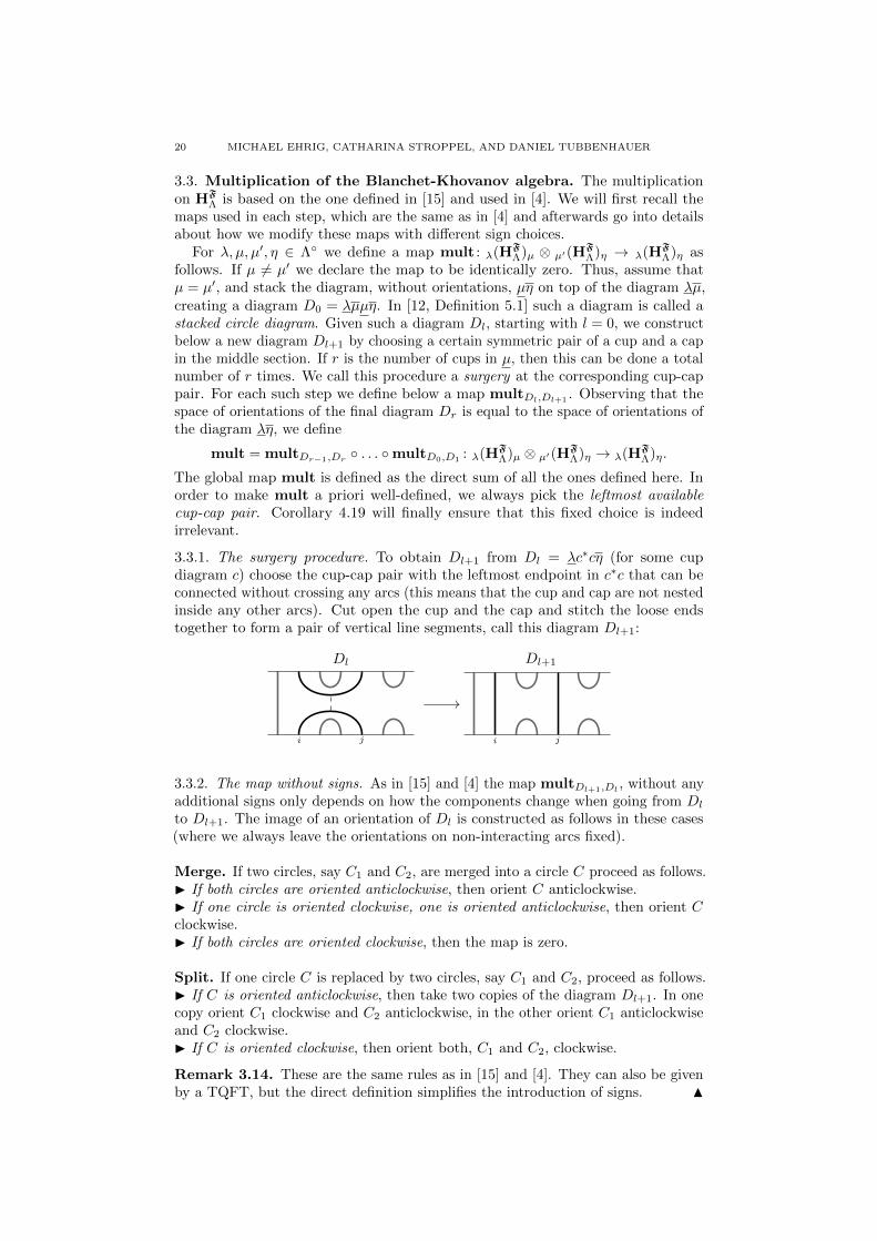
3.3.1. The surgery procedure. To obtain Dl+1 from Dl = λc∗cη (for some cupdiagram c) choose the cup-cap pair with the leftmost endpoint in c∗c that can beconnected without crossing any arcs (this means that the cup and cap are not nestedinside any other arcs). Cut open the cup and the cap and stitch the loose endstogether to form a pair of vertical line segments, call this diagram Dl+1:
ji
Dl
//
ji
Dl+1
3.3.2. The map without signs. As in [15] and [4] the map multDl+1,Dl, without any
additional signs only depends on how the components change when going from Dl
to Dl+1. The image of an orientation of Dl is constructed as follows in these cases(where we always leave the orientations on non-interacting arcs fixed).
Merge. If two circles, say C1 and C2, are merged into a circle C proceed as follows.I If both circles are oriented anticlockwise, then orient C anticlockwise.I If one circle is oriented clockwise, one is oriented anticlockwise, then orient Cclockwise.I If both circles are oriented clockwise, then the map is zero.
Split. If one circle C is replaced by two circles, say C1 and C2, proceed as follows.I If C is oriented anticlockwise, then take two copies of the diagram Dl+1. In onecopy orient C1 clockwise and C2 anticlockwise, in the other orient C1 anticlockwiseand C2 clockwise.I If C is oriented clockwise, then orient both, C1 and C2, clockwise.
Remark 3.14. These are the same rules as in [15] and [4]. They can also be givenby a TQFT, but the direct definition simplifies the introduction of signs. N

THE BLANCHET-KHOVANOV ALGEBRAS 21
3.3.3. The map with signs. In general, the formulas below include two types of signs.One type, which we call dot moving signs, also appear in [12], while the second,called topological signs and saddle signs, are topological in nature and more involved.These second types of signs will be given an interesting meaning in Subsection 4.5.The main difference to [12] will be that we distinguish whether the two circles, thatare merged together or split into, are nested in each other or not. Define
t(C) = (a choice of) a rightmost point in the circle C.
and let γ denote the cup in the cup-cap pair we use to perform the surgery procedurein this step connecting vertices i < j.
Non-nested Merge. The non-nested circles C1 and C2 are merged into C. Theonly case that is modified here is:I One circle oriented clockwise, one oriented anticlockwise. Let Ck (for k ∈ {1, 2})be the clockwise oriented circle and let γdot be a sequence of arcs in C connectingt(Ck) and t(C) (neither t(Ck), t(C) nor γdot are unique, but possible choices differin distance by 2, making the sign well-defined, see also [12, Lemma 5.7], and thus,the reader may choose any of these). Proceed as in Subsection 3.3.2 and multiplywith the dot moving sign
(24) (−1)dΛ(γdot).
Nested Merge. The nested circles C1 and C2 are merged into C. Denote by Cin
the inner of the two original circles. The cases are modified as follows.I Both circles oriented anticlockwise. Proceed as above, but multiply with
(25) − (−1)14 (dΛ(Cin)−2) · (−1)sΛ(γ).
I One circle oriented clockwise, one oriented anticlockwise. Again perform thesurgery procedure as described in Subsection 3.3.2 and multiply with
(−1)dΛ(γdot) · (−(−1)14 (dΛ(Cin)−2)) · (−1)sΛ(γ),
where γdot is defined as in (24).Non-nested Split. The circle C splits into the non-nested circles Ci, containingthe vertices at position i, and Cj , containing the vertices at position j. For bothorientations we introduce a dot moving sign as well as a saddle sign as follows.I C oriented anticlockwise. Use the map as in Subsection 3.3.2, but the copy whereCi is oriented clockwise is multiplied with
(−1)dΛ(γndoti ) · (−1)sΛ(γ),
while the one where Cj is oriented clockwise is multiplied with
−(−1)dΛ(γndotj ) · (−1)sΛ(γ).
Here γndoti and γndot
j are sequences of arcs connecting (i, 0) and t(Ci) inside Cirespectively (j, 0) and t(Cj) in Cj (ndot can be read as “newly created dot”).I C oriented clockwise. In this case multiply the result with
(−1)dΛ(γdot) · (−1)dΛ(γndoti ) · (−1)sΛ(γ).
Here γdot is a sequence of arcs connecting t(C) and t(Cj) in C and γndoti is as before.
Nested Split. We use here the same notations as in the non-nested split case aboveand furthermore denote by Cin the inner of the two circles Ci and Cj . The differenceto the non-nested case is that we substitute the saddle sign with a topological sign.

22 MICHAEL EHRIG, CATHARINA STROPPEL, AND DANIEL TUBBENHAUER
I C oriented anticlockwise. We use the map as defined in Subsection 3.3.2, but thecopy where Ci is oriented clockwise is multiplied with
(−1)dΛ(γndoti ) · (−1)
14 (dΛ(Cin)−2),
while the copy where Cj is oriented clockwise is multiplied with
−(−1)dΛ(γndotj ) · (−1)
14 (dΛ(Cin)−2).
Here γndoti and γndot
j are as before.I C oriented clockwise. We multiply with
(−1)dΛ(γdot) · (−1)dΛ(γndoti ) · (−1)
14 (dΛ(Cin)−2),
again with the same notations as above.
3.3.4. Examples for the multiplication. We give below examples for some of theshapes that can occur during the surgery procedure and determine the signs. In allexamples assume that outside of the shown strip all entries of the weights are ◦.
Example 3.15. This example illustrates the merge situation. First we look at asimple merge of two anticlockwise, non-nested circles. In this case no signs appearat all that means we have
∨ ∧∨ ∧
//
∨ ∧∨ ∧
// ∨ ∧(26)
The rightmost step above, called collapsing, is always performed at the end of amultiplication procedure and is omitted in what follows.
Secondly, we consider a merge of two anticlockwise, nested circles. Depending onthe concrete shape of the diagram it can produce different signs:
∨ ∧ ∨ ∧∨ ∨ ∧ ∧
//
∨ ∧ ∨ ∧∨ ∧ ∨ ∧
and
∨ ∨ ∧ ∧ ∨ ∧∨ ∨ ∧ ∨ ∧ ∧
// −∨ ∧ ∨ ∧ ∨ ∧∨ ∧ ∨ ∧ ∨ ∧
(27)
Note that, in contrast to [15], [4] or [12], nested merges can come with a sign. N
Example 3.16. This example illustrated the two versions of a split. In both cases anon-nested merge is performed, followed by a split into two non-nested respectivelynested circles. First, the H-shape:

THE BLANCHET-KHOVANOV ALGEBRAS 23
∨ ∧ ∨ ∧∨ ∧ ∨ ∧
//
∨ ∧ ∨ ∧∨ ∧ ∨ ∧
// −∨ ∧ ∧ ∨
∨ ∧ ∧ ∨−
∧ ∨ ∨ ∧
∧ ∨ ∨ ∧
∨ ∧ ∨ ∧
∧ ∨ ∧ ∨//∧ ∨ ∧ ∨
∧ ∨ ∧ ∨// −
∧ ∨ ∧ ∨
∧ ∨ ∧ ∨
(28)
Next, the C shape.
∨ ∧ ∨ ∧∨ ∧ ∨ ∧
//
∨ ∧ ∨ ∧∨ ∧ ∨ ∧
// −∧ ∨ ∧ ∨
∧ ∨ ∧ ∨+
∨ ∧ ∨ ∧∨ ∧ ∨ ∧
∨ ∧ ∨ ∧
∧ ∨ ∧ ∨//∧ ∨ ∧ ∨
∧ ∨ ∧ ∨//
∧ ∧ ∨ ∨
∧ ∧ ∨ ∨N
(29)
Remark 3.17. The Cshape cannot appear as long as we impose the choice of theorder of cup-cap pairs from left to right in the surgery procedure and it will not beneeded in the proof of Theorem 4.18. N
3.4. Bimodules for Blanchet-Khovanov algebras. To define HF-bimodules weneed further diagrams moving from one block Λ to another block Γ.
Fix two blocks Λ,Γ ∈ bl� such that seq(Λ) and seq(Γ) coincide except at positionsi and i+ 1. Following [5], a (Λ,Γ)-admissible matching (of type ±αi) is a diagram tinside R× [0, 1] consisting of vertical lines connecting (k, 0) with (k, 1) if we havethat seq(Λ)k = seq(Γ)k = F and, depending on the sign of αi, an arc at positions iand i+ 1 of the form
αi :
i
× F
F × ,
i
F ◦
◦ F ,
i
F F
◦ × ,
i
× ◦
F F
−αi :
i
F ×
× F ,
i
◦ F
F ◦ ,
i
F F
× ◦ ,
i
◦ ×F F
(30)
where we view seq(Λ) as decorating the integral points of R × {0} and seq(Γ) asdecorating the integral points of R× {1}. Again, the first two moves in each roware called rays, the third ones cups and the last ones caps.
For t a (Λ,Γ)-admissible matching, λ ∈ Λ, and µ ∈ Γ we say that λtµ is orientedif cups respectively caps connect one ∧ and one ∨ in λ respectively µ, and raysconnect the same symbols in λ and µ. For Λ = (Λ0, . . . ,Λr) a sequence of blocks

24 MICHAEL EHRIG, CATHARINA STROPPEL, AND DANIEL TUBBENHAUER
a Λ-admissible composite matching is a sequence of diagrams t = (t1, . . . , tr) suchthat tk is a (Λk−1,Λk)-admissible matching of some type. We view the sequence ofmatchings as being stacked on top of each other. A sequence of weights λi ∈ Λi suchthat λk−1tkλk is oriented for all k is an orientation of the Λ-admissible compositematching t. For short, we tend to drop the word admissible, since the only matchingswe consider are admissible. Moreover, if only start Λ = Λ0 and end Γ = Λr matter,then we call t short a (Λ,Γ)-composite matching.
We stress that Λ-composite matching can contain lines, in contrast to the diagramswe consider for HF
Λ and HF.
Example 3.18. Below is a (Λ0,Λ5)-composite matching. Assume that outside ofthe indicated areas all symbols of the block sequences are equal to ◦.
◦ F F F F F F ◦ ◦ Λ5t5
◦ F F F ◦ × F ◦ ◦ Λ4t4
◦ F F ◦ F × F ◦ ◦ Λ3t3
◦ F ◦ F F × F ◦ ◦ Λ2t2
◦ F ◦ F F F × ◦ ◦ Λ1t1
◦ F ◦ ×0
◦ F × ◦ ◦ Λ0
The types of the matchings are −α0, α2, α−1, α0, α1 (read from bottom to top). NWe now want to consider bimodules between Blanchet-Khovanov algebras for
different blocks, or said differently, bimodules for the algebra HF.We start by defining a basis of the underlying graded K-vector space. To a
Λ-composite matching t we again associate a set of diagrams from which to createa K-vector space (its elements are called stretched circle diagrams)
(31) B◦(Λ, t) =
λ(t,ν)µ
∣∣∣∣∣∣λ ∈ Λ◦0, µ ∈ Λ◦r , ν = (ν0, . . . , νr) with νi ∈ Λi,λν0 oriented, νrµ oriented,νi−1tiνi oriented for all 1 ≤ i ≤ r.
As before we obtain the set B(Λ, t) by allowing λ ∈ Λ0 and µ ∈ Λr in (31).
Example 3.19. Let Λ be the block with block sequence F F ◦ × at positions 0,1, 2, 3 and Γ the block with sequence F F F F at the same positions (both with◦ everywhere else) and assume both blocks are balanced. Then an example for a(Λ,Γ)-matching of type α1 is the third diagram in the first row of (30) denoted hereby t1. Taking this as our composite matching we obtain a graded K-vector space ofdimension 6 with basis consisting of
∨ ∧ ∨ ∧∨ ∧ ◦ ×
∨ ∧ ∧ ∨∨ ∧ ◦ ×
∧ ∨ ∨ ∧∧ ∨ ◦ ×
∧ ∨ ∧ ∨∧ ∨ ◦ ×
∨ ∧ ∨ ∧∨ ∧ ◦ ×
∧ ∨ ∧ ∨∧ ∨ ◦ ×
N
For a basis vector µ(t,ν)η denote by η↓ its downwards reduction. This is the capdiagram obtained by stacking the diagrams t1, . . . , tr, η on top of each other from left
THE BLANCHET-KHOVANOV ALGEBRAS 25
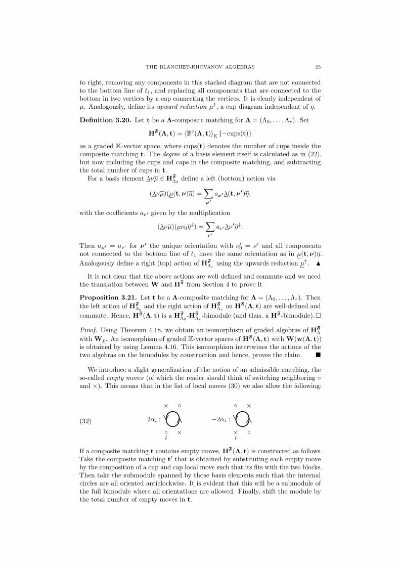
to right, removing any components in this stacked diagram that are not connectedto the bottom line of t1, and replacing all components that are connected to thebottom in two vertices by a cap connecting the vertices. It is clearly independent ofµ. Analogously, define its upward reduction µ↑, a cup diagram independent of η.
Definition 3.20. Let t be a Λ-composite matching for Λ = (Λ0, . . . ,Λr). Set
HF(Λ, t) = 〈B◦(Λ, t)〉K {−cups(t)}as a graded K-vector space, where cups(t) denotes the number of cups inside thecomposite matching t. The degree of a basis element itself is calculated as in (22),but now including the cups and caps in the composite matching, and subtractingthe total number of cups in t.
For a basis element λνµ ∈ HFΛ0
define a left (bottom) action via
(λνµ)(µ(t,ν)η) =∑ν′
aν′λ(t,ν′)η,
with the coefficients aν′ given by the multiplication
(λνµ)(µν0η↓) =
∑ν′
aν′λν′η↓.
Then aν′ = aν′ for ν′ the unique orientation with ν′0 = ν′ and all componentsnot connected to the bottom line of t1 have the same orientation as in µ(t,ν)η.
Analogously define a right (top) action of HFΛr
using the upwards reduction µ↑. N
It is not clear that the above actions are well-defined and commute and we needthe translation between W and HF from Section 4 to prove it.
Proposition 3.21. Let t be a Λ-composite matching for Λ = (Λ0, . . . ,Λr). Then
the left action of HFΛ0
and the right action of HFΛr
on HF(Λ, t) are well-defined and
commute. Hence, HF(Λ, t) is a HFΛ0
-HFΛr
-bimodule (and thus, a HF-bimodule).�
Proof. Using Theorem 4.18, we obtain an isomorphism of graded algebras of HFΛ
with W~k. An isomorphism of graded K-vector spaces of HF(Λ, t) with W(w(Λ, t))is obtained by using Lemma 4.16. This isomorphism intertwines the actions of thetwo algebras on the bimodules by construction and hence, proves the claim. �
We introduce a slight generalization of the notion of an admissible matching, theso-called empty moves (of which the reader should think of switching neighboring ◦and ×). This means that in the list of local moves (30) we also allow the following:
2αi :
i
× ◦∨ ∧◦ ×
−2αi :
i
×◦∨ ∧
◦×(32)
If a composite matching t contains empty moves, HF(Λ, t) is constructed as follows.Take the composite matching t′ that is obtained by substituting each empty moveby the composition of a cup and cap local move such that its fits with the two blocks.Then take the submodule spanned by those basis elements such that the internalcircles are all oriented anticlockwise. It is evident that this will be a submodule ofthe full bimodule where all orientations are allowed. Finally, shift the module bythe total number of empty moves in t.

26 MICHAEL EHRIG, CATHARINA STROPPEL, AND DANIEL TUBBENHAUER
Example 3.22. The pictures below are wildcards for the HF-bimodules definedvia the illustrated matchings.
× ◦
F F
◦ ×∼=
i
× ◦∨ ∧◦ ×
{+1} ⊕
i
× ◦∨ ∧◦ ×
{−1} ,
◦ ×F F
× ◦∼=
i
×◦∨ ∧
◦×{+1} ⊕
i
×◦∨ ∧
◦×{−1}
The isomorphisms of HF-bimodules are evident by the construction above. NProposition 3.23. The HF-bimodules HF(Λ, t) are finite-dimensional, graded
biprojective HF-bimodules. �Proof. Clearly, HF(Λ, t) are graded and finite-dimensional HF-bimodules. We onlyprove here projectivity for the left action, the right action is done analogously.Denote by Λ respectively Γ the first respectively last block in Λ. For any µ ∈ Γdenote by µ↓1µ↓ the idempotent in HF
Λ corresponding to the downwards reduction
of µ. Then, as an HFΛ-module, HF(Λ, t) decomposes as a direct sum of modules of
the form HFΛ · (µ↓1µ↓), which are projective HF
Λ-modules, proving the claim. �This proposition again motivates the definition of the following 2-category which
is, as before, one of the main objects that we are going to study.
Definition 3.24. Given HF as above, let HF-biModpgr be the following 2-category:
• Objects are the various Λ ∈ bl� together with a zero object.• 1-morphisms are finite sums and tensor products (taken over HF) of the
HF-bimodules HF(Λ, t).
• The composition HF-bimodules is given by tensoring (over HF).
• 2-morphisms are HF-bimodule homomorphisms.• The vertical composition of HF-bimodule homomorphisms is the usual
composition and the horizontal composition is given by tensoring (over HF).
We consider HF-biModpgr as a graded 2-category with 2-hom-spaces as in (1). N
In analogy to Definition 2.16, the objects and 1-morphisms in HF-biModpgr forma K-linear 1-category, which we denote by C.
4. Equivalences
In this section we assume that all appearing blocks Λ and ~k are balanced. Ourgoal now is to construct an isomorphism of graded algebras Φ : W◦ → HF (whereW◦ is a certain subalgebra of W defined in (39)). From this we obtain:
Theorem 4.1. There is an equivalence of graded, K-linear 2-categories
Φ : W-biModpgr
∼=−→ HF-biModpgr
induced by Φ under which the W-bimodules W(w(Λ, t)) (with w(Λ, t) defined in
Definition 4.9 below) are identified with the HF-bimodules HF(Λ, t). �4.1. Some useful lemmas. In order to prove Theorem 4.1, we need some lemmas.
Lemma 4.2. Let ` ∈ Z≥0. Then dimK(2EndF(12ω`)) = 1. �
Proof. Note that the identity foam on 12ω`(i.e. ` parallel phantom facets) is an
element of 2EndF(12ω`) which shows that dimK(2EndF(12ω`
)) ≥ 1. Now, given anyf ∈ 2EndF(12ω`
), denote by g ∈ 2EndF(∅) (where ∅ denotes the empty web) theclosed foam obtained from f by closings the ` bottom and top phantom facets tophantom spheres. Note that the question whether there are relations to reduce f to

THE BLANCHET-KHOVANOV ALGEBRAS 27
a scalar multiple of the identity foam on 12ω`is the same as the question whether g
can be evaluated to a scalar. But the latter can be achieved using the relations in F(which can be shown similar as in [16, Proposition 5]). Thus, every such f is a scalarmultiple of the identity foam on 12ω`
which shows that dimK(2EndF(12ω`)) ≤ 1. �
Lemma 4.3. The following foams are locally one-sided invertible in F (the ones inthe first column have a right inverse obtained by gluing from the bottom, the onesin the second a left inverse obtained by gluing from the top):
f1 =
•, f3 =
f2 = , f4 =
•
(33)
Similarly with the dots moved to the opposite facets. This implies locally that
2
2 f1
f2
//
2
2
{+1} ⊕
2
2
{−1}(−f3 f4
)//
2
2
(34)
are isomorphisms in W-biModpgr between web bimodules. �Proof. The statement of one-sided invertibility follows from the top bubble re-movals (11) (by stacking the foams in the first column on top of the foams in thesecond column). The invertibility of the foams with a different dot placement followsfrom the above and the dot migrations (15). The claim that the given morphismsare isomorphisms follows from composing them and using both bubble removals (11)and (12) as well as the neck cutting relation (13). �
The next lemmas say that isotopic webs give isomorphic web modules.
Lemma 4.4. We have locally
2
2
1
1
∼=
2
2
1
1
and
2
2
1
1
∼=
2
2
1
1
(35)
which are isomorphisms in W-biModpgr between web bimodules. �
28 MICHAEL EHRIG, CATHARINA STROPPEL, AND DANIEL TUBBENHAUER
Proof. The proof is similar to the one of Lemma 4.3: we can cap the bulge partrespectively cup the two straight lines using the evident (undotted) foams. Thenthe ordinary-to-phantom neck cutting relations (16) provide the isomorphisms. �Lemma 4.5. We have locally (where we use “rectangular” diagrams as in (17))
1 0
1 0
∼=
1 0
1 0
and
10
10
∼=
10
10
1 0 1 0
0 1 0 1
∼=
1 0 1 0
0 1 0 1
and
2 1 2 1
1 2 1 2
∼=
2 1 2 1
1 2 1 2
etc.
which are isomorphisms in W-biModpgr between web bimodules. Analogously forother isotopies of webs. �Proof. This is evident. �
Given a web u, then we denote by u the topological web obtained from u byforgetting orientations, labels and phantom edges, i.e. we have locally
1
1
7→ ,
2
2
7→ ∅ ,
2
1 1
7→ ,
2
1 1
7→
The topological webs are just non-crossing arcs and (closed) circles. We call any webu such that u is topologically a circle also just a circle. Similarly for webs u suchthat u is topologically a cup, cap or a line. Moreover, we assume that the leftmost
non-zero entries of Λ ∈ bl� and ~k ∈ bl� are at the same position in what follows.
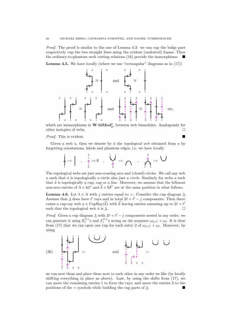
Lemma 4.6. Let λ ∈ Λ with j entries equal to ×. Consider the cup diagram λ.Assume that λ does have `′ rays and in total 2`+ `′ − j components. Then there
exists a cup-ray web u ∈ CupRay(~k) with ~k having entries summing up to 2`+ `′
such that the topological web u is λ. �Proof. Given a cup diagram λ with 2`+ `′ − j components nested in any order, we
can generate it using E(r)i ’s and F
(r)i ’s acting on the sequence ω`+`′ + ω`. It is clear
from (17) that we can open one cup for each entry 2 of ω`+`′ + ω`. Moreover, byusing
2 2 0 0
1 1 1 1
1 1 1 1
and
2 2 0 0
1 1 1 1
1 1 1 1
(36)
we can nest them and place them next to each other in any order we like (by locallyshifting everything in place as above). Last, by using the shifts from (17), wecan move the remaining entries 1 to form the rays, and move the entries 2 to thepositions of the × symbols while building the cup parts of λ. �

THE BLANCHET-KHOVANOV ALGEBRAS 29
Lemma 4.7. For each Λ-composite matching t, there exists a web u ∈ HomF(~k,~l)such that the topological web u is t. �
Proof. Mutatis mutandis as in the proof of Lemma 4.6. �
Even if we require a web u to be F -generated, there are still several ways to buildλ or t. In order to fix one, we say an F -generated web u prefers right to left if,inductively, the component with rightmost right boundary point of λ or t is createdfrom the rightmost available 2, if its a cup, or the rightmost available 1, if its aray (using a minimal number of possible moves). Moreover, we create the rightboundary point of a cup before the left. In the whole procedure we avoid creatingcircles.
Lemma 4.8. In the set-up of Lemma 4.6 or of Lemma 4.7 we can make u uniqueby requiring it to be F -generated and preferring right to left. �
Proof. An easy observation shows that we do not need E’s and E(2)’s in order tobuild λ or t (this holds more generally, see [32, Lemma 4.9]). Moreover, we can alwaysavoid creating circles. Thus, we obtain a set Fgen of F -generated webs such that ugives λ or t. All of these differ by distant commutation relations as in Lemma 4.5
(bottom moves) or Serre relations ΦWHowe((Fi+1F
(2)i − FiFi+1Fi + F
(2)i Fi+1)1~k) = 0.
One checks that, for fixed ~k ∈ bl�, all Serre relations have only two non-zero terms
and that the corresponding pictures are as in Lemmas 4.4 and 4.5. Hence, there isa unique web in Fgen that prefers right to left which can be shown by induction onthe number m of components of λ or t. This is clear if m = 0 or m = 1. For m > 1remove the leftmost connected component from λ or t and obtain λ′ or t′ with oneconnected component less. We can then apply the induction hypothesis and we geta unique web u′ such that u′ is λ′ or t′. Since we removed the leftmost componentof λ or of t, we can now just construct u from u′ (the result is unique due to ourconventions for such webs). �
Hence, the following definition makes sense.
Definition 4.9. Let Λ ∈ bl�. Given λ ∈ Λ, we denote by w(λ) the unique web asin Lemma 4.8, and given a Λ-composite matching t, we denote the unique web asin Lemma 4.8 by w(Λ, t). N
Examples of such webs are given in (36). Moreover, the following assignment
(37) ~k ∈ bl� 7→ Λ ∈ bl�, via 0 7→ ◦, 1 7→ F, 2 7→ ×,
clearly defines a bijection. Here ◦,F,× are entries of seq(Λ) and Λ is determineddemanding that Λ is balanced.
The next lemma is important for the calculation of the signs that turn up in themultiplication procedure. For this purpose, fix a circle C in a web w(λ)w(µ)∗ withcorresponding circle C ′ in λµ. For such a circle let nest(C) be the total number ofcircles C in
i nested in C. We denote by ipe(C) the total number of internal phantomedges of C (all such edges that lie in the interior of C, but not in the interior of anycircle nested in C) and more generally by
ipe(C −⋃nest(C)
i=1 C ini
)the total number of internal phantom edges of C after removing C in
i (by usingsimplifications as isotopies, (35) and (34)). Recalling d(·) from Definition 3.10, wehave:

30 MICHAEL EHRIG, CATHARINA STROPPEL, AND DANIEL TUBBENHAUER
Lemma 4.10. Given a circle diagram λµ (for suitable λ, µ ∈ Λ) and its associatedweb w(λ)w(µ)∗. Fix any circle C ′ in λµ and denote the associated circle inw(λ)w(µ)∗ by C. Then
ipe(C) = 14
(d(C ′) +
∑nest(C)i=1 d(Ciin)− 2 + 2 · nest(C)
),
ipe(C −⋃nest(C)
i=1 C ini
)= 1
4 (d(C ′)− 2) ,
where Ciin denotes the counterparts in λµ of the circles Ciin of w(λ)w(µ)∗.
Proof. We prove this by induction on the total length of all components in question.Circles C in their easiest form as on the left in (41) below have zero internal phantomedges and d(C) = 2, which is the start of our induction. The main observation nowis that the move in (35) increases the number of internal phantom edges by oneand the length by four (no matter which side of the diagram is the internal part ofthe circle). This shows the formulas in case that ipe(C) has no nested circles. Thegeneral formulas follow similarly, where we note that each × within C ′ increases itslength by 2 and creates a internal phantom edge in C. �
Example 4.11. The circles C ′ and C1in as on the right in (41) have d(C ′) = 6 and
d(C1in) = 2, and its counterpart C has one internal phantom edge after removing
the nested circle, while is has two internal phantom edges in total. Circles C ′ of Hor C shape as in (42) have d(C ′) = 6 respectively d(C ′) = 10 and their counterpartshave two respectively one internal phantom edge. N
4.2. The action of the quantum group Uq(gl∞) and arc diagrams. We obtainnow an action of the quantum group on C via the functor
ΦCHowe : Uq(gl∞)→ C,
given on objects by ΦCHowe(
~k) = Λ (with associated Λ ∈ bl� as in (37)) and onidentity morphisms by ΦC
Howe(1~k) = 1Λ. For the generating morphisms Ei1~k,
ΦCHowe(Ei1~k) is the bimodule corresponding to the unique local picture in the first
row of (30) that fits with Λ at position i and i + 1, or zero if none of them fits,ΦC
Howe(Fi1~k) is defined analogously using the local moves in the second row of (30).
The divided powers E(2)i 1~k respectively F
(2)i 1~k are sent to the bimodules for the
empty moves in (32) for 2αi respectively −2αi, again only if the block fits at positioni and i+ 1, and to zero otherwise. As in Subsection 2.3, all higher divided powers
E(r)i 1~k, F
(r)i 1~k for r > 2 are sent to zero.
By our discussion in the previous subsection, we see that ΦCHowe is a functor of
K-linear 1-categories.
4.3. The cup basis. The goal of this subsection is to define a basis on the side offoams which we call the cup basis.
Definition 4.12. Let u(W~k)v be as in Definition 2.23. Perform the following steps.
(I) Label each circle in uv∗ by either “no dot” or “dot”. Consider all possibilitiesof labeling the circles in such a way.
(II) For each such possibility we construct a foam f : 12ω`→ uv∗ via:
• If a circle is in its easiest form (i.e. only one incoming phantom edgeand only one outgoing phantom edge), then we locally use the foam atthe top right in (33) for circles with label “no dot” and the foam atthe bottom right in (33) for circles with label “dot”.• If a circle is more complicated, then we first apply the isomorphisms
described in Lemma 4.4 to reduce the circle to its easiest form, then weproceed as before, and finally we rebuild the circle using the inverses as

THE BLANCHET-KHOVANOV ALGEBRAS 31
in Lemma 4.4. Then we move the dot to the rightmost facet using (15)(the meticulous reader will note that this is ill-defined since there couldbe more than one rightmost facet, but one can choose any of them:dots passing from one rightmost facet to another always have to movean even number of times across phantom facets, see (35)).
From this we obtain a set of foams Cup(uv∗) which we call the cup basis of u(W~k)v.Basis elements of this basis are called basis cup foams. This name is justified: byconstruction, the foams in u(W~k)v are topological obtained by “cupping off circles
in the evident way”. Similarly, given u ∈ HomF(~k,~l) we can define a cup basisCup(u) of W(u) as above with the extra condition that we first close u in anypossible way. N
Lemma 4.13. Let u, v ∈ Cup(~k). The set Cup(uv∗) is a homogeneous, K-linearbasis of the space u(W~k)v. �Proof. That Cup(uv∗) is homogeneous is evident. To show that we get a basis, weuse induction on the number m of circles in uv∗. If m = 0, then the statementis clear by Lemma 4.2. So let m > 0. Choose now any maximally nested circleC (a circle that does not have any nested components) in uv∗ (we have to choosesuch a maximally nested circle in order use locally the foams from (33)). Remove itfrom uv∗ and obtain a new web uv∗ with fewer number of circles. By induction,Cup(uv∗) is a basis of u(W~k)v. Now apply the isomorphism from (34) and createa new circle by taking two copies of the basis elements from Cup(uv∗) (shifted upby one respectively down by one). The claim of the lemma follows if C was in itseasiest form. Otherwise, we rebuild the chosen circle C from the newly createdcircle using isomorphisms as
2
2
2
2
··· ··· ∼=
2
2
2
2
· · ·· · · ∼= etc.
from Lemma 4.4. Finally move dots to the rightmost facets using the dot migra-tions (15). Thus, the lemma also follows in this case. �
Lemma 4.14. Let u ∈ HomF(~k,~l). The set Cup(u) is a homogeneous, K-linearbasis of the web bimodule W(u). �Proof. Similar to the proof of Lemma 4.13: the induction start is the same and usesLemma 4.2. Note that W(u) is obtained from u (which has possibly only cups, capsand rays and no circles) by closing the bottom and top in any possible way. Thus,for each such “closure” of W(u) we can use the argument from above. �
We match the cup basis Cup(uv∗) with the basis λB◦(Λ)µ defined in (23).
Lemma 4.15. Let u, v be webs such that u = w(λ) and v = w(µ). There is anisomorphism of graded K-vector spaces
(38) Φλµuv : u(W~k)v → λ(HFΛ)µ
which sends Cup(uv∗) to λB◦(Λ)µ by identifying the cup foams without dots withanticlockwise circles and the foams with dots with clockwise circles. �

32 MICHAEL EHRIG, CATHARINA STROPPEL, AND DANIEL TUBBENHAUER
Proof. The sets Cup(uv∗) and λB◦(Λ)µ are clearly in bijective correspondence.Moreover, recalling Lemma 3.9 and the shift as in Definition 2.23, we obtain thatΦλµuv is homogeneous, which proves the lemma. �
Similarly, we match the cup basis Cup(u) with the basis B◦(Λ, t) from (31):
Lemma 4.16. Let u be a web such that u = w(Λ, t). There is an isomorphism ofgraded K-vector spaces
φλµuv : W(u)→ HF(Λ, t)
which sends Cup(u) to B◦(Λ, t) by identifying the basis cup foams without dotswith anticlockwise circles and the basis cup foams with dots with clockwise circles.�Proof. To show that (40) is indeed a homogeneous, K-linear isomorphism we canproceed as in the proof of Lemma 4.15 since both bases, Cup(u) and B◦(Λ, t), arein the end defined by closing u respectively t in all possible ways. �
Let still Λ ∈ bl�. Given λ, µ ∈ Λ, let us denote for u = w(λ) and v = w(µ) (andonly these)
(39) W◦(~k) =⊕
u,v∈Cup(~k)
u(W~k)v, W◦ =⊕~k∈bl
W~k.
The following is a direct consequence of Lemma 4.15.
Corollary 4.17. For any λ, µ ∈ Λ and u = w(λ), v = w(µ): the isomorphisms Φλµuvfrom (38) extend to isomorphisms of graded, K-vector spaces
(40) ΦΛ~k
: W◦~k→ HF
Λ, Φ : W◦ → HF.
where we identify ~k and Λ as in (37). �4.4. Proof of the main result. We deduce now Theorem 4.1 from the following.
Theorem 4.18. The maps from (40) are isomorphisms of graded algebras. �Before we prove Theorem 4.18 in Subsection 4.5, we deduce some consequences,
e.g. our main result. Moreover, the identification from Theorem 4.18 allows us touse topological arguments (i.e. foams) to deduce algebraic properties. In particular,we obtain the associativity of the Blanchet-Khovanov algebras.
Corollary 4.19. The multiplication rule from Subsection 3.3 is independent of theorder in which the surgeries are performed. This turns HF
Λ into a graded, associative,
unital algebra. Similar for (the locally unital) algebra HF. �Proof. This follows directly from Theorem 4.18 (note that the stated properties areclear if we work with the web algebra, see Corollary 2.27). �Remark 4.20. Theorem 4.18 leaves the question how the Blanchet-Khovanovalgebra HF
Λ and Khovanov’s original arc algebra Hm are related (and thus, how theBlanchet foam construction relates to the Khovanov [14] and Bar-Natan [1] theory
using cobordisms). On the other hand, the action of Uq(gln) from Subsection 4.2
extends to a 2-representation of Khovanov-Lauda’s categorification of Uq(gln),see [21, Proposition 3.3]. The same holds on the side of Khovanov’s arc algebra,
see [6, Remark 5.7]. Hence, it follows, for suitable choices of Λ and m, that HFΛ
and Hm are (graded) Morita equivalent. This can be deduced from Rouquier’suniversality theorem, see [28, Proposition 5.6 and Corollary 5.7], compare also to
[24, Proposition 5.18]. Since HFΛ and Hm are basic algebras, it follows by abstract
nonsense that HFΛ and Hm are isomorphic algebras (in fact, graded isomorphic
algebras). We stress however that it is not clear how such an isomorphism isconstructed explicitly. N

THE BLANCHET-KHOVANOV ALGEBRAS 33
Remark 4.21. Theorem 4.18 gives a way to compute the functorial chain complex(which is a link invariant) defined by Blanchet, see [2], and all its involved maps.
Indeed, in our framework HF comes equipped with an easy to handle basis andall appearing HF-module homomorphisms can explicitly be computed in this basis.This is in contrast to the local action used in [21, Proposition 3.3] to define Blanchet’slink homologies, see [21, Subsection 4.1], because it is not a priori clear in theirformulation how to do explicit computations (since globally a significant number ofnon-trivial signs come into play). N
Note that we consider webs in u ∈ Cup(~k) without imposing any relations. On the“uncategorified level” in the sense of Kuperberg [20], this has to be modified: denote
by Cup(~k)rel = Homrel(12ω,~k) the K-linear vector space obtained from Cup(~k) bymodding out by the circle removal relation
2
2
= (q + q−1) ·
2
2
and isotopy relations as in the Lemmas 4.4 and 4.5. Note that, on the “categorifiedlevel” in which we work in the rest of the paper, we do not need to impose theserelations since we “lift” them to the isomorphisms from Lemmas 4.3, 4.4 and 4.5.
Lemma 4.22. Let Λ ∈ bl� and ~k be its associated element in bl� (see (37)). Then
{u ∈ Cup(~k) | u = w(λ), λ ∈ Λ}is a K-linear basis of Cup(~k)rel.
Proof. This is clear by the relations imposed on Cup(~k)rel. �We are finally able to prove our main result.
Proof of Theorem 4.1. Instead of taking all webs u ∈ Cup(~k), it suffices to take a
basis of Cup(~k)rel and the webs w(λ) form such a basis by Lemma 4.22. Concretely,the algebras W~k (all webs) and W◦
~k(only basis webs) are graded Morita equivalent
(this can be seen similar to [23, Lemma 7.5]) and the statement follows fromTheorem 4.18. The identification of the bimodules as graded K-vector spaces isclear by Lemma 4.16, while the actions agree by Theorem 4.18 and construction ofthe actions. �4.5. The proof of the graded isomorphism. We now prove Theorem 4.18.
Proof of Theorem 4.18. By Lemma 4.15, it suffices to show that ΦΛ~k
is a homomor-
phism of algebras (since then so is Φ as well). For this purpose, fix λ, µ, ν ∈ Λ andset u = w(λ), v = w(µ), and w = w(ν). We show that any product of two basiscup foams f ∈ Cup(uv∗) and g ∈ Cup(vw∗) satisfies
Φλνuw(fg) = Φλµuv (f)Φµνvw(g)
(this is enough since all non-zero multiplications on side of HFΛ as well as on side of
W~k have to agree in the middle by definition).In order to do so, we show that each step in the multiplication procedure from
Definition 2.23 locally agrees with the one from Subsection 3.3. There are fourtopological different situations to check (compare with the cases in Subsection 3.3introducing the different signs):

34 MICHAEL EHRIG, CATHARINA STROPPEL, AND DANIEL TUBBENHAUER
(i) Non-nested Merge: two non-nested circles are replaced by one circle.(ii) Nested Merge: two nested circles are replaced by one circle.(iii) Non-nested Split: one circle is replaced by two non-nested circles.(iv) Nested Split: one circle is replaced by two nested circles.
We will consider these four cases step-by-step and compare the correspondingmultiplications rules. In addition to the four cases we will further distinguish thefollowing shapes of the involved underlying webs:
(A) Basic shape: the involved components are as small as possible with theminimal number of phantom facets.
(B) Minimal saddle: while the components themselves are allowed to be ofany shape, the involved saddle only includes a single phantom facet.
(C) General case: both, the shape as well as the saddle, are arbitrary.
We start by comparing the two multiplication rules for the basic shapes first.This will only involve simplified versions of the dot moving signs. The basic shapesfor (i), (ii), (iii) and (iv) are the following (with the multiplication step taking placein the marked region)
2
2
! and
2
2
2
2
!(41)
in cases (i) and (ii), and the H-shape and C-shape
2
2
2
2
! and
2
2
!(42)
in cases (iii) and (iv). Here we always display both, the web as well as its corre-sponding arc diagram.
I Non-nested merge - basic shape. In this case, we merge two simple cup webson the web side and two oriented circles on the arc diagram side. The followingtable gives the multiplication results in the four possible orientation combinations.
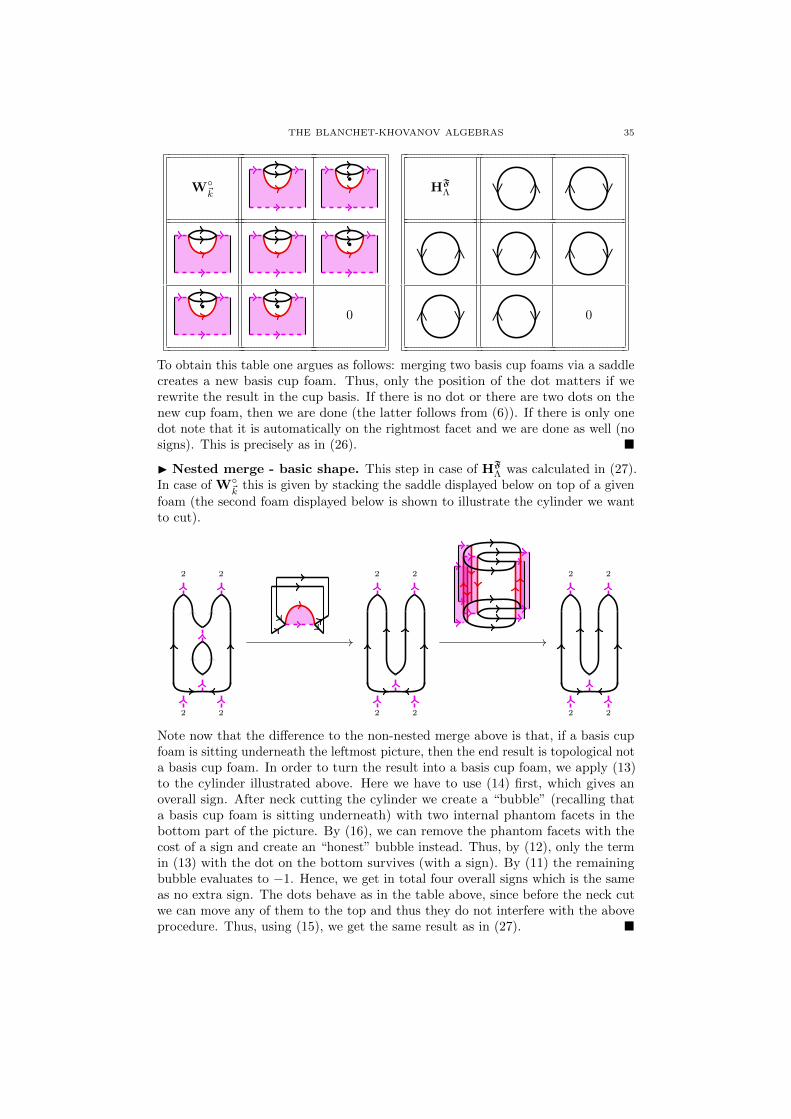
THE BLANCHET-KHOVANOV ALGEBRAS 35
W◦~k
•HF
Λ ∨ ∧ ∧ ∨
• ∨ ∧ ∨ ∧ ∧ ∨
• •0 ∧ ∨ ∧ ∨ 0
To obtain this table one argues as follows: merging two basis cup foams via a saddlecreates a new basis cup foam. Thus, only the position of the dot matters if werewrite the result in the cup basis. If there is no dot or there are two dots on thenew cup foam, then we are done (the latter follows from (6)). If there is only onedot note that it is automatically on the rightmost facet and we are done as well (nosigns). This is precisely as in (26). �
I Nested merge - basic shape. This step in case of HFΛ was calculated in (27).
In case of W◦~k
this is given by stacking the saddle displayed below on top of a given
foam (the second foam displayed below is shown to illustrate the cylinder we wantto cut).
2
2
2
2
//
2
2
2
2
//
2
2
2
2
Note now that the difference to the non-nested merge above is that, if a basis cupfoam is sitting underneath the leftmost picture, then the end result is topological nota basis cup foam. In order to turn the result into a basis cup foam, we apply (13)to the cylinder illustrated above. Here we have to use (14) first, which gives anoverall sign. After neck cutting the cylinder we create a “bubble” (recalling thata basis cup foam is sitting underneath) with two internal phantom facets in thebottom part of the picture. By (16), we can remove the phantom facets with thecost of a sign and create an “honest” bubble instead. Thus, by (12), only the termin (13) with the dot on the bottom survives (with a sign). By (11) the remainingbubble evaluates to −1. Hence, we get in total four overall signs which is the sameas no extra sign. The dots behave as in the table above, since before the neck cutwe can move any of them to the top and thus they do not interfere with the aboveprocedure. Thus, using (15), we get the same result as in (27). �
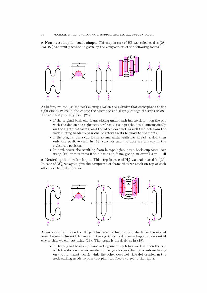
36 MICHAEL EHRIG, CATHARINA STROPPEL, AND DANIEL TUBBENHAUER
INon-nested split - basic shape. This step in case of HFΛ was calculated in (28).
For W◦~k
the multiplication is given by the composition of the following foams.
2
2
2
2
//
2
2
2
2
//
2
2
2
2
As before, we can use the neck cutting (13) on the cylinder that corresponds to theright circle (we could also choose the other one and slightly change the steps below).The result is precisely as in (28):
• If the original basis cup foams sitting underneath has no dots, then the onewith the dot on the rightmost circle gets no sign (the dot is automaticallyon the rightmost facet), and the other does not as well (the dot from theneck cutting needs to pass one phantom facets to move to the right).• If the original basis cup foams sitting underneath has already a dot, then
only the positive term in (13) survives and the dots are already in therightmost positions.• In both cases, the resulting foam is topological not a basis cup foam, but
using (16) once reduces it to a basis cup foam, giving an overall sign. �I Nested split - basic shape. This step in case of HF
Λ was calculated in (29).In case of W◦
~kwe again give the composite of foams that we stack on top of each
other for the multiplication.
2
2
//
2
2
//
2
2
Again we can apply neck cutting. This time to the internal cylinder in the secondfoam between the middle web and the rightmost web connecting the two nestedcircles that we can cut using (13). The result is precisely as in (29):
• If the original basis cup foams sitting underneath has no dots, then the onewith the dot on the non-nested circle gets a sign (the dot is automaticallyon the rightmost facet), while the other does not (the dot created in theneck cutting needs to pass two phantom facets to get to the right).

THE BLANCHET-KHOVANOV ALGEBRAS 37
• If the original basis cup foams sitting underneath has already a dot, thenonly the positive term in (13) survives and the dots are already in therightmost positions.• In both cases, the resulting foam is already topological a cup basis foam
and nothing needs to be done anymore. �All other situations (i.e. general shapes) are similar to the ones discussed, but
with the main difference that dots need to be shifted to the rightmost facets, someresults might not be in the topological form of a basis cup foam and one needs totake care of saddles with a possible number of additional internal phantom facets asin (20). These three facts together explain the signs turning up in the multiplicationdescribed in Subsection 3.3 with the first one corresponding to the dot moving signas in (24), the second corresponding to the topological signs as in (25) and the latterto the saddle sign as in (25).
Thus, we next deal with the minimal saddle situation as for example in (21). In
those cases s(γ) = 1 on the side of HFΛ. This will introduce the topological signs
and simplified versions (for s(γ) = 1) of the saddle signs.
I Non-nested merge - minimal saddle. This is topologically the same as innon-nested merge - basic shape, since the resulting foam will already be a basis cupfoam. Thus, the only sign comes from moving dots to the right which matches thedot moving sign turning up in the multiplication on the side of HF
Λ in (24). �I Nested merge - minimal saddle. Assume now that we merge a circle Cout
with some nested circle C in inside of it.The dot moving is as above in non-nested merge - minimal saddle and gives the
same sign as for HFΛ. The difference to the nested merge in the basic shape is that
we have to bring the resulting foam in the topological form of a basis cup foam. Tothis end, we can proceed as in nested merge - basic shape and cut the same cylinderas there. We first note that neither the dots which are already on the foam sittingunderneath nor the internal circles in Cout which are different from C in matter: wecan topologically move them “away from the local picture”.
Thus, to simplify a little bit, assume that C in is the only circle nested in Cout andthere are no dots. Following the procedure given as in nested merge - basic shapeabove, we see that the only things of importance are signs that come from cuttingthe cylinder with possible internal phantom facets and evaluating the “bubble” withpossible more than one internal phantom facets. Indeed, what matters is the numberof times we need to use (14) in the cutting procedure of the cylinder and the numberof times we need to use (16) in the bursting of the “bubble” (the rest stays thesame as before in nested merge - basic shape). Now, the number of times we needto apply (14) is ipe(Cout)− 1 (the −1 comes in because we apply a saddle whichremoves one of the internal phantom edges of the starting picture) and the numberof times we need to apply (16) is ipe(Cout − C in). By Lemma 4.10, we obtain that
(−1)ipe(Cout)−1+ipe(Cout−Cin) = (−1)14 (2(d(Cout)−2)+d(Cin)−2)
= −(−1)14 (d(Cin)−2) · (−1)1,
(43)
where Cout and Cin are the cup diagram counterparts of Cout and C in. Thisis precisely the same sign turning up on the side of HF
Λ (compare to (25) withsΛ(γ) = 1).
The case where Cout has several nested components, is similar since all nestedcomponents of Cout, which are not C in, increase the number of times we need touse (14) in the same way as the number of times we need to use (16) (hence, no
change modulo 2). Again, this matches the side of HFΛ in (25). �

38 MICHAEL EHRIG, CATHARINA STROPPEL, AND DANIEL TUBBENHAUER
I Non-nested split - minimal saddle. The dot moving is as before. Observenow that we do not have an extra sign turning up although the resulting foam isnot in the topological shape of a basis cup foam. To see this, we first simplify byassuming that the circle C which is split does not contain any nested components.Using the same cutting as in non-nested split - basic shape, we have signs comingfrom squeezing cylinders and simplifying “bubbles” (similar as above in nested merge- minimal saddle). But the number of times we need to apply (14) in this case isnow the same as the number of times one has to apply (16), namely ipe(C) − 1.Thus, again no change modulo 2. The case with nested components in C is nowanalogously as above in nested merge - minimal saddle since we can move dots andnested circles “away”. As before, this increases the number of times we need touse (14) in the same way as the number of times we need to use (16) (hence, no
change mod 2). Thus, we do not get an extra overall sign as in case of HFΛ (see
Subsection 3.3.3 non-nested split case). �I Nested split - minimal saddle. Moving dots is again as before. Furthermore,again, as in nested merge - minimal saddle, we need to topologically manipulatethe resulting foam until it is in basis cup foam shape. We can proceed as before innested split - basic shape and, similar as above in nested merge - minimal saddle,we pick up signs coming from cylinder cuts and bubble removals. In fact, the totalsign can be calculated analogously as in nested merge - minimal saddle (and is the
same as there). Again, this matches the side of HFΛ (see Subsection 3.3.3 nested
split case). �I Non-nested merge - general case. In fact, nothing changes compared to thediscussion in non-nested merge - minimal saddle, since dots passing a saddle alwayspass an odd number of phantom facets (compare to (20)) and the resulting foamsare topological already basis cup foams. �I Nested merge - general case. The dot moving stays as before. The only thingthat changes in contrast to nested merge - minimal saddle is that we obtain
(−1)ipe(Cout)−s+ipe(Cout−Cin) = (−1)14 (2(d(Cout)−2)+d(Cin)−2) · (−1)s(γ)−1
= −(−1)14 (d(Cin)−2) · (−1)s(γ).
within the topological re-writing procedure instead of the formula from (43). Thus,
this matches the side of HFΛ (see (25)). �
I Non-nested split - general case. Again, the dot moving stays as before.The difference to non-nested split - minimal saddle is that we have to apply (16)
s-times instead of once, which gives the sign turning up for HFΛ (see Subsection 3.3.3
non-nested split case). �I Nested split - general case. There is no difference to the arguments givenin nested split - minimal saddle. Again, this matches the side of HF
Λ (see Subsec-tion 3.3.3 nested split case). �Hence, in each case the topological multiplication agrees with the algebraicallydefined one. This concludes the proof. �
References
[1] D. Bar-Natan. Khovanov’s homology for tangles and cobordisms. Geom. Topol., 9:1443–1499,2005. URL: http://arxiv.org/abs/math/0410495, doi:10.2140/gt.2005.9.1443.
[2] C. Blanchet. An oriented model for Khovanov homology. J. Knot Theory Rami-fications, 19(2):291–312, 2010. URL: http://arxiv.org/abs/1405.7246, doi:10.1142/
S0218216510007863.

THE BLANCHET-KHOVANOV ALGEBRAS 39
[3] C. Blanchet, N. Habegger, G. Masbaum, and P. Vogel. Topological quantum field theories de-
rived from the Kauffman bracket. Topology, 34(4):883–927, 1995. doi:10.1016/0040-9383(94)
00051-4.[4] J. Brundan and C. Stroppel. Highest weight categories arising from Khovanov’s diagram
algebra I: cellularity. Mosc. Math. J., 11(4):685–722, 821–822, 2011. URL: http://arxiv.org/abs/0806.1532.
[5] J. Brundan and C. Stroppel. Highest weight categories arising from Khovanov’s diagram algebra
II: Koszulity. Transform. Groups, 15(1):1–45, 2010. URL: http://arxiv.org/abs/0806.3472,doi:10.1007/s00031-010-9079-4.
[6] J. Brundan and C. Stroppel. Highest weight categories arising from Khovanov’s diagram
algebra III: category O. Represent. Theory, 15:170–243, 2011. URL: http://arxiv.org/abs/0812.1090, doi:10.1090/S1088-4165-2011-00389-7.
[7] J. Brundan and C. Stroppel. Highest weight categories arising from Khovanov’s diagram
algebra IV: the general linear supergroup. J. Eur. Math. Soc. (JEMS), 14(2):373–419, 2012.URL: http://arxiv.org/abs/0907.2543, doi:10.4171/JEMS/306.
[8] J. Brundan and C. Stroppel. Gradings on walled Brauer algebras and Khovanov’s arc algebra.Adv. Math., 231(2):709–773, 2012. URL: http://arxiv.org/abs/1107.0999, doi:10.1016/j.
aim.2012.05.016.
[9] S. Cautis, J. Kamnitzer, and S. Morrison. Webs and quantum skew Howe duality.Math. Ann., 360(1-2):351–390, 2014. URL: http://arxiv.org/abs/1210.6437, doi:10.1007/
s00208-013-0984-4.
[10] D. Clark, S. Morrison, and K. Walker. Fixing the functoriality of Khovanov homology. Geom.Topol., 13(3):1499–1582, 2009. URL: http://arxiv.org/abs/math/0701339, doi:10.2140/gt.
2009.13.1499.
[11] M. Ehrig and C. Stroppel. 2-row Springer fibres and Khovanov diagram algebras for type D.To appear in Canad. J. Math. URL: http://arxiv.org/abs/1209.4998.
[12] M. Ehrig and C. Stroppel. Diagrammatic description for the categories of perverse sheaves onisotropic Grassmannians. URL: http://arxiv.org/abs/1306.4043.
[13] M. Jacobsson. An invariant of link cobordisms from Khovanov homology. Algebr. Geom.
Topol., 4:1211–1251 (electronic), 2004. URL: http://arxiv.org/abs/math/0206303, doi:10.2140/agt.2004.4.1211.
[14] M. Khovanov. A categorification of the Jones polynomial. Duke Math. J., 101(3):359–426,
2000. URL: http://arxiv.org/abs/math/9908171, doi:10.1215/S0012-7094-00-10131-7.[15] M. Khovanov. A functor-valued invariant of tangles. Algebr. Geom. Topol., 2:665–741, 2002.
URL: http://arxiv.org/abs/math/0103190, doi:10.2140/agt.2002.2.665.
[16] M. Khovanov. sl(3) link homology. Algebr. Geom. Topol., 4:1045–1081, 2004. URL: http://arxiv.org/abs/math/0304375, doi:10.2140/agt.2004.4.1045.
[17] M. Khovanov and A.D. Lauda. A categorification of quantum sln. Quantum Topol., 1(1):1–92,
2010. URL: http://arxiv.org/abs/0807.3250, doi:10.4171/QT/1.[18] M. Khovanov and L. Rozansky. Matrix factorizations and link homology. Fund. Math.,
199(1):1–91, 2008. URL: http://arxiv.org/abs/math/0401268, doi:10.4064/fm199-1-1.[19] J. Kock. Frobenius algebras and 2D topological quantum field theories, volume 59 of London
Mathematical Society Student Texts. Cambridge University Press, 2004.
[20] G. Kuperberg. Spiders for rank 2 Lie algebras. Comm. Math. Phys., 180(1):109–151, 1996.URL: http://arxiv.org/abs/q-alg/9712003.
[21] A.D. Lauda, H. Queffelec, and D.E.V. Rose. Khovanov homology is a skew Howe 2-representation of categorified quantum sl(m). To appear in Algebr. Geom. Topol. URL:http://arxiv.org/abs/1212.6076.
[22] G. Lusztig. Introduction to quantum groups. Modern Birkhauser Classics. Birkhauser/Springer,
New York, 2010. Reprint of the 1994 edition. doi:10.1007/978-0-8176-4717-9.[23] M. Mackaay. The sln-web algebras and dual canonical bases. J. Algebra, 409:54–100, 2014.
URL: http://arxiv.org/abs/1308.0566, doi:10.1016/j.jalgebra.2014.02.036.[24] M. Mackaay, W. Pan, and D. Tubbenhauer. The sl3-web algebra. Math. Z., 277(1-2):401–479,
2014. URL: http://arxiv.org/abs/1206.2118, doi:10.1007/s00209-013-1262-6.
[25] M. Mackaay, M. Stosic, and P. Vaz. slN -link homology (N ≥ 4) using foams and the Kapustin-Li formula. Geom. Topol., 13(2):1075–1128, 2009. URL: http://arxiv.org/abs/0708.2228,
doi:10.2140/gt.2009.13.1075.
[26] H. Queffelec and D.E.V. Rose. The sln foam 2-category: a combinatorial formulation ofKhovanov-Rozansky homology via categorical skew Howe duality. URL: http://arxiv.org/
abs/1405.5920.
[27] J. Rasmussen. Khovanov’s invariant for closed surfaces. URL: http://arxiv.org/abs/math/0502527.
[28] R. Rouquier. 2-Kac-Moody algebras. URL: http://arxiv.org/abs/0812.5023.

40 MICHAEL EHRIG, CATHARINA STROPPEL, AND DANIEL TUBBENHAUER
[29] A. Sartori. Categorification of tensor powers of the vector representation of Uq(gl(1|1)). To
appear in Selecta Math. (N.S.). URL: http://arxiv.org/abs/1305.6162.
[30] C. Stroppel. Tqft with corners and tilting functors in the Kac-Moody case. URL: http:
//arxiv.org/abs/math/0605103.
[31] D. Tubbenhauer. sl3-web bases, intermediate crystal bases and categorification. J. Al-gebraic Combin., 40(4):1001–1076, 2014. URL: http://arxiv.org/abs/1310.2779, doi:
10.1007/s10801-014-0518-5.
[32] D. Tubbenhauer. sln-webs, categorification and Khovanov-Rozansky homologies. URL: http://arxiv.org/abs/1404.5752.
M.E.: Mathematisches Institut, Universitat Bonn, Endenicher Allee 60, Room 1.003,53115 Bonn, Germany
E-mail address: [email protected]
C.S.: Mathematisches Institut, Universitat Bonn, Endenicher Allee 60, Room 4.007,53115 Bonn, Germany
E-mail address: [email protected]
D.T.: Mathematisches Institut, Universitat Bonn, Endenicher Allee 60, Room 1.003,53115 Bonn, Germany
E-mail address: [email protected]