The Black-Scholes Formula - Tim Worrall BLACK-SCHOLES investment is B 0 and write the rate of return...

ECO-30004 OPTIONS AND FUTURES SPRING 2008

The Black-Scholes Formula

The Black-Scholes Formula

We next examine the Black-Scholes formula for European options. The

Black-Scholes formula are complex as they are based on the geometric Brow-

nian motion assumption for the underlying asset price. Nevertheless they

can be interpreted and are easy to use once understood.

The payoff to a European call option with strike price K at the maturity

date T is

c(T ) = max[S(T )−K, 0]

where S(T ) is the price of the underlying asset at the maturity date. At

maturity if S(T ) > K the option to buy the underlying at K can be exercised

and the underlying asset immediately sold for S(T ) to give a net payoff of

S(T )−K. Since the option gives only the right and not the obligation to buy

the underlying asset, the option to buy the underlying will not be exercised

if doing so would lead to a loss, S(T ) −K < 0. The Black-Scholes formula

for the price of the call option at date t = 0 prior to maturity is given by

c(0) = S(0)N(d1)− e−rT KN(d2)

where N(d) is the cumulative probability distribution for a variable that has

a standard normal distribution with mean of zero and standard deviation of

one. It is the area under the standard normal density function from −∞ to

d and therefore gives the probability that a random draw from the standard

normal distribution will have a value less than or equal to d. We have there-

fore that 0 ≤ N(d) ≤ 1 with N(−∞) = 0,N(0) = 12

and N(+∞) = 1. The

term r is the continuously compounded risk-free rate of interest and d1 and

1

2 BLACK-SCHOLES

d2 satisfy

d1 =ln(S(0)

K) + (r + 1

2σ2)T

σ√

T

d2 = d1 − σ√

T =ln(S(0)

K) + (r − 1

2σ2)T

σ√

T

Here σ2 is the variance of the continuously compounded rate of return on the

underlying asset.

Likewise the payoff to a European put option with strike price K at the

maturity date T is

p(T ) = max[K − S(T ), 0]

as the put option gives the right to sell underlying asset at the strike price of

K. The Black-Scholes formula for the price of the put option at date t = 0

prior to maturity is given by

p(0) = c(0) + e−rT K − S(0) = e−rT K(1−N(d2))− S(0)(1−N(d1))

where d1 and d2 are defined above. By the symmetry of the standard normal

distribution N(−d) = (1−N(d)) so the formula for the put option is usually

written as

p(0) = e−rT KN(−d2)− S(0)N(−d1).

Assumptions Underlying the Black-Scholes Formula

To derive the Black-Scholes formula the following assumptions are required.

1. Markets are perfect: there are no transactions costs or taxes (i.e. there

is no bid-ask spread), assets can be short perfectly short sold and are

divisible (i.e. we can trade assets in negative and fractional units).

2. There is a risk-free asset and the interest rate on the risk-free asset is

unchanging over the life of the option.

ECO-30004 OPTIONS AND FUTURES 3

3. Trading is continuous .

4. The stock price follows a geometric Brownian motion process . That is

dS = µS dt + σS dz

where S is the stock price, µ is the expected return on the stock (as-

sumed to be unchanging over the life of the option) and σ is the stan-

dard deviation of the return on the stock (assumed to be unchanging

over the life of the option) and dz is a Wiener process .

We will explain a little bit more about assumptions 3 and 4 and how they

relate to the Black-Scholes formula.

Continuous Trading

We shall consider the effect of continuous trading on the risk-free asset first.

The assumption of continuous trading actually has many advantages mathe-

matically and makes the calculation of rates of return over different periods

rather easy.

The Rate of Return

The rate of return is simply the end value less the initial value as a proportion

of the initial value. Thus if 100 is invested and at the end value is 120 then

the rate of return is 120−100100

= 15

or 20%. If the the initial investment is BT−1

at time T − 1 and the end value is BT after one more period then the rate

of return is

r =BT −BT−1

BT−1

or equivalently the rate of return r satisfies BT = BT−1(1 + r). We can

generalise this to write the rate of return over T periods say when the initial

4 BLACK-SCHOLES

investment is B0 and write the rate of return as

r(T ) =BT −B0

B0

so that r(T ) satisfies BT = B0(1 + r(T )).

It is important to know the rate of return. However to compare rates

of return on different investments with different time horizons it is also im-

portant to have a measure of the rate of return per period. One method

of making this comparison is to to assume the asset is traded continuously

and can be priced by using the continuously compounded rates of return. To

explain this we first consider compound returns and then show what happens

when the compounding is continuous.

Compound Rates of Return

Compound interest rates are calculated by assuming that the principal (initial

investment) plus interest is re-invested each period. Compounding might be

done annually, semi-annually, quarterly, monthly or even daily. Assuming

the re-investment is done after each period, the per-period interest rate r on

the investment satisfies

(1 + r(T )) = (1 + r)T .

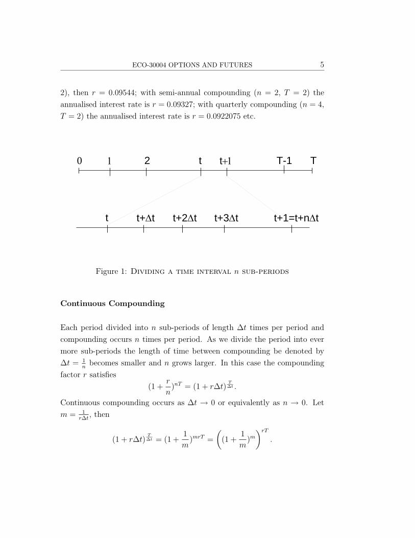
Now consider dividing up each period into n sub-periods each of length ∆t.

This is illustrated in Figure 1. Then if the compounding is done n times per

period, the compound interest rate r satisfies

(1 + r(T )) = (1 +r

n)nT .

For example consider a time period of one-year and suppose an investment

of 100 that yields 120 after two years (T = 2) has a rate of return r(2) = 0.2.

If the interest rate is annualised using annual compounding (n = 1, T =


2), then r = 0.09544; with semi-annual compounding (n = 2, T = 2) the

annualised interest rate is r = 0.09327; with quarterly compounding (n = 4,

T = 2) the annualised interest rate is r = 0.0922075 etc.

0 1 2 Tt+1t T-1

t t+Δt t+1=t+nΔtt+2Δt t+3Δt

Figure 1: Dividing a time interval n sub-periods

Continuous Compounding

Each period divided into n sub-periods of length ∆t times per period and

compounding occurs n times per period. As we divide the period into ever

more sub-periods the length of time between compounding be denoted by

∆t = 1n

becomes smaller and n grows larger. In this case the compounding

factor r satisfies

(1 +r

n)nT = (1 + r∆t)

T∆t .

Continuous compounding occurs as ∆t → 0 or equivalently as n → 0. Let

m = 1r∆t

, then

(1 + r∆t)T∆t = (1 +

1

m)mrT =

((1 +

1

m)m

)rT

.

6 BLACK-SCHOLES

As we let the interval between compounding ∆t go to zero then m → ∞.

The limit of (1 + 1m

)m as m→∞ is well known and is given by the formula

limm→∞

(1 +

1

m

)m

= e = 2.71828

where e = 2.7182818 is the base of the natural logarithm. Thus in the limit

the compounding factor is given by

(1 +r

n)nT =

((1 +

1

m)m

)rT

→ erT .

This gives a simple method for calculating the continuously compounded

rate of return r for any given investment. Suppose the initial outlay is B0

and the value of the portfolio or investment after T periods is BT . Then

since BT = B0(1 + r(T )) one has

BT

B0

= (1 + r(T )) = erT

so that taking logarithms of both sides

ln

(BT

B0

)= rT

or rewriting we have

r =1

Tln

(BT

B0

)=

1

T(ln BT − ln B0).

This is known as the continuously compounded rate of return.

The Continuously Compounded Rate of Return

The continuously compounded rate of return has the property that longer

period rates of return can be computed simply by adding shorter continuously

compounded rates of return. This is a very convenient feature which makes


using the continuously compounded rates of return especially simple. To see

this let rt denote the continuously compounded rate of return from period t

to t + 1, that is

rt = ln

(Bt+1

Bt

)where Bt is the value of the asset at time t. Let r(T ) denote the continuously

compounded rate of return over the period 0 to T ,

r(T ) = ln

(BT

B0

)= ln BT − ln B0.

Suppose that T = 2 then we can write this as

r(2) = ln B2 − ln B0 = (ln B2 − ln B1) + (ln B1 − ln B0) = r1 + r0.

Thus the continuously compounded rate of return over two periods is simply

the sum of the two period by period returns. In general for any value of T

we can write

r(T ) = (ln BT − ln BT−1) + (ln BT−1 − ln BT−2) + . . . + (ln B2 − ln B1) + (ln B1 − ln B0)

= rT−1 + rT−2 + . . . + r1 + r0 =T−1∑t=0

rt.

Thus the continuously compounded rate of return over time T is simply

the sum of the period by period returns. If rt is constant over time then

r(T ) = rT .

A Differential Equation

It will be useful to think about the value of the risk-free asset as it changes

over time. Let rt denote the rate of return between t and t + 1. Then over

any sub-interval of ∆t say between t and t + ∆t, rt satisfies

Bt+∆t = (1 + rt∆t)Bt.

8 BLACK-SCHOLES

Then taking the limit as ∆t→ 0 we have Bt+∆t−Bt → dB(t) where B(t) is

the price at time t and ∆t→ dt. Hence we can write

dB(t) = rtB(t)dt

or equivalentlydB(t)

B(t)= rtdt.

This is a differential equation. If we assume that rt = r is constant over time

(rt = r for each t) then this equation can be solved at by integration to give

the asset price at time T

ln BT − ln B0 == ln

(BT

B0

)= rT

or

BT = B0erT .

Geometric Brownian Motion

We have assumed so far that the rate of return was known so that we were

dealing with a risk-free asset. But for most assets the rate of return is uncer-

tain or stochastic. As the asset value also changes through time the we say

that the asset price follows a stochastic process. Fortunately the efficient

markets hypothesis provides some strong indication of what properties this

stochastic process will have.

A Coin Tossing Example

To examine the form that uncertain returns may take it is useful to think

first of a very simple stochastic process. This we have already seen as the

binomial model is itself a stochastic process. As an example consider the

case of tossing a fair coin where one unit is won if the coin ends up Heads


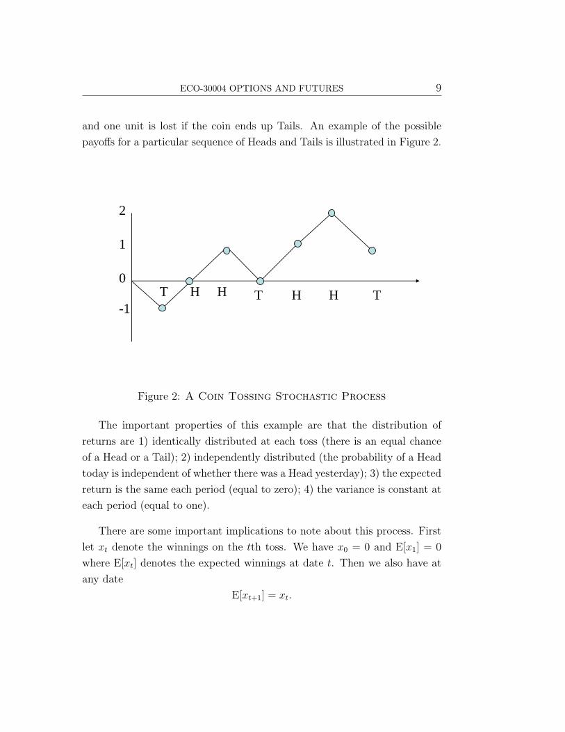
and one unit is lost if the coin ends up Tails. An example of the possible

payoffs for a particular sequence of Heads and Tails is illustrated in Figure 2.

2

1

-1

0T HH H H TT

Figure 2: A Coin Tossing Stochastic Process

The important properties of this example are that the distribution of

returns are 1) identically distributed at each toss (there is an equal chance

of a Head or a Tail); 2) independently distributed (the probability of a Head

today is independent of whether there was a Head yesterday); 3) the expected

return is the same each period (equal to zero); 4) the variance is constant at

each period (equal to one).

There are some important implications to note about this process. First

let xt denote the winnings on the tth toss. We have x0 = 0 and E[x1] = 0

where E[xt] denotes the expected winnings at date t. Then we also have at

any date

E[xt+1] = xt.

10 BLACK-SCHOLES

Any process with this property is said to be a martingale. Another impor-

tant property is that the variance of x is increasing proportionately to the

number of tosses. In particular letting σ2t denote the variance of the winnings

at the tth toss we have σ2t = t or in terms of the standard deviation (the

square root of the variance

σt =√

t.

This is illustrated in Figure 3. Figure 3 shows all possible winnings through

four tosses. The variance of winnings is easily calculated at each toss. For

example at the second toss the expected winnings are zero so the variance is

given by

σ22 =

1

4(2− 0)2 +

1

2(0− 0)2 +

1

4(−2− 0)2 = 1 + 1 = 2

and so the standard deviation is σ2 =√

2.

A Stochastic Process for Asset Prices

The efficient markets hypothesis implies that all relevant information is rapidly

assimilated into asset prices. Thus asset prices will respond only to new in-

formation (news) and since news is essentially unforecastable so to are asset

prices. The efficient market hypothesis also implies that it is impossible to

consistently make abnormal profits by trading on publicly available informa-

tion and in particular the past history of asset prices. Thus only the current

asset price is relevant in predicting future prices and past prices are irrele-

vant. This property is know as the Markov property for stock prices. If

we add a further assumption that the variability of asset prices is roughly

constant over time, then the asset price is said to follow a random walk.

This was true of our coin tossing example above.

Let ut denote the random rate of return from period t to t + 1. Then

St+1 = (1 + ut)St.


-1

12

0

-2-3

-1

1

3

-4

-2

0

2

4

0

σ2 = 1 σ2 = 2 σ2 = 4σ2 = 3

Figure 3: Coin Tossing Example: The Variance is Proportional

to Time

The return ut is now random because the future asset price is unknown.1

It can be considered as a random shock or disturbance. Taking natural

logarithm of both sides gives

ln(1 + ut) = ln St+1 − ln St.

Let ωt = ln(1 + ut). The ωt is the continuously compounded rate of return

from period t to t + 1. Since ut is random ωt will be random too. We shall

however assume

1. ωt are independently and identically distributed

1This was the case in our binomial model where ut takes on either the value of u inthe upstate or d in the down state.

12 BLACK-SCHOLES

2. ωt is normally distributed with a mean of ν and variance of σ2 (both

independent of time).2

With these assumptions we can see how the stock price is distributed at a

future date. Suppose we start from a given value S0, then

ln S1 = ln S0 + ln(1 + u0)

ln S2 = ln S1 + ln(1 + u1) = ln S0 + ln(1 + u0) + ln(1 + u1)

ln S3 = ln S2 + ln(1 + u2) = ln S0 + ln(1 + u0) + ln(1 + u1) + ln(1 + u2)

... =...

ln ST = ln S0 +T−1∑t=0

ln(1 + ut) = ln S0 +T−1∑t=0

ωt.

Since ωt is a random variable which is identically and independently dis-

tributed and such that the expected value E[ωt] = ν and variance Var[ωt] =

σ2 then taking expectations we have that ln ST is normally distributed such

that

E[ln ST ] = ln S0 + νT

and

Var[ln ST ] = σ2T.

Standard Normal Variable

We have seen that ln ST is normally distributed with mean (expected value)

of ln S0 + νT and variance of σ2T . It is useful to transform this to a variable

which has a standard normal distribution with mean of zero and standard

deviation of one. Such a variable is called a standard normal variable. To

2In fact when we take the limit there is no need to assume normality of the distributionas this will be guaranteed by the Central Limit Theorem.


make this transformation, we subtract the mean and divide by the standard

deviation (square root of the variance). Thus

ln ST − ln S0 − νT

σ√

T= −

ln(

S0

ST

)+ νT

σ√

T

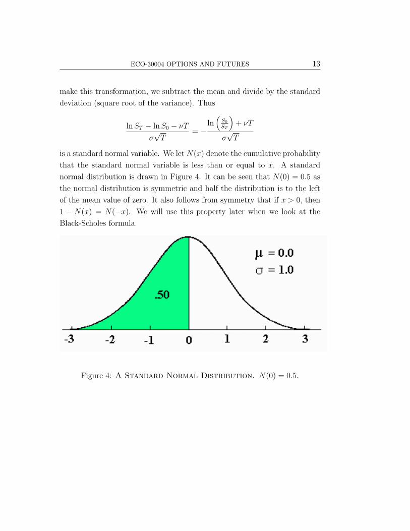
is a standard normal variable. We let N(x) denote the cumulative probability

that the standard normal variable is less than or equal to x. A standard

normal distribution is drawn in Figure 4. It can be seen that N(0) = 0.5 as

the normal distribution is symmetric and half the distribution is to the left

of the mean value of zero. It also follows from symmetry that if x > 0, then

1 − N(x) = N(−x). We will use this property later when we look at the

Black-Scholes formula.

Figure 4: A Standard Normal Distribution. N(0) = 0.5.

14 BLACK-SCHOLES

The Expected Rate of Return

Unfortunately, “the expected rate of return” is a rather ill-defined concept.

If we rewrite the above equation for ν we have

ν =1

T

(E

[ln

(ST

S0

)]).

This is known as the expected continuously compounded rate of return. That

is to say we look at the the continuously compounded rates of return and then

take expectations. However we can do it another way, which is to compute

the expected rates of return and then do our continuous compounding. This

would give us

µ =1

T

(ln

(E

[ST

S0

])).

Notice that the difference is that the Expectations operator appears inside

the logarithm. The value µ is know as the logarithm of expected return or

sometimes confusingly as the expected rate of return. The values of ν and µ

will be different if the asset is uncertain. Fortunately there is a very simple

relationship between ν and µ which is given by3

µ = ν +1

2σ2.

The reason why µ exceeds ν can be seen because the distribution of asset

prices is lognormal.

Lognormal Random Variable

Since the logarithm of the asset price is normally distributed the asset price

itself is said to be lognormally distributed. In practice when one looks at the

empirical evidence asset prices are reasonably closely lognormally distributed.

3The equation below always holds approximately and holds exactly in the limit.


We have assumed that that ωt = ln(1+ut) is normally distributed with an

expected value of ν and variance σ2. But 1+ut is a lognormal variable. Since

1 + ut = eωt we might guess that the expected value of ut is E[ut] = eν − 1.

However this would be WRONG. The expected value of ut is

E[ut] = eν+ 12σ2 − 1.

The expected value is actually higher than anticipated by half the variance.

The reason why can be seen from looking at an example of the lognormal

distribution which is drawn in Figure 5. The distribution is skewed and as

the variance increases the lognormal distribution will spread out. It cannot

spread out too much in a downward direction because the variable is always

non-negative. But it can spread out upwards and this tends to increase the

mean value. One can likewise show that the expected value of the asset price

at time T is

E[ST ] = S0e(ν+ 1

2σ2)T .

Hence

E[ST ] = s0eµT .

That is we “expect” the stock price to grow exponentially at the constant

rate µ. However our best forecast would be at a rate of ν and hence we

should in some sense always “expect less than the expected”.

Arithmetic and geometric rates of return

We now consider µ and ν again. Suppose we have an asset worth 100 and

for two successive periods it increases by 20%. Then the value at the end of

the first period is 120 and the value at the end of the second period is 144.

Now suppose that instead the asset increases in the first period by 30%

and in the second period by 10%. The average or arithmetic mean of the

return is 20%. However the value of the asset is 130 at the end of first period

16 BLACK-SCHOLES

0

0.1

0.2

0.3

0.4

0.5

0.6

0.7

0.8

0.9

1 6 11 16 21 26 31 36 41 46 51 56 61 66 71 76 81 86 91 96 101

106

111

116

121

126

131

136

141

146

151

156

Figure 5: A Lognormal Distribution

and 143 at the end of the second period. The variability of the return has

meant that the asset is worth less after two periods even though the average

return is the same. We can calculate the equivalent per period return that

would give the same value of 143 after two periods if there were no variance

in the returns. That is the value ν that satisfies

143 = 100(1 + ν)2.

This value is known as the geometric mean. It is another measure of the

average return over the two periods. Solving this equation gives the geometric

mean as ν = 0.195826 or 19.58% per period4 which is less than the arithmetic

rate of return per period.

4The geometric mean of two numbers a and b is√

ab. Thus strictly speaking 1 + g =1.195826 is the geometric mean of 1.1 and 1.3.


There is a simple relationship between the arithmetic mean return, the

geometric mean return and the variance of the return. Let µ1 = µ + σ be

the rate of return in the first period and let µ2 = µ− σ be the rate of return

in the second period. Here the average rate of return is 12(µ1 + µ2) = µ and

the variance of the two rates is σ2. The geometric rate of return µ satisfies

(1 + ν)2 = (1 + µ1)(1 + µ2). Substituting and expanding this gives

1 + 2ν + ν2 = (1 + µ + σ)(1 + µ− σ) = (1 + µ)2 − σ2 = 1 + 2µ + µ2 − σ2

or

ν = µ− 1

2σ2 +

1

2(µ2 − ν2).

Since rates of return are typically less than one, the square of the return is

even smaller and hence the difference between two squared percentage terms

is smaller still. Hence we have the approximation ν ≈ µ− 12σ2 or

geometric mean ≈ arithmetic mean− 1

2variance.

This approximation will be better the smaller are the interest rates and the

smaller is the variance. In the example µ = 0.2 and σ = 0.1 so 12σ2 = 0.005

and µ− 12σ2 = 0.1950 which is close to the actual geometric mean of 0.1958.

Thus the difference between µ and ν is that ν is the geometric rate of return

and µ is the arithmetic rate of return. It is quite usual to use the arithmetic

rate and therefore to write that the expected value of the logarithm of the

stock price satisfies

E[ln ST ] = ln S0 +

(µ− 1

2σ2

)T

and

Var[ln ST ] = σ2T.

18 BLACK-SCHOLES

The Continuous Trading Limit5

This section examines what happens in the limit as the stock price can change

continuously and randomly. This section is mathematically more demanding

and therefore can largely be ignored. The important result is that with

continuous trading the asset price follows a stochastic differential equation

given by

dS(t) = µS(t) dt + σS(s) dz.

where dz is a Weiener process which is described in the next section. This

process for stock prices is known as geometric Brownian motion and shows

that the stock price consists of two components. Firstly a deterministic

component which shows the stock price growing at a rate of µ and secondly

a random or disturbance component with a volatility of σ.

A Wiener Process

Consider a variable z which takes on values at discrete points in time t =

0, 1, . . . , T and suppose that z evolves according to the following rule:

zt+1 = zt + ε; W0 fixed

where ε is a random drawing from a standardized normal distribution, that

is with mean of zero and variance of one. The draws are assumed to be in-

dependently distributed. This represents a random walk where on average

z remains unchanged each period but where the standard deviation of the

realized value is one each period. At date t = 0, we have E[zT ] = z0 and the

variance V ar[zT ] = T as the draws are independent.

Now divide the periods into n subperiods each of length ∆t. To keep the

process equivalent the variance in the shock must also be reduced so that

5This section can be considered optional.


the standard deviation is√

∆t. The resulting process is known as a Wiener

process. The Wiener process has two important properties:

Property 1 The change in z over a small interval of time satisfies:

zt+h = zt + ε√

∆t.

Then as of time t = 0, it is still the case that E[zT ] = z0 and the

variance V ar[zT ] = T . This relation may be written

∆z(t + ∆t) = ε√

∆t

where ∆z(t + ∆t) = zt+∆t− zt. This has an expected value of zero and

standard deviation of√

∆t.

Property 2 The values of ∆z for any two different short intervals of time

are independent.

It follows from this that

z(T )− z(0) =N∑i

εi

√∆t

where N = T/∆t is the number of time intervals between 0 and T . Hence

we have

E[Z(T )] = z(0)

and

Var[z(T )] = N∆t = T

or the standard deviation of z(T ) is√

T .

Now consider what happens in the limit as ∆t→ 0, that is as the length

of the interval becomes an infinitesimal dt. We replace ∆z(t + ∆t) by dz(t)

which has a mean of zero and standard deviation of dt. This continuous

time stochastic process is also known as Brownian Motion after its use in

20 BLACK-SCHOLES

physics to describe the motion of particles subject to a large number of small

molecular shocks.

This process is easily generalized to allow for a non-zero mean and arbi-

trary standard deviation. A generalized Wiener process for a variable x

is defined in terms of dz(t) as follows

dx = a dt + b dz

where a and b are constants. This formula for the change in the value of x

consists of two components, a deterministic component a dt and a stochastic

component b dz(t). The deterministic component is dx = a dt or dxdt

= a

which shows that x = x0 + at so that a is simply the trend term for x.

Thus the increase in the value of x over one time period is a. The stochastic

component b dz(t) adds noise or variability to the path for x. The amount of

variability added is b times the Wiener process. Since the Wiener process has

a standard deviation of one the generalized process has a standard deviation

of b.

The Asset Price Process

Remember that we have

ln St+1 − ln St = ωt

where ωt is are independent random variables with mean ν and standard

deviation of σ. The continuous time version of this equation is therefore

d ln S(t) = ν dt + σ dz

where z is a standard Wiener process. The right-hand-side of the equation is

just a random variable that is evolving through time. The term ν is called the

drift parameter and the standard deviation of the continuously compounded

rate of return is√

Var[r(t)] = σ√

∆t and the term σ is referred to as the

volatility of the asset return.


Ito Calculus

We have written the process in terms of ln S(t) rather than S(t) itself. This

is convenient and shows the connection to the binomial model. However it is

usual to think in terms of S(t) itself too. In ordinary calculus we know that

d ln S(t) =dS(t)

S(t).

Thus we might think that dS(t)/S(t) = ν dt + σ dz. But this would be

WRONG. The correct version is

dS(t)

S(t)=

(ν +

1

2σ2

)dt + σ dz.

This is a special case of Ito’s lemma. Ito’s lemma shows that for any process

of the form

dx = a(x, t)dt + b(x, t)dz

then the function G(x, t) follows the process

dG =

(∂G

∂xa(x, t) +

∂G

∂t+

1

2

∂2G

∂x2b2(x, t)

)dt +

∂G

∂xb(x, t)dz.

We’ll see how to use Ito’s lemma. We have

d ln S(t) = ν dt + σ dz.

Then let ln S(t) = x(t), so s(T ) = G(x, t) = ex. Then upon differentiating

∂G

∂x= ex = S,

∂2G

∂S2= ex = S,

∂G

∂t= 0.

Hence using Ito’s lemma

dS(t) = (νS(t) + 0 +1

2σ2S(t))dt + σS(t) dz

or

dS(t) = (ν +1

2σ2)S(t) dt + σS(t) dz

22 BLACK-SCHOLES

Since µ = ν + 12σ2 we can write this as

dS(t) = µS(t) dt + σS(s) dz.

This process is know as geometric Brownian motion as it is the rate of change

which is Brownian motion. Thus sometimes the above equation is written as

dS(t)

S(t)= µ dt + σ dz.

Interpretation of the Black-Scholes Formula

After this rather long digression we return to the Black-Scholes formula

S(T )−K < 0. The Black-Scholes formula for the price of the call option at

date t = 0 prior to maturity is given by

c(0) = S(0)N(d1)− e−rT KN(d2)

where d1 and d2 satisfy

d1 =ln(S(0)

K) + (r + 1

2σ2)T

σ√

T

d2 = d1 − σ√

T =ln(S(0)

K) + (r − 1

2σ2)T

σ√

T

We need to be able to explain and interpret this formula.

Evaluating the Discounted Value of the Future Payoff (Using Risk-

Neutral Valuation)

Rewrite the Black-Scholes formula as

c(0) = e−rT(S(0)erT N(d1)−KN(d2)

).

The formula can be interpreted as follows. If the call option is exercised at

the maturity date then the holder gets the stock worth S(T ) but has to pay


the strike price K. But this exchange takes place only if the call finishes in

the money. Thus S(0)erT N(d1) represents the future value of the underlying

asset conditional on the end stock value S(T ) being greater than the strike

price K. The second term in the brackets KN(d2) is the present value of the

known payment K times the probability that the strike price will be paid

N(d2). The terms inside the brackets are discounted by the risk-free rate r

to bring the payments into present value terms. Thus the evaluation inside

the brackets is made using the risk-neutral or martingale probabilities and

N(d2) represents the probability that the call finishes in the money recall in

a risk neutral world.

Remember that in a risk-neutral world all assets earn the risk-free rate.

we are assuming the the logarithm of the stock price is normally distributed.

Thus ν the expected continuously compounded rate of return in a risk neutral

world is equal to r − 12σ2 where the variance is deducted to calculate the

certainty equivalent rate of return. Therefore at time T ln S(T ) is normally

distributed with a mean value of ln S(0)+(r− 12σ2)T and a standard deviation

of σ√

T . Thusln S(T )− (ln S(0)) + (r − 1

2σ2)T )

σ√

T

is a standard normal variable. The probability that S(T ) < K is therefore

given by N(−d2) and the probability that S(T ) > K is given by 1−N(−d2) =

N(d2).

It is more complicated to show that S(0)erT N(d1) is the future value of

underlying asset in a risk-neutral world conditional on S(T ) > K but a proof

can be found in more advanced textbooks.

24 BLACK-SCHOLES

The Replicating Portfolio

The formula also has another useful interpretation. From our analysis of the

binomial model we know that the value of the call is

c(0) = S(0)∆−B

where ∆ is the amount of the underlying asset bought and B is the amount

of money borrowed needed to synthesize the call option. From the for-

mula therefore N(d1) is the hedge parameter indicating the number of shares

bought and e−rT KN(d2) indicates the amount of cash borrowed to part fi-

nance the share purchase. Since 0 ≤ N(d) ≤ 1 the formula shows that

the replicating portfolio consists of a fraction of the underlying asset and a

positive amount of cash borrowed. The ∆ of this formula is also found by

partially differentiating the call price formula

∂c(0)

∂S(0)= ∆.

It is the slope of the curve relating the option price with the price of the

underlying asset. The cost of buying ∆ units of the stock and writing one

call option is S(0)∆− c(0). This portfolio is said to be delta neutral as a

small change in the stock price will not affect the value of the portfolio.

Boundary Conditions

A boundary condition tells us the price of the put or call at some extreme

value. Thus for example if we have a call option which is just about to expire,

then the value of the option must just be its intrinsic value max[S(T )−K, 0],

as the option has no time value left. If the Black-Scholes formula is correct

it must reduce to the intrinsic value when the time to maturity left is very


small. That is c(0) → max[S(0) − K, 0] as T → 0.6 We will chck that the

boundary conditions are indeed satisfied.

Boundary Conditions for a Call Option

We shall consider the boundary conditions for the call option. Consider first

the boundary condition for the call at expiration when T = 0. To do this

consider the formula for the call option as T → 0, that is as the time until

maturity goes to zero. At maturity c(T ) = max[S(T ) −K, 0] so we need to

show that as T → 0 the formula converges to c(0) = max[S(0) − K, 0]. If

S(0) > K then ln(S(0)K

) > 0 so that as T → 0, d1 and d2 → +∞. Thus N(d1)

and N(d2) → 1. Since e−rT → 1 as T → 0 we have that c(0) → S(0) − K

if S(0) > K. Alternatively if S(0) < K then ln(S(0)K

) < 0 so that as T → 0,

d1 and d2 → −∞ and hence N(d1) and N(d2) → 0. Thus c(0) → 0 if

S(0) < K. This is precisely as expected. If the option is in the money at

maturity, S(0) > K, it is exercised for a profit of S(0)−K and if it is out of

the money, S(0) < K, the option expires unexercised and valueless.

As another example consider what happens as σ → 0. In this case the

underlying asset becomes riskless so grows at the constant rate of r. Thus

the future value of the stock is S(T ) = erT S(0) and the payoff to the call

option at maturity is max[erT S(0)−K, 0]. Thus the value of the call at date

t = 0 is max[S(0)− e−rT K, 0]. To see this from the formula first consider the

case where S(0) − e−rT K > 0 or ln(S(0)K

) + rT > 0. Then as σ → 0, d1 and

d2 → +∞ and hence N(d1) and N(d2) → 1. Thus c(0) → S(0) − e−rT K.

Likewise when S(0)− e−rT K < 0 or ln(S(0)K

)+ rT < 0 then d1 and d2 → −∞as σ → 0. Hence N(d1) and N(d2) → 0 and so c(0) → 0. Thus combining

both conditions c(0)→ max[erT S(0)−K, 0] as σ → 0.

6In fact the Black-Scholes formula is usually derived by computing the process the calloption price must follow and imposing the boundary conditions.

26 BLACK-SCHOLES

Boundary Conditions for a Put Option

For a put option p(T ) = max[K − S(T ), 0] so we need to show that as

T → 0 the formula converges to p(0) = max[K − S(0), 0]. If S(0) > K

then ln(S(0)K

) > 0 so that as T → 0, d1 and d2 → +∞. Thus N(−d1)

and N(−d2) → 0. Since e−rT → 1 as T → 0 we have that p(0) → 0 if

S(0) > K. Alternatively if S(0) < K then ln(S(0)K

) < 0 so that as T → 0,

d1 and d2 → −∞ and hence N(−d1) and N(−d2) → 1. Since e−rT → 1

as T → 0 we have that p(0) → K − S(0) if S(0) < K This is precisely as

expected. If the option is in the money at now (at the maturity date T = 0)

and S(0) < K, it is exercised for a profit of K − S(0) and if it is out of the

money, S(0) > K, the option expires unexercised and valueless.

Now consider what happens to the put option as σ → 0. In this case the

underlying asset becomes riskless so grows at the constant rate of r. Thus the

future value of the stock is S(T ) = erT S(0) and the payoff to the put option

at maturity is max[K − erT S(0), 0]. Thus the value of the put at date t = 0

is max[e−rT K − S(0), 0] (that is discounting by the factor e−rT . To see this

from the formula first consider the case where e−rT K − S(0) > 0 or taking

logs and rearranging ln(S(0)K

) + rT < 0. Then as σ → 0, d1 and d2 → −∞and hence N(−d1) and N(−d2)→ 1. Thus p(0)→ e−rT K − S(0). Likewise

when e−rT K − S(0) < 0 or ln(S(0)K

) + rT > 0 then d1 and d2 → +∞ as

σ → 0. Hence N(−d1) and N(−d2) → 0 and so p(0) → 0. Thus combining

both conditions p(0)→ max[erT K − S(0), 0] as σ → 0.

The Black-Scholes Formula - Tim Worrall BLACK-SCHOLES investment is B 0 and write the rate of return...

Documents

Transcript of The Black-Scholes Formula - Tim Worrall BLACK-SCHOLES investment is B 0 and write the rate of return...