The Banking Panics in the United States in the 1930s: … Abstract “The Lessons from the Banking...

1

The Lessons from the Banking Panics in the United States in the

1930s for the Financial Crisis of 2007-2008

Michael Bordo

Department of Economics

Rutgers University

and NBER

[email protected]

and

John Landon Lane

Department of Economics

Rutgers University

[email protected]

.

Paper prepared for a seminar at the Graduate Center, CUNY, Feb 7, 2012.

mailto:[email protected]


2

Abstract

“The Lessons from the Banking Panics in the United States in the 1930s for the Financial

Crisis of 2007-2008”

In this paper we revisit the debate over the role of the banking panics in 1930-33 in

precipitating the Great Contraction. The issue hinges over whether the panics were

illiquidity shocks and hence (in support of Friedman and Schwartz (1963) greatly

exacerbated the recession which had begun in 1929, or whether they largely reflected

insolvency in response to the recession caused by other forces. Based on a VAR and new

data on the sources of bank failures in the 1930s from Richardson (2007), we find that

illiquidity shocks played a key role in explaining the bank failures during the Friedman

and Schwartz banking panic windows.

In the recent crisis the Federal Reserve learned the Friedman and Schwartz lesson from

the banking panics of the 1930s of conducting expansionary open market policy to meet

demands for liquidity. Unlike the 1930s the deepest problem of the recent crisis was not

illiquidity but insolvency and especially the fear of insolvency of counterparties.

Michael Bordo John Landon Lane

Department of Economics Department of Economics

Rutgers University Rutgers University

[email protected] [email protected]

Keywords: Banking Panics, Financial Crises, Monetary Policy

JEL: E52 N12



3

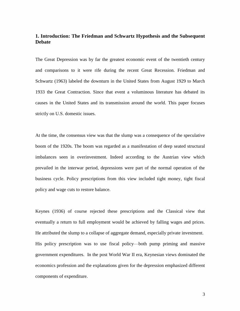
1. Introduction: The Friedman and Schwartz Hypothesis and the Subsequent

Debate

The Great Depression was by far the greatest economic event of the twentieth century

and comparisons to it were rife during the recent Great Recession. Friedman and

Schwartz (1963) labeled the downturn in the United States from August 1929 to March

1933 the Great Contraction. Since that event a voluminous literature has debated its

causes in the United States and its transmission around the world. This paper focuses

strictly on U.S. domestic issues.

At the time, the consensus view was that the slump was a consequence of the speculative

boom of the 1920s. The boom was regarded as a manifestation of deep seated structural

imbalances seen in overinvestment. Indeed according to the Austrian view which

prevailed in the interwar period, depressions were part of the normal operation of the

business cycle. Policy prescriptions from this view included tight money, tight fiscal

policy and wage cuts to restore balance.

Keynes (1936) of course rejected these prescriptions and the Classical view that

eventually a return to full employment would be achieved by falling wages and prices.

He attributed the slump to a collapse of aggregate demand, especially private investment.

His policy prescription was to use fiscal policy—both pump priming and massive

government expenditures. In the post World War II era, Keynesian views dominated the

economics profession and the explanations given for the depression emphasized different

components of expenditure.

4

Milton Friedman and Anna Schwartz in A Monetary History of the United States (1963)

challenged this view and attributed the Great Contraction from 1929 to 1933 to a collapse

of the money supply by one third brought about by a failure of Federal Reserve policy.

The story they tell begins with the Fed tightening policy in early 1928 to stem the Wall

Street boom. Fed officials believing in the real bills doctrine were concerned that the

asset price boom would lead to inflation. The subsequent downturn beginning in August

1929 was soon followed by the stock market crash in October. Friedman and Schwartz,

unlike Galbraith (1955), did not view the Crash as the cause of the subsequent depression.

They saw it as an exacerbating factor (whereby adverse expectations led the public to

attempt to increase their liquidity) in the decline in activity in the first year of the

Contraction.

The real problem arose with a series of four banking panics beginning in October 1930

and ending with Roosevelt’s national banking holiday in March 1933. According to

Friedman and Schwartz, the banking panics worked through the money multiplier to

reduce the money stock (via a decrease in the public’s deposit to currency ratio). The

panic in turn reflected what Friedman and Schwartz called a ‘ contagion of fear” as the

public fearful of being last in line to convert their deposits into currency, staged runs on

the banking system, leading to massive bank failures. In today’s terms it would be a

“liquidity shock”. The collapse in money supply in turn led to a decline in spending and,

in the face of nominal rigidities, especially of sticky money wages, a decline in

employment and output. The process was aggravated by banks dumping their earning

5

assets in a fire sale and by debt deflation. Both forces reduced the value of banks

collateral and weakened their balance sheets, in turn leading to weakening and insolvency

of banks with initially sound assets.

According to Friedman and Schwartz, had the Fed acted as a proper lender of last resort

as it was established to be in the Federal Reserve Act of 1913 that it would have offset

the effects of the banking panics on the money stock and prevented the Great Contraction.

Friedman and Schwartz’s “money hypothesis “was attacked by Peter Temin in Did

Monetary Forces Cause the Great Depression? (1976). Temin challenged Friedman and

Schwartz’s assumption that the money supply collapse was an exogenous event. He

argued that money supply fell in response to the downturn. He attributed the collapse in

income to a decline in autonomous consumption expenditure and in exports. The fall in

income in turn reduced the demand for money and money supply responded. At the heart

of his critique is the view that the banking collapses beginning in October of 1930 were

not “contagious liquidity shocks” but endogenous “insolvency” responses to a previous

decline in economic activity especially in agricultural regions hit by declining commodity

prices beginning in the 1920s. This was reflected in a weakening of bank balance sheets.

The Temin challenge prompted an enormous literature in the 1970s and 1980s. The

upshot of the debate was “that though monetary forces are viewed as the key causes of

the Great Depression, non monetary forces emerge as having considerable importance”

Bordo ( 1986 page 358).

6

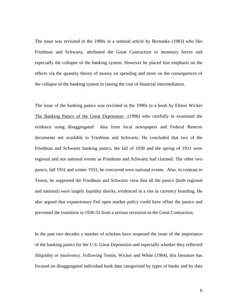
The issue was revisited in the 1980s in a seminal article by Bernanke (1983) who like

Friedman and Schwartz, attributed the Great Contraction to monetary forces and

especially the collapse of the banking system. However he placed less emphasis on the

effects via the quantity theory of money on spending and more on the consequences of

the collapse of the banking system in raising the cost of financial intermediation.

The issue of the banking panics was revisited in the 1990s in a book by Elmus Wicker

The Banking Panics of the Great Depression (1996) who carefully re examined the

evidence using disaggregated data from local newspapers and Federal Reserve

documents not available to Friedman and Schwartz. He concluded that two of the

Friedman and Schwartz banking panics, the fall of 1930 and the spring of 1931 were

regional and not national events as Friedman and Schwartz had claimed. The other two

panics, fall 1931 and winter 1933, he concurred were national events. Also, in contrast to

Temin, he supported the Friedman and Schwartz view that all the panics (both regional

and national) were largely liquidity shocks, evidenced in a rise in currency hoarding. He

also argued that expansionary Fed open market policy could have offset the panics and

prevented the transition in 1930-31 from a serious recession to the Great Contraction.

In the past two decades a number of scholars have reopened the issue of the importance

of the banking panics for the U.S. Great Depression and especially whether they reflected

illiquidity or insolvency. Following Temin, Wicker and White (1984), this literature has

focused on disaggregated individual bank data categorized by types of banks and by data

7

sources, in contrast to the macro approach taken by Friedman and Schwartz and

Bernanke. Section 2 discusses some of this literature. Section 3 briefly examines why the

U. S. had so many bank failures and was so prone to banking panics in its history. Section

4 provides some econometric evidence on the issue of illiquidity versus insolvency and

also discusses some of the methodological issues in using macro time series versus using

disaggregated data. Section 5 compares the financial crises of the 1930s in the U.S. to the

recent financial crisis 2007-2008. Section 6 concludes with some lessons for policy.

2. The Recent Debate over U.S. Banking Panics in the 1930s: Illiquidity

versus Insolvency.

In this section we survey recent literature on whether the clusters of bank failures that

occurred between 1930 and 1933 were really panics in the sense of illiquidity shocks.1

This has important implications for the causes of the Great Depression. If the clusters of

bank failures were really panics then it would support the original Friedman and

Schwartz explanation. If the clusters of bank failures primarily reflected insolvency then

other factors such as a decline in autonomous expenditures or negative productivity

shocks (Prescott1999) must explain the Great Contraction.

Friedman and Schwartz viewed the banking panics as largely the consequence of

illiquidity, especially in 1930-31. Their key evidence was a decline in the deposit

currency ratio which lowered the money multiplier, money supply and nominal spending.

They describe the panic in the fall of 1930 as leading to “a contagion of fear’ especially

1 Panics can arise because of exogenous illiquidity shocks in the context of the Diamond and Dybvig ( 1983)

random withdrawals model or in the context of asymmetric information induced runs and panics

( Calomiris and Gorton, 1991)

8

after the failure of the Bank of United States in New York City in December. They also

discussed the effects of the initial banking panic leading to contagion by banks dumping

their earning assets in a “fire sale” in order to build up their reserves. This in turn led to

the failure of otherwise solvent banks. Wicker (1996) disputes whether the 1930 panic

and the spring 1931 Friedman and Schwartz panics were national in scope but agrees

with them that all four banking panics were liquidity shocks.

By contrast both Temin(1976) and White (1984), the latter using disaggregated data on a

sample of national banks, argued that the original 1930 banking panic was not a liquidity

event but a solvency event occurring in banks in agricultural regions in the south and the

Midwest which had been weakened by the recession. These small unit banks came out of

the 1920s in a fragile state reflecting declining agricultural prices and oversupply after

World War I. As in Wicker (1980) they identify the locus of the crisis as the collapse on

November 7 1930 of the Caldwell investment bank holding company of Nashville,

Tennessee on November 7, 1930, a chain bank (in which one holding company had a

controlling interest in a chain of banks), and its correspondent network across a half

dozen states.

Calomiris and Mason (2003), following the approach taken in Calomiris and Mason

(1997) to analyze a local banking panic in Chicago in June 1932, use disaggregated data

on all of the individual member banks of the Federal Reserve System to directly address

the question whether the clusters of banking failures of 1930-33 reflected illiquidity or

insolvency. Based on a survival duration model on 8700 individual banks they relate the

9

timing of bank failures to various characteristics of the banks as well as to local, regional

and national shocks. They find that a list of fundamentals including; bank size, the

presence of branch banking, net worth relative to assets as a measure of leverage; reliance

on demand debt; market power; the value of the portfolio; loan quality; the share of

agriculture; as well as several macro variables, largely explains the timing of the bank

failures. When they add into the regression as regressors the Friedman and Schwartz

panic windows (or Wicker’s amendments to them) they turn out to be of minimal

significance. Thus they conclude that ,with the exception of the 1933 banking panic,

which as Wicker (1996) argued reflected a cumulative series of state bank suspensions in

January and February leading to the national banking holiday on March 6, that illiquidity

was inconsequential.

Richardson (2007) provides a new comprehensive data source on the reasons for bank

suspensions from the archives of the Federal Reserve Board of Governors including all

Fed member banks and nonmember banks (both state and local) from August 1929 to just

before the bank holiday in March 1933. He also distinguished between temporary and

permanent suspensions. Based on a questionnaire asked by bank examiners after each

bank suspension, Richardson put together a complete list of the causes of each suspension.

The categories include: depositor runs, declining asset prices, the failure of

correspondents, mergers, mismanagement and defalcations. Richardson then classified

each bank suspension into categories reflecting illiquidity, insolvency or both. With this

data he then constructed indices of illiquidity and insolvency. His data shows that 60% of

the suspensions during the period reflected insolvency, 40% illiquidity. Moreover he

10

shows that the ratio of illiquidity to insolvency spikes during the Friedman and Schwartz

(and also Wicker) panic windows (see Figure 2.1). This evidence in some respects

complements the Friedman and Schwartz, Wicker stories and those of Temin and White.

During the panics illiquidity rises relative to insolvency; between the panics insolvency

increases relative to illiquidity. Consistent with the Friedman and Schwartz stories, the

panics were driven by illiquidity shocks seen in increased hoarding, but after the panics,

in the face of deteriorating economic conditions, bank insolvencies continued to rise. This

is consistent with the evidence of Temin and White. The failures continued through the

contraction until the banking holiday of the week of March 6, 1933 (with the exception of

the spring of 1932 while the Fed was temporarily engaged in open market purchases).

Richardson (2006) backs up the illiquidity story with detailed evidence on the 1930

banking panic. As in Wicker (1980) the failure of Caldwell and Co. in November was the

signature event of this crisis. Richardson uses his new data base to identify the cascade of

failures through the correspondent bank networks based on the Caldwell banks. During

this period most small rural banks maintained deposits on reserve with larger city banks

that in turn would clear their checks through big city clearinghouses and/or the Federal

Reserve System. When Caldwell collapsed so did the correspondent network. Moreover

Richardson and Troost (2009) clearly show that when the tidal wave from Caldwell hit

the banks of the state of Mississippi in December that the banks in the southern half of

the state under the jurisdiction of the Federal Reserve Bank of Atlanta fared much better

(had a lower failure rate) than those in the northern half under the jurisdiction of the

11

Figure 2.1: Bank Failures and Suspensions

12

.1

.2

.3

.4

.5

.6

I II III IV I II III IV I II III IV I II III IV I II III IV

1929 1930 1931 1932 1933

Ratio of Bank Suspensions due to Liquidity over All Bank Suspensions

.0

.2

.4

.6

.8


1929 1930 1931 1932 1933

Ratio of Bank Suspensions due to Insolvancy over All Bank Suspensions

-.6

-.4

-.2

.0

.2

.4


1929 1930 1931 1932 1933

Difference between Liquidity Ratio and Insolvancy Ratio (L/T-I/T)

13

Federal Reserve Bank of St. Louis. The Atlanta Fed followed Bagehot’s Rule discounting

freely the securities of illiquid but solvent member banks. The St. Louis Fed followed the

real bills doctrine and was reluctant to open the discount window to its member banks in

trouble. This pattern holds up when the authors control for fundamentals using a

framework like that in Calomiris and Mason (2003).2

Finally, Christiano et al (2004) build a DSGE model of the Great Contraction

incorporating monetary and financial shocks. They find that the key propagation channels

explaining the slump were the decline in the deposit currency ratio, amplified by

Bernanke, Gertler and Gilchrist’s (1996) financial accelerator. The liquidity shock

reduced funding for firms, lowering investment and firm’s net worth. At the same time

the increased currency hoarding reduced consumption expenditure. Their simulations,

like those of McCallum (1990) and Bordo, Choudhri and Schwartz (1995) show that

expansionary open market purchases could have offset these shocks.

In sum, the debate over illiquidity versus insolvency in the failures of U.S. banks hinges

on the use of aggregate versus disaggregated data. Aggregate data tends to favor

illiquidity and the presence of and importance of banking panics in creating the Great

Contraction. Disaggregate data tends to focus on insolvency driven by the recession and

to downplay the role of the panics in creating the Great Contraction. However the recent

more comprehensive data unearthed by Richardson as well as the Christiano et al model

suggests that the original Friedman and Schwartz story may well prevail.

2 Carlson ( 2008) shows that during the panic banks that would otherwise have merged with stronger banks

rather than fail were prevented from doing so.

14

3. Why Did the U.S. have so many banking panics?

We have argued that the signature event in the U.S. Great Contraction was the series of

banking panics from 1930-33. But this was nothing new in U.S. financial history. From

the early nineteenth century until 1914, the U.S. had a banking panic every decade. There

is a voluminous literature on U.S. financial stability and the lessons that come from that

literature are that the high incidence of banking instability reflected two forces: unit

banking and the absence of an effective lender of last resort.

3.1 Unit Banking

Fear of the concentration of economic power largely explains why states generally

prohibited branch banking and why since the demise of the Second Bank of the United

States in 1836 until quite recently there was no interstate banking (White 1983). Unit

banks, because their portfolios were geographically constrained were highly subject to

local idiosyncratic shocks. Branching banks, especially those which extended across

regions can better diversify their portfolios and protect themselves against local/regional

shocks.

A comparison between the experience of the U.S. and Canadian banking systems makes

the case (Bordo, Redish and Rockoff 1996). The U.S. until the 1920s has had

predominantly unit banking and until very recently a prohibition on interstate banking.

Canada since the late nineteenth century has had nationwide branch banking. Canada

only adopted a central bank in 1934. The U.S. established the Fed in 1914. Canada had

15

no banking panics since Confederation in 1867, the U.S. had nine. However the Canadian

chartered banks were always highly regulated and operated very much like a cartel under

the guidance of the Canadian Bankers Association and the Department of Finance.

3.2 A Lender of Last Resort

Since the demise of the Second Bank of the United States until the establishment of the

Federal Reserve in 1914, the U.S. has not had anything like a central bank to act as a

lender of last resort as the Bank of England had evolved into during the nineteenth

century (Bordo, 2007). Clearinghouses, established first in New York City in 1857 and

other major cities later, on occasion acted as a lender of last resort by pooling the

resources of the members and issuing clearinghouse loan certificates as a substitute for

scarce high powered money reserves. However on several prominent occasions before

1914 the clearinghouses did not allay panics (Timberlake, 1992). Panics were often ended

in the National Banking era by the suspension of convertibility of deposits into currency.

Also the U.S. Treasury on a few occasions performed lender of last resort functions.

The Federal Reserve was established to serve (amongst other functions) as a lender of last

resort but as documented above, failed in its task between 1930 and 1933. Discount

window lending to member banks was at the prerogative of the individual Federal

Reserve banks and as discussed above, some Reserve banks did not follow through.

Moreover until the establishment of the National Credit Corporation in 1931 (which

became the Reconstruction Finance Corporation in 1932) there was no monetary

16

authority to provide assistance to non member banks (Wicker, 1996). Wicker effectively

argues that the panics pre 1914 always were centered in the New York money market and

then spread via the vagaries of the National banking system to the regions. The New

York Fed, according to him, learned the lesson of the panics of the national banking

system and did prevent panics from breaking out in New York City during the Great

Contraction. But as he argues, it did not develop the tools to deal with the regional

banking panics which erupted in 1930 and 1931.

3.3 Recent Evidence

There is considerable empirical evidence going back to the nineteenth century on the case

linking unit banking to failures and panics (White, 1983). Cross country regression

evidence in Grossman (1994) and Grossman (2010) finds that during the 1930s countries

which had unit banking had a greater incidence of banking instability than those which

did not. For the U.S., Wheelock (1995) finds, based on state and county level data that

states that allowed branching had lower bank failure rates than those which did not.

However Carlson (2004) (also Calomiris and Mason, 2003) find based on a panel of

individual banks that state branch banks in the U.S. were less likely to survive the

banking panics. The reason Carlson gives is that while state branch banks can diversify

against idiosyncratic local shocks better than can unit banks they were still exposed to the

systemic shocks of the 1930s. He argues that branch banks used the diversification

opportunities of branching to increase their returns but also followed more risky

strategies such as holding lower reserves.

17

Carlson and Michener (2009) show, based on data on Californian banks in the 1930s

(California was a state that allowed branch banking) that the entry of large branching

networks, by improving the competitive environment actually improved the survival

probabilities of unit banks. They explain the divergent results between studies based on

individual banks and those based on state and county level data by the argument that the

U.S. banking system would have been less fragile in the 1930s had states allowed more

branching not because branch banks would have been more diversified but because the

system would have had more efficient banks.

4. Econometric Evidence

In this section an structural vector autoregression (SVAR) is estimated using aggregate

data on bank failures/suspensions, unemployment, money supply and a quality spread

which is the difference between the yield on a Baa rated bond and a composite yield on

10 year maturity Treasury bills. The data we use on bank failures/suspensions includes a

series on total bank failures/suspensions found in Table 12 of the 1937 Federal Reserve

Bulletin and two new series on bank failures/suspensions due to illiquidity and

insolvency from Richardson (2007).

The aim of this exercise is to identify illiquidity shocks from insolvency shocks in an

attempt to answer the question of the underlying fundamental causes of the financial

crises identified by Friedman and Schwartz (1963). The use of aggregate data is useful

for this aim in that we are able to identify common trends (or factors) affecting the

18

aggregate economy. This approach is in contrast to the literature on explaining bank

failures during the Great Depression that uses disaggregated micro data on banks at the

local, state, and regional level. This literature is successful at explaining why different

locations were affected in different ways during the financial crises but is silent on the

underlying common factors (if any) that were driving the crises.

Probably the best known paper from this literature, Calomiris and Mason (2003), utilize a

panel data set of Federal Reserve banks and estimate a bank survival duration model for

the period of great bank stress during the early 1930’s. This excellent paper claims,

among other things, that the bank failures during this period were local and regional in

nature and that their covariates, such as individual measures of bank stress, do a good job

of explaining why banks failed during the first three financial crises identified by

Friedman and Schwartz (1963). They show this by adding in crisis dummies for the three

periods (Oct-1930 to Jan-1931, March-1931 to Aug-1931, and Sept-1931 to Dec-1931)

into their log-logistic survival model and show that these event dummies add little to the

predicted bank failures generated by their model. Because the log-logistic survival model

has a time varying underlying hazard function what this study shows is that the event

dummy does not explain more than the baseline hazard function underlying their

econometric model.

Using this methodology with disaggregated data is therefore silent on whether the local

and regional bank failures that were observed were driven by underlying common factors

19

that were national in scope.3 What this study does show however is that the regional/local

differences in bank failures that are orthogonal to the underlying baseline hazard can be

explained by bank fundamentals. What we do not know is whether the underlying

baseline hazard was also driven by bank fundamentals or by common aggregate (or

national) factors. In general, we know of no disaggregated study that does allow for a

factor structure in the covariates of the model so that the nature of the common factors

affecting bank failures in the 1930s, if any, is still an open question.

This paper aims to contribute to this debate using the new series on bank failures

constructed by Richardson (2007). In this study, as mentioned above, Richardson uses

reports from the Federal Reserve Board to assign bank failures to one of two categories:

failure or suspension due to insolvency and failure or suspension (of otherwise solvent

banks) due to illiquidity. Our hope is that we can identify, using a structural VAR, the

underlying fundamental aggregate illiquidity and insolvency shocks and determine

whether they have any explanatory power in explaining bank failures. We see this study

as complimentary to the disaggregated studies noted above.

Figure 4.1 depicts the data we have on total number of bank failures and suspensions

(hereafter referred to as BFS, from Table 12 of the 1937 Federal Reserve Bulletin) and

the two series sourced from Richardson (2007). The shaded regions in the figure show

the Friedman and Schwartz

3 In their regression Calomiris and Mason (2003) do include national variables but find that they are not

significant. However, this means that the national variables do not explain the differences in bank

suspensions orthogonal to their baseline hazard which most likely contains the national factors impacting

ON bank suspensions.

20

Figure 4.1: Bank Failures and Suspensions Data

(1963) financial crises windows. It is apparent from the figure that the illiquidity and

insolvency series behave quite differently especially during the first crisis of 1931.

Through the use of a structural VAR we aim to extract from these series a set of

orthogonal illiquidity shocks and insolvency shocks with the hope of determining their

relevance to explaining the underlying behavior of the total bank failure series.

The data that we use from Richardson (2007) are his broad measures of bank

failures/suspensions due to illiquidity and insolvency. Richardson (2007, p. 602—603)

0

1

2

3

4

5

6

7

I II III IV I II III IV I II III IV I II III IV I II

1929 1930 1931 1932 1933

log of fails/suspensions due to insolvency

log of fails/suspensions due to illiquidity

log of total fails/suspensions

21

describes in detail exactly which suspensions are determined to be due to illiquidity and

which are due to insolvency. Banks included in the illiquidity series include those that

were suspended temporarily, those that closed permanently because of heavy withdrawals

and those that closed because of the failure of correspondent banks. Also included in the

broad definition are banks that were suspended because their assets were considered to be

slow or they failed to get loans from correspondent banks or they ran out of reserves. The

broad definition of banks that were deemed to have failed or suspended because of

insolvency included banks with slow, worthless, or frozen assets, depreciation of assets

(real estate, stocks and bonds), inability to collect loans, and local depression.

These two series do not sum up to total bank failures/suspensions. Reasons for this

include double counting (some banks were counted multiple times if they were suspended

temporarily, reopened and then subsequently closed) and the exclusion or two additional

categories explaining bank failure/suspension. These two categories include poor

management and defalcations (fraud or other reasons).

4.2 SVAR Analysis

The structural vector autoregression (SVAR) analysis presented here is an attempt to

identify the major shocks that contributed to the bank failures during the 1930’s. We

utilize five variables in this analysis: the unemployment rate, a measure of the quality

spread between commercial paper and treasury bonds, the logarithm of the money supply,

22

the logarithm of the number of bank failures due to illiquidity and the logarithm of the

total number of bank failures.

The SVAR takes the form of the AB-model from Amisano and Giannini (1997).

That is

t t

t t

A A L y A

A Bu (1)

where A(L) is a lag polynomial given by

5 1

p

pA L I A L A L (2)

and where jA is a 5 5 matrix for 1,...,j p . The structural shock

tu is a 5 1 vector of

shocks that has mean 0 and variance equal to 5I . The reduced for shocks,

t, are related

to the structural shocks in that

1

t tA Bu . (3)

23

Table 1: Results from ADF-GLS Unit Root Tests

Variable Deterministic Terms Lag Test Stat. Outcome

Unemployment Rate Constant 1 0.449 Do not reject H0

Quality Spread Constant 0 -1.113 Do not reject H0

Log Money Supply Constant, trend 0 -1.410 Do not reject H0

Log Bank Failures due to

Liquidity

Constant 0 -2.974*** Reject H0

Log Total Bank Failures Constant 0 -2.890*** Reject H0

*** Significant at 1% level. The null hypothesis, H0, is that the time series contains a unit root.

The matrix A represents the contemporaneous relationships amongst the endogenous

variables of the system while the matrix B represents the contemporaneous relationships

between the structural shocks and the reduced form shocks. In our identification we

assume that B is a diagonal matrix whose elements are the standard deviations of the

structural shocks. Our identification therefore rests on imposing at least 10 restrictions on

the elements of A.

Before outlining the identification strategy we first discuss the nature of the time

series that makes up our model. Table 1 reports the results of the Elliot, Rothenberg, and

Stock (1996) unit root test. For each variable the null hypothesis is that the time series

contains a unit root and for each variable the lag length is chosen using the modified

Schwarz Information Criterion.

The results are that for the unemployment rate, the quality spread, and the log of

money supply, there is not enough evidence to reject the null that each series contains a

unit root. Hence each of these series will enter the SVAR in first differences. For the log

24

of bank failures due to illiquidity and the log of total bank failures there is enough

evidence at the 1% level to reject the null that each series contains a unit root in favor of

the alternative that each series is stationary. Hence, both the bank failure series will enter

the SVAR in log-levels.

As noted above, in order for us to estimate our SVAR we need to impose

restrictions on the matrices A and B. The first sets of restrictions are that B is a diagonal

matrix. This, however is not enough to identify the system so we need to impose

restrictions on A. The exact form of the structural model given in (3) is

1 11 1t tb u (4a)

2 21 1 25 5 22 2t t t ta a b u (4b)

3 32 2 33 3t t ta b u (4c)

4 44 4t tb u (4d)

5 53 3 54 4 55 5t t t ta a b u . (4e)

Equation (4a) identifies the first structural shock as the innovation to

unemployment. The identification assumption used here is that none of the other

variables in the system contemporaneously impact unemployment; the other variables

only impact unemployment with a lag. While this is an identifying assumption, tests

outlined below do not find any evidence to suggest that any of the other variables do in

fact affect unemployment contemporaneously. Equation (4b) identifies the innovation to

the quality spread by assuming that it is contemporaneously affected by unemployment

and the total number of bank failures. We assume that money supply and bank failures

due to illiquidity do not contemporaneously impact the quality spread and statistical tests

25

suggest that this hypothesis cannot be rejected at any reasonable level of significance. 4

Thus the second structural shock is a shock to the quality spread and is designed to

capture the disintermediation effects of bank failures noted in Bernanke (1982). The third

equation, (4c), deals with the impact that the crises had on money supply. Our

assumption is that innovations to the quality spread impacts the money supply but that the

other three variables do not. We are explicitly assuming that innovations to

unemployment and bank failures do not contemporaneously affect the money supply.

From our tests these assumptions cannot be rejected but it is clear that it is difficult to

give a clear interpretation to the third structural shock, 3tu . It is most likely an amalgam

of money demand and supply shocks but we are unable to disentangle these in our

identification.

The fourth equation is the equation for bank failures for illiquidity reasons. As

noted in Richardson (2007) this data is collected from reports to the Federal Reserve

Board by bank examiners at the time the bank failed. The bank examiners examined the

bank’s accounts and based on their reading of the books, determined the reason for the

bank’s failure. Richardson (2007) used these reports to divide the reported bank failures

into categories including failures due to insolvency and failures due to illiquidity. In

equation (4d) we identify the structural illiquidity shock as the innovation to this series.

We take the stand that the bank examiners had no reason to classify insolvent banks as

illiquid and so assume that the examiners, who had access to the bank’s account at the

time of their failure, were correct in their designation of cause of failure.

4 When we include the innovation to bank failures due to illiquidity we find the coefficient on this

innovation and the innovation to total bank failures are both insignificant. This is probably due to near

multicollinearity and so we drop the innovation to bank failures due to illiquidity from the identifying

equation 4(b).

26

The last equation (4e) aims to identify the orthogonal component of the illiquidity

bank shock in total bank failures. This orthogonal shock includes all other reasons for a

bank’s failure, most notable insolvency. The identifying assumption is that the failure of

insolvent banks would not immediately affect illiquid but otherwise solvent banks, at

least in the short run. However, the solvency shock may also cause, through contagion, a

run on otherwise healthy banks, especially if there was a run up of closures of insolvent

banks preceding the bank run. Our identifying assumption is that if the insolvency shock

causes a bank run then this will happen with a time lag. That is, the identifying

assumption is that while the illiquidity shock might cause some insolvent banks to fail

contemporaneously the insolvency shock will lead to failures due to illiquidity only with

a lag.

Thus we identify five shocks in total that we interpret as follows: a shock to the

real side of the economy via unemployment, a shock to the quality spread – a

disintermediation shock, a shock to the money supply, the illiquidity shock causing banks

to fail and a shock causing banks to fail that is orthogonal to the illiquidity shock – most

likely caused by insolvencies.

The SVAR described in (1) – (4) is estimated with p chosen to be 1 by

minimizing Akaike’s Information Criterion. The scoring algorithm of Amisano and

Giannini (1997) is used to estimate the parameters in (4). The estimates for A and B are

reported in Table 2 while the estimates for A1, the lag matrix, are reported in Table 3.

The sample period used (based on Richardson’s data) finished in February, 1933 and so

does not include the period of the bank holiday starting on March 6, 1933.

27

Table 2 reports the estimates for the non-zero elements of A and B. All but the coefficient

on the innovation to money supply in equation (4e) are significant at the 5% level. Table

2 also reports the test of over-identifying restrictions which is a test that all of the

restrictions imposed on A and B are valid versus there is at least one restriction that is not

valid. This test has a p-value of 0.823 which implies that there is no statistical evidence to

suggest that the restrictions placed on A and B are not valid.

A full discussion of all the impulse response functions can be found in the

appendix. In what follows we summarize our findings and highlight the important

conclusions. Figure 1 shows the impulse response functions for total bank

failures/suspensions and Table 4 reports the forecast error variance decomposition. It is

clear from Figure 1 that the illiquidity shock has a large and persistent effect on total

bank failures/suspensions. The other two shocks that also appear to have a significant

impact on bank failures are the unemployment shock and the bank failure shock that is

orthogonal to the illiquidity shock. The unemployment shock’s impact hits is maximum

three months after the initial shock while the non-liquidity bank failure shock reaches its

maximum impact two months after the initial shock. A shock to the spread between BAA

securities and a 10 year treasury bond has a positive, albeit insignificant, impact on bank

failures while a positive money shock has a negative impact on bank failures. This

negative impact reinforces the views of Christiano et al (2004), McCallum (1990) and

Bordo, Choudhri and Schwartz (1995).

28

Table 2: Structural Estimates

Coefficient Estimate Std. Error t-Statistic P-value

21a 0.263 0.115 2.296 0.022

32a -0.006 0.004 -1.657 0.098

53a -2.922 2.555 -1.144 0.253

54a 0.630 0.065 9.565 0.000

25a 0.388 0.190 2.047 0.041

11b 0.741 0.079 9.381 0.000

22b 0.563 0.060 9.376 0.000

33b 0.015 0.002 9.374 0.000

44b 0.584 0.062 9.381 0.000

55b 0.255 0.027 9.366 0.000

Log likelihood -4.720

LR test for over-identification:

Chi-square(5) 2.183 Probability 0.823

Table 3: Reduced Form Estimates of (1)

U Q m _bf l _bf t

( 1)U 0.374** 0.022 -0.002 0.237* 0.264***

(0.156) (0.133) (0.003) (0.122) (0.097)

( 1)Q -0.069 0.083 -0.003 0.062 0.097

(0.199) (0.170) (0.004) (0.157) (0.124)

( 1)m -13.578* -0.498 -0.439** -1.138 0.545

(8.061) (6.869) (0.167) (6.351) (4.998)

_ ( 1)bf l 0.187 0.072 -0.001 -0.584** -0.295*

(0.299) (0.255) (0.006) (0.236) (0.186)

_ ( 1)bf t -0.552 -0.312 -0.011 1.650*** 1.007***

(0.421) (0.359) (0.009) (0.332) (0.262)

Constant 2.124* 1.238 0.047** -2.196*** 0.873

(1.094) (0.932) (0.022) (0.862) (0.679)

R-squared 0.197 0.064 0.267 0.636 0.596

Adj. R-squared 0.092 -0.058 0.171 0.588 0.543

Sum sq. resids 20.86515 15.14943 0.008954 12.95158 8.020456

S.E. equation 0.741001 0.631403 0.015350 0.583807 0.459418

* significant at 10% level, ** sig. at 5% level, *** sig. at 1% level.

U : unemployment rate, Q: spread between BAA paper and composite 10 year Treasury Bill

m: log of money supply, bf_l: log of bank failures due to illiquidity, bf_t: log of total bank failures.

29

Figure 1: Impulse Response of Total Bank Failures to Structural Shocks

-.4

-.2

.0

.2

.4

.6

1 2 3 4 5 6 7 8 9 10

Response to Unemployment Shock

-.4

-.2

.0

.2

.4

.6

1 2 3 4 5 6 7 8 9 10

Response to Quality Spread Shock

-.4

-.2

.0

.2

.4

.6

1 2 3 4 5 6 7 8 9 10

Response to Money Shock

-.4

-.2

.0

.2

.4

.6

1 2 3 4 5 6 7 8 9 10

Response to Liquidity Shock

-.4

-.2

.0

.2

.4

.6

1 2 3 4 5 6 7 8 9 10

Response to Other Bank Failure Shock

30

The forecast error variance decompositions show that the liquidity shock accounts

for roughly 40% of the forecast error with the other bank failure shock (which includes

failures due to insolvencies) shock only accounting for 30% of the forecast error variance

in the long run. The other shock that plays an important role is the unemployment (or real

side) shock which also accounts for approximately 30% of the forecast error variance of

total bank failures in the long run. Thus it appears that the illiquidity shock is very

important for explaining total bank failures/suspensions.

Table 4: Variance Decomposition of Total Bank Failures

Period Unemployment

Shock Disintermediation

Shock Money

Shock Illiquidity

Shock Other Bank Failure

Shock

1 0.01 0.05 0.92 66.94 32.09

2 12.60 1.09 0.88 48.82 36.62

3 22.66 1.48 1.52 42.24 32.10

4 26.07 1.50 1.78 40.19 30.46

5 26.90 1.50 1.86 39.68 30.05

6 27.06 1.49 1.88 39.59 29.98

7 27.08 1.49 1.88 39.57 29.97

8 27.08 1.49 1.88 39.57 29.97

9 27.08 1.49 1.88 39.57 29.97

10 27.08 1.49 1.88 39.57 29.97

The impulse response functions together with the variance decompositions show that the

liquidity shock is very important in explaining the bank failures/suspensions during the

early 1930’s.

31

In order to determine if the liquidity shocks played a role during the particular

financial crisis windows identified by Friedman and Schwartz (1963) we now turn to

historical decompositions. Figure 2 contains historical decompositions for the total bank

failures/suspensions series. Each panel of Figure 2 contains a simulated total bank

failures/suspensions series under the hypothesis that only one structural shock was

driving the stochastic component of the data. Thus the series titled liquidity shock shows

the generated series if there was only a liquidity shock.

Figure 2: Historical Decompositions of Total Bank Failures/Suspensions

0

100

200

300

400

500

600

III IV I II III IV I II III IV I II III IV I

1929 1930 1931 1932 1933

Total Number of Bank Suspensions

Historical Decomposition - Liquidity Shock

Historical Decomposition - Other Bank Failure Shock

Historical Decomposition - Unemployment Shock

32

The results of the historical decompositions clearly point to the liquidity shock playing a

significant role in the bank failures during the Friedman and Schwartz crisis windows.

The most obvious case is during the second window from March, 1931 to August, 1931.

Here the historical decomposition for the liquidity series almost completely mimics the

actual data. The other shocks do not spike in this window at all.

For the first crisis window both the series generated using only liquidity shocks

and the series generated using the orthogonal component to the liquidity shock both peak

at the same time. The series generated with the unemployment shock also peaks. It is

clear that in this crisis window all three major shocks play a role. For the third window

from September 1931 until December 1931 the orthogonal bank failure shock plays the

most important role, at least for the first peak in this window. For the second spike in

bank failures during this window it appears the liquidity shock and the unemployment

shock better mimic the data. At the end of the sample at the end of 1932 and heading into

the last crisis window the liquidity shock best explains the sharp increase in bank failures.

To summarize we have estimated a structural VAR in order to identify a set of

shocks including liquidity shocks for the 1930’s. The impulse response functions

obtained from this structural VAR make sense and show that the liquidity shock is an

important shock for explaining the observed bank failures/suspensions series. Further, the

historical decompositions show that the liquidity shock played an important role in all but

one of the peaks to the bank failure series; the peak in January of 1932.

Finally, we should caution that the results obtained above are obtained from a

small structural VAR and so do not have a full structural interpretation. For example we

have not included wages or prices and we have not identified money supply and money

33

demand shocks separately from each other, nor have we identified aggregate demand and

supply shocks separately from each other. We have only identified shocks to money

supply and to unemployment but cannot say whether these are due to demand or supply

shocks.

5. A Comparison of the Financial Crisis in the U.S. to the 2007-2008 Crisis

Many people have invoked the experience during the Great Contraction and especially

the banking crises of 1929-33 as a good comparison to the financial crisis and Great

Recession of 2007-2009. In several descriptive figures in this section we compare the

behavior of some key variables between the two events. We demarcate the crisis

windows in the Great Contraction using Friedman and Schwartz’s dates. For the recent

period we use Gorton’s (2010) characterization of the crisis as starting in the shadow

bank repo market in August 2007 (dark grey shading)and then changing to a panic in the

Universal banks after Lehman failed in September 2007 (light grey shading) . In most

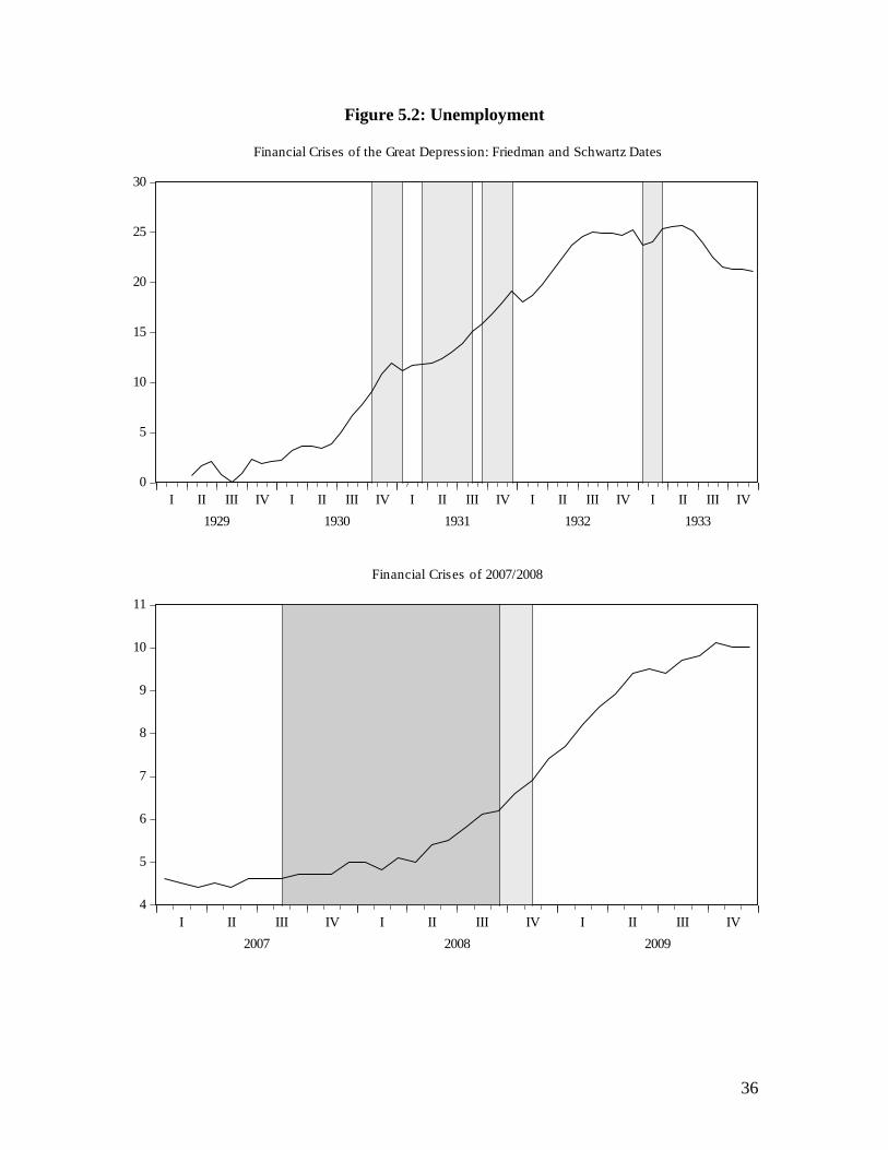
respects, e.g. the magnitude of the decline in real GDP and the rise in unemployment (see

Figures 5.1 and 5.2) the two events are very different but there are some parallels in

recent events to the 1930s. In Figure 5.1 we report real GNP for the 1930’s and the

2007—2009 normalized to be 100 at the start of each period. It is quite clear that the

contraction in late 2007 was mild (only about 5% peak to trough) relative to Great

Contraction in the 1930’s (roughly 35% peak to trough). The same is clear for

unemployment which is depicted in Figure 5.2. Unemployment rose from near 0% at the

start of the Great Contraction to slightly over 25% by the end of the contraction whereas

34

the rise in unemployment from 4% to 10% for the most recent contraction is small in

comparison.

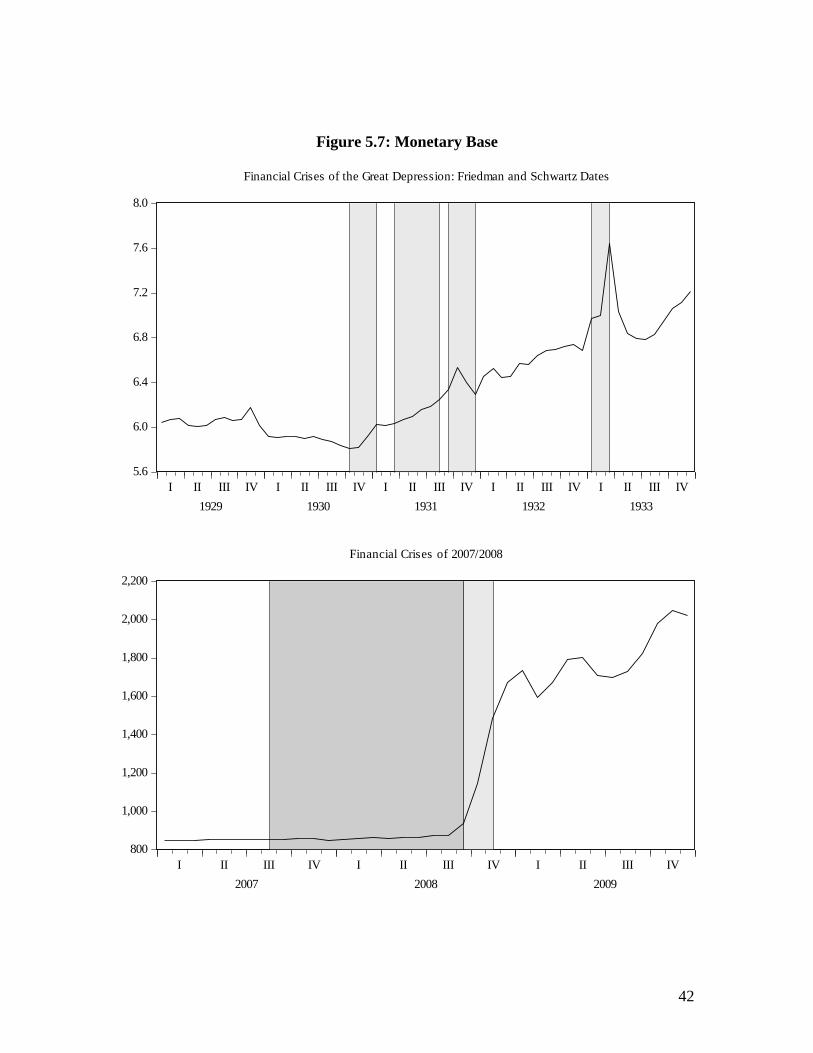
As discussed above the signature of the Great Contraction was a collapse in the money

supply brought about by a collapse in the public’s deposit currency ratio, a decline in the

banks deposit reserve ratio and a drop in the money multiplier (see Figures 5.3-5.6). In

the recent crisis M2 did not collapse, indeed it rose reflecting expansionary monetary

policy. Moreover the deposit currency ratio did not collapse in the recent crisis, it rose.

There were no runs on the commercial banks because depositors knew that their deposits

were protected by federal deposit insurance which was introduced in 1934 in reaction to

the bank runs of the 1930s. The deposit reserve ratio declined reflecting an expansionary

monetary policy induced increase in banks excess reserves rather than a scramble for

liquidity as in the 1930s. The money multiplier declined in the recent crisis largely

explained by a massive expansion in the monetary base reflecting the Fed’s doubling of

35

Figure 5.1: Real GNP (quarterly data)

60

70

80

90

100

110


1929 1930 1931 1932 1933

Financial Crises of the Great Depression: Friedman and Schwartz Dates

98

99

100

101

102

103

104

I II III IV I II III IV I II III IV

2007 2008 2009

Financial Crises of 2007/2008

36

Figure 5.2: Unemployment

0

5

10

15

20

25

30


1929 1930 1931 1932 1933


4

5

6

7

8

9

10

11


2007 2008 2009


37

its balance sheet in 2008 (see Figure 5.7). Moreover although a few banks failed recently,

they were miniscule relative to the 1930s (Figure 5.8) as were deposits in failed banks

relative to total deposits (see Figure 5.9).5

Thus the recent financial crisis and recession was not a pure Friedman and Schwartz

money story. It was not driven by an old fashioned contagious banking panic. But like

1930-33 there was a financial crisis. It reflected a run in August 2007 on the Shadow

Banking system which was not regulated by the central bank nor covered by the financial

safety net. According to Eichengreen (2008) its rapid growth was a consequence of the

repeal in 1999 of the Depression era Glass Steagall Act of 1935 which had separated

commercial from investment banking. These institutions held much lower capital ratios

than the traditional commercial banks and hence were considerably more prone to risk.

When the crisis hit they were forced to engage in major deleveraging involving a fire sale

of assets into a falling market which in turn lowered the value of their assets and those of

other financial institutions. A similar negative feedback loop occurred during the Great

Contraction according to Friedman and Schwartz.

According to Gorton (2010) the crisis centered in the repo market (sale and repurchase

agreements) which had been collateralized by opaque (subprime) mortgage backed

securities by which investment banks and some universal banks had been funded. The

5 The large spike in 1933 in both figures 5.7 and 5.8 largely represents the Bank holiday of March 6-10 in

which the entire nation’s banks were closed and an army of examiners determined whether they were

solvent or not. At the end of the week one sixth of the nation’s banks were closed. The relatively large

spike in 2008 in the deposits in failed bank series reflected the failure and reorganization by the FDIC of

Countrywide bank. Compared to the case in the 1930s failures there were no insured depositor losses.

38

Figure 5.3: Money Stock (M2)

28

32

36

40

44

48

52


1929 1930 1931 1932 1933


7,000

7,200

7,400

7,600

7,800

8,000

8,200

8,400

8,600


2007 2008 2009


39

Figure 5.4: Ratio of Deposits to Currency in Circulation

4

5

6

7

8

9

10

11

12


1929 1930 1931 1932 1933


4.9

5.0

5.1

5.2

5.3

5.4

5.5

5.6

5.7

5.8


2007 2008 2009


40

Figure 5.5: Ratio of Deposits to Reserves

7

8

9

10

11

12

13

14


1929 1930 1931 1932 1933


2.5

3.0

3.5

4.0

4.5

5.0

5.5


2007 2008 2009


41

Figure 5.6: Ratio of M2 to Monetary Base

3

4

5

6

7

8


1929 1930 1931 1932 1933


4

5

6

7

8

9

10


2007 2008 2009


42

Figure 5.7: Monetary Base

5.6

6.0

6.4

6.8

7.2

7.6

8.0


1929 1930 1931 1932 1933


800

1,000

1,200

1,400

1,600

1,800

2,000

2,200


2007 2008 2009


43

Figure 5.8: Numbers of Failed Banks

0

500

1,000

1,500

2,000

2,500

3,000

3,500


1929 1930 1931 1932 1933


0

5

10

15

20

25


2007 2008 2009


44

Figure 5.9: Deposits in Failed Banks as a proportion of Total Deposits

.00

.02

.04

.06

.08

.10

.12

.14


1929 1930 1931 1932 1933


.00

.01

.02

.03

.04

.05


2007 2008 2009


45

repo crisis continued through 2008 and then morphed into an investment/universal bank

crisis after the failure of Lehman Brothers in September 2008. The crisis led to a credit

crunch which led to a serious, but compared to the Great Contraction, not that serious

recession (see figures 5.1 and 5.2). The recession was attenuated in 2009 by expansionary

monetary and fiscal policy.

Figure 5.10 compares the Baa- Ten year Composite Treasury spread between the two

historical episodes. This spread is often used as a measure of credit market turmoil

(Bordo and Haubrich 2010). As can be seen the spike in the spread in 2008 is not very

different from that observed in the early 1930s.

5.1 The Recent Crisis in more detail.

The crisis occurred following two years of rising policy rates. Its causes include: major

changes in regulation, lax regulatory oversight, a relaxation of normal standards of

prudent lending and a period of abnormally low interest rates. The default on a significant

fraction of subprime mortgages produced spillover effects around the world via the

securitized mortgage derivatives into which these mortgages were bundled, to the balance

sheets of investment banks, hedge funds and conduits( which are bank owned but off

their balance sheets) which intermediate between mortgage and other asset backed

commercial paper and long-term securities. The uncertainty about the value of the

securities collateralized by these mortgages spread uncertainty through the financial

system about the soundness of loans for leveraged buyouts. All of this led to the freezing

46

Figure 5.10: Quality Spread (Baa – 10 year T-Bill)

1

2

3

4

5

6

7

8


1929 1930 1931 1932 1933

Financial Crises for the Great Depression: Friedman and Schwartz

1

2

3

4

5

6


2007 2008 2009

Financial Crises for 2007/2008

47

of the interbank lending market in August 2007 and substantial liquidity injections by the

Fed and other central banks.

The Fed then both extended and expanded its discount window facilities and cut the

federal funds rate by 300 basis points. The crisis worsened in March 2008 with the rescue

of the Investment bank, Bear Stearns, by JP Morgan backstopped by funds from the

Federal Reserve. The rescue was justified on the grounds that Bear Stearns exposure to

counterparties was so extensive that a worse crisis would follow if it were not bailed out.

The March crisis also led to the creation of a number of new discount window facilities

whereby investment banks could access the window and which broadened the collateral

acceptable for discounting. The next major event was a Federal Reserve Treasury bailout

and partial nationalization of the insolvent GSEs, Fannie and Freddie Mac in July 2008

on the grounds that they were crucial to the functioning of the mortgage market.

Events took a turn for the worse in September 2008 when the Treasury and Fed allowed

the investment bank Lehman Brothers to fail to discourage the belief that all insolvent

institutions would be saved in an attempt to prevent moral hazard. It was argued that

Lehman was both in worse shape and less exposed to counterparty risk than Bear Stearns.

The next day the authorities bailed out and nationalized the insurance giant AIG fearing

the systemic consequences for collateralized default swaps (insurance contracts on

securities) if it were allowed to fail. The fallout from the Lehman bankruptcy then turned

the liquidity crisis into a full fledged global credit crunch and stock market crash as

interbank lending effectively seized up on the fear that no banks were safe.

48

In the ensuing atmosphere of panic, along with Fed liquidity assistance to the commercial

paper market and the extension of the safety net to money market mutual funds, the US

Treasury sponsored its Troubled Asset Relief Plan (TARP) whereby $ 700 billion could

be devoted to the purchase of heavily discounted mortgage backed and other securities to

remove them from the banks’ balance sheets and restore bank lending. As it later turned

out most of the funds were used to recapitalize the banks.

In early October the crisis spread to Europe and to the emerging market countries as the

global interbank market ceased functioning. The UK authorities responded by pumping

equity into British banks, guaranteeing all interbank deposits and providing massive

liquidity. The EU countries responded in kind. And on October 13 2008 the US Treasury

followed suit with a plan to inject $250 into the U.S. banks, to provide insurance of

senior interbank debt and unlimited deposit insurance for non interest bearing deposits.

These actions ended the crisis. Expansionary Federal Reserve policy at the end of 2008,

lowering the funds rate close to zero, followed by a policy of quantitative easing: the

open market purchases of long-term Treasuries and mortgage backed securities finally

attenuated the recession by the summer of 2009.

Unlike the liquidity panics of the Great Contraction the deepest problem facing the

financial system was insolvency. This was only recognized by the Fed after the

September 2008 crisis. The problem stemmed from the difficulty of pricing securities

backed by a pool of assets, whether mortgage loans, student loans, commercial paper

49

issues, or credit card receivables. Pricing securities based on a pool of assets is difficult

because the quality of individual components of the pool varies and unless each

component is individually examined and evaluated, no accurate price of the security can

be determined.

As a result, the credit market, confronted by financial firms whose portfolios were filled

with securities of uncertain value, derivatives that were so complex the art of pricing

them had not been mastered, was plagued by the inability to determine which firms were

solvent and which were not. Lenders were unwilling to extend loans when they couldn’t

be sure that a borrower was creditworthy. This was a serious shortcoming of the

securitization process that was responsible for the paralysis of the credit market.

Finally another hallmark of the recent crisis which was not present in the Great

Contraction is that the Fed and other US monetary authorities engaged in a series of

bailouts of incipient and actual insolvent firms deemed too systemically connected to fail.

These included Bear Stearns in March 2008, the GSEs in July and AIG in September.

Lehman Brothers had been allowed to fail in September on the grounds that it was both

insolvent and not as systemically important as the others and as was stated well after the

event that the Fed didn’t have the legal authority to bail it out. The extension of the “Too

Big To Fail” doctrine which had begun in 1984 with the bailout of Continental Illinois

bank may be the source of future crises.

50

6. Conclusion: Some policy lessons from history.

In this paper we have reexamined the issue of the role of the banking panics between

1930 and 1933 in creating the Great Contraction. We focused on the debate between

those following the Friedman and Schwartz view that the banking crises were illiquidity

shocks and those following the Temin approach who view the clusters of banking

failures as not being liquidity driven panics but insolvencies caused by the recession.

Our survey of the evidence suggests that the banking crises did reflect contagious

illiquidity. But also that endogenous insolvency was important between the panics. Bank

failures regardless of their genesis contributed to the depression by reducing the money

supply and by crippling the credit mechanism.

Our empirical results showed that illiquidity played a major role in the financial crises of

late 1930 and all 1931. We estimated a VAR and used a triangular ordering to identify a

set of shocks including illiquidity and insolvency shocks. The impulse response functions

obtained from this orthogonalized VAR make sense and show that the illiquidity shock is

an important shock for explaining the observed bank failures/suspensions series. Further,

the historical decompositions show that the financial crisis of late 1930 and all of 1931

are well modeled as illiquidity crises. The financial crisis of 1933 is better explained as

an insolvency crisis.

The Federal Reserve learned the Friedman and Schwartz lesson from the banking panics

of the 1930s of the importance of conducting expansionary open market policy to meet

51

all of the demands for liquidity (Bernanke 2002). In the recent crisis the Fed conducted

highly expansionary monetary policy in the fall of 2007 and from late 2008 to the present.

Also , based on Bernanke’s 1983 view that the banking collapse led to a failure of the

credit allocation mechanism, the Fed, in conjunction with the Treasury, developed a

plethora of extensions to its discount window referred to as credit policy (Goodfriend,

2009) to encompass virtually every kind of collateral in an attempt to unclog the blocked

credit markets.

Some argue that for the first three quarters of 2008 that Fed monetary policy was actually

too tight seen in a flattening of money growth and the monetary base and high real

interest rates (Hetzel, 2009). Although the Fed’s balance sheet surged, the effects on high

powered money were sterilized. This may have reflected concern that rising commodity

prices at the time would spark inflationary expectations. By the end of the third quarter of

2008 the sterilization ceased evident in a doubling of the base.

The Fed’s credit policy involved providing credit directly to markets and firms the Fed

deemed most in need of liquidity and exposed the Fed to the temptation to politicize its

selection of the recipients of its credit (Schwartz 2009). In addition the Fed’s balance

sheet ballooned in 2008 and 2009 with the collateral of risky assets including those of

non banks. These assets were in part backed by the Treasury. The Fed also worked

closely with the Treasury in the fall of 2008 to stabilize the major banks with capital

purchases and stress testing. Moreover the purchase of mortgage backed securities in

2009 (quantitative easing) combined monetary with fiscal policy. These actions which

52

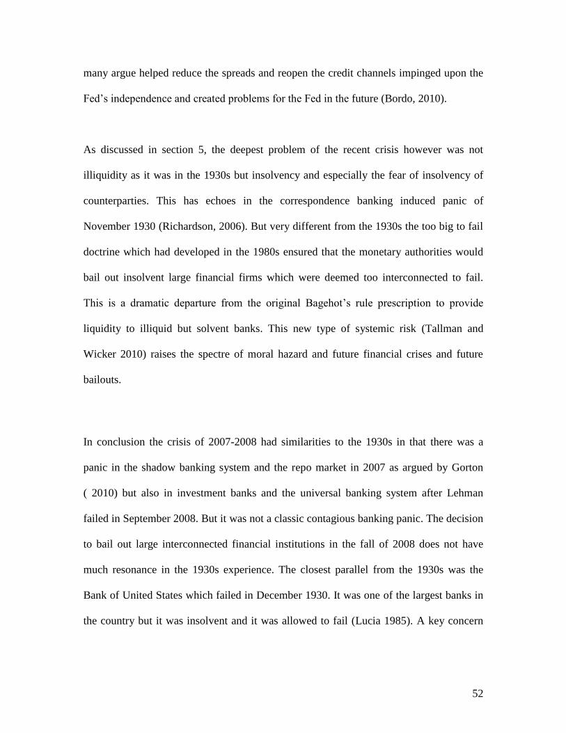
many argue helped reduce the spreads and reopen the credit channels impinged upon the

Fed’s independence and created problems for the Fed in the future (Bordo, 2010).

As discussed in section 5, the deepest problem of the recent crisis however was not

illiquidity as it was in the 1930s but insolvency and especially the fear of insolvency of

counterparties. This has echoes in the correspondence banking induced panic of

November 1930 (Richardson, 2006). But very different from the 1930s the too big to fail

doctrine which had developed in the 1980s ensured that the monetary authorities would

bail out insolvent large financial firms which were deemed too interconnected to fail.

This is a dramatic departure from the original Bagehot’s rule prescription to provide

liquidity to illiquid but solvent banks. This new type of systemic risk (Tallman and

Wicker 2010) raises the spectre of moral hazard and future financial crises and future

bailouts.

In conclusion the crisis of 2007-2008 had similarities to the 1930s in that there was a

panic in the shadow banking system and the repo market in 2007 as argued by Gorton

( 2010) but also in investment banks and the universal banking system after Lehman

failed in September 2008. But it was not a classic contagious banking panic. The decision

to bail out large interconnected financial institutions in the fall of 2008 does not have

much resonance in the 1930s experience. The closest parallel from the 1930s was the

Bank of United States which failed in December 1930. It was one of the largest banks in

the country but it was insolvent and it was allowed to fail (Lucia 1985). A key concern

53

from the bailouts of 2008 is that in the future the too big to fail doctrine will lead to

excessive risk taking by such firms and future crises and bailouts.

References

Gianni Amisano and Carlo Giannini (1997). Topics in Structural VAR Econometrics (2nd

Edition). Berlin. Springer-Verlag.

Ben Bernanke (1983) “Non Monetary Effects of the Financial Crisis in the Propagation

of the Great Depression” American Economic Review vol 73 ,pp 257-276

Ben Bernanke (2002) ‘On Milton’s Ninetieth Birthday’ speech given at the University of

Chicago November 8 2002.

Ben Bernanke, Simon Gilchrist and Mark Gertler (1996) “The Financial Accelerator and

the Flight to Quality” Review of Economics and Statistics, Vol 78. No.1 Feb pp 1-

15.

Michael D. Bordo,( 1986) “Explorations in Monetary History” Explorations in Economic

History Vol 23 pp339-415.

Michael D.Bordo , Ehsan Choudhri and Anna J Schwartz (1995) ‘Could Stable Money

Have Averted the Great Contraction” Economic Inquiry. Vol 33, pp 484-505.

Michael D. Bordo, Angela Redish and Hugh Rockoff (1996) “The U.S. Banking System

from a Northern Exposure: Stability versus Efficiency” Journal of Economic

History. Vol 54. No.2 June pp 325-341.

Michael D. Bordo (2007) “The History of Monetary Policy”, New Palgrave Dictionary of

Economics. Second Edition. New York MacMilllan

54

Michael D. Bordo (2010) “The Federal Reserve: Independence Gained, Independence

Lost…’ Shadow Open Market Committee March 26.

Michael D. Bordo and Joseph Haubrich (2010) “ Credit Crises, Money and Contractions:

An Historical View.’ Journal of Monetary Economics. Vol 57. No.1 January pp 1-

18.

Charles Calomiris and Joseph Mason (1997) “Contagion and Bank Failures During the

Great Depression: The June 1932 Chicago Banking Panic.” American Economic

Review. Vol 87(5). Pp 863-883.

Charles Calomiris and Joseph Mason (2003) “ Fundamentals, Panics and Bank Distress

During the Depression” American Economic Review Vol 93(5) , pp 1615-1647.

Chales Calomiris and Gary Gorton (1991) “The Origins of Banking Panics: Models,

Facts and Bank Regulation’ in R. Glenn Hubbard. Financial markets and

Financial Crises. Chicago: University of Chicago Press. Pp 109-173

Mark Carlson (2004) “ Are Branch Banks Better Survivors? Evidence from the

Depression Era” Economic Inquiry Vol 42(1) pp 111-126

Mark Carlson and Kris J. Mitchener (2006) “ Branch Banking, Bank Competition and

Financial Stability” Journal of Money, Credit and Banking” Vol 38. No.5 August

pp 1293-1326.

Mark Carlson (2008) “Alternatives for Distressed Banks and the Panics of the Great

Depression” Finance and Economic Discussion Series. Federal Reserve Board.

Washington DC

55

Mark Carlson and Kris J Mitchener (2009). “Branch Banking as a Device for Discipline:

Competition and Bank survivorship During the Great Depression” Journal of

Political Economy, Vol 117. No.2 pp 165-210.

Lawrence Christiano, Roberto Motto and Massimo Rostagno (2003). “The Great

Depression and the Friedman and Schwartz Hypothesis” Journal of Money,

Credit and Banking. Vol 35, pp 1119-1198.

Douglas Diamond and Phillip Dybvig (1983) “Bank Runs, Deposit Insurance, and

Liquidity,” Journal of Political Economy, Vol 91, No 3, pp 401—419.

Barry Eichengreen (2008) “Origins and Responses to the Crisis” UC Berkeley ( mimeo)

October.

Graham Elliot, Thomas Rothenberg, and James Stock (1996). “Efficient Tests for an

Autoregressive Unit Root,” Econometrica, Vol. 64, No. 4, pp 813—836.

Milton Friedman and Anna Schwartz (1963) A Monetary History of the United States

1867 to 1960. Princeton: Princeton University Press.

John Kenneth Galbraith (1955) The Great Crash 1929 London: Hamish Hamilton

Marvin Goodfriend. (2009) “Central banking in the Credit Turmoil: an Assessment of

Federal Reserve Practice” Bank of Japan Conference. May.

Gary Gorton (2010) “Questions and answers About the Financial Crisis” NBER Working

Paper 15787. February

Richard Grossman (1994) “The Shoe that Didn’t Drop: Explaining Banking Stability in

the Great Depression” Journal of Economic History. Vol 54, pp 654-682.

Richard Grossman (2010). Unsettled Account: The Evolution of Banking in the Industrial

World since 1800. Princeton: Princeton University Press.

56

Robert Hetzel (2009) “Monetary Policy in the 2008-2009 Recession” Federal Reserve

Bank of Richmond Review. September.

John Maynard Keynes.(1936) The General Theory of Employment, Interest and Money.

New York. Harcourt Brace.

Joesph Lucia ( 1985) “ The Failure of the Bank of United States : A Reappraisal”

Explorations in Economic History Vol 22. no.4 pp 402-411.

Bennett McCallum (1990), “Could a Monetary Base rule have Prevented the Great

Depression? Journal of Monetary Economics. Vol 26 pp3-21.

Edward C. Prescott (1999) “Some Observations on the Great Depression,” Federal

Reserve Bank of Minneapolis Quarterly Review 23, 25–31, Winter 1999.

Gary Richardson (2006) “Correspondent Clearing and the Banking Panics of the Great

depression’ NBER Working Paper 12716 December.

Gary Richardson (2007) “Categories and Causes of Bank Distress during the Great

Depression, 1920-1935: the Illiquidity versus solvency Debate Revisited.”

Explorations in Economic History. Vol 44 no.4 October pp588-607.

Gary Richardson and William Troost (2009), “Monetary Intervention Mitigated Banking

panics during the Great Depression: Quasi Experimental evidence from the

Federal Reserve District Border in Missippi, 1929-1933.” Journal of Political

Economy, Vol 117. No.6, pp1031-1072.

Anna Schwartz (2008) “Origins of the Financial Market Crisis of 2008” Cato Conference.

October.

57

Ellis Tallman and Elmus Wicker (2009) ‘ Banking and Financial Crises in the United

States History: What Guidance Can History Offer Policy Makers?” (mimeo)

Indiana University.

Peter Temin (1976) Did Monetary Forces Cause the Great Depression? New York: W.W.

Norton.

Richard Timberlake (1996) Monetary Policy in the United States: An Intellectual and

Institutional History. Chicago: University of Chicago Press.

David Wheelock (1995) “Regulation, Market Structure and the Bank Failures of the

Great Depression” Federal Reserve Bank of St. Louis Review. Vol 77 pp27-38.

Eugene White (1983) The Regulation and Reform of the American Banking System,

1900-1929. Princeton; Princeton University Press.

Eugene White ( 1984) “A Reinterpretation of the Banking Crisis of 1930” Journal of

Economic History XLIV,pp119-138.

Elmus Wicker (1980) “ A Reconsideration of the Causes of the Banking Panic of 1930”

Journal of Economic History XL, pp571-583.

Elmus Wicker (1996) The Banking Panics of the Great Depression. New York;

Cambridge University Press.

58

Appendix: Orthogonalized VAR

The six variables that we include in our model are the three time series on bank

failures/suspensions, the quality spread (as a measure of Bernanke (1983)’s credit

disintermediation channel), the change in the unemployment rate and the growth rate of

money supply. In order to identify underlying structural shocks to the system we utilize a

triangular ordering so that variables ordered earlier contemporaneously affect variables

ordered later while variables ordered later do not contemporaneously affect variables

ordered before them. Thus the contemporaneous impact matrix for the endogenous

variables is lower-triangular with 1’s on its diagonal. We also assume that the structural

shocks are orthogonal to each other but have potentially different variances.

The data are ordered in two blocks: The first block includes the bank failures/suspensions

time series and the second include the money, unemployment, and quality spread

variables. Thus bank failures will contemporaneously affect money supply,

unemployment and the quality spread.

The three bank failure variables in the system are bank failures/suspensions due to

illiquidity, banks failures/suspensions due to insolvency and total bank

failures/suspensions. The most important assumption is the ordering of the bank

failures/suspensions due to illiquidity series before the bank failures/suspensions due to

insolvency series in the VAR. In Richardson (2007) banks that fail or are suspended due

to a reason of illiquidity are counted in the number of fails/suspensions due to liquidity

59

and banks that fail or are suspended due to insolvency are assigned to the number of

fails/suspensions due to insolvency. It is possible to imagine a situation where a bank run

(an illiquidity shock) may cause banks that are otherwise solvent to fail due to illiquidity.

Insolvent banks may also be caught up in the bank run and therefore it is natural to think

that bank failures due to illiquidity will contemporaneously affect banks

failures/suspensions due to insolvency.6

The failure of insolvent banks would not immediately affect illiquid but otherwise solvent

banks, at least in the short run. However, the solvency shock may also cause, through

contagion, a run on otherwise healthy banks, especially if there was a run up of closures

of insolvent banks preceding the bank run. Our identifying assumption is that if the

insolvency shock causes a bank run then this will happen with a time lag. That is, the

identifying assumption is that the illiquidity shock might cause some insolvent banks to

fail contemporaneously whereas the insolvency shock will lead to failures due to

illiquidity only with a lag. The final variable is total bank failures and is not exactly equal

to the sum of the previous two bank failure series. This is because not all bank failures

are attributed to illiquidity or insolvency as noted in the previous paragraph.

The ordering we choose for the last three variables is the following: the first variable is

the growth rate of the money supply, the second is the change in the unemployment rate

and the third is the quality spread. The triangular ordering we use implies then that each

variable contemporaneously effects each variable ordered below it but not any variable

6 These technically insolvent banks may still be operating due to asymmetric information between

depositors and bank operators.

60

ordered above it in the vector. Thus a change in the growth rate of money supply

contemporaneously affects the change in unemployment and the quality spread while the

change in the unemployment rate contemporaneously affects the quality spread. These

variables then affect bank failures/suspensions with a lag.

Thus we identify six shocks in total that we interpret as follows: the first shock, is the

illiquidity shock, the second is the insolvency shock while the third is a bank

failure/suspension residual shock. It is the shock to banks failures/suspensions that cannot

be attributed to either illiquidity or insolvency. The next three shocks are a money growth

rate shock, an aggregate real shock to unemployment that is orthogonal to the money

growth shock, and a shock to the quality spread that is orthogonal to all the previous

shocks. We might consider this shock to be a credit shock. Note we cannot with this

specification identify supply or demand shocks for both the money shocks and aggregate

real shocks.

The reduced form VAR is estimated using ordinary least squares with two lags of each

variable in each equation. Before estimation each variable was tested for non-stationarity.

The detailed results are reported in the appendix. It was determined that the money

supply and unemployment series were non-stationary so that all variables enter the VAR

in log-levels except for money supply and the unemployment rate who enter as first

differences of the log-level. The sample period used (based on Richardson’s data)

finished in February, 1933 and so does not include the period of the bank holiday starting

on March 6, 1933.

61

The lag structure was determined using various information criteria and the standard

sequential likelihood ratio tests. All information criteria and the sequential likelihood

ratio test suggest two lags should be included. The results from this estimation are

reported in Table A.2 of the appendix. These estimates are reported in Table A.3 in the

appendix. The results from Table A.3 suggest that there are a large number of significant

contemporaneous relationships between the variables. All coefficients are significant

except for the effect of the illiquidity and insolvency shocks on the growth rate of money

supply. In order to determine the effect of our identified shocks on the variables in our

system we now turn to the orthogonalized impulse response functions. All of the impulse

response functions are reported in the appendix.

A full discussion of all the impulse response functions can be found in the appendix. In

what follows we summarize our findings and highlight the important conclusions. Figure

4.2 shows the impulse response functions for total bank failures/suspensions and Table

4.1 reports the forecast error variance decomposition. It is clear that the illiquidity shock

has a large and persistent effect on total bank failures/suspensions. The forecast error

variance decompositions show that the illiquidity shock accounts for roughly 50% of the

forecast error with the insolvency shock only accounting for 16%. Thus it appears that

the illiquidity shock is very important for explaining total bank failures/suspensions.

One additional point to make with regard to total bank failures/suspensions is that the

money shock also has some effect. A positive shock to money growth has the effect of

62

Table 4.1: Forecast Error Decomposition for Total Bank Failures/Suspensions

S.E. Illiquidity Insolvency Residual Money

Real

Aggregate Spread

1 0.51 75.11 13.02 11.87 0.00 0.00 0.00

2 0.66 62.02 15.09 16.91 1.88 0.12 3.98

3 0.71 55.86 15.72 14.66 7.73 0.22 5.81

4 0.73 52.51 16.24 13.75 11.29 0.49 5.73

5 0.75 51.17 16.59 13.54 11.96 1.30 5.45

6 0.77 50.57 16.51 12.98 12.43 2.26 5.25

7 0.77 50.86 16.35 12.82 12.40 2.23 5.33

8 0.78 50.82 16.34 12.68 12.53 2.21 5.42

9 0.78 50.66 16.56 12.59 12.51 2.20 5.48

10 0.78 50.48 16.68 12.49 12.64 2.22 5.50

lowering bank failures/suspensions. This result is persistent and occurs for each of the

bank failure/suspension series. The effect of money is especially strong and persistent for

the bank failures/suspensions due to insolvency series. This result suggests that monetary

policy aim at increasing the growth rate of money may have helped to mitigate some of

the bank failures/suspensions that occurred during the early 1930’s. This result reinforces

the views of Christiano et al (2004), McCallum (1990) and Bordo, Choudhri and

Schwartz (1995).

The effect of the real aggregate shock on total bank failures/suspension series is

somewhat significant at about the sixth lag and this result is somewhat stronger for the

bank failure/suspension due to illiquidity and insolvency series.

63

Figure 4.2: Impulse Response of Total Bank Failures

-.4

-.2

.0

.2

.4

.6

1 2 3 4 5 6 7 8 9 10

Response to Illiquidity Shock

-.4

-.2

.0

.2

.4

.6

1 2 3 4 5 6 7 8 9 10

Response to Insolvency Shock

-.4

-.2

.0

.2

.4

.6

1 2 3 4 5 6 7 8 9 10

Response to Residual Shock

-.4

-.2

.0

.2

.4

.6

1 2 3 4 5 6 7 8 9 10


-.4

-.2

.0

.2

.4

.6

1 2 3 4 5 6 7 8 9 10

Response to Aggregate Real shock

-.4

-.2

.0

.2

.4

.6

1 2 3 4 5 6 7 8 9 10


64

Our identification assumptions were that the bank failures/suspensions led to immediate

shocks on money, unemployment and the quality spread. The impulse responses for these

three variables do not contradict this identification assumption. In fact we observe that

the illiquidity and insolvency shock do indeed have immediate and significant effects on

unemployment (a positive illiquidity or insolvency shock induces a rise in unemployment)

and we observe that the illiquidity shock has a significant negative and persistent effect

on money growth.

The impulse responses therefore generally produce results that accord with the idea that

the bank failures/suspensions fed directly into unemployment and money supply and

these in turn fed back into the bank failure/suspension series. In fact we see that the

illiquidity shock has a significant and negative shock on money and money in turn has a

significant, large and persistent effect on bank failures/suspensions due to insolvency.

Thus the illiquidity shock has a strong direct and indirect effect on bank failures due to

insolvency.

The impulse response functions together with the variance decompositions show that the

illiquidity shock is very important in explaining the bank failures/suspensions during the

early 1930’s. In order to determine if the illiquidity shocks played a role during the

particular financial crisis windows identified by Friedman and Schwartz (1963) we now

turn to historical decompositions. Figure 4.3 contains historical decompositions for the

total bank failures/suspensions series. Each panel of Figure 4.3 contains a simulated total

65

bank failures/suspensions series under the hypothesis that only one orthogonalized shock

was driving the stochastic component of the data. Thus the paned titled illiquidity shock

shows the generated series if there was only an illiquidity shock.

The results of the historical decompositions clearly point to the illiquidity shock playing a

significant role in the bank failures during the Friedman and Schwartz crisis windows.

The most obvious case is during the first window from October, 1930 to January, 1931.

Here the historical decomposition for the illiquidity series almost completely follows the

actual data. The other shocks do not explain this first crisis window at all. For the next

two crisis windows that take up most of 1931 the illiquidity shock does generate series

that follow the actual series quite well. During these periods the money shock and the

insolvency shock generate series that do peak around the right time but they do not

generate series that closely follow the actual total bank failures/suspensions series. The

only crisis window that the insolvency shock does predict well appears to the final crisis

of early 1933. In this case it does appear that the financial crisis in 1933 is more an

insolvency story then an illiquidity story.

66

Figure 4.3: Historical Decompositions of Total Bank Failures/Suspensions

2.8

3.2

3.6

4.0

4.4

4.8

5.2

5.6

6.0

6.4


1929 1930 1931 1932

Actual Historical Decomposition

Illiquidity Shock

2.8

3.2

3.6

4.0

4.4

4.8

5.2

5.6

6.0

6.4


1929 1930 1931 1932


Insolvency Shock

2.8

3.2

3.6

4.0

4.4

4.8

5.2

5.6

6.0

6.4


1929 1930 1931 1932


Residual Bank Failure/Suspension Shock

2.8

3.2

3.6

4.0

4.4

4.8

5.2

5.6

6.0

6.4


1929 1930 1931 1932


Money Shock

2.8

3.2

3.6

4.0

4.4

4.8

5.2

5.6

6.0

6.4


1929 1930 1931 1932


Real Aggegate Shock

2.8

3.2

3.6

4.0

4.4

4.8

5.2

5.6

6.0

6.4


1929 1930 1931 1932


Quality Spread Shock

67

To summarize we have estimate a VAR and used a triangular ordering to identify a set of

shocks including illiquidity and insolvency shocks. The impulse response functions

obtained from this orthogonalized VAR make sense and show that the illiquidity shock is

an important shock for explaining the observed bank failures/suspensions series. Further,

the historical decompositions show that the financial crises of late 1930 and all of 1931

are well modeled as illiquidity crises. The financial crisis of 1933 is better explained as

an insolvency crisis.

Finally, we should caution that the results obtained above are obtained from an

orthogonalized VAR and so do not have a full structural interpretation. For example we

have not included wages or prices and we have not identified money supply and money

demand shocks separately from each other, nor have we identified aggregate demand and

supply shocks separately from each other. We have only identified shocks to money

supply and to unemployment but cannot say whether these are due to demand or supply

shocks.

While we want to be cautious in interpreting our results we have also performed a

number of robustness checks. First, the result that the illiquidity shock is the dominant

shock for explaining the total bank failures/suspensions is robust to how the real and

monetary variables are ordered. For example, putting the money growth rate, change in

unemployment, and quality spread block first does not change the results on the relative

importance of the illiquidity shock on total bank failures/suspensions presented above.

68

A second robustness check was to drop the quality spread from the VAR and only

include money growth and unemployment in the VAR. Again the illiquidity shock is the

dominant shock on total bank failures/suspensions. Third, we also follow the Bernanke

(1983) story and replace the money variable with the quality spread variable. Again we

get qualitatively similar results in that the illiquidity shock is dominant in explaining the

total bank failures/suspensions series. The quality spread appears to be more important

between the third and fourth financial crises (i.e. during 1932) but does not play an

important role during the four financial crises windows.

69

A.2 Impulse Response Functions of SVAR

Figure A.1: Impulse Response of Total Bank Failures/suspensions

-.4

-.2

.0

.2

.4

.6

1 2 3 4 5 6 7 8 9 10


-.4

-.2

.0

.2

.4

.6

1 2 3 4 5 6 7 8 9 10


-.4

-.2

.0

.2

.4

.6

1 2 3 4 5 6 7 8 9 10


-.4

-.2

.0

.2

.4

.6

1 2 3 4 5 6 7 8 9 10


-.4

-.2

.0

.2

.4

.6

1 2 3 4 5 6 7 8 9 10


70

Figure A.2: Impulse Response of Total Bank Failures due to Illiquidity

-.4

-.2

.0

.2

.4

.6

.8

1 2 3 4 5 6 7 8 9 10


-.4

-.2

.0

.2

.4

.6

.8

1 2 3 4 5 6 7 8 9 10


-.4

-.2

.0

.2

.4

.6

.8

1 2 3 4 5 6 7 8 9 10


-.4

-.2

.0

.2

.4

.6

.8

1 2 3 4 5 6 7 8 9 10


-.4

-.2

.0

.2

.4

.6

.8

1 2 3 4 5 6 7 8 9 10


71

Figure A.3: Impulse Response of the Growth Rate of Money

-.02

-.01

.00

.01

.02

1 2 3 4 5 6 7 8 9 10

Accumulated Response to Unemployment Shock

-.02

-.01

.00

.01

.02

1 2 3 4 5 6 7 8 9 10

Accumulated Response to Quality Spread Shock

-.02

-.01

.00

.01

.02

1 2 3 4 5 6 7 8 9 10

Accumulated Response to Money Shock

-.02

-.01

.00

.01

.02

1 2 3 4 5 6 7 8 9 10

Accumulated Response to Liquidity Shock

-.02

-.01

.00

.01

.02

1 2 3 4 5 6 7 8 9 10

Accumulated Response to Other Bank Failure Shock

72

Figure A.4: Impulse Response of the Change in Unemployment

-0.25

0.00

0.25

0.50

0.75

1.00

1 2 3 4 5 6 7 8 9 10


-0.25

0.00

0.25

0.50

0.75

1.00

1 2 3 4 5 6 7 8 9 10


-0.25

0.00

0.25

0.50

0.75

1.00

1 2 3 4 5 6 7 8 9 10

Accumulated Response to M oney Shock

-0.25

0.00

0.25

0.50

0.75

1.00

1 2 3 4 5 6 7 8 9 10


-0.25

0.00

0.25

0.50

0.75

1.00

1 2 3 4 5 6 7 8 9 10


73

Figure A.5: Impulse Response of the Quality Spread

-0.25

0.00

0.25

0.50

0.75

1.00

1 2 3 4 5 6 7 8 9 10


-0.25

0.00

0.25

0.50

0.75

1.00

1 2 3 4 5 6 7 8 9 10


-0.25

0.00

0.25

0.50

0.75

1.00

1 2 3 4 5 6 7 8 9 10

Accumulated Response to M oney Shock

-0.25

0.00

0.25

0.50

0.75

1.00

1 2 3 4 5 6 7 8 9 10


-0.25

0.00

0.25

0.50

0.75

1.00

1 2 3 4 5 6 7 8 9 10


74

Figure A.6: Structural Variance Decompositions

0

100

200

300

400

500

600


1929 1930 1931 1932 1933

Number of Bank Suspensions (Bernanke)

Number of Bank Suspensions (Bernanke) (Baseline)

Number of Bank Suspensions (Bernanke)

0

40

80

120

160

200

240


1929 1930 1931 1932 1933

Ratio of Bank Suspensions due to Liquidity (UB)

Ratio of Bank Suspensions due to Liquidity (UB) (Baseline)

Ratio of Bank Suspensions due to Liquidity (UB)

32

36

40

44

48

52


1929 1930 1931 1932 1933

Money Stock (Friedman and Schwarz)

Money Stock (Friedman and Schwarz) (Baseline)

Money Stock (Friedman and Schwarz)

1

2

3

4

5

6

7

8


1929 1930 1931 1932 1933

Quality Spread (Baa - Composite 10 year Tbill)

Quality Spread (Baa - Composite 10 year Tbill) (Baseline)

Quality Spread (Baa - Compos ite 10 year Tbill)

0

5

10

15

20

25

30


1929 1930 1931 1932 1933

US Unemployment Rate (NICB)

US Unemployment Rate (NICB) (Baseline)

US Unemployment Rate (NICB)

The Banking Panics in the United States in the 1930s: … Abstract “The Lessons from the Banking...

Documents

Transcript of The Banking Panics in the United States in the 1930s: … Abstract “The Lessons from the Banking...