THE BANKING INDUSTRYAND THE SAFETY NET

SUBSIDY�

Andreas LehnertBoard of Governors of the

Federal Reserve SystemMail Stop 93

Washington DC, 20551(202) 452-3325

alehnert@frb.gov

Wayne PassmoreBoard of Governors of the

Federal Reserve SystemMail Stop 93

Washington DC, 20551(202) 452-6432

wpassmore@frb.gov

Version information:Revision: 2.2

Last Revised: August 11, 1999

�The views are expressed in this paper are ours alone and do not necessarily reflectthose of the Board of Governors of the Federal Reserve or its staff. We thank Darrel Cohenand Stephen Oliner for helpful comments. Any remaining errors are our own.

THE BANKING INDUSTRYAND THE SAFETY NET

SUBSIDY

Abstract

Governments use monetary policies to counteract the effects of financialcrises. In this paper we examine the subsidy that such “safety net” poli-cies provide to the banking industry. Using a model of uncertainty-drivenfinancial crises, we show that any monetary policy designed to maintainrisky investment in the face of investor uncertainty (and thus promote eco-nomic growth and stability) will subsidize the banking industry. In addi-tion, we show that the mere presence of a monetary authority willing to sup-port a failing banking system in bad times subsidizes the banking industry,even if those bad times do not occur. A conditional bailout policy that doesnot extend equally to all financial institutions creates a greater subsidy forthose institutions perceived as being “close” to the central bank, possi-bly giving these institutions a competitive advantage. Economic profits,in this model, are required to cover fixed costs of entry into the bankingsystem. Journal of Economic Literature classification numbers: G2, E5, E44,D8.

Keywords: Knightian uncertainty, safety-net subsidy, monetary and fis-cal policy

1 Introduction

In a companion paper [Lehnert and Passmore (1999)], we argued that

Knightian uncertainty–that is, an imprecise estimate of the true probabil-

ity distribution of events (especially of extreme events)–can cause a finan-

cial crisis with many of the hallmarks of the market turmoil of the fall

of 1998. We showed that an expansionary monetary policy in the face of

uncertainty improved social welfare, but that a combination of fiscal and

monetary policies was required to recapture the first-best allocations. In

this paper, we augment our model by relaxing the assumption of a com-

petitive, zero-cost financial intermediary. In its place, we consider a bank-

ing industry made up of many firms, each of which must pay some fixed

costs associated with intermediation. We model such a banking industry

with a single firm. This “representative firm” realizes profits sufficient to

cover the average fixed cost of entry. We then use this model to analyze

the subsidy provided to the banking industry by the government's mone-

tary policy, and how that subsidy is distributed across intermediaries and

savers.

The typical analysis of the safety-net subsidy concentrates narrowly on

the explicit government guarantee of insured deposits. Thus certain fi-

nancial institutions are seen as privileged because they can raise funds

from depositors at the riskless rate of return. Broader definitions of the

1

safety-net includes access to payments systems and the discount window

[see Whalen (1997)]. Beyond that, however, is the subsidy provided by

the government's desire to avoid financial crises [see Kwast and Passmore

(1999)]. Financial institutions generally suffer during financial crises (for

example, during the fall 1998 market turmoil, the equity values of the New

York money center banks fell precipitously), and governments generally

implement monetary policies to assuage financial crises. Thus a monetary

policy designed to undo the ill effects of a financial crisis has the additional

effect of increasing profits at financial intermediaries.

This broader definition of a subsidy encompasses the use and distribution

of public goods–where, in this paper, the public good is financial stability

supported with a monetary policy. By analogy, consider the example of

the government's purchase of streetlights for a dark street. Because such

lights lower the odds of a car crash–and car crashes create costs that are po-

tentially borne by everyone–everyone benefits. But those who drive cars

benefit the most, whereas those who walk benefit least. Because tax pay-

ments are not tied to the benefit the taxpayer receives from the streetlights,

those taxpayers who walk subsidize those taxpayers who drive. Similarly,

here we argue that monetary policy, when used to offset the effects of a fi-

nancial crisis, potentially benefits everyone but some–such as the banking

industry–benefit more than others.

As in our companion paper, if the government must respond to an uncer-

2

tainty led financial crisis with only a monetary policy (perhaps because fis-

cal policies are too difficult to adjust quickly), its best policy is to decrease

the risk-free rate. This policy provides a direct subsidy to the banking in-

dustry, although it may or may not make up for the loss in profits caused

by the financial crisis. We further show that such an unconditional policy

may be interpreted as a conditional policy in which the government under-

takes a monetary expansion only if a bad state is realized. The mere presence

of a monetary authority thought to be following such a conditional policy

provides a safety-net subsidy.

The paper is organized as follows. In section 2 we briefly analyze the in-

vestor's problem and in section 3 we analyze the bank's problem (see the

companion paper for a more detailed analysis). We characterize the gov-

ernment's optimal unconditional monetary policy in section 4. In section

5 we consider how conditional monetary policies can subsidize interme-

diaries, and in section 6 we show how an explicit or implicit government

guarantee policy—e.g. a “too big to fail” policy—can complement mone-

tary policy. Section 7 concludes the paper.

2 A Model of Investors

Investors live for two periods, t = 0; 1 and are born with a single unit

of the consumption good that they may either consume immediately or

3

invest. They have preferences over consumption today and consumption

tomorrow of:

U(C0; C1) = �(C0) + C1; where �0 > 0 and �00 < 0.(1)

For simplicity, assume that there are two states of nature which will

be realized in period t = 1: A good state !, and bad state !. The true

probability of the good state is p. If we imagine this model to represent

a single period in a dynamic setting (as we do in the companion paper)

then the bad state is expected to occur only once every 1=(1� p) periods.

If p = 0:99, for example, and a period is taken to be a year, then the bad

state represents a once-per-century outcome.

There are two assets: A government bond, b, that pays a gross return r,

and an uninsured deposit at the monopolist bank (which we take to rep-

resent the banking industry) x, that pays a gross return R(!) in each state

!. The second asset represents the return to intermediated loans to risky

borrowers, and hence we refer to it as the “risky” asset.

The portfolio choice of investors will be affected by Knightian uncertainty:

investors will have an imprecise estimate of the probability distribution

over states. In a series of axiomatic derivations, Gilboa (1987), Schmeidler

(1989), and Gilboa and Schmeidler (1989) show that uncertainty-averse

agents with imprecise probability estimates behave like pessimists, acting

4

to maximize their minimum payoff in the “maxmin” form of the utility

function. We follow the �-contamination form of Liu (1999) and Epstein

and Wang (1994), by describing investors as having a non-unique set of

prior distributions over states P�:

P� �

8><>:(1� �)

0B@ p

1� p

1CA+ �

0B@ m

1�m

1CA : 0 � m � 1

9>=>; :(2)

This set of subjective probability distributions implies a set of estimates

for the probability of the good state:

q(!) = (1� �)p+ �m; 0 � m � 1:

Thus the representative investor has many different subjective prior dis-

tributions over the two states, ranging from optimistic, when m = 1, to

pessimistic, when m = 0. However, these distributions are centered on the

true distribution fp; 1 � pg. If � is small, uncertainty is low and the dis-

tributions are tightly clustered around the true distribution. If � is large,

uncertainty is high and distributions are spread out.

Assume for now that the government bond pays a return of r in all states,

so that it is truly riskless. Note that we can characterize the investor as

choosing a level of total savings, S, and an amount of that savings to invest

in the risky asset, X � S. The remaining S � X is placed in government

5

bonds. With this in mind, and using the “maxmin” form of expected util-

ity, we can then write the representative investor's problem, contaminated

by Knightian uncertainty, as:

maxS;X

� (1� S) + r(S �X)

+ minfq(!);1�q(!)g2P�

nq(!)R(!)X + [1� q(!)]R(!)X

o:

The minimization embedded in the preferences arises from the axiom of

uncertainty-aversion. Investors are pessimistic: they act to maximize their

payoff assuming that the distribution is the worst one from their set of

priors, P�. However, because the set of priors P� is centered on the true

distribution fp; 1� pg, it is not the case that investors believe that the bad

state will occur with certainty. Pessimistic investors will assume that the

bad state occurs with probability (1� �)(1� p)+ �, which, for small values

of �, is not much larger than 1� p.

Although we will defer a complete discussion of the banking industry we

assume for now that banks will not pay a higher return in the bad state

than in the good state, so R(!) � R(!). With this assumption in mind, the

solution to the minimization problem in the investor's problem above is

then the probability distribution inP� that weights the bad state with high-

est probability. Thus we can write the representative investor's problem

6

as:

maxS;X

� (1� S) + r(S �X) + (1� �)[pR(!) + (1� p)R(!)]X + �R(!)X:

Because investors are risk-neutral with respect to consumption in period

t = 1, they hold both assets in positive quantities only if an uncertainty-

adjusted rate of return equality condition holds:

(1� �)R + �R(!) = r:(3)

Here R denotes the true expected rate of return on risky assets, which is

simply pR(!)+ (1� p)R(!): So the investor behaves as though he believes

the true probability model, expecting R from the risky asset, holds with

only 1 � � probability. With the remaining � probability, the investor be-

lieves that the bad outcome is assured. If the Knightian uncertainty con-

taminated rate of return equality relation (3) holds, the investor's problem

may be written:

maxS

�(1� S) + rS:

The investor is indifferent to any division of total savings, S(r), between

the government bond and the risky asset when (3) holds. This implies a

7

policy for total savings S(r) that satisfies:

�0(1� S) = r:(4)

Now relax the assumption that the government bond pays a return of r

in all states, and assume instead that it pays state-contingent returns r(!).

The representative investor now chooses a level of total savings S, bank

deposits X , and bond holdings S �X to solve:

(5) maxS;X

� (1� S)

+ minfq(!);1�q(!)g2P�

nq(!)[r(!)(S �X) +R(!)X]

+ [1� q(!)][r(!)(S �X) +R(!)X]o:

3 The Banking Industry's Problem

The total investment X made by the representative investor in the banking

industry is completely intermediated to borrowers, who pay an aggregate

gross return of �(!;X) in each state !. Define �(X) to be the true expected

aggregate gross repayment amount when total investment is X :

�(X) = p � �(!;X) + (1� p) � �(!;X):

8

These returns, which are paid back to the representative bank, satisfy:

�(!;X) � �0; all X � 0, and

�(!;X) = �0; all X � 0.

Thus returns in the good state always (weakly) exceed returns in the bad

state. Further, � represents an underlying technology that exhibits decreas-

ing returns to investment and finite returns, so:

@�(!;X)

@X< 0; and:

�(!; 0) = M; M <1:

Finally, to simplify the analysis, we will often assume that �0 = 0, although

no results of importance depend on this assumption. We take the good

state to stand for normal times, including relatively bad times like reces-

sions. The bad state stands for aggregate realizations that are well outside

the range experienced even in conventionally bad times–in other words, a

severe financial crisis or economic depression.

The representative bank pays a fixed cost to enter the intermediation in-

dustry, but has zero marginal costs of intermediation. If investors have de-

posited an amount X and the bank pays gross returns of R(!) and R(!),

9

it has expected profits of:

Xnp[�(!;X)� R(!)] + (1� p)[�0 � R(!)]

o:(6)

Note that investment X depends on the returns paid by the bank, R(!)

and R(!), because investors base their portfolio allocation decisions on

these returns.

The banking industry's optimization problem is that of maximizing its ex-

pected profits (6), by choice of state-dependent returns R(!), where invest-

ment X solves the general investor's problem (5). However, the solution

to this problem is intimately tied up with the government's choice of bond

returns, r(!).

Because the banking industry and the representative investor work with

different subjective probability distributions over states of nature (the in-

vestor acts like a pessimist because of uncertainty aversion), the banking

industry finds it profitable to provide a completely riskless asset; that is,

to set the returns in both states the same, R(!) = R(!) = Rc. The banking

industry takes the government's choice of monetary policy, the risk-free

interest rate r, as given. It can raise any amount of deposits X less than

S(r) so long as there is rate-of-return equality between (uninsured) bank

deposits and the government bond: Rc = r. The banking industry's prob-

10

lem is thus:

maxX

pX�(!;X) + (1� p)X�0 � RcX;(7)

subject to: X � S(r) and Rc = r.

Notice that in the bad state of the world the banking industry will make

ex post profits of X(�0�Rc) or X(�0 � r), which, for low values of �0, will

be negative.

Assuming that there is positive demand for government bonds in equilib-

rium, so X � S(r), the solution to the banking industry's problem (7) is to

raise deposits of X0(r):

X0(r) : �(!;X0) +X0@�(!;X0)

@X=r

p(8)

(where we have assumed that �0 = 0). The representative investor holds a

portfolio with X0(r) held in bank deposits and the remainder S(r)�X0(r)

held in the government bond, where the function X0(r) is implicitly de-

fined by equation (8). From this analysis, a decrease in the risk-free rate

r increases both the amount of investment, X0(r), and the banking indus-

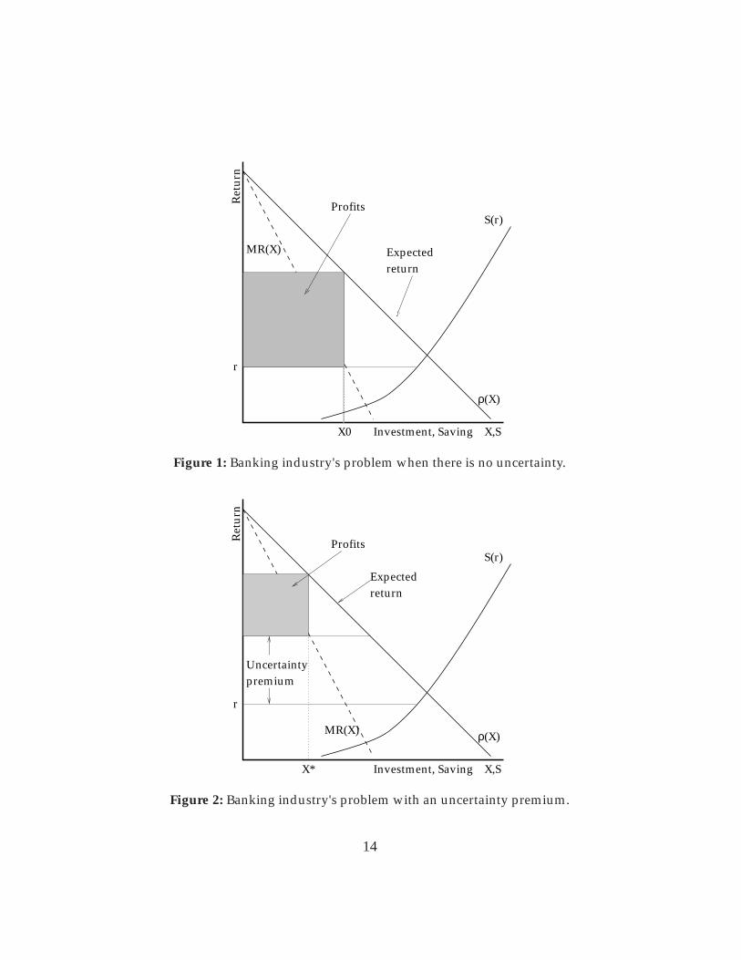
try's profits. The banking industry's problem is shown graphically in fig-

ure 1. The line marked MR(X) is the bank's marginal revenue from raising

an extra unit of deposits and loaning them out. Because the bank can offer

a deposit contract that pays a certain rate of return of Rc = r, investors'

11

decisions are not affected by their uncertainty. Notice the importance of

the assumption that S(r) > X0(r): the banking industry faces a perfectly

elastic supply curve for funds.

We now relax the assumption that banks can earn negative profits in the

bad state. Instead, we assume that output in the bad state is so low as to

preclude any organization, even the government, from smoothing across

aggregate realizations. As a result, banks will be unable to pay a return

on deposits that is constant across all states. In the bad state, banks will

be able to pay at most a return of �0. Because the pessimistic investor puts

undue weight on the bad state, the banking industry will find it optimal

to pay as high a return as possible in that state, R(!) = �0, and thus realize

zero profits in that state. As a result, Knightian uncertainty adjusted rate

of return equality between the risky and the riskless asset [equation (3)]

requires that, for investors to hold both deposits at the bank and govern-

ment bonds, the return on deposits in the good state, R(!), must satisfy:

R(!) =1

1� �

r

p:(9)

The banking industry must therefore pay a markup over the risk-free rate

to attract investors. Here, because we are assuming that R(!) = �0 =

0, the markup is exactly 1=(1 � �). Because the banking industry only

realizes positive profits in the good state of the world, its problem (7) now

12

becomes:

maxX

pX[�(!;X)� R(!)]; subject to: X < S(r).(10)

Here R(!) is as defined in equation (9) above. The solution to this problem

is a level of investment X? that satisfies:

�(!;X?) +X?@�(!;X?)

@X= R(!); or, from (9):(11)

=1

1� �

r

p:

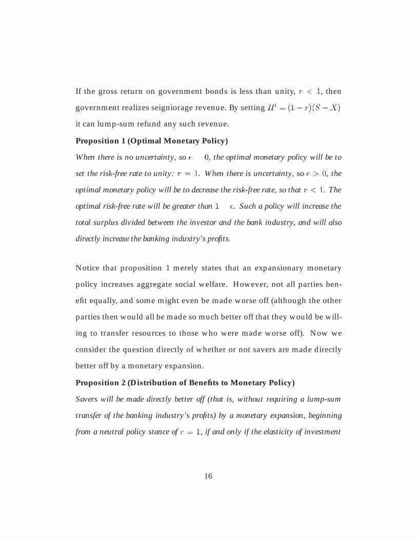
This equation implicitly defines the amount invested as a function of the

risk-free rate, X?(r). The effect of uncertainty on the banking industry is

displayed in figure 2. Notice immediately that when investors are un-

certain, so that � > 0, the amount invested falls below the optimum:

X?(r) < X0(r) for the same level of r. Also, notice that profits (the shaded

area in each diagram) fall as uncertainty rises. In essence, uncertainty in-

creases the cost of funds of banks. By lowering the risk-free rate, the gov-

ernment can force investors to reshuffle their portfolios to contain more

of the risky asset. Such a policy will lower the cost of funds and result in

increased profits to the banking industry.

13

(X)ρ

Expectedreturn

X,S

r

Ret

urn

S(r)

MR(X)

Investment, SavingX0

Profits

Figure 1: Banking industry's problem when there is no uncertainty.

(X)ρ

Uncertaintypremium

Expectedreturn

X,S

r

Ret

urn

S(r)

Investment, Saving

Profits

X*

MR(X)

Figure 2: Banking industry's problem with an uncertainty premium.

14

4 Unconditional Government Monetary Policy

We assume that the government will act to maximize a social welfare func-

tion that sums the banking industry's profits and the investor's utility with

equal weights, netting out the surplus-shifting effects of monetary policy.

Changes in r change the surplus claimed by banks relative to that held by

the investor, as well as changing the investor's optimal portfolio. It is this

latter effect that affects total economy-wide surplus.

The government sells S �X bonds in the first period and pays out a total

of r(S � X) in the second period. The government has a riskless storage

technology that pays a unit return in all states. The government can then

pay a greater or lower return than this “natural” rate on its bonds. If it pays

a higher return, it must levy taxes to pay for the return on its bonds above

the technologically-determined rate. If it pays a lower return, it realizes

revenue, which we assume is refunded lump-sum. We refer to a policy

of depressing the risk-free rate below the natural rate as an expansionary

monetary policy.

The government can make lump-sum transfers (taxes if negative) of H1(!)

in the second period. Thus the government's budget constraint is:

(1� r)(S �X)�H1 � 0:(12)

15

If the gross return on government bonds is less than unity, r < 1, then

government realizes seigniorage revenue. By setting H1 = (1� r)(S �X)

it can lump-sum refund any such revenue.

Proposition 1 (Optimal Monetary Policy)

When there is no uncertainty, so � = 0, the optimal monetary policy will be to

set the risk-free rate to unity: r = 1. When there is uncertainty, so � > 0, the

optimal monetary policy will be to decrease the risk-free rate, so that r < 1. The

optimal risk-free rate will be greater than 1 � �. Such a policy will increase the

total surplus divided between the investor and the bank industry, and will also

directly increase the banking industry's profits.

Notice that proposition 1 merely states that an expansionary monetary

policy increases aggregate social welfare. However, not all parties ben-

efit equally, and some might even be made worse off (although the other

parties then would all be made so much better off that they would be will-

ing to transfer resources to those who were made worse off). Now we

consider the question directly of whether or not savers are made directly

better off by a monetary expansion.

Proposition 2 (Distribution of Benefits to Monetary Policy)

Savers will be made directly better off (that is, without requiring a lump-sum

transfer of the banking industry's profits) by a monetary expansion, beginning

from a neutral policy stance of r = 1, if and only if the elasticity of investment

16

X?(r) exceeds 1=�:

�@X?(r)

@r

r

X?(r)

����r=1

�1

�:

Notice that monetary expansions are thus more likely to directly benefits savers at

larger values of the uncertainty parameter �.

Finally, we consider directly the expected profits of the banking industry

as a whole before the uncertainty parameter has been realized.

Proposition 3 (Banking Industry Profits)

Consider two economies with identical distributions of the uncertainty parameter,

a(�). In the first economy the government sets the risk-free rate to the technolog-

ical rate of return to storage, r = 1, under all realizations of the uncertainty

parameter. In the second economy, the government sets the risk-free rate only af-

ter observing the uncertainty parameter, following an interest-rate policy of r(�).

The policy satisfies 1 � � � r(�) � 1 and also S(r(�)) � X?(r(�)), all �. The

banking industry will make greater expected profits in the second economy than

in the first. Total expected social surplus will be greater in the second economy

than in the first, although without lump-sum transfers between banks and savers,

savers may be worse off.

17

5 Conditional Monetary Policies

In proposition 1 above we established that an expansionary monetary pol-

icy increases the total surplus divided between the investor and the bank-

ing industry (modeled as a representative monopolist); furthermore, a

monetary expansion directly increases the bank's profits. In this section

we expand the range of possible monetary policies to include state contin-

gent values for the return on bonds. Thus the government may, for exam-

ple, commit to an expansion only in the bad state of the world. We show

that this class of policies, if chosen correctly, will also be Pareto-improving.

Therefore, the mere presence of a monetary authority with the right kind of

state-contingent monetary policy will have all of the beneficial effects dis-

cussed in the previous section. However, unless the bad state is realized,

the monetary authority will not move the risk-free rate away from unity. If

the bad state is very unlikely, the monetary authority will almost certainly

be, ex post, passive.

A contingent monetary policy is a choice of rates-of-return on the govern-

ment bond in each state, r(!). We consider only the class of policies in

which the government sets the return on the government bond equal to

unity in the good state, and to some lower rate in the bad state. That is,

the government does nothing in the good state (since a return of unity is

the technologically determined return on the storage technology), and en-

18

gineers a monetary expansion in the bad state. We show that such a policy

is equivalent (with an appropriate change of variables) to an unconditional

policy of the type studied in the previous section.

Monetary policy (in the restricted class that we are studying here) boils

down to a choice of rate of return on the government bond in the bad

state: r(!). The return in the good state is assumed to be unity: r(!) = 1.

Thus the investor's problem (5) becomes:

(13) maxS;X

� (1� S)

+ minfq(!);1�q(!)g2P�

nq(!)[(S �X) +R(!)X]

+ [1� q(!)][r(!)(S �X) +H1(!)]o:

Here, as before, we are assuming that �0 = 0 and so R(!) = 0, for simplic-

ity. In the bad state the government will realize some seigniorage revenue,

which is then refunded lump-sum to the investor via H1(!), determined

by the government's budget constraint (12). In the good state, the govern-

ment does not manipulate the return on bonds, so realizes no seigniorage

revenue.

For both assets to be held in positive amounts, the banking industry must

19

pay a return in the good state, R(!), that satisfies a rate of return equation:

q?(!)R(!) = q?(!) + [1� q?(!)]r(!):(14)

Here q?(!) is the solution to the minimization problem in (13) above; it is

the most pessimistic distribution in P�, given the agent's choices. As we

saw above, the most pessimistic distribution in P� is the one that weights

that bad state the most, and the good state the least:

q?(!) = (1� �)p:

Compare condition (14) to (3), the rate-of-return equality condition when

the government pursues an unconditional monetary policy. We will show

that, within a feasible range, a conditional policy r(!) is equivalent to an

unconditional policy r. Let ru denote an unconditional return on bonds

that produces a desired equilibrium. The allocations associated with this

desired equilibrium, fS(ru); X?(ru)g, may be mimicked by a conditional

policy r(!) that, in turn, leads banks to pay the same returns fR(!); R(!)g.

If we continue to assume, for simplicity, that �0 = 0, and so R(!) = 0, then,

from equation (3):

R(!) =ru

(1� �)p:

Given the conditional policy r(!), from equation (14), we can calculate

20

that:

R(!) = 1 +

�1

q?(!)� 1

�r(!):

The return on the risky asset (that is, uninsured deposits at the bank) in the

good state, R(!), is the same if the conditional monetary policy satisfies:

r(!) =ru � p(1� �)

1� p(1� �):(15)

Because negative gross interest rates are not allowed, the smallest uncon-

ditional interest rate that may be mimicked is:

ru = (1� �)p:

This is below the lowest possible optimal choice of the unconditional risk-

free rate, 1 � �. (See proposition 1 above.) Thus the allocation associated

with the optimal choice of unconditional monetary policy is always avail-

able with a conditional monetary policy of the kind we have outlined here.

Thus, in reacting to a level of uncertainty � > 0, the government may use

either an unconditional monetary policy or a conditional monetary pol-

icy. From equation (15), it is clear that if the government chooses to use

a conditional monetary policy, and the bad state is realized, the monetary

expansion will be greater than if the government had chosen an uncondi-

21

tional monetary policy.

6 Implicit Government Guarantees of the Bank-

ing Industry

Governments often, either explicitly or implicitly, guarantee the safety and

soundness of their national banking industries. Investors feel confident

that certain classes of assets (e.g. deposits at banks) are backed by the gov-

ernment. Investors may also believe that certain ostensibly risky assets

are also, in reality, backed by the government, e.g. equity in an institution

considered to be “too big to fail” or “too embarrassing to fail.” The degree

to which any particular institution is thought to be protected, expressed as

a probability of being bailed out in the bad state, will also affect its prof-

itability. Institutions that are perceived as being more likely to be bailed

out will pay a lower cost of funds than those perceived to be less likely

to be bailed out. Finally, investors may believe that the government will

undertake a wholesale support of many different types of risky assets if

they are threatened by “systemic risk” or “contagion.” Investors, in short,

may trust that many classes of risky assets are implicitly protected by the

government from aggregate shocks.

We can model such an implicit guarantee here by allowing the government

22

to fund the banking industry directly if the bad state of nature is realized.

The banking industry as a whole will continue to make zero profits in

the bad state, but investors will realize more than the pure liquidation

value of the institutions. The government raises seigniorage revenue with

a monetary expansion in the bad state, and then instead of refunding this

revenue lump-sum, it differentially rewards holders of the risky asset.

We shall, it turns out, be able to restrict our attention to a slight generaliza-

tion of the class of conditional monetary policies considered in the previ-

ous section. As before, the government does not distort the rate-of-return

to bonds away from unity in the good state, and engineers a monetary ex-

pansion only if the bad state is realized. Now however, the government

will no longer refund the resulting seigniorage revenue lump-sum, but

will use it to fund the banking industry's claimants directly.

Recall from the government's budget constraint (12), that its total seignior-

age revenue from a monetary expansion, that is, setting a state-contingent

rate of return on government bonds less than unity, in state ! is:

F (!) = [1� r(!)](S �X):

Here S and X represent the representative household's choices of total

savings and holdings of the risky asset. These choices will be affected by

the conditional monetary policy that the government chooses. Assume

23

that seigniorage revenue F is completely distributed, pro rata, to holders

of the risky asset. Thus, in the bad state, the risky asset no longer earns

zero, but rather:

R(!) =F (!)

X; or:

=[1� r(!)](S �X)

X; if S > X .(16)

Assume that, as always, returns in the good state exceed returns in the bad

state, so that R(!) = R(!), despite the government's implicit guarantee.

A monetary policy that combines monetary expansions with direct fund-

ing of the risky asset in bad times will act like a stronger monetary expan-

sion without direct funding (that is, without an implicit guarantee). If the

government chooses a policy of setting the return on bonds to r? < 1 in

the bad state without a guarantee policy, it would be able to achieve the

same results with a policy of setting the return on bonds to r?? > r? with

a guarantee policy. To see this, note that the banking industry must pay a

return in the good state of:

q?R(!) + (1� q?)R(!) = q? � 1 + (1� q?)r(!);(17)

where: q? = (1� �)p; and:

R(!) =[1� r(!)](S �X)

X; if S > X .

As the guarantee amount R(!) increases, the uncertainty premium that

24

the banking industry has to pay falls. Compare the rate-of-return equation

with the guarantee to the one without it, that is, equation (17) to equation

(14). By providing a guarantee the government gets some extra portfolio

bang for its monetary expansion buck.

Although an (implicit or explicit) guarantee policy will in general increase

the expected profits of the banking industry, the banking industry will

continue to fare very poorly in the bad state. Banks realize the extra profits

only if the good state is realized. Next, note that in our analysis there are

no moral hazard considerations to degrade the benefits of a government

guarantee policy. Here, by funding the system in bad times at the expense

of bond holders, the government causes investors to readjust their port-

folios more sharply than with a pure monetary expansion. If investors

had some costly monitoring duties, then such implicit guarantees would

weaken their incentive to properly monitor financial institutions and, ulti-

mately, borrowers.

Finally, consider an intermediary institution that financial markets expect

will be bailed out in the bad state only with probability �. The greater

�, the “closer” the institution is to the government. For example, a large

money-center bank might be seen as a high-� institution, while a small

finance company might be seen as a low-� institution. Consider a single

institution, too small to individually affect the equilibrium levels of aggre-

gate savings and investment S andX . This institution is assigned a bailout

25

probability of �i. Using the augmented rate-of-return equality condition,

equation (17) above, we can determine what return the institution would

have to promise, in the high state, in order to attract deposits, Ri(!):

Ri(!) = �1� q?

q?R(!)�i +

�1 +

1� q?

q?r(!)

�:

As in equation (17) above, q? is the Knightian-uncertainty adjusted prob-

ability of the good state, and R(!) is the return on the risky asset (unin-

sured bank deposits), assuming that the institution is bailed out. Other-

wise, investors anticipate salvaging nothing from their investment in the

bad state. Notice immediately that the return institutions must promise,

Ri(!), is decreasing in the probability of a bailout, �i. However, all insti-

tutions, even those for whom markets estimate no probability of a bailout

(� = 0), benefit from the government's policy of decreasing the risk-free

rate in bad times; that is, of specifying r(!) < 1.

7 Conclusion

In this paper we augmented our model of uncertainty-driven financial

crises to consider how optimal monetary responses would affect the prof-

its of the banking industry. We concluded that optimal monetary policy

responses to uncertainty-led financial crises, which are always expansions,

26

increased expected profits in the banking industry. We further considered

monetary policies that took the form of a conditional monetary expansion,

in which the government reduces the rate paid on its bonds only in clearly

bad economic times. We showed that policies of this kind can always re-

capture the allocations associated with unconditional monetary policies

(although in the companion paper we show that only a fiscal policy can

recapture the first-best allocations). Finally, we showed that monetary

policies combined with an implicit guarantee were more effective at al-

tering investors' portfolio choice than monetary policies alone (in which

the seigniorage revenue was refunded lump sum to investors), and that

financial intermediaries that are perceived by investors as “close” to the

government–that is, more likely to be bailed out by the government in bad

times–benefit more from monetary policy through a lower cost of funds.

Such guarantee policies increase banking industry profits ex ante, and ex

post if the good state is realized.

The government, in our paper, acts to maintain economic growth and sta-

bility by minimizing the number of worthwhile projects that are starved

of capital. A monetary policy that maintains output in the face of uncer-

tainty will, almost as a side-effect, subsidize the banking industry. Such a

subsidy results in a lower cost of funds for banks, possibly giving them a

competitive advantage over intermediaries that are viewed as less closely

tied to government policy.

27

Appendix

Proof of Proposition 1

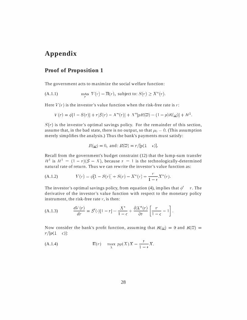
The government acts to maximize the social welfare function:

maxr

V (r) + �(r); subject to: S(r) � X?(r).(A.1.1)

Here V (r) is the investor's value function when the risk-free rate is r:

V (r) = �[1� S(r)] + r[S(r)�X?(r)] +X?[pR(!) + (1� p)R(!)] +H1:

S(r) is the investor's optimal savings policy. For the remainder of this section,assume that, in the bad state, there is no output, so that �0 = 0. (This assumptionmerely simplifies the analysis.) Thus the bank's payments must satisfy:

R(!) = 0; and: R(!) = r=[p(1� �)]:

Recall from the government's budget constraint (12) that the lump-sum transferH1 is H1 = (1 � r)(S � X), because r = 1 is the technologically-determinednatural rate of return. Thus we can rewrite the investor's value function as:

V (r) = �[1� S(r)] + S(r)�X?(r) +r

1� �X?(r):(A.1.2)

The investor's optimal savings policy, from equation (4), implies that �0 = r. Thederivative of the investor's value function with respect to the monetary policyinstrument, the risk-free rate r, is then:

dV (r)

dr= S0(�)[1 � r] +

X?

1� �+@X?(r)

@r

�r

1� �� 1

�:(A.1.3)

Now consider the bank's profit function, assuming that R(!) = 0 and R(!) =r=[p(1� �)]:

�(r) = maxX

p�(X)X �r

1� �X:(A.1.4)

28

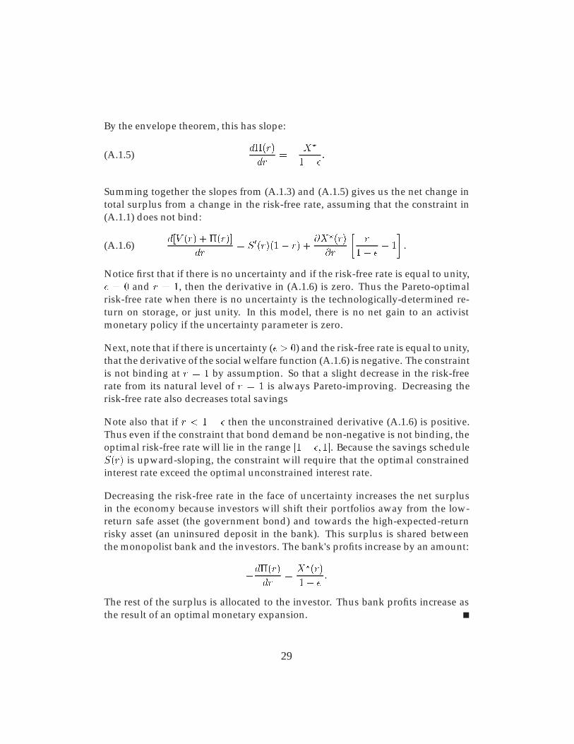
By the envelope theorem, this has slope:

d�(r)

dr= �

X?

1� �:(A.1.5)

Summing together the slopes from (A.1.3) and (A.1.5) gives us the net change intotal surplus from a change in the risk-free rate, assuming that the constraint in(A.1.1) does not bind:

d[V (r) + �(r)]

dr= S0(r)(1 � r) +

@X?(r)

@r

�r

1� �� 1

�:(A.1.6)

Notice first that if there is no uncertainty and if the risk-free rate is equal to unity,� = 0 and r = 1, then the derivative in (A.1.6) is zero. Thus the Pareto-optimalrisk-free rate when there is no uncertainty is the technologically-determined re-turn on storage, or just unity. In this model, there is no net gain to an activistmonetary policy if the uncertainty parameter is zero.

Next, note that if there is uncertainty (� > 0) and the risk-free rate is equal to unity,that the derivative of the social welfare function (A.1.6) is negative. The constraintis not binding at r = 1 by assumption. So that a slight decrease in the risk-freerate from its natural level of r = 1 is always Pareto-improving. Decreasing therisk-free rate also decreases total savings

Note also that if r < 1 � � then the unconstrained derivative (A.1.6) is positive.Thus even if the constraint that bond demand be non-negative is not binding, theoptimal risk-free rate will lie in the range [1� �; 1]. Because the savings scheduleS(r) is upward-sloping, the constraint will require that the optimal constrainedinterest rate exceed the optimal unconstrained interest rate.

Decreasing the risk-free rate in the face of uncertainty increases the net surplusin the economy because investors will shift their portfolios away from the low-return safe asset (the government bond) and towards the high-expected-returnrisky asset (an uninsured deposit in the bank). This surplus is shared betweenthe monopolist bank and the investors. The bank's profits increase by an amount:

�d�(r)

dr=

X?(r)

1� �:

The rest of the surplus is allocated to the investor. Thus bank profits increase asthe result of an optimal monetary expansion.

29

Proof of Proposition 2

Using the results from the proof of proposition 1 above, notice that the slope ofthe representative saver's value function is:

dV (r)

dr= S0(�)(1 � r) +

X?

1� �+@X?

@r

�r

1� �� 1

�:

At r = 1 this becomes:

dV (r)

dr

����r=1;�>0

=X?

1� �+@X?

@r

�1

1� �� 1

�:

This may be rewritten as:

dV (r)

dr

����r=1;�>0

=X?

1� �

�1 + �

@X?

@r

1

X?

�:

For the saver to benefit directly from a decrease in the risk-free rate, this slope mustbe negative. This is the case if and only if:

�@X?

@r

1

X?

����r=1

>1

�:

This is more likely to hold if � is large.

Proof of Proposition 3

From proposition 1 above we know that, along each realization of the uncertaintyparameter �, the banking industry will make greater profits and the total socialsurplus will be greater if the government decreases the risk-free rate in the faceof uncertainty. In particular, if the government does not alter the risk-free rate, itrisks an uncertainty-led financial crisis. Proposition 2 delivers the distributionalcomponents of the proposition.

30

References

Epstein, L. G. and T. Wang (1994). Intertemporal asset pricing underKnightian uncertainty. Econometrica 62(2), 283–322.

Gilboa, I. (1987). Expected utility with purely subjective non-additiveprobabalities. Journal of Mathematical Economics 16(1), 65–88.

Gilboa, I. and D. Schmeidler (1989). Maxmin expected utility with non-unique prior. Journal of Mathematical Economics 18(2), 141–53.

Kwast, M. and W. Passmore (1999). The subsidy provided by the federalsafety net: Theory and evidence. Manuscript, Board of Governors ofthe Federal Reserve System.

Lehnert, A. and W. Passmore (1999). Pricing systemic crises: Monetaryand fiscal policy when savers are uncertain. Forthcoming, Financeand Economics Discussion Series, Board of Governors of the FederalReserve System, Washington DC.

Liu, W. (1999). Heterogeneous agent economies with Knightian uncer-tainty. Manuscript, Department of Economics, University of Wash-ington, Seattle.

Schmeidler, D. (1989). Subjective probability and expected utility with-out additivity. Econometrica 57(3), 571–587.

Whalen, G. (1997). The competitive implications of a safety-net subsidy.Economics Working Paper 97-9, Office of the Comptroller of the Cur-rency.

31