The Assessment of Fit in theClass of Logistic Regression

Models:

A Pathway out of the Jungleof Pseudo-R²s

Dr. Wolfgang LangerMartin-Luther-Universityof Halle-WittenbergInstitute of Sociology 2000

Contents:

� 1. What is the problem?� 2. Summary of the econometric Monte-Carlo

studies for Pseudo-R2s� 3. The generalization of the McKelvey-Zavoina

Pseudo-R2 for multinomial logits� 4. An application in an election study of East

German pupils� 5. What’s to do in future methodological

studies?

1. What is the problem ?

Situation now:� An increasing number of people uses logistic

models for qualitative dependent variables.

� There is no general agreement on how to assessthe fit corresponding to practical significance.

� Where is the pathway out of the jungle of thepseudo-coefficients of determination?

Amemiya (1981):Recommendations

� 1. There is not any universial pseudocoefficient of determination.

� 2. Most of the Pseudo-R²s have values outsidethe range of [0;1]. They are not completelystandardized.

� 3. Assessing the model fit you have to use 2or 3 Pseudo-R²s basing on differentconstruction criteria.

What is the situation now ?

J.Scott Long: (1997):- Regression Models for Categorical and Limited

Dependent Variables. SAGE - (2000): Scalar Measures of Fit for Regression

Models. (http://www.indiana.edu/~jsl650/ )

1.He presents a lot of Pseudo-R2s discussed ineconometric literature.

2.He recommends the McKelvey-Zavoina Pseudo-R2 as the best fit measure for binary and ordinalprobit / logit models.

2.Summary of the econometric Monte-Carlostudies for Pseudo-R2s

� Econometricians have made a lot ofMonte-Carlo studies in the early 90s:- Hagle & Mitchell 1992- Veall & Zimmermann 1992, 1993, 1994- Windmeijer 1995

� They have systematically tested the mostcommon Pseudo-R² for binary and ordinalprobit / logit models

How does a Monte-Carlo simulation studywork?

� 1. You have to generate 100 data sets with amultinormal density and a prescribedmultiple correlation. Then you have tomanipulate systematically the sample sizeand the multiple correlation.

� 2. You have to estimate the multiple linearregression models for each cell of yourdesign.

� 3. You have to dichotomize your dependentvariable using systematically differentcutpoints.

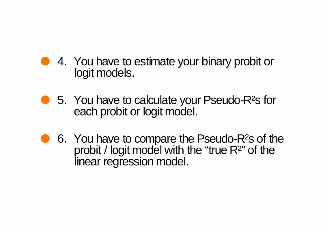
� 4. You have to estimate your binary probit orlogit models.

� 5. You have to calculate your Pseudo-R²s foreach probit or logit model.

� 6. You have to compare the Pseudo-R²s of theprobit / logit model with the “true R²” of thelinear regression model.

Which Pseudo-R²s have been tested?

� Likelihood-based measures: - Maddala / Cox-Snell Pseudo-R²- Cragg-Uhler / Nagelkerke Pseudo-R²

� Log-Likelihood-based measures:- McFadden Pseudo-R²- Aldrich-Nelson Pseudo-R²- Aldrich-Nelson Pseudo-R² with the

Veall-Zimmermann correction� Basing on the estimated probabilities:

- Efron / Lave Pseudo-R²� Basing on the variance decomposition of the

estimated Probits / Logits:- McKelvey-Zavoina Pseudo-R²

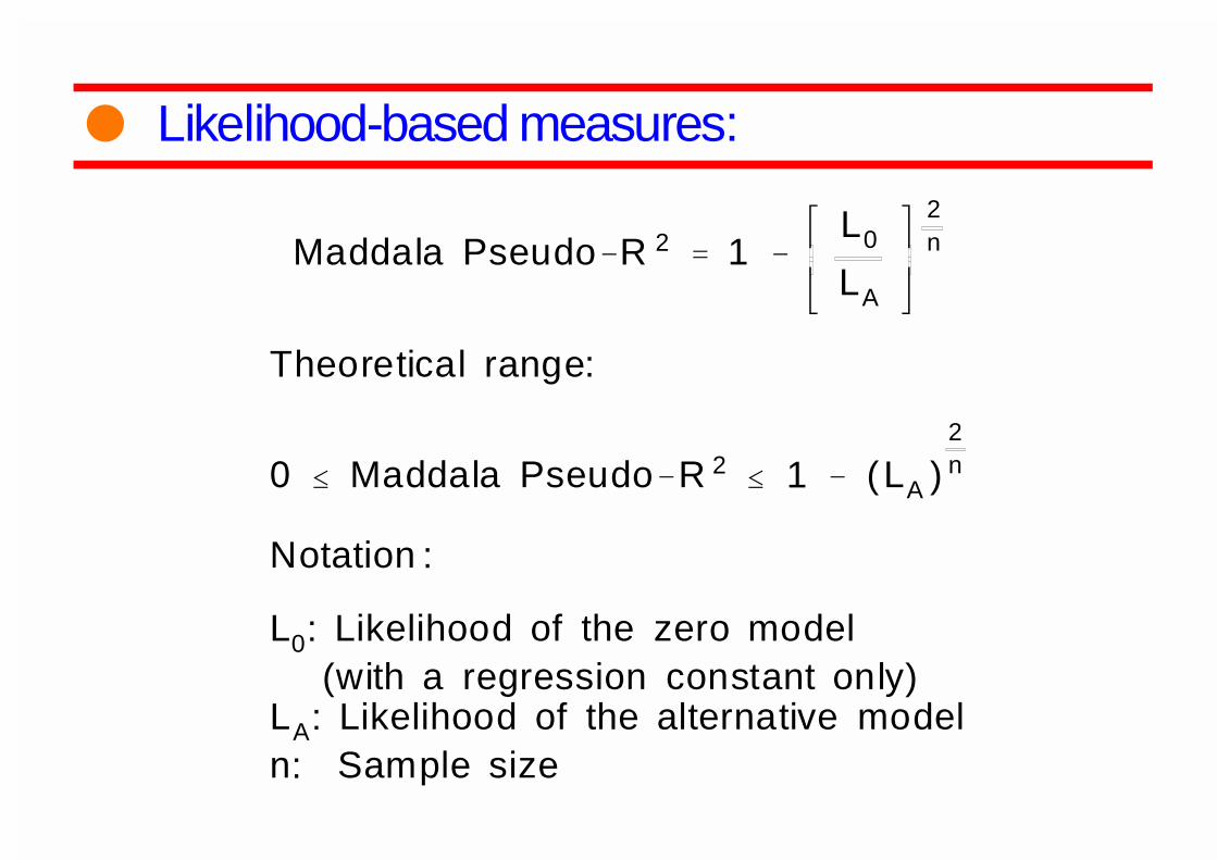
Maddala Pseudo�R 2� 1 �

L0

LA

2n

Theoretical range:

0 � Maddala Pseudo�R 2� 1 � (LA )

2n

Notation :

L0: Likelihood of the zero model(with a regression constant only)

LA: Likelihood of the alternative modeln: Sample size

� Likelihood-based measures:

Cragg�Uhler Pseudo�R 2�

LA

2n

� L0

2n

1 � L0

2n

Theoretical range:

0 � Cragg�Uhler Pseudo�R 2� 1

Standardization of the Maddala Pseudo�R 2

by its own maximum .

McFadden Pseudo�R 2� 1 �

ln L A

ln L0

Theoretical range:

0 � McFadden Pseudo�R 2� 1

It does not reach its maximum of 1 !

Rule of Thumb: 0.20 � McFadden Pseudo�R 2� 0.40

The model has an excellent fit ! (McFadden 1979,307)

Notation :

lnLA: Log�Likelihood of the alternative modellnL0: Log�Likelihood of the zero model

� Log-Likelihood-based measures:

For Probits:

Aldrich�Nelson Pseudo�R2�

LR��2(MA)

LR��2(MA) � n

(MA)

�

2�(lnLA � lnL0)

2� (lnLA � lnL0) � n(MA)

For Logits:

Aldrich�Nelson Pseudo�R2�

LR��2

(MA)

LR��2(MA) � (n(MA)�3.29)

�

2�(lnLA � lnL0)

2�(lnLA � lnL0) � (n(MA)�3.29)

Theoretica l range :

Probits : 0 � Aldrich�Nelson Pseudo�R 2�

�2 � lnL0

n � 2 � lnL0

Logits : 0 � Aldrich�Nelson Pseudo�R 2�

�2 � lnL0

3.29 � n � 2 � lnL0

The A�N Pseudo�R 2 depends on the number and theproportions of the categories of the dependent variables!

You can easily see this at the formula of the log�like lihoodof the zero model:

ln L0 � �

K

k�1nk � ln

n k

n

Notation :nk: Number of cases of category k of the dependent variablen: Sample sizeln: Logarithmus naturalis 3.29: �

2 of the Logistic PDF

Veall�Zimmermann correction of theAldrich�Nelson Pseudo�R 2:

It is standardized by its own reachable maximum dependingon k�categories and their proportions �� range [0 ;1]

For Probits:

Aldrich�Nelson Pseudo�R 2V&Z �

2�(lnLA � lnL0 )

2� (lnLA � lnL0 ) � n

�2� lnL0

n � 2� lnL0

For Logits :

Aldrich�Nelson Pseudo�R 2V&Z �

2� (lnLA � lnL0 )

2� (lnLA � lnL0 ) � 3.29�n

�2� lnL0

3.29�n � 2�lnL0

Lave / Efron Pseudo�R 2� 1 �

�

n

i�1( Y i � p i )

2

�

n

i�1( Y i � Y ) 2

, with Y �1n

� �

n

i�1Y i

Notation:

Y i: Value of the dependent variable in case ip i: Estim ated probability for Y�1 in case i

Y: Observed proportion of category "1"of the dependent variable

� Basing on the estimated probabilities:

McKelvey�Zavoina Pseudo�R2�

SSRegression

SSErrors � SSRegression

(For PROBITs) �

�

n

i�1( y� � y�)2

(n�1.0) � �

n

i�1( y� � y�)2

� Basing on the variance decomposition of the estimatedProbits / Logits

McKelvey�Zavoina Pseudo�R2�

SSRegression

SSErrors � SSRegression

(For LOGITs) �

�

n

i�1( y�i � y�)2

(n�3.29) � �

n

i�1( y�i � y�)2

N o t a t i o n :

y ��

i : E s t i m a t e d L o g i t / P r o b i t o f c a s e i( t h e l i n e a r p r e d i c t o r )

1 . 0 : �2 o f t h e n o r m a l P D F

3 . 2 9 : �2 o f t h e l o g i s t i c P D F

Theoretical range: [ 0 ; 1]

Results of the Monte-Carlo-Studies Corresponding to binary and ordinal probits / logits:

� The McKelvey-Zavoina Pseudo-R² is the bestestimator for the “true R²s” of the OLSregression.

� The Aldrich-Nelson Pseudo-R² with the Veall-Zimmermann correction is the bestapproximation of the McKelvey-ZavoinaPseudo-R².

� Lave / Efron, Aldrich-Nelson, McFadden andCragg-Uhler Pseudo-R² severely underestimatethe “true R²”.

(1) lnP2i

P1i

� ß021� �

K

k�1ßk21

xki� �21

(2) lnP3i

P1i

� ß031� �

K

k�1ßk31

xki� �31

Assumptions for the error terms �k1:

1. �21 and �31 are stochastically independent.2. �21 and �31 are identically distributed.(I ID�Assumption : Hensher &Johnson 1981, 154)

Estimation equations of a multinomial logit model with 3 alternatives:

3. The generalization of the McKelvey&ZavoinaPseudo-R²s for multinomial logits

What is really a multinomial logit (MNL)?

� It is a nonlinear multi-equation model.� The error terms �21 and �31 are independent and

identically distributed.� Therefore you can separately calculate the

McKelvey-Zavoina Pseudo-R² for each equation/ comparison of alternatives !

� Resulting options:- .1 Simultaneous estimation with the MNL- .2 Separate estimation of binary logistic

regression models for each comparison(Begg & Gray 1984)

4.An application in an election study of EastGerman students (Sachsen-Anhalt 1998)

� Social Democratic Party (SPD)

� Christian Democratic Union (CDU)

� Party of Democratic Socialism (PDS, Post-Communist Party)

� Free Democratic Party (FDP)

� The Green Party / Alliance 90 (B90)

� Right extremist parties (DVU, REP, NPD)

Dependent variable:

Which party do you prefer to vote for ?

Alternatives: (one vote only)

• AGE in years• GENDER: boys vs. girls• SCHOOL TYPE: Secondary school, GRAMMAR school,

VOCATIONAL school • Internal and external political EFFICACY • Perceived influence of the peers on the vote (PEERS)• Perceived influence of the parents on the vote

(PARENTS)• Perceived influence of the media on the vote (MEDIA)• Perceived influence of the teachers on the vote

(TEACHERS)• Countryside vs. City (LOCATION)

Independent variables:

SPD 46,9%

CDU 19,5%

PDS 12,6%FDP 3,1%

B90 6,9%

DVU/REP/NPD 11,1%

( n = 1894 )

Party preferences of pupils in Sachsen-Anhalt 1998

Table 1: Party preference of pupils in Sachsen-Anhalt 1998. Multinomial Logit Model (LIMDEP 7 NT)

Independentvariables:

Comparison:

CDU vs. SPD

Comparison:

PDS vs. SPD

Comparison:

FDP vs. SPD

Comparison:

B90 vs. SPD

Comparison:DVU,REP,NPD vs. SPD

Logit S.E. Logit S.E. Logit S.E. Logit S.E. Logit S.E.

Constant - 0,577 0,605 - 3,922** 0,755 - 6,387** 1,436 +0,265 0,906 - 6,562** 0,871

AGE - 0,043 0,035 +0,118** 0,042 +0,178* 0,077 - 0,052 0,053 +0,206** 0,047

GENDER +0,511** 0,131 +0,383* 0,154 +0,520 0,285 - 0,0002 0,200 +1,275** 0,188

GRAMMER VOCATIONAL

+0,870**+0,756**

0,2100,296

+0,932**+0,166

0,2540,356

+0,898- 0,214

0,4670,655

+1,082**- 0,388

0,2920,546

- 0,628- 0,327

0,3460,371

EFFICACY - 0,011 0,021 +0,049 0,025 +0,087 0,048 - 0,084** 0,032 +0,109** 0,029

PEERS - 0,031 0,084 +0,024 0,100 +0,060 0,183 +0,062 0,131 +0,838** 0,097

PARENTS +0,026 0,070 +0,062 0,082 - 0,034 0,154 - 0,164 0,111 - 0,488** 0,102

MEDIA - 0,146* 0,066 - 0,117 0,079 - 0,247 0,143 - 0,300** 0,102 - 0,219* 0,086

TEACHERS - 0,072 0,084 - 0,302** 0,108 - 0,226 0,201 - 0,063 0,137 - 0,032 0,108

LOCATION +0,296 0,187 +0,359 0,236 +0,232 0,447 -0,616* 0,304 +0,699** 0,246

Table 2: Comparis on:CDU vs. SPD

Comparis on :PD S vs . SPD

Comparis on :FD P vs . SPD

Comparison:B90 vs. SP D

Comparis on :D VU,REP,N PDvs. SPD

OverallM cKelvey&Zavoina Pseudo R ²

5 ,642 % 10,048 % 15,096 % 18,779 % 34,998 %

Independentvariab les

� -M&Z Ps eudoR ² in %

�-M &Z PseudoR² in %

�-M &Z PseudoR ² in %

� -M&Z PseudoR ² in %

�-M &Z PseudoR² in %

A GE 0,226 3 ,460 5,082 1,473 2 ,913

GENDER 2,053 0 ,595 0,894 0,052 8 ,709

S CH OOL TYP E 2,071 2 ,214 2,661 11,084 8 ,105

EFF ICA CY 0,041 0 ,671 2,205 1,699 2 ,077

P EERS 0,078 0 ,041 0,003 0,027 7 ,466

PA RTENTS 0,026 0 ,000 0,277 0,624 3 ,850

M EDIA 0,701 0 ,706 1,844 2,110 0 ,773

TEA CHERS 0,070 1 ,470 0,774 0,048 0 ,093

LOCA TION 0,308 0 ,446 0,166 1,509 0 ,680

M odel f it:

Likelihood-Ratio �²-Test = 452 ,29 F.G.= 50 � = 0 ,00 n = 1894 lnL M 0 = -2782,79 lnL M A = -2556,64M cFadden-Pseudo R ² = 8 ,127 %T-Test Results of log it estimators: * ) 0 ,01 < � � 0,05 **) � � 0,01

0

5

10

15

20

25

30

35

Delta-McKelvey &

Zavoina Pseudo-R2

CDU PDS FDP B90 DVU / REP / NPD

Vote for party in comparison with alternative SPD

Party preferences of pupils in Sachsen-Anhalt 1998: Overall fits and relative effect sizes of the

independent variables

LOCATION

TEACHERS

MEDIA

PARENTS

PEERS

EFFICACY

SCHOOLTYPE

GENDER

AGE

Comparision the overall fit of the multinomial and binary logit models by their McKelvey-Zavoina Pseudo-R²s

y = 1,117x - 1,229R2 = 0,995

5

10

15

20

25

30

35

40

5 10 15 20 25 30 35

Multinomial Logit

Bin

ary

Lo

git

Comparison of the partial McKelvey-Zavoina Pseudo-R²s of the multinomial and the binary logit models y = 1,025x + 0,037

R2 = 0,979

0

2

4

6

8

10

12

0 1 2 3 4 5 6 7 8 9 10 11 12

Multinomial Logits

Bin

ary

Lo

git

s

5.What’s to do in future methodological studies?

� Researchers have to present the LR-X², the log-likelihoods of their alternative and zero binary orordinal logit models and the sample size.

� ==> You can easily calculate the corrected Aldrich-Nelson Pseudo-R² with these scalars. Then you canrealistically assess the fit of their binary or ordinallogit / probit model.

� Comparing different models you have to adjustMcKelvey-Zavoina Pseudo-R²s for the sample sizeand the number of estimated parameters withoutthe constant (under investigation).

� Bootstrap studies might be helpful to analyse thedistribution of the M-Z Pseudo-R² and to constructits confidence intervals (under investigation).

References:�Aldrich, J.H.& Nelson, F.D. (1984):

Linear probability, logit, and probit models. Newbury Park: SAGE(Quantitative Applications in the Social Sciences, 45)

�Amemiya, T. (1981):Qualitative response models: a survey. Journal of Economic Literature, 21,pp.1483-1536

�Begg, C.B. & Gray, R. (1984):Calculation of polychotomous logistic regression parameters using individualizedregression. Biometrika, 71, pp.11-18

�Cragg, S.G.& Uhler, R. (1970):The demand for automobiles. Canadian Journal of Economics, 3, pp. 386-406

�Efron, B. (1978):Regression and Anova with zero-one data. Measures of residual variation. Journalof American Statistical Association, 73, pp. 113-121

�Hagle, T.M. & Mitchell II,G.E. (1992):Goodness of fit measures for probit and Logit. American Journal of PoliticalScience, 36, 3, pp. 762-784

�Hensher, D.A.& Johnson, L.W. (1981):Applied discrete choice modelling. London: Croom Helm

�Maddala, G.S. (1983):Limited-dependent and qualitative variables in econometrics. Cambridge:Cambridge University Press

�McFadden, D. (1979):Quantitative methods for analysing travel behaviour of individuals: some recentdevelopments. In: Hensher, D.A.& Stopher, P.R.: (eds):Behavioural travelmodelling. London: Croom Helm, pp. 279-318

�McKelvey, R. & Zavoina, W. (1975):A statistical model for the analysis of ordinal level dependent variables. Journal ofMathematical Sociology, 4, pp. 103-20

�Nagelkerke, N.J.D. (1991):A note on a general definition of the coefficient of determination. Biometrika, 78, 3,pp.691-693

�Ronning, G. (1991):Mikro-Ökonometrie. Berlin: Springer

�Veall, M.R. & Zimmermann, K.F. (1992):Pseudo-R2 in the ordinal probit model. Journal of Mathematical Sociology, 16, 4,pp. 333-342

� Veall, M.R. & Zimmermann, K.F. (1994):Evaluating Pseudo-R2's for binary probit models. Quality&Quantity, 28, pp. 151- 164

�Windmeijer, F.A.G. (1995):Goodness-of-fit measures in binary choice models. Econometric Reviews, 14, 1,pp. 101-116

�Zimmermann, K.F. (1993): Goodness of fit in qualitative choice models: review and evaluation. In:Schneeweiß, H. & Zimmermann, K. (eds):Studies in applied econometrics. Heidelberg: Physika, pp. 25-74