The ASIMOV high-speed linkjpg/reps/asimovtr.pdf · The ASIMOV High-Speed Link Jo~ao Pedro Gomes...
70
The ASIMOV High-Speed Link Jo˜ ao Pedro Gomes Victor Barroso Instituto Superior T´ ecnico – Instituto de Sistemas e Rob´ otica Av. Rovisco Pais, 1049-001 Lisboa, Portugal [email protected] April 26, 2005
Transcript of The ASIMOV high-speed linkjpg/reps/asimovtr.pdf · The ASIMOV High-Speed Link Jo~ao Pedro Gomes...
The ASIMOV High-Speed Link
Joao Pedro Gomes Victor Barroso
Instituto Superior Tecnico – Instituto de Sistemas e Robotica
Av. Rovisco Pais, 1049-001 Lisboa, Portugal
April 26, 2005

Contents
Notation iv
Symbols . . . . . . . . . . . . . . . . . . . . . . . . . . . . . . . . . . . . . . . . . iv
Acronyms . . . . . . . . . . . . . . . . . . . . . . . . . . . . . . . . . . . . . . . . v
1 General Overview 1
1.1 Introduction . . . . . . . . . . . . . . . . . . . . . . . . . . . . . . . . . . . . 1
1.2 Systems Description . . . . . . . . . . . . . . . . . . . . . . . . . . . . . . . 2
1.2.1 Acoustic Compatibility and Directivity . . . . . . . . . . . . . . . . . 3
1.2.2 Link Reliability and Complexity Requirements . . . . . . . . . . . . 3
1.2.3 Communication Hardware . . . . . . . . . . . . . . . . . . . . . . . . 4
1.3 Outline of the Report . . . . . . . . . . . . . . . . . . . . . . . . . . . . . . 5
2 Signal Processing Structure 6
2.1 Signal Processing at the Receiver . . . . . . . . . . . . . . . . . . . . . . . . 6
2.1.1 Timing Recovery . . . . . . . . . . . . . . . . . . . . . . . . . . . . . 8
2.1.1.1 Interpolator . . . . . . . . . . . . . . . . . . . . . . . . . . 9
2.1.1.2 Doppler Tracking Considerations . . . . . . . . . . . . . . . 10
2.1.2 Equalization . . . . . . . . . . . . . . . . . . . . . . . . . . . . . . . 11
2.1.2.1 Equalizer Order . . . . . . . . . . . . . . . . . . . . . . . . 12
2.1.2.2 Blind Algorithms . . . . . . . . . . . . . . . . . . . . . . . 13
2.1.2.3 Reference-Driven Algorithms . . . . . . . . . . . . . . . . . 13
2.1.3 Carrier Recovery and Slicing . . . . . . . . . . . . . . . . . . . . . . 14
2.1.3.1 Low-level Slicing for 4-PSK and 8-PSK . . . . . . . . . . . 14
2.2 Signal Processing at the Transmitter . . . . . . . . . . . . . . . . . . . . . . 16
3 Coding 18
3.1 Coder and decoder structure . . . . . . . . . . . . . . . . . . . . . . . . . . 18
3.2 Interleaving . . . . . . . . . . . . . . . . . . . . . . . . . . . . . . . . . . . . 19
3.3 Rotationally-Invariant TCM for M-PSK Constellations . . . . . . . . . . . . 21
3.3.1 TCM Encoder . . . . . . . . . . . . . . . . . . . . . . . . . . . . . . 22
3.3.1.1 16-state TCM: . . . . . . . . . . . . . . . . . . . . . . . . . 23
3.3.2 Link operation with plain 4-PSK and 8-PSK . . . . . . . . . . . . . 24
3.3.3 TCM Decoder . . . . . . . . . . . . . . . . . . . . . . . . . . . . . . 25
i
ii CONTENTS
4 Data Formatting 27
4.1 Frame Structure . . . . . . . . . . . . . . . . . . . . . . . . . . . . . . . . . 27
4.1.1 Frame data . . . . . . . . . . . . . . . . . . . . . . . . . . . . . . . . 28
4.1.1.1 Markers and data scrambling . . . . . . . . . . . . . . . . . 29
4.1.1.2 Interleaving matrices . . . . . . . . . . . . . . . . . . . . . 29
4.1.1.3 Symbol mapping . . . . . . . . . . . . . . . . . . . . . . . . 30
4.1.1.4 Character and bit stuffing . . . . . . . . . . . . . . . . . . . 31
4.2 Layered Processing at the Receiver . . . . . . . . . . . . . . . . . . . . . . . 33
4.2.1 Mapper/Unmapper Reset: . . . . . . . . . . . . . . . . . . . . . . . . 35
4.3 Transmitter and Receiver Configuration . . . . . . . . . . . . . . . . . . . . 36
4.3.1 Frame Parameters (modem.c) . . . . . . . . . . . . . . . . . . . . . . 37
4.3.1.1 Mapping Functions . . . . . . . . . . . . . . . . . . . . . . 38
4.3.1.2 Differential Encoder/Decoder State: . . . . . . . . . . . . . 39
4.3.2 Generic Data Pump Parameters (dpump.c) . . . . . . . . . . . . . . 39
4.3.3 Timing Recovery Parameters (betr.c) . . . . . . . . . . . . . . . . . 40
4.3.4 Carrier Recovery Parameters (psksync.c) . . . . . . . . . . . . . . . 40
4.3.5 Equalization Parameters (equaliz.c) . . . . . . . . . . . . . . . . . 41
4.3.6 Sample Configuration: 4-PSK . . . . . . . . . . . . . . . . . . . . . . 42
4.3.7 Sample Configuration: 4-State TCM . . . . . . . . . . . . . . . . . . 44
5 Software Organization 46
5.1 Software Modules . . . . . . . . . . . . . . . . . . . . . . . . . . . . . . . . . 46
5.1.1 Modem Management and Testing . . . . . . . . . . . . . . . . . . . . 47
5.1.2 Bit/Character Buffer Management . . . . . . . . . . . . . . . . . . . 47
5.1.3 Frame Preambles . . . . . . . . . . . . . . . . . . . . . . . . . . . . . 47
5.1.4 Data Pump . . . . . . . . . . . . . . . . . . . . . . . . . . . . . . . . 47
5.1.4.1 Filtering . . . . . . . . . . . . . . . . . . . . . . . . . . . . 48
5.1.5 Mapping/Unmapping . . . . . . . . . . . . . . . . . . . . . . . . . . 48
5.1.6 Numeric Functions . . . . . . . . . . . . . . . . . . . . . . . . . . . . 48
5.2 Numeric Implementation . . . . . . . . . . . . . . . . . . . . . . . . . . . . . 48
5.3 Compile-time Definitions . . . . . . . . . . . . . . . . . . . . . . . . . . . . . 50
5.3.1 Mapping Functions . . . . . . . . . . . . . . . . . . . . . . . . . . . . 51
5.4 Sample Makefiles . . . . . . . . . . . . . . . . . . . . . . . . . . . . . . . . . 52
5.4.1 Transmitter . . . . . . . . . . . . . . . . . . . . . . . . . . . . . . . . 52
5.4.2 Receiver . . . . . . . . . . . . . . . . . . . . . . . . . . . . . . . . . . 52
A Band-Edge Timing Recovery 53
A.1 Band-Edge Filter Design . . . . . . . . . . . . . . . . . . . . . . . . . . . . . 55
A.2 Matlab Code for Generating Band-Edge Filters . . . . . . . . . . . . . . . . 56
A.3 Fixed-Point Representation . . . . . . . . . . . . . . . . . . . . . . . . . . . 57
A.4 Matlab Code for Computing Filter Parameters . . . . . . . . . . . . . . . . 59

CONTENTS iii
Bibliography 62

Notation
For reference purposes, some of the most common symbols and acronyms adopted in this
report are listed below.
Symbols
Matrices and vectors are denoted by upper-case and lower-case boldface characters, re-
spectively.
[A]i,j ij-th element of matrix A
[v]i i-th element of column vector v
(·)∗ Complex conjugate
(·)T Transpose
(·)H Conjugate transpose (Hermitean)
Re {·} Real part
Im {·} Imaginary part
∗ Convolution
|z| Magnitude of a complex or real number
‖v‖ Vector norm ‖v‖ = (v∗v)1
2
u(t), U(ω) Complex baseband signal in the time and frequency domains
u(t), U(ω) Real passband signal
a(n) Symbol drawn from a complex constellation
a(n), a(n) Symbol estimates at the input and output of a hard decision device (slicer)
δ(·) Dirac delta function (continuous argument) or Kronecker unit impulse (dis-
crete argument)
E {·} Expected value
h(t) Time-invariant received PAM pulse shape
j√−1
L Oversampling factor in a discrete PAM sequence
n Discrete sequence index
Tb PAM signaling interval
τ Continuous delay
ω Continuous or discrete frequency
iv

v
ωc Carrier frequency
x(·) Transmitted signal
y(·) Multipath-distorted received signal
Acronyms
AGC Automatic Gain Control
ASC Autonomous Surface Craft
ASIMOV Advanced Systems Integration for Managing the coordinated operation of
robotic Ocean Vehicles
AUV Autonomous Underwater Vehicle
BETR Band-Edge Timing Recovery
DDS Direct Digital Synthesis
DGPS Differential GPS
DPSK Differential PSK
DQAM Differential QAM
DSP Digital Signal Processor
DFE Decision-Feedback Equalizer
DMA Direct Memory Access
FIR Finite Impulse Response
FSE Fractionally-Spaced Equalizer
FSK Frequency-Shift Keying
GPS Global Positioning System
IF Intermediate Frequency
IIR Infinite Impulse Response
ISI Intersymbol Interference
LFSR Linear-Feedback Shift Register
LFM Linear Frequency Modulation
LMS Least-Mean-Square
LSB Least Significant Bit
MIPS Mega Instructions per Second
MISO Multiple-Input Single-Output
MSB Most Significant Bit
MSE Mean-Square Error
NCMA Normalized Constant-Modulus Algorithm
NLMS Normalized LMS
PAM Pulse Amplitude Modulation
PLL Phase-Locked Loop
PSK Phase-Shift Keying

vi Notation
QAM Quadrature Amplitude Modulation
RLS Recursive Least-Squares
SCS Soft-Constraint Satisfaction
SIMO Single-Input Multiple-Output
SISO Single-Input Single-Output
SLMS adaptive Step-size LMS
TCM Trellis-Coded Modulation
UART Universal Asynchronous Receiver-Transmitter
USBL Ultra-Short Base Line

Chapter 1
General Overview
This report describes the ISR–IST contribution for the high-speed acoustic data link that
was developed as part of the ASIMOV project. This contribution consists of several C
software modules that implement most of the functionality of a modem, from physical-
level synchronization and filtering to top-level data framing. This software was integrated
with ORCA Instrumentation driver modules that interact with a custom-developed board
based on a low-power Texas Instruments fixed-point TMS320C54x DSP.
As the modem software is relatively complex, documenting it from the strict perspec-
tive of software engineering is somewhat inadequate. Accordingly, this report addresses
several issues, such as the transmitter and receiver signal processing structure, data for-
mat, software organization, and software parametrization. Section 1.3 provides an outline
of this report.
1.1 Introduction
One of the main purposes of project ASIMOV is to demonstrate the potential applications
of underwater autonomous vehicles (AUVs) for demanding scientific missions. Several
factors that have hindered the widespread use of AUVs in practical applications can be
traced back to the limited amount of data that can be exchanged in near real time between
a (tetherless) vehicle and a mission control center using acoustic modems. Most notably,
such lack of interactivity prevents end-users from assessing the unfolding of missions, and
re-directing the vehicle when appropriate.
Although acoustic modems use sophisticated signal processing techniques to compen-
sate for severe intersymbol interference (ISI) and other distortions that affect the trans-
mitted waveforms as they propagate through dispersive underwater channels, fundamental
limits restrict the data rates that can be reliably achieved. In general-purpose commercial
acoustic modems, for example, the typical throughput is only 1 or 2Kbps, which is clearly
insufficient for ASIMOV, where a data rate of 30Kbps has been specified for transmission
of compressed images. To overcome this limitation, acoustic transmission always takes
place vertically in the framework of project ASIMOV, thus providing a comparatively
benign communication channel where high data rates are attainable. An Autonomous
1
2 General Overview
Autonomous SurfaceCraft (ASC)
Autonomous UnderwaterVehicle (AUV)
Support Ship
Radio Link
High RateAcoustic Link
(Data)
Low RateAcoustic Link
(Commands/Data)
Low RateAcoustic Link(Commands)
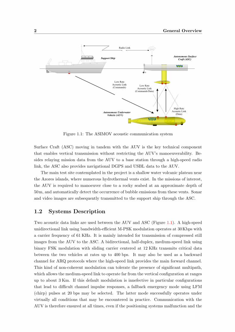
Figure 1.1: The ASIMOV acoustic communication system
Surface Craft (ASC) moving in tandem with the AUV is the key technical component
that enables vertical transmission without restricting the AUV’s manoeuverability. Be-
sides relaying mission data from the AUV to a base station through a high-speed radio
link, the ASC also provides navigational DGPS and USBL data to the AUV.
The main test site contemplated in the project is a shallow water volcanic plateau near
the Azores islands, where numerous hydrothermal vents exist. In the missions of interest,
the AUV is required to manoeuver close to a rocky seabed at an approximate depth of
50m, and automatically detect the occurrence of bubble emissions from these vents. Sonar
and video images are subsequently transmitted to the support ship through the ASC.
1.2 Systems Description
Two acoustic data links are used between the AUV and ASC (Figure 1.1). A high-speed
unidirectional link using bandwidth-efficient M-PSK modulation operates at 30Kbps with
a carrier frequency of 61 KHz. It is mainly intended for transmission of compressed still
images from the AUV to the ASC. A bidirectional, half-duplex, medium-speed link using
binary FSK modulation with sliding carrier centered at 12 KHz transmits critical data
between the two vehicles at rates up to 400 bps. It may also be used as a backward
channel for ARQ protocols where the high-speed link provides the main forward channel.
This kind of non-coherent modulation can tolerate the presence of significant multipath,
which allows the medium-speed link to operate far from the vertical configuration at ranges
up to about 3 Km. If this default modulation is innefective in particular configurations
that lead to difficult channel impulse responses, a fallback emergency mode using LFM
(chirp) pulses at 20 bps may be selected. The latter mode successfully operates under
virtually all conditions that may be encountered in practice. Communication with the
AUV is therefore ensured at all times, even if the positioning systems malfunction and the

1.2 Systems Description 3
exact AUV location is lost.
1.2.1 Acoustic Compatibility and Directivity
Important design considerations involve the acoustic compatibility between the two sys-
tems, as it should be possible to transmit emergency commands to the AUV through
the medium-speed link even when the high-speed link is active in the reverse direction.
Although the operating frequencies for the two subsystems are non-overlapping, this re-
quirement restricts the placement of transducers to avoid pre-amplifier cross-saturation
while retaining a compact mechanical assembly.
The relatively low carrier frequency of 12 KHz used by the medium-speed link ensures
that the acoustic signals suffer moderate absorption while propagating in the water, allow-
ing direct communication between the AUV and a surface vessel over distances of several
kilometers. Naturally, the high availability requirements in this communication link under
significant uncertainty in transmitter/receiver locations can only be met if omnidirectional
transducers are used at all endpoints (ASC, AUV, support ship). The medium-speed link
is based on one of ORCA’s commercially available solutions, and its features will not be
covered in detail here.
Transducer directivity in the high-speed link needs to be carefully considered, as there
is a delicate balance between the accuracy of the positioning systems that ensure a fa-
vorable AUV/ASC configuration and the optimal directivity that minimizes intersymbol
interference and fading in the communication channel. At the AUV, a top-mounted pro-
jector encased in a foam baffle creates an upward-looking directivity pattern whose main
lobe has a width of about 60 degrees. It was experimentally verified that the residual
acoustic energy that reaches the nearby omnidirectional transducer for the medium-speed
link does not saturate the pre-amplifiers. The 61 KHz signal may therefore be rejected
with bandpass filtering, allowing the medium-speed link to remain usable in the downward
direction. Naturally, a transmission to the AUV at 12 KHz will likely corrupt any high-
speed upward transmission, but simultaneous operation of the two links will only occur in
emergency situations.
At the ASC, a foam baffle surrounding the single receiving hydrophone creates a direc-
tivity pattern similar to the one used at the transmitter. To reduce the effects of thruster
and surface noice, both ASC acoustic transducers are mounted on a “torpedo” that is
vertically lowered from the center of the craft to a depth of about 1.5 m (Figure 1.1).
1.2.2 Link Reliability and Complexity Requirements
Since mission-critical data will typically not be transmitted through the high-speed link,
ensuring negligible error probability is not the primary design concern. Bit error rates of
10−4 to 10−3 may be sufficient for a human supervisor to verify that the vehicle operates
as intended based on a sequence of images with a frame rate of about 0.5 Hz. If better
performance is required, an outer layer should be used to code the modem input bit stream,

4 General Overview
ProjectorRS-232
BPFDDSDSP
TI ‘C54x
PowerAmpUART
(a)
Pre Amp/AGC
Hydrophone RS-232
BPFIF Down-Convert
DSPTI ‘C54x
UART
(b)
Figure 1.2: Basic hardware blocks (a) Transmitter (b) Receiver
thus decreasing both the error probability and the effective data rate.
The AUV and ASC house a number of other subsystems for mission planning, guid-
ance and control, positioning, sonar/video imaging, obstacle avoidance, etc. This is not
intended as a dedicated testbed for acoustic transmission, and the resources that have
been allocated to the communication system are somewhat limited. In particular, diver-
sity techniques using multiple projectors/hydrophones have not been contemplated, and
the available digital signal processing hardware was designed with rather stringent power
consumption constraints. Therefore, the unusually high data rates that are required in the
high-speed link are supported primarily by a favorable transmission geometry. Signal pro-
cessing algorithms at the receiver are only meant to compensate for moderate distortions
in the received waveforms.
1.2.3 Communication Hardware
The central component of both the transmitter and receiver is a single-processor board
based on the Texas Instruments TMS320C54x 16-bit fixed-point DSP running at 120 MIPS
(Figure 1.2). At the transmitter, the DSP receives bytes from a UART and calculates the
required phases of the M-PSK signal, which are sent to a frequency synthesizer (DDS) for
actual waveform generation. This signal is bandpass filtered to 61± 15 KHz before being
power-amplified and applied to the projector. The filtering operation distorts the shape
of the original square baseband signaling pulses, and introduces moderate intersymbol
interference that must be compensated upon reception. Although suboptimal from the
perspective of power efficiency, M-PSK modulation was chosen due to the simplicity with
which bandpass waveforms can be generated using a DDS. Presumably, the availibility
of M-QAM constellations would have enabled enhanced performance when using coded
modulation.
At the receiver, an analog front-end removes out-of-band noise components, provides
automatic gain control and downconverts the signal to an intermediate frequency band
between 0 and 30 KHz. After A/D conversion, all subsequent processing is performed by
the DSP. The type of algorithms that may be used are conditioned by the native fixed-
point precision and the internal memory size. Block-processing techniques are not well
suited for this architecture, as no external memory is used for efficiency reasons.
Within the class of M-PSK constellations that are available at the transmitter, it

1.3 Outline of the Report 5
seems unreasonable to expect acceptable (raw) symbol error probabilities with more than
8 constellation points, since this would require excessively high transmit power. To attain
the target rate of 30 Kbps, it was decided to transmit unencoded data at 15 Kbaud using
4-PSK. As discussed in Section 3.3.1, coded data are transmitted at the same baud rate
using an 8-PSK constellation.
1.3 Outline of the Report
The present chapter described some acoustic link specifications and the hardware platform.
The remainder of this report is organized as follows:
Chapter 2 addresses the signal processing blocks and algorithms that are used at the
receiver (and, to a lower extent, at the transmitter) to map baseband waveforms into raw
complex symbols and vice-versa.
The algorithms used for signal-space coding through Trellis-coded modulation are re-
viewed in Chapter 3. This low-level coding layer provides some improvement in output
bit-error rate without sacrificing bandwidth by expanding the signal constellation.
Chapter 4 describes the structure and parameters of data frames. It discusses how data
is formatted in hierarchical units and what mechanisms are available to resynchronize the
decoding process even if some of the symbols in the frame are duplicated or lost at the
receiver.
Finally, Chapter 5 provides an overview of the software modules that comprise the
transmitter and receiver and discusses relevant issues such as the implementation of fixed-
or floating-point arithmetic. It also describes how the programs can be parameterized by
compiler options and provides example makefiles.
Chapter 2
Signal Processing Structure
This chapter describes the signal processing algorithms that are used at the transmitter
and receiver. Naturally, the emphasis will be placed on the latter, which has much more
stringent computational requirements.
Coherent modulation was chosen for the high-rate link, as it is the only signaling
method whose spectral efficiency allows the target data rate of 30 Kbps to be attained
within the available bandwidth. The choice of equalization and synchronization algorithms
was constrained by the computational resources provided by a single Texas Instruments
TMS320C54x 16-bit fixed-point DSP operating at 120 MIPS, which was used to imple-
ment the full receiver with no external memory. Due to the limitations of computational
power and numerical precision, both conventional RLS algorithms and their fast (but nu-
merically sensitive) versions [10] cannot reallistically be implemented on this hardware
platform, although they have been used as benchmarks when analyzing the experimental
data gathered during field tests. Since there is an inevitable tradeoff between the com-
plexity of equalization algorithms and the degree of distortion in the incoming signal that
can be compensated, it is clear that this receiver will only operate reliably under favorable
multipath conditions, such as those observed in vertical channels. The performance of this
receiver is analyzed in [5, 8, 6, 7].
2.1 Signal Processing at the Receiver
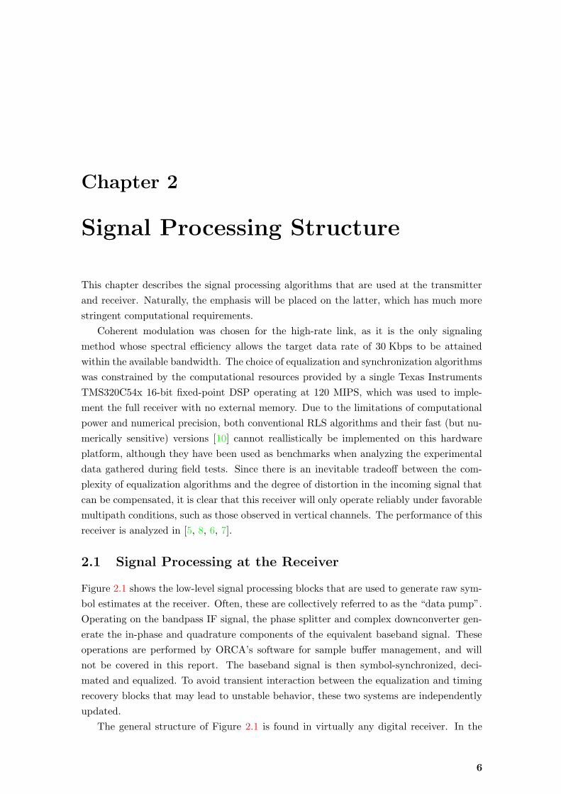
Figure 2.1 shows the low-level signal processing blocks that are used to generate raw sym-
bol estimates at the receiver. Often, these are collectively referred to as the “data pump”.
Operating on the bandpass IF signal, the phase splitter and complex downconverter gen-
erate the in-phase and quadrature components of the equivalent baseband signal. These
operations are performed by ORCA’s software for sample buffer management, and will
not be covered in this report. The baseband signal is then symbol-synchronized, deci-
mated and equalized. To avoid transient interaction between the equalization and timing
recovery blocks that may lead to unstable behavior, these two systems are independently
updated.
The general structure of Figure 2.1 is found in virtually any digital receiver. In the
6

2.1 Signal Processing at the Receiver 7
PhaseSplitter
Interpolator
TimingRecovery
EqualizedSymbol
To MarkerScanning
CarrierRecovery
Equalizer
IF Signal
PSfrag replacements
e−jωcn
e−jθ ejθ
Figure 2.1: Receiver signal processing blocks (data pump)
context of underwater communications, the most widely used receiver architecture was
proposed by Stojanovic [19], and comprises a decision-feedback equalizer (DFE) coupled
with a phase-locked loop (PLL) for carrier recovery. This is often referred to as a sort
of canonical receiver, against which any proposed system should be benchmarked [12, 1].
Computational constraints and the analysis of data collected at the test site have led to the
adoption of algorithms for the ASIMOV receiver that differ from those originally proposed
in [19].
In addition to the core signal processing functions that provide raw symbol estimates
from the received waveform, the ASIMOV receiver is formed by several other blocks,
including signal-space coding, scrambling, and frame/marker synchronization [9]. These
are described in Chapters 3 and 4. Note that the slicer shown in Figure 2.1, and described
in more detail in Section 2.1.3.1, is internal to the data pump. Its purpose is to provide low-
delay preliminary decisions which are needed to adapt both the equalizer and the carrier
recovery loop. Concurrently, the phase-corrected equalizer output is sent to a higher-level
unmapping function which can take into account any underlying code structure to reduce
the output bit error rate at the expense of increased decoding delay.
Sampling Rates: The baseband signal at the interpolator input is sampled at 60 kHz,
i.e., oversampled by a factor of L = 4 relative to the symbol rate1 of 15 kbaud. The signal
is decimated to L = 2 samples per symbol (30 kHz) at the equalizer input, which outputs
estimates at the symbol rate of 15 kHz. All subsequent processing is done at this rate.
To avoid the burden of handling synchronized threads associated with multiple pro-
cessing blocks operating at different speeds, DSP systems commonly optimize throughput
rates by processing data in “batch” mode, where each batch is a collection of consecutive
signal samples that have been buffered into a single unit. By propagation these multisam-
ple vectors instead of the individual signal samples, DSP systems can reduce the overhead
of function calls and task synchronization. This philosophy was adopted in the ASIMOV
1When rotationally-invariant TCM modulation is used in the ASIMOV high-speed link an actual sym-bol is four dimensional and consists of a pair of complex values, each belonging to a standard 8-PSKconstellation. Strictly speaking, the symbol rate is therefore 7.5 kbaud. However, in the context of thecore signal processing system of Figure 2.1 the term symbol will usually be used to denote a complex pointbelonging to a conventional (2D) constellation.

8 Signal Processing Structure
high-speed receiver, whose core signal processing blocks are triggered at symbol rate:
Interpolator: The Farrow interpolator receives vectors of 4 baseband input samples2 and
generates an interpolated sample vector of the same dimension.
Timing Recovery: Band edge filters operate on 4-sample vectors of interpolated sam-
ples. Only one element of every filter output vector is retained, as all subsequent
processing in the timing recovery loop is formallly done at the symbol rate.
Equalizer: The equalizer operates on 2-sample vectors and generates scalar symbol esti-
mates. Notice the slight inconsistency of Figure 2.1, which suggests that the same
set of samples is input to the timing recovery block and the equalizer. In fact, the
former processes the full 4-sample interpolated vector, whereas the latter is fed a
vector decimated by a factor of 2.
Carrier Recovery: The carrier recovery block receives and outputs scalar samples.
As described in Section 3.3.1, for efficiency reasons the Trellis decoder for TCM uses
a block sliding window, and can therefore be thought of as generating vectors of bits.
However, it is triggered at the (TCM) input symbol rate of 7.5 kHz regardless of whether
output bits are actually generated.
2.1.1 Timing Recovery
Very simple timing recovery algorithms may be derived by joint optimization of the optimal
sampling instant and equalizer coefficients [19]. This approach is somewhat unreliable, as it
requires the inclusion of a highly complex equalizer transfer function inside a feedback loop
that may easily become unstable [13]. Therefore, an important practical requirement for
the receiver of Figure 2.1 is that the timing recovery system be independent of the adaptive
equalizer. Moreover, it must be relatively simple and remain effective for any M-PSK
constellation even when the signal suffers from significant intersymbol interference, which
rules out most of the techniques that are commonly used in other digital communication
applications [16]. Based on these criteria, band-edge timing recovery (BETR) was selected
[4, 11].
Let yc(t) be a received PAM signal
yc(t) =∞
∑
k=−∞
a(k)hc(t− kTb) + ηc(t) , (2.1)
where a(k) is the k-th transmitted symbol, hc(t) is the received pulse shape, Tb is the
signaling interval, and ηc(t) denotes additive noise. As detailed in Appendix A, BETR
adjusts the optimum sampling offset τ to iteratively maximize the power of a baud-rate-
sampled sequence E{|yc(nTb+τ)|2}. A block diagram of the system is shown in Figure 2.2.
Fh and Fl are complex bandpass filters centered around the upper and lower band-edge
2As discussed in Section 2.1.1.1, the number of samples that are actually read from the basebandsample buffer may change when wrap-around of the optimal sampling instant occurs. However, thisshould normally be an infrequent event that is of little relevance here.

2.1 Signal Processing at the Receiver 9
ErrorUpdate
InterpolatedInput Loop
FilterSmooth &Normalize
PSfrag replacementsFh(ω)
Fl(ω) (·)∗
↓ L Im{·}
Figure 2.2: Band-edge timing recovery system
frequencies ±rb/2, where rb is the signaling rate. The product of their outputs generates
a signal containing a spectral line at rb, whose phase is to be tracked. This signal is
decimated to one sample per symbol, smoothed and normalized, and its imaginary part
used to drive a loop filter that provides a timing correction. When used in a feedback
configuration, the goal of the timing recovery loop is to drive to zero the error at the input
of the loop filter of Figure 2.2. Further details may be found in Appendix A and in [4, 11].
This processing structure reflects the fact that, if the excess bandwidth in the spectrum
of hc(t) is less than rb/2, then the Tb-periodic BETR cost function has a single nonzero
Fourier coefficient at frequency rb = 1/Tb, in addition to the DC component [13].
In principle, the baud spectral line signal (BSL), i.e., the decimated product of band-
edge filter outputs, could drive the loop filter directly, but then the feedback parameters
would be dependent on the signal power, which is undesirable. As only the phase of the
BSL is relevant, a more robust alternative proposed in [11] is to normalize it to unit mag-
nitude prior to loop filtering. Straightforward generation of a unit-magnitude signal U(n)
from the BSL r(n) as U(n) = r(n)/|r(n)| requires square-root and division operations,
which are rather computationally intensive. A more effective procedure proposed in [11]
first passes r(n) through a first-order lowpass filter to yield the smoothed BSL
R(n) = R(n− 1) + k2
(
r(n)−R(n− 1))
, k2 = 1/1024 , (2.2)
which is then approximately normalized by the iteration
U ′(n) =(
1 + k3 j sgn Im{R(n)U∗(n− 1)})
U(n) , k3 = 1/32 , (2.3)
U(n) =(
1− k4
(
|U ′(n)|2 − 1)
)
U ′(n) , k4 = 1/16 . (2.4)
The normalized estimate of the optimal sampling instant updated by the loop filter, µ =
τL/Tb, is given by
µ(n + 1) = µ(n)−KpIm{U(n)} , Kp = 5× 10⁻³ , (2.5)
where the proportional gain Kp was chosen empirically. An integral term in (2.5) proved
to be of no practical value, and was not included in the code to reduce the computational
load.
2.1.1.1 Interpolator
Once the timing error is available, it may either be used to adjust the clock signal of
the A/D converter, or generate synchronized samples using an interpolator. The latter
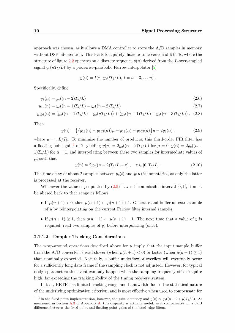
10 Signal Processing Structure
approach was chosen, as it allows a DMA controller to store the A/D samples in memory
without DSP intervention. This leads to a purely discrete-time version of BETR, where the
structure of figure 2.2 operates on a discrete sequence y(n) derived from the L-oversampled
signal yc(nTb/L) by a piecewise-parabolic Farrow interpolator [2]
y(n) = I(τ ; yc(lTb/L), l = n− 3, . . . n) .
Specifically, define
y2(n) = yc((n− 2)Tb/L) (2.6)
y12(n) = yc((n− 1)Tb/L)− yc((n− 2)Tb/L) (2.7)
y103(n) =(
yc((n− 1)Tb/L)− yc(nTb/L))
+(
yc((n− 1)Tb/L)− yc((n− 3)Tb/L))
. (2.8)
Then
y(n) =(
(
y12(n)− y103(n))
µ + y12(n) + y103(n))
µ + 2y2(n) , (2.9)
where µ = τL/Tb. To minimize the number of products, this third-order FIR filter has
a floating-point gain3 of 2, yielding y(n) = 2yc((n − 2)Tb/L) for µ = 0, y(n) = 2yc((n −1)Tb/L) for µ = 1, and interpolating between these two samples for intermediate values of
µ, such that
y(n) ≈ 2yc((n− 2)Tb/L + τ) , τ ∈ [0, Tb/L] . (2.10)
The time delay of about 2 samples between yc(t) and y(n) is immaterial, as only the latter
is processed at the receiver.
Whenever the value of µ updated by (2.5) leaves the admissible interval [0, 1[, it must
be aliased back to that range as follows:
• If µ(n + 1) < 0, then µ(n + 1)← µ(n + 1) + 1. Generate and buffer an extra sample
of y by reinterpolating on the current Farrow filter internal samples.
• If µ(n + 1) ≥ 1, then µ(n + 1) ← µ(n + 1) − 1. The next time that a value of y is
required, read two samples of yc before interpolating (once).
2.1.1.2 Doppler Tracking Considerations
The wrap-around operations described above for µ imply that the input sample buffer
from the A/D converter is read slower (when µ(n + 1) < 0) or faster (when µ(n + 1) ≥ 1)
than nominally expected. Naturally, a buffer underflow or overflow will eventually occur
for a sufficiently long data frame if the sampling clock is not adjusted. However, for typical
design parameters this event can only happen when the sampling frequency offset is quite
high, far exceeding the tracking ability of the timing recovery system.
In fact, BETR has limited tracking range and bandwidth due to the statistical nature
of the underlying optimization criterion, and is most effective when used to compensate for
3In the fixed-point implementation, however, the gain is unitary and y(n) ≈ yc((n − 2 + µ)Tb/L). Asmentioned in Section A.3 of Appendix A, this disparity is actually useful, as it compensates for a 6 dBdifference between the fixed-point and floating-point gains of the band-edge filters.

2.1 Signal Processing at the Receiver 11
small average misadjustments between the assumed and actual data rates due to Doppler
or Tx/Rx clock offset. More sophisticated Doppler compensation systems were deemed
unnecessary, as both the AUV and ASC will be stationary during acoustic transmissions.
It seems unlikely that significant mean Doppler shifts would be observed even if the AUV
and ASC where moving, since the tracking systems ensure that their relative speed is close
to zero.
2.1.2 Equalization
Residual timing jitter and intersymbol interference are removed by a (linear) fractionally-
spaced equalizer operating at 2 samples per symbol. The equalizer input vector, parameter
vector and output are denoted by y(n), c(n) and z(n) = cT (n)y(n), respectively. In a
variety of algorithms, the update recursion for c(n) may be written as
c(n + 1) = c(n) + µ(n)y∗(n)e(n) , (2.11)
where e(n) is a generalized error and µ(n) is a variable adaptation step. A fixed value for µ
is difficult to select a priori because it depends on the channel characteristics, hence all the
algorithms that were considered provide some means of dynamically adjusting the step.
The recursion (2.11) is still valid for a decision-feedback equalizer (DFE) if y(n) contains
previous symbol decisions, in addition to the input samples y(n). Although widely used
in general-purpose underwater receivers to compensate for severe ISI, decision-feedback
equalization proved to be of limited usefulness under the relatively benign acoustic chan-
nels linking the AUV and ASC. For that reason, this nonlinear structure was not built
into the software.
Based on the analysis of experimental data gathered at the test site, three adaptation
algorithms were considered to be sufficiently robust, yet simple, for inclusion in the real-
time receiver:
Soft-Constraint Satisfaction (SCS): A blind algorithm closely related to the constant-
modulus algorithm (CMA), but with enhanced convergence properties [20].
Normalized Least Mean Squares (NLMS): A reference-driven algorithm similar to
LMS, where the step depends on the norm of the equalizer input vector [10].
Adaptive step-size LMS (SLMS): Another reference-driven algorithm where both the
equalizer output MSE and the adaptation step are optimized at each iteration [10].
Some details of these algorithms will be given in the next section. Blind algorithms
were examined mainly as a convenient way of recovering from short-term channel fades
that may occur as waves induce rapid oscillations of the ASC. Although their ability
to compensate for ISI in steady-state was usually satisfactory, the initial convergence was
rather inconsistent, sometimes ranging from a few hundred symbols to several thousand in
consecutive data frames. While the clarification of such behavior is an interesting research
topic, blind equalization was considered too unreliable for the goals set forth in ASIMOV.

12 Signal Processing Structure
The SLMS algorithm is very popular in underwater equalization, as its convergence
and tracking properties approach those of recursive least-squares algorithms (RLS) with
much lower computational complexity [3]. In the ASIMOV high-speed acoustic link, how-
ever, ISI is sufficiently low for SLMS to outperform NLMS only marginally [8]. Having
somewhat lower complexity, NLMS was therefore adopted as the equalization algorithm
in the standard ASIMOV receiver.
2.1.2.1 Equalizer Order
The fractionally-space equalizer has 20 coefficients per subchannel, i.e., a total of 40 coef-
ficients. In reference-driven algorithms there are 8 anticausal coefficients per subchannel,
so that the coefficient and input vectors can be represented as
c =
[
c(0)
c(1)
]
, y(n) =
[
y(0)(n)
y(1)(n)
]
, (2.12)
where, for any i = {0, 1},
c(i) = [c(i)N1
. . . c(i)−1 c
(i)0 . . . c
(i)N2
]T , N1 = −8 , N2 = 11 , (2.13)
y(i)(n) = [y(i)(n−N1) . . . y(i)(n + 1) y(i)(n) . . . y(i)(n−N2)]T . (2.14)
The values of N1 and N2 were empirically chosen from analysis of data collected at the
test site. The initial coefficient vector is arbitrarily chosen as an impulse in subchannel 0:
c(i)k =
{
1 if i = 0, k = 0,
0 otherwise.(2.15)
Generation of the stationary “polyphase components” y(i)(n)∆= y(nL+i), i = {0, 1}, L = 2
from the (decimated) cyclostationary interpolator output y(n) involves no computational
overhead when operating in batch mode, as the latter outputs a 2-element vector with the
desired format4 [y(2n) y(2n + 1)]T = [y(0)(n) y(1)(n)]T in every symbol interval.
As usual, the training sequence is delayed by a suitable number of symbols (−N1),
so that the required anticausal input samples (with respect to the reference symbol) are
available to the equalizer. As detailed in Section 4.1, initial coarse synchronization of
data frames is achieved by transmitting a chirp preamble, whose presence can be detected
by correlation with an uncertainty of about one symbol interval. Upon convergence, the
equalizer will automatically synthetize any fine-scale delay correction that is necessary to
precisely align the reference and received sequences.
In blind equalization the notion of causal and anticausal samples is meaningless, as no
reference sequence exists. However, given coefficient and input vectors of the form (2.12)
with
c(i) = [c(i)0 . . . c
(i)N2−N1
]T , y(i)(n) = [y(i)(n) . . . y(i)(n− (N2 −N1))]T , (2.16)
4Note that here y(n) denotes the interpolated sequence decimated to L = 2 samples per symbol.

2.1 Signal Processing at the Receiver 13
the equalizer will hopefully remove the ISI and converge to an arbitrarily delayed and phase
rotated symbol a(n−d) exp jφ. The delay d depends on the initial coefficient vector; As a
rule of thumb, if the ISI is not too severe and c has a single nonzero element c(i)d , then c
(i)d
will remain the strongest coefficient upon convergence and cTy(n) ≈ a(n − d) exp jφ, as
long as d is not too close to the filter edges 0, N2−N1. By using the initialization strategy
c(i)k =
{
1 if i = 0, k = −N1,
0 otherwise,(2.17)
the equalizer output sequence in blind and reference-driven mode will have a similar delay
(usually it will differ by 2 or 3 symbols at most), which helps to accomodate both classes of
equalization algorithms more homogeneously. Note that (2.15) and (2.17) actually denote
identical coefficient vectors c, as different time indices were adopted.
2.1.2.2 Blind Algorithms
The Constant Modulus Algorithm (CMA) is a popular blind equalization algorithm due to
its simplicity and robustness [10]. The parameter vector c is adjusted so that the output
magnitude approaches a desired value R. As the CMA cost function does not depend
on the output phase, the algorithm can tolerate arbitrary carrier frequency offset and
significant phase jitter in the input signal.
The normalized CMA (NCMA) algorithm is derived using a deterministic criterion, by
minimizing ‖c(n + 1)− c(n)‖ such that the a posteriori output magnitude equals R [15].
The update recursion is very similar to conventional CMA, except that the squared norm
of the input vector is used as a normalization factor.
Soft-Constraint Satisfaction (SCS) is similar to NCMA, but a relaxation factor is
introduced when solving the deterministic constrained optimization problem [20]. This
modification reduces the number of undesirable fixed points of the adaptive algorithm for
which there is insufficient ISI cancellation. The parameters to be used in (2.11) are
µ(n) =1
‖y(n)‖2 + δn, δn = 10 , (2.18)
e(n) =z(n)
1− µ(
1− |z(n)|R
) − z(n) , µ = 0.5 , (2.19)
where δn is a small bias term that prevents numerical overflow when ‖y(n)‖2 is close
to zero and µ can, in principle, be chosen arbitrarily in the interval µ ∈]0, 1] for stable
operation.
2.1.2.3 Reference-Driven Algorithms
In all reference-driven algorithms e(n) is the difference between the (phase-synchronized)
decision made by the slicer and the equalizer output. In NLMS the adaptation step is
given by
µ(n) =µ
‖y(n)‖2 + δn, µTRN = 0.5 , µDD = 0.1 , (2.20)

14 Signal Processing Structure
where δn has the same value of (2.18), and µ ∈]0, 1] ensures stability when the channel is
time invariant. The value µ = 0.5 is used during training for fast convergence, whereas
µ = 0.1 is used in decision-directed mode to reduce constellation jitter and avoid equalizer
divergence due to feedback of wrong decisions.
In addition to (2.11), SLMS uses the following two-step recursion to update the optimal
step [10]
g(n) = dT (n)y(n) (2.21)
d(n + 1) = d(n) + y∗(n)[
e(n)− µ(n)g(n)]
(2.22)
µ(n + 1) =[
µ(n) + α Re{g(n)e∗(n)}]µ+
µ−
, (2.23)
where α is a small constant step that has little impact on performance and the bracket in
(2.23) denotes clipping of µ(n+1) to the interval [µ−, µ+]. The following numerical values
were adopted
µ(0) = 10−3 , µ− = 10−5 , µ+ = 10−2 , α = 2−15 ≈ 3× 10⁻⁵ . (2.24)
The auxiliary coefficient vector d can be interpreted as the elementwise derivative of c
with respect to the current step µ.
2.1.3 Carrier Recovery and Slicing
Carrier recovery is based on a simple and widely-used PLL algorithm [19, 13]. The in-
stantaneous phase error is given by
eθ(n) = Im{a(n)a∗(n)} , (2.25)
where a(n) = z(n) exp−jθ(n) is the equalized symbol after phase synchronization. The
corresponding slicer output a(n) = D(a(n)) is based on a memoryless nearest-neighbor
criterion denoted by the decision function D(·). The phase estimate is updated as
θ(n + 1) = θ(n) + G(z)eθ(n) , (2.26)
where G(z)eθ(n) denotes filtering of the phase error sequence by a proportional-plus-
integral (PI) loop filter
G(z) = Gp +Gi
1− βz−1, Gp = 10−1 , Gi = 1.7× 10⁻³ , β = 1− 1024−1 . (2.27)
In reference-driven algorithms, the error term to be fed back to the equalizer is e(n) =
(a(n) − a(n)) exp jθ(n), which prevents its coefficients from rotating to track common
phase variations and thereby improves the overall stability.
2.1.3.1 Low-level Slicing for 4-PSK and 8-PSK
Computing the slicer output a(n) = D(a(n)) for arbitrary constellations can be computa-
tionally intensive. To meet the real-time constraints of the receiver, specialized decision

2.1 Signal Processing at the Receiver 15
0
2
1
3
4
6
5
7
Figure 2.3: PSK constellation for low-level slicing (4-PSK restricted to real/imaginaryaxes)
functions were developed for the 4/8-PSK constellation shown in Figure 2.3. It should be
stressed that the rules described in this section pertain to the low-level slicer shown in
Figure 2.1. Higher-level mapping/unmapping functions, described in Chapter 3, may use
Trellis-coded modulation or other coding strategies5 to reduce the output bit error rate.
The slicing process resembles the metric update procedure for Trellis-coded modulation
described in Section 3.3.3. However, the numbering of constellation points in Figure 2.3
was chosen so that most of the code can be shared when slicing both 4-PSK and 8-PSK,
and thus differs slightly from Figure 3.4, which follows [23]. The ordering is immaterial
from the point of view of adapting data pump subsystems, and these specific indices were
selected simply to streamline the code.
Given an arbitrary complex point x, evaluating distances |x − yi|2 with variable yi =
4/8-PSK(i) is equivalent to computing the simpler inner product Re{xy∗i } for decision
purposes, since all points in the 4/8-PSK constellation have the same magnitude. The
following algorithm is used:
1. Four reference points of the 8-PSK constellation are chosen,
y0 = 1 , y1 = j , y2 =1√2(1 + j) , y3 =
1√2(−1 + j) .
2. The four inner products d(i) = Re{xy∗i }, i = 0, . . . 3 are calculated and stored. The
index that maximizes the magnitude, io = arg maxi |d(i)|, reveals that either yio or
−yio is the constellation point closest to x.
3. The phase error is ±Im{xy∗io}, depending on whether yio or −yio is closest to x. Since
Re{x(±y∗io)} is necessarily positive for the nearest point, the appropriate phase error
is simply obtained by computing Im{xy∗io}sgn(
Re{xy∗io})
.
4. Due to the symmetries of the constellation
d(i + 1) = Re{−jxy∗i } = Im{xy∗i } , i ∈ {0, 2} ,
5As a special case, no coding or simple differential coding may be specified, as discussed in Section3.3.2.

16 Signal Processing Structure
or, equivalently,
d(i) = Re{jxy∗i+1} = −Im{xy∗i+1} , i ∈ {0, 2} .
Then, Im{xy∗io} = (−1)iod(io ⊕ 1), where io ⊕ 1 denotes an exclusive-or operation
that complements the LSB of io, swapping the indices 0 ↔ 1 or 2 ↔ 3. Hence, the
table d(i) already constains all the required values to compute the phase error as
eθ(n) = (−1)iod(io ⊕ 1)sgn(
d(io))
. (2.28)
For 4-PSK constellations, only the first two points are considered in the previous algorithm.
The choice between both constellations is made at compile time, as documented in Section
5.3.
Interaction with high-level mapping: The following points should be carefully ob-
served when designing and selecting the mapping/unmapping functions to be used by the
transmitter and receiver.
• Obviously, the low-level slicer should be compatible with high-level coding schemes,
otherwise equalization and carrier recovery will fail, invalidating all subsequent pro-
cessing as well. To ensure this, any admissible coder must output a sequence of
complex points that conform to the raw 2D constellation6 of Figure 2.3. The same
holds for the training sequence (and marker) mapping function.
• Ideally, no bits should ever come out of the low-level slicer, its complex output
being used exclusively to adapt data-pump subsystems. However, this is strictly
not true in the ASIMOV receiver because differential decoding7 is performed on
these raw decisions to scan for start markers and the training sequence epilog, as
discussed in Section 4.2. This hard-coded technique will only work if differential
Gray-coded 4-PSK or 8-PSK is chosen as the training sequence mapping function at
the transmitter. The correspondence8 between phase jumps and data bits is shown
in Figure 3.5b,d. See Sections 4.3 and 5.3 for more details on transmitter and receiver
parameterization.
2.2 Signal Processing at the Transmitter
As one would expect, the transmitter performs few signal processing functions. Most of its
computational resources are devoted to frame formatting (Chapter 4) and coding (Chapter
6The labelling of points is irrelevant, but the shape should be respected.7In data pump functions, the choice between differential 4-PSK and 8-PSK is made at compile time.
See also Section 5.3.8For 8-PSK, the lookup table {0, 3, 1, 2, 6, 5, 7, 4} is used to map the internal indices of Figure 2.3 into
bit triplets. The same table can be used for 4-PSK by discarding the LSB of each entry.
2.2 Signal Processing at the Transmitter 17
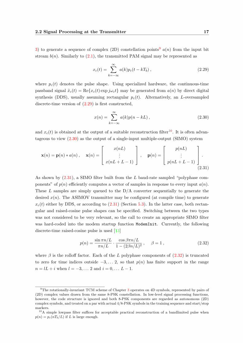
3) to generate a sequence of complex (2D) constellation points9 a(n) from the input bit
stream b(n). Similarly to (2.1), the transmitted PAM signal may be represented as
xc(t) =
∞∑
k=−∞
a(k)pc(t− kTb) , (2.29)
where pc(t) denotes the pulse shape. Using specialized hardware, the continuous-time
passband signal xc(t) = Re{xc(t) exp jωct} may be generated from a(n) by direct digital
synthesis (DDS), usually assuming rectangular pc(t). Alternatively, an L-oversampled
discrete-time version of (2.29) is first constructed,
x(n) =∞
∑
k=−∞
a(k)p(n− kL) , (2.30)
and xc(t) is obtained at the output of a suitable reconstruction filter10. It is often advan-
tageous to view (2.30) as the output of a single-input multiple-output (SIMO) system
x(n) = p(n) ∗ a(n) , x(n) =
x(nL)...
x(nL + L− 1)
, p(n) =
p(nL)...
p(nL + L− 1)
.
(2.31)
As shown by (2.31), a SIMO filter built from the L baud-rate sampled “polyphase com-
ponents” of p(n) efficiently computes a vector of samples in response to every input a(n).
These L samples are simply queued to the D/A converter sequentially to generate the
desired x(n). The ASIMOV transmitter may be configured (at compile time) to generate
xc(t) either by DDS, or according to (2.31) (Section 5.3). In the latter case, both rectan-
gular and raised-cosine pulse shapes can be specified. Switching between the two types
was not considered to be very relevant, so the call to create an appropriate SIMO filter
was hard-coded into the modem startup function ModemInit. Currently, the following
discrete-time raised-cosine pulse is used [13]
p(n) =sin πn/L
πn/L· cos βπn/L
1− (2βn/L)2, β = 1 , (2.32)
where β is the rolloff factor. Each of the L polyphase components of (2.32) is truncated
to zero for time indices outside −3, . . . 2, so that p(n) has finite support in the range
n = lL + i when l = −3, . . . 2 and i = 0, . . . L− 1.
9The rotationally-invariant TCM scheme of Chapter 3 operates on 4D symbols, represented by pairs of(2D) complex values drawn from the same 8-PSK constellation. In low-level signal processing functions,however, the code structure is ignored and both 8-PSK components are regarded as autonomous (2D)complex symbols, and treated on a par with actual 4/8-PSK symbols in the training sequence and start/stopmarkers.
10A simple lowpass filter suffices for acceptable practical reconstruction of a bandlimited pulse whenp(n) = pc(nTb/L) if L is large enough.

Chapter 3
Coding
On-site measurements indicate that noise levels in the vicinity of hydrothermal vents
can be two orders of magnitude higher than those commonly found in the open North
Atlantic ocean up to hundreds of KHz [22]. Although experiments have shown that linear
(feedforward) equalizers are able to converge under these conditions, an outer coding layer
was included to reduce the error rate in the output bit stream.
The choice of a coding strategy must take into acount the fact that bandwidth is very
tight to meet the desired user bit rate of 30 kbit/s. Additionally, M-PSK constellations
must be used due to hardware restrictions, which does not allow the available transmit
power to be exploited in the most efficient way. Without coding, it seems unreasonable to
expect acceptable error rates from constellations denser than 4-PSK, and the minimum
required symbol rate would therefore be 15 kbaud. Considering the inefficiencies that are
associated with the generation and filtering of waveforms, attaining this symbol rate would
take up virtually all the available bandwidth.
Direct coding of the bit stream using convolutional coding or other forward error cor-
recting techniques reduces the effective bandwidth available to the user. The constellation
would then have to be expanded to 8-PSK at least to compensate for the added redun-
dancy, as it is not possible to increase the symbol rate. This option was not pursued
because it was not clear whether the inevitable increase in raw symbol errors would off-
set the coding gain. A better alternative is provided by trellis-coded modulation, which
directly operates at the constellation level and introduces coding gain through temporal
diversity without increasing neither the transmitted power nor the bandwidth [21]. This is
achieved by expanding the signal set to compensate for the added redundancy but, unlike
the coding scheme mentioned above, it is done in a way that guarantees a net performance
gain relative to the uncoded case.
3.1 Coder and decoder structure
Using a rate n/n + 1 convolutional code, the TCM encoder maps blocks of n bits into
one of 2n+1 constellation points. In the ASIMOV high-speed link n = 4 is used, and
each coded symbol is formed by two pairs of complex points in an (8-PSK)×(8-PSK)
18

3.2 Interleaving 19
Input BitStream
Output BitStream
ConstellationMapping
ConvolutionalEncoder (4/5)
Interleaver
EqualizerDeinterleaverTCM Unmapper
(Viterbi)
UWAChannel
Figure 3.1: TCM coding blocks
4D constellation. When interleaving is used, the equivalent channel at the receiver after
equalization is assumed to be memoryless, and decoding of trajectories across constellation
points can be done using the Viterbi algorithm with an Euclidean distance metric based
on the known signal Trellis. Fig. 3.1 shows the general structure of the coder and decoder.
3.2 Interleaving
Convolutional interleaving/deinterleaving is used at the transmitter and receiver to sim-
plify the software implementation [18]. In this kind of structure the complex values gen-
erated at the transmitter are sequentially shifted into a bank of I parallel shift registers.
Each successive register provides one more storage unit than the preceding one. The zeroth
register provides no storage, i.e., it is a simple feedthrough connection. With each new
value the commutator switches to a new register and the corresponding value is shifted
in, while while the oldest value in that register is shifted out to the modulator. After the
(I − 1)-th register the commutator returns to the zeroth register and starts again. The
deinterleaver performs the inverse operation, and the input-output commutators for both
interleaving and deinterleaving must be synchronized.
Figure 3.2 illustrates an example of convolutional interleaving and deinterleaving for
I = 4. Figure 3.2a shows values 1 to 4 being loaded; Each ‘×’ represents an unknown
value that depends on the initial shift register internal states. Figure 3.2b shows some
of the previous values shifted within the registers and the entry of values 5 to 8 to the
interleaver input. Figure 3.2c shows values 9 to 12 entering the interleaver. At this
time the deinterleaver is now filled, but nothing useful is being fed to the decoder yet.
Finally, Figure 3.2d shows values 13 to 16 entering the interleaver, and at the output of
the deinterleaver values 1 to 4 are being passed to the decoder. The process continues in
this way until the entire sequence, in its original preinterleaved form, is presented to the
decoder.
The performance of a convolutional interleaver is very similar to that of a block inter-
leaver. An important advantage of convolutional interleaving is that the end-to-end delay
is I(I−1), and the memory required is I(I−1)/2 at both ends of the channel, which is half

20 Coding
Fromencoder
Synchronizedcommutators
Interleaver Deinterleaver
2
3
4
3
2
4
1 1
X
X
X
Todecoder
1 X
X
X
X
(a)
6
7 3
48
7
6
8
5 5
X
2
X
2
15 X
X
X
X
(b)
10
11 7
8 412
11
10
12
9 9
3
6
X
2
3
6
5 19 X
X
X
X
(c)
14
15 11
12 816
15
14
16
13 13
7
10
4
6
7
10
9 513 1
3
2
4
(d)
Figure 3.2: Illustration of convolutional interleaving and deinterleaving with depth I = 4
the corresponding requirements for block interleaving. Moreover, the processing structure
of Figure 3.2 lends itself to simple and elegant software designs. In keeping with the batch
processing philosophy introduced in Section 2.1, synchronized commutators do not exist
in the actual software implementation of the ASIMOV high-speed link. Instead, the in-
terleaver receives and delivers I-element complex vectors with the original and interleaved
values for all the shift registers, and the deinterleaver behaves analogously.
Similarly to the startup phase shown in Figure 3.2, dummy (‘×’) values should continue
to be fed to the interleaver after the end of a data block until the delay lines of the
deinterleaver have been fully emptied. During both periods, a decision was made not to
transmit these spurious values to avoid wasting bandwidth. This implies that the effective
interleaving depth is not constant across a full data block, but rather increases from 1 to
I during the startup phase, remains at I in steady state, and then decreases from I to 1
in the block epilog. This results in weaker protection against error bursts during transient

3.3 Rotationally-Invariant TCM for M-PSK Constellations 21
periods, but since they are relatively short when compared to the length of data blocks,
that limitation was deemed acceptable.
To streamline the code, the number of complex values in a data block is constrained
to be a multiple of I, so that they can fill an integer number of input/output vectors1. As
each 4D TCM symbol is represented by a pair of complex numbers, the block length is
also constrained to be a multiple of 2, so that the whole block content can be generated
from an integer number of symbols.
3.3 Rotationally-Invariant TCM for M-PSK Constellations
Frequently, rapid phase variations in the received signal induce rotations of the input
constellation that exceed the tracking rate of carrier recovery systems. This problem
is particularly relevant in the present context, where clusters of points in the expanded
constellation can have significant overlap due to noise. Depending on the phase symmetries
of the constellation, arbitrary undetectable rotations may occur before carrier lock is
regained. While a degradation in equalizer output is clearly visible during these events, the
adaptation algorithms can usually recover spontaneously and numerical divergence seldom
occurs. This problem is routinely addressed through differential coding of symbols, but
that technique is ineffective in most TCM schemes because arbitrarily-rotated trajectories
through the expanded constellation do not usually belong to the signal Trellis [21].
Some of the most popular TCM codes for 2D QAM constellations are indeed invariant
to 90o rotations, and systematic methodologies for constructing these codes have been
outlined in the technical literature. However, their generalization to more than four phase
ambiguities, as found in 8-PSK or 16-PSK, proved to be challenging. During the study of
QAM schemes it was verified that rotational invariance was easier to obtain with multidi-
mensional constellations, the reason being that some phase ambiguities may be removed
by proper partitioning of the constellation. This property carries over to multidimensional
M-PSK, and forms the basis of the rotationally-invariant TCM schemes developed in [23].
A multidimensional symbol can be sent over a two-dimensional channel (i.e., complex
single-input single-output) by sending two of its components at a time.
Specific four- and eight-dimensional schemes using Trellis encoders with up to 64 states
are described in [23] for both 8-PSK and 16-PSK. These provide coding gains ranging from
3.01 to 5.13 dB. Note that the equalizer cannot tolerate the large decoding delay of the
Viterbi algorithm, and in decision-directed mode its adaptation is based on hard decisions
provided by a memoryless slicer described in Section 2.1.3.1. This commonly-used ap-
proach essentially excludes 16-PSK TCM schemes, as the raw equalizer decisions, which
do not benefit from any coding gain, would be too unreliable and lead to frequent diver-
gence of the adaptation algorithms. Even if the equalizer does not diverge, occasional
incorrect raw decisions will lead to a transient increase in its output MSE, thereby indi-
1It is easy to convince oneself that the insertion and deletion of dummy values during startup/epilogdoes not alter this.

22 Coding
Y0
Y1
Y2
Y3
Y4
First 2-D8-PSK Index
Second 2-D8-PSK Index
4D 8-PSKConstellation
Mapping
DifferentialEncoderPSfrag replacements
b(4n)
b(4n + 1)
b(4n + 2)
b(4n + 3)
z−1z−1
000/0
1/1
0/0
1/1
1/0
0/1
0/1
1/0
10
01
11
(a) (b)
Figure 3.3: Rotationally-invariant 8-PSK TCM (a) Encoder (b) 4-State Trellis
rectly affecting the performance of the Viterbi decoder. This prevents the full predicted
TCM coding gain to be effectively realized in practical systems that incorporate adaptive
subsystems such as channel equalizers.
3.3.1 TCM Encoder
Due to complexity constraints, one of the simplest schemes with underlying 8-PSK con-
stellation was adopted for the ASIMOV high-speed link. Figure 3.3 shows the structure
of the 4-state encoder and the Trellis diagram, with an associated coding gain of 3.01 dB.
The state LSB is Y0 and the MSB is the output of the left delay block in Figure 3.3a.
Branches are labeled as input/output = Y1/Y0. Note that Y2, . . . Y4 do not enter the state
machine and have no influence on state transitions, therefore each branch in the Trellis
diagram should actually be interpreted as a super-branch formed by 8 parallel branches
for all possible values of these variables.
The encoder processes blocks of 4 consecutive bits b(4n), . . . b(4n+3), and outputs 4D
complex symbols defined by pairs of points in an 8-PSK constellation. Prior to constella-
tion mapping, bits b(4n), . . . b(4n + 2) are differentially encoded according to
{Y3 Y2 Y1}(n) =(
{Y3 Y2 Y1}(n− 1) + {b(4n + 2)b(4n + 1)b(4n)})
8, (3.1)
where (·)8 indicates that the addition is performed modulo 8. Table 3.1 shows the pairs
of 8-PSK points generated by the 4D constellation mapper of Figure 3.3. The 3-bit values
given in the table should be interpreted as indices into the 8-PSK constellation shown in
Figure 3.4.
The constellation may also be viewed as the superposition of the following 4D 2-PSK
subconstellations S0, . . . S7
S0 :(
{0, 4}, {0, 4})
S4 :(
{2, 6}, {2, 6})
S1 :(
{1, 5}, {3, 7})
S5 :(
{3, 7}, {1, 5})
S2 :(
{2, 6}, {0, 4})
S6 :(
{0, 4}, {2, 6})
S3 :(
{1, 5}, {1, 5})
S7 :(
{3, 7}, {3, 7})

3.3 Rotationally-Invariant TCM for M-PSK Constellations 23
Table 3.1: 4D 8-PSK Constellation Mapping
Y4Y3Y2Y1Y0 Pt #1 Pt #2 Si Y4Y3Y2Y1Y0 Pt #1 Pt #2 Si
0 0 0 S0(0) 16 0 4 S0(2)1 1 3 S1(0) 17 1 7 S1(2)2 2 4 S2(2) 18 2 0 S2(0)3 1 1 S3(0) 19 1 5 S3(2)4 2 2 S4(0) 20 2 6 S4(2)5 3 5 S5(2) 21 3 1 S5(0)6 4 6 S6(3) 22 4 2 S6(1)7 3 3 S7(0) 23 3 7 S7(2)8 4 4 S0(3) 24 4 0 S0(1)9 5 7 S1(3) 25 5 3 S1(1)10 6 0 S2(1) 26 6 4 S2(3)11 5 5 S3(3) 27 5 1 S3(1)12 6 6 S4(3) 28 6 2 S4(1)13 7 1 S5(1) 29 7 5 S5(3)14 0 2 S6(0) 30 0 6 S6(2)15 7 7 S7(3) 31 7 3 S7(1)
0
1
2
3
4
5
6
7
Figure 3.4: 8-PSK constellation for each half-symbol in rotationally-invariant TCM
where (Pt #1, Pt #2) indicates a pair of complex values that jointly define a 4D sym-
bol, and {·, ·} denotes the points that comprise a 2D 2-PSK subconstellation. Table 3.1
indicates the assignment of each 4D symbol to one of the Si.
3.3.1.1 16-state TCM:
In addition to the 4-state TCM scheme described above, support was added at the trans-
mitter for the 16-state coder described in Figure 6c of [23], which can provide a coding
gain of 4.13dB (see also Sections 4.3.1.1 and 5.3.1). Decoding requires a Viterbi algorithm
that is significantly more complex than the one described in Section 3.3.3. The unmapping
function was not developed, as it was considered to be too demanding for the available
hardware, both in terms of memory and computational power.

24 Coding
0
1
2
3
0
1
3
2
(a) (b)
0
1
2
3
4
5
6
7
0
1
3
2
6
7
5
4
(c) (d)
Figure 3.5: Signal constellations for non-TCM operation (a) Plain 4-PSK (b) Differentially-Gray-encoded 4-PSK (c) Plain 8-PSK (d) Differentially-Gray-encoded 8-PSK
3.3.2 Link operation with plain 4-PSK and 8-PSK
By proper choice of firmware, the ASIMOV high-speed link can also use plain 4-PSK,
optionally with differential encoding. The encoder processes 2-bit blocks to produce a
single complex point in the 4-PSK constellation depicted. As this simplified encoder is
triggered at twice the rate of the TCM encoder of Figure 3.3, the overall rate at which
input bits are read and output symbols are generated remains constant in both cases.
Figure 3.5a-b shows the signal constellations for plain and differentially-coded 4-PSK.
In the latter case, each point should be interpreted as a phase jump relative to the previ-
ously transmitted complex symbol. As usual, Gray coding is used to minimize the bit error
probability when symbol decoding errors occur between adjacent constellation points.
Fewer software changes are needed if the same constellation shape is used regardless
of whether the input to the slicer is obtained directly from the equalizer output, after
carrier synchronization, or by multiplying it with the conjugate of the previous decision in
differential mode. This explains the 45-degree rotation of Figure 3.5a relative to standard
4-QAM/4-PSK, so that it coincides with Figure 3.5b up to a permutation of points.
Depending on the options used for compiling the transmitter and receiver, plain and
differentially-encoded 8-PSK can also be specified, using the constellations shown in Fig-
ures 3.5c-d. Naturally, this will result in higher input-output bit rates if the triggering
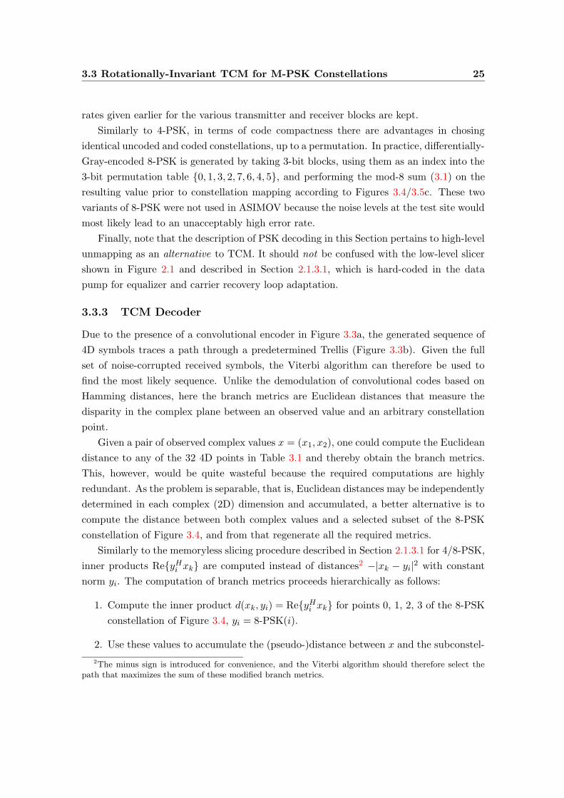
3.3 Rotationally-Invariant TCM for M-PSK Constellations 25
rates given earlier for the various transmitter and receiver blocks are kept.
Similarly to 4-PSK, in terms of code compactness there are advantages in chosing
identical uncoded and coded constellations, up to a permutation. In practice, differentially-
Gray-encoded 8-PSK is generated by taking 3-bit blocks, using them as an index into the
3-bit permutation table {0, 1, 3, 2, 7, 6, 4, 5}, and performing the mod-8 sum (3.1) on the
resulting value prior to constellation mapping according to Figures 3.4/3.5c. These two
variants of 8-PSK were not used in ASIMOV because the noise levels at the test site would
most likely lead to an unacceptably high error rate.
Finally, note that the description of PSK decoding in this Section pertains to high-level
unmapping as an alternative to TCM. It should not be confused with the low-level slicer
shown in Figure 2.1 and described in Section 2.1.3.1, which is hard-coded in the data
pump for equalizer and carrier recovery loop adaptation.
3.3.3 TCM Decoder
Due to the presence of a convolutional encoder in Figure 3.3a, the generated sequence of
4D symbols traces a path through a predetermined Trellis (Figure 3.3b). Given the full
set of noise-corrupted received symbols, the Viterbi algorithm can therefore be used to
find the most likely sequence. Unlike the demodulation of convolutional codes based on
Hamming distances, here the branch metrics are Euclidean distances that measure the
disparity in the complex plane between an observed value and an arbitrary constellation
point.
Given a pair of observed complex values x = (x1, x2), one could compute the Euclidean
distance to any of the 32 4D points in Table 3.1 and thereby obtain the branch metrics.
This, however, would be quite wasteful because the required computations are highly
redundant. As the problem is separable, that is, Euclidean distances may be independently
determined in each complex (2D) dimension and accumulated, a better alternative is to
compute the distance between both complex values and a selected subset of the 8-PSK
constellation of Figure 3.4, and from that regenerate all the required metrics.
Similarly to the memoryless slicing procedure described in Section 2.1.3.1 for 4/8-PSK,
inner products Re{yHi xk} are computed instead of distances2 −|xk − yi|2 with constant
norm yi. The computation of branch metrics proceeds hierarchically as follows:
1. Compute the inner product d(xk, yi) = Re{yHi xk} for points 0, 1, 2, 3 of the 8-PSK
constellation of Figure 3.4, yi = 8-PSK(i).
2. Use these values to accumulate the (pseudo-)distance between x and the subconstel-
2The minus sign is introduced for convenience, and the Viterbi algorithm should therefore select thepath that maximizes the sum of these modified branch metrics.

26 Coding
lations S0, . . . S7 of Table 3.1
d(x1, y0)→ S0, S6 d(x2, y0)→ S0, S2
d(x1, y1)→ S1, S3 d(x2, y1)→ S3, S5
d(x1, y2)→ S2, S4 d(x2, y2)→ S4, S6
d(x1, y3)→ S5, S7 d(x2, y3)→ S1, S1
As each 2D subconstellation of Si is 2-PSK, computing maximum pseudo-distances is
trivial. If d(xk, yi) > 0 then yi is the closest point in the 2D constellation, otherwise
the symmetrical −yi is closest and the correct metric is d(xk,−yi) = −d(xk, yi).
3. Compute the pseudo-distance between x and the 4 subconstellations
R0 = S0 ∪ S4 , R1 = S1 ∪ S5 , R2 = S2 ∪ S6 , R3 = S3 ∪ S7 .
For each Ri this simply involves comparing the metrics for Si and Si+4 and selecting
the largest.
As pointed out in [23], the value of Y1Y0 at the encoder determines the subconstellation
Ri from which a 4D point will be transmitted, and this is the mechanism that introduces
memory and provides coding gain. At this point, metrics have therefore been computed
for the super-branches of Figure 3.3b. As usual, these are now added to the path metrics,
a single survivor is selected for each state, and backtracking information is stored.
Pure maximum-likelihood sequence detection for long data packets is not really prac-
tical, as it involves a large decoding delay and requires significant storage for path back-
tracking. To circumvent these problems, the ASIMOV TCM decoder uses a simplified
Viterbi algorithm where path metrics are recursively propagated across the whole packet,
but backtracking information is only kept for a block-sliding window containing the most
recent symbols. This technique reduces the memory footprint of the algorithm at the
expense of a small penalty in output error rate. A block of (oldest) bits is extracted when
the decoding window fills up, and the latter is then shifted in time, as detailed below:
1. The upper and lower time indices of the decoding window are denoted by W+ and
W−, respectively. At the start of the decoding process they coincide with the initial
time reference, which can arbitrarily be set to 0.
2. The upper index W+ is incremented by one whenever the TCM decoder is triggered,
and therefore coincides with the most recent time reference, n.
3. When the window length W+ −W− reaches a prechosen maximum value W (i.e.,
the decoding window is full) a block of B symbols is decoded, and W− is advanced
accordingly. These are the B oldest symbols for which backtracking information is
stored.
See also the discussion regarding mapper/unmapper reset in Section 4.2.1.
Chapter 4
Data Formatting
Data sent through any communication channel must be formatted so that it can be regen-
erated by a suitably synchronized receiver. While a layered protocol stack such as the ISO
model provides several synchronization mechanisms at different layers, this report only
covers those implemented at the physical level in the ASIMOV high-speed link. The next
sections describe in detail the format and design parameters of data packets.
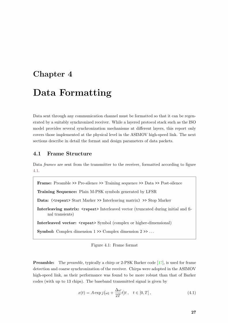
4.1 Frame Structure
Data frames are sent from the transmitter to the receiver, formatted according to figure
4.1.
Frame: Preamble >> Pre-silence >> Training sequence >> Data >> Post-silence
Training Sequence: Plain M-PSK symbols generated by LFSR
Data: (<repeat> Start Marker >> Interleaving matrix) >> Stop Marker
Interleaving matrix: <repeat> Interleaved vector (truncated during initial and fi-nal transients)
Interleaved vector: <repeat> Symbol (complex or higher-dimensional)
Symbol: Complex dimension 1 >> Complex dimension 2 >> . . .
Figure 4.1: Frame format
Preamble: The preamble, typically a chirp or 2-PSK Barker code [17], is used for frame
detection and coarse synchronization of the receiver. Chirps were adopted in the ASIMOV
high-speed link, as their performance was found to be more robust than that of Barker
codes (with up to 13 chips). The baseband transmitted signal is given by
x(t) = A exp j(
ωl +∆ω
2Tt)
t , t ∈ [0, T [ , (4.1)
27

28 Data Formatting
where ωl/2π = −7.5 kHz, ∆ω/2π = 15 kHz, and T ≈ 10.7 ms (or 640 sample intervals at
a sampling frequency of 60 kHz). By differentiating the phase of (4.1), the instantaneous
frequency of this signal is seen to increase linearly from −7.5 kHz to 7.5 kHz relative to
the carrier frequency, thus covering the full signal bandwidth of 15 kHz. The amplitude A
coincides with that of the main data waveform in the frame. Detection of chirp preambles
is based on a mixed energy and correlation criterion as follows.
• After baseband conversion and AGC, the squared magnitudes of the received samples
are applied to an AR filter with a single pole at z = 0.95. Its (real) output provides
a short-term estimate of the received signal power.
• Concurrently, the real and imaginary parts are quantized to 1 bit (0/1) and cross-
correlated with a similarly quantized local replica of the desired chirp signal. This
process is carried out efficiently by the same functions that are used for marker and
training sequence scanning in the frame.
Suitable thresholds are defined for these variables, and a preamble is detected when both
are exceeded.
Pre- and Post-Silence: The purpose of these signal gaps is to wait for echos to die-out
after signal transmission, thus improving the robustness of an ensuing detection process
(preamble or training sequence scanning). At a sampling frequency of 60 kHz, the pre-
and post-silence periods last for 300 and 100 sampling intervals, respectively.
Training Sequence: Similarly to the V.34 protocol, binary training data is obtained by
applying a sequence of 1’s to a linear-feedback shift register (LFSR, or scrambler) whose
initial state is initialized with 0’s. The constellation mapping function that converts these
bits to complex symbols need not be the same one used for data. This allows, e.g., plain
4-QAM to be used during training and more complex signal mapping (differential, TCM)
during actual data transmission.
The scrambler which is used for other purposes besides training, operates as follows.
Given an input bit at time n, u(n), the scrambled bit is computed as
s(n) = u(n)⊕ s(n− 1)⊕ s(n− 15) , (4.2)
where ⊕ denotes modulo-2 addition (xor). Whenever necessary, scrambling is inverted by
u(n) = s(n)⊕ s(n− 1)⊕ s(n− 15) . (4.3)
The feedback connection pattern ensures that a maximal-length sequence (or M-sequence)
is generated, with period 215− 1.
4.1.1 Frame data
As depicted in Figure 4.1, the data portion of a frame is obtained by concatenating start
markers and interleaving matrices, followed by a single stop marker.

4.1 Frame Structure 29
4.1.1.1 Markers and data scrambling
Start and stop markers are generated by the same scrambler used for training, by forcing
suitable initial states defined in Section 4.3. These seeds are chosen such that the cross
correlation between markers and the training sequence is weak for typical lengths. An
equivalent scrambler (i.e., same order and tap coefficients) is applied to the input data to
break long sequences of identical bits that might have a negative impact on symbol/carrier
recovery and equalization. The initial state of this scrambler is reset to 0 at the start of
each interleaving matrix.
4.1.1.2 Interleaving matrices
An interleaving matrix simply designates the concatenation of several interleaver output
vectors, i.e., sets of complex values sequentially read from the delay lines of Figure 3.2 for
each time instant.
To limit the propagation of errors when large interleaving depths are used, the delay
line contents are discarded at the start of each matrix, making them self-contained. As
discussed in Section 3.2, transient effects thus occur at the beginning and end of each
matrix, as the delay lines are being filled and then emptied. Specifically, suppose that a
depth-I convolutional interleaver should generate a total of V I complex values per matrix.
Then the transmitter should process V + I − 1 vectors per matrix as follows:
• Let n ≥ 1 denote the time index, and v(n) the corresponding interleaver output
vector. For n = 1, . . . I − 1 only the first n elements of v(n) contain symbols that
should be transmitted. The remaining ones are invalid and should be discarded.
• For n = I, . . . V the full vector v(n) should be transmitted.
• For n > V the interleaver should be fed with arbitrary (nondata) symbols. Only the
last V + I − n components of v(n) contain valid symbols to be transmitted.
As expected, the total number of transmitted complex values is
2
I−1∑
n=1
n + (V − I + 1)I = 2(I − 1)I
2+ (V − I + 1)I = V I . (4.4)
The receiver processes the V + I − 1 vectors v(n) according to:
• For each n, the transmitted components of v(n) are demodulated and input to the
convolutional deinterleaver. Arbitrary values are used for the discarded components.
• As depicted in Figure 3.2, all deinterleaver outputs are invalid while n < I. For
n = I, . . . V + I − 1 full vectors are available at the deinterleaver output, yielding a
total of V I complex values.

30 Data Formatting
4.1.1.3 Symbol mapping
As discussed in Section 3.3.1, symbols are 4D (complex pairs) when rotationally-invariant
TCM is used, and 2D (complex scalars) in plain M-PSK. To simplify the software im-
plementation, if is convenient for the interleaver/deinterleaver to always operate on plain
complex numbers regardless of the underlying constellation dimensionality. Moreover, its
input and output vectors should contain an integral number of symbols. For that reason,
its depth is not directly specified, but rather set by the product of two configuration pa-
rameters: the number of constellation complex dimensions and the interleaving depth per
constellation complex dimension.
Unmapping Delay When demodulating TCM symbols there is an initial latency while
filling the Trellis window, as described in Section 3.3.3. Although bits are extracted from
the Trellis on a block basis, the unmapping function stores these values in an internal
bit buffer so that they can be conveyed to the caller one symbol interval at a time. The
unmapping buffer’s smoothing action ensures that, after the initial latency, a suitable
number of bits1 is available from the unmapping function as long as it is invoked once
per symbol interval. This issue does not arise in plain M-PSK, where unmapping is
memoryless.
Due to the unmapping delay, the trailing (deinterleaved) symbols of each matrix are
only retrieved at the start of the next one. Because interleaving matrix lengths are chosen
such that the Trellis window fills up at the start of all matrices other than the first one2,
it would seem easy to design transmit/receive functions that could handle this delay with
little code overhead. However, a design choice was taken to handle all matrices identically,
and in a self-contained way. The transmitter thus generates dummy bits while feeding the
mapper to generate the final W symbols in a matrix, where W denotes the unmapping
delay, so that a full3 Trellis window supports the detection of any true data bit. These
final bits are decoded but discarded at the start of the next frame, which introduces some
inefficiency in the communication process. This was deemed acceptable for the operating
parameters of interest.
As an alternative to having dummy trailer bits while keeping interleaving matrices
strictly isolated, one could envision feeding the unmapping function with arbitrary symbols
(ideally, as many as the unmapping delay) after processing all the interleaving vectors to
extract the remaining data bits. This strategy was not adopted, as it would lead to
unreliable decisions and corrupt the Trellis, which should be reused undisturbed when
demodulating the next interleaving matrix4.
1log2 of the number of points in the constellation (cardinality).2See the discussion on mapper/unmapper reset in Section 4.2.1.3This is only approximately true when the block decoding strategy of Section 3.3.3 is used.4Arguably, this violates the principle of self-containment in interleaving matrices. See the discussion
on mapper/unmapper reset in Section 4.2.1 for justification of this procedure.

4.1 Frame Structure 31
4.1.1.4 Character and bit stuffing
At the transmitter, input bytes are stored in a character buffer, typically filled by a serial
port, and moved to a bit buffer as needed. The bit buffer provides the actual data for
frame generation, and is filled on demand either by the character buffer or by internal bit
stuffing functions. Stuffing amounts to insertion of one or more 8-bit default character
codes (0xC1) into that buffer, to satisfy a read request from the frame generating function.
The following algorithm is used:
1. If the buffer contains enough bits to satisfy the request, return the appropriate
quantity.
2. If not, tentatively read one more characters from the character buffer. If none is
available, insert a default code and return to step 1.
3. Otherwise, check if (a stuffed version of) that character still fits on the current
interleaving matrix. If not, insert a default code and return to step 1.
4. Read the character, stuff it as appropriate, insert it into the bit buffer, and return
to step 1.
Stuffing of an input character c is required when it is similar to the default code. In
that case, it is replaced by an expansion code and additional information for unstuffing,
according to the following rules:
• The expansion code equals the default code with MSB set to 0.
• If c(MSB-1)...c(0) equals the corresponding bits in the default and expansion
codes, then stuffing is required.
• In that case, c is augmented by appending a 0 between c(MSB) and c(MSB-1). The
resulting bit pattern equals the expansion code, concatenated by the original c(MSB).
A similar two-buffer architecture is used at the receiver, where the character buffer is
typically associated with an output serial port. Bits extracted from the incoming frame
are stored in a bit buffer, and moved to a character buffer whenever enough data are
available to regenerate one output byte, as described below:
1. Insert the bits from the frame scanning function into the bit buffer.
2. While the bit buffer contains at least a plain character’s worth of bits, examine the
pattern. If it is a default code, remove it from the buffer and discard it.
3. If not, check whether it is an expansion code. If so, but not enough bits are available,
return.
4. Read the required number of bits, unstuff if appropriate, write the result into the
character buffer, and go back to step 2.

32 Data Formatting
The bit buffers at the transmitter and receiver are emptied at the start of each interleaving
matrix, making them self-contained. This effectively resynchronizes character boundaries
following each start marker, which is a desirable feature in practice. Depending on the type
of data being sent, it may be appropriate to use the contents of the current interleaving
matrix, even if character boundary loss in the previous one led to extensive data corruption.
Packetization and Data/Command Modes: If specified at compile time, more com-
plex bit and character management mechanisms may be used. In that operating mode, the
bit stream is broken into a sequence of packets. Each packet starts with a synchronization
flag, followed by the bits corresponding to an integer number of characters5. Bit stuffing
is used to ensure that the start flag occurs only at the beginning of a packet. Should
the receive modem loose synchronization of character boundaries, it may recover once the
next start flag is detected. This may provide finer-grained synchronization than the one
already available from start markers between interleaving matrices, but involves a loss in
data throughput.
The maximum number of bits per packet, including the flag, is configurable. If the
maximum packet size cannot contain an integer number of characters, including stuffing
bits, then the packet will be (slightly) abbreviated. If not enough input data exist to fill
the current packet, or the remaining number of data bits in the interleaving matrix cannot
hold a full packet, then the packet will be truncated. When the input character buffer is
empty (or the packet size is so small that it cannot hold one character plus the start flag),
then packet start flags (’empty’ packets) will be generated until the required number of
symbols per matrix is attained.
Transmitter: All characters received through the serial port are stored in an input
character buffer, which should be large enough to absorb all processing delays that are
inherent in the operation of the modem. The transmitter may operate in data mode or
command mode, and the character buffer is processed differently in both cases. In data
mode, characters are removed from the character buffer and placed in a transmit bit buffer
as they are needed to fill each packet. The bit buffer may also be filled by packet start
flags and stuffing bits. Since it is filled ’on demand’, the bit buffer need not be very large,
but must be efficiently accessed.
In command mode the input characters are interpreted as configuration commands
and parameters. Toggling between the two modes is achieved by transmitting a special
sequence of characters known as a break flag (typically +++) that may be redefined as
appropriate. Input characters are processed sequentially, so that all commands must be
interpreted before starting to transmit data frames and vice-versa. This means that data
characters before and after a sequence of commands are completely isolated, and will never
be included in the same frame. This may induce some inefficiency by allowing the last
5The number of bits per character is configurable, so ASCII or binary data may be handled simply andefficiently.

4.2 Layered Processing at the Receiver 33
frame before a command sequence to be padded with empty packets instead of useful
data. However, this limitation is deemed acceptable because (i) command sequences are
not frequently used, and (ii) modem management procedures are thus greatly simplified.
Receiver: At this level, receiver operations mirror those of the transmitter. The
incoming bit stream is scanned for packet start flags, destuffed, and sent to a bit buffer if
the flag is not detected. The bit buffer size need only be slightly larger than the number of
bits that make up a character. As soon as an appropriate number of bits is available from
the bit buffer, a character is removed from it and stored in the output character buffer.
To maintain synchronization of character boundaries, the bit buffer is reset when a packet
start flag is detected. The output character buffer should be large enough to smooth out
the latencies involved in sending data through the serial port.
Similarly to the transmitter, an input character buffer accepts commands and data,
toggling between both modes when break flags are detected. When in data mode the
receiver simply discards the contents of this buffer and resumes processing of incoming
frames.
4.2 Layered Processing at the Receiver
The transmitter software generates frames according to the model of Figure 4.1 by a
hierarchy of functions with no side effects, which hopefully makes the code relatively
easy to understand and maintain. A similar software structure would be desirable for
the receiver, but some compromise must be made between code modularity and the need
to provide global resynchronization mechanisms upon detection of start markers in the
incoming symbol stream. This section discusses some of the issues involved.
Preamble Scanning: The receiver continuously tries to detect and decode incoming
frames. It may be convenient to interrupt it, e.g., when operating in command/data mode
and new configuration parameters are received in the input character buffer. For that
purpose, a pointer is passed to the preamble scanning function, so that it may be aborted
by externally writing an appropriate (nonzero) value to this memory location. This feature
would also be useful when implementing timeouts.
Data Pump Reset: Low-level signal processing functions (data pump) are reset before
processing the training/data portion of a frame. Although the initial parameters for these
systems are somewhat arbitrary, resetting them to a known default state limits the worst
case behavior. This is relevant, e.g., in integrators and equalizers, which may take a long
time to reconverge following an abrupt change in the properties of their input processes.
Because frames may be arbitrarily spaced, there is no a priori reason to suppose that the
data pump parameters should be preserved.

34 Data Formatting
Training Sequence: Handling of training sequences is straightforward in reference-
driven equalization. If the receiver is coarsely synchronized by the frame preamble, so that
in each symbol interval the equalizer input vector contains most of the energy pertaining
to the specified reference symbol, then the training process will automatically provide fine
synchronization. In other words, the coefficient vector will evolve so that at time n the
equalizer output z(n) approximately equals the reference symbol a(n), and the overall
discrete equivalent channel response approaches an impulse.
The situation is different when blind equalization is used because then, as discussed in
Section 2.1.2.1, an unknown delay and phase rotation may exist upon convergence such
that z(n) ≈ a(n − d) exp jφ. To cancel the delay d the receiver must scan for a known
fragment of the training sequence and align itself accordingly. This is accomplished as
follows:
1. The final 256 bits6 of the training sequence are generated and stored in the main
data pump module.
2. Equalizer output symbols are differentially decoded by the low-level slicer of Figure
2.1 and stored in a bit buffer when approaching the end of the training sequence
(specifically, when the nominal time left equals the temporal span of the local training
replica plus 20 symbol intervals). Naturally, this requires the use of differential
coding when mapping the training sequence. To attain the necessary efficiency, only
4-PSK and 8-PSK constellations can be specified (at compile time). For more details,
see Sections 2.1.3.1 and 3.3.2.
3. When the differentially decoded bit buffer is full, pattern scanning begins. If the
number of bit matches exceeds a threshold (90% of the buffer length), a flag is
raised to signal training lock. Subsequent calls to the training function perform no
function while this flag is set, effectively freezing the input waveform until the local
time reference reaches the end of the training sequence. A sufficiently large buffer
must exist to absorb the input samples that are acquired while the data pump is
frozen.
4. If lock was not attained until the nominal end of the training sequence, pattern
scanning is performed up to an additional 20 symbol intervals. No valid reference is
available during this period, but that poses no problem because such scanning will
only be required when blind equalization is used.
Residual Phase Synchronization: When training lock is attained the most recent
input to the low-level slicer is saved by the data pump. Due to carrier synchronization the
constellation should be aligned with Figure 2.3 at this point of the processing chain, up
to a residual rotation ambiguity of nπ/4 (8-PSK) or nπ/2 (4-PSK) in blind equalization
6The stored bit pattern length depends on the width of unsigned long on the target processor, whichis assumed here to be 32 bits.

4.2 Layered Processing at the Receiver 35
mode. Moreover, the last reference symbol is saved by the high-level management function
invoked during training. These two complex values will subsequently be compared to
eliminate the residual rotation before proceeding to the next frame decoding stage. This
operation is essential if a non-differential mapping mode is used for interleaving matrix
transmittal. With differential modes, it ensures that the differential decoder state is set
appropriately, so that the first symbol is correctly decoded.
Marker Scanning: Marker sequences are handled similarly to training sequences, but
no phase resynchronization is attempted upon successful detection. This could lead to re-
ceiver breakdown when non-differential mapping modes are used if carrier synchronization
is lost in the middle of a frame. This potential problem was considered to be relatively
unimportant in the context of the present work, which focuses on differential mappings.
The following procedure is used for marker scanning:
1. When approaching the end of an interleaving matrix, low-level differential decoding
and storage of received symbols is initiated (See Section 2.1.3.1).
2. When the interleaving matrix has been fully processed, the receiver enters a ded-
icated marker detection phase where differential decoding and storage continue.
Events are timed so that the scanning buffer is filled with a full marker’s worth
of bits 4 symbol (2D 4/8-PSK) intervals before its nominal endpoint. Marker scan-
ning then begins.
3. Scanning continues until up to 4 symbol intervals after the marker nominal endpoint.
This function promptly terminates upon marker detection, returning a suitable code
(start/stop/none). A failure counter is decremented if no start marker is found in a
time window of ±4 symbols, otherwise the counter is reset to a configurable value
(currently 1) that defines the maximum allowed number of consecutive detection
misses. If the failure counter reaches zero, then it is assumed that the receiver is
hopelessly lost and frame decoding is aborted. If not the next interleaving matrix is
processed.
4. As mentioned in Section 4.1.1.4, character boundaries are aligned at the start of each
interleaving matrix by emptying the output bit buffer. To limit the propagation of
errors, the data scrambler (Section 4.1.1.1) is reset to a known state.
4.2.1 Mapper/Unmapper Reset:
To ensure that interleaving matrices are self-contained, the unmapping function should
be reset7, in addition to the scrambler and bit buffer. This is problematic when TCM is
used because resetting the Trellis path metrics reduces the error protection at the start of
a new (deinterleaved) matrix. Additionally, resetting the state of the built-in differential
7Naturally, resetting of the bit buffer, scrambler, and unmapping function should be mirrored by equiv-alent operations at the transmitter.

36 Data Formatting
encoder/decoder in rotationally-invariant TCM will cause a decoding error at the receiver
if the received signal constellation is rotated relative to the one assumed at transmission.
To tackle this problem, two distinct reset levels were considered. A hard reset is
performed at the start of the first interleaving matrix, setting the Trellis state, path
metrics, differential encoder/decoder state and decoding window to default values. A soft
reset is performed at the start of all remaining matrices, which performs no operation at
the transmitter and forces the Trellis window to a default state at the receiver. This will
also implicitly resynchronize the buffer of (differentially encoded) symbols.
The lengths of both the trellis window and interleaving matrices are selected so that
state forcing is redundant if there is no loss in synchronization, that is, the forced state
should equal the one that arises after normally processing a matrix. Specifically, the
Trellis window should fill up when the first symbol of a (deinterleaved) matrix is sent to
the unmapper.
Let M be the total number of symbols per interleaving matrix8, W the maximum
Trellis window size and B the length of the block that is decoded from a full Trellis
window (see Section 3.3.3). Note that W exceeds the unmapping delay by 1.
First matrix: After an initial lattency of W −1 symbols to fill the Trellis window, blocks
of data are decoded at intervals of B symbols (the bits are stored in a buffer and
gradually released over B calls to the unmapping function). According to the “almost
full” default Trellis condition assumed in (soft) resets, the next time for extracting
a block would be one symbol after the end of the matrix (which lasts from time 0 to
M − 1), hence
W − 1 + kB = M , k integer. (4.5)
Remaining matrices: Blocks of data are decoded at intervals of B symbols with no
initial latency. As before, the next time for extracting a block would be one symbol
after the end of the matrix,
lB = M , l integer. (4.6)
Equating the two expressions it becomes apparent that W − 1 (unmapping delay) must
be a multiple of B. Given W and B, the interleaving depth and number of interleaving
blocks are selected so that M satisfies the first expression.
4.3 Transmitter and Receiver Configuration
This section describes the main variables that are used to parameterize the transmitter
and receiver, and provides sample configurations. The text organization parallels the
software implementation, where these variables are grouped into structs declared in
8For 4D TCM symbols M = V I/2, where the right-hand term is derived from (4.4).

4.3 Transmitter and Receiver Configuration 37
several modules. More details on the software architecture and configuration options are
given in Chapter 5.
4.3.1 Frame Parameters (modem.c)
The FramePar structure defines the overall frame parameters. It contains the following
fields:
BaudRate: Number of 2D constellation points transmitted per second in the data portion
of a frame9.
Oversamp: Number of samples generated or collected per 2D constellation point. The
(baseband) sampling rate is BaudRate*Oversamp.
Constel: Structure holding the signal constellation parameters for training, markers and
data.
TrnBitsPerSymbol: Number of bits per (2D) constellation point in training se-
quences and start/stop markers.
TrnMap: Pointer to training sequence and marker mapping function. For compati-
bility with the low-level slicer of Section 2.1.3.1, this should be differentially-
Gray-coded 4-PSK or 8-PSK.
BitsPerSymbol: Number of bits per constellation point in data (inside interleaving
matrices).
CDimPerSymbol: Number of complex dimensions per data symbol, i.e., number of
complex values that make up a symbol.
Map: Pointer to data mapping function.
ResetMap: Pointer to the resetting function of the data mapper.
UnMap: Pointer to data unmapping function.
ResetUnMap: Pointer to the resetting function of the data unmapper.
UnMapDelay: Unmapper latency, i.e., number of symbols submitted to the unmap-
ping function before the first decoded bit becomes available.
• UnMapDelay = 0 in memoryless and plain differential mappings.
• UnMapDelay is 1 unit less than the Trellis window depth when TCM is used.
UnMapBlk: Number of symbols to decode and remove when the Trellis window fills
up. UnMapDelay should be a multiple of it.
PreWait: Number of sampling periods between the end of the preamble and the start of
the training sequence.
9This parameter is something of a misnomer when 4D TCM is used, as symbols are formed by pairs ofcomplex numbers and the real baud rate, i.e., the number of transmitted symbols per second, is actuallyhalf this value.

38 Data Formatting
TrainSeqLen: Length of training sequence, i.e., number of 2D differential 4/8-PSK con-
stellation points.
MarkLen: Length of start/stop markers, i.e., number of 2D differential 4/8-PSK constel-
lation points.
StartMarkSeed, StopMarkSeed: Initial value to be loaded into the linear-feedback shift
register that generates start/stop markers (Section 4.1.1.1). The same structure is
used for training sequence generation, with 0 initial configuration.
IlCDimDepth: Interleaver depth per complex dimension in data symbols. The interleaving
depth is thus IlCDimDepth*CDimPerSymbol. This awkward format ensures that an
integral number of (possibly multidimensional) data symbols fits in each interleaver
input/output vector (Section 4.1.1.2).
IlBlk: (Equivalent) number of full vectors per interleaving matrix. As shown by (4.4),
transient effects while filling and emptying a convolutional interleaver/deinterleaver
are such that the total number of complex values in a matrix is a multiple of the
interleaving depth.
MtxPerFrame: Number of interleaving matrices per frame.
PostWait: Minimum number of sampling periods after the frame epilog (stop marker)
before a new frame may begin.
4.3.1.1 Mapping Functions
Pointers in the Constel structure can be set according to the following list of available
constellation mapping functions. Inclusion of the actual source code for these functions
is controlled by several compile-time definitions listed in Section 5.3.1. The practical
procedure is demonstrated in the makefiles of Section 5.4. For each modulation type,
mapping, unmapping and, if applicable, reset function names are indicated. As memoryless
mappings have no internal state variables, their reset pointers should be set to NoReset,
a dummy function that performs no operation.
Plain 2-PSK: PSK2Map, PSK2UnMap.
Differentially-Gray-coded 2-PSK: DPSK2Map, DPSK2UnMap, DPSK2ResetMap,
DPSK2ResetUnMap.
Plain 4-PSK: QAM4Map, QAM4UnMap.
Differentially-Gray-coded 4-PSK: DQAM4Map, DQAM4UnMap, DQAM4ResetMap,
DQAM4ResetUnMap.

4.3 Transmitter and Receiver Configuration 39
Double differentially-Gray-coded 4-PSK: DQAM4x2Map, DQAM4x2UnMap,
DQAM4x2ResetMap, DQAM4x2ResetUnMap. This mode is the same as differential 4-
PSK, but two complex constellation points are processed simultaneously. It was
included in the project to test the handling of 4D symbols (used in rotationally-
invariant TCM) by upper layers of the transmitter and receiver.
Plain 8-PSK: PSK8Map, PSK8UnMap.
Differentially-Gray-coded 8-PSK: DPSK8Map, DPSK8UnMap, DPSK8ResetMap,
DPSK8ResetUnMap.
Rotationally-invariant 4-state TCM: TCM4Map, TCM4UnMap, TCM4ResetMap,
TCM4ResetUnMap.
Rotationally-invariant 16-state TCM: TCM16Map, TCM16ResetMap. As described in
Section 3.3.1.1, support for this TCM mode only exists in transmit mode due to
limitations in the available computational power.
4.3.1.2 Differential Encoder/Decoder State:
All differentially-Gray-coded PSK modes share the same state variable to simplify saving
and restoring it when a start marker is generated. Saving/restoring ensures that trans-
mission of marker symbols is transparent as far as data symbols are concerned, even if
the same differential PSK mapping function is used for both10. This operation ensures
consistency with TCM modes, which use an internal differential coder that is not affected
by transmission of marker symbols using differential 4/8-PSK.
No similar save/restore is needed at the receiver because marker and training symbols
are demodulated by a low-level slicer (Section 2.1.3.1), and never sent to the high-level
unmapper that extracts data bits. Still, a single state variable is used for all differential
PSK modes at the receiver as well.
4.3.2 Generic Data Pump Parameters (dpump.c)
Currently, the top level data pump module is configured simply by setting the behavior
of the low-level slicer (Section 2.1.3.1) via two #defines.
PSK8SYNC: If TRUE (1), the full constellation of Figure 2.3 is used when formulating symbol
decisions to be fed back to the carrier recovery loop and equalizer. If FALSE (0) only
the 4 points in the real and imaginary axes are considered. Note that 8-PSK mode
should be selected when operating in TCM, even if marker and training symbols are
4-PSK. This may be considered somewhat suboptimal as it increases the probability
of wrong decisions in 4-PSK symbols, thus leading to enhanced adaptation noise. On
10The same applies to training symbols, which are in fact generated by the same function used formarkers. The fact that the saved differential encoder state before training is constant because all variablesare reset at the start of a frame is not relevant.

40 Data Formatting
the other hand, recall that marker and training epilog detection mechanisms were
introduced (Section 4.2) because there is some uncertainty in the temporal alignment
of frames, so deciding a priori which symbols should be decoded as 4-PSK or 8-PSK
is problematic11.
DPSK8MARK: If TRUE (1), differential decoding for training/marker scanning assumes the
8-PSK constellation of Figure 2.3. If FALSE (0), 4-PSK decoding is based on the
restriction of Figure 2.3 to the real and imaginary axes.
Similarly to constellation mapping functions, it would be possible to declare a function
pointer referencing any of the available equalization algorithms. This, however, was not
done, and two specific function calls were built into the source code of dpump.c. Specif-
ically, these are located in functions DpTrain and DpDecode, which manage all signal
processing blocks during training and data/marker reception, respectively. On hindsight,
and bearing in mind the likelihood that this code will be used as part of a testbed for
evaluating equalization algorithms, the minor loss in performance associated with an in-
direct function call would be more than offset by the convenience of selecting the desired
algorithm simply by filling in a variable.
4.3.3 Timing Recovery Parameters (betr.c)
The TrPar structure defines several band-edge timing recovery parameters. The numerical
values used in Chapter 2 are given between square brackets.
Fh, Fl: Upper and lower band-edge filter parameters. For each one, the following vari-
ables are defined:
NDelays [= 3]: Filter order (number of elements in state vector).
DelayLine: Filter state vector
FbCoeffs, FfCoeffs: Feedback and feedforward coefficients. The values are given
in Tables A.2 and A.3.
ScaleFb: Scaling factor for FbCoeffs[0], to be used in fixed-point arithmetic (see
Table A.3).
FLoop: Loop filter parameters.
Kp [= 5e-3], Ki: Proportional and integral gains in (2.5). The integral gain is
currently unused.
4.3.4 Carrier Recovery Parameters (psksync.c)
The CrPar structure defines carrier recovery parameters.
11Admittedly, there is virtually no ambiguity throughout most of the training sequence, but switchingfrom 4-PSK to 8-PSK slicing near the epilog would complicate the code.

4.3 Transmitter and Receiver Configuration 41
FLoop: Loop filter parameters.
SPe: Sum of phase errors at the output of the leaky integrator in (2.27).
Kp [= 1e-1], Ki [= 1.7e-3]: Proportional and integral gains in (2.27).
4.3.5 Equalization Parameters (equaliz.c)
The equalization module is configured by the following #defines. Typical values, some of
which were mentioned in Section 2.1.2, are given between square brackets.
MIDCOEF [1]: Initial equalizer coefficient for delay 0 in channel12 0. All the remaining co-
efficients are set to 0. This parameter is mainly relevant in blind equalization, where
a null coefficient vector is an undesirable equilibrium point of most cost functions.
EQNORMEPS [10]: Small positive constant that is added to the equalizer input vector norm
to prevent overflow. Used in SCS and NLMS.
SCSREF [1]: Desired equalizer output modulus for the SCS algorithm.
SCSSTEP [0.5]: SCS step size.
SLMSARLG [-15]: log2 of SLMS step adaptation rate.
SLMSSTHI [1e-2]: SLMS Maximum step.
SLMSSTLO [1e-5]: SLMS Minimum step.
SLMSSTINI [1e-3]: SLMS Initial step.
NLMSSTHI [0.5]: NLMS step size during training.
NLMSSTLO [0.1]: NLMS step size in decision-directed mode.
EQCHAN [2]: Number of equalizer input channels. The decimation factor after timing re-
covery (see Section 2.1) is calculated so that the resulting oversampling rate matches
this parameter. For proper operation, it should divide the input oversampling factor
(FramePar.Oversamp).
EQLENPERCHAN [20]: Number of equalizer coefficients per input channel. The requirement
of equal orders on all channels is not a serious restriction when the equalizer is linear
and operates on a single sensor. It would be more problematic in a decision-feedback
equalizer or when operating with multiple sensors.
EQFILL [8]: Number of anti-causal samples per channel. As usual, the equalizer reference
is delayed to emulate the existence of noncausal samples. This is achieved in a
transparent way by reading from the input sample buffer (via the timing recovery
12As discussed in Section 2.1.2, the number of channels, or polyphase components, in a fractionally-spaced equalizer equals the oversampling rate when a single physical sensor is used.

42 Data Formatting
loop) during startup of the data pump, i.e., whenever a new frame has been detected.
The procedure is harmless, though pointless, when blind equalization is used.
Provision was made for a compile-time switch (EQDESIGN, see Section 5.3) which would
enable the calculation of causal/anti-causal equalizer orders as appropriate for a given
scenario. This option was not implemented, so the equalizer order is currently hard-coded
based on EQCHAN, EQLENPERCHAN and EQFILL.
4.3.6 Sample Configuration: 4-PSK
The parameters provided below configure the transmitter and receiver for operation in
basic differentially-Gray-coded 4-PSK mode with no interleaving.
/* In modem.c */
FramePar = {15000, /* BaudRate */
4, /* Oversamp */
{ /* Constel */
2, /* TrnBitsPerSymbol */
2, /* BitsPerSymbol */
1, /* CDimPerSymbol */
DQAM4Map, /* TrnMap */
DQAM4Map, /* Map */
DQAM4ResetMap,/* ResetMap */
DQAM4UnMap, /* UnMap */
DQAM4ResetUnMap, /* ResetUnMap */
0, /* UnMapDelay */
0 /* UnMapBlk */
},
300, /* PreWait */
1000, /* TrainSeqLen */
16, /* MarkLen */
0xc07f, /* StartMarkSeed */
0x2459, /* StopMarkSeed */
1, /* IlCDimDepth */
480, /* IlBlk */
77, /* MtxPerFrame */
400}; /* PostWait */
/* In dpump.c */
#define PSK8SYNC FALSE
#define DPSK8MARK FALSE

4.3 Transmitter and Receiver Configuration 43
Notes:
1. The sampling rate is 60 kHz (BaudRate*Oversamp).
2. Differential 4-PSK is used to generate 1000 (TrainSeqLen) training symbols (TrnMap),
for a total of 2000 bits (TrainSeqLen*TrnBitsPerSymbol).
3. By design, the same mapping function is used to generate marker symbols. Each
marker is 16 symbols long (MarkLen), or 32 bits. According to (4.2), the bit pattern
of start markers is obtained by initializing a 16-bit linear-feedback shift register
(scrambler) with the lower 15 bits of StartMarkSeed
s(n− 15) . . . s(n− 1) = 100000001111111b = 0xc07f & 0x7fff ,
and then applying to it a sequence of 32 1’s. The stop marker bit pattern is generated
similarly based on StopMarkSeed. Both seeds are chosen so that markers have
low correlation with each other and the training sequence epilog. Note that the
marker and training sequence lengths are far smaller than the repetition period of
the maximal length sequence output by the scrambler (215 − 1 = 32767 bits).
4. Differential 4-PSK is also used for data (Map, UnMap). As discussed in Section
4.3.1.2, even in this case transmission of marker symbols is transparent as far as
data symbols are concerned. Each symbol is formed by a single complex constellation
point, therefore the number of complex dimensions per symbol (CDimPerSymbol) is
1.
5. It is important to ensure that the number of bits per symbol (TrnBitsPerSymbol,
BitsPerSymbol) matches the cardinality of the associated constellations. In 4-PSK
the number of bits should be log2 4 = 2.
6. No window is needed for decoding differential 4-PSK, therefore UnMapDelay and
UnMapBlk are set to 0 (see also Sections 3.3.3 and 4.2.1).
7. In the absence of coding, there is no advantage in interleaving symbols. The inter-
leaving depth is thus set to 1 (IlCDimDepth*CDimPerSymbol).
8. Interleaving matrices are 480 vectors long (IlBlk). For depth 1 each vector is formed
by a single complex value, yielding 480 4-PSK symbols per matrix.
9. There are 77 matrices per frame (MtxPerFrame), totaling 36960 data symbols or
73920 bits. The overall number of symbols, including training and start/stop markers
is 1000 + 77(16 + 480) + 16 = 39208, or 78416 bits, lasting for about 5.2 s.
10. The low-level slicer (Section 2.1.3.1) is configured to assume a 4-PSK constellation
both when providing symbol decisions for carrier recovery/equalization (PSK8SYNC)
and when decoding bits for training/marker scanning (DPSK8MARK).

44 Data Formatting
4.3.7 Sample Configuration: 4-State TCM
A more elaborate configuration is now provided, using interleaved 4-state rotationally-
invariant TCM in data matrices. The training sequence and start/stop markers are gen-
erated as in the previous section. Sample makefiles are given in Section 5.4 to actually
build the executables.
/* In modem.c */
FramePar = {15000, /* BaudRate */
4, /* Oversamp */
{ /* Constel */
2, /* TrnBitsPerSymbol */
4, /* BitsPerSymbol */
2, /* CDimPerSymbol */
DQAM4Map, /* TrnMap */
TCM4Map, /* Map */
TCM4ResetMap, /* ResetMap */
TCM4UnMap, /* UnMap */
TCM4ResetUnMap, /* ResetUnMap */
24, /* UnMapDelay */
6 /* UnMapBlk */
},
300, /* PreWait */
1000, /* TrainSeqLen */
16, /* MarkLen */
0xc07f, /* StartMarkSeed */
0x2459, /* StopMarkSeed */
16, /* IlCDimDepth */
15, /* IlBlk */
118, /* MtxPerFrame */
400}; /* PostWait */
/* In dpump.c */
#define PSK8SYNC TRUE
#define DPSK8MARK FALSE
Notes:
1. Training data and markers are generated as in Section 4.3.6.
2. 4D TCM symbols are formed by pairs of complex 8-PSK constellation points, hence
CDimPerSymbol is 2. These are generated by taking blocks of 4 bits (BitsPerSymbol),
using them to generate an additional redundant bit, and indexing a 32-point 4D con-
stellation with the resulting 5 element vector (Figure 3.3).

4.3 Transmitter and Receiver Configuration 45
3. The mapping function for TCM (Map) is independent from the one used for training
and markers. This ensures transparency in marker generation (Section 4.3.1.2).
4. The Viterbi decoder uses a Trellis window spanning 25 TCM symbols (UnMapDelay+1).
Filling it at the start of the first interleaving matrix causes a latency of 24 symbol
periods. As shown below, a judicious choice of matrix lengths (Section 4.2.1), and
insertion of dummy padding symbols (Section 4.1.1.3), ensures that all remaining
matrices experience the same latency as well.
5. When the Trellis window fills up, the 6 oldest TCM symbols are decoded (UnMapBlk).
This parameter divides UnMapDelay, as required by (4.5)–(4.6) with
B = UnMapBlk*CDimPerSymbol = 12 ,
W − 1 = UnMapDelay*CDimPerSymbol = 48 .
6. The interleaving depth is 32 (IlCDimDepth*CDimPerSymbol). This is the length of
complex vectors handled by the convolutional interleaver and deinterleaver.
7. Each matrix comprises enough (2D) constellation points to fill 15 (IlBlk) full inter-
leaving vectors, i.e., 480 complex values. This satisfies (4.5) with M = 480, W = 49,
B = 12, k = 36, and (4.6) with l = 40.
8. Satisfying (4.5)–(4.6) ensures constant initial latency in interleaving matrices, even
in the absence of soft resets (Section 4.2.1). Out of the 960 bits in each frame
(IlBlk*IlCDimDepth*BitsPerSymbol), the last 96 (UnMapDelay*BitsPerSymbol)
are not data, but dummy bits that are needed to support this operating mode.
9. There are 118 matrices per frame (MtxPerFrame), totaling 113280 bits (101952 data,
11328 dummy). The overall number of bits, including training (2000) and start/stop
markers (32 each) is 2000 + 118(32 + 960) + 32 = 119088, or 59544 complex values.
Each frame therefore lasts about 4 s.
10. The low-level slicer (Section 2.1.3.1) is configured to assume an 8-PSK constellation
when providing symbol decisions for carrier recovery/equalization (PSK8SYNC), and
4-PSK when decoding bits for training/marker scanning (DPSK8MARK).

Chapter 5
Software Organization
The transmitter and receiver software architecture was originally designed with the goal
of allowing most of the operating parameters described in Section 4.3 to be changed on-
the-fly by configuration commands conveyed through an input character buffer1. While
this would be a desirable feature in a dedicated testbed for underwater communications, it
requires some effort to ensure that both channel endpoints share the same set of parameters
at all times. This could be achieved, e.g., by including in every transmitted frame all
the operating parameters, or engaging in a negotiation process following any parameter
changes (at the transmitter) to resynchronize the receiver2. Any of these options would
involve some reduction in net bandwidth and an increase in code complexity.
Bearing in mind the limitations in manpower and available hardware, in the course of
this work reconfigurability was eventually dropped in favor of higher net data rates and a
lower memory footprint. Still, the software retained most of its original flexible design, so
that the truncated functionality can be easily added in the future.
The choice between fixed- or floating-point arithmetic is one of the most important de-
sign issues, which is usually dictated by the target processor. Although the primary target
for the ASIMOV project was a 16 bit fixed-point DSP (Texas Instruments TMS320C54x),
an effort was made to allow easy porting of the code to other processors. As described in
Section 5.2, the current design enables the specification of fixed- or floating-point arith-
metic at compile time with virtually no performance penalty. Moreover, for improved
performance one can select native compiler support for complex numbers (GNU C com-
piler).
5.1 Software Modules
This section lists all the higher-level software modules (.c and .h files), grouped by func-
tion, that are needed for building PC executables. The DSP version includes an optimized
assembly language implementation of some numeric functions, as well as specialized low-
1Typically, this buffer would be fed by a serial port.2The availability of a bidirectional medium-speed link might enable parameter changes at the receiver
to be conveyed to the transmitter.
46

5.1 Software Modules 47
level modules, not described here, that initialize the target board and interact with its
peripherals.
5.1.1 Modem Management and Testing
debug: Replacement of preamble scanning and sample I/O functions for offline modem
testing.
dptest: Simple control module for offline testing of data-pump functions (bare-bones
replacement of modem and sample/bit/character buffer management).
iosamp: Interface with A/D and D/A converters and sample queue management. File
I/O when in debug mode (incomplete).
modem: High-level modem management functions. Generation and scanning of frame
preambles, training sequences, markers and interleaving matrices (see Figure 4.1).
In debug mode, the frame parameters are read from framepar.
5.1.2 Bit/Character Buffer Management
bitmng: Modem-specific bit buffer management. Bit and character stuffing, optional pro-
cessing of bitstreams for packet generation and scanning.
buffer: General-purpose bit and character buffer management.
charmng: Processing of character streams for command/data mode switching (incom-
plete).
cmd: Processing of modem configuration commands (incomplete).
tokens: Token searching in text strings for command processing.
5.1.3 Frame Preambles
barker: Generation and scanning of Barker code frame preambles (incomplete).
chirp: Generation and scanning of chirp frame preambles.
5.1.4 Data Pump
betr: Band-edge timing recovery. In debug mode, its parameters are read from trpar.
dpump: Main data-pump module. Management of symbol/carrier recovery, equalization,
and marker/training sequence scanning. In debug mode, its parameters are read
from dppar.
equaliz: Equalization. In debug mode, its parameters are read from eqpar.
farrow: Farrow interpolation used in timing recovery.

48 Software Organization
psksync: Carrier recovery and low-level slicing (see Section 2.1.3.1). In debug mode, its
parameters are read from crpar.
5.1.4.1 Filtering
filter: General-purpose filtering and coefficient adaptation functions, and prototype
pulse generation. Supported filter structures include single-input single-output IIR
(direct form II with and without transposition), multiple-input single-output FIR,
and single-input multiple-output FIR. SISO IIR are used as band-edge filters in tim-
ing recovery (Appendix A), MISO FIR as fractionally-spaced equalizers, and SIMO
FIR as pulse shapers at the transmitter.
pulsemng: Modem-specific management of pulse shaping filters.
5.1.5 Mapping/Unmapping
map: Bit and symbol transformations. Includes functions for bit scrambling, convolu-
tional interleaving of complex vectors, and simple bit-to-symbol mapping (plain and
differential 2/4/8-PSK).
tcm8psk: Bit-to-symbol mapping using trellis-coded-modulation in an expanded 8-PSK
constellation. Includes a 4-state coder and Viterbi decoder, as well as a 16-state
coder.
5.1.6 Numeric Functions
costab: 256-element cosine lookup table in fixed-point format (16 bits, Q15). It is used
to generate exp jφ factors used in carrier recovery and low-level slicing, equalizer
adaptation, and chirp generation.
fixptdef: Definition of fixed-point numeric precision throughout the receiver signal pro-
cessing chain.
numeric: Real and complex arithmetic functions in fixed and floating point. For maxi-
mum efficiency, these may be replaced by assembly-language versions optimized for
a desired processor.
nzeros: Lookup table containing the number of zeros in all 8-bit integers. Used for
scrambling and bit pattern scanning (markers or training sequence epilog).
5.2 Numeric Implementation
Careful consideration must be given to the fixed-point representation of values across
the signal processing chain, as the numerical ranges involved vary significantly. With
only 16 bits available in the target processor, one could hardly expect to accomodate all
values using a single fixed-point format. Instead, values are appropriately scaled as they

5.2 Numeric Implementation 49
propagate through the receiver, so that at any given point the numerical representation
ensures suitable accuracy. This is typically achieved by supplying a scaling argument to
binary operators, so that conversion to the output format is done as part of the final
shifting operation whenever products are involved. The computational overhead of fixed-
point conversion is therefore minimal (in fact, almost negligible), while making optimal
use of special DSP registers that can hold extended-precision results after multiplication.
Choice of Fixed-Point Precision: Naturally, the floating-point implementation sup-
plies a reference for choosing fixed-point formats. As a first step, a software “probe” is
inserted at any desired location in the code to log floating-point values to file. These
values are subsequently imported into Matlab to determine a sufficiently tight fixed-point
format, with suitable safety margins to prevent overflow. With 16 bits available, the Qi
fixed-point format places the decimal point to the right of bit Di, i = 0, . . . 15, and uses
two’s complement notation to represent values. This approximately corresponds to i bits
for the fractional part of a real number, 1 for its sign, and the remaining 16 − i − 1 bits
for the magnitude of its integer part.
Once the appropriate format for any variable of interest is selected, it is defined as a
constant in fixptdef. In the code, scaling factors for numerical operations are then written
as a function of the precisions of its source and destination variables. As the resulting
expression is fully evaluated during compiler preprocessing, this approach involves no
performance penalty. As an example, suppose that the chosen precision for variables x, y,
z is Qi, Qj, Qk, respectively, and z = xy is to be calculated. Then, the 32-bit integer xy
should be (arithmetically) right shifted by i + j − k bits to yield z in the desired format.
Rounding: Rounding to the nearest integer requires adding 1 to the bit located imme-
diately to the right of the target LSB in the extended-precision result prior to shifting.
This is important, e.g., in the leaky integrators used inside carrier and timing recovery
loops, to avoid excessive buildup of rounding errors.
Verification: The fixed-point accuracy at any point can be ascertained by logging nu-
meric values to disk in fixed- and floating-point implementations, importing both time
series into Matlab, and comparing their evolution. Specifically, if a floating-point value x
is represented in fixed-point Qi by xi, then x ≈ 2−ixi. Significant deviations between the
two values might be caused by coarse quantization (i should be larger), or a buildup of
numerical errors in previous processing stages.
In retrospect, being able to compare fixed- and floating-point implementations of es-
sentially the same code simply by recompiling the program turned out to be a powerful
means of accelerating the development cycle. It should be kept in mind that algorithmic,
numerical and coding aspects become somewhat coupled when designing a fixed-point im-
plementation; tuning the fixed-point format frequently suffices to obtain suitable accuracy
at a given point of the signal processing chain, but sometimes major changes to the al-

50 Software Organization
gorithms are needed to get more stable numerical behavior. This was the case, e.g., with
the relatively sharp band-edge filters described in Section A.3. The final direct form II
transposed structure was chosen to avoid having internal variables with large numerical
ranges, which led to unacceptable rounding errors in other filter architectures.
5.3 Compile-time Definitions
To avoid building unnecessarily large executables, extensive use is made of conditional
compilation using #ifdef directives. This section lists several variables which should be
defined at compile time to include various parts of the code. The procedure is demon-
strated in Section 5.4. Configuration parameters for specific modules are described in
Section 4.3.
TXMODEM: Include code for transmission.
RXMODEM: Include code for reception.
FIXPT: Generate fixed-point code only (integer arithmetic).
GNUCPLX: Use native complex data types of GNU GCC compiler (fixed- or floating point).
SCANDESIGN: Compute required values for marker scanning from frame parameters, oth-
erwise use hard-coded values.
BREAKTST: Include code to scan for command/data escape sequences in the characters
that are locally sent to the modem.
PACKETTST: Generate and scan for packet start flags in the decoded bit stream.
PULSE: Generate samples of the baseband waveform by filtering the symbol sequence with
a PAM pulse (implemented as a raised-cosine SIMO filter, as described in Section
2.2. The oversampling factor is set by Oversamp, defined in Section 4.3). Other-
wise, directly output the real and imaginary parts of symbols, effectively setting the
transmit oversampling factor to 1.
DDS: Write (& read for debugging purposes) complex symbols as indices in an M-PSK
constellation, according to the format of ORCA’s modulator hardware (see Section
2.2). This option should only be used when PULSE is not defined.
DSP: Include specific code for DSP implementation.
DEBUG: Include debugging code, mainly sample read/write to/from files.
MSS: Monitor dynamic memory allocation and use.
Other secondary definitions, listed below, control code generation for various subsystems.
As these are less likely to be changed, they are defined in header files to limit the number
of required command-line options.
5.3 Compile-time Definitions 51
BETRDESIGN (betr.h): Compute upper and lower band-edge filters for timing recovery
(not implemented), otherwise use hard-coded values.
EQDESIGN (equaliz.h): Compute equalizer order (not implemented), otherwise use fixed-
size coefficient and input vectors.
EQNORM (equaliz.h): Recursively compute the equalizer input vector norm by exploit-
ing its temporal shift structure (Mandatory. Nonrecursive computation not imple-
mented).
NLMS (equaliz.h): Include code for normalized LMS (nonblind) equalization.
SCS (equaliz.h): Include code for soft-constraint satisfaction blind equalization.
SLMS (equaliz.h): Include code for adaptive step-size LMS (nonblind) equalization.
MISOFIR (filter.h): Include code for MISO FIR filtering.
SIMOFIR (filter.h): Include code for SIMO FIR filtering.
SISOII (filter.h): Include code for SISO type II filtering.
SISOTII (filter.h): Include code for SISO type II transposed filtering.
SISOFIR (filter.h): Include code for SISO FIR filtering.
5.3.1 Mapping Functions
Below is a set of compile-time variables that control the inclusion of source code for the
various mapping functions listed in Section 4.3.1.1.
DPSK2: Include differential 2-PSK mapping functions (plain 2-PSK always present).
DQAM4: Include differential 4-QAM mapping functions (plain 4-QAM always present).
DQAM4x2: [Used for debugging purposes] Include 4D pseudo-differential 4-QAM mapping
functions. Automatically incorporates DQAM4.
PSK8: Include plain 8-PSK mapping functions.
DPSK8: Include differential 8-PSK mapping functions. Automatically incorporates PSK8.
TCM4: Include rotationally-invariant 4-state 4D 8-PSK Trellis Coded Modulation (TCM)
mapping functions.
TCM16: Include rotationally-invariant 16-state 4D 8-PSK TCM mapping functions3.
3Only available at the transmitter. See also Sections 3.3.1.1 and 4.3.1.1.

52 Software Organization
5.4 Sample Makefiles
These makefiles (for GNU make) demonstrate how to build PC executables for the trans-
mitter and receiver whose parameters are specified in Section 4.3.7.
5.4.1 Transmitter
CFLAGS = -DTXMODEM -DDEBUG -DDQAM4 -DTCM4\
-DPULSE -DSIMOFIR -DM_PI=3.14159265358979323846
TXOBJ = bitmng.o buffer.o charmng.o chirp.o\
costab.o debug.o filter.o iosamp.o map.o\
modem.o numeric.o nzeros.o pulsemng.o\
tcm8psk.o
txmodem: TXOBJ
modem.o: framepar.c
5.4.2 Receiver
CFLAGS = -DRXMODEM -DDEBUG -DDQAM4 -DTCM4 -DSCANDESIGN\
-DFIXPT -DM_PI=3.14159265358979323846
RXOBJ = betr.o bitmng.o buffer.o charmng\
chirp.o costab.o debug.o dpump.o\
equaliz.o farrow.o filter.o iosamp.o\
map.o modem.o numeric.o nzeros.o\
psksync.o tcm8psk.o
rxmodem: RXOBJ
modem.o: framepar.c
dpump.o: dppar.c
betr.o: trpar.c
equaliz.o: eqpar.c
psksync.o: crpar.c

Appendix A
Band-Edge Timing Recovery
Band-edge timing recovery (BETR) was originally proposed by Godard in [4], and further
developed by Jablon [11]. This appendix briefly describes the basics of that method. The
continuous-time received baseband PAM signal in the absence of noise is given by
yc(t) =∑
k
a(k)hc(t− kTb) ,
as in (2.1) for ηc(t) = 0. Assuming that the symbol sequence a(k) is uncorrelated, with
zero mean and variance σ2a, the instantaneous power
E{
|yc(t)|2}
= σ2a
∞∑
k=−∞
|hc(t− kTb)|2 (A.1)
is periodic, with period Tb (i.e., yc(t) is a cyclostationary signal). A Fourier series expansion
of the form
E{
|yc(t)|2}
=σ2
a
Tb
∞∑
k=−∞
ckej 2kπ
Tbt
(A.2)
yields
ck =
∫ Tb
0
∞∑
k=−∞
|hc(t− kTb)|2e−j 2kπTb
tdt =
∫ ∞
−∞|hc(t− kTb)|2e−j 2kπ
Tbtdt
=1
2π
∫ ∞
−∞Hc(ω)H∗
c
(
ω − 2kπ
Tb
)
dω .
(A.3)
Baseband PAM pulse spectra are typically bandlimited to |ω| < π/Tb, and the same holds
for the multipath-distorted replica Hc(ω) (Figure A.1). Usually, the excess bandwidth1 of
these pulses is smaller than 100%, so that all ck are zero when k /∈ {−1, 0, 1}. As c−1 = c∗1,
(A.2) is seen to represent a nonzero-mean sine wave; The goal of BETR is to determine the
instant t ∈ [0, Tb) where its maximum is reached, while reducing the jitter that arises from
the random nature of the symbol sequence a(k). As seen from (A.3), the coefficients c−1
and c1 only depend on the upper and lower portions of Hc(ω), labeled Hh(ω) and Hl(ω)
1The excess bandwidth of Hc(ω) is defined as the frequency range above ω = π/Tb where |Hc(ω)| 6= 0,divided by the Nyquist bandwidth π/Tb.
53

54 Band-Edge Timing Recovery
PSfrag replacements
− πTb
πTb
Hl(ω)
Hh(ω)
Hc(ω)
ω
Figure A.1: PAM pulse spectrum
PSfrag replacementsc0
Tb
σ2aE
{
|yc(t)|2}
Re{
c1ej 2π
Tbt}
Im{
c1ej 2π
Tbt}
topt0 Tb
Figure A.2: BETR cost function
in figure A.1. As the mean value 〈E{
|yc(t)|2}
〉 = σ2ac0/Tb does not affect the location of
the maximum, (A.2) can be replaced by the alternative cost function
E{
|yc(t)|2}
− σ2a
Tb
c0 = Re{2σ2
a
Tb
c1ej 2π
Tbt}
. (A.4)
Noting that c1ej 2π
Tbt
has constant magnitude, the maximum of (A.4) is reached when
Im{
c1ej 2π
Tbt}
= 0. That is precisely the criterion used in BETR to adapt a PLL that tracks
the optimal sampling instant (Figure A.2). The imaginary part of c1ej 2π
Tbt
also vanishes
at the minimum of the cost function, but that is an unstable point of the adaptation
algorithm. Any jitter due to a(k) will move the operating point away from it, ensuring
convergence to the desired timing estimate.
Consider the complex PAM signals yh(t) and yl(t), obtained by ideal bandpass filtering
of yc(t) so that their pulse shapes become Hh(ω) and Hl(ω), respectively (see Figure A.1).
These filters are denoted by Bh(ω) and Bl(ω) in Figure 2.2. Then E{
yh(t)y∗l (t)}
is Tb-
periodic, and can be expanded in a Fourier series as
E{
yh(t)y∗l (t)}
= σ2a
∞∑
k=−∞
hh(t− kTb)h∗l (t− kTb) =
σ2a
Tb
∞∑
k=−∞
ckej 2kπ
Tbt, (A.5)

A.1 Band-Edge Filter Design 55
a(0) 1 b(0) 0.00170386383818a(1) −2.65757729365461 b(1) 0.00511159151455a(2) 2.46253341289720 b(2) 0.00511159151455a(3) −0.79132520853712 b(3) 0.00170386383818
Table A.1: Lowpass prototype for band-edge filters
where
ck =1
2π
∫ ∞
−∞Hh(ω)H∗
l
(
ω − 2kπ
Tb
)
dω . (A.6)
It is clear from (A.5)–(A.6) that only c1 may be nonzero, coinciding with the respective
Fourier coefficient of E{
|yc(t)|2}
. By replacing E{·} with a time average of Tb-spaced
samples and choosing t ∈ [0, Tb) to cancel the imaginary part of (A.5), the original cost
function (A.2) is maximized. As the bandwidth of yh(t) and yl(t) is much smaller than
that of yc(t), this approach ensures better immunity against noise and jitter than would
be possible if timing estimates were directly calculated from |yc(t)|2.
A.1 Band-Edge Filter Design
In practice, yh(n) and yl(n) are generated by rational bandpass filters Fh(ω) = Ah(ω)/Bh(ω)
and Fl(ω) = Al(ω)/Bl(ω), obtained from a common lowpass prototype
F (ω) =A(z)
B(z)
∣
∣
∣
∣
z=ejω
,A(z)
B(z)=
b0 + b1z−1 + . . . + bpz
−p
1 + a1z−1 + . . . + aqz−q. (A.7)
The transformation is given by
Bh(ω)
Ah(ω)=
B(ω − ωh)
A(ω − ωh),
Bh(z)
Ah(z)=
b0 + (b1ejωh)z−1 + . . . + (bpe
jωhp)z−p
1(a1ejωh)z−1 + . . . + (aqejωhq)z−q, (A.8)
Bl(ω)
Al(ω)=
B(ω − ωl)
A(ω − ωl),
Bl(z)
Al(z)=
b0 + (b1ejωl)z−1 + . . . + (bpe
jωlp)z−p
1 + (a1ejωl)z−1 + . . . + (aqejωlq)z−q, (A.9)
where ωh and ωl are the upper and lower band-edge frequencies, respectively. In the
baseband case of figure A.1 ωh = 2π/(2Tb), ωl = −2π/(2Tb), but note that BETR can also
be performed on passband waveforms. The filter order should be kept small when designing
the lowpass prototype, so that real-time filtering does not become to computationally
complex. This rules out Butterworth filters. However, the roots of A(z) and B(z) should
not be too close to the unit circle, as this leads to internal variables in the filtering
structure that have large dynamic ranges and cannot be accurately represented in fixed-
point arithmetic. This rules out elliptic filters. Finally, Chebyshev type I filters (equiripple
in the passband, monotonic in the stopband) were chosen as a good compromise. Section
A.2 provides Matlab code for computing the band-edge filters. For the given specifications,
a prototype of order p = q = 3 was obtained with coefficients given in table A.1. Figure
A.3 shows its magnitude and phase response.

56 Band-Edge Timing Recovery
0 0.1 0.2 0.3 0.4 0.5 0.6 0.7 0.8 0.9 1−250
−200
−150
−100
−50
0
Normalized Angular Frequency (×π rads/sample)
Mag
nitu
de (
dB)
0 0.1 0.2 0.3 0.4 0.5 0.6 0.7 0.8 0.9 1−300
−250
−200
−150
−100
−50
0
Normalized Angular Frequency (×π rads/sample)
Pha
se (
degr
ees)
0 0.1 0.2 0.3 0.4 0.5 0.6 0.7 0.8 0.9 1−50
−45
−40
−35
−30
−25
−20
−15
−10
−5
0
Normalized Angular Frequency (xπ rads/sample)
Mag
nitu
de (
dB)
(a) (b)
Figure A.3: Lowpass prototype for band-edge filters (a) Magnitude/phase frequency re-sponse (b) Detail of passband
A.2 Matlab Code for Generating Band-Edge Filters
%
% Compute band-edge filter responses for band-edge timing recovery (BETR)
%
fc = 0; % Carrier frequency
Tb = 1/15000; % Symbol interval
b = 1/Tb/2; % Excess bandwidth (roloff/(2*Tb))
L = 4; % Samples/symbol (oversampling factor)
%---------------------------------------------------------------------------
% Parameters for band-edge filters
%---------------------------------------------------------------------------
ws = 2*pi/(Tb/L); % Sampling frequency
% Continuous-time upper and lower
% band-edge center frequencies
wh = 2*pi*(fc+1/(2*Tb));
wl = 2*pi*(fc-1/(2*Tb));
% Convert to discrete frequency 0..2pi
wh_be = 2*pi/ws*(wh - fix(wh/ws));
wl_be = 2*pi/ws*(wl - fix(wl/ws));
% Ideal (continuous-time) bandwidth of
% band-edge filters around upper and
% lower band-edge frequencies
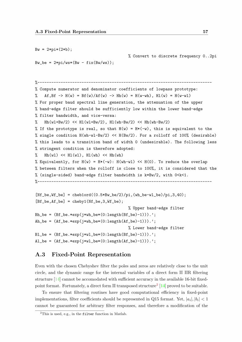
A.3 Fixed-Point Representation 57
Bw = 2*pi*(2*b);
% Convert to discrete frequency 0..2pi
Bw_be = 2*pi/ws*(Bw - fix(Bw/ws));
%---------------------------------------------------------------------------
% Compute numerator and denominator coefficients of lowpass prototype:
% Af,Bf -> H(w) = Bf(w)/Af(w) -> Hh(w) = H(w-wh), Hl(w) = H(w-wl)
% For proper baud spectral line generation, the attenuation of the upper
% band-edge filter should be sufficiently low within the lower band-edge
% filter bandwidth, and vice-versa:
% Hh(wl+Bw/2) << Hl(wl+Bw/2), Hl(wh-Bw/2) << Hh(wh-Bw/2)
% If the prototype is real, so that H(w) = H*(-w), this is equivalent to the
% single condition H(wh-wl-Bw/2) << H(Bw/2). For a rolloff of 100% (desirable)
% this leads to a transition band of width 0 (undesirable). The following less
% stringent condition is therefore adopted:
% Hh(wl) << Hl(wl), Hl(wh) << Hh(wh)
% Equivalently, for H(w) = H*(-w): H(wh-wl) << H(0). To reduce the overlap
% between filters when the rolloff is close to 100%, it is considered that the
% (single-sided) band-edge filter bandwidth is k*Bw/2, with 0<k<1.
%---------------------------------------------------------------------------
[Nf_be,Wf_be] = cheb1ord((0.5*Bw_be/2)/pi,(wh_be-wl_be)/pi,3,40);
[Bf_be,Af_be] = cheby1(Nf_be,3,Wf_be);
% Upper band-edge filter
Bh_be = (Bf_be.*exp(j*wh_be*(0:length(Bf_be)-1))).’;
Ah_be = (Af_be.*exp(j*wh_be*(0:length(Af_be)-1))).’;
% Lower band-edge filter
Bl_be = (Bf_be.*exp(j*wl_be*(0:length(Bf_be)-1))).’;
Al_be = (Af_be.*exp(j*wl_be*(0:length(Af_be)-1))).’;
A.3 Fixed-Point Representation
Even with the chosen Chebyshev filter the poles and zeros are relatively close to the unit
circle, and the dynamic range for the internal variables of a direct form II IIR filtering
structure [14] cannot be accomodated with sufficient accuracy in the available 16-bit fixed-
point format. Fortunately, a direct form II transposed structure2 [14] proved to be suitable.
To ensure that filtering routines have good computational efficiency in fixed-point
implementations, filter coefficients should be represented in Q15 format. Yet, |ai|, |bi| < 1
cannot be guaranteed for arbitrary filter responses, and therefore a modification of the
2This is used, e.g., in the filter function in Matlab.

58 Band-Edge Timing Recovery
PSfrag replacements −a1
−a2
b0
b1
b2
y(n)x(n)
z−1
z−1
PSfrag replacements
G
−a1
−a2
b0
b1
b2
y(n)x(n)
z−1
z−1
(a) (b)
PSfrag replacements−a1
−a2
b0
b1
b2
x(n)y(n)
z−1
z−1
PSfrag replacements
G
−a1
−a2
b0
b1
b2
x(n)y(n)
z−1
z−1
(c) (d)
Figure A.4: Standard and modified direct form II filtering structures (a) Standard (b)Modified (c) Standard transposed (d) Modified transposed
filter structures, shown in Figure A.4, was introduced to account for this possibility. With
the additional arbitrary coefficent G the filter transfer function becomes
F (z) =G
[
b0 + b1z−1 + . . . + bpz
−p]
1 + G[
a1z−1 + . . . + aqz−q] . (A.10)
By choosing G with sufficiently large magnitude, all other coefficients in the numerator
and denominator of (A.10) can be represented in Q15 format. Section A.4 provides Matlab
code for generating both the fixed and floating-point filter parameters from the transfer
function polynomials. They are listed in Tables A.2 and A.3 for the parameters assumed
in Section A.2. Note that the coefficients of Table A.3 induce a DC gain of 2 relative
to the floating-point frequency response. As explained in Section A.4, this stems from
the fact that the numerator coefficients of Table A.2 were scaled by 2 prior to conversion
to Q15 format in order to improve the numerical accuracy. As it turns out, this is con-
venient in practice because the floating-point implementation of the Farrow interpolator
has gain 2, whereas the corresponding gain in fixed point is 1. The cascade of this inter-

A.4 Matlab Code for Computing Filter Parameters 59
Upper Band-Edge Filter
a(0) 2.65757729365461 b(0) 0.00064113425497a(1) 0.70710678118655 · (−1− j) b(1) 0.00136005113801 · (1 + j)a(2) 0.92660838831551 · j b(2) 0.00192340276490 · ja(3) 0.21054944381730 · (1− j) b(3) 0.00045335037934 · (−1 + j)
Lower Band-Edge Filter
a(0) 2.65757729365461 b(0) 0.00064113425497a(1) 0.70710678118655 · (−1 + j) b(1) 0.00136005113801 · (1− j)a(2) 0.92660838831551 · −j b(2) 0.00192340276490 · −ja(3) 0.21054944381730 · (1 + j) b(3) 0.00045335037934 · (−1− j)
Table A.2: Floating-point band-edge filter coefficients (DC gain 1)
Upper Band-Edge Filter
a(0) 21771 (Q13) b(0) 42a(1) 23170 · (−1− j) b(1) 89 · (1 + j)a(2) 30363 · j b(2) 126 · ja(3) 6899 · (1− j) b(3) 30 · (−1 + j)
Lower Band-Edge Filter
a(0) 21771 (Q13) b(0) 42a(1) 23170 · (−1 + j) b(1) 89 · (1− j)a(2) 30363 · −j b(2) 126 · −ja(3) 6899 · (1 + j) b(3) 30 · (−1− j)
Table A.3: Fixed-point band-edge filter coefficients (DC gain 2)
polator with each band-edge filter therefore has the same overall gain in both numerical
implementations, which can simplify the specification of loop filter parameters for timing
recovery.
A.4 Matlab Code for Computing Filter Parameters
%
% Compute fixed and floating-point parameters for band-edge filters
%
% Note: Numerator and denominator polynomials for the desired rational
% transfer functions are assumed to have been previously calculated
%
%---------------------------------------------------------------------------
% Find the greatest magnitude among filter coefficients. For simplicity, a
% single value is determined for both filters. This is harmless in the
% baseband case (and of little relevance otherwise), as the symmetry in the
% frequency domain ensures that the same result would have been obtained
% with two independent scaling factors.
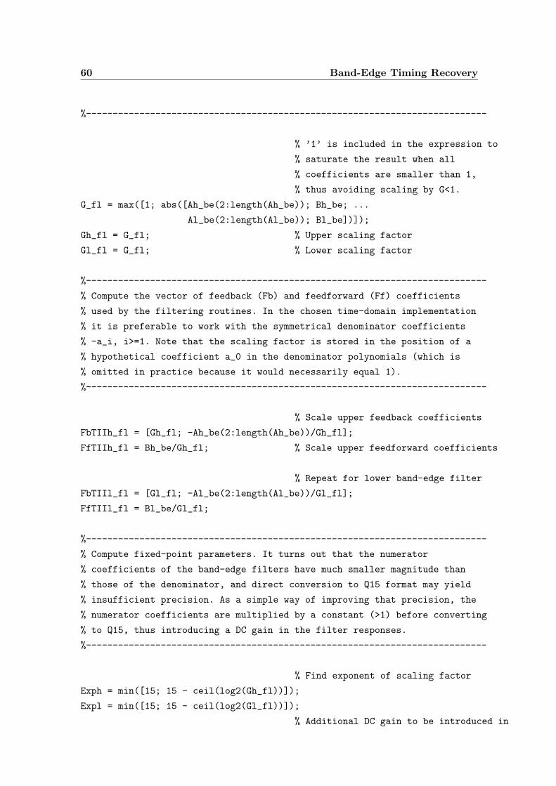
60 Band-Edge Timing Recovery
%---------------------------------------------------------------------------
% ’1’ is included in the expression to
% saturate the result when all
% coefficients are smaller than 1,
% thus avoiding scaling by G<1.
G_fl = max([1; abs([Ah_be(2:length(Ah_be)); Bh_be; ...
Al_be(2:length(Al_be)); Bl_be])]);
Gh_fl = G_fl; % Upper scaling factor
Gl_fl = G_fl; % Lower scaling factor
%---------------------------------------------------------------------------
% Compute the vector of feedback (Fb) and feedforward (Ff) coefficients
% used by the filtering routines. In the chosen time-domain implementation
% it is preferable to work with the symmetrical denominator coefficients
% -a_i, i>=1. Note that the scaling factor is stored in the position of a
% hypothetical coefficient a_0 in the denominator polynomials (which is
% omitted in practice because it would necessarily equal 1).
%---------------------------------------------------------------------------
% Scale upper feedback coefficients
FbTIIh_fl = [Gh_fl; -Ah_be(2:length(Ah_be))/Gh_fl];
FfTIIh_fl = Bh_be/Gh_fl; % Scale upper feedforward coefficients
% Repeat for lower band-edge filter
FbTIIl_fl = [Gl_fl; -Al_be(2:length(Al_be))/Gl_fl];
FfTIIl_fl = Bl_be/Gl_fl;
%---------------------------------------------------------------------------
% Compute fixed-point parameters. It turns out that the numerator
% coefficients of the band-edge filters have much smaller magnitude than
% those of the denominator, and direct conversion to Q15 format may yield
% insufficient precision. As a simple way of improving that precision, the
% numerator coefficients are multiplied by a constant (>1) before converting
% to Q15, thus introducing a DC gain in the filter responses.
%---------------------------------------------------------------------------
% Find exponent of scaling factor
Exph = min([15; 15 - ceil(log2(Gh_fl))]);
Expl = min([15; 15 - ceil(log2(Gl_fl))]);
% Additional DC gain to be introduced in
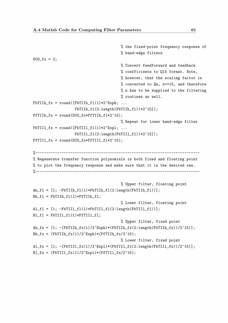
A.4 Matlab Code for Computing Filter Parameters 61
% the fixed-point frequency response of
% band-edge filters
DCG_fx = 2;
% Convert feedforward and feedback
% coefficients to Q15 format. Note,
% however, that the scaling factor is
% converted to Qn, n<=15, and therefore
% n has to be supplied to the filtering
% routines as well.
FbTIIh_fx = round([FbTIIh_fl(1)*2^Exph; ...
FbTIIh_fl(2:length(FbTIIh_fl))*2^15]);
FfTIIh_fx = round(DCG_fx*FfTIIh_fl*2^15);
% Repeat for lower band-edge filter
FbTIIl_fx = round([FbTIIl_fl(1)*2^Expl; ...
FbTIIl_fl(2:length(FbTIIl_fl))*2^15]);
FfTIIl_fx = round(DCG_fx*FfTIIl_fl*2^15);
%---------------------------------------------------------------------------
% Regenerate transfer function polynomials in both fixed and floating point
% to plot the frequency response and make sure that it is the desired one.
%---------------------------------------------------------------------------
% Upper filter, floating point
Ah_fl = [1; -FbTIIh_fl(1)*FbTIIh_fl(2:length(FbTIIh_fl))];
Bh_fl = FbTIIh_fl(1)*FfTIIh_fl;
% Lower filter, floating point
Al_fl = [1; -FbTIIl_fl(1)*FbTIIl_fl(2:length(FbTIIl_fl))];
Bl_fl = FbTIIl_fl(1)*FfTIIl_fl;
% Upper filter, fixed point
Ah_fx = [1; -(FbTIIh_fx(1)/2^Exph)*(FbTIIh_fx(2:length(FbTIIh_fx))/2^15)];
Bh_fx = (FbTIIh_fx(1)/2^Exph)*(FfTIIh_fx/2^15);
% Lower filter, fixed point
Al_fx = [1; -(FbTIIl_fx(1)/2^Expl)*(FbTIIl_fx(2:length(FbTIIl_fx))/2^15)];
Bl_fx = (FbTIIl_fx(1)/2^Expl)*(FfTIIl_fx/2^15);

Bibliography
[1] D. Brady and J. C. Preisig. Underwater acoustic communications. In H. V. Poor and
G. Wornell, editors, Wireless Communications: Signal Processing Perspectives, pages
330–379. PTR Prentice-Hall, 1998.
[2] L. Erup, F. M. Gardner, and R. A. Harris. Interpolation in digital modems —
Part II: Implementation and performance. IEEE Transactions on Communications,
41(6):998–1008, June 1993.
[3] L. Freitag, M. Johnson, and M. Stojanovic. Efficient equalizer update algorithms
for acoustic communication channels of varying complexity. In Proceedings of
OCEANS’97, pages 580–585, Halifax – Nova Scotia, Canada, October 1997.
[4] D. N. Godard. Passband timing recovery in an all-digital modem receiver. IEEE
Transactions on Communications, COM-26(5):517–523, May 1978.
[5] J. Gomes and V. Barroso. Acoustic channel equalization results for the ASIMOV
high-speed coherent data link. In Proceedings of MTS/IEEE OCEANS’00, volume 2,
pages 1437–1442, Providence, RI, September 2000.
[6] J. Gomes and V. Barroso. Digital transmission through the ASIMOV high-speed
acoustic link: Equalization results. Technical report, Institute for Systems and
Robotics — Instituto Superior Tecnico (ISR/IST), February 2000.
[7] J. Gomes and V. Barroso. Analysis of ASIMOV Toulon data. Technical report,
Institute for Systems and Robotics — Instituto Superior Tecnico (ISR/IST), October
2001.
[8] J. Gomes and V. Barroso. Equalization and coding for coherent communication in
the ASIMOV vertical link. In Proceedings of MTS/IEEE OCEANS’01, volume 4,
pages 2170–2176, Honolulu, Hawaii, November 2001.
[9] J. Gomes, V. Barroso, G. Ayela, and P. Coince. An overview of the ASIMOV acoustic
communication system. In Proceedings of MTS/IEEE OCEANS’00, volume 3, pages
1633–1637, Providence, RI, September 2000.
[10] S. Haykin. Adaptive Filter Theory. Prentice-Hall, Englewood Cliffs, NJ, third edition,
1996.
62

BIBLIOGRAPHY 63
[11] N. K. Jablon. Joint blind equalization, carrier recovery, and timing recovery for
high-order QAM signal constellations. IEEE Transactions on Signal Processing,
40(6):1383–1398, June 1992.
[12] D. B. Kilfoyle and A. B. Baggeroer. The state of the art in underwater acoustic
telemetry. IEEE Journal of Oceanic Engineering, 25(1):4–27, January 2000.
[13] E. A. Lee and D. G. Messerschmitt. Digital Communication. Kluwer Academic
Publishers, second edition, 1994.
[14] A. V. Oppenheim, A. S. Willsky, S. Hamid, and H. S. Nawab. Signals and Systems.
Prentice-Hall, Englewood Cliffs, NJ, second edition, 1996.
[15] C. B. Papadias and D. T. M. Slock. Normalized sliding window constant modulus and
decision-directed algorithms: A link between blind equalization and classical adaptive
filtering. IEEE Transactions on Signal Processing, 45(1):231–235, January 1997.
[16] J. G. Proakis. Digital Communications. McGraw-Hill Book Company, second edition,
1989.
[17] J. G. Proakis. Digital Communications. McGraw-Hill Book Company, fourth edition,
2000.
[18] B. Sklar. Digital Communications: Fundamentals and Applications. Prentice-Hall,
Englewood Cliffs, NJ, 1988.
[19] M. Stojanovic, J. A. Catipovic, and J. G. Proakis. Phase-coherent digital commu-
nications for underwater acoustic channels. IEEE Journal of Oceanic Engineering,
19(1):100–111, January 1994.
[20] O. Tanrikulu, A. G. Constantinides, and J. A. Chambers. New normalized constant
modulus algorithms with relaxation. IEEE Signal Processing Letters, 4(9):256–258,
September 1997.
[21] G. Ungerboeck. Trellis-coded modulation with redundant signal sets — Part I: In-
troduction. IEEE Communications Magazine, 25(2):5–11, February 1987.
[22] R. J. Urick. Principles of Underwater Sound. McGraw-Hill Book Company, third
edition, 1983.
[23] L.-F. Wei. Rotationally invariant trellis-coded modulations with multidimensional M-
PSK. IEEE Journal on Selected Areas in Communications, 7(9):1281–1295, December
1989.