The Art of Monetary Theory:

A New Monetarist Perspective∗

Ricardo Lagos

NYU

Guillaume Rocheteau

UC-Irvine

Randall Wright

UW-Madison, FRB Minneapolis, FRB Chicago, and NBER

July 31, 2014

∗We thank many friends and colleagues for their input, including Steve Durlauf, John Duffy,Daniela Puzzello, Andy Postlewaite, Alberto Trejos, Yiting Li, Mei Dong, Neil Wallace, Steve

Williamson, Xiaolin (Sylvia) Xiao, Mario Silva, Pedro Gomis-Porqueras, Ian King and Ricardo

Cavalcanti. Wright thanks the NSF and the Ray Zemon Chair in Liquid Assets at the Wisconsin

School of Business for research support. Lagos thanks the C.V. Starr Center for Applied Economics

at NYU and the hospitality of the Cowles Foundation for Research in Economics at Yale University,

the Federal Reserve Bank of Minneapolis, and the Federal Reserve Bank of St. Louis. The usual

disclaimers apply.

This, as I see it, is really the central issue in the pure theory of money.Either we have to give an explanation of the fact that people do holdmoney when rates of interest are positive, or we have to evade the difficultysomehow... The great evaders ... would have put it down to “frictions,”and since there was no adequate place for frictions in the rest of theireconomic theory, a theory of money based on frictions did not seem tothem a promising field for economic analysis. This is where I disagree. Ithink we have to look frictions in the face, and see if they are really sorefractory after all. Hicks (1935)

Progress can be made in monetary theory and policy analysis only bymodeling monetary arrangements explicitly. Kareken and Wallace (1980)

1 Introduction

Over the past 25 years a new approach has been developed to study monetary theory

and policy, and more broadly to study liquidity. This approach sometimes goes by

the name New Monetarist Economics.1 Research in the area lies at an interface

between macro and micro — it is meant to be empirically and policy relevant, but it

also strives for theoretical rigor and logical consistency. While most economists want

to be rigorous and consistent, we would argue that those we call New Monetarists

are more concerned with microfoundations than alternative schools in macro. And

unlike most micro theorists, they neither ignore money nor use the word as a synonym

for transferable utility. While often abstract, the research has become increasingly

oriented toward policy, partly because the theories have matured, and partly because

recent events have put monetary matters front and center, including those related to

interest rates, banking, credit conditions, financial markets and liquidity.

Papers in the area are diverse, yet share a set of principles and methods. Questions

include: What is money, why do we use it, and is it essential? Which objects will (or

should) play this role in equilibrium (or optimal) arrangements? How is intrinsically

worthless currency valued, or more generally, how can asset prices differ from “fun-

1A discussion of the New Monetarist label is contained in Williamson and Wright (2010a).

Briefly, at least some people in this camp find attractive many, but by no means all, elements of the

Old Monetarist school represented by Friedman (1960,1968,1969) and his followers. The appellation

also suggests an opposition to New Keynesian Economics, partly for its disregard for microfoun-

dations, and partly for its focus on nominal rigidities as the critical (perhaps exclusive) distortion

relevant for theoretical, empirical and policy analysis. We hope it is a constructive opposition, the

way it was good for Old Keynesians to have Old Monetarists questioning their doctrine. While we

do not want to make too much of nomenclature, we believe it is useful to get the language right

when trying to understand and differentiate alternative ways to think about monetary economics.

1

damental” values? How does credit work absent commitment? How can credit and

money coexist? What is the role of assets in credit arrangements? What are the roles

of intermediation, and of inside and outside money? What are the effects of inflation,

or monetary policy, more broadly? What is optimal policy? As should be clear, the

research is about much more than pricing currency. It is about trying to understand

the process of exchange in the presence of frictions, and how this process might be

facilitated by institutions, including money, but also credit, intermediation, and the

use of assets as payment instruments or as collateral.

A defining characteristic unifying the work discussed below is that it models the

exchange process explicitly, in the sense that agents trade with each other, at least

in some if not all situations. That is not true in GE (general equilibrium) theory,

where agents only “trade” against their budget lines. In the Arrow-Debreu paradigm,

agents are endowed with a vector x, and choose another x subject only to px ≤ px,taking as given the vector p; how they get from x to x is not up for discussion.2 The

models surveyed here go beyond classical micro by incorporating explicit frictions

that hinder interactions between agents. It is only then that one is able to analyze

how institutions ameliorate these frictions. Since money is one such institution, and

maybe the most elemental, it is natural to start there, but we do not stop there. The

focus is much broader, and includes studying any institution whose raison d’être is the

facilitation of exchange. For this one needs explicit models of the trading process.3

2Earlier work surveyed by Ostroy and Starr (1990) asked some of the right questions, but did

not resolve all the issues. Also related is work trying to use Shapley and Shubik’s (1969) market

games as a foundation for monetary economics, e.g. Hayiashi and Matsui (1996).3Others share these concerns. As regards “the old conundrum of how fiat money can survive

as an institution” Hahn (1987) says: “At a common-sense level almost everyone has an answer to

this, and old-fashioned textbooks used to embroider on some of the banalities at great length. But

common sense is, of course, no substitute for thought and certainly not for theory. In particular,

most of the models of an economy which we have, and I am thinking here of many besides those

of Arrow and Debreu, have no formal account for the exchange process.” Similarly, Clower (1970)

says: “conventional value theory is essentially a device for logical analysis of virtual trades in a

world where individual economic activities are costlessly coordinated by a central market authority.

It has nothing whatever to say about delivery and payment arrangements, about the timing or

frequency of market transactions, about search, bargaining, information and other trading costs,

or about countless other commonplace features of real-world trading processes.” On the related

topic of intermediation, Rubinstein and Wolinsky (1987) say: “Despite the important role played by

intermediation in most markets, it is largely ignored by the standard theoretical literature. This is

because a study of intermediation requires a basic model that describes explicitly the trade frictions

that give rise to the function of intermediation. But this is missing from the standard market models,

where the actual process of trading is left unmodeled.”

2

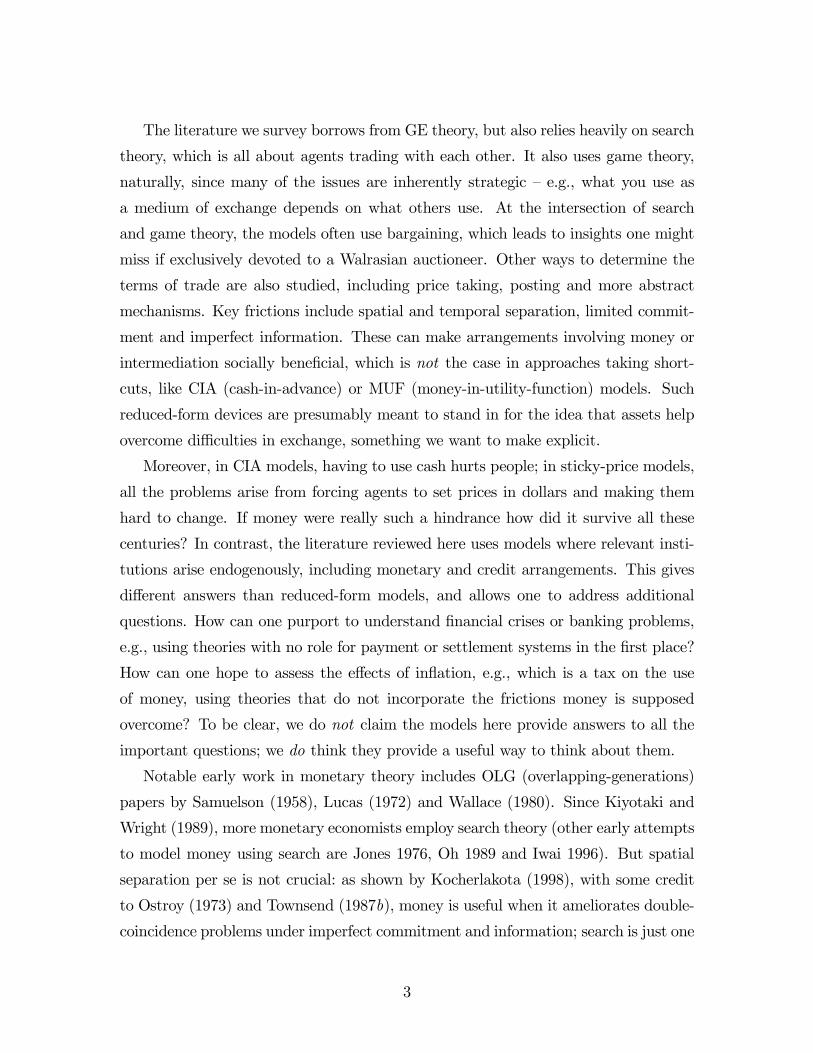
The literature we survey borrows from GE theory, but also relies heavily on search

theory, which is all about agents trading with each other. It also uses game theory,

naturally, since many of the issues are inherently strategic — e.g., what you use as

a medium of exchange depends on what others use. At the intersection of search

and game theory, the models often use bargaining, which leads to insights one might

miss if exclusively devoted to a Walrasian auctioneer. Other ways to determine the

terms of trade are also studied, including price taking, posting and more abstract

mechanisms. Key frictions include spatial and temporal separation, limited commit-

ment and imperfect information. These can make arrangements involving money or

intermediation socially beneficial, which is not the case in approaches taking short-

cuts, like CIA (cash-in-advance) or MUF (money-in-utility-function) models. Such

reduced-form devices are presumably meant to stand in for the idea that assets help

overcome difficulties in exchange, something we want to make explicit.

Moreover, in CIA models, having to use cash hurts people; in sticky-price models,

all the problems arise from forcing agents to set prices in dollars and making them

hard to change. If money were really such a hindrance how did it survive all these

centuries? In contrast, the literature reviewed here uses models where relevant insti-

tutions arise endogenously, including monetary and credit arrangements. This gives

different answers than reduced-form models, and allows one to address additional

questions. How can one purport to understand financial crises or banking problems,

e.g., using theories with no role for payment or settlement systems in the first place?

How can one hope to assess the effects of inflation, e.g., which is a tax on the use

of money, using theories that do not incorporate the frictions money is supposed

overcome? To be clear, we do not claim the models here provide answers to all the

important questions; we do think they provide a useful way to think about them.

Notable early work in monetary theory includes OLG (overlapping-generations)

papers by Samuelson (1958), Lucas (1972) and Wallace (1980). Since Kiyotaki and

Wright (1989), more monetary economists employ search theory (other early attempts

to model money using search are Jones 1976, Oh 1989 and Iwai 1996). But spatial

separation per se is not crucial: as shown by Kocherlakota (1998), with some credit

to Ostroy (1973) and Townsend (1987b), money is useful when it ameliorates double-

coincidence problems under imperfect commitment and information; search is just one

3

way to formalize this. In banking, work that fits under the New Monetarist umbrella

includes Berentsen et al. (2007) andWilliamson (2012), some of which naturally draws

on earlier research by Diamond and Dybvig (1983), Diamond (1984) and Williamson

(1986,1987). Models of intermediation and finance include Rubinstein and Wolinsky

(1987), Duffie et al. (2005) and Lagos and Rocheteau (2009). Models of credit include

Kehoe and Levine (1993) and Kiyotaki and Moore (1997). Further delineating our

approach, the idea of modeling institutions, including monetary arrangements, en-

dogenously is related to the Lucas (1976) critique, the Wallace (1998) dictum, and a

methodology espoused in Townsend (1987a,1988).4

As a preview, we start with first-generation search models of money studied by

Kiyotaki and Wright (1989,1993), Aiyagari and Wallace (1991,1992) and others, to

illustrate the tradeoff between asset returns and acceptability, and to show how

economies where liquidity plays a role are prone to multiplicity and volatility. They

can also be used to present a simplified version of Kocherlakota’s (1998) results on

the essentiality of money, and the analysis of inside and outside money in Cavalcanti

and Wallace (1999a), both of which are related to Kehoe and Levine (1993). We

then move to the second-generation models studied by Shi (1995), Trejos and Wright

(1995) and others, with divisible goods. This allows us to further explore the effi-

ciency of monetary exchange, and the idea that liquidity considerations can lead to

multiplicity and volatility. We also discuss the relation to the intermediation models

of Rubinstein and Wolinsky (1987) and Duffie et al. (2005).

We then move to divisible assets, as in the computational work of Molico (2006), or

the more tractable models Shi (1997a) and Lagos and Wright (2005). These models

are easier to integrate with mainstream macro, and thus allow us to study some

standard issues in a new light (e.g., the cost of inflation). We also discuss the effects

of monetary policy on labor markets, the interaction between money and other assets

in facilitating exchange either as a payment instrument or as collateral, and the theme

that observations that seem anomalous from the perspective of standard asset pricing

emerge naturally in models with trading frictions. Then, just as some models relax

the indivisible asset assumption in earlier search-based monetary theory, we show how

4In case readers do not know, Wallace’s dictum is this: “Money should not be a primitive in

monetary theory — in the same way that firm should not be a primitive in industrial organization

theory or bond a primitive in finance theory.”

4

Lagos and Rocheteau (2009) relax it in models of OTC (over-the-counter) markets

like Duffie et al. (2005). Finally, we discuss some information-based models.

Before getting into theory, let us clarify a few terms and put them in historical

perspective. First, when agents trade with each other, it is commonly understood

that there may be a double-coincidence problem with direct barter: in a bilateral

meeting between individuals and , it would be a coincidence if liked ’s good, and

a double coincidence if also liked ’s good.5 Next, we make reference to a medium

of exchange, for which it is hard to improve on Wicksell (1911): “an object which is

taken in exchange, not for its own account, i.e. not to be consumed by the receiver or

to be employed in technical production, but to be exchanged for something else within

a longer or shorter period of time.” Sometimes we similarly use means of payment.

Relatedly, a settlement instrument is something that discharges a debt.

Amedium of exchange that is also a consumption or production good is commodity

money. By contrast, as Wallace (1980) puts it, fiat money is a medium of exchange

that is intrinsically useless (neither a consumption nor a productive input) and incon-

vertible (not a claim redeemable in consumption or production goods). This usefully

defines a pure case, although assets other than fiat currency can convey moneyness.

Finally, one of the main challenges in monetary theory is to describe environments

where an institution like money is essential. As introduced by Hahn (1973), essential-

ity means welfare is higher, or the set of incentive-feasible allocations is larger, with

money than without it. That this is nontrivial is evidenced by the fact that money

is plainly not essential in most standard theories. As Debreu (1959) says about his

theory, an “important and difficult question ... not answered by the approach taken

here: the integration of money in the theory of value.” We hope the essay clarifies

what ingredients are relevant for understanding the issues, and how economics gets

more interesting and useful once they are incorporated.6

5Jevons’ (1875) often gets credit, but other discussions of the idea and related issues in the

history of thought include von Mises (1912), Wicksell (1911), Menger (1892) and Smith (1776).

Sargent and Velde (2003) say the first to recognize how money helps double-coincidence problems

was the Roman Paulus in the 2nd century, despite Schumpeter’s (1954) claim for Aristotle.6Related surveys or discussions include Wallace (2001,2010), Wright (2005), Shi (2006), Lagos

(2008), Williamson and Wright (2010a,b) and Nosal and Rocheteau (2011). By comparison: (i) we

discuss liquidity in general, with money a special case; (ii) we make more connections to finance and

labor; (iii) we provide simplified versions of some difficult material not in previous surveys; (iv) we

present more quantitative results. Surveys of the very different New Keynesian approach include

Clarida et al. (1999) and Woodford (2003); Gertler and Kiyotaki (2010) is somewhere in between.

5

2 Commodities as Money

We begin with Kiyotaki and Wright (1989), a model that can now be described

more easily than when it was first developed, due to advances in technique. The

goal is to derive equilibrium trading patterns endogenously, to see if they resemble

arrangements observed in actual economies, in a stylized sense, and especially to see

if there emerge institutions like the use of some commodities as media of exchange or

some agents as intermediaries.

Time is discrete and continuous forever. There is a [0 1] continuum of infinitely-

lived agents that interact according to a bilateral matching process. They have spe-

cialized tastes and technologies: there are types of agents and goods, where

agents of type consume good but produce good + 1 modulo (i.e., type

agents produce good +1 = 1). For now, the fraction of type is = 1/ , and we

set = 3. Although we usually call the agents consumers, we emphasize from the

outset that similar considerations are relevant for producers. So, instead of saying

that consumer produces good +1 but wants to consume good , it is a relabeling to

say that firm uses input and produces +1. This generates the same motives for

and difficulties with trade. However, a double-coincidence problem does nothing to

rule out credit. For that we need a lack of exogenous enforcement and commitment,

plus imperfect information, such as private trading histories. As discussed in Section

3, only under these conditions is there a need indirect trade using media of exchange.

Goods are indivisible and storable, but only 1 unit at a time. Let be the return

on good , by which we mean the flow utility agents get when they have a unit of

it in inventory. One can interpret 0 as a dividend (e.g., “fruit” from a Lucas

1978 “tree”), and 0 as a storage cost. As discussed in many places (e.g., Nosal

and Rocheteau 2011, Chapter 5), it is a venerable idea that the intrinsic properties of

objects influence which will, or should, serve as media of exchange, and storability is

the property in focus here. Type also gets utility 0 when he consumes good ,

and then produces a new unit of good +1 at cost normalized to = 0. Or, relabeling

agents as producers, one could say type use input to produce final output that is

consumed for utility . Type always accepts good in trade, and consumes it, at

least if¯¯is not too big (as discussed below, if

¯¯is too big agents may dispose of

good or hoard it for the dividend).

6

Given this, we concentrate on the following aspect of strategies: Will type trade

their production good +1 for good +2 in an attempt to facilitate future acquisition

of good ? Or will type hold onto good + 1 until it can be traded directly for

consumption? Let be the probability type trades good +1 for good +2, and let

a symmetric, stationary strategy profile be a vector τ = ( 1 2 3). If 0, type

uses good +2 as a medium of exchange. We also need to determine the distribution

of inventories. Since type consume good when they get it, they always have either

good +1 or +2. Hence,m = (123) characterizes the distribution, where

is the proportion of type holding their production good + 1. The probability per

unit time that type meets type with good + 1 is , where is the baseline

arrival rate (the probability of meeting anyone) and = 1 . The Appendix shows

how to derive the SS (steady state) condition for each type ,

+1+1 = (1−)+2+2 (1)

To describe payoffs, let be the rate of time preference and the value function

of type holding good . For convenience, let the utility from dividends be realized

next period. Then, for type 1,

12 = 2 + 2 (1−2) + 33 3+ 22 1(13 − 12) (2)

13 = 3 + 33(+ 12 − 13) (3)

which are standard flow DP (dynamic programming) equations.7 The BR (best re-

sponse) conditions are: 1 = 1 if 13 12; 1 = 0 if 13 12; and 1 = [0 1] if

13 = 12. A calculation implies 13 − 12 takes the same sign as

∆1 ≡ 3 − 2 + [33 (1− 3)− 2 (1−2)] (4)

7For those less familiar with search, consider 12. Given dividends are realized next period,

(1 + )12 = 2 + 112 + 22 [113 + (1− 1)12] + 2 (1−2) (+ 12)

+33 [3 (+ 12) + (1− 3)12] + 3 (1−3)12

The RHS is type 1’s payoff next period from the dividend, plus the expected value of: meeting his

own type with probability 1, which implies no trade; meeting type 2 with their production good

with probability 22, which implies trade with probability 1; meeting type 2 with good 1, which

implies trade for sure; meeting type 3 with good 1, which implies trade with probability 3; and

meeting type 3 with good 2, which implies no trade. Algebra leads to (2). Note also that the same

equations apply in continuous time with interpreted as a Poisson arrival rate.

7

In (4), 3−2 is the return differential from holding good 3 rather than good 2. Ifreturns were all that agents valued, this would be the sole factor determining 1. But

the other term captures the difference in the probability of acquiring 1’s desired good

when holding good 3 rather than 2, or the liquidity differential. Hence, whether 1

should opt for indirect exchange, by swapping good 2 for 3 whenever the opportunity

arises, involves comparing the return and liquidity differentials. This reduces the BR

condition for 1 to a check on the sign of ∆1. Similarly, for any ,

=

⎧⎨⎩ 1 if ∆ 0

[0 1] if ∆ = 0

0 if ∆ 0

(5)

Let V = () be the vector of value functions. Then a stationary, symmetric equi-

librium is a list hVm τ i satisfying the DP, SS and BR conditions. There are 8

candidate equilibria in pure strategies, and for each such , one can solve for , and

use (5) to determine the parameters for which is a BR to itself (see the Appendix).

To present the results, assume 1 2 0 = 3, so we can display outcomes in the

positive quadrant of (1 2) space. Figure 1 shows different regions labeled by τ to

indicate which equilibria exist. There are two cases, Model A or B, distinguished by

1 2 or 2 1.8 In Figure 1, Model A corresponds to the region below the 45 line,

where there are two possibilities: if 2 ≥ 2 the unique outcome is τ = (0 1 0); and

if 2 ≤ 2 the unique outcome is τ = (1 1 0). To understand this, note that for type

1 good 3 is more liquid than good 2. It is more liquid because type 3 accepts good 3

but not good 2, and type 3 always has what type 1 wants (3 = 1). In contrast, type

2 agents always accept good 2, but do not always have 1’s good (2 = 12). Hence,

good 3 allows type 1 to consume more quickly. If 2 2 this liquidity differential

does not compensate for a lower return; if 2 2 it does.9

In Model A, τ = (0 1 0) is what Kiyotaki and Wright call the “fundamental”

equilibrium, where good 1 is the universally-accepted commodity money, while type

8In Kiyotaki and Wright (1989), Models A and B both have 1 2, but in Model B type

produces good − 1 instead of + 1. Here we keep production fixed and distinguish A or B by

1 2 or 2 1, which is equivalent but easier. To see how they differ, consider Model A with

1 2. Then at least myopically it looks like a bad idea for type 1 to set 1 = 1, because trading

good 2 for 3 lowers his return. Similarly, it looks like a bad idea for type 3 to set 3 = 1, and a good

idea for type 2 to set 2 = 1. Hence, exactly one type is predisposed to use indirect trade based on

fundamentals. In Model B, types 2 and 3 are both so predisposed.9To see why type 1 is pivotal, note that for type 2 trading good 3 for good 1 enhances both

liquidity and return, as does holding onto good 1 for type 3. Hence, only type 1 has a tradeoff.

8

Figure 1: Equilibria with Commodities as Money

2 agents act as middlemen by acquiring good 1 from producers and delivering it

to consumers. While this may seem the most natural outcome, when 2 2 we

instead get τ = (1 1 0), called a “speculative” equilibrium, where type 1 trades the

high-return good 2 for the low-return good 3 with the expectation of better future

prospects. In this equilibrium good 1 and good 3 are both used as money. Theory

delivers cutoffs that make type 1 willing or unwilling to sacrifice return for liquidity.

Notice, however, that there is a gap between the cutoffs: for 2 2 2 there

is no stationary, symmetric equilibrium in pure-strategies; as shown, there is one in

mixed-strategies, where type 1 accepts good 3 with probability ∗ ∈ (0 1).10Things are different inModel B, above the 45 line. Given the market does not shut

down, there is always an equilibrium with τ = (0 1 1). This is the “fundamental”

equilibrium for Model B, where type 1 hang on to good 2, which now has the highest

return, while types 2 and 3 opt for indirect exchange, with goods 1 and 2 serving

as money. For some parameters, as shown, there coexists an equilibrium with τ =

(1 1 0), the “speculative” equilibrium for this specification, where goods 3 and 1 are

10See Kehoe et al. (1993). They also show there can be multiple steady-state equilibria in mixed

strategies, but the set of such equilibria is generically finite. And they construct equilibria where

1 cycles, with liquidity fluctuating over time as a self-fulfilling prophecy. Trachter and Oberfield

(2012) provide conditions under which the set of dynamic equilibria shrinks as the length of the

discrete-time period gets small. More generally, however, we argue below that economies where

liquidity plays a role are often inherently prone to multiplicity and volatility.

9

commodity monies, while good 2 is not universally accepted even though it now has

the best return. The coexistence of equilibria with different transactions patterns and

liquidity properties shows that these are not necessarily pinned down by fundamentals.

While his sums up the baseline model, there are many extensions and applica-

tions. Aiyagari and Wallace (1991) allow types and goods, prove existence of

equilibria with trade, and show there always exists one equilibrium where the best

good is universally accepted, although that is not true in all equilibria.11 Another

extension, considered in Kiyotaki and Wright (1989), Aiyagari and Wallace (1992)

and elsewhere, is to add fiat currency. We postpone discussion of this, but mention

for now that it provides one way to see that equilibria are not generally efficient: for

some parameters, equilibria with valued fiat money Pareto dominate other equilibria.

In terms of comparing different commodity-money equilibria when they coexist, it

may seem better to use the highest-return object as a medium of exchange. But at

least some agents can prefer to have other objects so used — especially those who pro-

duce the other objects, reminiscent of the bimetalism debates (see the entertaining

discussion in Friedman 1992).

To study how we might get to equilibrium, several papers use evolutionary dynam-

ics.12 In Wright (1995), in particular, there is a general population, n = (1 2 3),

which is interesting for its own sake (for some n a new equilibrium emerges). Then

agents are allowed to choose their type, interpretable as choosing preferences or tech-

nologies, or as an evolutionary process where types with higher payoffs increase in

numbers due to reproduction or imitation. In Model A, with n evolving according

to standard Darwinian dynamics, for any initial n0, and any initial equilibrium if n0

admits multiplicity, n → n∞ where at n∞ the unique equilibrium is “speculative.”

While one may have thought “fundamental” play would win out, the result can be

11Proving the existence of equilibria with trade is nontrivial because standard fixed-point theo-

rems do not guarantee a particular exchange pattern — one of Hahn’s (1965) problems. Hence, the

arguments are necessarily more involved. See also Zhu (2003,2005).12These include Matsuyama et al. (1993), Wright (1995), Luo (1999) and Sethi (1999). A related

literature, including Marimon et al. (1990) and Basçı (1999), asks if artificially-intelligent agents can

learn to play equilibrium in the model. There are also studies with real people in the lab. In terms of

these experiments, Brown (1996) and Duffy and Ochs (1999) find that subjects have little problem

getting to the “fundamental” equilibrium, but can be reluctant to adopt “speculative” strategies.

However, Duffy (2001) shows they can learn to do so. In the version with fiat money, Duffy and

Ochs (2002) find that monetary equilibria tend to get selected, and that generally it is not hard to

get objects valued for liquidity.

10

reconciled with intuition. In equilibrium with τ = (0 1 0), type 3 enjoy the highest

payoff, since they produce a good with the best return and highest liquidity. Ergo, 3

increases. And, when type 1 interact with type 3 more often, they are more inclined

to “speculate” by sacrificing return for liquidity.

Since some people find random matching unpalatable in monetary economic (e.g.,

Howitt 2005), the model has be redone with directed search. Corbae et al. (2003)

use a solution concept generalizing Gale and Shapley (1962).13 For Model A with

= 13, they find the “fundamental” outcome = (0 1 0) is the unique equilibrium

in a certain class. On the equilibrium path, starting atm = (1 1 1), type 2 trade with

3 while 1 sit out. Next period, at m = (1 0 1), type 2 trade with 1 while 3 sit out.

Then we are back atm = (1 1 1). Good 1 is always the unique money, different than

random matching. Heuristically, with random matching, in “speculative” equilibrium

type 1 is concerned with the chance of meeting type 3 with good 1. But with directed

matching, chance is not a factor: the endogenous transaction pattern is deterministic,

with type 2 catering to 1’s needs by delivering goods every second period. So, some

randomness is needed to make operative 1’s “precautionary” demand for liquidity.14

An extension by Renero (1998,1999) further studies mixed strategies. He shows

that in any equilibrium where all agents randomize, goods with lower must have

higher acceptability, and this can be socially desirable. If this is surprising, note

that to make agents indifferent between trading lower- for higher-return objects the

former must be more liquid (it is also related to Gresham’s Law). Other applications

include Camera (2001), who studies intermediation in more detail, and Cuadras-

Morató (1994) and Li (1995), who consider recognizability (information frictions) as

an alternative to storability. More can be done, but we now move to other mod-

els. We spent time on this one because it provides an early formalization of the

tradeoff between return and liquidity, and because there is no comparably accessible

presentation.

13At each , population partitions into subsets containing at most two agents (there is still bilateral

trade) such that there are no profitable deviations in trades or trading partners for any individual

or pair. While agents can choose a type to meet, it is often assumed in this approach that two

individuals still meet with probability 0.14As discussed below, there is often a reinterpretation of random matching in terms of prefer-

ence/technology shocks (as Hogan and Luther 2014 discuss explicitly in this model). Also, the results

for endogenous matching have only been established for a certain class of equilibria, for Model A,

and for = 13. It is not known what happens in Model B, with general n, or with endogenous n.

11

3 Assets as Money

Adding other assets allows us to more easily illustrate additional results. These

include: (i) assets can facilitate intertemporal exchange; (ii) this may be true for

fiat currency, an asset with a 0 return, or even assets with negative returns; (iii) for

money to be essential, necessary conditions include limited commitment and imperfect

information; (iv) the value of fiat money is both tenuous and robust; and (v) whether

assets circulate as media of exchange may not be pinned down by primitives. The

basic setup follows Kiyotaki and Wright (1991,1993), simplified it in a few ways.15

Goods are now nonstorable: they are produced on the spot, for immediate con-

sumption, at cost 0. Hence, they cannot be retraded (one can think of them as

services). Agents still specialize, but now, when and meet, the probability of a

double coincidence is , the probability of a single coincidence where likes ’s output

is , and the probability of a single coincidence where likes ’s output is . SO, e.g.,

the double-coincidence meeting rate is , with and capturing search and match-

ing, respectively. Note the equations below hold in discrete time, or in continuous

time with interpreted as a Poisson parameter. Any good likes gives him utility

; all others give him 0. There is a storable asset that no one consumes, but it

yields a dividend, i.e. flow utility . If = 0 it is fiat currency. We provisionally

assume agents neither dispose of nor hoard assets, and check it below.

In general, ∈ [0 1] is the fixed asset supply, and we continue to assume assetsare indivisible and agents can hold at most 1 unit, ∈ 0 1. To begin, however, let = 0, so that barter is the only option. The flow barter payoff is = (− ).

If 0 this beats autarky, = 0, but as long as 0 it does not do as well

as we might like: in some meetings, wants to trade but will not oblige, which is

bad for everyone in the long run. Suppose we try to institute a credit system, where

agent produces for whenever likes his output. This is called credit because agents

produce while receiving nothing by way of quid pro quo, except an understanding —

call it a promise — that someone will do the same for them in the future. The flow

15In the original model, as in Diamond (1982), agents go to one “island” to produce and another

to trade; here they produce on the spot. Also, in early versions, agents consume all goods, but like

some goods more than others, so they have to choose which to accept; here the choice is trivial.

Also, in early formulations agents with assets cannot produce, and so must use money even in

double-coincidence meetings; following Siandra (1990), here they can barter whenever they like.

12

payoff to such an arrangement is

= (− ) + − = ( + ) (− )

If 0 then . So, if agents can commit, they can promise to abide by the

credit regime, and this achieves efficiency conditional on the matching process.

If they cannot commit, promises must be credible (Kehoe and Levine 1993). This

implies an incentive-compatibility condition, IC for short. The potentially binding

condition applies to production in single-coincidence meetings. Whether this ensues

depends on the consequences of deviating. If is the deviation payoff, the IC is

−+ ≥ + (1− ) (6)

where is the probability deviators are caught and punished: 1 captures imperfect

monitoring, or record keeping, so that deviations are only probabilistically detected

and communicated to the population at large. Suppose = , so that punishment

entails a loss of future credit (one can also consider autarky). Then (6) holds iff

≤

+ ≡ (7)

Naturally, for credit to be viable the monitoring/communication technology must

be sufficiently good (i.e., cannot be too small). Suppose credit is not viable, and

consider using money. Let be the value function for agents with ∈ 0 1, andcall those with = 1 buyers and those with = 0 sellers. Then

0 = (− ) + 0 1 (1 − 0 − ) (8)

1 = (− ) + (1−) 0 1 (+ 0 − 1) + (9)

where 0 is the probability a seller is willing to produce for an asset while 1 is the

probability a buyer is willing give up an asset, and we include so the equations also

apply to real assets. If ∆ = 1 − 0, the BR conditions are:

0 =

⎧⎨⎩ 1 if ∆

[0 1] if ∆ =

0 if ∆

and 1 =

⎧⎨⎩ 1 if ∆

[0 1] if = ∆

0 if ∆

(10)

Letting V = (0 1) and τ = ( 0 1), equilibrium is a list hV τ i satisfying (8)-(10). Taking for granted 1 = 1, which as shown below is valid if || is not too big,

13

for now we only have to check the condition for 0 = 1. This reduces to

≤ (1−)

+ (1−)≡ (11)

If ≤ monetary equilibrium exists, and it yields higher welfare than barter but

lower than credit. To see this, let ≡ 1 + (1−)0, and check . Also,

notice iff 1 − . This illustrates a result in Kocherlakota (1998): if

the monitoring/record-keeping technology — what he calls memory — is perfect, in the

sense of = 1, then money is not essential. This is because = 1 implies ,

so if monetary exchange is viable then credit is, too, and . Credit is better

because with money: (i) potential sellers may have = 1; and (ii) potential buyers

may have = 0. With random matching, at least (ii) is robust.16

Figure 2: Equilibria with Assets as Money

To summarize, fiat money is inessential when = 1 but may be essential when

1 — e.g., 1 − implies , so for some money works while credit

does not. The necessary ingredients for essentiality are: (i) not all gains from trade

are exhausted by barter; (ii) there is lack of commitment; and (iii) monitoring is

imperfect.

While it can be a useful institution, fiat money is in a sense tenuous: there is

always an equilibrium where it is not valued (in Wright 1994, there are also sunspot

16Actually, with directed search, money may be as good as credit, but it cannot beat credit

(Corbae et al. 2003), unless there is some value to privacy that makes record keeping undesirable

(Kahn et al. 2005; Kahn and Roberds 2008. Also, notice from (11) and (7), does not appear in the

latter, since monetary exchange requires no record keeping. One might argue some record keeping

is always inherent in monetary exchange, because information is conveyed by the fact that one has

currency — it at least suggests having produced for someone in the past. But one could counter that

sellers do not care if buyers got assets by fair means or foul (e.g., theft); they only care about others

accepting it in the future.

14

equilibria where 0 fluctuates). Yet money is in another sense robust: equilibria with

0 = 1 exist even if 0, as long as || is not extreme. To expand on this, andto check the provisionally maintained BR condition for 1 = 1, Figure 2 shows set

of equilibrium τ = ( 0 1) for any . Equilibrium τ = (1 1) exists iff || is not toobig; τ = (0 1) exists if , in which case buyers are willing to trade assets but

sellers do not oblige; and = (1 0) exists if , in which case sellers would trade

but buyers won’t. Thus, whether the asset circulates as a means of payment is not

always pinned down by primitives: for some there coexist equilibria where it does,

and where it does not, and mixed-strategy equilibria.17

For this discussion it is important that the population is large. With a finite set

of agents, Araujo (2004) shows that even if deviations cannot be communicated to

the population at large, one can sometimes use social norms and contagion strategies

to enforce credit: if someone deviates by failing to produce for you, then you stop

producing for others, they stop producing for others, and eventually this gets back to

the first deviator. This can dissuade the original deviation if the population is small,

but not if it is large, consistent with the stylized fact that institutions like money are

used in large or complicated societies, but not always in small or primitive ones.

Even with a large population, we need imperfect monitoring, and 1 is one

just way of modeling this.18 In Cavalcanti and Wallace (1999a,b), a fraction of

the population, sometimes called bankers in applications, monitored in all meetings;

the rest, called nonbankers or anonymous agents, are never monitored. Assume that

agents can now issue notes, say, pieces of paper with names on them, with coupon

= 0, but potentially with value as media of exchange. Notes issued by anonymous

agents are never accepted by other anonymous agents in payment — why produce

to get a note when you can print your own for free? But notes issued by monitored

agents may be accepted in payment. Cavalcanti andWallace use the setup to compare

17For an arbitrary τ used by others, payoffs are 0 (τ ) and 1 (τ ), and (10) gives the BR corre-

spondence, say τ = Υ (τ ). Equilibrium is a fixed point. Notice how Υ (·) captures the idea that yourtrading strategy depends on those of others. In Figure 2, when a seller accepts he is concerned

about getting stuck with it, and when a buyer gives up he is concerned about getting stuck without

it, both of which depend on others’ strategies. This seems relevant for many assets, e.g., real estate.18The particular random monitoring formulation we use here follows Gu et al. (2013a,b). Caval-

canti and Wallace (1999a,b) have some agents monitored and not others. Sanches and Williamson

(2010) have some meetings monitored and not others. Kocherlakota and Wallace (1998) and Mills

(2008) assume information about deviations is detected with a lag. Amendola and Ferraris (2013)

assume information about deviations is sometimes lost (forgotten).

15

an outside money regime, with fiat currency and no notes, to one with inside money

with only notes, a classic issue in the design and regulation of banking systems.

The outside money regime is similar to the baseline model, except we can now

exploit the fact that some agents are monitored. Let be average utility, and for

the sake of illustration, assume monitored agents never hold money — which may

be bad for them, but for a given one can show that it does not affect . Let

us try to implement an outcome where monitored agents produce for anyone that

likes their output. To ease the presentation, set = 0 to rule out barter. Then a

monitored agent’s flow payoff is (− ), since he produces for anyone but can

only consume when he meets another monitored agent, given that anonymous agents

do not produce without quid pro quo. In some applications, monitored agents can

always become anonymous, but suppose here that they can be punished by autarky.

Then their IC is ≤ ( + ).

For anonymous agents,

0 = + (1− ) (1−) (+ 1 − 0) (12)

1 = + (1− ) (−+ 0 − 1) (13)

which modifies (8)-(9) by recognizing that they can consume but do not have to

produce when they meet monitored agent, and now denotes the asset supply per

nonmonitored agent. Generalizing (11), a monitored agent’s IC is

≤ (1− ) (1−)

+ (1− ) (1−) (14)

Welfare (average utility across monitored and nonmonitored agents) is maximized at

∗ = 12 because, as in the baseline model, this maximizes trade volume.

In the other regime, with no outside money, monitored agents can issue notes. This

allows them to consume when they meet nonmonitored agents, which is good for .

Also, one can assume that with some probability bankers require nonmonitored agents

with notes to turn them over to get goods, which can be used to adjust the supply of

notes in circulation. Again = 12 is optimal. It is easy to check is higher with

inside money, because it lets monitored agents trade more often, by issuing notes as

needed. While this may not be too surprising, the virtue of the method in general is

that it allows us to concretely discuss the relative merits of different arrangements.

16

See Mills (2008), Wallace (2010,2013,2014), Wallace and Zhu (2007) and Deviatov

and Wallace (2014) for applications.

First-generation models are crude, mainly because everything is indivisible.19 Yet

they nicely illustrate how money can be beneficial and clarify the key frictions. In

other applications, Kiyotaki and Wright (1993), Camera et al. (2003) and Shi (1997b)

endogenize specialization to show how money enhances productive efficiency. Burdett

et al. (1995) analyze who searches, buyers or sellers, while Li (1994,1995) considers

taxing money to correct search externalities. Ritter (1995), Green and Weber (1996),

Lotz and Rocheteau (2002) and Lotz (2004) consider introducing new currencies, while

Matsuyama et al. (1993) and Zhou (1997) discuss international currencies. Corbae and

Ritter (2004) analyze credit. Cavalcanti et al. (1999,2005), Cavalcanti (2004), He et

al. (2005) and Lester (2009) discuss banking. Araujo and Shevchenko (2006) and

Araujo and Camargo (2006,2008) study learning about , which is elegant because

with bilateral matching information diffuses through the population slowly. So, while

crude, the models are useful and have many implications that ring true.

4 The Terms of Trade

Second-generation monetary search theory introduced by Shi (1995) and Trejos and

Wright (1995) incorporates divisible goods and let agents negotiate over the terms of

trade. We now develop this model and use it to further illustrate how liquidity can

give rise to multiplicity and dynamics, and to say more about efficiency.

In continuous time, which makes dynamics easier, the DP equations are

0 = [ ()− ()] + 0 1 [1 − 0 − ()] + 0 (15)

1 = [ ()− ()] + (1−) 0 1 [ () + 0 − 1] + + 1 (16)

where 0 and 1 are derivatives wrt . These are like (8)-(9), except now = ()

is the utility from units of one’s consumption good and = () is the disutility

19This does drive some results. Shevchenko and Wright (2004) argue that any equilibrium with

partial acceptability, ∈ (0 1), is an artifact of nothing being divisibile. However, they go on toshow how adding heterogeneity yields a similar multiplicity and robust partial acceptability. Note

also that indivisibilities introduce a complication: as in many nonconvex environments, agents may

want to trade using lotteries, producing in exchange for a probability of getting that one can

interpret as a price (Berentsen et al. 2002; Berentsen and Rocheteau 2002; Lotz et al. 2007). This is

actually not too hard to handle, and generates some interesting results, but instead of getting into

lotteries we soon move to divisible goods.

17

of production. We impose the standard conditions: (0) = (0) = 0, 0 () 0,

0 () 0, 00 () 0 and 00 () ≥ 0 ∀ 0. Also, assume ∃ 0 with () = ().

There are two quantities to be determined in (15)-(16), in a monetary trade, and

in barter. However, since can be determined independently of , we focus on the

former; one can also simply set = 0.

Before discussing equilibrium, let’s ask what’s feasible. In Section 3, with in-

divisible goods, credit is viable iff ≤ and money iff ≤ , where =

( + ) and is the same except 1 − replaces . The analog here

is that we can support credit where agents produce for anyone that likes their out-

put ∀ ≤ and we can support exchange where agents produce for fiat money

∀ ≤ , where () = () ( + ) and the same except 1 −

replaces . Thus, IC now impinges on the intensive margin (how much agents trade).

The relevant version of Kocherlakota (1998) is this: = 1 implies . So money

is not essential when = 1, but if 1− then money is essential because we can

support some values of with money that we cannot support without it.

For equilibrium, there are many alternatives for determining the terms of trade.

Consider first Kalai’s (1977) bargaining solution, which says that when a buyer gives

an asset to a seller for , the one who entered the meeting with gets a share of

the total surplus. Since the surpluses are 1 () = () −∆ and 0 () = ∆ − (),

the Kalai solution is 1 () = 1 [ ()− ()], or

∆ = () ≡ 1 () + 0 () (17)

given the IC’s 1 () ≥ 0 and 0 () ≥ 0 hold, as they must in equilibrium.20 Giventhis, set 0 = 1 = 1 and subtract (15)-(16) to get ∆ as a function of ∆, and then

use (17) to arrive at a simple differential equation = ().21 Letting V = (0 1),

equilibrium is defined by bounded paths for hV i satisfying these conditions, with ∈ [0 ], since that is necessary and sufficient for the IC conditions. Characterizingequilibria now involves analyzing an elementary dynamical system.

20One can interpret ∆ = () as a BR condition to highlight the connection to models presented

above. Solve the DP equations for ∆ () for an arbitrary , and then, taking as given, use the

bargaining solution () = ∆ () to get = Υ () in a meeting. Equilibrium is a fixed point.

Now, one usually thinks of best responses by individuals, while here it is by pairs, but that seems a

technicality relative to the conceptual merit of connecting = Υ () to τ = Υ (τ ) in Section 3.21For the record, 0 () () = [(1 −) + 1] ()− [(1 −)− (1− 1)] ()− .

18

Figure 3: Assets as Money with Divisible Goods and High 1

Trejos and Wright (2013) characterize the outcomes, depending on 1. Figure

3 shows the case of a relatively high 1, with subcases depending on . Starting

with = 0 (middle panel), there are two steady states, = 0 and a unique 0

solving () = 0. There are also dynamic equilibria starting from any 0 , where

→ 0, due to self-fulfilling inflationary expectations. For an asset with a moderate

dividend (right panel), () shifts down, leaving a unique steady state ∈ (0 ) anda unique equilibrium, since any other solution to = () exits [0 ]. If we increase

the dividend further to (not shown), () shifts further, the steady state with

trade vanishes, and assets get hoarded. For a moderate storage cost ∈ ( 0) (leftpanel), there are two steady states with trade, ∈ (0 ) and ∈ (0 ), plusequilibria where → due to self-fulfilling expectations. For (not shown),

there is no equilibrium with trade and agents dispose of .

Multiple steady states and dynamics arise because the value of a liquid asset, real

or fiat, is partly self-fulfilling: if you think others give low for an asset then you

only give a little to get it; if you think they give high for it then you give more. Shi

(1995), Ennis (2001) and Trejos and Wright (2013) also construct sunspot equilib-

ria where fluctuates randomly over time, while Coles and Wright (1998) construct

continuous-time cycles where and ∆ revolve around steady state. These results for-

malize the notion of excess volatility in asset values, and are different from results in

ostensibly similar models without liquidity considerations (Diamond and Fudenberg

1989; Boldrin et al. 1993; Mortensen 1999), which require increasing returns in match-

ing or production. Here dynamics are due to the self-referential nature of liquidity.

Note that to get an asset sellers would incur a cost () above the “fundamental”

19

value, . This is a bubble in a standard sense: “if the reason that the price is high

today is only because investors believe that the selling price is high tomorrow — when

‘fundamental’ factors do not seem to justify such a price — then a bubble exists”

(Stiglitz 1990). One might argue liquidity services are “fundamental,” too; rather

than debate semantics, we emphasize the economics: liquidity considerations lead to

deterministic and stochastic fluctuations with preferences and technologies constant.

In terms of efficiency, clearly = ∗ desirable, where 0 (∗) = 0 (∗). Related

to Mortensen (1982) and Hosios (1990), with fiat money and a fixed , one can

construct ∗1 such that = ∗ in equilibrium iff 1 = ∗1, where ∗1 ≤ 1 iff is not

too big. Hence, if agents are patient ∗1 ≤ 1 achieves the first best; otherwise 1 = 1achieves the second best. One can also take as given and maximize wrt . If

is fixed, as in Section 3, the solution is ∗ = 12. Now, with endogenous, if ∗

then ∗ 12 because the fall in trade volume (the extensive margin) has only a

second-order cost, by the envelope theorem, while the increase in output per trade

(the intensive margin) has a first-order benefit. This captures, albeit in a stylized

way, the notion that monetary policy ought to balance liquidity provision and control

of the price level. And although of course this depends on the upper bound for , it

illustrates the robust idea that the distribution of money matters.

For a diagrammatic depiction of welfare, let 1 = () − ∆ and 0 = ∆ − ()

denote the buyer’s and seller’s surplus. Any trade must satisfy the IC’s, 1 ≥ 0

and 0 ≥ 0. The relationship between 1 and 0 as changes, the frontier of the

bargaining set, is 0 = − [−1(1 +∆)] +∆ in Figure 4. Kalai’s solution selects the

point on the frontier intersecting the ray 0 = (01)1. As 1 increases, this ray

rotates and changes 1, 0 and . Let ∗ = (∗)− (∗). In the left panel of Figure

4, assuming ∆ ≥ (∗), ∗ can be achieved for some ∗1 at the tangency between the

frontier and the 45 line. If 1 ∗1 output is too low; if 1 ∗1 it is too high. In

in the right panel, assuming ∆ (∗), output is inefficiently low for all 1, and the

second best is achieved at 1 = 1.

Many results do not rely on a particular bargaining mechanism, and various al-

ternatives are used in the literature.22 To nest these, let () be a generic mechanism

22Shi (1995) and Trejos and Wright (1995) use symmetric Nash bargaining while Rupert et

al. (2001) use generalized Nash. They consider threat points given by continuation values and by

0, both of which can be derived from strategic bargaining in a stationary setting, as in Binmore et

20

1S1S

0S0S

*S *S

*S *S

*)(qc *)(qc

11

00 SS

1

1

00 SS

1*1

*0

0 SS

*qq *qq *qq

First best

Second best

00 S

Figure 4: Proportional Bargaining and Monetary Exchange

describing how much value a buyer must transfer to a seller to get . The terms

of trade solve ∆ = (). Consider e.g. generalized Nash bargaining with threat

points given by continuation values: max [ ()−∆]1 [∆− ()]

0 . The FOC can

be written ∆ = () with

() =1

0 () () + 00 () ()

10 () + 00 () (18)

Note that (18) and (17) are the same at = ∗; otherwise, given 00 0 or 00 0,

they are different except in special cases like = 1.

As in Trejos and Wright (1995), using Nash bargaining, we can detail how effi-

ciency depends on various forces. First there is bargaining power; let’s neutralize that

by setting 1 = 12. Second there is market power, coming from market tightness,

as reflected in the threat points; let’s neutralize that by setting = 12. Then one

can show ∗, and → ∗ as → 0. The intuition is compelling: In frictionless

economies, agents work to acquire purchasing power they can turn into immediate

consumption, and hence work until 0 (∗) = 0 (∗). In contrast, in this model they

work for assets that provide consumption only in the future, when they meet the right

person. Therefore, for 0 they settle for less than ∗. This comes up with divisible

assets, too, but it is a point worth making even with ∈ 0 1.23al. (1986). Coles and Wright (1998) use the strategic solution for nonstationary equilibria. Trejos

and Wright (2013) use Kalai bargaining, which also has a strategic foundation (Dutta 2012). Others

use mechanism design (Wallace and Zhu 2007; Zhu and Wallace 2007), price posting (Curtis and

Wright 2004; Julien et al. 2008; Burdett et al. 2014) and auctions (Julien et al. 2008).23Shi (1996), Aiyagari et al. (1996), Wallace and Zhu (2007) and Zhu and Wallace (2007) study

21

5 Intermediation in Goods Markets

Intermediaries, or middlemen, like money are institutions that facilitate trade. There

are models designed to study this, and we present a well-known example due to

Rubinstein andWolinsky (1987). One reason for this is that, once we get past notation

and interpretation, their model operates much like the one in Section 4, and a service

a useful a survey can provide is to make connections between different applications.

There are three types, , and , for producers, middlemen and consumers.24

The measure of type is . There is a divisible but nonstorable good anyone can

produce at cost () = and consume for utility () = . Unlike Section 4, there

are no gains from trade in , but it can be used as a payment instrument. There are

gains from trade in a different good that is indivisible and storable: type consumes

it for utility 0, while type produces it at cost normalized to 0. While does

not produce or consume this good, he may acquire it from to trade with . It is

not possible to store more than one unit, ∈ 0 1, as above, but now the good isnot in fixed total supply since type agents have an endogenous decision to produce.

Also, holding returns are specific to and , and ≤ 0 and ≤ 0, with −and − interpreted as storage costs.

Let be the rate at which meets (subject to regularity conditions, there is

always a population n consistent with this). In matches, gives the indivisible

good to for . In matches, if has = 1 he gives it to for . In

matches, they cannot trade if = 1, and may or may not trade if = 0, but if

they do transfers to . Let be the measure of type with = 1. The

that gives splits the surplus, where is the share or bargaining power of ,

with + = 1, consistent with Nash or Kalai bargaining since () = () = .

We need to determine the fraction of that produce, , and the fraction of that

interactions between money and credit or other assets. Wallace (1997) and Katzman et al. (2003)

study money-output correlations. Johri (1999) further analyzes dynamics. Wallace and Zhou (1997)

discuss currency shortages, Wallace (2000) and Lee et al. (2005) discuss maturity and denomination

structures, while Ales et al. (2008) and Redish and Weber (2011) discuss related issues in economic

history. Williamson (1999) adds inside money. Several papers (see Section 11) add private infor-

mation. Burdett et al. (2014) study price dispersion. International applications include Curtis and

Waller (2000,2003), Wright and Trejos (2001), Camera et al. (2004) and Craig and Waller (2004).24A simplifying assumption here is that all agents stay in the market forever; the original model

had stay, while and exit after a trade, to be replaced by clones. Nosal et al. (2013) nest

these by letting agents stay with some probability after a trade.

22

actively trade, (similar to entry in Pissarides 2000). We concentrate on stationary,

pure-strategy, asymmetric equilibria, where a fraction of type and a fraction of

type are always active while the rest sit out. A key economic observation is that

since storage costs are sunk when traders meet, there are holdup problems.25

Suppose to illustrate the method that = 0, so can only trade directly with

. Then = (− ), where − is ’s surplus, since the continuation

value cancels with his outside option . Notice appears because we assume

uniform random matching, in the sense that can contact even if the latter is

not participating (imagine contacts occurring by phone, with the probability

per unit time and are connected, but only picks up if he is on the market).

Bargaining implies − = , where is total match surplus since for the

continuation value also cancels with his outside option. Then = .

Similar expressions hold for 6= 0, and for and , where the latter is ’s value

function when he has ∈ 0 1. In fact, from these DP equations, one might observethis model looks a lot like the one in Section 4, where the indivisible good was money,

except here () = () = . We said earlier can be interpreted as a payment

instrument, but one can also call the indivisible good money, since it is a storable

object acquired by and used to get from . For the record, Rubinstein and

Wolinksy (1987) call money as a synonym for transferable utility — but see Wright

and Wong (2013) for an extended discussion of this dubious practice.

In any case, the BR conditions are standard, e.g., = 1 if 0, = 1 if

∆ 0, etc. So is the SS condition. Equilibrium satisfies the obvious conditions.

From this we get the transfers in direct trade = , wholesale trade =

∆, and retail trade = + ∆. The spread, or dealer markup, is

− = + ( − )∆. Equilibrium exists and is generically unique,

as shown in Figure 5 in (− −) space. When − is high we get = 0, so the25In the original Rubinstein-Wolinsky model = 0, but there is still a holdup problem because

the transfer from to is sunk when meets . Given this, they discuss a consignment

arrangement, where transfers to only after trading with , so it is not sunk when bargaining

with . This is a example of trading institutions arising endogenously in response to frictions,

although it may or not be feasible, depending on the physical environment (it obviously does not

work if and cannot reconvene after trading, or if they can but cannot commit). In any case,

while it may alter payoffs, none of this affects efficiency in the original Rubinstein-Wolinsky setting

(see below). By contrast, the storage costs here deplete real resources — they are not just transfers

— and are necessarily sunk when or meet .

23

market is closed. When − is low and − high we get = 1 and = 0, so there

is production but no intermediation. When both are low we get intermediation. For

some parameters, enters with probability ∈ (0 1), with adjusting endogenously

to make = 0. This is related to discussions of search externalities in the literature:

here entry by does not affect the rate at which other ’s meet counterparties, it

increases , but this still makes it harder for to trade. Notice also that when

has a poor storage technology, a low rate of finding , or low bargaining power,

intermediation is essential : the market opens iff middlemen are active.

Figure 5: Equilibria with Middlemen

Rubinstein and Wolinsky (1987) use = 12 ∀ and = = 0. In that

case, is always active, and is active iff , as is socially efficient. More

generally, again related to Mortensen (1982) and Hosios (1990), in Nosal et al. (2013)

equilibrium is efficient for all values of other parameters iff = 1, = 1 and

= ∗ ∈ (0 1). For other ’s, can be too high or too low, while can betoo low but not too high. Heuristically, or are too low when or have low

bargaining power, making holdup problems severe, and can be too high due to the

above-mentioned search externality. One can say more, and there are other papers on

middlemen, including a few closely related to this survey (e.g., Li 1998, Schevchenko

2004 and Masters 2007,2008). To save space, we refer to Wright and Wong (2014) for

a longer list of citations, and turn to another application.

24

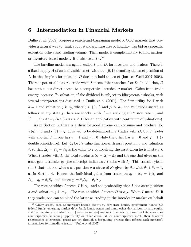
6 Intermediation in Financial Markets

Duffie et al. (2005) propose a search-and-bargaining model of OTC markets that pro-

vides a natural way to think about standard measures of liquidity, like bid-ask spreads,

execution delays and trading volume. Their model is complementary to information-

or inventory-based models. It is also realistic.26

The baseline model has agents called and , for investors and dealers. There is

a fixed supply of an indivisible asset, with ∈ 0 1 denoting the asset position of. In the simplest formulation, does not hold the asset (but see Weill 2007,2008).

There is potential bilateral trade when meets either another or . In addition,

has continuous direct access to a competitive interdealer market. Gains from trade

emerge because ’s valuation of the dividend is subject to idiosyncratic shocks, with

several interpretations discussed in Duffie et al. (2007). The flow utility for with

= 1 and valuation is , where ∈ 0 1 and 1 0, and valuations switch as

follows: in any state , there are shocks, with 0 = 1 arriving at Poisson rate 1 and

0 = 0 at rate 0 (see Gavazza 2011 for an application with continuum of valuations).

As in Section 5, there is a divisible good anyone can consume and produce, for

() = and () = . It is yet to be determined if trades with , but trades

with another iff one has = 1 and = 0 while the other has = 0 and = 1 (a

double coincidence). Let be ’s value function with asset position and valuation

, so that ∆ = 1−0 is the value to of acquiring the asset when he is in state .

When trades with , the total surplus is = ∆1−∆0 and the one that gives up the

asset gets a transfer (the subscript indicates trades with ). This transfer yields

the that entered with asset position a share of given by , with 0 + 1 = 1,

as in Section 4. Hence, the individual gains from trade are − ∆0 = 1 and

∆1 − = 0 , and hence = 0∆0 + 1∆1.

The rate at which meets is , and the probability that has asset position

and valuation is . The rate at which meets is . When meets , if

they trade, one can think of the latter as trading in the interdealer market on behalf

26“Many assets, such as mortgage-backed securities, corporate bonds, government bonds, US

federal funds, emerging-market debt, bank loans, swaps and many other derivatives, private equity,

and real estate, are traded in ... [over-the-counter] markets. Traders in these markets search for

counterparties, incurring opportunity or other costs. When counterparties meet, their bilateral

relationship is strategic; prices are set through a bargaining process that reflects each investor’s

alternatives to immediate trade.” (Duffie et al. 2007).

25

of the former for a fee. Obviously this is only relevant when meets with = 0

and = 1 or meets with = 1 and = 0, since these are the only type agents

that currently want to trade. If gets the asset, gets (for ask); if gives up an

asset, gets (for bid). Since the cost to of getting an asset on the interdealer

market is , when gives an asset to in exchange for , the bilateral surplus is

= ∆1− . And when gets an asset from the surplus is = −∆0. If

is ’s bargaining power when he deals with , then

= ∆1 + (1− ) and = ∆0 + (1− ) (19)

One can interpret − as the fee charges when he gets an asset for in the

interdealer market, and similarly for − . The round-trip spread, related to the

markup in Section 5 is = − = (∆1 −∆0) 0.

Trading strategies are summarized by τ = ( ), where is the probability

when meets with = 0 and = 1 they agree to exchange the asset for , while

is the probability when meets with = 1 and = 0 they agree to exchange

the asset for . The BR conditions are again standard, e.g. = 1 if ∆1 , etc.

The reason with = 0 and = 1 might not trade when he meets is that ≥ ∆1

is possible. Similarly, the reason with = 1 and = 0 might not trade when

he meets is that ≤ ∆0. For market clearing, because the asset is indivisible,

it will be typically the case that ∈ ∆0∆1, and the long side of the marketis indifferent to trade. If the measure of trying to acquire an asset exceeds the

measure trying to off-load one, then = = ∆1 and ∈ (0 1). In the oppositecase, = = ∆0 and ∈ (0 1). Since the measure of trying to acquire assetsis 10 and the measure trying to divest themselves of assets it 01, the former is on

the short side iff 10 01 iff ≡ 1 (0 + 1).

The SS and DP equations are standard — e.g., the flow payoff for with = 1

and low valuation is the dividend, plus the expected value of trading with or ,

plus the capital gain from a preference shock:

10 = 0 + 011 + ( −∆0) + 1 (11 − 10)

An equilibrium is a list hV τ mi satisfying the usual conditions, and it exists uniquely.The terms of trade are are easily recovered, as are variables like the bid-ask spread,

− = (1 − 0) Σ, where Σ 0. This stylized structure, with a core of

26

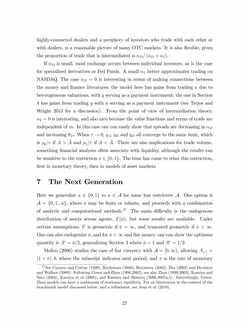
highly-connected dealers and a periphery of investors who trade with each other or

with dealers, is a reasonable picture of many OTC markets. It is also flexible, given

the proportion of trade that is intermediated is ( + ).

If is small, most exchange occurs between individual investors, as is the case

for specialized derivatives or Fed Funds. A small better approximates trading on

NASDAQ. The case = 0 is interesting in terms of making connections between

the money and finance literatures: the model here has gains from trading due to

heterogeneous valuations, with serving as a payment instrument; the one in Section

4 has gains from trading with serving as a payment instrument (see Trejos and

Wright 2013 for a discussion). From the point of view of intermediation theory,

= 0 is interesting, and also nice because the value functions and terms of trade are

independent of . In this case one can easily show that spreads are decreasing in

and increasing . When → 0, , and all converge to the same limit, which

is 0 if and 1 if . There are also implications for trade volume,

something financial analysts often associate with liquidity, although the results can

be sensitive to the restriction ∈ 0 1. The time has come to relax this restriction,first in monetary theory, then in models of asset markets.

7 The Next Generation

Here we generalize ∈ 0 1 to ∈ A for some less restrictive A. One option isA = 0 1, where may be finite or infinite, and proceeds with a combinationof analytic and computational methods.27 The main difficulty is the endogenous

distribution of assets across agents, (), but some results are available. Under

certain assumptions, is geometric if = ∞, and truncated geometric if ∞.One can also endogenize , and for ∞ and fiat money, one can show the optimum

quantity is ∗ = 2, generalizing Section 3 where = 1 and ∗ = 12.

Molico (2006) studies the case of fiat currency with A = [0∞), allowing +1 =(1 + ), where the subscript indicates next period, and is the rate of monetary

27See Camera and Corbae (1999), Rocheteau (2000), Berentsen (2002), Zhu (2003) and Deviatov

and Wallace (2009). Following Green and Zhou (1998,2002), see also Zhou (1999,2003), Kamiya and

Sato (2004), Kamiya et al. (2005), and Kamiya and Shimizu (2006,2007a,b). Interestingly, Green-

Zhou models can have a continuum of stationary equilibria. For an illustration in the context of the

benchmark model discussed below, and a refinement, see Jean et al. (2010).

27

expansion generated by a lump-sum transfer .28 As above, an agent can be a buyer

or a seller, depending on who he meets, but now he can buy whenever 0. We

maintain commitment and information assumptions precluding credit, and set = 0

to eliminate barter. Then let ( ) be the quantity of output and ( ) the

amount of dollars traded when the buyer has and the seller , assuming for

simplicity ( ) is observed by both. Then

() = (1− 2)+1 (+ )

+

Z[ ( )] + +1 [− ( ) + ] () (20)

+

Z−[ ( )] + +1 [+ ( ) + ] ()

where () is the value function of an agent with assets. The first term on the RHS

is the expected value of not trading; the second is the value of buying from a random

seller; and the third is the value of selling to a random buyer.

To determine terms of trade, consider generalized Nash bargaining,

max

( ) ( )

1− (21)

where (·) = ()++1(+−)−+1(+ ) and (·) = −()++1(++ )− +1( + ) are the surpluses. The maximization is subject to ≥ 0 and− ≤ ≤ , which might look similar to what one sees in CIA models, but they

are simply feasibility constraints, saying agents cannot hand over more than they

have (as above, credit is unavailable due to commitment and information frictions).

There is a law of motion for () with a standard ergodicity condition. A stationary

equilibrium is a list h i satisfying the obvious conditions.Molico (2006) numerically analyzes the relationship between inflation and disper-

sion in the price, (·) = (·) (·), and asks what happens as frictions decrease. Healso studies the welfare effects of inflation. Increasing by giving agents transfers

proportional to their current has no real effect — it is like a change in units. But

a lump-sum transfer 0 compresses the distribution of real balances, since when

the value of a dollar falls it hurts those with low less than those with high . Since

28This may be less relevant for real assets, but one can let stock of these assets change, say, by

having them go bad with some probability, with new ones created to keep constant. Li (1994,1995),

Cuadras-Morato (1997), Deviatov (2006) and Deviatov and Wallace (2014) do something like this

with fiat money to proxy for inflation in first- or second-generation models.

28

those with low don’t buy very much, and those with high don’t sell very much,

this compression is good for economic activity: expansionary monetary policy helps

by spreading liquidity around. At the same time, inflation detrimentally reduces real

balances, and policy must balance these countervailing effects. As Wallace (2014)

conjectures, some inflation may well desirable in any economy with such a tradeoff.

Following along these lines, Jin and Zhu (2014) study dynamic transitions for ()

after various types of monetary injections, and show how the redistributional impact

can have rather interesting effects on output and prices. They emphasize a different

effect than Molico, whereby output in a match ( ) is decreasing and convex in

, and hence, a policy that increases dispersion in real balances increases average

. This leads to slow increases in the aggregate price level after monetary injections.

The reason is not that prices are sticky — indeed, and are are determined by

bargaining in each trade — but that the increase in output keeps the nominal price

level from rising too quickly during the transition. This is very important because it

shows how Keynesian implications do not follow from time-series observations that

money shocks affect mainly output and not prices in the short run.

A different modeling approach when A = [0∞) tries to harness the distribution () somehow. One method due to Shi (1997a), assumes a continuum of households,

each with a continuum of members, to get a degenerate distribution across households.

The decision-making units are families, whose members search randomly, as above,

but at the end of each trading round they return home and share the proceeds. By a

law of large numbers, each family starts the next trading round with the same . The

approach is discussed at length by Shi (2006).29 Another method, due to Menzio et

al. (2012) and Sun (2012), uses directed search and free entry, so that while there is

a distribution (), the market segments into submarkets in such a way that agents

do not need to know ().

Here we take a different path, following Lagos and Wright (2005), which integrates

search-based models like those presented above and standard frictionless models. One

advantage is that this reduces the gap between monetary theory with some claim to

29In addition to work cited below, see Head and Kumar (2005), Head et al. (2010), Head and

Shi (2003), Kumar (2008), Peterson and Shi (2004) and Shi (2001,2005,2008,2014). Rauch (2000),

Berentsen and Rocheteau (2003b) and Zhu (2008) discuss a technical issue that comes up in large-

family models; this is avoided by the models discussed below.

29

microfoundations and mainstream macro. That this gap was big is all too clear from

Azariadis (1993): “Capturing the transactions motive for holding money balances

in a compact and logically appealing manner has turned out to be an enormously

complicated task. Logically coherent models such as those proposed by Diamond

(1982) and Kiyotaki and Wright (1989) tend to be so removed from neoclassical

growth theory as to seriously hinder the job of integrating rigorous monetary theory

with the rest of macroeconomics.” Or, as Kiyotaki and Moore (2001) put it, “The

matching models are without doubt ingenious and beautiful. But it is quite hard

to integrate them with the rest of macroeconomic theory — not least because they

jettison the basic tool of our trade, competitive markets.”

The Lagos-Wright (2005) model brings some competitive markets back on board,

to continue the nautical metaphor. But it also maintains some frictions from the

models presented above — one doesn’t want to go too far, since, as Helwig (1993)

emphasized, the “main obstacle” in developing a framework for studying monetary

systems is “our habit of thinking in terms of frictionless, organized, i.e. Walrasian

markets.” Also, realistically, one wants some of both in the same setting. Much

activity in our economic lives is quite centralized (it is easy to trade, we take prices

as given etc.) as in GE theory, but there is also much that is decentralized (it is not

easy to find counterparties, it can be hard to get credit etc.) as in search theory.

Although one might imagine different ways to combine markets with and without

frictions, Lagos and Wright try dividing each period into two subperiods: in the first,

agents interact in a decentralized market, or DM; in the second, they interact in a

frictionless centralized market, or CM.30

We now work through the details of Lagos-Wright, which has become a workhorse

in the literature. DM consumption is still denoted , while CM consumption is a

different good (we can have a vector of CM goods x without changing any key

30Some authors call the subperiods day and night as a mnemonic device; we avoid this because

it seems to bother a few people — maybe they don’t like circadian models? More substantively, we

continue to impose the frictions that make money essential, including imperfect commitment and

information. It is important to recognize that the presence of a CM does not logically imply agents

can communicate DM deviations to the population at large, even if one may get that impression

from Aliprantis et al. (2006,2007a). To clarify their contribution, they give agents the ability to

communicate DM deviations when they reconvene in the CM, which is is a legitimate assumption,

but so is the assumption that they cannot communicate deviations. Moreover, even given their

formulation, in Aliprantis et al. (2007b) they show how to ensure money is still essential. There is

more to be done on these issues; see Araujo et al. (2012) for recent developments.

30

results). For now, is produced one-for-one using labor , so the CM real wage

is 1. As above, in the DM, households can end up as buyers or sellers depending

on who they meet. In the former case their period utility is U ( 1− ) + (),

while in the latter case it is U ( 1− )− (), where U (·) is monotone and concavewhile (·) and (·) are as in Section 4. For ease of presentation, let us begin withU ( 1− ) = ()− and discuss alternatives later. In the DM, the value function

(·) is described by (20) with one change: wherever +1(·) appears on the RHS,replace it with (·), since before going to the next DM agents now visit the CM,

where (·) is the value function. It satisfies

() = max

()− + +1() st = (− ) + + +

where and are asset holdings when trading opens and closes, is the price of

in terms of , is a dividend, and denotes any other purchasing power.31

There are constraints ≥ 0, ≥ 0 and ∈ [0 1] that we ignore for now. Then,eliminating , we have

() = (+ ) + +max()− +max

−+ +1() (22)

Several results are immediate: (i) = ∗ is pinned down by 0(∗) = 1; (ii) () is

linear with slope + ; and (iii) is independent of wealth. By (iii) we get history

independence ( is orthogonal to ), and hence () is degenerate when there is a

unique maximizer . In most applications there is a unique such . In some, like

Galenianos and Kircher (2008) or Dutu et al. (2012), is nondegenerate for endoge-

nous reasons, but the analysis is still tractable due to history independence. Similarly,

with exogenous heterogeneity (see below), is only degenerate after conditioning on

type, but that is enough for tractability.

It is important to know these results actually hold for a larger class of specifica-

tions. Instead of quasi-linear utility, we can assume U ( 1− ) is homogeneous of

degree 1, as a special case of Wong (2012), and hence we can use common prefer-

ences like (1− )or [ + (1− )

]1. Alternatively, as shown in Rocheteau et

al. (2008), the main results all go through with any monotone and concave U ( 1− )

31This includes transfers net of taxes. Note also that instead of injecting new money via transfer

, in this model, government can buy CM goods and nothing changes but . We mention this in

case one worries about the realism of lump-sum money transfers.

31

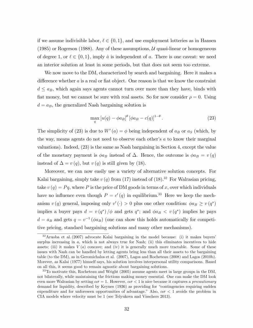
if we assume indivisible labor, ∈ 0 1, and use employment lotteries as in Hansen(1985) or Rogerson (1988). Any of these assumptions, U quasi-linear or homogeneousof degree 1, or ∈ 0 1, imply is independent of . There is one caveat: we need

an interior solution at least in some periods, but that does not seem too extreme.

We now move to the DM, characterized by search and bargaining. Here it makes a

difference whether is a real or fiat object. One reason is that we know the constraint

≤ , which again says agents cannot turn over more than they have, binds with

fiat money, but we cannot be sure with real assets. So for now consider = 0. Using

= , the generalized Nash bargaining solution is

max[()− ]

[ − ()]

1− (23)

The simplicity of (23) is due to 0 () = being independent of or (which, by

the way, means agents do not need to observe each other’s to know their marginal

valuations). Indeed, (23) is the same as Nash bargaining in Section 4, except the value

of the monetary payment is instead of ∆. Hence, the outcome is = ()

instead of ∆ = (), but () is still given by (18).

Moreover, we can now easily use a variety of alternative solution concepts. For

Kalai bargaining, simply take () from (17) instead of (18).32 For Walrasian pricing,

take () = , where is the price of DM goods in terms of , over which individuals

have no influence even though = 0 () in equilibrium.33 Here we keep the mech-

anism () general, imposing only 0 (·) 0 plus one other condition: ≥ (∗)

implies a buyer pays = (∗) and gets ∗; and (∗) implies he pays

= and gets = −1 () (one can show this holds automatically for competi-

tive pricing, standard bargaining solutions and many other mechanisms).

32Aruoba et al. (2007) advocate Kalai bargaining in the model because: (i) it makes buyers’

surplus increasing in , which is not always true for Nash; (ii) this eliminates incentives to hide

assets; (iii) it makes () concave; and (iv) it is generally much more tractable. Some of these

issues with Nash can be handled by letting agents bring less than all their assets to the bargaining

table (to the DM), as in Geromichalos et al. (2007), Lagos and Rocheteau (2008) and Lagos (2010b).

Morever, as Kalai (1977) himself says, his solution involves interpersonal utility comparisons. Based

on all this, it seems good to remain agnostic about bargaining solutions.33To motivate this, Rocheteau and Wright (2005) assume agents meet in large groups in the DM,

not bilaterally, while maintaining the frictions making money essential. One can make the DM look

even more Walrasian by setting = 1. However, 1 is nice because it captures a precautionary

demand for liquidity, described by Keynes (1936) as providing for “contingencies requiring sudden

expenditure and for unforeseen opportunities of advantage.” Also, 1 avoids the problem in

CIA models where velocity must be 1 (see Telyukova and Visschers 2013).

32

For any such (), the DM value function satisfies

() = () + [()]− +

Z− [()] () (24)

where is money held by an individual while is held by others, which we allow to

be random at this stage, although in equilibrium = . Then one can easily derive

0() = + 0[()]0()− =

½1 +

0 [ ()]0 [ ()]

−

¾

using 0() = 0 (), which follows from = (). We now insert this into the

FOC from the previous CM, −1 = 0 (), where the −1 subscript indicates lastperiod. The result is the Euler equation

−1 = [1 + ()] (25)

where () ≡ 0 () 0 ()− 1 is the liquidity premium, or equivalently, the Lagrangemultiplier on the constraint in the problem max ()− () st () ≤ .

Although we focus mainly on stationary equilibrium, for the moment let’s proceed

more generally. Using = (), = , and = (1 + )−1, (25) becomes

(1 + ) (−1) = () [1 + ()] (26)

Given any path for , one can study dynamics as in Section 4. Various authors have

shown there can be cyclic, chaotic and stochastic equilibria, again due to the self-

referential nature of liquidity (Lagos and Wright 2003; Ferraris and Watanabe 2011;

Rocheteau and Wright 2013; Lagos and Zhang 2013; He et al. 2013).

In a stationary equilibrium = is constant, so +1 = 1 + is the gross

inflation rate — a version of the Quantity Theory. To present the results compactly,

let be the interest rate on an illiquid nominal bond, i.e., one that cannot be traded

in the DM for whatever reason, or simply as an accounting exercise asking how much

money you would pay in the CM to get a dollar in the next CM. The logic behind

the Fisher equation implies 1 + = (1 + ) (1 + ), where is the interest rate on an

illiquid real bond. So policy can be described by , and (25) reduces to

= () (27)

Given , (27) determines . Real balances are = () and the price level is 1 =

() — another version of the Quantity Theory. The FOC from the CM determines

, and comes from the budget equation to complete equilibrium.34 There is a

34For individuals, CM labor depends on , say (), but in aggregate =R () = .

33

unique such equilibrium if 0 () 0. For many mechanisms, but not all, 0 () 0 is

automatic (e.g., Kalai and Walras, but not generalized Nash). However, even without

0 () 0Wright (2010) shows that there is generically a unique stationary monetary

equilibrium, with natural properties like 0, 0 etc.

As for efficiency, for generalized Nash bargaining, Lagos and Wright (2005) show

= ∗ under two conditions (see also Berentsen et al. 2007). The first is the Friedman

rule = 0, which eliminates the usual intertemporal wedge in money demand. The

second is = 1, again related to Mortensen (1982) and Hosios (1990). Heuristically,

when agents bring money to the DM they are making an investment in liquidity, and

they underinvest if they do not get the appropriate return. With Nash bargaining

this means = 1. If 1 is immutable, it would seem desirable to set 0,

but that is not feasible, since there is no equilibrium with 0. This is a New

Monetarist version of the zero-lower-bound problem currently emphasized in New

Keynesian circles. Although here it has nothing to do with nominal rigidities, it can

still be ascribed to a poor pricing mechanism — e.g., Kalai bargaining with any 0

delivers ∗ at = 0 (Aruoba et al. 2007).35 We return to this in Section 9.

That’s the basic model. While one can relax any of our assumptions, something

like quasi-linearity or the options mentioned above is needed for history independence.

Without that, the model is well posed and (even more) interesting, but requires nu-

merical methods, as in Chiu and Molico (2010,2011). By analogy, while specifications

with heterogeneity and incomplete markets are worth studying computationally in

mainstream macro, it is nice to have standard growth theory as a benchmark to an-

alyze existence, uniqueness or multiplicity, dynamics, efficiency, etc. For monetary

economics, the framework just presented is our benchmark.

8 Extending the Benchmark

Some versions of our baseline environment have the CM and DM open simultaneously

with agents transiting randomly between them (Williamson 2007); others have mul-

tiple rounds of DM trade between CM meetings or vice-versa (Berentsen et al. 2005;

35One can also design a mechanism (·) that for some parameters delivers ∗ even at 0, as

in Hu et al. (2009). This is relevant because = 0 requires deflation, = − 1 0, which typicallyrequires taxation. As Andolfatto (2013) argues, the assumptions that make money essential can also

make it difficult to enforce taxes.

34

Telyukova and Wright 2008; Ennis 2009); others use continuous time (Craig and

Rocheteau 2008b; Rocheteau and Rodriguez 2013). An extension in Lagos and Ro-

cheteau (2005) and Rocheteau and Wright (2005), on which we spend more time, has

two distinct types, called buyers and sellers because in every DM the former want

to consume but cannot produce while the latter produce but do not consume. One

cannot do this with only DM trade — why work for money if there is no occasion to

spend it? But here sellers produce in the DM and spend the receipts in the CM. This

makes the DM a two-sided market, with distinct ex ante types, buyers and sellers, as

opposed to traders that can be either depending on meetings, which makes it more

natural to incorporate general matching technologies and participation decisions.36

A two-sided market also makes it natural to consider competitive search, where

market makers set up submarkets in the DM to attract buyers and sellers and charge

them entrance fees.37 Normalize the measure of buyers to 1 and let be the measure of

sellers. In general, they meet in the DM according to a standard matching technology,

where () is the probability a buyer meets a seller and () is the probability a

seller meets a buyer. A submarket involves posting ( ) in the CM, describing the

next DM by the terms of trade — buyers and sellers commit to swapping units of

output for = real balances if they meet — as well as the seller-buyer ratio that

agents use to compute the probability of meeting. Market makers design ( ) to

maximize buyer’s surplus subject to sellers getting a minimal surplus, or vice-versa.

In equilibrium, surpluses are dictated by the market.

Algebra reduces the market maker problem to

max

() [ ()− ]− st () [ − ()] =

given the seller’s surplus . Eliminating and taking the FOC’s, we get

()0 () = [ () + ]0 () (28)

0 () [ ()− ()] =

∙1 +

(1− )

()

¸ (29)

36By analogy, Pissarides (2000) is a two-sided market with workers and firms; Diamond (1982) is

a one-sided market. The former is able to use matching functions with arrival rates depending on

market tightness and entry, which is interesting even with constant returns; the latter is not.37In equilibrium, the fee is 0. This market maker story comes from in Moen (1997) and Mortensen

and Wright (2002). We can instead let sellers post terms of trade to attract buyers or vice-versa;

sometimes these are equivalent, sometimes not (Faig and Huangfu 2007). Monetary models with

competitive search, in addition to those discussed below, include Faig and Jerez (2006), Huangfu

(2009), Dong (2011), Dutu et al. (2011) and Bethune et al. (2014).

35

where = 0 () () is the elasticity of the matching function wrt participation

by sellers. One can assume all agents participate in the DM for free, so that is

given. Then (28) determines , while (29) determines and hence also . Or one

can assume sellers have a cost to enter the DM payable in the next CM. Then

= , and (28)-(29) determine and jointly. In either case, = 0 implies = ∗,

and given this, with endogenous entry, it implies 0 (∗) [ (∗)− (∗)] = .38

Lagos and Rocheteau (2005) fix but endogenize buyers’ search intensity. They

first show that with bargaining the time it takes buyers to spend their money increases

with , counter to the well-known “hot potato” effect of inflation (e.g., see Keynes

1924, p. 51). This is because , as a tax on money, reduces the DM surplus and hence

search. But with competitive posting, although lowers the total surplus, for some

parameters it raises buyers’ share. Hence, they can get buyers to spend money faster

at higher by having them increase search effort. Alternatively, Liu et al. (2011)

get buyers to spend their money faster at higher , even with bargaining, by giving

buyers rather than sellers a participation decision. In this case, makes them match

faster by reducing buyer entry, given a standard matching technology. Alternatively,

in Nosal (2011) makes buyers spend faster by reducing their reservation trade. See

also Ennis (2009) and Hu et al. (2014). We find these exercises insightful because they

concern duration analysis, something for which search models are well suited while

reduced-form models are, in a word, useless.

Rather than permanently distinct types, it is equivalent to have type determined

each if the realization occurs before the CM closes — (27) still holds, with agents

conditioning on all the information they have when they choose . Related to this,

Berentsen et al. (2007) introduce banking. After the CM closes, but before the DM

opens, agents realize if they will be buyers or not, at which point banks are open where

they can take money out while others put it in. Or, to make it look more like standard

deposit banking, we can say everyone puts money in the bank in the CM, and when

types are revealed buyers withdraw while others leave their accounts alone. Thus,

38Comparing this to the planner’s problemmax () [ ()− ()]− , it is easy to see thatwith competitive search = 0 achieves efficiency on the intensive and extensive margins, (∗ ∗).In contrast, consider Kalai bargaining with DM entry by sellers. It is not hard to show this yields

∗ iff 1− = 0 (∗)∗ (∗), the Hosios condition saying that sellers’ share of the surplus shouldequal the elasticity of the matching function wrt their participation. Since competitive search yields

(∗ ∗) automatically at = 0, some say that it generates the Hosios condition endogenously.

36

a bank contract involves an option to convert interest-bearing deposits into cash (or

to transfer the claim to a third party) on demand. This enhances efficiency because

nonbuyers can earn interest on balances that would otherwise lay idle, with interest

payments covered by what buyers pay for loans. Hence, banks reallocate liquidity

towards those that could use more, similar to Diamond-Dybvig (1983), although here

bankers realistically take deposits and make loans in cash rather than goods.

IN some applications, bankers can abscond with deposits or borrowers renege on

debt (Berentsen et al. 2007). Others study the role of banks in investment and growth

(Chiu and Meh 2011; Chiu et al. 2013). Related work includes Li (2006,2011), He et

al. (2008), Becivenga and Camera (2011) and Li and Li (2013). In some of these,

money and banking are complements, since a bank is where one goes to get cash; in

others, they are substitutes, since currency and bank liabilities are alternative pay-

ment instruments, allowing one to discuss not only currency but checks or debit cards.

Ferraris and Watanabe (2008,2011,2012) and He et al. (2013) have versions with in-

vestment in capital or housing used to secure cash loans from banks; as discussed

below, in these models investment can be too high and endogenous dynamics can

emerge. Williamson (2012,2013,2014) has models where banks design contracts like

Diamond-Dybvig, incorporating multiple assets and private information. His banks

hold diversified portfolios that allow depositors to share in the benefits of long-term

investing with less exposure to liquidity shocks.39

Returning to participation, one can allow entry into the DM by sellers or buyers,

or have a fixed population that choose to be one or the other (Rocheteau and Wright

2009; Faig 2008). This illustrates how search externalities might make 0 desirable.

Aruoba et al. (2007) show that entry can be excessive, in which case 0 can raise

welfare. This is important because it is a common misperception that = 0 is always

39Gu et al. (2013a) develop a related theory of banking based on limited commitment. Agents

have various combinations of attributes affecting the tightness of their IC. This determines who

should be a banker, which means accepting and investing deposits. Banking can be essential in the

same sense money can be (see also Araujo and Minetti 2011). Monitoring can also be endogenized,

as in Diamond (1984). What is more novel is that agents use bank liabilities (claims on deposits) to

facilitate transactions with third parties, as inside money. That this is perhaps the most commonly

understood role of banking is clear from Selgin (2007): “Genuine banks are distinguished from other

kinds of . . .financial intermediaries by the readily transferable or ‘spendable’ nature of their IOUs,

which allows those IOUs to serve as a means of exchange, that is, money. Commercial bank money

today consists mainly of deposit balances that can be transferred either by means of paper orders

known as checks or electronically using plastic ‘debit’ cards.”

37

optimal in this class of models; that is false once there are trading frictions and

externalities. And these are not trite examples, like saying that inflation is good

because it taxes cash goods, like cigarettes, and someone has decided people smoke

too much. That is trite because, without further assumptions, we can tax smoking

directly. Relatedly, in New Keynesian models, deviations from the Friedman rule

are due to nominal rigidities, but they can instead be addressed with fiscal policy

(Correia et al. 2008). New Keynesian prescriptions of 0 follow from maintained

inefficiencies, sticky prices, just as ours follow from congestion externalities, in both

cases under the assumption that fiscal policy is not available.

We can add heterogenous DM meetings. Consider a random variable , such that

when a buyer meets a seller the former gets utility () from the latter’s goods.

This illustrates further differences between the models here and ones with exogenous

trading patterns, and how a strict lack of double coincidence meetings is not needed

for money to be valued. Suppose in every meeting and like each other’s output,

but it may be asymmetric, 6= . With pure barter, where gets from and

gets from , it is easy to verify that efficiency entails whenever .

But bargaining yields the opposite, because drives a harder bargain when really

likes his wares (to say it differently, is really expensive in terms of when does

not like ’s goods very much). In a monetary economy, can pay in as well as , and

this improves his terms of trade. Here agents choose to use cash not because barter

is impossible, but because it is coarse.40

We can also make the money supply random. Suppose = (1 + )−1, where

is drawn at the start of the DM The to be implemented later that period generally

affects , and hence , but agents do not know it when they chose . Thus, agents

equate the cost and expected benefit of liquidity. It is still optimal to have = 0, but

this is no longer equivalent to a unique money supply rule: a given is consistent with

any stochastic process for with the same [1(1 + )]. Lagos (2010a) characterizes

the general class of monetary policies consistent with = 0. If ≤ binds in every

state, the results look like those in Wilson (1979) or Cole and Kocherlakota (1998)

40This approach was used in second-generation models by Engineer and Shi (1998,2001),

Berentsen and Rocheteau (2002) and Jafarey and Masters (2003). Our presentation is based on

Berentsen and Rocheteau (2003a). Relatedly, in Jacquet and Tan (2011,2012), money is more liquid

than real assets with state-dependent dividends, since those are valued differently by agents with

different hedging needs, while cash is valued uniformly.

38

for deterministic CIA models. See also Nosal and Rocheteau (2011), where buyers

and sellers can be asymmetrically informed about inflation.

Another extension adds capital, although that can raise questions about competi-

tion between and , addressed in Section 10. Here as in Aruoba and Wright (1993)

we assume is not portable — cannot be taken to the DM — and claims to are not

recognizable — they can be forged. So cannot be a medium of exchange. The CM

production function is now ( ), and the DM cost function ( ). Then

( ) = max

n()− + +1( )

o(30)

st + = (− ) + (1− ) + [1 + ( − ) (1− )] +

where and are factor prices, and are tax rates and is the depreciation

rate. The FOC’s imply ( ) is independent of, and is linear in, ( ), generalizing

our benchmark results. The setup also nests conventional macro: if () = log ()

and ( ) is Cobb-Douglas, nonmonetary equilibrium is exactly Hansen (1985).

As in Aruoba et al. (2011), at the start of the DM, assume preference/technology

shocks determine which agents want to buy or sell. Then buyers search, while sellers

sit on their and wait for buyers to show up, consistent with capital not being

portable. The DM terms of trade satisfy ( ) = (1− ), where ( )

comes from, say, Nash bargaining. It is not hard to derive the Euler equations for

and . Combining these with the other equilibrium conditions, we get

(1 + ) ( ) = (+1 +1) [1 + (+1 +1)] (31)

0() = 0(+1) 1 + [1(+1 +1)− ] (1− )−(+1 +1) (32)

0() = 1 (1− ) 1( ) (33)

+ = ( ) + (1− ) − +1 (34)

where (·) ≡ [2(·)− 1 (·) 2(·)1(·)]. Given policy and 0, equilibrium is a

path for ( ) satisfying (31)-(34).

A novelty compared to standard macro is the term (·) in (32), which reflectsa holdup problem in the demand for capital, parallel to the one in the demand for

money. The first problem is avoided iff = 0 and the second iff = 1; for intermediate

there is underinvestment in both and , which has implications for welfare and

the model’s empirical performance. With bargaining, reduces investment by only

39

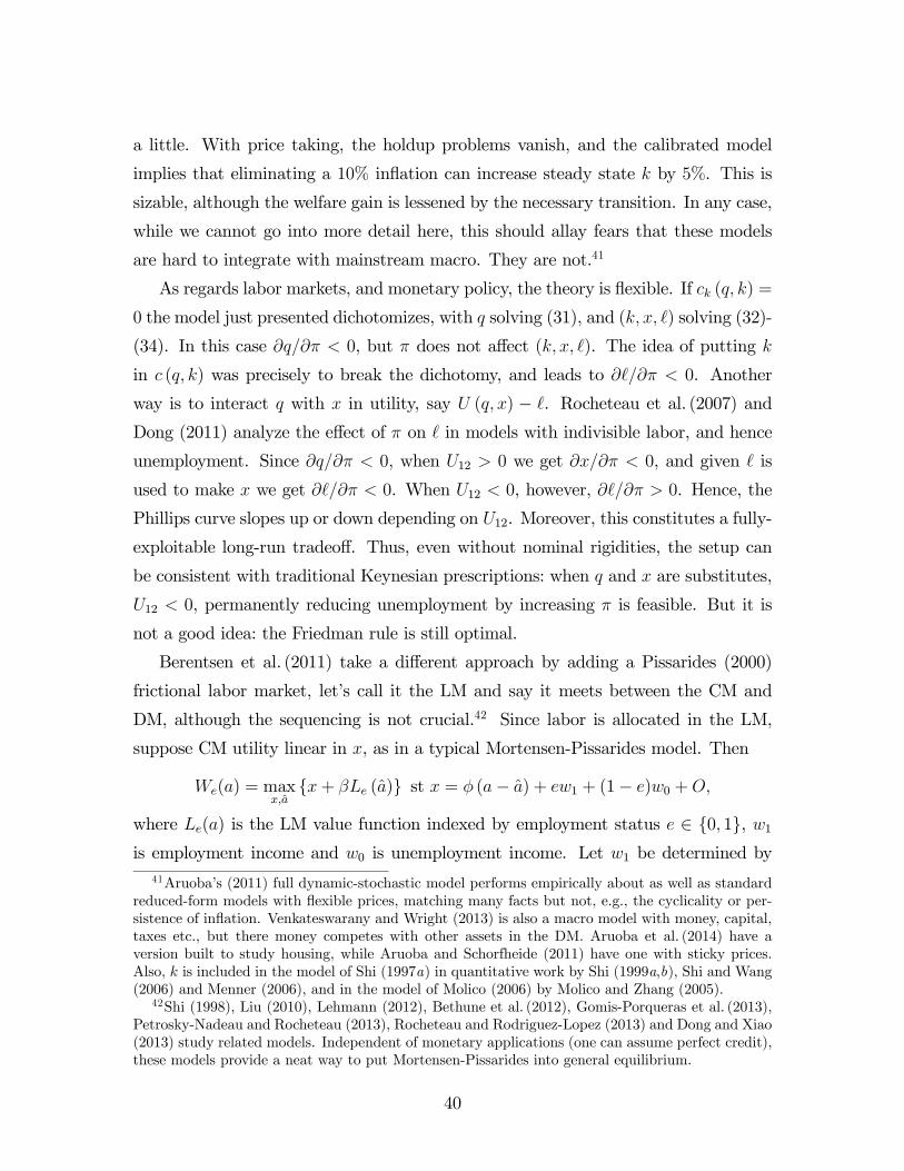
a little. With price taking, the holdup problems vanish, and the calibrated model

implies that eliminating a 10% inflation can increase steady state by 5%. This is

sizable, although the welfare gain is lessened by the necessary transition. In any case,

while we cannot go into more detail here, this should allay fears that these models

are hard to integrate with mainstream macro. They are not.41

As regards labor markets, and monetary policy, the theory is flexible. If ( ) =

0 the model just presented dichotomizes, with solving (31), and ( ) solving (32)-

(34). In this case 0, but does not affect ( ). The idea of putting

in ( ) was precisely to break the dichotomy, and leads to 0. Another

way is to interact with in utility, say ( ) − . Rocheteau et al. (2007) and

Dong (2011) analyze the effect of on in models with indivisible labor, and hence

unemployment. Since 0, when 12 0 we get 0, and given is

used to make we get 0. When 12 0, however, 0. Hence, the

Phillips curve slopes up or down depending on 12. Moreover, this constitutes a fully-

exploitable long-run tradeoff. Thus, even without nominal rigidities, the setup can

be consistent with traditional Keynesian prescriptions: when and are substitutes,

12 0, permanently reducing unemployment by increasing is feasible. But it is

not a good idea: the Friedman rule is still optimal.

Berentsen et al. (2011) take a different approach by adding a Pissarides (2000)

frictional labor market, let’s call it the LM and say it meets between the CM and

DM, although the sequencing is not crucial.42 Since labor is allocated in the LM,

suppose CM utility linear in , as in a typical Mortensen-Pissarides model. Then

() = max

+ () st = (− ) + 1 + (1− )0 +

where () is the LM value function indexed by employment status ∈ 0 1, 1is employment income and 0 is unemployment income. Let 1 be determined by

41Aruoba’s (2011) full dynamic-stochastic model performs empirically about as well as standard

reduced-form models with flexible prices, matching many facts but not, e.g., the cyclicality or per-

sistence of inflation. Venkateswarany and Wright (2013) is also a macro model with money, capital,

taxes etc., but there money competes with other assets in the DM. Aruoba et al. (2014) have a

version built to study housing, while Aruoba and Schorfheide (2011) have one with sticky prices.

Also, is included in the model of Shi (1997a) in quantitative work by Shi (1999a,b), Shi and Wang

(2006) and Menner (2006), and in the model of Molico (2006) by Molico and Zhang (2005).42Shi (1998), Liu (2010), Lehmann (2012), Bethune et al. (2012), Gomis-Porqueras et al. (2013),

Petrosky-Nadeau and Rocheteau (2013), Rocheteau and Rodriguez-Lopez (2013) and Dong and Xiao

(2013) study related models. Independent of monetary applications (one can assume perfect credit),

these models provide a neat way to put Mortensen-Pissarides into general equilibrium.

40

bargaining in the LM, but paid in the CM, without loss in generality. Thus is

independent of , and also of . Unemployed agents in the LM find jobs at a rate

determined by a matching function taking unemployment and vacancies as inputs.

In the DM, worker-firm pairs produce output, but agents do not consume what

they produce. Instead, all households and a measure of firms participate in the DM,

where is the employment rate and hence also the measure of firms with workers. the

DM arrival rate is determined by a matching function taking as inputs the measures

of buyers and sellers. This establishes a connection between the LM and DM: higher

allows buyers to trade more frequently, endogenizing the need for liquidity (something

that is exogenous in many models). Thus, higher leads to higher . A second link

between is that higher leads to higher DM revenue for firms, which leads to more

vacancies and higher employment. By taxing real balances, inflation lowers , and this

adversely affects employment. Smoothed unemployment rates are shown in Figure 6

from the data and a calibrated dynamic-stochastic version of Berentsen et al. (2011),

generated by feeding in actual monetary policy, and assuming productivity, taxes etc.

are constant. While it obviously cannot match every wiggle, and certainly misses the

60’s, theory tracks broad movements in unemployment quite well.

Figure 6: Unemployment: Model and Data

To be clear, despite lingering faith by some in a downward sloping Phillips curve,

unemployment and inflation in US data are positively correlated, except maybe at

very high frequencies or in subperiods like the 60’s. In Figure 7, the left and right

panels show unemployment against and for raw data and filtered data, color

41

coded by decade (e.g., one can see the downward-sloping pattern of the 60’s in pink).

While the panels are similar, the one on the right is probably more relevant, since what

really matters in the theory is expected inflation, and for that may better proxy than

contemporaneous . In any case, the relationship is positive in both panels. If one

prefers more advanced time-series econometric methods, see Haug and King (2014),

from which we display their remarkable Figure 8 on inflation and unemployment with

a phase shift of 13 quarters. In terms of the Old Monetarist notion of “long and

variable lags” between policy and outcomes, Figure 8 suggests they may be long, but

they are not especially variable.43

Figure 7: Scatters of Unemployment vs and

The framework can also explain nominal rigidities, as in Head et al. (2012), where

the model matches well the micro evidence on price changes, but has implications

very different from Keynesianism. The key ingredient is to replace bargaining in the

DM with price posting à la Burdett and Judd (1983). This means each seller sets

taking as given the distribution of other prices, say (), and the behavior of buyers.

The idea in Burdett-Judd is that the law of one price fails when some buyers see 1

and others see more than 1 price at a time. This delivers an endogenous () on

43Our findings are also related to Old Monetarism in other ways. Friedman (1968) says there may

be a trade-off between inflation and unemployment in the short run, but in the longer run the latter

gravitates to its “natural rate.” Friedman (1977) says “This natural rate will tend to be attained

when expectations are on average realized ... consistent with any absolute level of prices or of price

change, provided allowance is made for the effect of price change on the real cost of holding money

balances.” This is the effect explicit in the above models. The data in Friedman (1977) suggested

to him an upward-sloping Phillips curve, too, but certainly not as remarkablly as Figure 8.

42

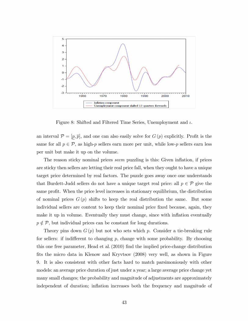
Figure 8: Shifted and Filtered Time Series, Unemployment and .

an interval P = [ ], and one can also easily solve for () explicitly. Profit is thesame for all ∈ P, as high- sellers earn more per unit, while low- sellers earn lessper unit but make it up on the volume.

The reason sticky nominal prices seem puzzling is this: Given inflation, if prices

are sticky then sellers are letting their real price fall, when they ought to have a unique

target price determined by real factors. The puzzle goes away once one understands

that Burdett-Judd sellers do not have a unique target real price: all ∈ P give the

same profit. When the price level increases in stationary equilibrium, the distribution

of nominal prices () shifts to keep the real distribution the same. But some

individual sellers are content to keep their nominal price fixed because, again, they

make it up in volume. Eventually they must change, since with inflation eventually

∈ P, but individual prices can be constant for long durations.Theory pins down () but not who sets which . Consider a tie-breaking rule

for sellers: if indifferent to changing , change with some probability. By choosing

this one free parameter, Head et al. (2010) find the implied price-change distribution

fits the micro data in Klenow and Kryvtsov (2008) very well, as shown in Figure

9. It is also consistent with other facts hard to match parsimoniously with other

models: an average price duration of just under a year; a large average price change yet

many small changes; the probability and magnitude of adjustments are approximately

independent of duration; inflation increases both the frequency and magnitude of

43

Figure 9: Price Change Distribution: Model and Data

changes; and inflation increases the positive fraction and reduces the negative fraction.

But one cannot exploit this stickiness by policy. Different from models with ad hoc

rigidities, a one-time increase in is met with a shift in () that leaves all real

variables the same. Monetary policy is still relevant, since inflation matters, as in any

New Monetarist model, but the effects are very different from Keynesian models.

See Wang (2011), Liu et al. (2014), Burdett et al. (2014) and Burdett and Menzio

(2014) for more on sticky prices in this model. The latter is an important extension

combining menu costs with the search frictions described above, both of which can

generate nominal stickiness and price dispersion. Their quantitative work implies

that search frictions are far and away more relevant — easily 70% of price dispersion

in their data comes from that and not menu costs. This finding should shape the

way we interpret observations on nominal prices: just because they appear sticky, one

cannot conclude that menu costs are important nor that one should take seriously

Keynesian policy recommendations. We again emphasize that explicitly modeling the

exchange process, and in particular asking why prices are sticky, matters a lot.

One more way to make this point concerns studies of optimal monetary and fiscal

policy by Aruoba and Chugh (2008) or Gomis-Porqueras and Peralta-Alva (2010),

which overturn conventional wisdom from the reduced-form literature. MUF mod-

els, e.g., imply = 0 is optimal even when other taxes are distortionary under the

assumption that utility over goods and money is homothetic (Chari et al. 1991). But

44

Aruoba and Chugh’s (2008) analysis shows that making utility homothetic over goods

does not imply the value function is homothetic — again, microfoundations matter.44

9 The Cost of Inflation

Equilibrium allocations depend on or , as well as the effective arrival rate

and mechanism (·). This is important for policy analysis. Consider the typicalquantitative exercise in reduced-form models, where one computes the cost of fully-

anticipated inflation by asking how much consumption agents would be willing to give

up to reduce from 10% to the level consistent with the Friedman rule. A consensus

answer in the literature is around 12 of 1% (Cooley and Hansen 1989 and Lucas 2000

are well-known examples; see Aruoba et al. 2011 for more references). By contrast,

in models along the lines of Lagos and Wright (2005), with Nash bargaining and

calibrated to match retail markups, eliminating 10% inflation is worth around 50%

of consumption — an order of magnitude higher than previously measured.

To explain this, following Craig and Rocheteau (2008a), consider Figure 10 that

generalizes the traditional welfare-triangle analysis of Bailey (1956) and others. With

Kalai bargaining, write (27) as

() =

½0 [()]0 [()]

− 1¾

which can be interpreted as a money demand function with = denoting real

balances. As → 0, → 0 = (∗) + (1 − )(∗), and there is an upper bound

= (1− ) above which = 0. If = 1, then 0 = (∗) and =∞, and in thiscase the welfare cost of going from = 0 to 1 0 is captured by the area under the

curve, , becauseZ 0

1

() = [(0)]− [(0)]− [(1)]− [(1)]

44Other applications include Boel and Camera (2006), Camera and Li (2008), Li (2001,2007),Sanches and Williamson (2010) and Berentsen and Waller (2011a), who study interactions between

money and bonds/credit. Berentsen and Monnet (2008), Berentsen and Waller (2011b) and Andol-

fatto (2010,2013) discuss policy implementation. Guerrieri and Lorenzoni (2009) discuss liquidity

and cycles. Silveira and Wright (2009), Chiu and Meh (2011) and Chiu et al. (2013) study the the

role of liquidity and intermediation in the market for ideas and in endogenous growth models. Other

growth applications are Waller (2011) and Berentsen et al. (2012). Duffy and Puzzello (2013) exper-

iment in the lab with a finite population, where good outcomes can be supported by social norms,

without money. Yet their subjects tend to favor money. They interpret this as saying money is a

coordination device.

45

Figure 10: Welfare Triangles and the Cost of Inflation

But if 1, the cost of inflation no longer coincides with this area, as buyers receive

only a fraction of the increase in surplus coming from . The true cost of inflation is

the area , and not , because ignores the surplus of the seller.45

To quantify the effects, a typical strategy is this: Take () = log(), () =

Γ1−(1−) and () = . Then set to match an average real interest rate. Then,

since it is not so easy to identify, simply set = 12 and later check robustness (it

does not matter much over a reasonable range). Then set to match a markup of

30%.46 Finally, set the DM utility parameters Γ and to match money demand in

the data. A typical fit is shown in Figure 11, which is drawn using1 data of the US,

although there are alternatives (it is probably better to use the 1 data discussed

in Cynamon et al. 2006, or better yet, the data in Lucas and Nicolini 2013, but the

goal here is mainly to illustrate the method). This delivers results close to Lagos and

45With Nash bargaining, the horizontal intercept 0 is below the that gives ∗. Based on this,

Lagos and Wright (2005) explained the results as follows: competitive pricing delivers the first best

at = 0 and so, by the envelope theorem, a small 0 has only a second-order effect; but with

Nash bargaining and 1, = 0 does not deliver the first best, so the envelope theorem does not

apply. However, Kalai bargaining does deliver ∗ at = 0, even with 1, yet the cost of 10%

inflation is similar with Kalai and Nash bargaining. An interpretation consistent with this is that

bargaining implies a holdup problem that is magnified as increases.46Lagos and Wright (2005) targeted a markup of 10%, but the results are similar, since

10% already makes small enough to matter. Our preferred 30% is based on the Annual Retail

Trade Survey (see Faig and Jerez 2005).

46

Wright (2005). Interestingly, these calibrations do not imply the DM accounts for a

large fraction of total output (it accounts for about 10% of real output).47

0

2

4

6

8

10

12

14

16

0 0.1 0.2 0.3 0.4 0.5

M1/PY

i (%

)

DataModel

Figure 11: Money Demand: Theory and Data

In an extension,with private information, Ennis (2008) finds even larger effects,

between 6% and 7%. Dong (2010) allows inflation to affect the variety of goods, and

hence exchange on the extensive and intensive margins. She gets numbers between

5% and 8% with bargaining. Wang (2011) uses Burdett-Judd pricing to get price

dispersion, so that inflation affects both the average price and dispersion. He gets

3% in a calibration trying to match price dispersion, and 7% when he matches a 30%

markup. In a model with capital, Aruoba et al. (2011) get around 3% across steady

states, although some of that is lost during transitions. Faig and Li (2009) add a signal

extraction problem and decompose the cost into components due to anticipated and

unanticipated inflation; they find the former is far more important. Aruoba et al.

(2014) add home production, which increases the cost of inflation somewhat, if not

dramatically. Dutu (2006) and Boel and Camera (2011) consider other countries.

Boel and Camera (2009) consider heterogeneity.

Rocheteau and Wright (2009), Faig and Jerez (2006) and Dong (2010) use com-

petitive search, and find costs closer to 1% or 15%, because this mechanism avoids

holdup problems. Relatedly, in the model with capital in Aruoba et al. (2011),

47Also, as one changes the model frequency from annual to quarterly or monthly, the relevant

value of changes, keeping the substantive results the same — a big advantage over CIA models

where agents spend all their money every period.

47

switching from bargaining to Walrasian pricing similarly brings the cost down, even

though the effect of on investment is much bigger than with bargaining. Although

the choice of mechanisms clearly matters for the results, models with bargaining, price

taking and posting can all match the money demand data about as well. Rocheteau

(2012) also shows that a socially efficient mechanism like the one in Hu et al. (2009)

can match money demand, and it implies the welfare cost of 10% inflation is 0. These

results underscore the importance of better understanding the microfoundations of

price formation in decentralized markets.

A more radical extension is Aruoba and Schorfheide (2011), who estimate a model

integrating New Monetarist and Keynesian features. They compare the importance

of sticky price distortions, which imply = 0 is optimal, and the effect emphasized

here, which implies = 0. They estimate the model under four scenarios, depending

on the DM mechanism and whether they fit short- or long-run money demand. With

bargaining and short-run demand, despite large sticky-price distortions, = 0 is

optimal. The other scenarios even with parameter uncertainty never imply = 0.

Craig and Rocheteau (2008b) reach similar conclusions in a menu-cost version of our

benchmark model, as in Benabou (1988,1992) and Diamond (1993) in setups where

money is merely a unit of account. It matters: Diamond (1993) argues inflation

usefully erodes the market power of sellers; but Craig and Rocheteau show that

that is dwarfed by the inefficiency emphasized here for any reasonable parameters.

Deflation, not inflation, is optimal.

Sometimes some inflation can be good. In Craig and Rocheteau (2008b) or Ro-

cheteau and Wright (2009), with entry or search-intensity, optimal is around 2%.

In Venkateswarany and Wright (2013), capital taxation makes too low, and since

inflation partially offsets that, optimal is around 35% (obviously a second-best

result). In a model with nondegenerate (), Molico (2006) illustrates numerically

the possibility of a positive redistributive effect. In Chiu and Molico’s (2010,2011)

calibrated models, this effect reduces the cost of inflation, but optimal is negative.

The same is true of Dressler (2011a,b), although his majority-voting equilibrium has

0. While understanding the effects of inflation is still work in progress, based on

all this, we see no evidence for the dogmatic position of many Keynesians that it is

fine to ignore monetary considerations of the type considered here.

48

10 Liquidity and Finance

Assets other than currency also convey liquidity.48 To begin this discussion, we em-

phasize how assets can facilitate transactions in different ways. First, it seems clear

that with perfect credit, as discussed below, there is no such role for assets. But if

sellers worry you will renege, they may insist on getting something, like an asset, by

way of quid pro quo. Or, instead, as in Kiyotaki and Moore (1997), they may require

assets to serve as collateral that can be seized to punish those who default.

To pursue this, first consider our benchmark model with perfect credit. Then

() = max ()− + () st = (− ) + + + −

where is debt coming from the last DM, denominated in , which is now a settle-

ment instrument, and one-period debt is imposed without loss of generality. Perfect

credit means default is not an option, so promises are constrained only by total re-

sources, which we assume is not binding. Thus any is available in the DM if a buyer

promises to make a payment in the CM of = (). For reasonable mechanisms,

this implies = ∗ and () = ( 0) + [ (∗)− (∗)]. Since does not affect

this, the Euler equation is −1 = (+ ), the only bounded solution to which is the

constant “fundamental” price = ∗ ≡ .

One can add exogenous default (e.g., debtors may die) by multiplying the LHS of

= () by the repayment probability; nothing else changes. For strategic default,

suppose to make a point that we cannot take away defaulters’ future credit — perhaps

they can move to new towns, where they are anonymous, or, in the notation of Section

3, = 0. Then the only punishment for default is taking away assets that have been

pledged as security, assuming for simplicity they have been assigned to third parties

with commitment. Let us also assume that one can pledge a fraction ≤ 1 of one’s48Papers where real assets facilitate trade in our benchmark model include Geromichalos et

al. (2007), who have equity in fixed supply, and Lagos and Rocheteau (2008a), who have repro-

ducible capital . There assets have properties (portability, recognizability etc.) making them,

like cash, usable in DM trade. See also Rocheteau (2011), Lester et al. (2002), Li et al. (2012),

Rocheteau and Petrosky-Nadeau (2012), Nosal and Rocheteau (2013), Hu and Rocheteau (2013)

and Venkateswarany and Wright (2013). There are applications using the model to study finan-

cial issues like the credit-card-debt puzzle (Telyukova and Wright 2008), on-the-run phenomena

(Vayanos and Weill 2008), the equity-premium and risk-free-rate puzzles (Lagos 2010b,2011), home

bias (Geromichalos and Simonovska 2014), repos (Narajabad and Monnet 2012), the term structure

(Geromichalos et al. 2013; Williamson 2013) and housing bubbles (He et al. 2013).

49

assets (Section 11 discusses endogenizing this). If you owe secured by , the IC

for honoring the obligation is ≤ (+ ), since for any greater you would

rather forfeit the collateral. Hence, the debt limit is = (+ ). One can also

add an intercept, so that = 0 + (+ ), where 0 represents an unsecured

credit limit, perhaps supported by other punishments.

Notice something: rather than promising = (+ ), you may as well turn

over assets and finalize the transaction in the DM. In other words, it is equivalent

for assets to serve as a medium of exchange or as collateral, if you have the assets to

turn over, and it you don’t have them it is not clear how they can serve as collateral.49

One can imagine exceptions — if it is “inconvenient” to turn over part of your house in

payment, you prefer to use a home-equity loan — but unless that is modeled explicitly,

which must mean more than evoking “convenience,” secured credit à la Kiyotaki-

Moore is not distinct from assets serving as money à la Kiyotaki-Wright.

An ostensible distinction is that with secured credit only a fraction of your assets

can be pledged, but, formally, we can just as well say you can only hand over a fraction

of your assets, and while one might tell different stories, the equations are the same.

Another ostensible distinction is that the Kiyotaki-Moore literature usually talks in

terms of producer credit while here we talk mainly about consumer credit, but, in

terms of theory, as we said earlier that is a relabeling. A less delusory distinction

may be this: In the models presented above, assets are useful for the acquisition of

. Now suppose what you want is not , but more of the same asset, like a producer

increasing business capital or a homeowner increasing housing capital. It will not do

to exchange old for new . But you might manage by pledging old to get new

on credit if the former is pledgeable as collateral while the latter is not, which is

arbitrary but perhaps not crazy.

In any case, we now include in the model the Kiyotaki-Moore parameter , and

consider assets with 0. Now we cannot be sure ≤ (+ ) binds, the way it

must with fiat money. If we provisionally assume it binds, the analog of (25) is

−1 = (+ ) [1 + ()] (35)

49From David Andolfatto’s blog: “On the surface, these two methods of payment look rather

different. The first entails immediate settlement, while the second entails delayed settlement. To

the extent that the asset in question circulates widely as a device used for immediate settlement, it

is called money ... To the extent it is used in support of debt, it is called collateral. But while the

monetary and credit transactions just described look different on the surface, they are equivalent.”

50

where () is as before. Using () = (+ ) to eliminate and −1, we get a

difference equation in analogous to (26). While 0 rules out equilibria where

= 0 or → 0, there can still exist cyclic, chaotic and stochastic equilibria (see Zhou

2003, Rocheteau and Wright 2013 and references therein). Importantly, it is not the

fiat nature of money that leads to interesting dynamics, but an inherent feature of

liquidity, which applies whether assets serve as a means of payment or collateral, and

whether they are nominal or real.

Notice that while usually does not appear in Kiyotaki-Wright models, or in

Kiyotaki-Moore models, it looks from (35) that only the product matters. That

is not quite right, though, because () = (+ ) , and this together with (35)

determine and jointly. One can check that is increasing in and nonmonotone

in , so they affect the system differently.50 Moreover, we claim the nonmonotonicity

of in is inescapable, for the following reason. We know that = ∗ in two cases:

(i) when = 0; and (ii) when is so big the liquidity constraint is slack (assuming

liquid assets are not too scarce). Since we can have ∗ for intermediate values of

, the claim follows, just like the Laffer curve (similarly, in Lagos 2010b the liquidity

premium is nonmonotonic in ). One implication is that as assets become more

pledgeable, their prices first rises then fall. This can generate a housing boom and

bust as home-equity lending becomes more liberal (He et al. 2013).

This is all predicated on the liquidity constraint binding, which means () 0.

We now check this. In stationary equilibrium, using () = (+ ) to eliminate

from (35), we can interpret the result as the long-run demand for as a function

of . One can check demand is decreasing (as in Wright 2010) for 0, defined by

(0) = 0. Define 0 by (0) = (∗ + )0, where ∗ = is the “fundamental”

price of the asset. Then 0 is the asset position at which an agent satiates in liquidity.

Hence, the asset demand curve is as shown in Figure 12, derived by truncating (35)

at ∗. The following is now immediate: if the fixed supply is ≥ 0 then liquidity

is plentiful and = ∗; but if 0 then liquidity is scarce and bears a premium

∗. See Nosal and Rocheteau (2011) and Kiyotaki and Moore (2005) for more

discussion.

50If we use one-period instead of infinite-lived assets, the equilibrium conditions are −1 = [1 + ()] and () = . We mention this because with one-period assets there is an-

other distinction between and : 0 and = 0.

51

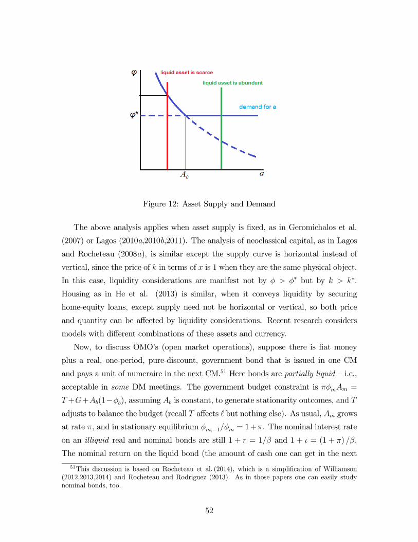
Figure 12: Asset Supply and Demand

The above analysis applies when asset supply is fixed, as in Geromichalos et al.

(2007) or Lagos (2010a,2010b,2011). The analysis of neoclassical capital, as in Lagos

and Rocheteau (2008a), is similar except the supply curve is horizontal instead of

vertical, since the price of in terms of is 1 when they are the same physical object.

In this case, liquidity considerations are manifest not by ∗ but by ∗.

Housing as in He et al. (2013) is similar, when it conveys liquidity by securing

home-equity loans, except supply need not be horizontal or vertical, so both price

and quantity can be affected by liquidity considerations. Recent research considers

models with different combinations of these assets and currency.

Now, to discuss OMO’s (open market operations), suppose there is fiat money

plus a real, one-period, pure-discount, government bond that is issued in one CM

and pays a unit of numeraire in the next CM.51 Here bonds are partially liquid — i.e.,

acceptable in some DM meetings. The government budget constraint is =

++(1−), assuming is constant, to generate stationarity outcomes, and

adjusts to balance the budget (recall affects but nothing else). As usual, grows

at rate , and in stationary equilibrium −1 = 1+. The nominal interest rate

on an illiquid real and nominal bonds are still 1 + = 1 and 1 + = (1 + ) .

The nominal return on the liquid bond (the amount of cash one can get in the next

51This discussion is based on Rocheteau et al. (2014), which is a simplification of Williamson

(2012,2013,2014) and Rocheteau and Rodriguez (2013). As in those papers one can easily study

nominal bonds, too.

52

CM by putting a dollar into real bonds in this CM) is , and generally differs from

. A straightforward application of the techniques used above lead to the FOC’s

−1 = 1( ) and −1 = 2( ).

In the DM, with probability a buyer meets a seller that accepts only , whence

he gets ; with probability a buyer meets one that accepts only , whence he

gets ; and with probability 2 a buyer meets one that accepts both, whence he gets

2. A realistic special case is = 0. Special cases of are ones where the assets are

perfect substitutes, = = 0, and where only cash is liquid, = 2 = 0. In

any case, we know that buyers must spend all their money in a type- meeting, and

may as well spend it all in a type-2 meeting since then both parties are indifferent

between combinations of and with the same value. Now, we know 2 ≤ , in

general, but there are still three possible cases: (i) = 2 = ; (ii) = 2;

and (iii) 2.

Consider case (i), and assume monetary equilibrium exists, which is valid at least

if is not too high. After some algebra, the Euler equations can be written

= () + 2(2) (36)

= () + 2(2) (37)

where ≡ (− ) (1 + ) is the spread between the returns on illiquid and liq-

uid bonds (as used in Wright 2010, Silveira and Wright 2010, and Rocheteau and

Rodriguez 2013). Just like is the return differential between illiquid bonds and cur-

rency, is the differential between illiquid and liquid bonds, and both measure the

cost of liquidity. It is also reminiscent of the “convenience yield” in Krishnamurthy

and Vissing-Jorgensen (2012) that they measure by the difference between yields on

government and corporate bonds.52

Notice standard accounting yields

=()− ()

1 + () + 2(2) (38)

This implies R 0 iff () R (). Hence, liquid bonds can have a negative

nominal return, 0, as is sometimes seen in reality (Wall Street Journal, Aug. 10,

52One may be tempted to say our model rationalizes their reduced-form specification with T-bills

in the utility function, although it’s not clear if that is desirable, any more than saying the models

presented above rationalize money in the utility function. The sine qua non of our approach is

modeling exchange explicitly, not deriving indirect utility functions from deeper primitives.

53

2012), even though we cannot have 0 for illiquid bonds. When 0, individuals

hold because it’s expected liquidity premium exceeds that on currency. Thus,

0 is impossible when = 0 or = ∗, and in particular = 2 = 0 implies

= . Importantly, 0 does not violate standard no-arbitrage conditions because

individuals cannot hold 0 — i.e., while anyone can issue a bond, they cannot

guarantee that it will circulate in the DM.53

Returning to the characterization of equilibrium in case (i), ( 2 ) solves

() = , () = , (2) = + , (36) and (37), while ( ) solves the usual

CM conditions. It is routine to derive the effects of inflation or the nominal interest

rate on illiquid bonds, and in particular 0, 0, = 0 and

2 0. Also, as long as 0 or 2 0, which means bonds are sometimes

accepted in the DM, higher raises the spread , or equivalently decreases and

increases , as agents try to shift from to . As regards an OMO, say selling

bonds for cash, since a one-time change in is as always neutral, this is the same

as simply increasing . Then 0 and 0 as long as 2 0, since

higher makes liquidity less scarce in type-2 meetings, so agents economize on ,

which hurts in type- meetings. Similarly, 0, and 2 0 as long as

0. If 2 0 and 0, by makes liquidity less scarce, higher reduces

and while increasing . Basically, an OMO reallocates liquidity between situations

where bonds are accepted and where they are not.54

Consider now a modification where agents learn what type of meeting they will

have in the DM before leaving the CM. Then without loss of generality, buyers who

will have a type- meeting carry only cash to the DM while those who will have a

type-2 meeting carry bonds and possibly cash. If is big then = 2 = ∗, no

one takes cash to meetings where bonds are accepted, and an OMO has no effect at

the margin. If is lower, we get ∈ (0 ) and a change in affects as well as

the allocation. If is too small then agents take some cash to type-2 meetings, and

= 2 ∗ despite = 0. This last outcome looks like a “liquidity trap” where

53He et al. (2008) or Sanches and Williamson (2010) also have liquid assets with negative nominal

returns if they are less susceptible to loss or theft than cash.54These results are for case (i). In cases (ii) and (iii) is determined as in a pure-currency

economy. The case that obtains depends on policy: if bonds are abundant, we get case (iii); if they

are less abundant, we get case (i) when is high and (ii) when is low. If 2 0 = = , so

bonds and money are perfect substitutes, an OMO is irrelevant because changes in are offset by

endogenous changes in , as in Wallace (1981,1983).

54

output is inefficiently low, the nominal rate on liquid bonds is 0, and OMO’s are

ineffectual. Again, these models are useful in trying to understand policy. And while

the preceding discussion concerned conventional monetary policy, swapping T-bills

for cash, one can obviously extend it to unconventional policy.

At this juncture we offer some general comments on the coexistence of money and

riskless, perfectly recognizable, nominal bonds with positive returns. Papers trying

to address this coexistence (or rate-of-return dominance) puzzle generally impose

some asymmetry between money and nominal bonds. An example is Aiyagari et

al. (1996), a second-generation model with money and two-period government bonds.

As in Li (1994,1995), Li and Wright (1998) or Aiyagari and Wallace (1997), there are

government agents that act like anyone else except: in meetings with private sellers,

they may either pay with money or issue a bond; in meetings with private buyers,

they may refuse to accept not-yet-matured bonds; and in any meeting they can turn

matured bonds into cash. Equilibria with valued money and interest-bearing bonds

exist because of asymmetry in the way government treats the assets. See also Zhu

and Wallace (2007), where the trading protocol gives a larger share of the surplus to

agents with more money.

Such asymmetries are adopted because of a belief that, under laissez faire, absent

exogenous assumptions that favor money there are no equilibria where it coexists with

default-free, interest-paying, nominal bearer bonds. Yet arguably there are historical

instances where such securities and money both circulated — a strong instance of the

rate-of-return-dominance puzzle. Lagos (2013a) addresses this in a version of Lagos-

Wright (2005) where currency consists of notes that are heterogeneous in extraneous

attributes called “moneyspots” to make a connection with sunspots; these can be any

payoff-irrelevant characteristic, like serial numbers. He shows this is all one needs

to get equilibria where money coexists with interest-bearing bonds. Heuristically, in

equilibrium the extraneous attributes are priced, so that different notes are valued

differently, supported purely by beliefs, and this allows money and nominal bonds to

coexist (see Lagos 2013a,b and Wallace 2013 for more discussion).

Moving from pure theory to more applied issue, Lagos (2008,2010b) shows how

liquidity helps us understand two of the best-known issues in finance, the risk-free-

rate and the equity-premium puzzles. There are two real assets, a one-period risk-free

55

government bond, and shares in a “tree” with random dividend , with prices and

. In a minor modification of the benchmark model, returns are in terms of a second

CM consumption good , which is numeraire, while is the price of , and CM utility

is ( ). Here both assets can be used in all DM transactions, 2 0 = = ,

but we consider 0 below. The Euler equations are

2£¡−1¢ −1

¤−1 = E 2 [ () ] [1 + 2 ()] (39)

2£¡−1¢ −1

¤−1 = E 2 [ () ] ( + ) [1 + 2 ()] (40)

using feasibility, = , where () solves 1 ( ) = 1.

Compared to our benchmark, now expected marginal utility 2 (·) at differentdates matters; compared to asset-pricing models following Mehra and Prescott (1985),

now liquidity matters. From (39)-(40) follow a pair of restrictions,

E(Ω − 1) = (41)

E[Ω( −)] = (42)

between the MRS, Ω ≡ 2 ( ) 2¡−1 −1

¢, and measured returns, ≡ 1−1

and ≡ ( + ) −1. For Mehra-Prescott, = = 0, and for standard prefer-

ences this is violated by data, where 0 and 0. By contrast, here

= −2E [Ω ()] (43)

= 2E [Ω () ( −)] (44)

From (43), 0 as long as 2 (+1) 0, which says the bond has liquidity

value in some state of the world. Hence, a liquidity-based model is always at least

qualitatively consistent with the risk-free-rate puzzle. Also, is the weighted average

return differential − across states. This is generally ambiguous in sign, but

suppose there is a high- and a low-growth state, and − is positive in the

latter and negative in the former. If the weight Ω () tends to be larger in the

low state, then 0. Hence, even without giving bonds an liquidity advantage

over equity, the model rationalizes the equity-premium puzzle. In a calibration with

( ) = () + 1− (1− ), the model is quantitatively consistent with both

puzzles for = 10, while standard calibrations of Mehra-Prescott need = 20.

Modest differences in acceptability matter a lot. If in 2% of DM trades buyers can

only use bonds, while in the remaining 98% they can use bonds or shares, then = 4

56

is enough to generate an equity premium of 7% — 10 times larger than Mehra-Prescott

with = 4. The broader point is that these models have a lot of potential for finan-

cial economics, and can have further implications for policy. In Lagos (2010a,2011),

currency and claims to a random aggregate endowment can both be used in the DM,

and in some states asset values are too low to get ∗. In such a model, monetary

policy can mitigate this by offsetting liquidity shortages. Even more generally, the

message is that liquidity considerations have important implications for the effects of

monetary policy on asset markets. This is no surprise. What we are suggesting is a

tractable GE framework that can be used to make this precise.55

11 Information and Liquidity

Going back to Law (1705), Jevons (1875) and others, one approach to understanding

the moneyness of assets appeals to informational frictions. Alchain (1977) iconoclas-

tically goes so far as to say “It is not the absence of a double coincidence of wants,

nor of the costs of searching out the market of potential buyers and sellers of various

goods, nor of record keeping, but the costliness of information about the attributes of

goods available for exchange that induces the use of money.” While all of the models

discussed above need some information frictions to make money essential, here we

have in mind private information about the quality of goods or assets.56

Williamson and Wright (1994) has no double coincidence problem, but barter

is hindered by agents trying to trade goods that are “lemons” — they are cheaper to

55In related work, Lagos (2010a) shows that a large class of money growth rules, as functions

of the state, implement = 0 and make asset prices independent of monetary considerations. But

one can alternatively target a constant 0, implying they depend on policy. In Lagos (2011),

deviations from an optimal policy make asset prices persistently deviate from “fundamental” values.

To support a constant the growth rate of the money supply must be low in states where real

asset values are low, introducing a negative relationship between and returns, with implications

for macro aggregates generally. Even if variations in output are exogenous, a positive correlation

between inflation and output emerges from targeting constant .56Recent studies of adverse selection in decentralized asset markets include Guerrieri et al. (2010),

Chiu and Koeppl (2011), Chang (2012) and Camargo and Lester (2013), but there assets play no role

in facilitating exchange. First-generation models with information frictions and assets playing this

role include Cuadras-Morató (1994), Williamson and Wright (1994), Li (1995,1998), Kim (1996),

Okumura (2006), and Lester et al. (2011). Second-generation models include Trejos (1997,1999),Velde et al. (1999), Burdett et al. (2001), Nosal and Wallace (2007) and Choi (2013). Models with

divisible assets include Berentsen and Rocheteau (2004), Shao (2009), Sanches and Williamson

(2011) and Lester et al. (2012). Related papers with private information about traders’ attributes

(e.g. preferences) include Faig and Jerez (2006), Ennis (2008) and Dong and Jiang (2010,2013).

57

produce but give less utility. Sometimes an agent recognizes quality before accepting a

good in trade, and sometimes not (it is match specific). Depending on parameters, it is

often the case that in equilibrium agents accept goods they do not recognize: Suppose

otherwise; then since agents who do recognize low-quality goods never accept them,

agents with “lemons” cannot trade; therefore no one produces “lemons” and hence

you can accept goods with impunity even if you cannot evaluate their quality before

trading. In this situation, equilibrium entails mixed strategies, where sellers produce

low quality, and buyers accept unrecognized goods, with positive probabilities. Fiat

currency can improve welfare, because in some monetary equilibria the incentive to

produce high quality goes up.

Moving to private information about asset quality, consider our benchmark econ-

omy with one-period-lived assets in fixed supply , with payoff ∈ , wherePr( = ) = and Pr( = ) = 1 − . Assume is common to all units of

the asset held by an agent, so it cannot be diversified, but it is independent across

agents — e.g., the payoff depends on local conditions specific to the holder. The asset

holder has private information about (as in Plantin 2009). Suppose the holder in

a meeting makes a take-it-or-leave-it offer. Using Cho and Kreps’ (1987) refinement,

Rocheteau (2011) shows the equilibrium is separating: holders of -type assets make

the full-information offer, () = min (∗) and = (), while holders

of -type assets make an offer satisfying

≥ () (45)

()− ≤ ()− () (46)

In particular, (46) says -type buyers have no incentive to offer ( ).

The least-cost separating offer satisfies (45)-(46) at equality, so = () ∈(0 ), while ∈ [0 ) solves () − () = () − ()Thus, -type

buyers retain a fraction of their holdings as a way to signal quality, and hence

(interpretable as over-collateralization, as in DeMarzo and Duffie 1999). When the

-type asset is a pure “lemon,” = 0, both and tend to 0.57 In contrast

57This is the case in Nosal and Wallace (2007), Shao (2009) and Hu (2013). The equilibrium,

however, would be defeated in the sense of Mailath et al. (1993). A perhaps more reasonable outcome

is the best pooling equilibrium from the viewpoint of a buyer with the -type asset, where solves

max()− st = (); this still implies is inefficiently low.

58

to models following Kiyotaki and Moore (1997) by assuming exogenous constraints,

here agents turn over all their assets in trade with probability 1 − , and a fraction

with probability , where depends on and . With a one-period-lived

asset, while ∗ = [ + (1− )] is the “fundamental” value, here we get

= ∗ +

½()()

() + − + (1− )()

¾

The liquidity premium − ∗ depends on − . As → , the premium

goes to (). As → 0, the asset becomes illiquid and → ∗. If the asset is

abundant, ≥ (∗), the liquidity premium is 0 even though = ∗. Thus,

can be inefficiently low even with abundant assets when they are imperfectly

recognizable, meaning other assets may also play an essential role. In Rocheteau

(2008), the second asset is fiat money. If it is perfectly recognizable then the same

logic applies: agents with -type assets make the complete-information offer while

those with -type assets make an offer that others do not want to imitate. When

→ 0, agents hold enough currency to buy ∗, and no one uses the asset in DM trade.

For 0 they do not hold enough currency to buy ∗, and spend it all plus a fraction

of their risky assets. Asset liquidity as measured by this fraction clearly depends on

monetary policy.58

Asset quality can also depend on hidden actions. One rendition allows agents to

produce assets of low quality, or that are outright worthless, as when through history

coins were clipped or notes counterfeited (Sargent and Velde 2003; Mihm 2007; Fung

and Shao 2011). Li et al. (2012) have a fixed supply of one-period-lived assets yielding

. At some fixed cost 0, agents can produce counterfeits that yield 0. Assume

counterfeits are confiscated by the government after each round of DM trade, so they

do not circulate across periods. Then with = 1, as above, the offer satisfies () ≤

58We emphasize the distinction between riskiness and asymmetric information here. Suppose the

asset is risky, but buyers and sellers have the same information when they meet (i.e., uncertainty is

resolved after trade). The asset then functions perfectly well as a medium of exchange, with actual

returns replaced by expected returns. However, suppose they are symmetrically informed but now

see the realization of before DM trade. Then risk is reflected in the previous CM price, with a

lower liquidity premium. Based on this reasoning, Andolfatto and Martin (2013) and Andolfatto et

al. (2014) consider an environment where the asset is risky and information about is available in

the DM, prior to trading, at zero cost. They show nondisclosure is generally desirable, because trade

based on expected dividends better smooths consumption. This result, however, can be overturned

if individuals are able to access hidden information.

59

and the IC is

−(− ∗)+ [()− ] ≥ −+ () (47)

where ∗ = . The LHS of (47) is the payoff to accumulating genuine assets,

the holding cost plus the DM surplus, while the RHS is the payoff to accumulating

counterfeits, cost plus the DM surplus.

Given = , in equilibrium, (47) can be rewritten as an upper bound on the

amount of asset that can be transferred,

≤

− ∗ + (48)

This endogenous upper bound increases with the cost of counterfeiting , while it

decreases with the cost of holding assets − ∗ and the frequency of DM trading

opportunities . If = 1, so there are no search or matching frictions in the DM,

(48) requires simply that the value of the asset is less than the cost of fraud . As

→ 0 the asset stops circulating. Notice also that an increase in the (endogenous)

price tightens the resalability constraint, which leads to pecuniary externalities with

non-trivial policy implications, as described in Li et al. (2012).

The CM asset price depending on parameters. If (48) binds and the asset

is illiquid at the margin and = ∗. If (48) does not bind the asset is perfectly liquid

and = ∗ + () with () = min (∗). There is an intermediate casewhere (48) binds, = , and = ∗ − + . In this case the liquidity

premium, −, increases with and decreases with . Notice the threatof fraud can affect asset prices even if fraud does not occur in equilibrium. The model

also explains why assets with identical yields can be priced differently. If the asset

subject to fraud is fiat money, as in Li and Rocheteau (2009), then (48) becomes

() ≤ (+ ), another case where acceptability is not exogenous. Other

extensions are Li and Rocheteau (2009) who have long-lived assets, Gomis-Porqueras

et al. (2014) who have two currencies and study exchange rates. See also Li et al.

(2012) and Williamson (2014), Li and Rocheteau (2011) and Shao (2013).59

59If we have multiple assets, each with cost of fraud and supply , then normalizing = 1 ∀,() = min

nP Ω (

∗)owhere Ω = 1 if 1 and Ω = 1 otherwise. Aggregate

liquidity is a weighted average of asset stocks, with weights depending asset characteristics, consistent

with a definition for the quantity of money suggested by Friedman and Schwartz (1970).

60

To this point we have assumed that sellers may be uninformed about the quality

of buyers’ assets. Lester et al. (2012) let sellers pay a cost to better recognize the

quality of an asset and hence endogenize the fraction of matches where it is accepted

(Kim 1996 and Berentsen and Rocheteau 2004 similarly let agents pay a cost to

better recognize the quality of goods). To simplify the analysis, Lester et al. (2012)

assume fraudulent assets are worthless and can be produced at no cost, = 0 and

= 0. This implies sellers only accept assets if they recognize them, and so we can

use standard bargaining theory — when sellers recognize assets there is no private

information; when they don’t the assets are not even on the bargaining table.

We now interpret as the probability of a single coincidence times the probability

that the seller can discern, and therefore accept, a buyer’s assets. The information

technology allows agents to choose at a cost () at the beginning of the DM, where

0 () 0 and 00 () 0 for 0, with 0(0) = 0 and 0() =∞ for some . The

decision of a seller to invest resources to become informed, so that he can accept assets

in the DM, is similar to a decision to enter market in the first place or the search

intensity decision discussed above. In order to give them some incentive to invest,

sellers must have some bargaining power, so we use Kalai’s solution with ∈ (0 1).The FOC is 0() = 0 [()− ()], where as always () = min (∗), with the dividend on genuine assets. This equates the marginal cost of becoming informed

to the expected benefit from being able to accept assets. As the marginal cost of

information decreases, and increase. If the asset is long lived, there are strategic

complementarities between agents’ holdings of liquid assets and their information

choice, creating the possibility of multiple steady-state equilibria.

Suppose there are two short-lived assets, both yielding . Asset 1 is perfectly

recognizable at no cost in a fraction of all meetings while asset 2 requires an ex

ante investment (2) to be acceptable in a fraction 2 of meetings. As a result, in

an endogenous fraction 2 of matches agents can pay with both assets, while in a

fraction 1 = −2 they can pay only with asset 1. The investment decision satisfies

0(2) = 0 [(2)− (2)]− [(1)− (1)] (49)

The RHS of (49) is the benefit to the seller from being informed, or the extra surplus

generated by having a payment capacity of (1 +2) instead of 1. Asset prices

are 1 = ∗ + 1(1) + 2(2) and 2 = ∗ + 2(2). If there is

61

an increase in the supply of recognizable assets 1, agents invest less in information,

and asset 2 becomes less liquid. As a result, 2 decreases. If the recognizable asset is

fiat money, then the acceptability of the other asset is affected by monetary policy.

At = 0, 1 = 2 = ∗ and agents stop investing in information, and asset 2 becomes

illiquid, reflecting the old idea that the use of money saves information costs.60

12 Generalized OTC Markets

Papers spurred by Duffie et al. (2005) maintain tractability by restricting ∈ 0 1;Lagos and Rocheteau (2009) relax this.61 For simplicity, suppose all trade goes

through dealers, as in Section 6 with 0 = . Let ∈ R+, and assume

() is the flow utility of an agent with preference type ∈ 0 . Each gets

a shock ∈ 0 at Poisson rate , withP

= . When with preference

contacts , they bargain over the that takes out of the meeting, and a payment

that includes ’s cost of the transaction ( − ) plus a fee (). The choice of

reduces to max0 (0)− 0, where

() ≡ ( + ) () +P

()

+ +

is the relevant arrival rate. The intermediation fee is

() = [ ()− ()− ( − )]

+ (50)

Equilibrium is given by the desired asset positions ( ), the fee (), the

that clears the interdealer market, and a distribution () satisfying the usual

conditions. Here we focus on implications for asset prices and measures of liquidity.

Let () = log , where 1 2 , and let =P

. Then

individual asset demand is

=( + ) ∞ +

+ + (51)

60Lester et al. (2012) and Zhang (2013) use versions of this model to study international issues.

Hu and Rocheteau (2014) use mechanism design, while Dong (2009), Nosal and Rocheteau (2011)

and Lotz and Zhang (2013) study money and credit. While this work focuses on information, other

aproaches include Zhu and Wallace (2007), Nosal and Rocheteau (2013) and Hu and Rocheteau

(2013). See also Kocherlakota (2003), Andolfatto (2011) and Jacquet and Tan (2012).61In spirit if not detail, the idea is to do what Section 7 does for monetary theory: extend second-

generation theory to a more general yet still tractable framework. The new model captures aspects

of illiquid markets like participants adjusting positions to reduce trading needs.

62

where ∞ = would be demand in a frictionless market, and = is demand

from with average valuation . In a frictional market, chooses holdings between

∞ and , with the weight assigned to ∞ increasing in . If can readjust more

frequently, they choose a position closer to the frictionless case.

Hence, frictions concentrate the asset distribution. As frictions decrease, → ∞and the distribution becomes more disperse, but aggregate demand is unchanged.

A message is that one should not expect to identify frictions by looking at prices

alone. Trade volume is

P | − | 2, lower than in a frictionless economy. It

increases with , capturing the idea that large volume characterizes liquid markets,

where can switch in and out of positions easily. Frictions have a direct plus indirect

effects on volume. If finds trading opportunities more frequently, the measure of

that can trade rises, but the measure that are mismatched falls. An increase in

shifts the distribution so that volume tends to increase. In contrast to Duffie et

al. (2005), where ∈ 0 1, now volume decreases with .62

Another measure of liquidity is the bid-ask spread or intermediation fee. In Duffie

et al. (2005), an increase in raises ’s value of search for alternative traders, so

spreads narrow. Now spreads still depend on , but also on the extent of mismatch

between asset positions and valuations. Hence, the relationship between the spread

and can be nonmonotone: under reasonable conditions, one can show the spread

vanishes as → 0 or as →∞. In liquid markets, has good outside options, andhence is small; in illiquid markets, trades very little, so ∞ is close to , and is

small. The model also predicts a distribution of transactions, with spreads increasing

in the size of a trade, as well as varying with ’s valuation.63 The model can also

be extended to allow heterogeneity across in terms of arrival rates or bargaining

power, and those with higher trade larger quantities at a lower cost per unit.

Trading delays are an integral feature of the microstructure in OTC markets.

The time it takes to execute a trade not only influences volume and spreads, but

is often used directly as a measure of liquidity. Lagos and Rocheteau (2007,2008b)

endogenize with entry by , and derive some new predictions, including a change

62Branzoli (2013) estimates a variant of this model using data from the municipal bond market.

He finds is sufficiently high to reduce trade volume by 65% to 70%.63The relationship between spread and trade size generally depends on details. Lester et al. (2013)

find with competitive search and a Leontief matching technology, costs decrease with the size of the

trade, in accordance with evidence from corporate bond markets.

63

in the equilibrium set due to the nonmonotonicity mentioned above. The model can

generate multiple equilibria: it may be illiquid because participation by is low

given a belief that will only trade small quantities; and it is rational for take

conservative positions given long trading delays. Tight spreads are correlated with

large volume and short delays across equilibria, and scarce liquidity can arise as a

self-fulfilling prophecy. Subsidizing entry can eliminate this multiplicity. Even when

equilibrium is unique, the model has novel predictions, like lower market power for

dealers promoting entry and reducing delays by increases trade size. Similarly, a

regulatory reform or a technological innovation that gives more direct access to

the market (e.g., Electronic Communication Networks) implies an increase in market

liquidity and intermediated trade.

The model also provides insights on welfare in illiquid markets. At least when

contact rates are exogenous, in Duffie et al. (2005) welfare is unaffected by , which

only affects transfers from to . When is not restricted to 0 1, equilibriumis inefficient unless = 0. Indeed, if captures any of the gains that gets from

adjusting his portfolio, economizes on intermediation fees by choosing closer to

, thus increasing mismatch. When is endogenous, the equilibrium is generically

inefficient, again related to Hosios (1990). Efficient entry requires equal the con-

tribution of dealers to the matching process, but efficiency along the intensive margin

requires = 0. As in monetary models, those two requirements are incompatible,

and the market is inefficient, although as in many other models, a competitive search

version can deliver efficiency (Lester et al. 2013).64

When = 0 , investors trade only with dealers who continuously manage

positions in a frictionless market. As mentioned earlier, some markets are well ap-

proximated by this, while others are better represented by 0, such as the Federal

Funds market, where commercial banks trade overnight loans typically without in-

termediation. Afonso and Lagos (2014a) model this explicitly. Banks have ∈ R+and trade bilaterally, and so there is a distribution (). Afonso and Lagos (2014b)

consider a special case with ∈ 0 1 2, where equilibrium is similar to some of the

monetary models above. More generally, Afonso and Lagos (2014a) show existence

and uniqueness, characterize the terms of trade, and address various positive and

64Branzoli (2013) finds that the most effective way to promote trading activity is the introduction

of weekly auctions where investors can trade bilaterally.

64

normative questions, including quantitative questions facing central banks.

In terms of other applications and extensions, Biais et al. (2014) give a reinterpre-

tation where agents have continuous access to the market, but learn their valuations

infrequently. They also provide a class of utility functions nesting Duffie et al. (2005)

and Lagos and Rocheteau (2009). Lagos and Rocheteau (2008) allow investors to

have both infrequent access to the market, where they are price-takers, and to deal-

ers, where they bargain. Pagnotta and Philippon (2012) use a similar model to study

marketplaces competing on speed. Melin (2012) has two types of assets traded in

different markets, one with search and one frictionless. Mattesini and Nosal (2013),

Geromichalos and Herrenbreuck (2013) and Lagos and Zhang (2013) integrate gener-

alized models of OTC markets with the monetary models in Section 7.

In particular, in Lagos and Zhang (2013) an asset called equity with dividend

is held by with time-varying idiosyncratic valuations. There are gains from trade

in from heterogeneous valuations, and participate in an OTC market like the DM

in our benchmark monetary model, but intermediated by , who again has access to

a frictionless interdealer market. In this market fiat money is essential as a medium

of exchange, and as usual some mechanism like bargaining determines the terms of

trade between and . The DM alternates with a frictionless CM where agents

rebalance portfolios. Equilibrium entails a cutoff preference type such that below

this who meets trades all his equity for cash and above this trades all his cash

for equity.65

When has all the bargaining power, he trades equity for cash at the price in

the interdealer market. If has all the bargaining power, trades at a price higher

(lower) than the interdealer market if wants to buy (sell) assets. This implies a

bid-ask spread determined by monetary policy, and details of the market structure,

such as the speed at which contacts or bargaining power. A nonmonetary equi-

librium always exists, and when is large it is the only equilibrium. In nonmonetary

equilibrium only holds equity, since there is no trade in the OTC market, and the

equity price is the expected discounted value of the dividend stream for the average

. Monetary equilibrium exists for lower . For not much larger than − 1, there65It would not be difficult to incorporate other assets or consider situations where agents obtain

money loans collateralized with assets. Basically, any of the extensions in the monetary models

discussed above can be incorporated.

65

is a unique stationary monetary equilibrium where holds all the equity overnight,

while holds it intraday. The asset price is higher than in nonmonetary equilibrium,

because OTC exchange props up the resale value of assets. As usual, the Friedman

rule implements the efficient allocation, and real asset prices decrease with be-

cause money is complementary with (used to purchase) . With entry by , Lagos

and Zhang (2013) generate sunspot equilibria with recurrent episodes that resemble

financial crises — when a sunspot shock hits, spreads spike, while volume, trading fre-

quency, market-making activity and asset prices collapse. As in many of the models

presented above, this is driven by the self-referential nature of liquidity.

Another area where New Monetarist models can provide useful and practical ad-

vice, somewhat related to the above-mentioned work on Fed Funds, concerns payment

and settlement systems in general. Central banks around the world oversee such sys-

tems, e.g., the Division of Reserve Bank Operations and Payment Systems oversees

the Federal Reserve Banks as providers of financial services to depository institutions

and fiscal agency services to the government. The cashless New Keynesian framework,

standard GE theory, or reduced form (e.g., CIA or MUF) models cannot address the

important issues faced by the regulators of these systems, where trade seems better

characterized as bilateral. Freeman (1996) is an early effort at formally modeling this

activity. Koeppl et al. (2008), Williamson and Wright (2010b, Sec. 5) and Nosal and

Rocheteau (2011,Ch. 9) present versions based on our benchmark model from Section

7. See McAndrews et al. (2011) for a survey of related work and a general discussion

of the issues.

13 Conclusion

The literature summarized in this survey helps us understand economic phenomena

at many levels and covers much territory, from rudimentary theories of commodity

money to fully-articulated quantitative macro systems to microstructure depictions

of Fed Funds trading. While they share some features, the models also vary a lot.

Some are relatively “clean” and have few hidden assumptions about the environment

or presumptions about behavior or institutions. This comes at a cost, and may entail

using primitive formulations. Other models are more sophisticated, and less “clean,”

because they are designed more for applications. This is not to say policy or empirical

66

work should use inferior theory. But there are tradeoffs, and finding the right balance

is part of the art of monetary economics. As with most art, what constitutes good

work is partly subjective, but technique matters, and it seems to us that much current

practice uses poor technique.66

It is poor technique to tell agents in a model to do something when there are

profitable deviations, as when they are assumed to make trades that are not in the

pairwise core because of an exogenous payment (e.g., CIA) constraint. We also think

it makes little sense to tell agents to take prices as given when prices are wrong due

to nominal rigidities. An artless claim would be that this is no different than impos-

ing restrictions on what they can do by specifying the environment in a particular

way. We disagree. Imposing frictions in the physical environment, like spatial sep-

aration, limited commitment or imperfect information, has all kinds of implications

for resource and incentive feasibility. The way to proceed is to lay out all of these

restrictions and draw out all their implications. This does not mean we necessarily

get the first best, since we must respect genuine frictions. But shortcuts like CIA

constraints are not the same as having genuine frictions in the environment; they are

impositions on behavior. We do not think the distinction is subtle.

We do not endorse the use of models with fiat currency in utility or production

functions. From a theoretical perspective, it means giving up on interesting and

challenging questions. From a policy perspective, it is all too obviously subject to

the Lucas critique. Of course, as with any specification, the appropriateness depends

on the issues at hand, but it is hard to imagine why anyone would prefer reduced-

form models. We can imagine hearing “this is the best we can do” — to which we

suggest “read the papers summarized above.” This does not mean assets in general

cannot appear in utility or production functions. Productive capital, housing, wine

and art belong there. Theories presented above take as primitives objects that may

give direct utility from consumption, like wine, or flow dividends, like art, and then

ask if and how they get used in the facilitation of exchange. Fiat money is special

because it provides no direct utility. But to study liquidity, when evaluating any

66Further discussion of reduced-form monetary theory follows below. As for the “cashless” New

Keynesian model, which attempts to avoid the charge of practicing poor monetary theory by ignoring

the issues, their downside is that they are unable to address virtually all the topics covered in this

essay, and that is perhaps a more serious indictment. Again, this is partly subjective, but it seems

incumbent upon us in this forum to profess our convictions.

67

asset, one should take into account its role in the exchange process. This necessitates

modeling the exchange process.

Since assets can show up in indirect utility or value functions, logically, it is

difficult to out-perform reduced-form models: whatever we adopt for primitives, the

same results (at least for a given set of observables) obtain if one starts with (·) andcalls that the utility of assets. The model in Section 7 is observationally equivalent

(for a given set of observables) to a MUF model with utility ()− + (), or a

CIA model with the constraint plugged in. But how does one know ex ante how to

specify (·)? Rather than guess, we derived

() = () + [ ()− ()] (52)

where key ingredients are and , capturing search and matching, and (), nesting

a general class of mechanisms. With heterogeneity due to either primitives, or to

histories, as in Molico (2006), the distribution () is another important ingredient,

because in models where agents trade with each other it determines trading partners,

and not just the slope of the budget line. With private information, also shows

up, looking like a pledgeability parameter in Kiyotaki-Moore (1997), except it is

endogenous, depending on policy, and can impact trade on intensive and extensive

margins (Lester et al. 2012; Li et al. 2012).

These key ingredients — , , , and — open up new avenues of theoretical

exploration, provide new insights into quantitative issues, and change our priors on

important policy questions. On inflation, in particular, the models presented above

incorporate a variety of effects: (i) inflation is a tax on real balances; (ii) some pricing

mechanisms, like bargaining, can compound this wedge; (iii) there are distortions on

the intensive and extensive margins, the latter revolving around participation deci-

sions, search intensity, congestion externalities and reservation trade decisions; (iv)

nominal rigidities, signal extraction problems, private information and related ele-

ments can be incorporated; and (v) there can be significant effects of the distribution

of liquidity and the distribution of prices. As compared to popular reduced-form

models, we learn a lot from considering ingredients they do not have. Other policy is-

sues that are affected by similar considerations include the desirability of low nominal

interest rates (they are typically good, but there are exceptions), the wisdom of trying

to reduce unemployment using expansionary policy (this can be counterproductive,

68

and even if feasible it can be undesirable), and the interpretation of sticky prices in

the data (they do not logically rationalize Keynesian theory or policy).

While the constraints in some of our models may “look like” CIA constraints, as

we said, they are really feasibility constraints. In some versions, like Kiyotaki-Wright

(1989), it is obvious that resource-feasibility restrictions imply one cannot turn over

something one does not have, and this is not a CIA constraint — indeed, the baseline

model does not even have cash. There are also incentive-feasibility restrictions that

need to be considered. In some models, you cannot issue an IOU if the other party

thinks you would renege because of commitment/enforcement limitations, and you

cannot easily use an asset for payment (or collateral) if they think it might be a

“lemon.” This does not come up in CIA models, where IOU’s and the use of other

assets are ruled out by fiat. The models here try to be explicit about the frictions

that make credit difficult, with Kocherlakota (1998) being a leading example, and

Kehoe-Livine (1993) or Kiyotaki-Moore (1997) also providing insight. Extensions of

our baseline model with multiple assets make it transparent that one does not need

to impose ad hoc restrictions on their use in transactions because this can be derived

endogenously. Which assets get used and how? A challenge is to look this (what

Helwig 1993 calls the modified Hahn problem) in the face, rather than evade it.

Based on this, we dispute the insinuation that search-and-bargaining models are

“the same as” CIA or MUF models (Camera and Chien 2013). Compared to (52),

they miss , which is especially important when endogenized via entry, intensity

or reservation decisions that are not invariant to interventions. The reduced-form

models we know also miss () by sticking to price taking behavior. Could one

add elements like , , (·) or (·) to those models? Sure. Then they would besearch-and-bargaining models. However, reduced-form theory still has fundamental

problems — e.g., it is not amenable to mechanism design, which is an important tool

for assessing the role of money and related institutions. But labels aside, an insight

that is obvious with the benefit of hindsight is that once one has such a specification

one does not need as hoc devices like CIA or MUF. A concrete example is Diamond

(1984), a version of Diamond (1982) with a CIA constraint. As one can learn from

Kiyotaki and Wright (1991,1993), in a very similar environment, once one thinks a

little more about specialization, which makes barter clumsy, as well as commitment

69

and information, which make credit untenable, one discovers there is a role for money

in this environment without a CIA constraint.

Although search per se is not critical, as we said several times, it can be conve-

nient for capturing the difficulty of barter and credit. Bargaining is also not crucial,

although it may be appropriate in some applications. Berentsen et al. (2011), e.g., in

accounting for the behavior of unemployment and inflation, argue that both search

and bargaining are important for qualitative and quantitative results. Bargaining

considerations can be also quantitatively relevant for understanding the effects of

monetary policy on welfare, employment and investment. But for other applica-

tions, other mechanisms are preferred, e.g., implementation of sticky-price theory

microfounded on Burdett-Judd (1982) pricing. Relatedly, Lagos (2010b) shows that

models with trading frictions help us understand issues in financial economics, like

the equity-premium or risk-free-rate puzzle, quantitatively. More generally, with rea-

sonable parameter values the models can generate equilibria that appear anomalous

from the vantage of standard asset-pricing theory, which we take to mean that finance

has something to learn from monetary economics (Rocheteau and Wright 2013). The

models also shed new light on optimal policy (Aruoba and Chugh 2008), banking

(Berentsen et al. 2011; Gu et al. 2013a), OTC markets (Duffie et al. 2011; Lagos

and Rocheteau 2009), and both conventional and unconventional monetary policy

(Williamson 2012,2014).

There is more research on related issues and models, but we have to stop some-

where. So here it is. Our hope is that readers will continue to search for developments

in the area, and that they have enjoyed — or at least survived — this guided tour.

70

Appendix on Notation (not necessarily for publication)

, , = arrival rate, discount rate, discount factor

= (utility of) dividend if 0 or storage cost if 0

= individual, aggregate asset holdings

, = single- and double-coincidence prob

, = cost and probability of entry a la Pissarides

= measure of type , = measure inventory

= monitoring probability

= fraction of monitored agents in CW

= trading strategy

= Υ () = best response correspondence

, = utility, cost of DM good

, = quantity in monetary, barter trades

, , , value fn for autarky, barter, credit and deviation

= value fn for ∈ 0 1 = bargaining power of agent with ∈ 0 1() = cost of — i.e., a general mechanism

= = arrive rate times bargaining power

, , = producer, middleman and consumer in RW

, = investor and dealer in DGP

= surplus in DGP

= probability of preference shock in DGP

() = asset dist’n

(), () = value fn for ∈ R+ in DM, CM, = (+ ) = price and value of

()− = CM utility

() = ()− () = DM surplus

, = DM quantity in money and in barter trades

, = = DM dollars and price

, = money growth (or inflation) and nominal interest rate

, , = gov’t consumption, transfers and other income in CM

= liquidity premium or Lagrange multiplier

, = factor prices for labor and capital

, = tax rates on labor and capital income

∆ = depreciation rate on

, Γ = DM utility fn, Γ1− (1− )

, = KM debt and haircut parameter

, = wedges on shares and bonds in Lagos JME

= 1 + = gross returns

= DM preference shock, ()

, 1− = probability that = , =

71

Appendix on Commodity Money

To explain the SS condition in Section 2, consider type 1 and pure strategies. If

1 has good 2, he can switch to good 3 only by trading with a 2 that has good 3

(since 3 never has good 3). For this, 1 has to meet 2 with good 3, which occurs

with probability 22, then trade, which occurs with probability 1 (since 2 always

wants good 2). And if 1 has good 3, he switches to good 2 only by acquiring good 1,

consuming and producing a new good 2 (he never switches from good 3 to 2 directly,

since if he preferred good 2 he would not trade it for good 3 in the first place). He

trades good 3 for good 1 either by trading with 3 that has good 1, which occurs with

probability 33, or with 2 that has good 1 but prefers good 3, which occurs with

probability 2 (1−2) (1− 2), but we can ignore that since either 2 = 1 or2 = 1.

Equating the measure of type 1 that switch from good 2 to good 3 and the measure

that switch back, we get (1).

case existence?

1 (1 1 1) (12 12 12) never

2 (1 1 0)¡√22√2− 1 1¢ maybe

3 (1 0 1)¡√2− 1 1√22¢ never

4 (1 0 0) (12 1 1) never

5 (0 1 1)¡1√22√2− 1¢ maybe

6 (0 1 0) (1 12 1) maybe

7 (0 0 1) (1 1 12) never

8 (0 0 0) (1 1 1) never

Table 1: Candidate Equilibria in the Commodity Money Model

Table 1 lists candidate equilibria, with existence results for the case = 13.

Consider case 1. After inserting , the BR conditions reduce to

∆1 ≥ 0, or 3 − 2 ≥ 6

∆2 ≥ 0, or 1 − 3 ≥ 6

∆3 ≥ 0, or 2 − 1 ≥ 6

Since these cannot all hold, this is never an equilibrium. In contrast, for case 2, the

BR conditions reduce to

∆1 ≥ 0, or 3 − 2 ≥ (1−√2)3

∆2 ≥ 0, or 1 − 3 ≥ 0∆3 ≤ 0, or 2 − 1 ≤ (1−

√22)3

For some parameters, these all hold and this is an equilibrium. The rest are similar.

72

References

G. Afonso and R. Lagos (2014) “Trade Dynamics in the Market for Federal Funds,”

NYU WP.

G. Afonso and R. Lagos (2014)“The Over-the-Counter Theory of the Fed Funds Market:

A Primer,” NYU WP.

S. Aiyagari and N. Wallace (1991) “Existence of Steady States with Positive

Consumption in the Kiyotaki-Wright Model,” RES 58, 901-16.

S. Aiyagari and N. Wallace (1992) “Fiat Money in the Kiyotaki-Wright Model,” ET 2,

447-64.

S. Aiyagari and N. Wallace (1997) “Government Transaction Policy, the Medium of

Exchange, and Welfare,” JET 74, 1-18.

S. Aiyagari, N. Wallace and R. Wright (1996) “Coexistence of Money and Interest-

Bearing Securities,” JME 37, 397-420.

A. Alchain (1977) “Why Money?” JMCB 9, 133-40.

L. Ales, F. Carapella, P. Maziero and W. Weber (2008) “A Model of Banknote

Discounts,” JET 142, 5-27.

C. Aliprantis, G. Camera and D. Puzzello (2006) “Matching and Anonymity,” ET 29,

415-32.

C. Aliprantis, G. Camera and D. Puzzello (2007) “Contagion Equilibria in a Monetary

Model,” Econometrica 75, 277-82.

C. Aliprantis, G. Camera and D. Puzzello (2007) “Anonymous Markets and Monetary

Trading,” JME 54, 1905-28.

N. Amendola and L. Ferraris (2013) “Money and Limited Enforcement in Multilateral

Exchange,” mimeo.

D. Andolfatto (2010) “Essential Interest-Bearing Money,” JET 145, 1495-507.

D. Andolfatto (2011) “A Note on the Societal Benefits of Illiquid Bonds,” CJE 44, 133-47.

D. Andolfatto (2013) “Incentive-Feasible Deflation,” JME 60, 383-90.

D. Andolfatto, A. Berentsen and C. Waller (2014) “Optimal Disclosure Policy and Undue

Diligence,” JET 149, 128-52.

D. Andolfatto and F. Martin (2013) “Information Disclosure and Exchange Media,” RED

16, 527-39.

L. Araujo (2004) “Social Norms and Money,” JME 51, 241-56.

L. Araujo and B. Camargo (2006) “Information, Learning and Stability of Fiat Money,”

JME 53, 1571-91.

L. Araujo and B. Camargo (2008) “Endogenous Supply of Fiat Money,” JET 142, 48-72.

L. Araujo, B. Camargo, R. Minetti and D. Puzzello (2012) “The Essentiality of Money in

Environments with Centralized Trade,” JME 59, 612-21.

L. Araujo and R. Minetti (2011) “On the Essentiality of Banks,” IER 52, 679-91.

L. Araujo and A. Shevchenko (2006) “Price Dispersion, Information and Learning,” JME

53, 1197-223.

S. Aruoba (2011) “Money, Search and Business Cycles,” IER 52, 935-59.

S. Aruoba and S. Chugh (2008) “Optimal Fiscal and Monetary Policy when Money is

Essential,” JET 145, 1618-47.

S. Aruoba, M. Davis and R. Wright (2014) “Homework in Monetary Economics,” mimeo.

73

S. Aruoba, G. Rocheteau and C. Waller (2007) “Bargaining and the Value of Money,”

JME 54, 2636-55.

S.Aruoba and F. Schorfheide (2011) “Sticky Prices vs Monetary Frictions: An Estimation

of Policy Tradeoffs,” AJMacro 3(1), 60-90.

S. Aruoba, C. Waller and R. Wright (2011) “Money and Capital,” JME 58, 98-116.

S. Aruoba and R. Wright (2003) “Search, Money and Capital,” JMCB 35, 1085-05.

C. Azariadis (1993) Intertemporal Macroeconomics. Oxford: Blackwell.

M. Bailey (1956) “The Welfare Cost of Inflationary Finance,” JPE 64, 93-11.

E. Basçı (1999) “Learning by Imitation,” JEDC 23, 1569-85.

R. Benabou (1988) “Search, Price Setting and Inflation.” RES 55, 353-76.

R. Benabou (1992) “Inflation and Efficiency in Search Markets,” RES 59, 299-329.

V. Bencivenga and G. Camera (2011) “Banks, Liquidity Insurance, and Interest on

Reserves in a Matching Model,” JMCB 43, 449-76.

A. Berentsen (2002) “On the Distribution of Money Holdings in a Random-Matching

Model,” IER 43, 945-54.

A. Berentsen, G. Camera and C. Waller (2005) “The Distribution Of Money Balances and

the Nonneutrality Of Money,” IER 46, 465-87.

A. Berentsen, G. Camera and C. Waller (2007) “Money, Credit, and Banking,” JET 135,

171-95.

A. Berentsen, G. Menzio and R. Wright (2011) “Inflation and Unemployment in the Long

Run,” AER 101, 371-98.

A. Berentsen, M. Molico and R. Wright (2002) “Indivisibilities, Lotteries and Monetary

Exchange,” JET 107, 70-94.

A. Berentsen and C. Monnet (2008) “Monetary Policy in a Channel System,” JME 55,

1067-08.

A. Berentsen and G. Rocheteau (2002) “On the Efficiency of Monetary Exchange: How

Divisibility of Money Matters,” JME 49, 1621-49.

A. Berentsen and G. Rocheteau (2003) “"Money and the Gains from Trade,” IER 44,

263-97.

A. Berentsen and G. Rocheteau (2003) “On the Friedman Rule in Search Models with

Divisible Money,” BEJ Macro 3(1), 1-21.

A. Berentsen and G. Rocheteau (2004) “Money and Information,” RES 71, 915-44.

A. Berentsen, G. Rocheteau and S. Shi (2007) “Friedman Meets Hosios: Efficiency in

Search Models of Money,” EJ 117, 174-95.

A. Berentsen M. Rojas Breu and S. Shi (2012) “Liquidity, Innovation and Growth,” JME

59, 721-37.

A. Berentsen and C. Waller (2011) “Outside versus Inside Bonds: A Modigliani-Miller

Type Result for Liquidity Constrained Cconomies,” JET 146, 1852-87.

A. Berentsen and C. Waller (2011) “Price-Level Targeting and Stabilization Policy,”

JMCB 43, 559-80.

Z Bethune, M. Choi and R. Wright (2014) “Semi-Directed Search,” mimeo.

Z. Bethune, G. Rocheteau and P. Rupert (2012) “Unemployment and Household

Unsecured Debt,” mimeo.

B. Biais, J. Hombert and P. Weill (2014) “Equilibrium Pricing and Trading Volume under

Preference Uncertainty,” RES, in press.

74

K. Binmore, A. Rubinstein and A. Wolinsky (1986) “The Nash Bargaining Solution in

Economic Modelling,” Rand 17, 176-88.

P. Boel and G. Camera (2006) ‘Efficient Monetary Allocations and the Illiquidity of

Bonds,” JME 53, 1693-715.

P. Boel and G. Camera (2009) “Financial Sophistication and the Distribution of the

Welfare Cost of Inflation,” JME 56, 968-78.

P. Boel and G. Camera (2011) “The Welfare Cost of Inflation in OECD Countries,” MD

15, 217-51.

M. Boldrin, N. Kiyotaki and R. Wright (1993) “A Dynamic Equilibrium Model of Search,

Production and Exchange,” JEDC 17, 723-58.

N. Branzoli (2013) “The Effect of Intermediaries’ Market Power in Decentralized Asset

Markets,” mimeo.

P. Brown (1996) “Experimental Evidence on Money as a Medium of Exchange,” JEDC

20, 583-600.

K. Burdett, M. Coles, N. Kiyotaki and R. Wright (1995) “Buyers and Sellers: Should I

Stay or Should I Go?" AER Papers & Proceedings 85, 281-86.

K. Burdett and K. Judd (1983) “Equilibrium Price Dispersion,” Econometrica 51, 955-69.

K. Burdett and G. Menzio (2014) “The (Q,s,S) Pricing Rule,” mimeo.

K. Burdett, G. Menzio and R. Wright (2014) “A Simple Model of Nominal Price

Dispersion and Rigidity,” mimeo.

K. Burdett, A. Trejos and R. Wright (2001) “Cigarette Money,” JET 99, 117-42.

B. Camargo and B. Lester (2013) “Trading Dynamics in Decentralized Markets with

Adverse Selection,” mimeo.

G. Camera (2001) “Search, Dealers, and the Terms of Trade,” RED 4, 680-94.

G. Camera and Y. Chien (2013) “Modeling Monetary Economies: An Equivalence

Result,” mimeo.

G. Camera and D. Corbae (1999) “Money and Price Dispersion,” IER 40, 985-1008.

G. Camera and Y. Li (2008) “Another Example of a Credit System that Coexists with

Money,” JMCB 40, 1295-308.

G. Camera, R. Reed and C. Waller (2003) “Jack of All Trades or a Master of One:

Specialization, Trade, and Money,” IER 44, 1275-94.

G. Camera, B. Craig and C. Waller (2004) “Currency Competition in a Fundamental

Model of Money,” JIE 64, 521-44.

R. Cavalcanti (2004) “A Monetary Mechanism for Sharing Capital: Diamond and Dybvig

Meet Kiyotari and Wright,” ET 24, 769-88.

R. Cavalcanti, A. Erosa and T. Temzilides (1999) “Private Money and Reserve

Management in a Random-Matching Model,” JPE 107, 929-45.

R. Cavalcanti, A. Erosa and T. Temzilides (2005) “Liquidity, Money Creation and

Destruction and the Returns to Banking,” IER 46, 675-706.

R. Cavalcanti and N. Wallace (1999). “A Model of Private Banknote Issue,” RED 2,

104-36.

R. Cavalcanti and N. Wallace (1999). “Inside and Outside Money as Alternative Media

of Exchange,” JMCB 31, 443-57.

B. Chang (2012) “Adverse Selection and Liquidity Distortion,” mimeo.

75

V. Chari, L. Christiano and P. Kehoe (1991) “Optimal Fiscal and Monetary Policy: Some

Recent Results," JMCB 23, 519-39.

J. Chiu and T. Koeppl (2011) “Trading Dynamics with Adverse Selection,” mimeo.

J. Chiu and C. Meh (2011) “Financial Intermediation, Liquidity and Inflation,” MD 15,

83-118.

J. Chiu, C. Meh and R. Wright (2013) “Innovation and Growth with Financial, and

Other, Frictions,” mimeo.

J. Chiu and M. Molico (2010) “Endogenously Segmented Markets in a Search Theoretic

Model of Monetary Exchange,” JME 57, 428-38.

J. Chiu and M. Molico (2011) “Uncertainty, Inflation, and Welfare,” JMCB 43, 487-512.

I. Cho and D. Kreps (1987) ‘Signaling Games and Stable Equilibria,” QJE 102, 179-221.

M. Choi (2013) “Asset Markets with Adverse Selection and Memory Loss,” mimeo.

R. Clarida, J. Gali and M. Gertler (1999) “The Science of Monetary Policy: A New

Keynesian Perspective,” JEL 37, 1661-707.

R. Clower (1970) “Is There an Optimal Money Supply?” JF Papers and Proceedings 25,

425-33.

H. Cole and N. Kocherlakota (1998) “Zero Nominal Interest Rates: Why They’re Good

and How to Get Them,” FRB Minneapolis QR 22, 2-10.

M. Coles (1999) “Turnover Externalities with Marketplace Trading,” IER 40, 851-68.

M. Coles and R. Wright (1998) “A Dynamic Model of Search, Bargaining, and Money,”

JET 78, 32-54.

T. Cooley and G. Hansen (1989) “The Inflation Tax in a Real Business Cycle Model,”

AER 79, 733-48.

D. Corbae and J. Ritter (2004) “Decentralized Credit and Monetary Exchange without

Public Record Keeping,” ET 24, 933-51.

D. Corbae, T. Temzilides and R. Wright (2002) “Matching and Money,” AER Papers &

Proceedings 92, 67-71.

D. Corbae, T. Temzilides and R. Wright (2003) “Directed Matching and Monetary

Exchange,” Econometrica 71, 731-56.

I. Correia, P. Teles and J. Nicolini (2008) “Optimal Fiscal and Monetary Policy:

Equivalence Results,” JPE 116, 141-70

B. Craig and G. Rocheteau (2008) “Inflation and Welfare: A Search Approach,” JMCB

40, 89-119.

B. Craig and G. Rocheteau (2008) “State-Dependent Pricing, Inflation, and Welfare in

Search Economies,” EER 52, 441-68.

B. Craig and C. Waller (2004) “Currency Portfolios and Currency Exchange in a Search

Economy,” JME 51,671-89.

X. Cuadras-Morato (1994) “Commodity Money in the Presence of Goods of

Heterogeneous Quality,” ET 4, 579-91.

X. Cuadras-Morato (1997) “Can Ice Cream be Money?: Perishable Medium of

Exchange,” J Economics 66, 103-25.

E. Curtis and C. Waller (2000) “A Search Theoretic Model of Legal and Illegal

Currency,” JME 45, 155-84.

E. Curtis and C. Waller (2003) “Currency Restrictions, Government Transaction Policies

and Currency Exchange,” ET 21, 19-42.

76

E. Curtis and R. Wright (2004) “Price Setting, Price Dispersion, and the Value of Money;

or, The Law of Two Prices,” JME 51, 1599-621.

B. Cynamon, D. Dutkowsky and B. Jones (2006) “Redefining the Monetary Agggregates:

A Clean Sweep,” Eastern Econ J 32, 661-72.

G. Debreu (1959) Theory of Value: An Axiomatic Analysis of Economic Equilibrium.

Yale University Press.

P. DeMarzo and D. Duffie (1999) “A Liquidity-Based Model of Security Design,”

Econometrica 67, 65-99.

A. Deviatov (2006) “Money Creation in a Random Matching Model,” BEJ Topics in

Macro 6(3), 1-20.

A. Deviatov and N. Wallace (2009) “A Model in which Monetary Policy is about Money,”

JME 56, 283-88.

A. Deviatov and N. Wallace (2014) “Optimal Inflation in a Model of Inside Money,”

RED, in press.

D. Diamond (1984) “Financial Intermediation and Delegated Monitoring,” RES 51,

393-414.

D. Diamond and P. Dybvig (1983) “Bank Runs, Deposit Insurance, and Liquidity,” JPE

91, 401-19.

P. Diamond (1982) “Aggregate Demand Management in Search Equilibrium,” JPE 90,

881-94.

P. Diamond (1984) “Money in Search Equilibrium,” Econometrica 52, 1-20.

P. Diamond (1993) “Search, Sticky Prices and Inflation,” RES 60, 53-68.

P. Diamond and D. Fudenberg (1989) “Rational Expectations Business Cycles in Search

Equilibrium,” JPE 97, 606-19.

M. Dong (2010) “Inflation and Variety,” IER 51, 401-20.

M. Dong (2011) “Inflation and Unemployment in Competitive Search Equilibrium,” MD

15, 252-68.

M. Dong J. Jiang (2010) “One or Two Monies?" JME 57, 439-450.

M. Dong and J. Jiang (2013) “Money and Price Posting under Private Information,”

JET, in press.

M. Dong and X. Xiao (2013) “Liquidity, Monetary Policy and Unemployment,” mimeo.

S. Dressler (2011) “Money Holdings, Inflation, and Welfare in a Competitive Market,”

IER 52, 407-23.

S. Dressler (2011) “A Long-run, Short-run and Politico-economic Analysis of the Welfare

Costs of Inflation,” mimeo.

D. Duffie, N. Gârleanu and L. Pederson (2005) “Over-the-Counter Markets,”

Econometrica 73, 1815-47.

D. Duffie, N. Gârleanu and L. Pederson (2007) “Valuation in Over-the-Counter Markets,”

RFS 20, 1865-1900.

J. Duffy (2001) “Learning to Speculate: Experiments with Artificial and Real Agents,”

JEDC 25, 295-319.

J. Duffy and J. Ochs (1999) “Emergence of Money as a Medium of Exchange: An

Experimental Study,” AER 847-77.

J. Duffy and J. Ochs (2002) “Intrinsically Worthless Objects as Media of Exchange:

Experimental Evidence,” IER 43, 637-73.

77

J. Duffy and D. Puzzello (2013) “Gift Exchange versus Monetary Exchange: Theory and

Evidence,” AER, in press.

R. Dutta (2012) “Bargaining with Revoking Costs,” GEB 74, 144-53.

R. Dutu (2006) “The Costs of Inflation in Australia and New Zealand,” NZ Econ Papers

40, 127-14.

R. Dutu and S. Huangfu and B. Julien (2011) “Contingent Prices And Money,” IER 52,

1291-308.

R. Dutu, B. Julien and I. King (2012) “On the Welfare Gains of Price Dispersion,” JMCB

44, 757-86.

M. Engineer and S. Shi (1998) “Asymmetry, Imperfectly Transferable Utility, and the

Role of Fiat Money in Improving Terms of Trade,” JME 41, 153-83.

M. Engineer and S. Shi (2001) “Bargains, Barter and Money,” RED 4, 188-209.

H. Ennis (2001) “On Random Matching, Monetary Equilibria, and Sunspots,” MD 5,

132-42.

H. Ennis (2008) “Search, Money, and Inflation under Private Information,” JET 138,

101-31.

H. Ennis (2009) “Avoiding the Inflation Tax,” IER 50, 607-62.

M. Faig (2008) “Endogenous Buyer—Seller Choice and Divisible Money in Search

Equilibrium,” JET 141, 184-99.

M. Faig and S. Huangfu (2007) “Competitive-Search Equilibrium in Monetary

Economies,” JET 136, 709-18.

M. Faig and B. Jerez (2005) “A Theory of Commerce,” JET 122, 60-99.

M. Faig and B. Jerez (2006) “Inflation, Prices, and Information in Competitive Search,”

BEJ Macro 6.

M. Faig and Z. Li (2009) “The Welfare Costs of Expected and Unexpected Inflation,”

JME 56, 1004-13.

L. Ferraris and M. Watanabe (2008) “Collateral Secured Loans in a Monetary Economy,”

JET 143, 405-24.

L. Ferraris and M. Watanabe (2011) “Collateral Fluctuations in a Monetary Economy,”

JET 146, 1915-40.

L. Ferraris and M. Watanabe (2012) “Liquidity Constraints in a Monetary Economy,”

IER 53, 255-77.

M. Friedman (1960) A Program for Monetary Stability, Fordham University Press, New

York.

S. Freeman (1996) “The Payments System, Liquidity, and Rediscounting,” AER 86,

1126-38.

M. Friedman (1968) “The Role of Monetary Policy,” AER 58, 1-17.

M. Friedman (1969) The Optimum Quantity of Money and Other Essays. Aldine.

M. Friedman (1977) “Inflation and Unemployment,” JPE 85, 451-72.

M. Friedman (1992) Money Mischief: Episodes in Monetary History. Harcourt.

B. Fung and E. Shao (2011) “Modelling the Counterfeiting of Bank Notes: A Literature

Review,” Bank of Canada Rev, Autumn, 29-35.

D. Gale and L. Shapley (1962) “College Admissions and the Stability of Marriage,” Amer.

Math. Monthly 69, 9-15.

78

M. Galenianos and P. Kircher (2008) “A Model of Money with Multilateral Matching,”

JME 55, 1054-66.

A. Gavazza (2011) “The Role of Trading Frictions in Real Asset Markets,” AER 101,

1106-43.

A. Geromichalos and L. Herrenbreuck (2013) “Monetary Policy, Asset Prices, and

Liquidity in Over-the-Counter Markets,” mimeo.

A. Geromichalos, J. Licari and J. Lledo (2007) “Asset Prices and Monetary Policy,” RED

10, 761-79.

A. Geromichalos and I Simonovska (2014) “Asset Liquidity and International Portfolio

Choice,” JET, in press.

A. Geromichalos, L. Herrenbrueck and K, Salyer (2013) “A Search-Theoretic Model of the

Term Premium," mimeo.

M. Gertler and N. Kiyotaki (2010) “Financial Intermediation and Credit Policy in

Business Cycle Analysis,” Handbook of Monetary Economics, vol. 2, B. Friedman and M.

Woodford, eds. North-Holland, Amsterdam.

V. Guerrieri and G. Lorenzoni (2009) “Liquidity and Trading Dynamics,” Econometrica

77, 1751-90.

P. Gomis-Porqueras, B. Julien and C. Wang (2013) “Optimal Monetary and Fiscal

Policies in a Search-theoretic Model of Money and Unemployment,” MD 17(6), 1330-54.

P. Gomis-Porqueras and A. Peralta-Alva (2010) “Optimal Monetary and Fiscal Policies in

a Search Theoretic Model of Monetary Exchange,” EER 54, 331-44.

P. Gomis-Porqueras, T. Kam and C. Waller (2014) “Breaking the Curse of Kareken and

Wallace,” mimeo.

E. Green and W. Weber (1996) “Will the New $100 Bill Decrease Counterfeiting?” FRB

Minneapolis QR.

E. Green and R. Zhou (1998) “A Rudimentary Random-Matching Model with Divisible

Money and Prices,” JET 81, 252-71.

E. Green and R. Zhou (2002) “Dynamic Monetary Equilibrium in a Random Matching

Economy,” Econometrica 70, 929-69.

C. Gu, F. Mattesini, C. Monnet and R. Wright (2013) “Banking: A New Monetarist

Approach,” RES 80, 636-62.

C. Gu, F. Mattesini, C. Monnet and R. Wright (2013) “Endogenous Credit Cycles,” JPE

121, 940-65.

C. Gu, F. Mattesini and R. Wright (2014) “Money and Credit Redux,” mimeo.

V. Guerrieri R. Shimer and R. Wright (2010) “Adverse Selection in Competitive Search

Equilibrium,” Econometrica 78, 1823-62.

F. Hahn (1965) “On Some Problems of Proving the Existence of an Equilibrium in a

Monetary Economy,” in The Theory of Interest Rates, F. Hahn and F. Brechling, eds.

F. Hahn (1973) “On the Foundations of Monetary Theory,” in Modern Economics, M.

Parkin and A. Nobay, eds., New York: Barnes & Noble

F. Hahn (1987) “The Foundations of Monetary Theory,” in M. de Cecco and J. Fitoussi,

eds., Monetary Theory and Economic Institutions, London: MacMillan.

G. Hansen (1985) “Indivisible Labor and the Business Cycle,” JME 16, 309-37.

F. Hayashi and A. Matsui (1996) “A Model of Fiat Money and Barter,” JET 68, 111-32.

79

A. Haug and I. King (2014) “In the Long Run, US Unemployment Follows Inflation Like

a Faithful Dog,” J Macro, in press.

P. He, L. Huang and R. Wright (2005) “Money and Banking in Search Equilibrium,” IER

46, 637-70.

P. He, L. Huang and R. Wright (2008) “Money, Banking and Monetary Policy,” JME 55,

1013-24.

C. He, R. Wright and Y. Zhu (2013) “Housing and Liquidity,” mimeo.

A. Head and A. Kumar (2005) “Price Dispersion, Inflation, and Welfare,” IER 46, 533-72.

A. Head, A. Kumar and B. Lapham (2010) “Market Power, Price Adjustment, and

Inflation,” IER 51, 73-98.

A. Head, L. Liu, G. Menzio and R. Wright (2012) “Sticky Prices: A New Monetarist

Approach,” JEEA 10, 939-73.

A. Head and S Shi (2003) “A Fundamental Theory of Exchange Rates and Direct

Currency Trades,” JME 50, 1555-91.

M. Hellwig (1993) “The Challenge of Monetary Theory,” EER 37, 215-42.

J. Hicks (1935) “A Suggestion for Simplifying the Theory of Money,” Economica 2, 1-19.

T. Hogan and W. Luther (2014) “Endogenous Matching and Money with Random

Consumption Preferences,” mineo.

P. Howitt (2005) “Beyond Search: Fiat Money in Organized Exchange,” IER 46, 405-29.

A. Hosios (1990) “On the Efficiency of Matching and Related Models of Search and

Unemployment,” RES 57, 279-98.

T. Hu (2013) “Imperfect Recognizability and Coexistence of Money and Higher-Return

Assets,” ET 53, 111-38.

T. Hu and G. Rocheteau (2013) “On the Coexistence of Money and Higher Return

Assets,” JET 148, 2520-60.

T. Hu and G. Rocheteau (2014) “Monetary Policy and Asset Prices: A Mechanism

Design Approach,” mimeo.

T. Hu, J. Kennan and N. Wallace (2009) “Coalition-Proof Trade and the Friedman Rule

in the Lagos-Wright Model,” JPE 117, 116-37.

T. Hu, C. Zhang and A. Komai (2014) “Responding to the Inflation Tax,” mimeo.

S. Huangfu (2009) “Competitive Search Equilibrium with Private Information on

Monetary Shocks,” BEJ Macro 9(1), 1-27.

K. Iwai (1996) “The Bootstrap Theory of Money: A Search-Theoretic Foundation of

Monetary Economics,” Structural Change & Econ Dynamics 7, 451-77.

N. Jacquet and S. Tan (2011) “Money, Bargaining, and Risk Sharing,” JMCB 43, 419-42.

N. Jacquet and S. Tan (2012) “Money and Asset Prices with Uninsurable Risks,” JME

59, 784-97.

K. Jean, S. Rabinovich and R. Wright (2010) “On the Multiplicity of Monetary Equilibria

Green-Zhou Meets Lagos-Wright,” JET 145, 392-401.

W. Jevons (1875) Money and the Mechanism of Exchange. Appleton.

G. Jin and T. Zhu (2014) “Non-Neutrality of Money : Hume Revisited,” mimeo.

A. Johri (1999) “Search, Money, and Prices,” IER 40, 439-54.

B. Julien, J. Kennes and I. King (2008) “Bidding For Money,” JET 142, 196-217.

R. Jones (1976) “The Origin and Development of Media of Exchange,” JPE 84, 757-75.

C. Kahn, J. McAndrews and W. Roberds (2005) “Money Is Privacy,” IER 46, 377-99.

80

C. Kahn and W. Roberds (2008) “Credit and Identity Theft,” JME 55, 251-64.

E. Kalai (1977) “Proportional Solutions to Bargaining Situations: Interpersonal Utility

Comparisons,” Econometrica 45, 1623-30.

K. Kamiya, N. Morishita and T. Shimizu (2005) “On the Existence of Single-Price

Equilibria in a Matching Model with Divisible Money and Production Cost,” IJET 1,

219-31.

K. Kamiya and T. Sato (2004) “Equilibrium Price Dispersion in a Matching Model with

Divisible Money,” IER 45, 413-30.

K. Kamiya and T. Shimizu (2006) “Real indeterminacy of stationary equilibria in

matching models with divisible money,” J Math Econ 42, 594-617.

K. Kamiya and T. Shimizu (2007) “On the Role of Tax Subsidy Schemes in Money

Search Models,” IER 48, 575-606.

K. Kamiya and T. Shimizu (2007) “Existence of Equilibria in Matching Models of

Money: A New Technique,” Econ Theory 32, 447-60.

J. Kareken and N. Wallace (1980) “Introduction,” in Models of Monetary Economies, J.

Kareken and N. Wallace, eds. FRB Minneapolis.

B. Katzman, J. Kennan N. Wallace (2003) “Output and price level effects of monetary

uncertainty in a matching model,” JET 108, 217-55.

T. Kehoe, N. Kiyotaki and R. Wright (1993) “More on Money as a Medium of

Exchange,” ET 3, 297-314.

T. Kehoe and D. Levine (1993) “Debt-Constrained Asset Markets,” RES 60, 865-88.

J. Keynes (1936) The General Theory, London: Palgrave-Macmillan.

J. Keynes (1924) A Tract on Monetary Reform, Amherst, NY: Prometheus.

Y. Kim (1996) “Money, Barter, and Costly Information Acquisition,” JME 37, 119-42.

N. Kiyotaki and J. Moore (1997) “Credit Cycles,” JPE 105, 211-48.

N. Kiyotaki and J. Moore (2001) “Evil is the Root of All Money,” mimeo.

N. Kiyotaki and J. Moore (2005) “Liquidity and Asset Prices,” IER 46, 317-49.

N. Kiyotaki and R. Wright (1989) “On Money as a Medium of Exchange,” JPE 97,

927-54.

N. Kiyotaki and R. Wright (1991) “A Contribution to the Pure Theory of Money,” JET

53, 215-35.

N. Kiyotaki and R. Wright (1993) “A Search-Theoretic Approach to Monetary

Economics,”AER 83, 63-77.

P. Klenow and O. Kryvtsov (2008) “State-Dependent or Time-Dependent Pricing: Does it

Matter for Recent U.S. Inflation?” QJE 123, 863-904.

N. Kocherlakota (1998) “Money is Memory,” JET 81, 232-51.

N. Kocherlakota (2003) “Societal Benefits of Illiquid Bonds,” JET 108, 179-93.

N. Kocherlakota and N. Wallace (1998) “Incomplete Record-Keeping and Optimal

Payment Arrangements,” JET 81, 272-89.

T. Koeppl, C. Monnet and T. Temzilides (2008) “A Dynamic Model of Settlement,” JET

142, 233-46.

A. Krishnamurthy and A. Vissing-Jorgensen (2012) “The Aggregate Demand for Treasury

Debt,” JPE 120, 233-67.

A. Kumar (2008) “Inflation and the Dispersion of Real Wages,” IER 49, 377-99.

81

R. Lagos (2008) “Research Agenda: Liquidity and the Search Theory of Money,” SED

Newsletter.

R. Lagos (2010) “Some Results on the Optimality and Implementation of the Friedman

Rule in the Search Theory of Money,” JET 145, 1508-24.

R. Lagos (2010)“Asset Prices and Liquidity in an Exchange Economy,” JME 57, 913-30.

R. Lagos (2011) “Asset Prices, Liquidity, and Monetary Policy in an Exchange Economy,”

JMCB 43, 521-52.

R. Lagos (2013) “Moneyspots,” JPE 121, 127-85.

R. Lagos (2013) “Moneyspots and Coexistence in the Pure Theory of Money: A Reply

to Neil Wallace,” JPE 121, 796-801.

R. Lagos and G. Rocheteau (2005) “Inflation, Output, and Welfare,” IER 46, 495-522.

R. Lagos and G. Rocheteau (2007) “Search in Asset Markets: Market Structure,

Liquidity, and Welfare,” AER Papers & Proceedings 97, 198-202.

R. Lagos and G. Rocheteau (2008) “Money and Capital as Competing Media of

Exchange,” JET 142, 247-258.

R. Lagos and G. Rocheteau (2008) “Liquidity in Asset Markets with Search Frictions,”

FRB Cleveland WP 08-04.

R. Lagos and G. Rocheteau (2009) “Liquidity in Asset Markets with Search Frictions,”

Econometrica 77, 403-26.

R. Lagos, G. Rocheteau and P. Weill (2011) “Crises and Liquidity in Over-the-Counter

Markets,” JET 146, 2169-205.

R. Lagos and R. Wright (2003) “Dynamics, Cycles and Sunspot Equilibria in ‘Genuinely

Dynamic, Fundamentally Disaggregative’ Models of Money,” JET 109, 156-71.

R. Lagos and R. Wright (2005) “A Unified Framework for Monetary Theory and Policy

Analysis,” JEP 113, 463-44.

R. Lagos and S. Zhang (2013) “A Model of Monetary Exchange in Over-the-Counter

Markets,” mimeo.

J. Law (1705) Money And Trade Considered .

M. Lee, N. Wallace and T. Zhu (2005) “Modeling Denomination Structures,”

Econometrica 73, 949-60.

E. Lehmann (2012) “A Search Model of Unemployment and Inflation", Scand J Econ 114,

245-66.

B. Lester (2009) “Settlement Systems,” BEJ Macro 9.

B. Lester, A. Postlewaite and R. Wright (2011) “Information and Liquidity,” JMCB 43,

355-76.

B. Lester, A. Postlewaite and R. Wright (2012) “Liquidity, Information, Asset Prices and

Monetary Policy,” RES 79, 1209-38.

B. Lester, G. Rocheteau and P. Weill (2013) “Competing for Order Flow in OTC

Markets,” mimeo.

V. Li (1994) “Inventory Accumulation in a Search-Based Monetary Economy,” JME 34,

511-36.

V. Li (1995) “The Optimal Taxation of Fiat Money in Search Equilibrium,” IER 36,

927-42.

Y. Li (1995) “Commodity Money Under Private Information, ” JME 36, 573-92.

Y. Li (1998) “Middlemen and Private Information,” JME 42, 131-59.

82

Y. Li (2001) “A Search Model of Money and Circulating Private Debt with Applications

to Monetary Policy,” IER 42, 925-46.

Y. Li (2006) “Banks, Private Money, and Government Regulation,” JME 53, 2067-83.

Y. Li (2007) “Inside Money, Organized Markets, and Specialization,” MD 11, 388-404.

Y. Li (2011) “Currency and Checking Deposits as Means of Payment,” RED 14, 403-17.

Y. Li and Y. Li (2013) “Liquidity and Asset Prices: A New Monetarist Approach,” JME

60, 426-38.

Y. Li and G. Rocheteau (2009) “Liquidity Constraints,” mimeo.

Y. Li and G. Rocheteau (2011) “On the threat of counterfeiting,” MD 15, 10-41.

Y. Li, G. Rocheteau and P. Weill (2012) “Liquidity and the Threat of Fraudulent Assets,”

JPE 120, 815-46.

Y. Li and Wright (1998) “Government Transaction Policy, Media of Exchange and

Prices,” JET 81, 290-313.

L. Liu (2010) “Inflation and Unemployment: The Roles of Goods and Labor Markets

Institutions,” mimeo.

L. Liu, L. Wang and R. Wright (2011) “On the ’Hot Potato’ Effect of Inflation,” MD 15,

191-216

L. Liu, L. Wang and R. Wright (2014) “Costly Credit and Sticky Prices,” mimeo.

Q. Liu and S. Shi (2010) “Currecny Areas and Monetary Coordination,” IER 51, 813-36.

H. Lomeli and T. Temzilides (2002) “Discrete Time Dynamics in a Random Matching

Monetary Model,” ET 20, 259-69.

S. Lotz (2004) “Introducing a New Currency: Government Policy and Prices,” EER 48,

959-82.

S. Lotz and G. Rocheteau (2002) “On the Launching of a New Currency,” JMCB 34,

563-88.

S. Lotz, A. Shevchenko and C. Waller (2007) “Heterogeneity and Lotteries in Monetary

Search Models,” JMCB 39, 703-12.

S. Lotz and C Zhang (2013) “The Coexistence of Money and Credit as Means of

Payment,” mimeo.

G. Luo (1999) “The Evolution of Money as a Medium of Exchange,” JEDC 23, 415-58.

R. Lucas (1972) “Expectations and the Neutrality of Money,” JET 4, 103-24.

R. Lucas (1976) “Econometric Policy Evaluation: A Critique,” Carnegie-Rochester

Conference Series 1, 19-46.

R. Lucas (1978) “Asset Prices in an Exchange Economy,” Econometrica 46, 1426-45.

R. Lucas (2000) “Inflation and Welfare,” Econometrica 68, 247-74.

R. Lucas and J. Nicolini (2013) “On the Stability of Money Demand,” mimeo.

J. McAndrews, E. Nosal and G. Rocheteau (2011) “Payment Systems,” Annual Rev Fin

Econ 3, 259-87.

G. Mailath, M. Okuno-Fujiwara and A. Postlewaite (1993) “Belief-based Refinements in

Signaling Games,” JET 60, 241-76.

R. Marimon, E. McGrattan and T. Sargent (1990) “Money as a Medium of Exchange in

an Economy with Artificially Intelligent Agents,” JEDC 14, 329-73.

A. Masters (2007) “Middlemen in Search Equilibrium,” IER 48, 343-62.

A. Masters (2008) “Unpleasant Middlemen,” JEBO 68 (2008), 73-86.

83

F. Mattesini and E. Nosal (2012) “Cash-in-the-Market Pricing in a Model with Money

and Over-the-Counter Financial Markets,” mimeo.

A. Matsui and T. Shimizu (2005) “A Theory of Money with Market Places,” IER 46,

35-59.

K. Matsuyama, N. Kiyotaki and A. Matsui (1993) “Toward a Theory of International

Currency,” RES 60, 283-307.

L. Melin (2012) “Multi-Speed Markets,” mimeo.

C. Menger (1892) “On the Origin of Money,” Economic Journal 2, 239-55.

G. Menzio, S. Shi and H. Sun (2013) “A Monetary Theory with Non-Degenerate

Distributions,” JET 149, 2266-312.

M. Menner (2006) “A Search-Theoretic Monetary Business Cycle with Capital

Formation,” BEJ Macro 6.

S. Mihm (2007) A Nation of Counterfeiters: Capitalists, Con men, and the Making of the

United States. Harvard Press.

E. Moen (1997) “Competitive Search Equilibrium,” JPE 105, 385-411.

D. Mills (2008) “Imperfect Monitoring and the Discounting of Inside Money,” IER 49,

737-54.

M. Molico (2006) “The Distribution of Money and Prices in Search Equilibrium,” IER

47,701-22.

M. Molico and Y. Zhang (2005) “The Distribution of Money and Capital,” mimeo.

C. Monnet (2006) “Private Versus Public Money,” IER 47, 951-60.

D. Mortensen (1982) “Property Rights and Efficiency of Mating, Racing, and Related

Games,” AER 72, 968-79.

D. Mortensen (1999) “Equilibrium Unemployment Dynamics,” IER 40, 889-914.

D. Mortensen and C. Pissarides (1994) “Job Creation and Job Destruction in the Theory

of Unemployment,” RES 61, 397-416.

D. Mortensen and R. Wright (2002) “Competitive Pricing and Efficiency in Search

Equilibrium,” IER 43, 1-20.

B. Narajabad and C. Monnet (2012) “Why Rent When You Can Buy? A Theory of

Repurchase Agreements,” mimeo.

E. Nosal (2011) “Search, Welfare and the Hot Potato Effect of Inflation,” MD 15, 313-26.

E. Nosal and G. Rocheteau (2011) Money, Payments, and Liquidity, MIT Press.

E. Nosal and G. Rocheteau (2013) “Pairwise Trades, Asset Prices, and Monetary policy,”

JEDC 37, 1-17.

E. Nosal and N. Wallace (2007) “A Model of (the Threat of) Counterfeiting,” JME 54,

229-46.

E. Nosal, Y. Wong and R. Wright (2013) “More on Middlemen: Equilibrium Entry and

Efficiency in Markets with Intermediation,” mimeo.

S. Oh (1989) “A Theory of Generally Acceptable Medium of Exchange and Barter,” JME

23, 101-19.

T. Okumura (2006) “Wealth as a Signal in the Search Model of Money,” IER 47, 87-106.

J. Ostroy (1973) “The Informational Efficiency of Monetary Exchange,” AER 63, 597-610.

J. Ostroy and R. Starr (1990) “The Transactions Role of Money,” in Handbook of

Monetary Economics, vol. 1, B. Friedman and F. Hahn eds. North-Holland.

E. Pagnotta and T. Philippon (2012) “Competing on Speed,” mimeo.

84

B. Peterson and S Shi (2004) “Money, Price Dispersion and Welfare,” ET 24, 907-32.

C. Pissarides (2000) Equilibrium Unemployment Theory. Cambridge, MIT Press.

G. Plantin (2009) “Learning by Holding and Liquidity,” RES 76, 395-412.

N. Petrosky-Nadeau and G. Rocheteau (2013) “Unemployment, Financial Frictions, and

the Housing Market,” mimeo.

B. Rauch (2000) “A Divisible Search Model of Fiat Money: A Comment,” Econometrica

68, 149-56.

A. Redish and W. Weber (2111) “Coin Sizes and Payments in Commodity Money

Systems,” MD 15, 62-82.

J. Renero (1998) “Unstable and Stable Steady-States in the Kiyotaki-Wright Model,” ET

11, 275-94.

J. Renero (1999) “Does and Should a Commodity Medium of Exchange Have Relatively

Low Storage Costs?” IER 40, 251-64.

J. Ritter (1995) “The Transition From Barter to Fiat Money,” AER 85, 134-49.

G. Rocheteau (2000) “La Quantite Optimale de Monnaie dans un Modele avec

Appariements Aleatoires,” Annals of Econ & Stat 58, 101-42.

G. Rocheteau (2008) “Money and Competing Assets under Private Information,” FRB

Cleveland WP 08-02.

G. Rocheteau (2011) “Payments and Liquidity under Adverse Selection,” JME 58,

191-205.

G. Rocheteau (2012) “The Cost of Inflation: A Mechanism Design Approach,” JET 147,

1261-79.

G. Rocheteau (2012)“The Cost of Inflation: A Mechanism Design Approach,” JET 147,

1261-79.

G. Rocheteau, P. Rupert, K. Shell and R. Wright (2008) “General Equilibrium with

Nonconvexities and Money,” JET 142, 294-317.

G. Rocheteau, P. Rupert and R. Wright (2007) “Inflation and Unemployment in General

Equilibrium,” Scand J Econ 109, 837-55.

G. Rocheteau and A. Rodriguez-Lopez (2013) “Liquidity Provision, Interest Rates, and

Unemployment,” JME, in press.

G. Rocheteau and R. Wright (2005) “Money in Search Equilibrium, in Competitive

Equilibrium, and in Competitive Search Equilibrium,” Econometrica 73, 175-202.

G. Rocheteau and R. Wright (2009) “Inflation and Welfare with Trading Frictions,”

Monetary Policy in Low Inflation Economies, E. Nosal and D. Altig, eds. Cambridge.

G. Rocheteau and R. Wright (2013) “Liquidity and Asset Market Dynamics,” JME 60,

275-94.

G. Rocheteau, R. Wright and X. Xiao (2014) “Open Market Operations,” mimeo.

R. Rogerson (1988) “Indivisible Labor, Lotteries, and Equilibrium,” JME 21, 3-16.

A. Rubinstein and A. Wolinsky (1987) “Middlemen,” QJE 102, 581-94.

P. Rupert, M. Schindler and R. Wright (2001) “Generalized Search-Theoretic Models of

Monetary Exchange,” JME 48, 605-22.

P. Samuelson (1958) “An Exact Consumption-Loan Model with or without the Social

Contrivance of Money,” JPE 66, 467-82.

D. Sanches and S. Williamson (2010) “Money and Credit with Limited Commitment and

Theft,” JET 145, 1525-49.

85

D. Sanches and S. Williamson (2011) “Adverse Selection, Segmented Markets, and the

Role of Monetary Policy,” MD 15, 269-92.

T. Sargent and F. Velde (2003) The Big Problem of Small Change. Princeton.

G. Selgin (2007) “Banking,” written for Encyclopedia Britannica.

R. Sethi (1999) “Evolutionary Stability and Media of Exchange,” JEBO 40, 233-54.

E. Shao (2009) “Money and Barter Under Private Information,” BEJ Macro 9.

E. Shao (2013) “The Threat of Counterfeiting in Competitive Search Equilibrium,” Bank

of Canada WP.

L. Shapley and M. Shubik (1969) “On Market Games,” JET 1, 9-25.

A. Shevchenko (2004) “Middlemen,” IER 45, 1-24.

A. Shevchenko and R. Wright (2004) “A Simple Search Model of Money with

Heterogeneous Agents and Partial Acceptability,” ET 24, 877-85.

S. Shi (1995) “Money and Prices: A Model of Search and Bargaining,” JET 67, 467-96.

S. Shi (1996) “Credit and Money in a Search Model with Divisible Commodities,” RES

63, 627-52.

S. Shi (1997) “A Divisible Model of Fiat Money,” Econometrica 65, 75-102.

S. Shi (1997) “Money and Specialization,” ET 10, 99-133.

S. Shi (1998) “Search for a Monetary Propagation Mechanism,” JET 81, 314-52.

S. Shi (1999) “Search, Inflation and Capital Accumulation,” JME 44, 81-104.

S. Shi (1999) “Money, Capital, and Redistributive Effects of Monetary Policies,” JEDC

23, 565-90.

S. Shi (2001) “Liquidity, Bargaining, and Multiple Equilibria in a Search Monetary

Model,” Annals of Econ & Finance 2, 325-51.

S. Shi (2005) “Nominal Bonds and Interest Rates.” IER 46, 579-612.

S. Shi (2006) “Viewpoint: A Microfoundation of Monetary Economics,” CJE 39, 364-88.

S. Shi (2008) “Efficiency Improvement from Restricting the Liquidity of Nominal Bonds,”

JME 55, 1025-37.

S. Shi (2014) “Liquidity, Interest Rates and Output,” Annals of Econ & Finance 15, 1-43.

S. Shi and W. Wang (2006) “The Variability of the Velocity of Money in a Search

Model,” JME 53, 537-71.

E. Siandra (1990) “Money and Specialization in Production,” Ph.D. Dissertation, UCLA.

R. Silveira and R. Wright (2010) “Search and the Market for Ideas” JET 145, 1550-73.

A. Smith (1776) The Wealth of Nations. New York: Modern Library.

J. Stiglitz (1990) “Symposium on Bubbles,” JEP 4, 13-8.

H. Sun (2012) “Monetary and Fiscal Policies in a Heterogeneous-Agent Economy,” mimeo.

I. Telyukova and L. Visschers (2013) “Precautionary Money Demand in a Business-Cycle

Model” JME 60, 900-16.

I. Telyukova and R. Wright (2008) “A Model of Money and Credit, with Application to

the Credit Card Debt Puzzle,” RES 75, 629-47.

R. Townsend (1987) “Arrow-Debreu Programs as Microfoundations of

Macroeconomics,”Advances in Economic Theory, T. Bewley, ed. Cambridge University

Press.

R. Townsend (1987) “Currency and Credit in a Private Information Economy,” JPE 97,

1323-44.

R. Townsend (1988) “Models as Economies,”Economic Journal 98, 1-24.

86

N. Trachter and E. Oberfield (2012) “Commodity Money with Frequent Search,” JET

147, 2332-56.

A. Trejos (1997) “Incentives to Produce Quality and the Liquidity of Money,” ET 9,

355-65.

A. Trejos (1999) “Search, Bargaining, Money and Prices under Private Information,” IER

40, 679-96.

A. Trejos and R. Wright (1995) “Search, Bargaining, Money, and Prices,” JPE 103,

118-41.

A. Trejos and R. Wright (2013) “Search-Based Models of Money and Finance: An

Integrated Approach,” mimeo.

F. Velde, W. Weber and R. Wright (1999) “A Model of Commodity Money, with

Applications to Gresham’s Law and the Debasement Puzzle,” RED 2, 291-323.

V. Venkateswarany and R. Wright (2013) “A New Monetarist Model of Financial and

Macroeconomic Activity,” NBER Macro Annual, in press.

L. von Mises (1912) The Theory of Money and Credit.

N. Wallace (1980) “The Overlapping Generations Model of Fiat Money,” in Models of

Monetary Economies, J. Kareken and N. Wallace, eds. FRB Minneapolis.

N. Wallace (1981) “A Modigliani-Miller Theorem for Open-Market Operations,” AER 71,

267-74.

N. Wallace (1983) “A Legal Restriction Theory of the Demand for Money and the Role of

Monetary Policy,” FRB Minneapolis QR 7, 1-7.

N. Wallace (1997) “Short-Run and Long-Run Effects of Changes in Money in a

Random-Matching Model,” JPE 105, 1293-307.

N. Wallace (1998) “A Dictum for Monetary Theory,” FRB Minneapolis QR.

N. Wallace (2000)“A Model of the Liquidity Yield Structure Based on Asset

Indivisibility,” JME 45, 55-68

N. Wallace (2001) “Whither Monetary Economics?” IER 42, 847-69.

N. Wallace (2010) “The Mechanism Design Approach to Monetary Theory,” Handbook of

Monetary Economics, vol. 2, B. Friedman and M. Woodford, eds. North-Holland,

Amsterdam.

N. Wallace (2012) “An Attractive Monetary Model with Surprising Implications for

Optima: Two Examples,” mimeo.

N. Wallace (2013) “Comment on ‘Moneyspots: Extraneous Attributes and the

Coexistence of Money and Interest-bearing Nominal Bonds,’ by Ricardo Lagos,” JPE 121,

793-95.

N. Wallace (2014) “Optimal Money-Creation in ‘Pure-Currency’ Economies: A

Conjecture,” QJE 129(1), 259-275.

N. Wallace and R. Zhou (1997) “A Model of Currency Shortage,” JME 40, 555-72.

N. Wallace and T. Zhu (2004) “A Commodity-Money Refinement in Matching Models,”

JET 117, 246-58.

N. Wallace and T. Zhu (2007) “Float on a Note,” JME 54, 229-46.

C. Waller (2009) “Optimal ,” MD 15, 293-312.

C. Waller (2011) “Random Matching and Money in the Neoclassical Growth Model:

Some Analytical Results,” MD 15, 293-312.

L. Wang (2011) “Inflation and Welfare with Search and Price Dispersion,” mimeo.

87

P. Weill (2007) “Leaning against the Wind,” RES 74, 1329-14.

P. Weill (2008) “Liquidity Premia in Dynamic Bargaining Markets,” JET 140, 66-96.

P. Weill and D. Vayanos (2008) “A Search-based Theory of the On-the-run

Phenomenon,” JF 63, 1351-89.

K. Wicksell (1911) Lectures on Political Economy, trans. by E. Classen, 2nd ed., 1967,

Kelley, New York.

S. Williamson (1986) “Costly Monitoring, Financial Intermediation and Equilibrium

Credit Rationing,” JME 18, 159-79.

S. Williamson (1987) “Financial Intermediation, Business Failures, and Real Business

Cycles,” JPE 95, 1196-216.

S. Williamson (1999) “Private Money,” JMCB 31, 469-91.

S. Willliamson (2007) “Search, Limited Participation, and Monetary Policy,” IER 47,

107-28.

S. Williamson (2012) “Liquidity, Monetary Policy, and the Financial Crisis: A New

Monetarist Approach,” AER 102, 2570-605.

S. Williamson (2013) “Scarce Collateral, the Term Premium, and Quantitative Easing,”

mimeo.

S. Williamson (2014) “Central Bank Purchases of Private Assets,” mimeo.

S. Williamson and R. Wright (1994) “Barter and Monetary Exchange under Private

Information,” AER 84, 104-23.

S. Williamson and R. Wright (2010) “New Monetarist Economics I: Methods,” FRB

St. Louis Review.

S. Williamson and R. Wright (2010) “New Monetarist Economics I: Models,” Handbook

of Monetary Economics, vol. 2, B. Friedman and M. Woodford, eds. North-Holland.

C. Wilson (1979) “An Infinite Horizon Model with Money,” General Equilibrium, Growth,

and Trade, J. Green and J. Scheinkman, eds. Academic Press.

R. Wong (2012) “A Tractable Monetary Model under General Preferences,” mimeo.

M. Woodford (2003) Interest and Prices, Princeton.

R. Wright (1994) “A Note on Sunspot Equilibria in Search Models of Fiat Money,” JET

64, 234-41.

R. Wright (1995) “Search, Evolution and Money,” JEDC 19, 181-206.

R. Wright (2005) “Introduction to Models of Monetary Economics II: The Next

Generation,” IER 46, 715-29.

R. Wright (2010) “A Uniqueness Proof for Monetary Steady State,” JET 145, 382—91.

R. Wright and A. Trejos (2001) “International Currency,” BEJ Macro 1.

R. Wright and Y. Wong (2013) “Buyers, Sellers and Middlemen: Variations on

Search-Theoretic Theomes,” IER, in press.

C. Zhang (2013) “An Information-Based Theory of International Currency,” JIE, in press.

R. Zhou (1997) “Currency Exchange in a Random Search Model,” RES 64, 289-310.

R. Zhou (1999) “Individual and Aggregate Real Balances in a Random-Matching Model,”

IER 40, 1009-38.

R. Zhou (2003) “Does Commodity Money Eliminate the Indeterminacy of Equilibria?”

JET 110, 176-90.

T. Zhu (2003) “Existence of a Monetary Steady State in a Matching Model: Indivisible

Money,” JET 112, 307-24.

88

T. Zhu (2005) “Existence of a Monetary Steady State in a Matching Model: Divisible

Money,” JET 123, 135-60.

T. Zhu (2008) “Equilibrium Concepts in the Large Household Model,” Theoretical

Economics 3, 257-81.

T. Zhu and N. Wallace (2007) “Pairwise Trade and Coexistence of Money and

Higher-Return Assets,” JET 133, 524-35.

89