1 1

1 1

π pi 3G Newton’s constant 7 ·10−11 kg−1 m3 s−1

c speed of light 3 ·108 ms−1

kB Boltzmann’s constant 10−4 eVK−1

e electron charge 1.6 ·10−19 Cσ Stefan–Boltzmann constant 6 ·10−8 Wm−2 K−4

msun Solar mass 2 ·1030 kgRearth Earth radius 6 ·106 mθmoon/sun angular diameter 10−2

ρair air density 1 kgm−3

ρrock rock density 5 g cm−3

~c 200 eVnmLwatervap heat of vaporization 2 MJkg−1

γwater surface tension of water 10−1 Nm−1

a0 Bohr radius 0.5 Åa typical interatomic spacing 3 ÅNA Avogadro’s number 6 ·1023

Efat combustion energy density 9 kcal g−1

Ebond typical bond energy 4 eVe2/4πε0~c

fine-structure constant α 10−2

p0 air pressure 105 Paνair kinematic viscosity of air 1.5 ·10−5 m2 s−1

νwater kinematic viscosity of water 10−6 m2 s−1

day 105 syear π ·107 sF solar constant 1.3 kWm−2

AU distance to sun 1.5 ·1011 mPbasal human basal metabolic rate 100 WKair thermal conductivity of air 2 ·10−2 Wm−1 K−1

K . . . of non-metallic solids/liquids 1 Wm−1 K−1

Kmetal . . . of metals 102 Wm−1 K−1

cairp specific heat of air 1 J g−1 K−1

cp . . . of solids/liquids 25 Jmole−1 K−1

2 2

2 2

how

toha

ndle

com

plex

ity

orga

nizing

complexity

divide

andconq

uer

abstraction

discarding

complexity

discarding

fake

complexity

(sym

metry)

(lossless

compression

)

symmetry

andcons

erva

tion

prop

ortio

nalr

easoning

dimen

sion

alan

alysis

discarding

actual

complexity

(lossycompression

)

specialc

ases

discretiz

ation

spring

s

3 3

3 32010-05-13 00:43:32 / rev b667c9e4c1f1+

Contents

Preface v

Part 1 Organizing complexity 1

1 Divide and conquer 3

2 Abstraction 27

Part 2 Lossless compression 45

3 Symmetry and conservation 47

4 Proportional reasoning 67

5 Dimensions 85

Part 3 Lossy compression 113

6 Easy cases 115

7 Lumping 133

8 Probabilistic reasoning 151

9 Springs 175

Part Backmatter 231

Long-lasting learning 233

Bibliography 237

4 4

4 4

iv

2010-05-13 00:43:32 / rev b667c9e4c1f1+

Index 241

5 5

5 52010-05-13 00:43:32 / rev b667c9e4c1f1+

Preface

An approximate analysis is often more useful than an exact solution!

This counterintuitive thesis, the reason for this book, suggests two ques-tions.

One question is: If science and engineering are about accuracy, how canapproximate models be useful? They are useful because our minds are asmall part of the world itself. When we represent a piece of the world inour minds, we discard many aspects – we make a model – in order thatthe model fit in our limited minds. An approximate model is all that wecan understand. Making useful models means discarding less importantinformation so that our minds may grasp the important features thatremain.

This perhaps disappointing conclusion leads to a second question: Sinceevery model is approximate, how do we choose useful approximations?The American psychologist William James said [10, p. 390]: ‘The art ofbeing wise is the art of knowing what to overlook.’ This book thereforedevelops intelligence amplifiers: tools for discarding unimportant aspectsof a problem and for selecting the important aspects.

These reasoning tools are of three types:

1. Organizing complexity

− Divide and conquer

− Abstraction

2. Lossless compression

− Symmetry and conservation

− Proportional reasoning

− Dimensions

3. Lossy compression

6 6

6 6

vi Preface

2010-05-13 00:43:32 / rev b667c9e4c1f1+

− Easy cases

− Probabilistic reasoning

− Lumping

− Spring models

The first type of tool helps manage complexity. The second type helpsremove complexity that is merely apparent. The third type helps discardcomplexity.

With these tools we explore the natural and manmade worlds, using ex-amples from diverse fields such as quantum mechanics, general relativity,mechanical engineering, biophysics, recreational mathematics, and cli-mate change. This diversity has two purposes. First, the diversity showshow a small toolbox can explain important features of the manmade andengineered worlds. The diversity provides a library of models for yourown analyses.

Technique ExampleSecond, the diversity separates the tool from thedetails of its use. A tool is difficult to appreciateabstractly, without an example. However, if yousee only one use of a tool, the tool is difficult todistinguish from the example. An expert, familiar with the tool, knowswhere the idea ends and the details begin. But when you first learn atool, you need to learn the boundary.

T Penumbra

An answer is a second example. To the extent thatthe second example is similar to the first, the toolplus first use overlaps the tool plus second use.The overlap includes a penumbra around the tool.The penumbra is smaller than it is with only oneexample: Two uses delimit the boundaries of thetool more clearly than one example does.

7 7

7 7

Preface vii

2010-05-13 00:43:32 / rev b667c9e4c1f1+

T

More clarity comes using an example from a dis-tant field. The penumbra shrinks, which separatesthe tool from examples of its use. For example,using dimensional analysis in a physics problemand an economics analysis clarifies what part ofthe illustration is specific to physics or economicsand what part is transferable to other problems.Focus on the transferable ideas; they are useful inany career!

This book is designed for self study. Therefore, please try the problems.The problems are of two types. The first type are problems marked witha wedge in the margin. They are breathers during an analysis: a place todevelop your understanding by working out the next steps in an analysis.Those problems are answered in the subsequent text where you can checkyour thinking and my analysis – please let me know of any errors! Thesecond type of problem, the numbered problems, give practice with thetools, extend a derivation, or develop a useful or enjoyable model. Mostnumbered problems have answers at the end of the book.

I hope that you find the tools, problems, and models useful in your career.And I hope that the diversity of examples connects with and aids yourcuriosity about how the world is put together.

Bon voyage!

8 8

8 8

0

2010-05-13 00:43:32 / rev b667c9e4c1f1+

9 9

9 9

1

2010-05-13 00:43:32 / rev b667c9e4c1f1+

Part 1

Organizingcomplexity

1 Divide and conquer 3

2 Abstraction 27

The first solution to the messiness and complexity of the world, just aswith the mess on our desks and in our living spaces, is to organize thecomplexity. Two techniques for organizing complexity are the subject ofPart 1.The first technique is divide-and-conquer reasoning: dividing a largeproblem into manageable subproblems. The second technique is abstrac-tion: choosing compact representations that hide unimportant details in

10 10

10 10

2

2010-05-13 00:43:32 / rev b667c9e4c1f1+

order to reveal important features. The next two chapters illustrate thesetechniques with many examples.

11 11

11 112010-05-13 00:43:32 / rev b667c9e4c1f1+

1Divide and conquer

1.1 Example 1: CDROM design 41.2 Theory 1: Multiple estimates 81.3 Theory 2: Tree representations 111.4 Example 2: Oil imports 151.5 Example 4: The UNIX philosophy 18

How can ancient Sumerian history help us solve problems of our time?

From Sumerian times, and maybe before, every empire solved a hardproblem – how to maintain dominion over resentful subjects. The obvioussolution, brute force, costs too much: If you spend the riches of the empirejust to retain it, why have an empire? But what if the resentful subjectswould expend their energy fighting one another instead of uniting againsttheir rulers? This strategy was summarized by Machiavelli [16, Book VI]:

A Captain ought. . . endeavor with every art to divide the forces of the enemy,either by making him suspicious of his men in whom he trusted, or by givinghim cause that he has to separate his forces, and, because of this, become weaker.[my italics]

Or, in imperial application, divide the resentful subjects into tiny tribes,each too small to discomfort the empire. (For extra credit, reduce thediscomfort by convincing the tribes to fight one another.)

Divide and conquer! As an everyday illustration of its importance, imag-ine taking all the files on your computer – mine claims to have 2, 789, 164files – and moving them all into one directory or folder. How wouldyou ever find what you need? The only hope for managing so muchcomplexity is to place the millions of files in a hierarchy. In general,

12 12

12 12

4

2010-05-13 00:43:32 / rev b667c9e4c1f1+

divide-and-conquer reasoning dissolves difficult problems into manage-able pieces. It is a universal solvent for problems social, mathematical,engineering, and scientific.

To master any tool, try it out: See what it can do and how it works, andstudy the principles underlying its design. Here, the tool of divide andconquer is introduced using a mix of examples and theory. The threeexamples are CDROM design, oil imports, and the UNIX operating system;the two theoretical discussions explain how to make reliable estimatesand how to represent divide-and-conquer reasoning graphically.

1.1 Example 1: CDROM design

The first example is from electrical engineering and information theory.

How far apart are the pits on a compact disc (CD) or CDROM?

Divide finding the spacing into two subproblems: (1) estimating the CD’sarea and (2) estimating its data capacity. The area is roughly (10 cm)2

because each side is roughly 10 cm long. The actual length, accordingto a nearby ruler, is 12 cm; so 10 cm is an underestimate. However, (1)the hole in the center reduces the disc’s effective area; and (2) the discis circular rather than square. So (10 cm)2 is a reasonable and simpleestimate of the disc’s pitted area.

The data capacity, according to a nearby box of CDROM’s, is 700 megabytes(MB). Each byte is 8 bits, so here is the capacity in bits:

700 ·106 bytes × 8 bits1 byte

∼ 5 ·109 bits.

Each bit is stored in one pit, so their spacing is a result of arranging theminto a lattice that covers the (10 cm)2 area. 1010 pits would need 105 rowsand 105 columns, so the spacing between pits is roughly

d ∼ 10 cm105 ∼ 1µm.

13 13

13 13

5

2010-05-13 00:43:32 / rev b667c9e4c1f1+

That calculation was simplified by rounding up the number of bits from5·109 to 1010. The factor of 2 increase means that 1µm underestimates thespacing by a factor of

√2, which is roughly 1.4: The estimated spacing is

1.4µm.

Finding the capacity on a box of CDROM’s was a stroke of luck. But fortunefavors the prepared mind. To prepare the mind, here is a divide-and-conquer estimate for the capacity of a CDROM – or of an audio CD, becausedata and audio discs differ only in how we interpret the information. Anaudio CD’s capacity can be estimated from three quantities: the playingtime, the sampling rate, and the sample size (number of bits per sample).

Estimate the playing time, sampling rate, and sample size.

Here are estimates for the three quantities:

1. Playing time. A typical CD holds about 20 popular-music songs eachlasting 3 minutes, so it plays for about 1 hour. Confirming this estimateis the following piece of history. Legend, or urban legend, says thatthe designers of the CD ensured that it could record Beethoven’s NinthSymphony. At most tempos, the symphony lasts 70 minutes.

2. Sampling rate. I remember the rate: 44kHz. This number can be madeplausible using information theory and acoustics.

First, acoustics. Our ears can hear frequencies up to 20kHz (slightlyhigher in youth, slightly lower in old age). To reproduce audiblesounds with high fidelity, the audio CD is designed to store frequenciesup to 20kHz: Why ensure that Beethoven’s Ninth Symphony can berecorded if, by skimping on the high frequencies, it sounds like wasplayed through a telephone line?

Second, information theory. Its fundamental theorem, the Nyquist–Shannon sampling theorem, says that reconstructing a 20kHz signalrequires sampling at 40kHz – or higher. High rates simplify the an-tialias filter, an essential part of the CD recording system. However,even an 80kHz sampling rate exceeded the speed of inexpensive elec-tronics when the CD was designed. As a compromise, the sampling-rate margin was set at 4kHz, giving a sampling rate of 44kHz.

3. Sample size. Each sample requires 32 bits: two channels (stereo) eachneeding 16 bits per sample. Sixteen bits per sample is a compromisebetween the utopia of exact volume encoding (infinity bits per sample

14 14

14 14

6

2010-05-13 00:43:32 / rev b667c9e4c1f1+

per channel) and the utopia of minimal storage (1 bit per sample perchannel). Why compromise at 16 bits rather than, say, 50 bits? Be-cause those bits would be wasted unless the analog components wereaccurate to 1 part in 250. Whereas using 16 bits requires an accuracyof only 1 part in 216 (roughly 105) – attainable with reasonably pricedelectronics.

The preceding three estimates – for playing time, sampling rate, and sam-ple size – combine to give the following estimate:

capacity ∼ 1hr × 3600 s1hr

×4.4 × 104 samples

1 s×

32 bits1 sample

.

This calculation is an example of a conversion. The starting point is the1hr playing time. It is converted into the number of bits stepwise. Eachstep is a multiplication by unity – in a convenient form. For example,the first form of unity is 3600 s/1hr; in other words, 3600 s = 1hr. Thisequivalence is a truth generally acknowledged. Whereas a particular truthis the second factor of unity, 4.4 ·104 samples/1 s, because the equivalencebetween 1 s and 4.4 ·104 samples is particular to this example.

Problem 1.1 General or particular?In the conversion from playing time to bits, is the third factor a general orparticular form of unity?

Problem 1.2 US energy usageIn 2005, the US economy used 100quads. One quad is one quadrillion (1015)British thermal units (BTU’s); one BTU is the amount of energy required to raisethe temperature of one pound of liquid water by one degree Fahrenheit. Usingthat information, convert the US energy usage stepwise into familiar units suchas kilowatt–hours.

What is the corresponding power consumption (in Watts)?

To evaluate the capacity product in your head, divide it into two sub-problems – the power of ten and everything else:

1. Powers of ten. They are, in most estimates, the big contributor; so, Ialways handle powers of ten first. There are eight of them: The factorof 3600 contributes three powers of ten; the 4.4× 104 contributes four;and the 2 × 16 contributes one.

15 15

15 15

7

2010-05-13 00:43:32 / rev b667c9e4c1f1+

2. Everything else. What remains are the mantissas – the numbers in frontof the power of ten. These moderately sized numbers contribute theproduct 3.6×4.4×3.2. The mental multiplication is eased by collapsingmantissas into two numbers: 1 and ‘few’. This number system isdesigned so that ‘few’ is halfway between 1 and 10; therefore, theonly interesting multiplication fact is that (few)2 = 10. In other words,‘few’ is approximately 3. In 3.6 × 4.4 × 3.2, each factor is roughly a‘few’, so 3.6×4.4×3.2 is approximately (few)3, which is 30: one powerof 10 and one ‘few’. However, this value is an underestimate becauseeach factor in the product is slightly larger than 3. So instead of 30, Iguess 50 (the true answer is 50.688). The mantissa’s contribution of 50combines with the eight powers of ten to give a capacity of 5·109 bits –in surprising agreement with the capacity figure on a box of CDROM’s.

Find the examples of divide-and-conquer reasoning in this section.

Divide-and-conquer reasoning appeared three times in this section:

1. spacing dissolved into capacity and area;

2. capacity dissolved into playing time, sampling rate, and sample size;and

3. numbers dissolved into mantissas and powers of ten.

These uses illustrate important maneuvers using the divide-and-conquertool. Further practice with the tool comes in subsequent sections and inthe problems. However, we have already used the tool enough to considerhow to use it with finesse. So, the next two sections are theoretical, in apractical way.

16 16

16 16

8

2010-05-13 00:43:32 / rev b667c9e4c1f1+

1.2 Theory 1: Multiple estimates

After estimating the pit spacing, it is natural to wonder: How much canwe trust the estimate? Did we make an embarrassingly large mistake?Making reliable estimates is the subject of this section.

In a familiar instance of searching for reliability, when we mentally adda list of numbers we often add the numbers first from top to bottom. Forexample: 12 plus 15 is 27; 27 plus 18 is 45. Then, to check the result, weadd the numbers in reverse: 18 plus 15 is 33; 33 plus 12 is 45. When thetwo totals agree, as they do here, each is probably correct: The chance islow that both additions contain an error of exactly the same amount.

Redundancy, it seems, reduces errors. Mindless redundancy, however,offers little protection. As an example, if we repeatedly add the numbersfrom top to bottom, we are likely to repeat our mistakes from the firstattempt. Similarly, reading your rough drafts several times usually meansrepeatedly overlooking the same spelling, grammar, or logic faults. In-stead, put the draft in a drawer for a week, then look at it, or ask acolleague or friend – in both cases, use fresh eyes.

This robustness heuristic was in the Laser Interferometric GravitationalObservatory (LIGO), an extremely sensitive system to detect gravitationalwaves. It contains one detector in Washington and a second in Louisiana.The LIGO fact sheet explains the redundancy:

Local phenomena such as micro-earthquakes, acoustic noise, and laser fluc-tuations can cause a disturbance at one site, simulating a gravitational waveevent, but such disturbances are unlikely to happen simultaneously at widelyseparated sites.

Robustness, in short, comes from intelligent redundancy.

This principle helps us make reliable, robust estimates. Not only shouldwe use several methods, we should make the methods different from oneanother; for example, make the methods use unrelated knowledge andinformation. This approach is another use of divide and conquer (whichmay explain why the approach belongs in this chapter): The hard problemof making a robust estimate becomes several simpler subproblems – oneper estimation method.

So, to supplement the divide-and-conquer estimate for the pit spacing(Section 1.1), here are two intelligently redundant methods:

17 17

17 17

9

2010-05-13 00:43:32 / rev b667c9e4c1f1+

1. An optics method is based on turning over a CD to enjoy and explainthe brilliant, shimmering colors. The colors are caused by how thepits diffract different wavelengths of light. (Diffraction is beautifullyexplained in Feynman’sQED [8].) For a pristine example of diffraction,find a red-light laser pointer, the kind often used for presentations.When you shine it onto the back of a CD, you’ll see several red dotson the wall. These dots are separated by the diffraction angle. Thisangle, we learn from optics, depends on the wavelength (or color): Itis λ/D, where λ is the wavelength and D is the pit spacing. Since lightcontains a spectrum of colors, each color diffracts by its own angle.Tilting the disc changes the mix of spots – of colors – that reach youreye, creating the shimmering colors.

Their brilliance hints that the diffraction angles are significant – mean-ing that they are comparable to 1 rad. To estimate the angle moreprecisely, and lacking a laser pointer, I took a CD to a sunny spot andnoted what appeared on the nearest wall: There was a sunny circle,the reflected image of the CD, surrounded by a diffracted rainbow.Relative to the reflected image, the rainbow appeared at an angle ofroughly 30 or 0.5 rad. This data along with the diffraction relationθ ∼ λ/D implies that the pit spacing is approximately 2λ. Since visible-light wavelengths range from 0.35µm to 0.7µm – let’s call it 0.5µm –I estimate the pit spacing to be 1µm.

2. A hardware method is based on how a CD player or a CDROM drivereads data. It scans the disc with a tiny laser that emits – I seemto remember – near-infrared radiation. The infrared means that theradiation’s wavelength is longer than the wavelength of red light;the near indicates that its wavelength is close to the wavelength ofred light. Therefore, near infrared means that the wavelength is onlyslightly longer than the wavelength of red light. For the laser to readthe pits, its wavelength should be smaller than the pit spacing or size.Since red light has a wavelength of roughly 700nm, I’ll guess that thelaser has a wavelength of 800nm or 1000nm and that the pit spacingis slightly larger – 1µm. (The actual wavelength is 780nm.)

Three significantly different methods give comparable estimates: 1.4µm(capacity), 1µm (optics), and 1µm (hardware). Therefore, we have prob-ably not committed a blunder in any method. To make that argumentconcrete, imagine that the true spacing is 0.1µm. Then three independent

18 18

18 18

10

2010-05-13 00:43:32 / rev b667c9e4c1f1+

methods all contain an error of a factor of 10 – and each time producing anoverestimate. Such a coincidence is not common. Although any methodcan contain errors – the world is infinite but our abilities are finite – theerrors would not often agree in sign (being an over- or underestimate)and magnitude.

The lesson – that intelligent redundancy produces robustness – seemsplausible now, I hope. But the proof of the pudding is in the eating:What is the true pit spacing? It depends whether you mean the radial orthe transverse spacing. The data pits lie on a tremendously long spiraltrack whose ‘rings’ lie 1.6µm apart. Along the track, the pits lie 0.9µmapart. So, the spacing is between 0.9 and 1.6µm; if you want just onevalue, let it be the midpoint, 1.3µm. We made a tasty pudding!

Problem 1.3 Robust additionThe text offered addition as an example of intelligent redundancy: We oftenverify an addition by by redoing the sum from bottom to top. Analyze thispractice using simple probability models. Is it indeed an example of intelligentredundancy?

Problem 1.4 Intelligent redundancyThink of and describe a few real-life examples of intelligent redundancy.

19 19

19 19

11

2010-05-13 00:43:32 / rev b667c9e4c1f1+

1.3 Theory 2: Tree representations

Tasty though the estimation pudding may be, its recipe is long and de-tailed. It is hard to follow – even for its author. Although I wrote theanalysis, I cannot quickly recall all its pieces; rather, I must remind my-self of the pieces by looking over the text. As I do, I am reminded thatsentences, paragraphs, and pages do not compactly represent a divide-and-conquer estimate.Linear, sequential information does not match the estimate’s structure. Itsstructure is hierarchical – with answers constructed from solving smallerproblems, which might be constructed from even solving still smallerproblems – and its most compact representation is as a tree.

capacity, area

capacity area

As an example, let’s construct the tree representing theelaborate divide-and-conquer estimate for a CDROM’s pitspacing (Section 1.1). The tree’s root is ‘capacity, area’, atwo-word tag reminding us of the method underlying theestimate. The estimate dissolves into finding two quanti-ties – the capacity and area – so the tree’s root sprouts two branches.Of the two new leaves, the area is easy to estimate without explicitlysubdividing into smaller problems, so the ‘area’ node remains a leaf. Toestimate the capacity – rather, to estimate the capacity reliably – we usedintelligent redundancy: (1) looking on a CDROM box; and (2) estimatinghow many bits are required to represent the music that fits on an audioCD. The second method subdivided into three estimates: for the play-ing time, sample rate, and sample size. Accordingly, the ‘capacity’ nodesprouts new branches – and a new connector:

capacity, area

capacity

look on box audio content

playing time sample rate sample size

area

The dotted horizontal line indicates that its endpoints redundantly eval-uate their common parent (see Section 1.2). Just as a crossbar strengthens

20 20

20 20

12

2010-05-13 00:43:32 / rev b667c9e4c1f1+

a structure, the crossing line indicates the extra reliability of an estimatebased on redundant methods.

The next step in representing the estimate is to include estimates at thefive leaves:

1. capacity on a box of CDROM’s: 700MB;

2. playing time: roughly one hour;

3. sampling rate: 44kHz;

4. sample size: 32 bits;

5. area: (10 cm)2.

Here is the quantified tree:capacity, area

capacity

look on box700 MB

audio content

playing time1 hour

sample rate44 kHz

sample size32 bits

area(10 cm)2

The final step is to propagate estimates upward, from children to parent,until reaching the root.

Draw the resulting tree.

Here are estimates for the nonleaf nodes:

1. audio content. It is the product of playing time, sample rate, and samplesize: 5 ·109 bits.

2. capacity. The look-on-box and audio-content methods agree on thecapacity: 5 ·109 bits.

3. pit spacing computed from capacity and area. At last, the root node! Thepit spacing is

√A/N, where A is the area and N is the capacity. The

spacing, using that formula, is roughly 1.4µm.

21 21

21 21

13

2010-05-13 00:43:32 / rev b667c9e4c1f1+

Propagating estimates from leaf to root gives the following tree:capacity, area1.4µm

capacity5× 109 bits

look on box700 MB

audio content5× 109 bits

playing time1 hour

sample rate44 kHz

sample size32 bits

area(10 cm)2

This tree is far more compact than the sentences, equations, and para-graphs of the original analysis in Section 1.1. The comparison becomeseven stronger by including the alternative estimation methods in Sec-tion 1.2: (1) the wavelength of the internal laser, and (2) diffraction toexplain the shimmering colors of a CD.

Draw a tree that includes these methods.

The wavelength method depends on just quantity, the wavelength of thelaser, so its tree has just that one node. The diffraction method dependson two quantities, the diffraction angle and the wavelength of visible light,so its tree has those two nodes as children. All three trees combine intoa larger tree that represents the entire analysis:

22 22

22 22

14

2010-05-13 00:43:32 / rev b667c9e4c1f1+

pit spacing1µm

capacity, area1µm

capacity5× 109

look on box700 MB

audio content5× 109 bits

playing time1 hour

sample rate44 kHz

sample size32 bits

area(10 cm)2

internal laser1µm

diffraction1µm

θdiffraction0.5

λvisible0.5µm

This tree summarizes the whole analysis of Section 1.1 and Section 1.2 –in one figure. The compact representation make it possible to grasp theanalysis in one glance. It makes the whole analysis easier to understand,evaluate, and perhaps improve.

23 23

23 23

15

2010-05-13 00:43:32 / rev b667c9e4c1f1+

1.4 Example 2: Oil imports

For practice, here is a divide-and-conquer estimate using trees through-out:

How much oil does the United States import (in barrels per year)?

One method is to subdivide the problem into three quantities:

• estimate how much oil is used every year by cars;

• increase the estimate to account for non-automotive uses; and

• decrease the estimate to account for oil produced in the United States.

Here is the corresponding tree:imports

cars other uses fraction imported

The first quantity requires the longestanalysis, so begin with the second andthird quantities. Other than for cars,oil is used for other modes of transport(trucks, trains, and planes); for heatingand cooling; and for manufacturing hydrocarbon-rich products (fertilizer,plastics, pesticides). To guess the fraction of oil used by cars, there aretwo opposing tendencies: (1) the idea that the non-automotive uses areso important, pushing the fraction toward zero; (2) the idea that the au-tomotive uses are so important, pushing the fraction toward unity. Bothideas seem equally plausible to me; therefore, I guess that the fraction isroughly one-half; and, to account for non-automotive uses, I will doublethe estimate of oil consumed by cars.

Imports are a large fraction of total consumption, otherwise we would notread so much in the popular press about oil production in other countries,and about our growing dependence on imported oil. Perhaps one-half ofthe oil usage is imported oil. So I need to halve the total use to find theimports.

The third leaf, cars, is too complex to guess a number immediately. Sodivide and conquer. One subdivision is into number of cars, miles drivenby each car, miles per gallon, and gallons per barrel:

24 24

24 24

16

2010-05-13 00:43:32 / rev b667c9e4c1f1+

imports

cars

N miles/year gallons/mile barrels/gallon

other uses fraction imported

Now guess values for the unnumbered leaves. There are 3 × 108 peoplein the United States, and it seems as if even babies own cars. As a guess,then, the number of cars is N ∼ 3 × 108. The annual miles per car ismaybe 15,000. But the N is maybe a bit large, so let’s lower the annualmiles estimate to 10,000, which has the additional merit of being easierto handle. A typical mileage would be 25 miles per gallon. Then comesthe tricky part: How large is a barrel? One method to estimate it is thata barrel costs about $100, and a gallon of gasoline costs about $2.50, so abarrel is roughly 40 gallons. The tree with numbers is:

imports

cars

N

3× 108miles/year104

gallons/mile1/25

barrels/gallon1/40

other uses2

fraction imported0.5

All the leaves have values, so I can propagate upward to the root. Themain operation is multiplication. For the ‘cars’ node:

3× 108 cars× 104 miles1 car–year

×1gallon25miles

×1 barrel

40gallons∼ 3× 109 barrels/year.

The two adjustment leaves contribute a factor of 2×0.5 = 1, so the importestimate is

3 × 109 barrels/year.

For 2006, the true value (from the US Dept of Energy) is 3.7×109 barrels/year– only 25% higher than the estimate!

25 25

25 25

17

2010-05-13 00:43:32 / rev b667c9e4c1f1+

Problem 1.5 MidpointsThe midpoint on the log scale is also known as the geometric mean. Show thatit is never greater than the midpoint on the usual scale (which is also known asthe arithmetic mean). Can the two midpoints ever be equal?

26 26

26 26

18

2010-05-13 00:43:32 / rev b667c9e4c1f1+

1.5 Example 4: The UNIX philosophy

The preceding examples illustrate how divide and conquer enables accu-rate estimates. An example remote from estimation – the design principlesof the UNIX operating system – illustrates the generality of this tool.UNIX and its close cousins such as GNU/Linux operate devices as smallas cellular telephones and as large as supercomputers cooled by liquidnitrogen. They constitute the world’s most portable operating system.Its success derives not from marketing – the most successful variant,GNU/Linux, is free software and owned by no corporation – but ratherfrom outstanding design principles.

These principles are the subject of The UNIX Philosophy [9], a valuablebook for anyone interested in how to design large systems. The authorisolates nine tenets of the UNIX philosophy, of which four – those withcomments in the following list – incorporate or enable divide-and-conquerreasoning:

1. Small is beautiful. In estimation problems, divide and conquer worksby replacing quantities about which one knows little with quantitiesabout which one knows more (Section 8.2). Similarly, hard computa-tional problems – for example, building a searchable database of allemails or web pages – can often be solved by breaking them into small,well-understood tasks. Small programs, being easy to understand anduse, therefore make good leaf nodes in a divide-and-conquer tree (Sec-tion 1.3).

2. Make each program do one thing well. A program doing one task –only spell-checking rather than all of word processing – is easier tounderstand, to debug, and to use. One-task programs therefore makegood leaf nodes in a divide-and-conquer trees.

3. Build a prototype as soon as possible.

4. Choose portability over efficiency.

5. Store data in flat text files.

6. Use software leverage to your advantage.

7. Use shell scripts to increase leverage and portability.

8. Avoid captive user interfaces. Such interfaces are typical in programsfor solving complex tasks, for example managing email or writing

27 27

27 27

19

2010-05-13 00:43:32 / rev b667c9e4c1f1+

documents. These monolithic solutions, besides being large and hardto debug, hold the user captive in their pre-designed set of operations.

In contrast, UNIX programmers typically solve complex tasks by divid-ing them into smaller tasks and conquering those tasks with simpleprograms. The user can adapt and remix these simple programs tosolve problems unanticipated by the programmer.

9. Make every program a filter. A filter, in programming parlance, takesinput data, processes it, and produces new data. A filter combineseasily with another filter, with the output from one filter becomingthe input for the next filter. Filters therefore make good leaves in adivide-and-conquer tree.

As examples of these principles, here are two UNIX programs, each asmall filter doing one task well:

• head: prints the first lines of the input. For example, head invokedas head -15 prints the first 15 lines.

• tail: prints the last lines of the input. For example, tail invoked astail -15 prints the last 15 lines.

How can you use these building blocks to print the 23rd line of a file?

This problem subdivides into two parts: (1) print the first 23 lines, then(2) print the last line of those first 23 lines. The first subproblem is solvedwith the filter head -23. The second subproblem is solved with the filtertail -1.

The remaining problem is how to hand the second filter the output ofthe first filter – in other words how to combine the leaves of the tree. Inestimation problems, we usually multiply the leaf values, so the combi-nator is usually the multiplication operator. In UNIX, the combinator isthe pipe. Just as a plumber’s pipe connects the output of one object, suchas a sink, to the input of another object (often a larger pipe system), aUNIX pipe connects the output of one program to the input of anotherprogram.

The pipe syntax is the vertical bar. Therefore, the following pipeline printsthe 23rd line from its input:

head -23 | tail -1

28 28

28 28

20

2010-05-13 00:43:32 / rev b667c9e4c1f1+

But where does the system get the input? There are several ways to tellit where to look:

1. Use the pipeline unchanged. Then head reads its input from thekeyboard. A UNIX convention – not a requirement, but a habit followedby most programs – is that, unless an input file is specified, programsread from the so-called standard input stream, usually the keyboard.The pipeline

head -23 | tail -1

therefore reads lines typed at the keyboard, prints the 23rd line, andexits (even if the user is still typing).

2. Tell head to read its input from a file – for example from an Englishdictionary. On my GNU/Linux computer, the English dictionary is thefile /usr/share/dict/words. It contains one word per line, so thefollowing pipeline prints the 23rd word from the dictionary:

head -23 /usr/share/dict/words | tail -1

3. Let head read from its standard input, but connect the standard inputto a file:

head -23 < /usr/share/dict/words | tail -1

The < operator tells the UNIX command interpreter to connect thefile /usr/share/dict/words to the input of head. The system trickshead into thinking its reading from the keyboard, but the input comesfrom the file – without requiring any change in the program!

4. Use the cat program to achieve the same effect as the precedingmethod. The cat program copies its input file(s) to the output. Thisextended pipeline therefore has the same effect as the preceding method:

cat /usr/share/dict/words | head -23 | tail -1

This longer pipeline is slightly less efficient than using the redirectionoperator. The pipeline requires an extra program (cat) copying itsinput to its output, whereas the redirection operator lets the lowerlevel of the UNIX system achieve the same effect (replumbing the input)without the gratuitous copy.

29 29

29 29

21

2010-05-13 00:43:32 / rev b667c9e4c1f1+

As practice, let’s use the UNIX approach to divide and conquer a searchproblem:

Imagine a dictionary of English alphabetized from right to left instead of theusual left to right. In other words, the dictionary begins with words that end in‘a’. In that dictionary, what word immediately follows trivia?

This whimsical problem is drawn from a scavenger hunt [24]created by thecomputer scientist Donald Knuth, whose many accomplishments includethe TEX typesetting system used to produce this book.

The UNIX approach divides the problem into two parts:

1. Make a dictionary alphabetized from right to left.

2. Print the line following ‘trivia’.

The first problem subdivides into three parts:

1. Reverse each line of a regular dictionary.

2. Alphabetize (sort) the reversed dictionary.

3. Reverse each line to undo the effect of step 1.

The second part is solved by the UNIX utility sort. For the first andthird parts, perhaps a solution is provided by an item in UNIX toolbox.However, it would take a long time to thumb through the toolbox hopingto get lucky: My computer tells me that it has over 8000 system programs.

Fortunately, the UNIX utility man does the work for us. man with the -koption, with the ‘k’ standing for keyword, lists programs with a specifiedkeyword in their name or one-line description. On my laptop, man -kreverse says:

$ man -k reversecol (1) - filter reverse line feeds from in-

putgit-rev-list (1) - Lists commit objects in reverse chrono-

logical orderrev (1) - reverse lines of a file or filestac (1) - concatenate and print files in re-

versexxd (1) - make a hexdump or do the reverse.

30 30

30 30

22

2010-05-13 00:43:32 / rev b667c9e4c1f1+

Understanding the free-form English text in the one-line descriptions isnot a strength of current computers, so I leaf through this list by hand –but it contains only five items rather than 8000. Looking at the list, I spotrev as a filter that reverses each line of its input.

How do you use rev and sort to alphabetize the dictionary from right to left?

Therefore the following pipeline alphabetizes the dictionary from right toleft:

rev < /usr/share/dict/words | sort | rev

The second problem – finding the line after ‘trivia’ – is a task for thepattern-searching utility grep. If you had not known about grep, youmight find it by asking the system for help with man -k pattern. Amongthe short list is

grep (1) - print lines matching a pattern

In its simplest usage, grep prints every input line that matches a specifiedpattern. For example,

grep ’trivia’ < /usr/share/dict/words

prints all lines that contain trivia. Besides trivia itself, the outputincludes trivial, nontrivial, trivializes, and similar words. Torequire that the word match trivia with no characters before or after it,give grep this pattern:

grep ’^trivia$’ < /usr/share/dict/words

The patterns are regular expressions. Their syntax can become arcane buttheir important features are simple. The ˆ character matches the beginningof the line, and the $ character matches the end of the line. So the patterntrivia$ selects only lines that contain exactly the text trivia.

This invocation of grep, with the special characters anchoring the beginning andending of the lines, simply prints the word that I specified. How could such aninvocation be useful?

That invocation of grep tells us only that trivia is in the dictionary. Soit is useful for checking spelling – the solution to a problem, but not to

31 31

31 31

23

2010-05-13 00:43:32 / rev b667c9e4c1f1+

our problem of finding the word that follows trivia. However, Invokedwith the -A option, grep prints lines following each matching line. Forexample,

grep -A 3 ’^trivia$’ < /usr/share/dict/words

will print ‘trivia’ and the three lines (words) that follow it.

triviatrivialtrivialitiestriviality

To print only the word after ‘trivia’ but not ‘trivia’ itself, use tail:

grep -A 1 ’^trivia$’ < /usr/share/dict/words | tail -1

These small solutions combine to solve the scavenger-hunt problem:

rev </usr/share/dict/words | sort | rev | grep -A 1 ’^trivia$’| tail -1

Try it on a local UNIX or GNU/Linux system. How well does it work?

Alas, on my system, the pipeline fails with the error

rev: stdin: Invalid or incomplete multibyte or wide char-acter

The rev program is complaining that it does not understand a character inthe dictionary. rev is from the old, ASCII-only days of UNIX, when eachcharacter was limited to one byte; the dictionary, however, is a modernone and includes Unicode characters to represent the accented lettersprevalent in European languages.

To solve this unexpected problem, I clean the dictionary before passingit to rev. The cleaning program is again the filter grep told to allowthrough only pure ASCII lines. The following command filters the dic-tionary to contain words made only of unaccented, lowercase letters.

grep ’^[a-z]*$’ < /usr/share/dict/words

32 32

32 32

24

2010-05-13 00:43:32 / rev b667c9e4c1f1+

This pattern uses the most important features of the regular-expressionlanguage. The ˆ and $ characters have been explained in the precedingexamples. The [a-z] notation means ‘match any character in the rangea to z – i.e. match any lowercase letter.’ The * character means ‘matchzero or more occurrences of the preceding regular expression’. So ˆ [a-z]*$ matches any line that contains only lowercase letters – no Unicodecharacters allowed.

The full pipeline is

grep ’^[a-z]*$’ < /usr/share/dict/words \| rev | sort | rev \| grep -A 1 ’^trivia$’ | tail -1

where the backslashes at the end of the lines tell the shell to continuereading the command beyond the end of that line.

The tree representing this solution isword after trivia in reverse dictionary

grep ’ˆ [a-z]*$’ | rev | sort | rev | grep -A 1 ’ˆ trivia$’ | tail -1

make reverse dictionarygrep ’ˆ [a-z]*$’ | rev | sort | rev

clean dictionarygrep ’ˆ [a-z]*$’

reverserev

sortsort

unreverserev

select word after triviagrep -A 1 ’ˆ trivia$’ | tail -1

select trivia and next wordgrep -A 1 ’ˆ trivia$’

print last of two wordstail -1

Running the pipeline produces produces ‘alluvia’.

Problem 1.6 AngryIn the reverse-alphabetized dictionary, what word follows angry?

Although solving this problem won’t save the world, it illustrates howdivide-and-conquer reasoning is built into the design of UNIX. In short,divide and conquer is a ubiquitous tool useful for estimating difficultquantities or for designing large, successful systems.

Main messages

This chapter has tried to illustrate these messages:

33 33

33 33

25

2010-05-13 00:43:32 / rev b667c9e4c1f1+

1. Divide large, difficult problems into smaller, easier ones.2. Accuracy comes from subdividing until you reach problems about

which you know more or can easily solve.3. Trees compactly represent divide-and-conquer reasoning.4. Divide-and-conquer reasoning is a cross-domain tool, useful in text

processing, engineering estimates, and even economics.

By breaking hard problems into comprehensible units, the divide-and-conquer tool helps us organize complexity. The next chapter examines itscousin abstraction, another way to organize complexity.

Problem 1.7 Air massEstimate the mass of air in the 6.055J/2.038J classroom and explain your estimatewith a tree. If you have not seen the classroom yet, then make more effort tocome to lecture (!); meanwhile pictures of the classroom are linked from thecourse website.

Problem 1.8 747Estimate the mass of a full 747 jumbo jet, explaining your estimate using a tree.Then compare with data online. We’ll use this value later this semester forestimating the energy costs of flying.

Problem 1.9 Random walks and accuracy of divide and conquerUse a coin, a random-number function (in whatever programming language youlike), or a table of reasonably random numbers to do the following experimentsor their equivalent.The first experiment:

1. Flip a coin 25 times. For each heads move right one step; for each tails, moveleft one step. At the end of the 25 steps, record your position as a numberbetween −25 and 25.

2. Repeat the above procedure four times (i.e. three more times), and mark yourfour ending positions on a number line.

The second experiment:

1. Flip a coin once. For heads, move right 25 steps; for tails, move left 25 steps.2. Repeat the above procedure four times (i.e. three more times), and mark your

four ending positions on a second number line.

Compare the marks on the two number lines, and explain the relation betweenthis data and the model from lecture for why divide and conquer often reduceserrors.

34 34

34 34

26

2010-05-13 00:43:32 / rev b667c9e4c1f1+

Problem 1.10 Fish tankEstimate the mass of a typical home fish tank (filled with water and fish): auseful exercise before you help a friend move who has a fish tank.

Problem 1.11 BandwidthEstimate the bandwidth (bits/s) of a 747 crossing the Atlantic filled with CDROM’s.

Problem 1.12 Repainting MITEstimate the cost to repaint all indoor walls in the main MIT classroom buildings.[with thanks to D. Zurovcik]

Problem 1.13 Explain a UNIX pipelineWhat does this pipeline do?

ls -t | head | tac

[Hint: If you are not familiar with UNIX commands, use the man command onany handy UNIX or GNU/Linux system.]

Problem 1.14 Design a UNIX pipelineMake a pipeline that prints the ten most common words in the input stream,along with how many times each word occurs. They should be printed in orderfrom the the most frequent to the less frequent words. [Hint: First translate anynon-alphabetic character into a newline. Useful utilities include tr and uniq.]

35 35

35 352010-05-13 00:43:32 / rev b667c9e4c1f1+

2Abstraction

2.1 Diagrams as abstractions 312.2 Recursion 342.3 Low-pass filters 392.4 Summary and further problems 44

Divide-and-conquer reasoning breaks enigmas into manageable prob-lems. When the reasoning is represented as a tree, the manageable prob-lems become the leaf nodes of the tree, and they are conceptually simplerthan the original problem or its intermediate subproblems. For example,the length of a classical symphony is a simple concept compared to thedata capacity of a CDROM.Being simpler, it is more likely than the parent nodes to be used in anothercalculation. Imagine that you are an architect designing a classical concerthall. One task is to ensure sufficient airflow to handle the heat producedby 1500 audience members during a concert. But how long is a concert?Reuse the symphony leaf node from the CDROM-capacity estimate. Con-certs often include a symphony before or after a break (the intermission),with a comparably long other half, so a rough concert duration 2.5 hours.Creating and using such reusable parts is the purpose of our second toolfor organizing complexity: abstraction. Abstraction is, according to theOxford English Dictionary [29]:

The act or process of separating in thought, of considering a thing independentlyof its associations; or a substance independently of its attributes; or an attributeor quality independently of the substance to which it belongs. [my italics]

The most important characteristic of abstraction is reusability. As Abelsonand Sussman [1, s. 1.1.8] describe:

36 36

36 36

28

2010-05-13 00:43:32 / rev b667c9e4c1f1+

The importance of this decomposition strategy is not simply that one is di-viding the program into parts. After all, we could take any large programand divide it into parts – the first ten lines, the next ten lines, the next tenlines, and so on. Rather, it is crucial that each procedure accomplishes anidentifiable task that can be used as a module in defining other procedures.

What they write about programs applies equally well to understandingother systems. As an example, consider the idea of a fluid. At the bottomof the abstraction tower are the actors of fundamental physics: quarksand electrons. Quarks combine to build protons and neutrons. Protons,neutrons, and electrons combine to build atoms. Atoms combine to buildmolecules. And large collections of molecules act – under some conditions– like a fluid. The idea of a fluid is a new unit of thought that helpsunderstand diverse phenomena, without our having to calculate or evento know how quarks and electrons interact to produce fluid behavior.

capacity, area

capacity area

As a local example, here is how I draw the divide-and-conquer trees found throughout this book. The tree inthe margin, repeated from Section 1.3, could have beendrawn using one of many standard figure-drawing pro-grams with a graphical user interface (GUI). Making thedrawing would then require using the GUI to place all the leaves at theright height and horizontal position, connect each leaf to its parent with aline of the correct width, select the correct font, and so on. The next treedrawing would be another, seemingly separate problem of using the GUI.The graphical and captive user interface makes it impossible to organizeand tame the complexity of making tree diagrams.

An alternative that avoids the captive user interface is to draw the figuresin a text-based graphics language, for then any editor can be used to writethe program, and common motifs can be copied and pasted to make newprograms that make new trees. The most successful such language isAdobe’s PostScript. PostScript statements are mostly of the form, “Draw acurve connecting these points.” because PostScript is a full programminglanguage, by clustering repeated drawing operations into reusable units,one can create procedures that help automate tree drawing.

Instead of using PostScript directly, I took a lazier approach by usingthe high-level graphics language MetaPost mainly because this languagehas been used to write an even higher-level language for making andconnecting boxes. In the boxes language, the tree program is as follows:

37 37

37 37

29

2010-05-13 00:43:32 / rev b667c9e4c1f1+

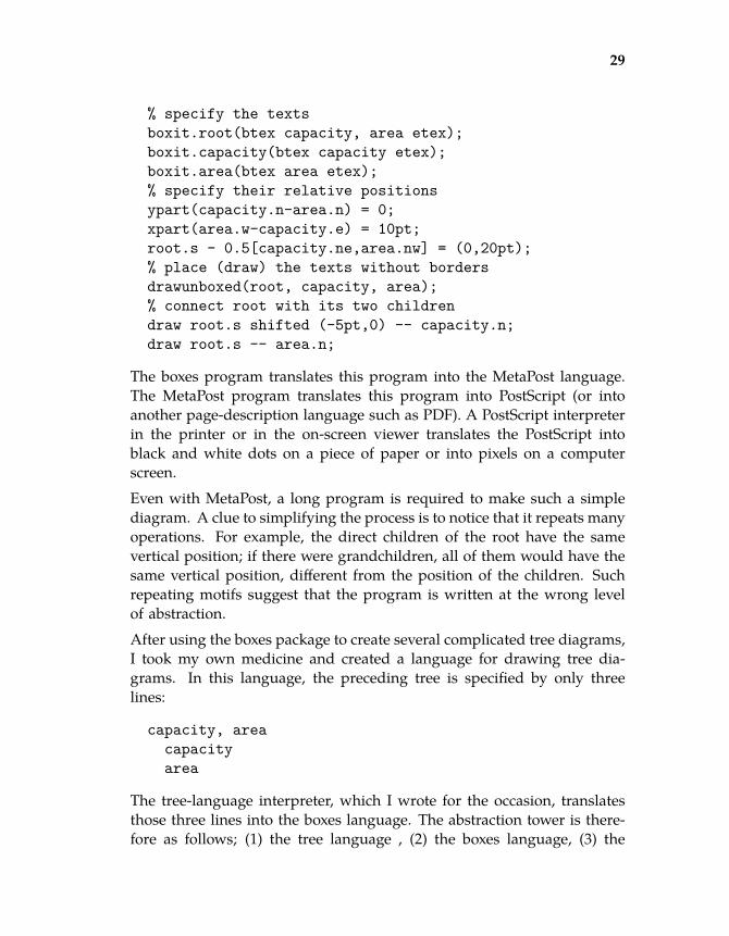
% specify the textsboxit.root(btex capacity, area etex);boxit.capacity(btex capacity etex);boxit.area(btex area etex);% specify their relative positionsypart(capacity.n-area.n) = 0;xpart(area.w-capacity.e) = 10pt;root.s - 0.5[capacity.ne,area.nw] = (0,20pt);% place (draw) the texts without bordersdrawunboxed(root, capacity, area);% connect root with its two childrendraw root.s shifted (-5pt,0) -- capacity.n;draw root.s -- area.n;

The boxes program translates this program into the MetaPost language.The MetaPost program translates this program into PostScript (or intoanother page-description language such as PDF). A PostScript interpreterin the printer or in the on-screen viewer translates the PostScript intoblack and white dots on a piece of paper or into pixels on a computerscreen.

Even with MetaPost, a long program is required to make such a simplediagram. A clue to simplifying the process is to notice that it repeats manyoperations. For example, the direct children of the root have the samevertical position; if there were grandchildren, all of them would have thesame vertical position, different from the position of the children. Suchrepeating motifs suggest that the program is written at the wrong levelof abstraction.

After using the boxes package to create several complicated tree diagrams,I took my own medicine and created a language for drawing tree dia-grams. In this language, the preceding tree is specified by only threelines:

capacity, areacapacityarea

The tree-language interpreter, which I wrote for the occasion, translatesthose three lines into the boxes language. The abstraction tower is there-fore as follows; (1) the tree language , (2) the boxes language, (3) the

38 38

38 38

30

2010-05-13 00:43:32 / rev b667c9e4c1f1+

MetaPost language, (4) the PostScript language, and (5) pixels on a screenor specks of toner on a page.

The tree minilanguage made constructing tree diagrams so easy that I cre-ated many diagrams to explain divide-and-conquer reasoning in Chap-ter 1 and to explain the subsequent ideas in this book. Here is a figurefrom Section 4.3.1:

jump height h

energy required

h m g

energy available

muscle mass

animal’s massm muscle fraction

energy densityin muscle

Its program in the tree minilanguage is short:

jump height $h$energy required$h$$m$$g$

energy availablemuscle massanimal’s mass $m$muscle fraction

energy density|in muscle

These 10 lines – simple to understand, write, and change – expand into34 lines of tedious, error-prone code in the boxes language. And theyexpand into 1732 lines of PostScript code! As Bertrand Russell said, “agood notation has a subtlety and suggestiveness which makes it almostseem like a live teacher” (quoted in [23, Chapter 8]).

39 39

39 39

31

2010-05-13 00:43:32 / rev b667c9e4c1f1+

2.1 Diagrams as abstractions

Diagrams are themselves a powerful kind of abstraction. Diagrams are anabstraction because they force one to discard irrelevant details, reducinga problem to what can be taken in at a glance. Diagrams are power-ful because our brain’s perceptual hardware is much more powerful thanits symbolic-processing hardware. There are evolutionary reasons for thisdifference. Our capacity for sequential analysis and therefore symbol pro-cessing took off with the advent of language – perhaps 105 years ago. Incontrast, visual processing has developed for millions of years among pri-mates alone (and even longer among vertebrates generally), and generalperceptual processing is even older.

Because of the extra development, visual learning can be rapid and long-lasting. For example, once you see the figure in Richard Gregory’s famousblack-and-white splotch picture [22], you will see it again very easily eventen years later. (I am being obscure about what the figure shows, in ordernot to spoil the surprise.) If only we could learn symbolic information asquickly. Although I now know the Navier–Stokes equation,

∂v∂t

+ (v·∇)v = −1ρ

∇p + ν∇2v,

learning it required many presentations!

Given the massive amount of mental hardware devoted to visual pro-cessing, a good problem-solving strategy is to translate problems intodiagrams and do a lot of the problem solving on the diagram – in otherwords, to make an abstraction and then to think using it. As an example,try the following problem.

You hike a path up a mountain over a 24-hour period, resting along the wayas you need. You sleep for 24 hours at the top. Then you walk down the samepath over the next 24 hours. Were you at any point on the path at the sametime of day on the way up and the way down? Alternatively, is it possibleto walk up and down on a careful schedule to ensure that there is no suchpoint?

It is hard to solve without making a diagram. To make the diagram,first decide on details that you do not care about – consider the situation“independently of its attributes.” For example, the day of the month, theyear, or the age of the hiker are irrelevant to the solution. All that mattersis the schedule on which you walk up and down, namely where are you

40 40

40 40

32

2010-05-13 00:43:32 / rev b667c9e4c1f1+

when? A particular walking and resting schedule can be abstracted toa function of t, the time of day, where the function gives your distancealong the path. Let u(t) be the schedule for hiking up the mountain, andd(t) be the schedule for hiking down the mountain. In this representation,the question is: Must u(t) = d(t) for some value of t? Or can you chooseu(t) and d(t) to avoid the equality for all values of t?

0 240

1

time (hours)

distance

With these abstractions, the question iscleaner, but it is not yet easy enough toanswer. A diagrammatic representationmakes the answer more obvious. Here isa diagram illustrating an upward sched-ule. Distance is measured from the bot-tom of the mountain (0) to the top ofthe mountain (1). According to the in-dicated schedule, you walked fast (theinitial slope), rested (the flat part), and then walked to the top.

0 240

1

time (hours)

distance

Here is a diagram illustrating a down-ward schedule. On this schedule, yourested (initial flat line), walked fast, thenwalked slowly to the bottom.

0 240

1

time (hours)

distance

And this diagram shows the upward anddownward schedules on the same dia-gram. Something interesting happens:The curves intersect! The intersectionpoint gives the time and location wherethe upward and downward schedules landedon the same point at the same time ofday (but on separate days).

Furthermore, the diagram shows that this pattern is general. No mat-ter what schedules you choose, the upward and downward paths mustcross. So the answer to the question is ‘Yes, there is always a point thatyou reached the same time on the upward and downward journeys’– an

41 41

41 41

33

2010-05-13 00:43:32 / rev b667c9e4c1f1+

answer hard to reach without abstracting away all the unessential detailsto make a diagram.

42 42

42 42

34

2010-05-13 00:43:32 / rev b667c9e4c1f1+

2.2 Recursion

Abstraction involves making reusable modules, ones that can be used forsolving other problems. The special case of abstraction where the otherproblem is a version of the original problem is known as recursion. Theterm is most common in computing, but recursion is broader than just acomputational method – as our first example illustrates.

2.2.1 Coin-flip game

The first example is the following game.Two people take turns flipping a (fair) coin. Whoever first turns over headswins. What is the probability that the first player wins?

As a first approach to finding the probability, get a feel for the game byplaying it. Here is one iteration of the game resulting from using a realcoin:

TH

The first player missed the chance to win by tossing tails; but the secondplayer won by tossing heads. Playing many such games may suggest apattern to what happens or suggest how to compute the probability.

However, playing many games by flipping a real coin becomes tedious. Acomputer can instead simulate the games using pseudorandom numbersas a substitute for a real coin. Here are several runs produced by acomputer program – namely, by a Python script coin-game.py. Eachline begins with 1 or 2 to indicate which player won the game; then theline gives the coin tosses that resulted in the win.

2 TH2 TH1 H2 TH1 TTH2 TTTH2 TH1 H1 H1 H

43 43

43 43

35

2010-05-13 00:43:32 / rev b667c9e4c1f1+

In these ten iterations, each player won five times. A reasonable conclu-sion, is that the game is fair: Each player has an equal chance to win.However, the conclusion cannot be believed too strongly based as it is ononly 10 games.

Let’s try 100 games. With only 10 games, one can quickly count thenumber of wins by each player by scanning the line beginnings. Butrather than repeating the process with 100 lines, here is a UNIX pipelineto do the work:

coin-game.py | head -100 | grep 1 | wc -l

Each run of this pipeline, because coin-game uses different pseudoran-dom numbers each time, produces a different total. The most recent invo-cation produced 68: In other words, player 1 won 68 times and player 2won 32 times. The probability of player 1’s winning now seems closer to2/3 than to 1/2.

start

H T

H T

H T

To find the exact value, first diagram the game as a tree.Each horizontal layer contains H and T, and representsone flip. The game ends at the leaves, when one playerhas tossed heads. The boldface H’s show the leaveswhere the first player wins, e.g. H, TTH, or TTTTH. Theprobabilities of each winning way are, respectively, 1/2,1/8, and 1/32. The infinite sum of these probabilities isthe probability p of the first player winning:

p =12

+18

+1

32+ · · · . (2.1)

This series can be summed using a familiar formula.

However, a more enjoyable analysis – which can explain the formula(Problem 2.1) – comes from noticing the presence of recursion: The treerepeats its structure one level down. That is, if the first player tosses tails,which happens with probability 1/2, then the second player starts thegame as if he or she were the first player. Therefore, the second playerwins the game with probability 1/2 times p (the factor of 1/2 is fromthe probability that the first player tosses tails). Because one of the twoplayers must win, the two winning probabilities p and p/2 add to unity.Therefore, p = 2/3, as conjectured from the simulation.

44 44

44 44

36

2010-05-13 00:43:32 / rev b667c9e4c1f1+

Problem 2.1 Summing a series using abstractionUse abstraction to find the sum of the infinite series

1 + r + r2 + r3 + · · · . (2.2)

2.2.2 Computational Recursion

The second example of recursion is an algorithm to multiply many-digitnumbers much more rapidly than is possible with the standard schoolmethod. The school method is sufficient for humans, for we rarely multi-ply large numbers by hand. However, computers are often called upon tomultiply gigantic numbers, whether in computing π to billions of digits orin public-key cryptography. I’ll introduce the new method by contrastingit with the school method on the example of 35 × 27.

In the school method, the product is written as

35 × 27 = (3 × 10 + 5) × (2 × 10 + 7). (2.3)

The product expands into four terms:

(3 × 10) × (2 × 10) + (3 × 10) × 7 + 5 × (2 × 10) + 5 × 7. (2.4)

Regrouping the terms by the powers of 10 gives

3 × 2 × 100 + (3 × 7 + 5 × 2) × 10 + 5 × 7. (2.5)

Then you remember the four one-digit multiplications 3 × 2, 3 × 7, 5 × 2,and 5 × 7, finding that

35 × 27 = 6 × 100 + 31 × 10 + 35 = 945. (2.6)

Unfortunately, the preceding description is cluttered with powers of 10obscuring the underlying pattern. Therefore, define a convenient notation(an abstraction!): Let y|x represent 10x+y and z|y|x represent 100z+10y+x.Then the school method runs as follows:

3|5 × 2|7 = 3 × 2∣∣∣ 3 × 7 + 5 × 2

∣∣∣ 5 × 7. (2.7)

This notation shows how school multiplication replaces a two-digit multi-plication with four one-digit multiplications. It would recursively replace

45 45

45 45

37

2010-05-13 00:43:32 / rev b667c9e4c1f1+

a four-digit multiplication with four two-digit multiplications. For exam-ple, using a modified | notation where y|x means 100y + x, the product3247 × 1798 becomes

32|47 × 17|98 = 32 × 17∣∣∣ 32 × 98 + 47 × 17

∣∣∣ 47 × 98. (2.8)

Each two-digit multiplication (of which there are four) would in turnbecome four one-digit multiplications. For example (and using the normaly|x = 10y + x notation),

3|2 × 1|7 = 3 × 2∣∣∣ 3 × 7 + 2 × 1

∣∣∣ 2 × 7. (2.9)

Thus, a four-digit multiplication becomes 16 one-digit multiplications.

Continuing the pattern, an eight-digit multiplication becomes four four-digit multiplications or, in the end, 64 one-digit multiplications. In gen-eral, an n-digit multiplication requires n2 one-digit multiplications. Thisrecursive algorithm seems so natural, perhaps because we learned it solong ago, that improvements are hard to imagine.

Surprisingly, a slight change in the method significantly improves it. Thekey is to retain the core idea of recursion but to improve the method ofdecomposition. Here is the improvement:

a1|a0 × b1|b0 = a1b1∣∣∣ (a1 + a0)(b1 + b0) − a1b1 − a0b0

∣∣∣ a0b0.

Before analyzing the improvement, let’s check that it is not nonsense byretrying the 35 × 27 example.

3|5 × 2|7 = 3 × 2∣∣∣ (3 + 5)(2 + 7) − 3 × 2 − 5 × 7

∣∣∣ 5 × 7.

Doing the five one-digit multiplications gives

3|5 × 2|7 = 6 | 31 | 35 = 6 × 100 + 31 × 10 + 35 = 945, (2.10)

just as it should.

At first glance, the method seems like a retrograde step because it re-quires five multiplications whereas the school method requires only four.However, the magic of the new method is that two multiplications areredundant: a1b1 and a0b0 are each computed twice. Therefore, the newmethod requires only three multiplications. The small change from fourto three multiplications, when used recursively, makes the new method

46 46

46 46

38

2010-05-13 00:43:32 / rev b667c9e4c1f1+

significantly faster: An n-digit multiplication requires roughly n1.58 one-digit multiplications (Problem 2.2). In contrast, the school algorithm re-quires n2 one-digit multiplications. The small decrease in the exponentfrom 2 to 1.58 has a large effect when n is large. For example, whenmultiplying billion-digit numbers, the ratio of n2 to nlog2 3 is roughly 5000.

Why would anyone multiply billion-digit numbers? One answer is tocompute π to a billion digits. Computing π to a huge number of digits,and comparing the result with the calculations of other supercomputers,is the standard way to verify the numerical hardware in a new supercom-puter.

The new algorithm is known as the Karatsuba algorithm after its inventor[13]. But even it is too slow for gigantic numbers. For large enough n,an algorithm using fast Fourier transforms is even faster than the Karat-suba algorithm. The so-called Schönhage–Strassen algorithm [27] requiresa time proportional to n log n log log n. High-quality libraries for large-number multiplication recursively use a combination of regular multipli-cation, Karatsuba, and Schönhage–Strassen, selecting the algorithm ac-cording to the number of digits.

Problem 2.2 Running time of the Karatsuba algorithmShow that the Karatsuba multiplication method requires nlog2 3

≈ n1.58 one-digitmultiplications.

47 47

47 47

39

2010-05-13 00:43:32 / rev b667c9e4c1f1+

2.3 Low-pass filters

The next example is an analysis that originated in the study of circuits(Section 2.3.1). After those ontological bonds are snipped – once thesubject is “considered independently of its original associations” – thecore idea (the abstraction) will be useful in understanding diverse naturalphenomena including temperature fluctuations (Section 2.3.2).

2.3.1 RC circuits

R

C

Vin VoutLinear circuits are composed of resistors, ca-pacitors, and inductors. Resistors are the onlytime-independent circuit element. To get time-dependent behavior – in other words, to get anyinteresting behavior – requires inductors or ca-pacitors. Here, as one of the simplest and mostwidely applicable circuits, we will analyze the behavior of an RC circuit.

The input signal is the voltage V0, a function of time t. The input signalpasses through the RC system and produces the output signal V1(t). Thedifferential equation that describes the relation between V0 and V1 is(from 8.02)

dV1

dt+

V1

RC=

V0

RC. (2.11)

This equation contains R and C only as the product RC. Therefore, itdoesn’t matter what R and C individually are; only their product RCmatters. Let’s make an abstraction and define a quantity τ as τ ≡ RC.

This time constant has a physical meaning. To see what it is, give thesystem the simplest nontrivial input: V0, the input voltage, has been zerosince forever; it suddenly becomes a constant V at t = 0; and it remainsat that value forever (t > 0). What is the output voltage V1? Until t = 0,the output is also zero. By inspection, you can check that the solution fort ≥ 0 is

V1 = V(1 − e−t/τ

). (2.12)

In other words, the output voltage exponentially approaches the inputvoltage. The rate of approach is determined by the time constant τ. Inparticular, after one time constant, the gap between the output and input

48 48

48 48

40

2010-05-13 00:43:32 / rev b667c9e4c1f1+

voltages shrinks by a factor of e. Alternatively, if the rate of approachremained its initial value, in one time constant the output would matchthe input (dotted line).

t

V

0

input

τ

The actual inputs provided by the world are more complex than a stepfunction. But many interesting real-world inputs are oscillatory (and itturns out that any input can be constructed by adding oscillatory inputs).So let’s analyze the effect of an oscillatory input V0(t) = Aeiωt, where A isa (possibly complex) constant called the amplitude, and ω is the angularfrequency of the oscillations. That complex-exponential notation reallymeans that the voltage is the real part of Aeiωt, but the ‘real part’ notationgets distracting if it is repeated in every equation, so traditionally it isomitted.

The RC system is linear – it is described by a linear differential equation– so the output will also oscillate with the same frequency ω. There-fore, write the output in the form Beiωt, where B is a (possibly complex)constant. Then substitute V0 and V1 into the differential equation

dV1

dt+

V1

RC=

V0

RC. (2.13)

After removing a common factor of eiωt, the result is

Biω +Bτ

=Aτ, (2.14)

or

B =A

1 + iωτ. (2.15)

This equation – a so-called transfer function – contains many generalizablepoints. First, ωτ is a dimensionless quantity. Second, when ωτ is smalland is therefore negligible compared to the 1 in the denominator, thenB ≈ A. In other words, the output almost exactly tracks the input.

Third, when ωτ is large, then the 1 in the denominator is negligible, so

49 49

49 49

41

2010-05-13 00:43:32 / rev b667c9e4c1f1+

B ≈ Aiωτ

. (2.16)

In this limit, the output variation (the amplitude B) is shrunk by a factor ofωτ in comparison to the input variation (the amplitude A). Furthermore,because of the i in the denominator, the output oscillations are delayedby 90 relative to the input oscillations (where 360 is a full period).Why 90 ? In the complex plane, dividing by i is equivalent to rotatingclockwise by 90 . As an example of this delay, if ωτ 1 and the inputvoltage oscillates with a period of 4hr, then the output voltage peaksroughly 1hr after the input peaks. Here is an example with ωτ = 4:

t

V input

In summary, this circuit allows low-frequency inputs to pass through tothe output almost unchanged, and it attenuates high-frequency inputs.It is called a low-pass filter: It passes low frequencies and blocks highfrequencies. The idea of a low-pass filter, now that we have abstracted itaway from its origin in circuit analysis, has many applications.

2.3.2 Temperature fluctuations

The abstraction of a low-pass filter resulting from the solutions to the RCdifferential equation are transferable. The RC circuit is, it turns out, amodel for heat flow; therefore, heat flow, which is everywhere, can beunderstood by using low-pass filters. As an example, I often prepare acup of tea but forget to drink it while it is hot. Slowly it cools toward roomtemperature and therefore becomes undrinkable. If I neglect the cup forstill longer – often it spends the night in the microwave, where I forgot it– it warms and cools with the room (for example, it will cool at night asthe house cools). A simple model of its heating and cooling is that heatflows in and out through the walls of the mug: the so-called thermalresistance. The heat is stored in the water and mug, which form a heatreservoir: the so-called thermal capacitance. Resistance and capacitanceare transferable abstractions.

50 50

50 50

42

2010-05-13 00:43:32 / rev b667c9e4c1f1+

If Rt is the thermal resistance and Ct is the thermal capacitance, theirproduct RtCt is, by analogy with the RC circuit, a thermal time constant τ.To measure it, heat up a mug of tea and watch how the temperature fallstoward room temperature. The time for the temperature gap to fall by afactor of e is the time constant τ. In my extensive experience of neglectingcups of tea, in 0.5hr an enjoyably hot cup of tea becomes lukewarm. Togive concrete temperatures to it, ‘enjoyably warm’ is perhaps 130 F, roomtemperature is 70 F, and lukewarm is perhaps 85 F. The temperature gapbetween the tea and the room started at 60 F and fell to 15 F – a factorof 4 decrease. It might have required 0.3hr to have fallen by a factor of e(roughly 2.72). This time is the time constant.How does the teacup respond to daily temperature variations? In thissystem, the input signal is the room’s temperature; it varies with a fre-quency of f = 1day−1. The output signal is the tea’s temperature. Thedimensionless parameter ωτ is, using ω = 2π f , given by

2π f︸︷︷︸ω

τ = 2π × 1day−1︸ ︷︷ ︸f

× 0.3hr︸︷︷︸τ

×1day24hr

, (2.17)

or approximately 0.1. In other words, the system is driven slowly (ω is notlarge enough to make ωτ near 1), so slowly that the inside temperaturealmost exactly follows the outside temperature.A situation showing the opposite extreme of behavior is the response ofa house to daily temperature variations. House walls are thicker thanteacup walls. Because thermal resistance, like electrical resistance, is pro-portional to length, the house walls give the house a large thermal re-sistance. However, the larger surface area of the house compared to theteacup more than compensates for the wall thickness, giving the house asmaller overall thermal resistance. Compared to the teacup, the house hasa much, much higher mass and much higher thermal capacitance. Theresulting time constant RtCt is much longer for the house than for theteacup. One study of houses in Greece quotes 86hr or roughly 4days asthe thermal time constant. That time constant must be for a well insulatedhouse.In Cape Town, South Africa, where the weather is mostly warm andhouses are often not heated even in the winter, the badly insulated housein which I lived had a thermal time constant of around 0.5day. Thedimensionless parameter ωτ is then

51 51

51 51

43

2010-05-13 00:43:32 / rev b667c9e4c1f1+

2π f︸︷︷︸ω

τ = 2π × 1day−1︸ ︷︷ ︸f

× 0.5day︸ ︷︷ ︸τ

, (2.18)

or approximately 3. In the (South African) winter, the outside temper-ature varied between 45 F and 75 F. This 30 F outside variation getsshrunk by a factor of 3, giving an inside variation of 10 F. This variationoccurred around the average outside temperature of 60 F, so the insidetemperature varied between 55 F and 65 F. Furthermore, if the coldestoutside temperature is at midnight, the coldest inside temperature is de-layed by almost 6hr (the one-quarter-period delay). Indeed, the housedid feel coldest early in the morning, just as I was getting up – as pre-dicted by this simple model of heat flow that is based on a circuit-analysisabstraction.

52 52

52 52

44

2010-05-13 00:43:32 / rev b667c9e4c1f1+

2.4 Summary and further problems

The diagram for the hiker has two names: a phase-space diagram or aspacetime diagram. Both types are useful in science and engineering.Spacetime diagrams, used in Einstein’s theory of relativity, are the sub-ject of the wonderful textbook [30]. They are the essential ingredient ina famous representation: Richard Feynman’s diagrams for calculationsin the theory of quantum electrodynamics (how radiation interacts withmatter). Those diagrams are discussed in [32]and [12].

The main ideas in this chapter:

For more on the value of diagrams, see [28]and [19].

Problem 2.3 Spacetime diagramsLearn about spacetime diagrams. My favorite source is Spacetime Physics [30].

Problem 2.4 Word processorsCompare WYSIWIG (what you see is what you get) word processors such asWordPerfect or Microsoft Word with document formatting systems such as TEXor ConTEXt (used to typeset this book).

Problem 2.5 Longest left-handed wordWhat is the longest word in the dictionary that can be typed with only the lefthand (on a qwerty keyboard)?

53 53

53 53

45

2010-05-13 00:43:32 / rev b667c9e4c1f1+

Part 2

Losslesscompression

3 Symmetry and conservation 47

4 Proportional reasoning 67

5 Dimensions 85

The first part discussed methods for organizing and therefore for manag-ing complexity. The remaining two parts discuss how to discard complexity.The discarded complexity can be actual complexity (Part 3) or it can beonly apparent complexity – whereupon discarding it does not discardinformation. Such lossless compression is the subject of this part.

54 54

54 54

46

2010-05-13 00:43:32 / rev b667c9e4c1f1+

The three methods are symmetry and conservation, proportional reason-ing, and dimensional analysis. Proportional reasoning and dimensionalanalysis are, additionally, examples of symmetry reasoning. Therefore,the next chapter introduces symmetry and conservation reasoning.

55 55

55 552010-05-13 00:43:32 / rev b667c9e4c1f1+

3Symmetry and conservation

3.1 Heat flow 483.2 Cube solitaire 503.3 Drag using conservation of energy 533.4 Cycling 563.5 Flight 59

Symmetry greatly simplifies any problem to which it applies – withoutany cost in accuracy. A classic example is the following story about theyoung Carl Friedrich Gauss. The story might be merely a legend, but it isso instructive that it ought to be true. One day when Gauss was 3 yearsold, the story goes, his schoolteacher wanted to occupy the students fora good while. He therefore asked them to compute the sum

S = 1 + 2 + 3 + · · · + 100,

and then sat back to enjoy a welcome break. To the teacher’s surprise,Gauss returned in a few minutes claiming that the sum is 5050. Was heright? If so, how did he compute the sum so quickly?Gauss noticed that the sum remains unchanged when the terms are addedbackward from highest to lowest. In other words,

S′ = 100 + 99 + 98 + · · · + 1

equals S. Then Gauss added the two sums:

S = 1 + 2 + 3 + · · · + 100+S = 100 + 99 + 98 + · · · + 1

2S = 101 + 101 + · · · + 101.

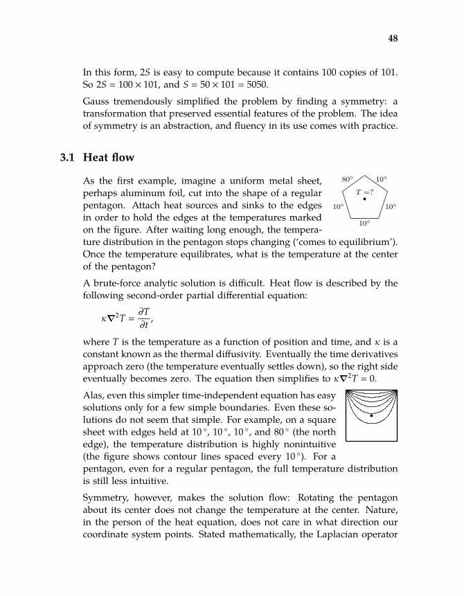
56 56

56 56

48

2010-05-13 00:43:32 / rev b667c9e4c1f1+

In this form, 2S is easy to compute because it contains 100 copies of 101.So 2S = 100 × 101, and S = 50 × 101 = 5050.

Gauss tremendously simplified the problem by finding a symmetry: atransformation that preserved essential features of the problem. The ideaof symmetry is an abstraction, and fluency in its use comes with practice.

3.1 Heat flow

80

10

10

10

10

T =?As the first example, imagine a uniform metal sheet,perhaps aluminum foil, cut into the shape of a regularpentagon. Attach heat sources and sinks to the edgesin order to hold the edges at the temperatures markedon the figure. After waiting long enough, the tempera-ture distribution in the pentagon stops changing (‘comes to equilibrium’).Once the temperature equilibrates, what is the temperature at the centerof the pentagon?

A brute-force analytic solution is difficult. Heat flow is described by thefollowing second-order partial differential equation:

κ∇2T =∂T∂t,

where T is the temperature as a function of position and time, and κ is aconstant known as the thermal diffusivity. Eventually the time derivativesapproach zero (the temperature eventually settles down), so the right sideeventually becomes zero. The equation then simplifies to κ∇2T = 0.

Alas, even this simpler time-independent equation has easysolutions only for a few simple boundaries. Even these so-lutions do not seem that simple. For example, on a squaresheet with edges held at 10 , 10 , 10 , and 80 (the northedge), the temperature distribution is highly nonintuitive(the figure shows contour lines spaced every 10 ). For apentagon, even for a regular pentagon, the full temperature distributionis still less intuitive.

Symmetry, however, makes the solution flow: Rotating the pentagonabout its center does not change the temperature at the center. Nature,in the person of the heat equation, does not care in what direction ourcoordinate system points. Stated mathematically, the Laplacian operator

57 57

57 57

49

2010-05-13 00:43:32 / rev b667c9e4c1f1+

∇2 is rotation invariant. Therefore, the following five orientations of thepentagon produce the identical temperature at the center:

80

10

1010

10 10

80

1010

10 10

10

8010

10 10

10

1080

10 10

10

1010

80

Now stack these sheets mentally, adding the temperatures that lie on topof each other to make the temperature profile of a new metal supersheet.On this new sheet, each edge has temperature

Tedge = 80 + 10 + 10 + 10 + 10 = 120 .

Solving for the resulting temperature distribution does not require solvingthe heat equation. All the edges are held at 120 , so the temperaturethroughout the sheet is 120 .

That result, with one more step, solves the original problem. The sym-metry operation is a rotation about the center of the pentagon, so thecenters overlap when the plates are stacked atop one another. Becausethe stacked plate has a temperature of 120 throughout, and the centersof the five stacked sheets align, each center is at T = 120/5 = 24.

Compare the symmetry solutions to Gauss’s sum and to this tempera-ture problem. The comparison will extract the transferable ideas (theuseful abstractions). First, both problems look complex upon first glance.Gauss’s sum has many terms, all different; the pentagon problem seemsto require solving a difficult partial differential equation. Second, bothproblems contain a symmetry operation. In Gauss’s sum, the symmetryoperation reversed the order of the terms; in the pentagon problem, thesymmetry operation rotated the pentagon by 72 . Third, the symmetryoperation leaves an important quantity unchanged: the sum S for Gauss’sproblem or the central temperature for the pentagon problem.

The moral of these two examples is as follows: When there is change, lookfor what does not change. That is, look for invariants. Then look for sym-metries: operations that leave these quantities unchanged.

58 58

58 58

50

2010-05-13 00:43:32 / rev b667c9e4c1f1+

3.2 Cube solitaire

1 0

00

0 0

00Here is a game of solitaire that illustrates the theme ofthis chapter. The following cube starts in the configu-ration in the margin; the goal is to make all vertices bemultiples of three simultaneously. The moves are all ofthe same form: Pick any edge and increment its twovertices by one. For example, if I pick the bottom edgeof the front face, then the bottom edge of the back face,the configuration becomes the first one in this series, then the second one:

2 1

00

0 0

00

2 1

00

1 1

00

Alas, neither configuration wins the game.

Can I win the cube game? If I can win, what is a sequence of moves endsin all vertices being multiples of 3? If I cannot win, how can that negativeresult be proved?

Brute force – trying lots of possibilities – looks overwhelming. Each moverequires choosing one of 12 edges, so there are 1210 sequences of tenmoves. Although that number is an overestimate, because the order ofthe moves does not affect the final state, even a somewhat lower numberwould still be overwhelming. I could push this line of reasoning byfiguring out how many possibilities there are, and how to list and checkthem if the number is not too large. But that approach is specific to thisproblem and unlikely to generalize to other problems.

1 0

00Instead of that specific approach, make the generic observa-tion that this problem is difficult because each move offersmany choices. The problem would be simpler with feweredges: for example, if the cube were a square. Can thissquare be turned into one where the four vertices are mul-tiples of 3? This problem is not the original problem, butsolving it might teach me enough to solve the cube. This hope moti-vates the following advice: When the going gets tough, the tough lower theirstandards.

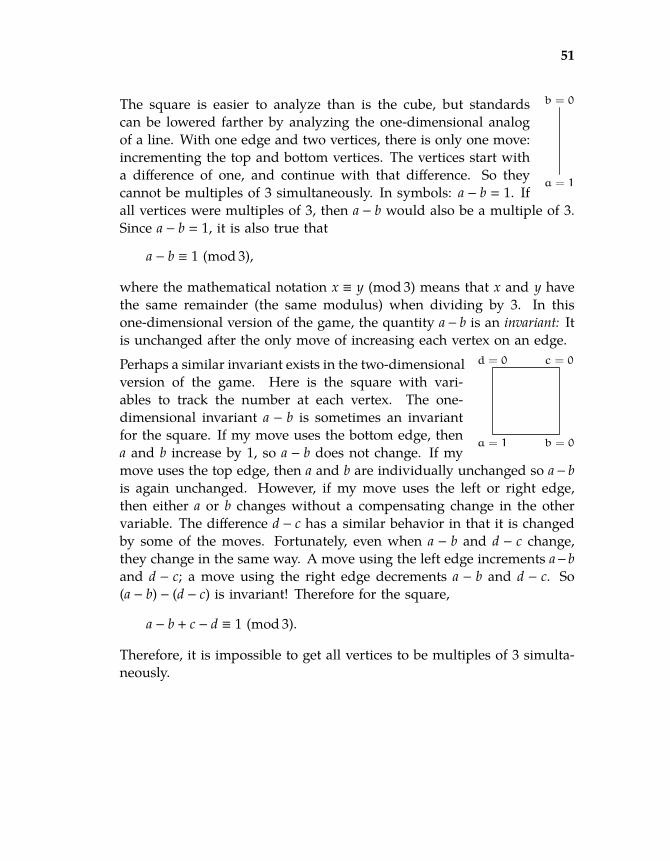
59 59

59 59

51

2010-05-13 00:43:32 / rev b667c9e4c1f1+

a = 1

b = 0The square is easier to analyze than is the cube, but standardscan be lowered farther by analyzing the one-dimensional analogof a line. With one edge and two vertices, there is only one move:incrementing the top and bottom vertices. The vertices start witha difference of one, and continue with that difference. So theycannot be multiples of 3 simultaneously. In symbols: a − b = 1. Ifall vertices were multiples of 3, then a − b would also be a multiple of 3.Since a − b = 1, it is also true that

a − b ≡ 1 (mod 3),

where the mathematical notation x ≡ y (mod 3) means that x and y havethe same remainder (the same modulus) when dividing by 3. In thisone-dimensional version of the game, the quantity a− b is an invariant: Itis unchanged after the only move of increasing each vertex on an edge.

a = 1 b = 0

c = 0d = 0Perhaps a similar invariant exists in the two-dimensionalversion of the game. Here is the square with vari-ables to track the number at each vertex. The one-dimensional invariant a − b is sometimes an invariantfor the square. If my move uses the bottom edge, thena and b increase by 1, so a − b does not change. If mymove uses the top edge, then a and b are individually unchanged so a− bis again unchanged. However, if my move uses the left or right edge,then either a or b changes without a compensating change in the othervariable. The difference d − c has a similar behavior in that it is changedby some of the moves. Fortunately, even when a − b and d − c change,they change in the same way. A move using the left edge increments a−band d − c; a move using the right edge decrements a − b and d − c. So(a − b) − (d − c) is invariant! Therefore for the square,

a − b + c − d ≡ 1 (mod 3).

Therefore, it is impossible to get all vertices to be multiples of 3 simulta-neously.

60 60

60 60

52

2010-05-13 00:43:32 / rev b667c9e4c1f1+

a = 1 b = 0

c = 0d = 0

e = 0 f = 0

g = 0h = 0The original three-dimensional solitaire game is alsounlikely to be winnable. The correct invariant showsthis impossibility. The quantity a−b+c−d+ f−g+h−egeneralizes the invariant for the square, and it ispreserved by all 12 moves. So

a − b + c − d + f − g + h − e ≡ 1 (mod 3)

forever. Therefore, all vertices cannot be made multiples of 3 simultane-ously.

Invariants – quantities that remain unchanged – are a powerful tool forsolving problems. Physics problems are also solitaire games, and invari-ants (conserved quantities) are essential in physics. Here is an example:In a frictionless world, design a roller-coaster track so that an unpoweredroller coaster, starting from rest, rises above its starting height. Perhaps aclever combination of loops and curves could make it happen.

The rules of the physics game are that the roller coaster’s position isdetermined by Newton’s second law of motion F = ma, where the forceson the roller coaster are its weight and the contact force from the track.In choosing the shape of the track, you affect the contact force on theroller coaster, and thereby its acceleration, velocity, and position. Thereare an infinity of possible tracks, and we do not want to analyze each oneto find the forces and acceleration.

An invariant – energy – vastly simplifies the analysis. No matter whattricks the track does, the kinetic plus potential energy

12

mv2 + mgh

is constant. The roller coaster starts with v = 0 and height hstart; it cannever rise above that height without violating the constancy of the energy.The invariant – the conserved quantity – solves the problem in one step,avoiding an endless analysis of an infinity of possible paths.

The moral of this section is the same as the moral of the previous section:When there is change, look for what does not change. That unchanging quantityis a new abstraction (Chapter 2). Finding invariants is a way to developpowerful abstractions.

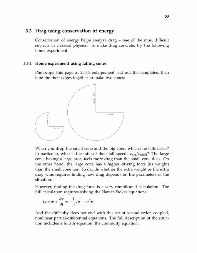
61 61

61 61

53

2010-05-13 00:43:32 / rev b667c9e4c1f1+

3.3 Drag using conservation of energy

Conservation of energy helps analyze drag – one of the most difficultsubjects in classical physics. To make drag concrete, try the followinghome experiment.

3.3.1 Home experiment using falling cones

Photocopy this page at 200% enlargement, cut out the templates, thentape the their edges together to make two cones:

r = 1 in

cuto

ut=

90 r = 2 in

cuto

ut=

90

When you drop the small cone and the big cone, which one falls faster?In particular, what is the ratio of their fall speeds vbig/vsmall? The largecone, having a large area, feels more drag than the small cone does. Onthe other hand, the large cone has a higher driving force (its weight)than the small cone has. To decide whether the extra weight or the extradrag wins requires finding how drag depends on the parameters of thesituation.

However, finding the drag force is a very complicated calculation. Thefull calculation requires solving the Navier–Stokes equations:

(v·O)v +∂v∂t

= −1ρOp + νO2v.

And the difficulty does not end with this set of second-order, coupled,nonlinear partial-differential equations. The full description of the situa-tion includes a fourth equation, the continuity equation:

62 62

62 62

54

2010-05-13 00:43:32 / rev b667c9e4c1f1+

O·v = 0.

One imposes boundary conditions, which include the motion of the ob-ject and the requirement that no fluid enters the object – and solves forthe pressure p and the velocity gradient at the surface of the object. Inte-grating the pressure force and the shear force gives the drag force.

In short, solving the equations analytically is difficult. I could spendhundreds of pages describing the mathematics to solve them. Even then,solutions are known only in a few circumstances, for example a sphereor a cylinder moving slowly in a viscous fluid or a sphere moving at anyspeed in an zero-viscosity fluid. But an inviscid fluid – what Feynmancalls ‘dry water’ [7, Chapter II-40] – is particularly irrelevant to real lifesince viscosity is the reason for drag, so an inviscid solution predictszero drag! Conservation of energy, supplemented with skillful lying, is asimple and quick alternative.

The analysis imagines an object of cross-sectional area A moving througha fluid at speed v for a distance d:

A volume ∼Ad

distance ∼ d

The drag force is the energy consumed per distance. The energy is con-sumed by imparting kinetic energy to the fluid, which viscosity eventu-ally removes from the fluid. The kinetic energy is mass times velocitysquared. The mass disturbed is ρAd, where ρ is the fluid density (here,the air density). The velocity imparted to the fluid is roughly the velocityof the disturbance, which is v. So the kinetic energy imparted to the fluidis ρAv2d, making the drag force

F ∼ ρAv2.

The analysis has a divide-and-conquer tree:

63 63

63 63

55

2010-05-13 00:43:32 / rev b667c9e4c1f1+

force ∼ E/d

ρAv2

energy imparted, ∼mv2

ρAv2d

mass disturbedρAd

densityρ

volumeAd

velocity imparted∼ v

distance d

The result that Fdrag ∼ ρv2A is enough to predict the result of the coneexperiment. The cones reach terminal velocity quickly (see Problem 7.10),so the relevant quantity in finding the fall time is the terminal velocity.From the drag-force formula, the terminal velocity is

v ∼

√Fdrag

ρA.

The cross-sectional areas are easy to measure with a ruler, and the ratiobetween the small- and large-cone terminal velocities is even easier. Theexperiment is set up to make the drag force easy to measure: Since thecones fall at their respective terminal velocities, the drag force equals theweight. So

v ∼

√WρA

.

Each cone’s weight is proportional to its cross-sectional area, because theyare geometrically similar and made out of the same piece of paper. Sothe terminal velocity v is independent of the area A: so the small andlarge cones should fall at the same speed.

To test this prediction, I stood on a table and dropped the two cones. Thefall lasted about two seconds, and they landed within 0.1 s of one another.So, the approximate conservation-of-energy analysis gains in plausibility(all the inaccuracies are hidden within the changing drag coefficient).

64 64

64 64

56

2010-05-13 00:43:32 / rev b667c9e4c1f1+

3.4 Cycling

This section discusses cycling as an example of how drag affects the per-formance of people as well as fleas. Those results will be used in theanalysis of swimming, the example of the next section.

What is the world-record cycling speed? Before looking it up, predict itusing armchair proportional reasoning. The first task is to define the kindof world record. Let’s say that the cycling is on a level ground using aregular bicycle, although faster speeds are possible using special bicyclesor going downhill.

To estimate the speed, make a model of where the energy goes. It goesinto rolling resistance, into friction in the chain and gears, and into drag.At low speeds, the rolling resistance and chain friction are probably im-portant. But the importance of drag rises rapidly with speed, so at high-enough speeds, drag is the dominant consumer of energy.

For simplicity, assume that drag is the only consumer of energy. Themaximum speed happens when the power supplied by the rider equalsthe power consumed by drag. The problem therefore divides into twoestimates: the power consumed by drag and the power that an athletecan supply.

The drag power Pdrag is related to the drag force:

Pdrag = Fdragv ∼ ρv3A.

It indeed rises rapidly with velocity, supporting the initial assumptionthat drag is the important effect at world-record speeds.

Setting Pdrag = Pathlete gives

vmax ∼

(Pathlete

ρA

)1/3

To estimate how much power an athlete can supply, I ran up one flightof stairs leading from the MIT Infinite Corridor. The Infinite Corridor,being an old building, has spacious high ceilings, so the vertical climb isperhaps h ∼ 4m (a typical house is 3m per storey). Leaping up the stairsas fast as I could, I needed t ∼ 5 s for the climb. My mass is 60kg, so mypower output was

65 65

65 65

57

2010-05-13 00:43:32 / rev b667c9e4c1f1+

Pauthor ∼potential energy supplied

time to deliver it

=mgh

t∼

60kg × 10ms−2× 4m

5 s∼ 500W.

Pathlete should be higher than this peak power since most authors are notOlympic athletes. Fortunately I’d like to predict the endurance record.An Olympic athlete’s long-term power might well be comparable to mypeak power. So I use Pathlete = 500W.

The remaining item is the cyclist’s cross-sectional area A. Divide the areainto width and height. The width is a body width, perhaps 0.4m. Aracing cyclist crouches, so the height is maybe 1m rather than a full 2m.So A ∼ 0.4m2.

Here is the tree that represents this analysis:vmax

Pathlete ∼ Estairs/tstairs

Estairs2400 J

m

60 kgg

10ms−2h

4m

tstairs5 s

Pdrag ∼ ρv3A

ρ

1 kgm−3

v A

0.4m2

Now combine the estimates to find the maximum speed. Putting in num-bers gives

vmax ∼

(Pathlete

ρA

)1/3

∼

(500W

1kgm−3 × 0.4m2

)1/3

.

The cube root might suggest using a calculator. However, massaging thenumbers simplifies the arithmetic enough to do it mentally. If only thepower were 400W or, instead, if the area were 0.5m! Therefore, in thewords of Captain Jean-Luc Picard, ‘make it so’. The cube root becomeseasy:

vmax ∼∼

(400W

1kgm−3 × 0.4m2

)1/3

∼ (1000m3 s−3)1/3 = 10ms−1.

66 66

66 66

58

2010-05-13 00:43:32 / rev b667c9e4c1f1+

So the world record should be, if this analysis has any correct physics init, around 10ms−1 or 22mph.

The world one-hour record – where the contestant cycles as far as pos-sible in one hour – is 49.7km or 30.9mi. The estimate based on drag isreasonable!

67 67

67 67

59

2010-05-13 00:43:32 / rev b667c9e4c1f1+

3.5 Flight

How far can birds and planes fly? The theory of flight is difficult andinvolves vortices, Bernoulli’s principle, streamlines, and much else. Thissection offers an alternative approach: use conservation estimate the en-ergy required to generate lift, then minimize the lift and drag contribu-tions to the energy to find the minimum-energy way to make a trip.

3.5.1 Lift

Instead of wading into the swamp of vortices, study what does not change.In this case, the vertical component of the plane’s momentum does notchange while it cruises at constant altitude.

Because of momentum conservation, a plane must deflect air downward.If it did not, gravity would pull the plane into the ground. By deflectingair downwards – which generates lift – the plane gets a compensating,upward recoil. Finding the necessary recoil leads to finding the energyrequired to produce it.

Imagine a journey of distance s. I calculate the energy to produce lift inthree steps:

1. How much air is deflected downward?

2. How fast must that mass be deflected downward in order to give theplane the needed recoil?

3. How much kinetic energy is imparted to that air?

The plane is moving forward at speed v, and it deflects air over an areaL2 where L is the wingspan. Why this area L2, rather than the cross-sectional area, is subtle. The reason is that the wings disturb the flowover a distance comparable to their span (the longest length). So whenthe plane travels a distance s, it deflects a mass of air

mair ∼ ρL2s.

The downward speed imparted to that mass must take away enough mo-mentum to compensate for the downward momentum imparted by grav-ity. Traveling a distance s takes time s/v, in which time gravity imparts adownward momentum Mgs/v to the plane. Therefore

68 68

68 68

60

2010-05-13 00:43:32 / rev b667c9e4c1f1+

mairvdown ∼Mgs

vso

vdown ∼Mgsvmair

∼MgsρvL2s

=MgρvL2 .

The distance s divides out, which is a good sign: The downward velocityof the air should not depend on an arbitrarily chosen distance!

The kinetic energy required to send that much air downwards is mairv2down.

That energy factors into (mairvdown)vdown, so

Elift ∼ mairvdown︸ ︷︷ ︸Mgs/v

vdown ∼Mgs

vMgρvL2︸︷︷︸vdown

=(Mg)2

ρv2L2 s.

Check the dimensions: The numerator is a squared force since Mg is aforce, and the denominator is a force, so the expression is a force timesthe distance s. So the result is an energy.

Interestingly, the energy to produce lift decreases with increasing speed.Here is a scaling argument to make that result plausible. Imagine dou-bling the speed of the plane. The fast plane makes the journey in one-halfthe time of the original plane. Gravity has only one-half the time to pullthe plane down, so the plane needs only one-half the recoil to stay aloft.Since the same mass of air is being deflected downward but with half thetotal recoil (momentum), the necessary downward velocity is a factor of 2lower for the fast plane than for the slow plane. This factor of 2 in speedlowers the energy by a factor of 4, in accordance with the v−2 in Elift.

3.5.2 Optimization including drag

The energy required to fly includes the energy to generate lift and tofight drag. I’ll add the lift and drag energies, and choose the speed thatminimizes the sum.

The energy to fight drag is the drag force times the distance. The dragforce is usually written as

Fdrag ∼ ρv2A,

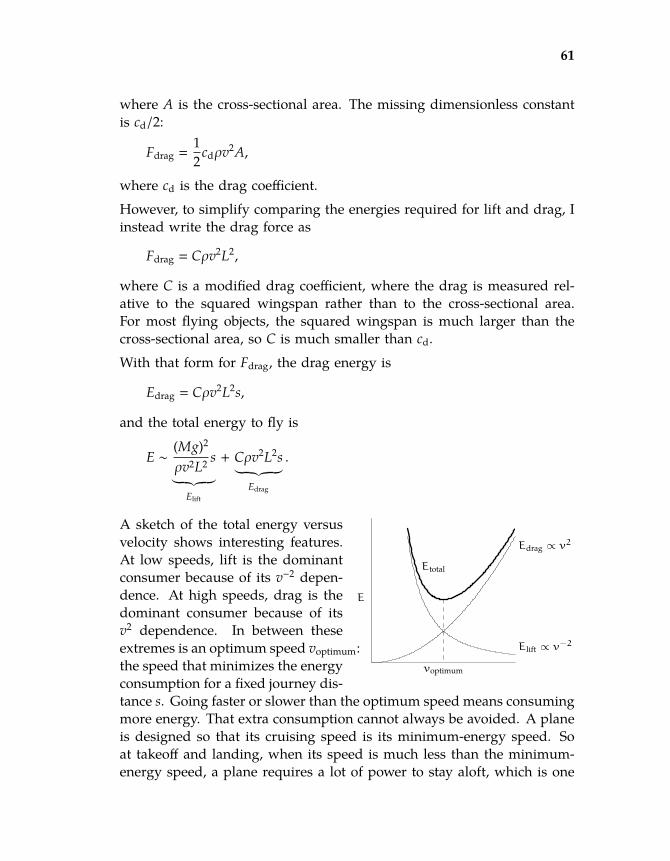
69 69

69 69

61

2010-05-13 00:43:32 / rev b667c9e4c1f1+

where A is the cross-sectional area. The missing dimensionless constantis cd/2:

Fdrag =12

cdρv2A,

where cd is the drag coefficient.

However, to simplify comparing the energies required for lift and drag, Iinstead write the drag force as

Fdrag = Cρv2L2,

where C is a modified drag coefficient, where the drag is measured rel-ative to the squared wingspan rather than to the cross-sectional area.For most flying objects, the squared wingspan is much larger than thecross-sectional area, so C is much smaller than cd.With that form for Fdrag, the drag energy is

Edrag = Cρv2L2s,

and the total energy to fly is

E ∼(Mg)2

ρv2L2 s︸ ︷︷ ︸Elift

+ Cρv2L2s︸ ︷︷ ︸Edrag

.

voptimum

Edrag ∝ v2

Elift ∝ v−2

Etotal

E

A sketch of the total energy versusvelocity shows interesting features.At low speeds, lift is the dominantconsumer because of its v−2 depen-dence. At high speeds, drag is thedominant consumer because of itsv2 dependence. In between theseextremes is an optimum speed voptimum:the speed that minimizes the energyconsumption for a fixed journey dis-tance s. Going faster or slower than the optimum speed means consumingmore energy. That extra consumption cannot always be avoided. A planeis designed so that its cruising speed is its minimum-energy speed. Soat takeoff and landing, when its speed is much less than the minimum-energy speed, a plane requires a lot of power to stay aloft, which is one

70 70

70 70

62

2010-05-13 00:43:32 / rev b667c9e4c1f1+

reason that the engines are so loud at takeoff and landing (another reasonis probably that the engine noise reflects off the ground and back to theplane).

The constraint, or assumption, that a plane travels at the minimum-energyspeed simplifies the expression for the total energy. At the minimum-energy speed, the drag and lift energies are equal. So

(Mg)2

ρv2L2 s ∼ Cρv2L2s,

or

Mg ∼ C1/2ρv2L2.

This constraint simplifies the total energy. Instead of simplifying the sum,simplify just the drag, which neglects only a factor of 2 since drag andlift are roughly equal at the minimum-energy speed. So

E ∼ Edrag ∼ Cρv2L2s ∼ C1/2Mgs.

This result depends in reasonable ways upon M, g, C, and s. First, liftovercomes gravity, and gravity produces the plane’s weight Mg. So Mgshould show up in the energy, and the energy should, and does, increasewhen Mg increases. Second, a streamlined plane should use less energythan a bluff, blocky plane, so the energy should, and does, increase asthe modified drag coefficient C increases. Third, since the flight is at aconstant speed, the energy should be, and is, proportional to the distancetraveled s.

3.5.3 Explicit computations

To get an explicit range, estimate the fuel fraction β, the energy densityE, and the drag coefficient C. For the fuel fraction I’ll guess β ∼ 0.4. ForE, look at the nutrition label on the back of a pack of butter. Butter isalmost all fat, and one serving of 11g provides 100Cal (those are ‘bigcalories’). So its energy density is 9kcal g−1. In metric units, it is 4 ·107 J kg−1. Including a typical engine efficiency of one-fourth gives

E ∼ 107 J kg−1.

71 71

71 71

63

2010-05-13 00:43:32 / rev b667c9e4c1f1+

The modified drag coefficient needs converting from easily available data.According to Boeing, a 747 has a drag coefficient of C′ ≈ 0.022, where thiscoefficient is measured using the wing area:

Fdrag =12

C′Awingρv2.

Alas, this formula is a third convention for drag coefficients, dependingon whether the drag is referenced to the cross-sectional area A, wing areaAwing, or squared wingspan L2.

It is easy to convert between the definitions. Just equate the standarddefinition

Fdrag =12

C′Awingρv2.

to our definition

Fdrag = CL2ρv2

to get

C =12

Awing

L2 C′ =12

lL

C′,

since Awing = Ll where l is the wing width. For a 747, l ∼ 10m andL ∼ 60m, so C ∼ 1/600.

Combine the values to find the range:

s ∼βE

C1/2g∼

0.4 × 107 J kg−1

(1/600)1/2 × 10ms−2 ∼ 107 m = 104 km.

The maximum range of a 747-400 is 13, 450km, so the approximate analy-sis of the range is unreasonably accurate.

72 72

72 72

64

2010-05-13 00:43:32 / rev b667c9e4c1f1+

Problem 3.1 IntegralsEvaluate these definite integrals:

a.∫ 10

−10x3e−x2

dx

b.∫∞

−∞

x3

1 + 7x2 + 18x8 dx

Problem 3.2 Number sumUse symmetry to find the sum of the integers between 200 and 300 (inclusive).

Problem 3.3 Heat equation

10

10

1010

80

T =?T =?

In lecture we used symmetry to argue that the tempera-ture at the center of the metal sheet is the average of thetemperatures of the sides.

Check this result by making a simulation or, if you arebold but crazy, by finding an analytic solution of the heatequation.

Problem 3.4 Symmetry for algebraUse symmetry to find (a − b)3.

Problem 3.5 Symmetry for second-order systemsThis problem analyzes the frequency of maximum gain for an LRC circuit or,equivalently, for a damped spring–mass system. The gain of such a system is theratio of the input amplitude to the output amplitude as a function of frequency.

If the output voltage is measured across the resistor, and you drive the circuitwith a voltage oscillating at frequency ω, the gain is (in a suitable system ofunits):

G(ω) =jω

1 + jω/Q − ω2 ,

where j =√−1 and Q is quality factor, a dimensionless measure of the damping.

Do not worry if you do not know where that gain formula comes from. Thepurpose of this problem is not its origin, but rather using symmetry to maximizeits magnitude.

a. Show that the magnitude of the gain is

|G(ω)| = ω√(1 − ω2

)2+ ω2/Q2

.

73 73

73 73

65

2010-05-13 00:43:32 / rev b667c9e4c1f1+

b. Find a variable substitution (a symmetry operation) ωnew = f (ω) that turns|G(ω)| into |H(ωnew)| such that G and H are the same function (i.e. they havethe same structure but with ω in G replaced by ωnew in H).

c. Use the form of that symmetry operation to maximize |G(ω)| without usingcalculus.

d. [Optional, for masochists!] Maximize |(Gω)| using calculus.

Problem 3.6 Inertia tensor[For those who know about inertia tensors.] Here is the inertia tensor (the generaliza-tion of moment of inertia) of a particular object, calculated in a lousy coordinatesystem: 4 0 0

0 5 40 4 5

a. Change coordinate systems to a set of principal axes. In other words, write

the inertia tensor as Ixx 0 00 Iyy 00 0 Izz

and give Ixx, Iyy, and Izz. Hint: What properties of a matrix are invariantwhen changing coordinate systems?

b. Give an example of an object with a similar inertia tensor. On Friday in classwe’ll have a demonstration.

Problem 3.7 Resistive grid

Ω

In an infinite grid of 1-ohm resistors, whatis the resistance measured across one re-sistor?

To measure resistance, an ohmmeter in-jects a current I at one terminal (for sim-plicity, say I = 1Å), removes the samecurrent from the other terminal, and mea-sures the resulting voltage difference V be-tween the terminals. The resistance is R =

V/I.

Hint: Use symmetry. But it’s still a hard problem!

74 74

74 742010-05-13 00:43:32 / rev b667c9e4c1f1+

75 75

75 752010-05-13 00:43:32 / rev b667c9e4c1f1+

4Proportional reasoning

4.1 Flight range versus size 684.2 Mountain heights 704.3 Jumping high 714.4 Drag 76

Symmetry wrings out excess, irrelevant complexity, and proportional rea-soning in one implementation of that philosophy. If an object moves withno forces on it (or if you walk steadily), then moving for twice as longmeans doubling the distance traveled. Having two changing quantitiescontributes complexity. However, the ratio distance/time, also known asthe speed, is independent of the time. It is therefore simpler than distanceor time. This conclusion is perhaps the simplest example of proportionalreasoning, where the proportional statement is

distance ∝ time.

Using symmetry has mitigated complexity. Here the symmetry operationis ‘change for how long the object move (or how long you walk)’. This op-eration should not change conclusions of an analysis. So, do the analysisusing quantities that themselves are unchanged by this symmetry opera-tion. One such quantity is the speed, which is why speed is such a usefulquantity.Similarly, in random walks and diffusion problems, the mean-square dis-tance traveled is proportional to the time travelled:

〈x2〉 ∝ t.

So the interesting quantity is one that does not change when t changes:

76 76

76 76

68

2010-05-13 00:43:32 / rev b667c9e4c1f1+

interesting quantity ≡ 〈x2〉

t.

This quantity is so important that it is given a name – the diffusion con-stant – and is tabulated in handbooks of material properties.

4.1 Flight range versus size

How does the range depend on the size of the plane? Assume that allplanes are geometrically similar (have the same shape) and therefore differonly in size.

Since the energy required to fly a distance s is E ∼ C1/2Mgs, a tank of fuelgives a range of

s ∼ Etank

C1/2Mg.

Let β be the fuel fraction: the fraction of the plane’s mass taken up byfuel. Then Mβ is the fuel mass, and MβE is the energy contained in thefuel, where E is the energy density (energy per mass) of the fuel. Withthat notation, Etank ∼MβE and

s ∼MβE

C1/2Mg=

βE

C1/2g.

Since all planes, at least in this analysis, have the same shape, their mod-ified drag coefficient C is also the same. And all planes face the samegravitational field strength g. So the denominator is the same for allplanes. The numerator contains β and E. Both parameters are the samefor all planes. So the numerator is the same for all planes. Therefore

s ∝ 1.

All planes can fly the same distance!

Even more surprising is to apply this reasoning to migrating birds. Hereis the ratio of ranges:

splanesbird

∼βplaneβbird

Eplane

Ebird

(Cplane

Cbird

)−1/2

.

Take the factors in turn. First, the fuel fraction βplane is perhaps 0.3 or0.4. The fuel fraction βbird is probably similar: A well-fed bird having

77 77

77 77

69

2010-05-13 00:43:32 / rev b667c9e4c1f1+

fed all summer is perhaps 30 or 40% fat. So βplane/βbird ∼ 1. Second,jet fuel energy density is similar to fat’s energy density, and plane en-gines and animal metabolism are comparably efficient (about 25%). SoEplane/Ebird ∼ 1. Finally, a bird has a similar shape to a plane – it is not agreat approximation, but it has the virtue of simplicity. So Cbird/Cplane ∼ 1.

Therefore, planes and well-fed, migrating birds should have the samemaximum range! Let’s check. The longest known nonstop flight byan animal is 11, 570km, made by a bar-tailed godwit from Alaska toNew Zealand (tracked by satellite). The maximum range for a 747-400is 13, 450km, only slightly longer than the godwit’s range.

78 78

78 78

70

2010-05-13 00:43:32 / rev b667c9e4c1f1+

4.2 Mountain heights

The next example of proportional reasoning explains why mountains can-not become too high. Assume that all mountains are cubical and made ofthe same material. Making that assumption discards actual complexity,the topic of ??. However, it is a useful approximation.

To see what happens if a mountain gets too large, estimate the pressureat the base of the mountain. Pressure is force divided by area, so estimatethe force and the area.

The area is the easier estimate. With the approximation that all moun-tains are cubical and made of the same kind of rock, the only parameterdistinguishing one mountain from another is its side length l. The areaof the base is then l2.

Next estimate the force. It is proportional to the mass:

F ∝ m.

In other words, F/m is independent of mass, and that independence iswhy the proportionality F ∝ m is useful. The mass is proportional to l3:

m ∝ volume ∼ l3.

In other words, m/l3 is independent of l; this independence is why theproportionality m ∝ l3 is useful. Therefore

F ∝ l3.

79 79

79 79

71

2010-05-13 00:43:32 / rev b667c9e4c1f1+

pressure∝ l

force∝ l3

mass∝ l3

volume∝ l3

area∝ l2

The force and area results show that the pressure is pro-portional to l:

p ∼ FA∝

l3

l2= l.

With a large-enough mountain, the pressure is larger thanthe maximum pressure that the rock can withstand. Thenthe rock flows like a liquid, and the mountain cannot growtaller.

This estimate shows only that there is a maximum heightbut it does not compute the maximum height. To do thatnext step requires estimating the strength of rock. Laterin this book when we estimate the strength of materials, Irevisit this example.

This estimate might look dubious also because of the assumption thatmountains are cubical. Who has seen a cubical mountain? Try a reason-able alternative, that mountains are pyramidal with a square base of sidel and a height l, having a 45 slope. Then the volume is l3/3 instead of l3but the factor of one-third does not affect the proportionality between force andlength. Because of the factor of one-third, the maximum height will behigher for a pyramidal mountain than for a cubical mountain. However,there is again a maximum size (and height) of a mountain. In general,the argument for a maximum height requires only that all mountains aresimilar – are scaled versions of each other – and does not depend on theshape of the mountain.

4.3 Jumping high

We next use proportional reasoning to understand how high animalsjump, as a function of their size. Do kangaroos jump higher than fleas?We study a jump from standing (or from rest, for animals that do notstand); a running jump depends on different physics. This problem looksunderspecified. The height depends on how much muscle an animal has,how efficient the muscles are, what the animal’s shape is, and much else.The first subsection introduces a simple model of jumping, and the sec-ond refines the model to consider physical effects neglected in the crudeapproximations.

80 80

80 80

72

2010-05-13 00:43:32 / rev b667c9e4c1f1+

4.3.1 Simple model

We want to determine only how jump height varies with body mass. Eventhis problem looks difficult; the height still depends on muscle efficiency,and so on. Let’s see how far we get by just plowing along, and usingsymbols for the unknown quantities. Maybe all the unknowns cancel.

We want an equation for the height h in the form h ∼ mβ, where m is theanimal’s mass and β is the so-called scaling exponent.

m

m

h

Jumping requires energy, which must be provided by muscles.This first, simplest model equates the required energy to theenergy supplied by the animal’s muscles.

The required energy is the easier estimation: An animal of massm jumping to a height h requires an energy Ejump ∝ mh. Becauseall animals feel the same gravity, this relation does not containthe gravitational acceleration g. You could include it in theequation, but it would just carry through the equations likeunused baggage on a trip.

The available energy is the harder estimation. To find it, divide andconquer. It is the product of the muscle mass and of the energy per mass(the energy density) stored in muscle.

To approximate the muscle mass, assume that a fixed fraction of an ani-mals mass is muscle, i.e. that this fraction is the same for all animals. Ifα is the fraction, then

mmuscle ∼ αm

or, as a proportionality,

mmuscle ∝ m,

where the last step uses the assumption that all animals have the same α.

For the energy per mass, assume again that all muscle tissues are thesame: that they store the same energy per mass. If this energy per massis E, then the available energy is

Eavail ∼ Emmuscle

or, as a proportionality,

81 81

81 81

73

2010-05-13 00:43:32 / rev b667c9e4c1f1+

Eavail ∝ mmuscle,

where this last step uses the assumption that all muscle has the sameenergy density E.

Here is a tree that summarizes this model:jump height h

energy required

h m g

energy available

muscle mass

animal’s massm muscle fraction

energy densityin muscle

Now finish propagating toward the root. The available energy is

Eavail ∝ m.

So an animal with three times the mass of another animal can storeroughly three times the energy in its muscles, according to this simplemodel.

Now compare the available and required energies to find how the jumpheight as a function of mass. The available energy is

Eavail ∝ m

and the required energy is

Erequired ∝ mh.

Equate these energies, which is an application of conservation of energy.Then mh ∝ m or

h ∝ m0.

In other words, all animals jump to the same height.

82 82

82 82

74

2010-05-13 00:43:32 / rev b667c9e4c1f1+

flea

click beetle

locust human

101

102

h(c

m)

10−4 10−1 102m (g)

The result, that all animals jump to thesame height, seems surprising. Our intu-ition tells us that people should be ableto jump higher than locusts. The graphshows jump heights for animals of var-ious sizes and shapes [source: Scaling:Why Animal Size is So Important [26, p. 178].Here is the data:Animal Mass (g) Height (cm)Flea 5 ·10−4 20Click beetle 4 ·10−2 30Locust 3 59Human 7 ·104 60

The height varies almost not at all when compared to variation in mass,so our result is roughly correct! The mass varies more than eight ordersof magnitude (a factor of 108), yet the jump height varies only by a factorof 3. The predicted scaling of constant h (h ∝ 1) is surprisingly accurate.

83 83

83 83

75

2010-05-13 00:43:32 / rev b667c9e4c1f1+

4.3.2 Power limits

Power production might also limit the jump height. In the precedinganalysis, energy is the limiting reagent: The jump height is determinedby the energy that an animal can store in its muscles. However, even if theanimal can store enough energy to reach that height, the muscles mightnot be able to deliver the energy rapidly enough. This section presents asimple model for the limit due to limited power generation.

Once again we’d like to find out how power P scales (varies) with the sizel Power is energy per time, so the power required to jump to a height his

P ∼energy required to jump to height h

time over which the energy is delivered.

The energy required is E ∼ mgh. The mass is m ∝ l3. The gravitationalacceleration is independent of l. And, in the energy-limited model, theheight h is independent of l. Therefore E ∝ l3.

The delivery time is how long the animal is in contact with the ground,because only during contact can the ground exert a force on the animal.So, the animal crouches, extends upward, and finally leaves the ground.The contact time is the time during which the animal extends upward.Time is length over speed, so

tdelivery ∼extension distanceextension speed

.

The extension distance is roughly the animal’s size l. The extension speedis roughly the takeoff velocity. In the energy-limited model, the takeoffvelocity is the same for all animals:

vtakeoff ∝ h1/2∝ l0.

So

tdelivery ∝ l.

The power required is P ∝ l3/l = l2.

That proportionality is for the power itself, but a more interesting scalingis for the specific power: the power per mass. It is

84 84

84 84

76

2010-05-13 00:43:32 / rev b667c9e4c1f1+

Pm∝

l2

l3= l−1.

Ah, smaller animals need a higher specific power!

A model for power limits is that all muscle can generate the same maxi-mum power density (has the same maximum specific power). So a small-enough animal cannot jump to its energy-limited height. The animal canstore enough energy in its muscles, but cannot release it quickly enough.

More precisely, it cannot do so unless it finds an alternative method forreleasing the energy. The click beetle, which is toward the small end inthe preceding graph and data set, uses the following solution. It storesenergy in its shell by bending the shell, and maintains the bending like aratchet would (holding a structure motionless does require energy). Thisstorage can happen slowly enough to avoid the specific-power limit, butwhen the beetle releases the shell and the shell snaps back to its restingposition, the energy is released quickly enough for the beetle to rise to itsenergy-limited height.

But that height is less than the height for locusts and humans. Indeed, thelargest deviations from the constant-height result happen at the low-massend, for fleas and click beetles. To explain that discrepancy, the modelneeds to take into account another physical effect: drag.

4.4 Drag

4.4.1 Jumping fleas

The drag force

F ∼ ρAv2

affects the jumps of small animals more than it affects the jumps of peo-ple. A comparison of the energy required for the jump with the energyconsumed by drag explains why.

The energy that the animal requires to jump to a height h is mgh, if we usethe gravitational potential energy at the top of the jump; or it is ∼ mv2, ifwe use the kinetic energy at takeoff. The energy consumed by drag is

85 85

85 85

77

2010-05-13 00:43:32 / rev b667c9e4c1f1+

Edrag ∼ ρv2A︸︷︷︸Fdrag

×h.

The ratio of these energies measures the importance of drag. The ratio is

Edrag

Erequired∼ρv2Ahmv2 =

ρAhm

.

Since A is the cross-sectional area of the animal, Ah is the volume of airthat it sweeps out in the jump, and ρAh is the mass of air swept out inthe jump. So the relative importance of drag has a physical interpretationas a ratio of the mass of air displaced to the mass of the animal.

To find how this ratio depends on animal size, rewrite it in terms of theanimal’s side length l. In terms of side length, A ∼ l2 and m ∝ l3. Whatabout the jump height h? The simplest analysis predicts that all animalshave the same jump height, so h ∝ l0. Therefore the numerator ρAh is∝ l1, the denominator m is ∝ l3, and

Edrag

Erequired∝

l2

l3= l−1.

So, small animals have a large ratio, meaning that drag affects the jumpsof small animals more than it affects the jumps of large animals. Themissing constant of proportionality means that we cannot say at what sizean animal becomes ‘small’ for the purposes of drag. So the calculation sofar cannot tell us whether fleas are included among the small animals.

The jump data, however, substitutes for the missing constant of propor-tionality. The ratio is

Edrag

Erequired∼ρAhm∼

ρl2hρanimall3

.

It simplifies toEdrag

Erequired∼

ρ

ρanimal

hl.

As a quick check, verify that the dimensions match. The left side is a ratioof energies, so it is dimensionless. The right side is the product of twodimensionless ratios, so it is also dimensionless. The dimensions match.

86 86

86 86

78

2010-05-13 00:43:32 / rev b667c9e4c1f1+

Now put in numbers. A density of air is ρ ∼ 1kgm−3. The density ofan animal is roughly the density of water, so ρanimal ∼ 103 kgm−3. Thetypical jump height – which is where the data substitutes for the constantof proportionality – is 60 cm or roughly 1m. A flea’s length is about 1mmor l ∼ 10−3 m. So

Edrag

Erequired∼

1kgm−3

103 kgm−31m

10−3 m∼ 1.

The ratio being unity means that if a flea would jump to 60 cm, overcom-ing drag would require roughly as much as energy as would the jumpitself in vacuum.

Drag provides a plausible explanation for why fleas do not jump as highas the typical height to which larger animals jump.

87 87

87 87

79

2010-05-13 00:43:32 / rev b667c9e4c1f1+

4.4.2 Swimming

A previous section’s analysis of cycling helps predict the world-recordspeed for swimming.

vmax ∼

(Pathlete

ρA

)1/3

.

To evaluate the maximum speed for swimming, one could put in a newρ and A directly into that formula. However, that method replicates thework of multiplying, dividing, and cube-rooting the various values.

Instead it is instructive to scale the numerical result for cycling by look-ing at how the maximum speed depends on the parameters of the sit-uation. In other words, I’ll use the formula for vmax to work out theratio vswimmer/vcyclist, and then use that ratio along with vcyclist to work outvswimmer.

The speed vmax is

vmax ∼

(Pathlete

ρA

)1/3

.

So the ratio of swimming and cycling speeds is

vswimmer

vcyclist∼

(Pswimmer

Pcyclist

)1/3

×

(ρswimmer

ρcyclist

)−1/3

×

(Aswimmer

Acyclist

)−1/3

.

Estimate each factor in turn. The first factor accounts for the relative ath-letic prowess of swimmers and cyclists. Let’s assume that they generateequal amounts of power; then the first factor is unity. The second factoraccounts for the differing density of the mediums in which each athletemoves. Roughly, water is 1000 times denser than air. So the second factorcontributes a factor of 0.1 to the speed ratio. If the only factors were thefirst two, then the swimming world record would be about 1ms−1.

Let’s compare with reality. The actual world record for a 1500-m freestyle(in a 50-m pool) is 14m34.56s set in July 2001 by Grant Hackett. Thatspeed is 1.713ms−1, significantly higher than the prediction of 1ms−1.

The third factor comes to the rescue by accounting for the relative profileof a cyclist and a swimmer. A swimmer and a cyclist probably have thesame width, but the swimmer’s height (depth in the water) is perhaps

88 88

88 88

80

2010-05-13 00:43:32 / rev b667c9e4c1f1+

one-sixth that of a crouched cyclist. So the third factor contributes 61/3 tothe predicted speed, making it 1.8ms−1.

This prediction is close to the actual record, closer to reality than onemight expect given the approximations in the physics, the values, and thearithmetic. However, the accuracy is a result of the form of the estimate,that the maximum speed is proportional to the cube root of the athlete’spower and the inverse cube root of the cross-sectional area. Errors ineither the power or area get compressed by the cube root. For example,the estimate of 500W might easily be in error by a factor of 2 in eitherdirection. The resulting error in the maximum speed is 21/3 or 1.25, anerror of only 25%. The cross-sectional area of a swimmer might be inerror by a factor of 2 as well, and this mistake would contribute onlya 25% error to the maximum speed. [With luck, the two errors wouldcancel!]

4.4.3 Flying

In the next example, I scale the drag formula to estimate the fuel efficiencyof a jumbo jet. Rather than estimating the actual fuel consumption, whichwould produce a large, meaningless number, it is more instructive toestimate the relative fuel efficiency of a plane and a car.

Assume that jet fuel goes mostly to fighting drag. This assumption is notquite right, so at the end I’ll discuss it and other troubles in the analysis.The next step is to assume that the drag force for a plane is given by thesame formula as for a car:

Fdrag ∼ ρv2A.

Then the ratio of energy consumed in travelling a distance d isEplane

Ecar∼ρup−highρlow

×

(vplanevcar

)2×

Aplane

Acar×

dd.

Estimate each factor in turn. The first factor accounts for the lower airdensity at a plane’s cruising altitude. At 10km, the density is roughly one-third of the sea-level density, so the first factor contributes 1/3. The secondfactor accounts for the faster speed of a plane. Perhaps vplane ∼ 600mphand vcar ∼ 60mph, so the second factor contributes a factor of 100. Thethird factor accounts for the greater cross-sectional area of the plane. Asa reasonable estimate

89 89

89 89

81

2010-05-13 00:43:32 / rev b667c9e4c1f1+

Aplane ∼ 6m × 6m = 36m2,

whereas

Acar ∼ 2m × 1.5m = 3m2,

so the third factor contributes a factor of 12. The fourth factor contributesunity, since we are analyzing the plane and car making the same trip(New York to Los Angeles, say).

The result of the four factors isEplane

Ecar∼

13× 100 × 12 ∼ 400.

A plane looks incredibly inefficient. But I neglected the number of people.A jumbo jet takes carries 400 people; a typical car, at least in California,carries one person. So the plane and car come out equal!

This analysis leaves out many effects. First, jet fuel is used to generate liftas well as to fight drag. However, as a later analysis will show, the energyconsumed in generating lift is comparable to the energy consumed infighting drag. Second, a plane is more streamlined than a car. Thereforethe missing constant in the drag force Fdrag ∼ ρv2A is smaller for a planethan for a car. our crude analysis of drag has not included this effect.Fortunately this error compensates, or perhaps overcompensates, for theerror in neglecting lift.

90 90

90 90

82

2010-05-13 00:43:32 / rev b667c9e4c1f1+

More on proportional reasoning

Problem 4.1 Raindrop speed

a. How does a raindrop’s terminal velocity v depend on the raindrop’s radiusr?

b. Estimate the terminal speed for a typical raindrop.

c. How could you check your estimate in part (b)?

Problem 4.2 MountainsLook up the height of the tallest mountain on earth, Mars, and Venus, andexplain any pattern in the three values.

Problem 4.3 Highway vs city drivingIn lecture we derived a measure of how important drag is for a car moving atspeed v for a distance d:

Edrag

Ekinetic∼ρv2Admcarv2 .

a. Show that the ratio is equivalent to the ratio

mass of the air displacedmass of the car

and to the ratioρairρcar×

dlcar

,

where ρcar is the density of the car (i.e. its mass divided by its volume) andlcar is the length of the car.

b. Make estimates for a typical car and find the distance d at which the ratiobecomes significant (say, roughly 1). How does the distance compare with thedistance between exits on the highway and between stop signs or stoplightson city streets?

Problem 4.4 Gravity on the moonIn this problem you use a scaling argument to estimate the strength of gravityon the surface of the moon.

a. Assume that a planet is a uniform sphere. What is the proportionalitybetween the gravitational acceleration g at the surface of a planet and theplanet’s radius R and density ρ?

b. Write the ratio gmoon/gearth as a product of dimensionless factors as in theanalysis of the fuel efficiency of planes.

91 91

91 91

83

2010-05-13 00:43:32 / rev b667c9e4c1f1+

c. Estimate those factors and estimate the ratio gmoon/gearth, then estimategmoon. [Hint: To estimate the radius of the moon, whose angular size youcan estimate by looking at it, you might find it useful to know that the moonis 4 ·108 m distant from the earth.]

d. Look up gmoon and compare the value to your estimate, venturing an expla-nation for any discrepancy.

Problem 4.5 Checking plane fuel-efficiency calculationThis problem offers two more methods to estimate the fuel efficiency of a plane.

a. Use the cost of a plane ticket to estimate the fuel efficiency of a 747, inpassenger–miles per gallon.

b. According to Wikipedia, a 747-400 can hold up to 2·105` of fuel for a maximumrange of 1.3 · 104 km. Use that information to estimate the fuel efficiency ofthe 747, in passenger–miles per gallon.

How do these values compare with the rough result from lecture, that the fuelefficiency is comparable to the fuel efficiency of a car?

92 92

92 922010-05-13 00:43:32 / rev b667c9e4c1f1+

93 93

93 932010-05-13 00:43:32 / rev b667c9e4c1f1+

5Dimensions

5.1 Power of multinational corporations 855.2 Dimensionless groups 875.3 Hydrogen atom 925.4 Bending of light by gravity 975.5 Buckingham Pi theorem 1045.6 Drag 105

5.1 Power of multinational corporations

Critics of globalization often make the following comparison [17] to provethe excessive power of multinational corporations:

In Nigeria, a relatively economically strong country, the GDP [gross domesticproduct] is $99 billion. The net worth of Exxon is $119 billion. “When multi-nationals have a net worth higher than the GDP of the country in which theyoperate, what kind of power relationship are we talking about?” asks LauraMorosini.

Before continuing, explore the following question:

What is the most egregious fault in the comparison between Exxon and Nigeria?

The field is competitive, but one fault stands out. It becomes evident afterunpacking the meaning of GDP. A GDP of $99 billion is shorthand fora monetary flow of $99 billion per year. A year, which is the time forthe earth to travel around the sun, is an astronomical phenomenon thathas been arbitrarily chosen for measuring a social phenomenon—namely,monetary flow.

94 94

94 94

86

2010-05-13 00:43:32 / rev b667c9e4c1f1+

Suppose instead that economists had chosen the decade as the unit oftime for measuring GDP. Then Nigeria’s GDP (assuming the flow remainssteady from year to year) would be roughly $1 trillion per decade andbe reported as $1 trillion. Now Nigeria towers over Exxon, whose punyassets are a mere one-tenth of Nigeria’s GDP. To deduce the oppositeconclusion, suppose the week were the unit of time for measuring GDP.Nigeria’s GDP becomes $2 billion per week, reported as $2 billion. Nowpuny Nigeria stands helpless before the mighty Exxon, 50-fold larger thanNigeria.A valid economic argument cannot reach a conclusion that depends onthe astronomical phenomenon chosen to measure time. The mistake liesin comparing incomparable quantities. Net worth is an amount: It hasdimensions of money and is typically measured in units of dollars. GDP,however, is a flow or rate: It has dimensions of money per time andtypical units of dollars per year. (A dimension is general and independentof the system of measurement, whereas the unit is how that dimension ismeasured in a particular system.) Comparing net worth to GDP comparesa monetary amount to a monetary flow. Because their dimensions differ,the comparison is a category mistake [] and is therefore guaranteed togenerate nonsense.

Problem 5.1 Units or dimensions?Are meters, kilograms, and seconds units or dimensions? What about energy,charge, power, and force?

A similarly flawed comparison is length per time (speed) versus length:“I walk 1.5ms−1—much smaller than the Empire State building in NewYork, which is 300m high.” It is nonsense. To produce the opposite butstill nonsense conclusion, measure time in hours: “I walk 5400m/hr—much larger than the Empire State building, which is 300m high.”I often see comparisons of corporate and national power similar to ourNigeria–Exxon example. I once wrote to one author explaining that Isympathized with his conclusion but that his argument contained a fataldimensional mistake. He replied that I had made an interesting pointbut that the numerical comparison showing the country’s weakness wasstronger as he had written it, so he was leaving it unchanged!A dimensionally valid comparison would compare like with like: eitherNigeria’s GDP with Exxon’s revenues, or Exxon’s net worth with Nige-ria’s net worth. Because net worths of countries are not often tabulated,

95 95

95 95

87

2010-05-13 00:43:32 / rev b667c9e4c1f1+

whereas corporate revenues are widely available, try comparing Exxon’sannual revenues with Nigeria’s GDP. By 2006, Exxon had become ExxonMobil with annual revenues of roughly $350 billion—almost twice Nige-ria’s 2006 GDP of $200 billion. This valid comparison is stronger than theflawed one, so retaining the flawed comparison was not even expedient!

That compared quantities must have identical dimensions is a necessarycondition for making valid comparisons, but it is not sufficient. A costlyillustration is the 1999 Mars Climate Orbiter (MCO), which crashed intothe surface of Mars rather than slipping into orbit around it. The cause,according to the Mishap Investigation Board (MIB), was a mismatch be-tween English and metric units [18, p. 6]:

The MCO MIB has determined that the root cause for the loss of the MCOspacecraft was the failure to use metric units in the coding of a groundsoftware file, Small Forces, used in trajectory models. Specifically, thrusterperformance data in English units instead of metric units was used in thesoftware application code titled SM_FORCES (small forces). A file called An-gular Momentum Desaturation (AMD) contained the output data from theSM_FORCES software. The data in the AMD file was required to be in metricunits per existing software interface documentation, and the trajectory mod-elers assumed the data was provided in metric units per the requirements.

Make sure to mind your dimensions and units.

Problem 5.2 Finding bad comparisonsLook for everyday comparisons—for example, on the news, in the newspaper,or on the Internet—that are dimensionally faulty.

5.2 Dimensionless groups

Dimensionless ratios are useful. For example, in the oil example, the ratioof the two quantities has dimensions; in that case, the dimensions of theratio are time (or one over time). If the authors of the article had used adimensionless ratio, they might have made a valid comparison.

This section explains why dimensionless ratios are the only quantities thatyou need to think about; in other words, that there is no need to thinkabout quantities with dimensions.

To see why, take a concrete example: computing the energy E to producelift as a function of distance traveled s, plane speed v, air density ρ,

96 96

96 96

88

2010-05-13 00:43:32 / rev b667c9e4c1f1+

wingspan L, plane mass m, and strength of gravity g. Any meanginfulstatement about these variables looks like

mess + mess = mess ,

where the various messes mean ’a horrible combination of E, s, v, ρ, L,and m.

As horrible as that statement is, it permits the following rewriting: Divideeach term by the first one (the triangle). Then

mess

mess

+

mess

mess

=

mess

mess

,

The first ratio is 1, which has no dimensions. Without knowing the indi-vidual messes, we don’t know the second ratio; but it has no dimensionsbecause it is being added to the first ratio. Similarly, the third ratio, whichis on the right side, also has no dimensions.

So the rewritten expression is dimensionless. Nothing in the rewritingdepended on the particular form of the statement, except that each termhas the same dimensions.

Therefore, any meaningful statement can be rewritten in dimensionless form.

Dimensionless forms are made from dimensionless ratios, so all you needare dimensionless ratios, and you can do all your thinking with them. Asa negative example, revisit the comparison between Exxon’s net worthand Nigeria’s GDP (Section 5.1). The dimensions of net worth are simplymoney. The dimensions of GDP are money per time. These two quantitiescannot form a dimensionless group! With just these two quantities, nomeanginful statements are possible.

Here is a further example to show how this change simplifies your think-ing. This example uses familiar physics so that you can concentrate onthe new idea of dimensionless ratios.

97 97

97 97

89

2010-05-13 00:43:32 / rev b667c9e4c1f1+

k

x = 0

m

x

The problem is to find the period of an oscillatingspring–mass system given an initial displacementx0, then allowed to oscillate freely. The relevantvariables that determine the period T are mass m,spring constant k, and amplitude x0. Those threevariables completely describe the system, so any true statement aboutperiod needs only those variables.

Var Dim WhatT T periodm M massk MT−2 spring constantx0 L amplitude

Since any true statement can be written in di-mensionless form, the next step is to find all di-mensionless forms that can be constructed fromT, m, k, and x0. A table of dimensions is help-ful. The only tricky entry is the dimensions of aspring constant. Since the force from the springis F = kx, where x is the displacement, the di-mensions of a spring constant are the dimensions of force divided by thedimensions of x. It is convenient to have a notation for the concept of ‘thedimensions of’. In that notation,

[k] =[F][x],

where[quantity

]means the dimensions of the quantity. Since [F] =

MLT−2 and [x] = L,

[k] = MT−2,

which is the entry in the table.

These quantities combine into many – infinitely many – dimensionlesscombinations or groups:

kT2

m,

mkT2 ,

(kT2

m

)25

, πm

kT2 , , . . . .

The groups are redundant. You can construct them from only one group.In fancy terms, all the dimensionless groups are formed from one indepen-dent dimensionless group. What combination to use for that one groupis up to you, but you need only one group. I like kT2/m.

So any true statement about the period can be written just using kT2/m.That requirement limits the possible statements to

98 98

98 98

90

2010-05-13 00:43:32 / rev b667c9e4c1f1+

kT2

m= C,

where C is a dimensionless constant. This form has two important con-sequences:

1. The amplitude x0 does not affect the period. This independence isalso known as simple harmonic motion.

2. The constant C is independent of k and m. So I can measure it forone spring–mass system and know it for all spring–mass systems,no matter the mass or spring constant. The constant is a universalconstant.

The requirement that dimensions be valid has simplified the analysis ofthe spring–mass system. Without using dimensions, the problem wouldbe to find (or measure) the three-variable function f that connects m, k,and x0 to the period:

T = f (m, k, x0).

Whereas using dimensions reveals that the problem is simpler: to findthe function h such that

kT2

m= h().

Here h() means a function of no variables. Why no variables? Becausethe right side contains all the other quantities on which kT2/m coulddepend. However, dimensional analysis says that the variables appearonly through the combination kT2/m, which is already on the left side.So no variables remain to be put on the right side; hence h is a functionof zero variables. The only function of zero variables is a constant, sokT2/m = C.

This pattern illustrates a famous quote from the statistician and physicistHarold Jeffreys [20, p. 82]:

A good table of functions of one variable may require a page; thatof a function of two variables a volume; that of a function of threevariables a bookcase; and that of a function of four variables alibrary.

Use dimensions; avoid tables as big as a library!

99 99

99 99

91

2010-05-13 00:43:32 / rev b667c9e4c1f1+

Dimensionless groups are a kind of invariant: They are unchanged evenwhen the system of units is changed. Like any invariant, a dimensionlessgroup is an abstraction (Chapter 2). So, looking for dimensionless groupsis recipe for developing new abstractions.

100 100

100 100

92

2010-05-13 00:43:32 / rev b667c9e4c1f1+

5.3 Hydrogen atom

Hydrogen is the simplest atom, and studying hydrogen is the simplestway to understand the atomic theory. Feynman has explained the impor-tance of the atomic theory in his famous lectures on physics [7, Volume1, p. 1-2]:

If, in some cataclysm, all of scientific knowledge were to be de-stroyed, and only one sentence passed on to the next generationsof creatures, what statement would contain the most informationin the fewest words? I believe it is the atomic hypothesis (or theatomic fact, or whatever you wish to call it) that all things are madeof atoms – little particles that move around in perpetual motion, attract-ing each other when they are a little distance apart, but repelling uponbeing squeezed into one another. In that one sentence, you will see,there is an enormous amount of information about the world. . .

The atomic theory was first stated by Democritus. (Early Greek scienceand philosophy is discussed with wit, sympathy, and insight in BertrandRussell’s History of Western Philosophy [25].) Democritus could not saymuch about the properties of atoms. With modern knowledge of classicaland quantum mechanics, and dimensional analysis, you can say more.

5.3.1 Dimensional analysis

The next example of dimensional reasoning is the hydrogen atom in orderto answer two questions. The first question is how big is it. That size setsthe size of more complex atoms and molecules. The second question ishow much energy is needed to disassemble hydrogen. That energy setsthe scale for the bond energies of more complex substances, and thoseenergies determine macroscopic quantities like the stiffness of materials,the speed of sound, and the energy content of fat and sugar. All fromhydrogen!

The first step in a dimensional analysis is to choose the relevant vari-ables. A simple model of hydrogen is an electron orbiting a proton. Theorbital force is provided by electrostatic attraction between the proton andelectron. The magnitude of the force is

e2

4πε0

1r2 ,

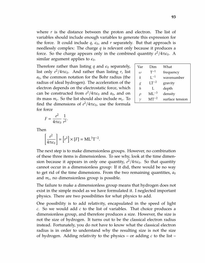
101 101

101 101

93

2010-05-13 00:43:32 / rev b667c9e4c1f1+

where r is the distance between the proton and electron. The list ofvariables should include enough variables to generate this expression forthe force. It could include q, ε0, and r separately. But that approach isneedlessly complex: The charge q is relevant only because it produces aforce. So the charge appears only in the combined quantity e2/4πε0. Asimilar argument applies to ε0.

Var Dim Whatω T−1 frequencyk L−1 wavenumberg LT−2 gravityh L depthρ ML−3 densityγ MT−2 surface tension

Therefore rather than listing q and ε0 separately,list only e2/4πε0. And rather than listing r, lista0, the common notation for the Bohr radius (theradius of ideal hydrogen). The acceleration of theelectron depends on the electrostatic force, whichcan be constructed from e2/4πε0 and a0, and onits mass me. So the list should also include me. Tofind the dimensions of e2/4πε0, use the formulafor force

F =e2

4πε0

1r2 .

Then[e2

4πε0

]=

[r2]× [F] = ML3T−2.

The next step is to make dimensionless groups. However, no combinationof these three items is dimensionless. To see why, look at the time dimen-sion because it appears in only one quantity, e2/4πε0. So that quantitycannot occur in a dimensionless group: If it did, there would be no wayto get rid of the time dimensions. From the two remaining quantities, a0and me, no dimensionless group is possible.

The failure to make a dimensionless group means that hydrogen does notexist in the simple model as we have formulated it. I neglected importantphysics. There are two possibilities for what physics to add.

One possibility is to add relativity, encapsulated in the speed of lightc. So we would add c to the list of variables. That choice produces adimensionless group, and therefore produces a size. However, the size isnot the size of hydrogen. It turns out to be the classical electron radiusinstead. Fortunately, you do not have to know what the classical electronradius is in order to understand why the resulting size is not the sizeof hydrogen. Adding relativity to the physics – or adding c to the list –

102 102

102 102

94

2010-05-13 00:43:32 / rev b667c9e4c1f1+

allows radiation. So the orbiting, accelerating electron would radiate. Asradiation carries energy away from the electron, it spirals into the proton,meaning that in this world hydrogen does not exist, nor do other atoms.

The other possibility is to add quantum mechanics, which was developedto solve fundamental problems like the existence of matter. The physics ofquantum mechanics is complicated, but its effect on dimensional analysesis simple: It contributes a new constant of nature ~ whose dimensions arethose of angular momentum. Angular momentum is mvr, so

[~] = ML2T−1.

Var Dim Whata0 L size

e2/4πε0 ML3T−2

me M electron mass~ ML2T−1 quantum

The ~ might save the day. There are nowtwo quantities containing time dimensions.Since e2/4πε0 has T−2 and ~ has T−1, the ra-tio ~2/(e2/4πε0) contains no time dimensions.Since[

~2

e2/4πε0

]= ML,

a dimensionless group is

~2

a0me(e2/4πε0)

It turns out that all dimensionless groups can be formed from this group.So, as in the spring–mass example, the only possible true statement in-volving this group is

~2

a0me(e2/4πε0)= dimensionless constant.

Therefore, the size of hydrogen is

a0 ∼~2

me(e2/4πε0).

Putting in values for the constants gives

a0 ∼ 0.5Å = 0.5 ·10−10 m.

It turns out that the missing dimensionless constant is 1: Dimensionalanalysis has given the exact answer.

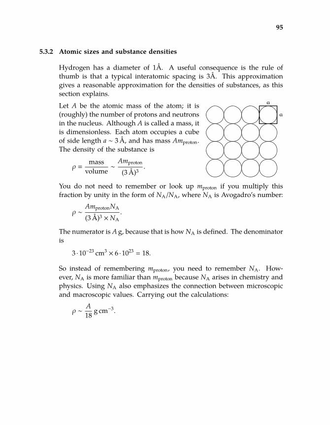
103 103

103 103

95

2010-05-13 00:43:32 / rev b667c9e4c1f1+

5.3.2 Atomic sizes and substance densities

Hydrogen has a diameter of 1Å. A useful consequence is the rule ofthumb is that a typical interatomic spacing is 3Å. This approximationgives a reasonable approximation for the densities of substances, as thissection explains.

a

aLet A be the atomic mass of the atom; it is(roughly) the number of protons and neutronsin the nucleus. Although A is called a mass, itis dimensionless. Each atom occupies a cubeof side length a ∼ 3Å, and has mass Amproton.The density of the substance is

ρ =mass

volume∼

Amproton

(3Å)3.

You do not need to remember or look up mproton if you multiply thisfraction by unity in the form of NA/NA, where NA is Avogadro’s number:

ρ ∼AmprotonNA

(3Å)3 ×NA.

The numerator is Ag, because that is how NA is defined. The denominatoris

3 ·10−23 cm3× 6 ·1023 = 18.

So instead of remembering mproton, you need to remember NA. How-ever, NA is more familiar than mproton because NA arises in chemistry andphysics. Using NA also emphasizes the connection between microscopicand macroscopic values. Carrying out the calculations:

ρ ∼A18

g cm−3.

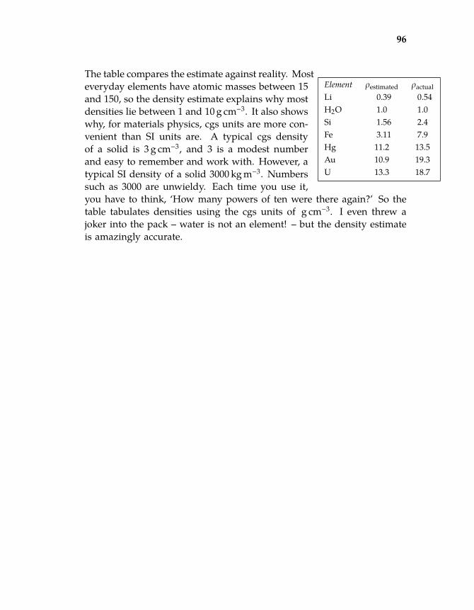
104 104

104 104

96

2010-05-13 00:43:32 / rev b667c9e4c1f1+

Element ρestimated ρactualLi 0.39 0.54H2O 1.0 1.0Si 1.56 2.4Fe 3.11 7.9Hg 11.2 13.5Au 10.9 19.3U 13.3 18.7

The table compares the estimate against reality. Mosteveryday elements have atomic masses between 15and 150, so the density estimate explains why mostdensities lie between 1 and 10g cm−3. It also showswhy, for materials physics, cgs units are more con-venient than SI units are. A typical cgs densityof a solid is 3g cm−3, and 3 is a modest numberand easy to remember and work with. However, atypical SI density of a solid 3000kgm−3. Numberssuch as 3000 are unwieldy. Each time you use it,you have to think, ‘How many powers of ten were there again?’ So thetable tabulates densities using the cgs units of g cm−3. I even threw ajoker into the pack – water is not an element! – but the density estimateis amazingly accurate.

105 105

105 105

97

2010-05-13 00:43:32 / rev b667c9e4c1f1+

5.4 Bending of light by gravity

Rocks, birds, and people feel the effect of gravity. So why not light?The analysis of that question is a triumph of Einstein’s theory of generalrelativity. We could calculate how gravity bends light by solving theso-called geodesic equations from general relativity:

d2xβ

dλ2 + Γβµν

dxµ

dλdxν

dλ= 0,

wwhere Γβµν are the Christoffel symbols, whose evaluation requires solv-

ing for the metric tensor gµν, whose evaluation requires solving the general-relativity curvature equations Rµν = 0.The curvature equations are themselves a shorthand for ten partial-differentialequations. The equations are rich in mathematical interest but are a night-mare to solve. The equations are numerous; worse, they are nonlinear.Therefore, the usual method for handling linear equations – guessing ageneral form for the solution and making new solutions by combininginstances of the general form – does not work. One can spend a decadelearning advanced mathematics to solve the equations exactly. Instead,apply a familiar principle: When the going gets tough, lower your stan-dards. By sacrificing some accuracy, we can explain light bending in fewerthan one thousand pages – using mathematics and physics that you (andI!) already know.The simpler method is dimensional analysis, in the usual three steps:

1. Find the relevant parameters.2. Find dimensionless groups.3. Use the groups to make the most general dimensionless statement.4. Add physical knowledge to narrow the possibilities.

These steps are done in the following sections.

5.4.1 Finding parameters

The first step in a dimensional analysis is to decide what physical para-meters the bending angle can depend on. For that purpose I often startwith an unlabeled diagram, for it prods me into thinking of labels; andmany of the labels are parameters of the problem.

106 106

106 106

98

2010-05-13 00:43:32 / rev b667c9e4c1f1+

sun

Here various parameters and reasons to include them:

1. The list has to include the quantity to solve for. So the angle θ is thefirst item in the list.

2. The mass of the sun, m, has to affect the angle. Black holes greatlydeflect light, probably because of their huge mass.

3. A faraway sun or black hole cannot strongly affect the path (near theearth light seems to travel straight, in spite of black holes all over theuniverse); therefore r, the distance from the center of the mass, is arelevant parameter. The phrase ‘distance from the center’ is ambigu-ous, since the light is at various distances from the center. Let r bethe distance of closest approach.

4. The dimensional analysis needs to know that gravity produces thebending. The parameters listed so far do not create any forces. Soinclude Newton’s gravitational constant G.

Here is the diagram with important parameters labeled:

sunmassm

θ

r

Here is a table of the parameters and their dimensions:Parameter Meaning Dimensionsθ angle –m mass of sun MG Newton’s constant L3T−2M−1

r distance from center of sun L

107 107

107 107

99

2010-05-13 00:43:32 / rev b667c9e4c1f1+

where L, M, and T represent the dimensions of length, mass, and time,respectively.

5.4.2 Dimensionless groups

The second step is to form dimensionless groups. One group is easy:The parameter θ is an angle, which is already dimensionless. The othervariables, G, m, and r, cannot form a second dimensionless group. To seewhy, following the dimensions of mass. It appears only in G and m, so adimensionless group would contain the product Gm, which has no massdimensions in it. But Gm and r cannot get rid of the time dimensions. Sothere is only one independent dimensionless group, for which θ is thesimplest choice.

Without a second dimensionless group, the analysis seems like nonsense.With only one dimensionless group, it must be a constant. In slowmotion:

θ = function of other dimensionless groups,

but there are no other dimensionless groups, so

θ = constant.

This conclusion is crazy! The angle must depend on at least one of mand r. Let’s therefore make another dimensionless group on which θ candepend. Therefore, return to Step 1: Finding parameters. The list lacks acrucial parameter.

What physics has been neglected? Free associating often suggests themissing parameter. Unlike rocks, light is difficult to deflect, otherwisehumanity would not have waited until the 1800s to study the deflection,whereas the path of rocks was studied at least as far back as Aristotleand probably for millions of years beforehand. Light travels much fasterthan rocks, which may explain why light is so difficult to deflect: Thegravitational field gets hold of it only for a short time. But none of theparameters distinguish between light and rocks. Therefore let’s includethe speed of light c. It introduces the fact that we are studying light, andit does so with a useful distinguishing parameter, the speed.

Here is the latest table of parameters and dimensions:

108 108

108 108

100

2010-05-13 00:43:32 / rev b667c9e4c1f1+

Parameter Meaning Dimensionsθ angle –m mass of sun MG Newton’s constant L3T−2M−1

r distance from center of sun Lc speed of light LT−1

Length is strewn all over the parameters (it’s in G, r, and c). Mass, how-ever, appears in only G and m, so the combination Gm cancels out mass.Time also appears in only two parameters: G and c. To cancel out time,form Gm/c2. This combination contains one length, so a dimensionlessgroup is Gm/rc2.

5.4.3 Drawing conclusions

The most general relation between the two dimensionless groups is

θ = f(Gm

rc2

).

Dimensional analysis cannot determine the function f , but it has told usthat f is a function only of Gm/rc2 and not of the variables separately.

Physical reasoning and symmetry narrow the possibilities. First, stronggravity – from a large G or m – should increase the angle. So f shouldbe an increasing function. Now apply symmetry. Imagine a world wheregravity is repulsive or, equivalently, where the gravitational constant isnegative. Then the bending angle should be negative; to make that hap-pen, f must be an odd function: namely, f (−x) = − f (x). This symmetryargument eliminates choices like f (x) ∼ x2.

The simplest guess is that f is the identity function: f (x) ∼ x. Then thebending angle is

θ =Gmrc2 .

But there is probably a dimensionless constant in f . For example,

θ = 7Gmrc2

and

109 109

109 109

101

2010-05-13 00:43:32 / rev b667c9e4c1f1+

θ = 0.3Gmrc2

are also possible. This freedom means that we should use a twiddlerather than an equals sign:

θ ∼Gmrc2 .

5.4.4 Comparison with exact calculations

All theories of gravity have the same form for the result, namely

θ ∼Gmrc2 .

The difference among the theories is in the value for the missing dimen-sionless constant:

θ =Gmrc2 ×

1 (simplest guess);2 (Newtonian gravity);4 (Einstein’s theory).

Here is a rough explanation of the origin of those constants. The 1 forthe simplest guess is just the simplest possible guess. The 2 for Newton-ian gravity is from integrating angular factors like cosine and sine thatdetermine the position of the photon as it moves toward and past the sun.The most interesting constant is the 4 for general relativity, which is dou-ble the Newtonian value. The fundamental reason for the factor of 2 isthat special relativity puts space and time on an equal footing to makespacetime. The theory of general relativity builds on special relativity byformulating gravity as curvature of spacetime. Newton’s theory is thelimit of general relativity that considers only time curvature; but gen-eral relativity also handles the space curvature. Most objects move muchslower than the speed of light, so they move much farther in time than inspace and see mostly the time curvature. For those objects, the Newton-ian analysis is fine. But light moves at the speed of light, and it thereforesees equal amounts of space and time curvature; so its trajectory bendstwice as much as the Newtonian theory predicts.

5.4.5 Numbers!

At the surface of the Earth, the dimensionless gravitational strength is

110 110

110 110

102

2010-05-13 00:43:32 / rev b667c9e4c1f1+

Gmrc2 ∼

6.7 ·10−11 m3 s−2 kg−1× 6.0 ·1024 kg

6.4 ·106 m × 3.0 ·108 ms−1 × 3.0 ·108 ms−1 ∼ 10−9.

This miniscule value is the bending angle (in radians). If physicists wantto show that light bends, they had better look beyond the earth! Thatstatement is based on another piece of dimensional analysis and physicalreasoning, whose result is quoted without proof: A telescope with mirrorof diameter d can resolve angles roughly as small as λ/d, where λ isthe wavelength of light; this result is based on the same physics as thediffraction pattern on a CDROM (Section 1.1). One way to measure thebending of light is to measure the change in position of the stars. A lensthat could resolve an angle of 10−9 has a diameter of at least

d ∼ λ/θ ∼ 0.5 ·10−6 m10−9 ∼ 500m.

Large lenses warp and crack; one of the largest existing lenses has d ∼ 6m.No practical mirror can have d ∼ 500m, and there is no chance of detectinga deflection angle of 10−9.

Physicists therefore searched for another source of light bending. In thesolar system, the largest mass is the sun. At the surface of the sun, thefield strength is

Gmrc2 ∼

6.7 ·10−11 m3 s−2 kg−1× 2.0 ·1030 kg

7.0 ·108 m × 3.0 ·108 ms−1 × 3.0 ·108 ms−1 ∼ 2.1 ·10−6≈ 0.4′′.

This angle, though small, is possible to detect: The required lens diameteris roughly

d ∼ λ/θ ∼ 0.5 ·10−6 m2.1 ·10−6 ∼ 20 cm.

The eclipse expedition of 1919, led by Arthur Eddington of CambridgeUniversity, tried to measure exactly this effect.

For many years – between 1909 and 1916 – Einstein believed that a correcttheory of gravity would predict the Newtonian value, which turns out tobe 0.87 arcseconds for light that grazes the surface of the sun. The Germanmathematician Soldner derived the same result in 1803. Fortunately forEinstein’s reputation, the eclipse expeditions that went to test his (andSoldner’s) prediction got rained or clouded out. By the time an expeditiongot lucky with the weather (Eddington’s in 1919), Einstein had invented

111 111

111 111

103

2010-05-13 00:43:32 / rev b667c9e4c1f1+

a new theory of gravity – general relativity – and it predicted a deflectionof 1.75 arcseconds.

The goal of Eddington’s expedition was to decide between the Newtonianand general relativity values. The measurements are difficult, and theresults were not accurate enough to decide which theory was right. But1919 was the first year after the World War in which Germany and Britainhad fought each other almost to oblivion. A theory invented by a German,confirmed by an Englishman (from Newton’s university, no less) – sucha picture was comforting after the trauma of war. The world press andscientific community saw what they wanted to: Einstein vindicated!

A proper confirmation of Einstein’s prediction came only with the ad-vent of radio astronomy, in whichsmall deflections could be measuredaccurately. Here is then a puzzle: If the accuracy (resolving power) ofa telescope is λ/d, where λ is the wavelength and d is the telescope’sdiamater, how could radio telescopes be more accurate than optical ones,since radio waves have a much longer wavelength than light?

112 112

112 112

104

2010-05-13 00:43:32 / rev b667c9e4c1f1+

5.5 Buckingham Pi theorem

The second step is in a dimensional analysis is to make dimensionlessgroups. That task is simpler by knowing in advance how many groupsto look for. The Buckingham Pi theorem provides that number. I deriveit with a series of examples.

Here is a possible beginning of the theorem statement: The number ofdimensionless groups is. . . . Try it on the light-bending example. Howmany groups can the variables θ, G, m, r, and c produce? The possibilitiesinclude θ, θ2, Gm/rc2, θGm/rc2, and so on. The possibilities are infinite!Now apply the theorem statement to estimating the size of hydrogen,before including quantum mechanics in the list of variables. That list isa0 (the size), e2/4πε0, and me. That list produces no dimensionless groups.So it seems that the number of groups would be zero – if no groups arepossible – or infinity, if even one group is possible.

Here is an improved theorem statement taking account of the redundancy:The number of independent dimensionless groups is. . . . To complete thestatement, try a few examples:

1. Bending of light. The five quantities θ, G, m, r, and c produce twoindependent groups. A convenient choice for the two groups is θ andGm/rc2, but any other independent set is equally valid, even if not asintuitive.

2. Size of hydrogen without quantum mechanics. The three quantitiesa0 (the size), e2/4πε0, and me produce zero groups.

3. Size of hydrogen with quantum mechanics. The four quantities a0 (thesize), e2/4πε0, me, and ~ produce one independent group.

These examples fit a simple pattern:

no. of independent groups = no. of quantities − 3.

The 3 is a bit distressing because it is a magic number with no explanation.It is also the number of basic dimensions: length, mass, and time. Soperhaps the statement is

no. of independent groups = no. of quantities − no. of dimensions.

Test this statement with additional examples:

113 113

113 113

105

2010-05-13 00:43:32 / rev b667c9e4c1f1+

1. Period of a spring–mass system. The quantities are T (the period), k, m,and x0 (the amplitude). These four quantities form one independentdimensionless group, which could be kT2/m. This result is consistentwith the proposed theorem.

2. Period of a spring–mass system (without x0). Since the amplitudex0 does not affect the period, the quantities could have been T (theperiod), k, and m. These three quantities form one independent di-mensionless group, which again could be kT2/m. This result is alsoconsistent with the proposed theorem, since T, k, and m contain onlytwo dimensions (mass and time).

The theorem is safe until we try to derive Newton’s second law. The forceF depends on mass m and acceleration a. Those three quantities containthree dimensions – mass, length, and time. Three minus three is zero, sothe proposed theorem predicts zero independent dimensionless groups.Whereas F = ma tells me that F/ma is a dimensionless group.

Var Dim WhatF MLT−2 forcem M massa LT−2 acceleration

This problem can be fixed by adding one word tothe statement. Look at the dimensions of F, m, anda. All the dimensions – M or MLT−2 or LT−2 – canbe constructed from only two dimensions: M andLT−2. The key idea is that the original set of threedimensions are not independent, whereas the pairM and LT−2 are independent. So:

# of independent groups = # of quantities−# of independent dimensions.

That statement is the Buckingham Pi theorem [3].

5.6 Drag

For the final example of dimensional analysis, we revisit the cone exper-iment of Section 3.3.1. That analysis, using conservation, concluded thatthe drag force on the cones is given by

Fdrag ∼ ρv2A, (5.1)

where ρ is the density of the fluid (e.g. air or water), v is the speed of thecone, and A is its cross-sectional area. What can dimensional analysis tellus about this problem?

114 114

114 114

106

2010-05-13 00:43:32 / rev b667c9e4c1f1+

The strategy is to find the quantities that affect Fdrag, find their dimen-sions, and then find dimensionless groups.

On what quantities does the drag depend, and what are their dimensions?

v speed of the cone LT−1

r size of the cone L

ρ density of air ML−3

ν viscosity of air L2T−1

The drag force depends on four quan-tities: two parameters of the cone andtwo parameters of the fluid (air). Anydimensionless form can be built from di-mensionless groups: from dimensionlessproducts of the variables. Because anyequation describing the world can be written in a dimensionless form,and any dimensionless form can be written using dimensionless groups,any equation describing the world can be written using dimensionlessgroups.

Problem 5.3 Kepler’s third lawUse dimensional analysis to derive Kepler’s third law connecting the orbitalperiod of a planet to its orbital radius (for a circular orbit).

What dimensionless groups can be constructed for the drag problem?

According to the Buckingham Pi theorem, the five quantities and three in-dependent dimensions give rise to two independent dimensionless groups.One dimensionless group could be F/ρv2r2. A second group could berv/ν. Any other dimensionless group can be constructed from these twogroups (Problem 5.4), so the problem is indeed described by two indepen-dent dimensionless groups. The most general dimensionless statement isthen

one group = f (second group), (5.2)

where f is a still-unknown (but dimensionless) function.

Which dimensionless group belongs on the left side?

The goal is to synthesize a formula for F, and F appears only in the firstgroup F/ρv2r2. With that constraint in mind, place the first group on theleft side rather than wrapping it in the still-mysterious function f . Withthis choice, the most general statement about drag force is

115 115

115 115

107

2010-05-13 00:43:32 / rev b667c9e4c1f1+

Fρv2r2 = f

(rvν

). (5.3)

The physics of the (steady-state) drag force on the cone is all contained inthe dimensionless function f . However, dimensional analysis cannot tellus anything about that function. To make progress requires incorporatingnew knowledge. It can come from an experiment such as dropping thesmall and large cones, from wind-tunnel tests at various speeds, and evenfrom physical reasoning.

Before reexamining the results of the cone experiment in dimensionlessform, let’s name the two dimensionless groups. The first one, F/ρv2r2, istraditionally written in a slightly different form:

F12ρv2A

, (5.4)

where A is the cross-sectional area of the cone. The 1/2 is an arbitrarychoice, but it is the usual choice: It is convenient and is reminiscent ofthe 1/2 in the kinetic energy formula mv2/2. Written in that way, the firstdimensionless group is called the drag coefficient and is abbreviated cd.The second group, rv/ν, is called the Reynolds number. It is traditionallywritten in terms of the diameter rather than the radius:

vLν, (5.5)

where L is the diameter of the object.

The conclusion of the dimensional analysis is then

drag coefficient = f (Reynolds number). (5.6)

Now let’s see how the cone experiment fits into this dimensionless frame-work. The experimental data was that the small and large cones fell atthe same speed – roughly 1ms−1. The conclusion is that the drag forceis proportional to the cross-sectional area A. Because the drag coefficientis proportional to F/A, which is the same for the small and large cones,the small and large cones have the same drag coefficient.

Their Reynolds numbers, however, are not the same. For the small cone,the diameter is 2 in × 0.75 (why?), which is roughly 4 cm. The Reynoldsnumber is

116 116

116 116

108

2010-05-13 00:43:32 / rev b667c9e4c1f1+

Re ∼ 1ms−1× 0.04m

1.5 ·10−5 m2 s−1 , (5.7)

where 1ms−1 is the fall speed and 1.5·10−5 m2 s−1 is the kinematic viscosityof air. Numerically, Resmall ∼ 2000. For the large cone, the fall speedand viscosity are the same as for the small cone, but the diameter istwice as large, so Relarge ∼ 4000. The result of the cone experiment is, indimensionless form, that the drag coefficient is independent of Reynoldsnumber – at least, for Reynolds numbers between 2000 and 4000.

This conclusion is valid for diverse shapes. The most extensive data ondrag coefficient versus Reynolds number is for a sphere. That data is plot-ted logarithmically below (from Fluid-dynamic Drag: Practical Informationon Aerodynamic Drag and Hydrodynamic Resistance by Sighard F. Hoerner):

Just like the cones, the sphere’s drag coefficient is almost constant in theReynolds number range 2000 to 4000. This full graph has interesting fea-tures. First, toward the low-Reynolds-number end, the drag coefficientincreases. Second, for high Reynolds numbers, the drag coefficient staysroughly constant until Re ∼ 106, where it rapidly drops by almost a factorof 5. The behavior at low Reynolds number will be explained in the chap-ter on easy (extreme) cases (Chapter 6). The drop in the drag coefficient,which relates to why golf balls have dimples, will be explained in thechapter on lumping (Chapter 7).

117 117

117 117

109

2010-05-13 00:43:32 / rev b667c9e4c1f1+

Problem 5.4 Only two groupsShow that F, v, r, ρ, and ν produce only two independent dimensionless groups.

Problem 5.5 Counting dimensionless groupsHow many independent dimensionless groups are there in the following sets ofvariables:

a. size of hydrogen including relativistic effects:

e2/4πε0, ~, c, a0 (Bohr radius), me (electron mass).

b. period of a spring–mass system in a gravitational field:

T (period), k (spring constant), m, x0 (amplitude), g.

c. speed at which a free-falling object hits the ground:

v, g, h (initial drop height).

d. [tricky!] weight W of an object:

W, g, m.

Problem 5.6 Integrals by dimensionsYou can use dimensions to do integrals. As an example, try this integral:

I(β) =

∫∞

−∞

e−βx2dx.

Which choice has correct dimensions: (a.)√πβ−1 (b.)

√πβ−1/2 (c.)

√πβ1/2

(d.)√πβ1

Hints:

1. The dimensions of dx are the same as the dimensions of x.

2. Pick interesting dimensions for x, such as length. (If x is dimensionless thenyou cannot use dimensional analysis on the integral.)

Problem 5.7 How to avoid remembering lots of constantsMany atomic problems, such as the size or binding energy of hydrogen, end upin expressions with ~, the electron mass me, and e2/4πε0, which is a nicer way toexpress the squared electron charge. You can avoid having to remember thoseconstants if instead you remember these values instead:

~c ≈ 200 eVnm = 2000 eVÅmec2

∼ 0.5 ·106 eVe2/4πε0~c

≡ α ≈1

137(fine-structure constant).

118 118

118 118

110

2010-05-13 00:43:32 / rev b667c9e4c1f1+

Use those values to evaluate the Bohr radius in angstroms (1Å = 0.1nm):

a0 =~2

me(e2/4πε0).

As an example calculation using the ~c value, here is the energy of a photon:

E = h f = 2π~ f = 2π~ cλ,

where f is its frequency and λ is its wavelength. For green light, λ ∼ 600nm, so

E ∼

2π︷︸︸︷6 ×

~c︷ ︸︸ ︷200 eVnm

600nm︸ ︷︷ ︸λ

∼ 2 eV.

Problem 5.8 Heavy nucleiIn lecture we analyzed hydrogen, which is one electron bound to one proton. Inthis problem you study the innermost electron in an atom such as uranium thathas many protons, and analyze one physical consequence of its binding energy.

So, imagine a nucleus with Z protons around which orbits one electron. LetE(Z) be the binding energy (the hydrogen energy is the case Z = 1).

a. Show that the ratio E(Z)/E(1) is Z2.

b. In lecture, we derived that E(1) is the kinetic energy of an electron movingwith speed αc where α is the fine-structure constant (roughly 10−2). Howfast does the innermost electron move around a heavy nucleus with chargeZ?

c. When that speed is comparable to the speed of light, the electron has a kineticenergy comparable to its (relativistic) rest energy. One consequence of such ahigh kinetic energy is that the electron has enough kinetic energy to producea positron (an anti-electron) out of nowhere (‘pair creation’). That positronleaves the nucleus, turning a proton into a neutron as it exits. So the atomicnumber Z drops by one: The nucleus is unstable! Relativity sets an upperlimit for Z.

Estimate that maximum Z and compare it with the Z for the heaviest stablenucleus (uranium).

Problem 5.9 Power radiated by an accelerating chargeElectromagnetism, where the usual derivations are so cumbersome, is an excel-lent area to apply dimensional analysis. In this problem you work out the powerradiated by an accelerating charge, which is how radio stations work.

So, consider a particle with charge q, with position x, velocity v, and accelerationa. What variables are relevant to the radiated power P? The position cannot

119 119

119 119

111

2010-05-13 00:43:32 / rev b667c9e4c1f1+

matter because it depends on the origin of the coordinate system, whereas thepower radiated cannot depend on the origin. The velocity cannot matter becauseof relativity: You can transform to a reference frame where v = 0, but that changewill not affect the radiation (otherwise you could distinguish a moving framefrom a non-moving frame, in violation of the principle of relativity). So theacceleration a is all that’s left to determine the radiated power. [This line ofargument is slightly dodgy, but it works for low speeds.]

a. Using P, q2/4πε0, and a, how many dimensionless quantities can you form?

b. Fix the problem in the previous part by adding one quantity to the list ofvariables, and give a physical reason for including the quantity.

c. With the new list, use dimensionless groups to find the power radiated by anaccelerating point charge. In case you are curious, the exact result containsa dimensionless factor of 2/3; dimensional analysis triumphs again!

Problem 5.10 Yield from an atomic bombGeoffrey Taylor, a famous Cambridge fluid mechanic, annoyed the US govern-ment by doing the following analysis. The question he answered: ‘What wasthe yield (in kilotons of TNT) of the first atomic blast (in the New Mexico desertin 1945)?’ Declassified pictures, which even had a scale bar, gave the followingdata on the radius of the explosion at various times:

t (ms) R (m)3.26 59.04.61 67.3

15.0 106.562.0 185.0

a. Use dimensional analysis to work out the relation between radius R, time t,blast energy E, and air density ρ.

b. Use the data in the table to estimate the blast energy E (in Joules).

c. Convert that energy to kilotons of TNT. One gram of TNT releases 1kcal orroughly 4kJ.

The actual value was 20kilotons, a classified number when Taylor publishedhis result [‘The Formation of a Blast Wave by a Very Intense Explosion. II. TheAtomic Explosion of 1945.’, Proceedings of the Royal Society of London. Series A,Mathematical and Physical 201(1065): 175–186 (22 March 1950)]

120 120

120 120

112

2010-05-13 00:43:32 / rev b667c9e4c1f1+

Problem 5.11 Atomic blast: A physical interpretationUse energy densities and sound speeds to make a rough physical explanation ofthe result in the ‘yield from an atomic bomb’ problem.

Problem 5.12 Rolling down the planeFour objects, made of identical steel, roll down an inclined plane without slip-ping. The objects are:

1. a large spherical shell,2. a large disc,3. a small solid sphere,4. a small ring.

The large objects have three times the radius of the small objects. Rank theobjects by their acceleration (highest acceleration first).

Check your results with exact calculation or with a home experiment.

Problem 5.13 Blackbody radiation

A hot object – a so-called blackbody – radiates energy, and the flux F depends onthe temperature T. In this problem you derive the connection using dimensionalanalysis. The goal is to find F as a function of T. But you need more quantities.

a. What are the dimensions of flux?

b. What two constants of nature should be included because blackbody radia-tion depends on the quantum theory of radiation?

c. What constant of nature should be included because you are dealing withtemperature?

d. After doing the preceding parts, you have five variables. Explain why thesefive variables produce one dimensionless group, and use that fact to deducethe relation between flux and temperature.

e. Look up the Stefan–Boltzmann law and compare your result to it.

121 121

121 121

113

2010-05-13 00:43:32 / rev b667c9e4c1f1+

Part 3

Lossycompression

6 Easy cases 115

7 Lumping 133

8 Probabilistic reasoning 151

9 Springs 175

122 122

122 1222010-05-13 00:43:32 / rev b667c9e4c1f1+

123 123

123 1232010-05-13 00:43:32 / rev b667c9e4c1f1+

6Easy cases

6.1 Pyramid volume 1156.2 Atwood machine 1176.3 Drag 120

The previous tools included methods for organizing complexity and meth-ods for losslessly discarding complexity (for example, dimensional analy-sis). However, the world often throws us problems so complex – forexample, almost any question in fluid mechanics – that these methodsare insufficient on their own. Therefore, we now start to study meth-ods for discarding actual complexity. With these methods, we accept areduction in accuracy in order to reach a solution at all.

The first tool for discarding actual complexity is based on the principlethat a correct solution works in all cases – including the easy ones. Thisprinciple helps us check and, more surprisingly, helps us guess solutions.

6.1 Pyramid volume

As the first example, let’s explain the factor of one-third in the volume ofa pyramid with a square base:

V =13

hb2,

where h is the altitude and b is the length of a side of the base.

124 124

124 124

116

2010-05-13 00:43:32 / rev b667c9e4c1f1+

b

h = b

Rather than explaining right away the one-third inthe volume of a pyramid, a difficult three-dimensionalproblem, let’s first find the corresponding constantin a two-dimensional problem. That problem is thearea of a triangle with base b and height h; its area isA ∼ bh. What is the constant? Choose a convenienttriangle – a special, easy case – perhaps a 45-degree right triangle whereh = b. Two such triangles form a square with area b2, so A = b2/2 whenh = b. The constant in A ∼ bh is therefore 1/2 no matter what b and h are,so A = bh/2.

Now use the same construction in three dimensions.What square-based pyramid, when combined with it-self perhaps several times, makes a familiar shape? Inother words, find an easy case of h and b, and makesure that the volume is correct in that case. Becauseonly the aspect ratio h/b matters in the following dis-cussion, choose b conveniently, then choose h to makea pyramid with the right aspect ratio. The goal shapeis suggested by the square pyramid base. One easysolid with a square base is a cube.

Therefore, let’s try to combine several pyramids into a cube of side b. Tosimplify the upcoming arithmetic, I choose b = 2. What should the heighth be? To decide, imagine how the cube will be constructed. Each cube hassix faces, so six pyramids might make a cube where each pyramid baseforms one face of the cube, and each pyramid tip faces inward, meetingin the center of the cube. For the tips to meet in the center of the cube,the height must be h = 1. So six pyramids with b = 2, and h = 1 make acube with side length 2.

The volume of one pyramid is one-sixth of the volume of this cube:

V =cube volume

6=

86

=43.

The volume of the pyramid is V ∼ hb2, and the missing constant mustmake volume 4/3. Since hb2 = 4 for these pyramids, the missing constantis 1/3. Voilà:

V =13

hb2.

125 125

125 125

117

2010-05-13 00:43:32 / rev b667c9e4c1f1+

6.2 Atwood machine

m1

m2

The next problem illustrates dimensional analysis and easycases in a physical problem. The problem is the Atwood ma-chine, a staple of the first-year physics curriculum. Twomasses,m1 and m2, are connected and, thanks to a pulley, are free tomove up and down. What is the acceleration of the massesand the tension in the string? You can solve this problem withstandard methods from first-year physics, which means thatyou can can check the solution that we derive using dimensional analy-sis, easy cases, and a feel for functions.

The first problem is to find the acceleration of, say, m1. Since m1 and m2are connected by a rope, the acceleration of m2 is, depending on your signconvention, either equal to m1 or equal to −m1. Let’s call the accelerationa and use dimensional analysis to guess its form. The first step is todecide what variables are relevant. The acceleration depends on gravity,so g should be on the list. The masses affect the acceleration, so m1 andm2 are on the list. And that’s it. You might wonder what happened tothe tension: Doesn’t it affect the acceleration? It does, but it is itself aconsequence of m1, m2, and g. So adding tension to the list does not addinformation; it would instead make the dimensional analysis difficult.

Var Dim Whata LT−2 accel. of m1g LT−2 gravity

m1 M block massm2 M block mass

These variables fall into two pairs where the vari-ables in each pair have the same dimensions. So thereare two dimensionless groups here ripe for picking:G1 = m1/m2 and G2 = a/g. You can make any dimen-sionless group using these two obvious groups, asexperimentation will convince you. Then, followingthe usual pattern,

ag

= f(m1

m2

),

where f is a dimensionless function.

Pause a moment. The more thinking that you do to choose a clean rep-resentation, the less algebra you do later. So rather than find f usingm1/m2 as the dimensionless group, first choose a better group. The ratiom1/m2 does not respect the symmetry of the problem in that only thesign of the acceleration changes when you interchange the labels m1 andm2. Whereas m1/m2 turns into its reciprocal. So the function f will have

126 126

126 126

118

2010-05-13 00:43:32 / rev b667c9e4c1f1+

to do lots of work to turn the unsymmetric ratio m1/m2 into a symmetricacceleration.

Back to the drawing board for how to fix G1. Another option is to usem1 − m2. Wait, the difference is not dimensionless! I fix that problem ina moment. For now observe the virtue of m1 −m2. It shows a physicallyreasonable symmetry under mass interchange: G1 → −G1. To make itdimensionless, divide it by another mass. One candidate is m1:

G1 =m1 + m2

m1.

That choice, like dividing by m2, abandons the beloved symmetry. Butdividing by m1 + m2 solves all the problems:

G1 =m1 −m2

m1 + m2.

This group is dimensionless and it respects the symmetry of the problem.

Using this G1, the solution becomesag

= f(m1 −m2

m1 + m2

),

where f is another dimensionless function.

m1

To guess f (x), where x = G1, try the easy cases. First imagine thatm1 becomes huge. A quantity with mass cannot be huge on itsown, however. Here huge means huge relative to m2, whereuponx ≈ 1. In this thought experiment, m1 falls as if there were nom2 so a = −g. Here we’ve chosen a sign convention with positiveacceleration being upward. If m2 is huge relative to m1, whichmeans x = −1, then m2 falls like a stone pulling m1 upward withacceleration a = g. A third limiting case is m1 = m2 or x = 0, whereuponthe masses are in equilibrium so a = 0.

Here is a plot of our knowledge of f :

127 127

127 127

119

2010-05-13 00:43:32 / rev b667c9e4c1f1+

x

f(x)

1-1

1

-1

The simplest conjecture – an educated guess – is that f (x) = x. Then wehave our result:

ag

=m1 −m2

m1 + m2.

Look how simple the result is when derived in a symmetric, dimension-less form using easy cases.

128 128

128 128

120

2010-05-13 00:43:32 / rev b667c9e4c1f1+

6.3 Drag

Although the method of easy cases is a lossy method – it throws awayinformation – it gave us exact results in the preceding examples. Let’ssharpen the easy-cases tool by applying it to that favorite difficult prob-lem: drag. The conclusion of dimensional analysis was

drag coefficient = f (Reynolds number). (6.1)

The remaining problem, which dimensional analysis could not solve, isto find the function f .

One approach to finding f is experimental. Drop cones of different sizes,use the geometry and terminal velocity to compute the drag coefficientand Reynolds number, and plot the results. We used this approach withtwo cones, finding that the drag coefficient was the same at a Reynoldsnumber of 2000 and 4000. These two data points are only over a limitedrange of Reynolds number. What happens in other cases, for examplewhen the Reynolds number is 0.1 or 106?

Such experiments would provide the most accurate map of f . However,these experiments are difficult, and they do not help us understand whyf has the shape that it has. To that end, we use physical reasoning usingthe method of easy cases. When we applied easy cases to the pyramid,we chose h and b to make an easy pyramid (one that could be replicatedand combined into a square). For drag, we choose the Reynolds numberto simplify the physical reasoning. One choice is the regime of largeReynolds numbers: Re 1 (the two falling cones are examples). Thephysical reasoning in this regime is the subject of Section 6.3.1. The othereasy case is the regime of low Reynolds numbers: Re 1 (Section 6.3.2).

6.3.1 Turbulent limit

When the Reynolds number is high – for example, at very high speeds– the flow becomes turbulent. The high-Reynolds-number limit can bereached many ways. One way is to shrink the viscosity ν to 0, because νlives in the denominator of the Reynolds number. Therefore, in the limitof high Reynolds number, viscosity disappears from the problem andthe drag force should not depend on viscosity. This reasoning containsseveral subtle untruths, yet its conclusion is mostly correct. (Clarifying the

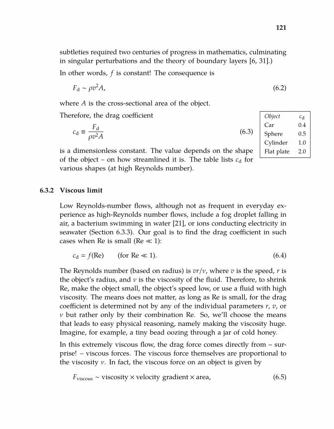
129 129

129 129

121

2010-05-13 00:43:32 / rev b667c9e4c1f1+

subtleties required two centuries of progress in mathematics, culminatingin singular perturbations and the theory of boundary layers [6, 31].)

In other words, f is constant! The consequence is

Fd ∼ ρv2A, (6.2)

where A is the cross-sectional area of the object.

Object cdCar 0.4Sphere 0.5Cylinder 1.0Flat plate 2.0

Therefore, the drag coefficient

cd ≡Fd

ρv2A(6.3)

is a dimensionless constant. The value depends on the shapeof the object – on how streamlined it is. The table lists cd forvarious shapes (at high Reynolds number).

6.3.2 Viscous limit

Low Reynolds-number flows, although not as frequent in everyday ex-perience as high-Reynolds number flows, include a fog droplet falling inair, a bacterium swimming in water [21], or ions conducting electricity inseawater (Section 6.3.3). Our goal is to find the drag coefficient in suchcases when Re is small (Re 1):

cd = f (Re) (for Re 1). (6.4)

The Reynolds number (based on radius) is vr/ν, where v is the speed, r isthe object’s radius, and ν is the viscosity of the fluid. Therefore, to shrinkRe, make the object small, the object’s speed low, or use a fluid with highviscosity. The means does not matter, as long as Re is small, for the dragcoefficient is determined not by any of the individual parameters r, v, orν but rather only by their combination Re. So, we’ll choose the meansthat leads to easy physical reasoning, namely making the viscosity huge.Imagine, for example, a tiny bead oozing through a jar of cold honey.

In this extremely viscous flow, the drag force comes directly from – sur-prise! – viscous forces. The viscous force themselves are proportional tothe viscosity ν. In fact, the viscous force on an object is given by

Fviscous ∼ viscosity × velocity gradient × area, (6.5)

130 130

130 130

122

2010-05-13 00:43:32 / rev b667c9e4c1f1+

where velocity gradient is the rate of change of velocity with distance(so if the velocity does not vary, then there is no viscous force), and thearea is the surface area of the object. Because the drag is due directly toviscous forces, the drag force is also proportional to viscosity:

Fd ∝ ν.

This constraint is sufficient to determine the form of the function f andtherefore to determine the drag force. Start with the result from dimen-sional analysis:

Fd

ρflr2v2 = f(vrν

).

The viscosity ν appears only in the Reynolds number, where it appearsin the denominator. To make Fd proportional to ν requires making thedrag coefficient proportional to Re−1. Equivalently, the function f , whenRe 1, is given by f (x) ∼ 1/x. For the drag force itself, the consequenceis

Fd ∼ ρflr2v2 νvr

= ρflνv.

Dimensional analysis alone is insufficient to compute the missing magicdimensionless constant. A fluid mechanic must do a messy and difficultcalculation that is possible only for a few special shapes. For a sphere,the British mathematician Stokes showed that the missing constant is 6π;in other words,

Fd = 6πρflνvr.

This result is called Stokes drag. In the next section, we will use thisresult to study electrical properties of seawater.

131 131

131 131

123

2010-05-13 00:43:32 / rev b667c9e4c1f1+

6.3.3 Conductivity of seawater

σ =1

ρ

ρ

R =V

Iblock geometry

V = El I = qnvA

E l n v A

Fq Fd

To illustrate a rare example of a situa-tion with low Reynolds numbers, we es-timate the electrical conductivity of sea-water. Doing this estimate requires di-viding and conquering.

The first question is: What is conduc-tivity? Conductivity σ is the recipro-cal of resistivity ρ. (Apologies for thesymbolic convention that overloads thedensity symbol with yet another mean-ing.) Resistivity is related to resistanceR. Then why have both ρ and R? Resis-tance is a useful measure for a particu-lar wire or resistor with a fixed size and shape. However, for a generalwire, the resistance depends on the wire’s length and cross-sectional area.In other words, resistance is not an intensive quantity. (It’s also not anextensive quantity, but that’s a separate problem.) Before determining therelationship between resistivity and resistance, let’s finish sketching thesolution tree, for now leaving ρ as depending on R plus geometry.

The second question is: What is a physical model for the resistance (andhow to measure it)? We can find R by placing a voltage V – and thereforean electric field – across a block of seawater and measuring the currentI. The resistance is given by R = V/I. But how does seawater conductelectricity? Conduction requires the transport of charge. Seawater ismostly water and table salt (NaCl). The ions that arise from dissolvingsalt transport charge. The resulting current is

I = qnvA,

where A is the cross-sectional area of the block, q is the ion charge, n isconcentration of the ion (ions per volume), and v is its terminal speed.

To understand and therefore rederive this formula, first check its dimen-sions. The left side, current, is charge per time. Is the right side alsocharge per time? Do it piece by piece: q is charge, and nvA has dimen-sions of T−1, so qnvA has dimensions of charge per time or current.

132 132

132 132

124

2010-05-13 00:43:32 / rev b667c9e4c1f1+

As a second check, watch a cross-section of the block for a time ∆t andcalculate how much charge flows during that time. The charges moveat speed v, so all charges in a rectangular block of width v∆t and areaA cross the cross-section. This rectangular block has volume vA∆t. Theion concentration is n, so the block contains nvA∆t charges. If each ionhas charge q, then the total charge on the ions is Q = qnvA∆t. It took atime ∆t for this charge to make its journey, so the current is, once again,I = Q/∆t = qnvA.

The drift speed v depends on the applied force Fq and on the drag forceFd. The ion adjusts its speed until the drag force matches the appliedforce. The result of this subdividing is the preceding map.

A

l

Now let’s find expressions for the unknown nodes.Only three remain: ρ, v, and n. The figure illus-trates the relation between ρ and R:

ρ =RAl.

To find v, we balance the drag and electrical forces. The applied force isFq = qE, where q is the ion charge and E is the electric field. The electricfield produced by the voltage V is E = V/l, where l is the length of theblock, so

Fq =qVl.

This expression contains no unknown quantities, so it does not need fur-ther subdivision.

The drag is Stokes drag:

Fd = 6πρflνvr. (6.6)

Equating this force to the applied force gives the terminal velocity v interms of known quantities:

v ∼qV

6πηlr,

where r is the radius of the ion.

The number density n is the third and final unknown. However, let’sestimate it after getting a symbolic result for σ. (This symbolic result will

133 133

133 133

125

2010-05-13 00:43:32 / rev b667c9e4c1f1+

contain n.) To find σ climb the solution tree. First, find the current interms of the terminal velocity:

I = qnvA ∼q2nAV6πηlr

.

Use the current to find the resistance:

R ∼ VI∼

6πηlrq2nA

.

The voltage V has vanished, which is encouraging: In most circuits, theconductivity (and resistance) is independent of voltage. Use the resistanceto find the resistivity:

ρ = RAl∼

6πηrq2n

.

The expressions simplify as we climb the tree. For example, the geometricparameters l and A have vanished. Their disappearance is encouraging –the purpose of evaluating resistivity rather than resistance is that resis-tivity is independent of geometry.

Now use resistivity to find conductivity:

σ =1ρ∼

q2n6πηr

.

Here q is the electron charge e or its negative, depending on whether asodium or a chloride ion is the charge carrier. Thus,

σ =1ρ∼

e2n6πηr

.

To find σ still requires the ion concentration n, which we can find from theconcentration of salt in seawater. To do so, try a kitchen-sink experiment.Add table salt to a glass of water until it tastes as salty as seawater. I justtried it. In a glass of water, I found that one teaspoon of salt tastes likedrinking seawater. A glass of water may have a volume of 0.3 ` or a massof 300g. A flat teaspoon of salt has a volume of about 5 m`. Why 5 m`?A teaspoon is about 4 cm long by 2 cm wide by 1 cm thick at its deepestpoint; let’s assume 0.5 cm on average. Its volume is therefore

teaspoon ∼ 4 cm × 2 cm × 0.5 cm ∼ 4 cm3.

134 134

134 134

126

2010-05-13 00:43:32 / rev b667c9e4c1f1+

The density of salt is maybe twice the density of water, so a flat teaspoonhas a mass of roughly 10g. The mass fraction of salt in seawater is, inthis experiment, roughly 1/30. The true value is remarkably close: 0.035.A mole of salt, which provides two charges per NaCl ‘molecule’, has amass of 60g, so

n ∼ 130× 1g cm−3︸ ︷︷ ︸

ρwater

×2 chargesmolecule

×6 ·1023 moleculesmole−1

60gmole−1

∼ 7 ·1020 charges cm−3.

With n evaluated, the only remaining mysteries in the conductivity

σ =1ρ∼

q2n6πηr

are the ion radius r and the dynamic viscosity η.

Do the easy part first. The dynamic viscosity is

η = ρwaterν ∼ 103 kgm−3× 10−6 m2 s−1 = 10−3 kgm−1 s−1.

Here I switched to SI (mks) units. Although most calculations are eas-ier in cgs units than in SI units, the one exception is electromagnetism,which is represented by the e2 in the conductivity. Electromagnetism isconceptually easier in cgs units – which needs no factors of µ0 or 4πε0, forexample – than in SI units. However, the cgs unit of charge, the electrosta-tic unit, is unfamiliar. So, for numerical calculations in electromagnetism,use SI units.

water

water

water

water

The final quantity required is the ion radius.A positive ion (sodium) attracts an oxygen endof a water molecule; a negative ion (chloride)attracts the hydrogen end of a water mole-cule. Either way, the ion, being charged, issurrounded by one or maybe more layers ofwater molecules. As it moves, it drags someof this baggage with it. So rather than usethe bare ion radius you should use a largerradius to include this shell. But how thick isthe shell? As a guess, assume that the shell includes one layer of watermolecules, each with a radius of 1.5Å. So for the ion plus shell, r ∼ 2Å.

135 135

135 135

127

2010-05-13 00:43:32 / rev b667c9e4c1f1+

With these numbers, the conductivity becomes:

σ ∼

e2︷ ︸︸ ︷(1.6 ·10−19 C)2

×

n︷ ︸︸ ︷7 ·1026 m−3

6 × 3︸︷︷︸6π

× 10−3 kgm−1 s−1︸ ︷︷ ︸η

× 2 ·10−10 m︸ ︷︷ ︸r

.

You can do the computation mentally. First count the powers of ten andthen worrying about the small factors. Then count the top and bottomcontributions separately. The top contributes −12 powers of 10: −38 frome2 and +26 from n. The bottom contributes −13 powers of 10: −3 from ηand −10 from r. The division produces one power of 10.

Now account for the remaining small factors:

1.62× 7

6 × 3 × 2.

Slightly overestimate the answer by pretending that the 1.62 on top cancelsthe 3 on the bottom. Slightly underestimate the answer – and maybecompensate for the overestimate – by pretending that the 7 on top cancelsthe 6 on the bottom. After these lies, only 1/2 remains. Multiplying it bythe sole power of ten gives

σ ∼ 5 Ω−1 m−1.

Using a calculator to do the arithmetic gives 4.977 . . . Ω−1 m−1, which isextremely close to the result from mental calculation.

The estimated resistivity is

ρ ∼ σ−1∼ 0.2 Ωm = 20 Ω cm,

where we converted to the conventional although not fully SI units ofΩ cm. A typical experimental value for seawater at T = 15 C is 23.3 Ω cm(from [15, p. 14-15]), absurdly close to the estimate!

Probably the most significant error is the radius of the ion-plus-watercombination that is doing the charge transport. Perhaps r should begreater than 2Å, especially for a sodium ion, which is smaller than chlo-ride; it therefore has a higher electric field at its surface and grabs watermolecules more strongly than chloride does. In spite of such uncertain-ties, the continuum approximation produced accurate results.

136 136

136 136

128

2010-05-13 00:43:32 / rev b667c9e4c1f1+

That accuracy is puzzling. At the length scale of a sodium ion, water lookslike a collection of spongy boulders more than it looks like a continuum.Yet Stokes drag worked. It works because the important length scale isnot the size of water molecules, but rather their mean free path betweencollisions. Molecules in a liquid are packed to the point of contact, so themean free path is much shorter than a molecular (or even ionic) radius,especially compared to an ion with its shell of water.The moral of this example, besides the application of Stokes drag, is tohave courage: Approximate first and ask questions later. The approxi-mations might be accurate for reasons that you do not suspect when youstart solving a problem. If you agonize over each approximation, youwill never start a calculation, and then you will not find out that manyapproximations would have been fine – if only you had had the courageto make them.

6.3.4 Combining solutions from the two limits

You know know the drag force in two extreme cases, viscous and turbu-lent drag. The results are repeated here:

Fd =

6πρflνvr (viscous),12 cdρflAv2 (turbulent).

Let’s compare and combine them by making the viscous form look likethe turbulent form: Multiply by the Reynolds number rv/ν (basing theReynolds number on radius rather than diameter). Then

Fd =(rv/νRe

)︸︷︷︸

1

× 6πρflvνr︸ ︷︷ ︸Fd

=1Re

6πρflv2r2 (viscous).

10−1

102

105cd

10−4 10−1 102 105

Re

With A = πr2,

Fd =6Re

ρflv2A (viscous),

Since cd ≡ Fd/( 12ρflv2A),

cd =12Re

(viscous).

That limit and the the high-speed limit cd ∼ 0.5 are sketched in the graph(with a gray interpolation between the limits). Almost all of the experi-mental data is explained by this graph, except for the drop in cd near theRe ∼ 106.

137 137

137 137

129

2010-05-13 00:43:32 / rev b667c9e4c1f1+

More on special cases

Summary:

Further reading:

Problem 6.1 IntegralsUse special cases of a to choose the correct formula for each integral.

a.∫∞

−∞

e−ax2dx

(1.)√πa (2.)

√π/a

b.∫∞

−∞

1a2 + x2 dx

(1.) πa (2.) π/a (3.)√πa (4.)

√π/a

Problem 6.2 DebuggingUse special (i.e. easy) cases of n to decide which of these two C functionscorrectly computes the sum of the first n odd numbers:

int sum_of_odds (int n) int i, total = 0;for (i=1; i<=2*n+1; i+=2)total += i;

return total;

or

int sum_of_odds (int n) int i, total = 0;for (i=1; i<=2*n-1; i+=2)total += i;

return total;

Problem 6.3 Reynolds numbersEstimate the Reynolds number for:

a. a falling raindrop;

b. a flying mosquito;

Problem 6.4 Drag at low Reynolds numberAt low Reynolds number, the drag on a sphere is

138 138

138 138

130

2010-05-13 00:43:32 / rev b667c9e4c1f1+

F = 6πρνvr.

What is the drag coefficient cd as a function of Reynolds number Re?

Problem 6.5 Truncated pyramid

h

b

aIn this problem you use special cases to find thevolume of a truncated pyramid. It has a square basewith side b, a square top with side a, and heighth. So, use special cases of a and b to evaluate thesecandidates for the volume:

a. 13

hb2

b. 13

ha2

c. 13

h(a2 + b2)

d. 12

h(a2 + b2)

Which if any of these formulas pass all your special-cases tests? If no formulapasses all tests, invent a formula that does. If you are stuck, find the volume byintegration!

Problem 6.6 Fog

a. Estimate the terminal speed of fog droplets (radius ∼ 10µm). Use either thelow- or high-Reynolds-number limit for the drag force, whichever you guessis the more likely to be valid.

b. Use the speed to estimate the Reynolds number and check that you used thecorrect limit for the drag force. If not, try the other limit!It is much less than 1, so the original assumption of low-Reynolds-numberflow is okay.

c. Fog is a low-lying cloud. How long would fog droplets take to fall 1km (theheight of a typical cloud)? What is the everyday effect of this settling time?

Problem 6.7 Tube flowIn this problem you study fluid flow through a narrow tube. The quantity topredict is Q, the volume flow rate (volume per time). This rate depends on:

l the length of the tube∆p the pressure difference between the tube endsr the radius of the tubeρ the density of the fluidν the kinematic viscosity of the fluid

139 139

139 139

131

2010-05-13 00:43:32 / rev b667c9e4c1f1+

a. Find three independent dimensionless groups G1, G2, and G3 from these sixvariables. Hint 1: One physically reasonable group is G2 = r/l. Hint 2: PutQ in G1 only! Then write the general form

G1 = f (G2,G3).

[There are lots of choices for G1 and G3.]b. Now imagine that the tube is very long and thin (l r) and that the radius

or flow speed are small enough to make the Reynolds number low. Thenyou can deduce the form of f using proportional reasoning.You might think about these proportionalities:1. How should Q depend on ∆p? For example, if you double the pressure

difference, what should happen to the flow rate?2. How should Q depend on l? For example, if you keep the pressure dif-

ference the same but double the tube length, what happens to Q? Or ifyou double ∆p and double l, what happens to Q?

Figure out the form of f to satisfy all your proportionality requirements.If you get stuck going forward, instead work backward from the correctresult. Look up Poiseuille flow, and use this result to deduce the precedingproportionalities; and then give reasons for why they are that way.

c. [optional]The dimensional analysis in the preceding parts does not tell you the di-mensionless constant. Use a syringe and needle to estimate the constant.Compare your constant with the value of π/8 that comes from solving theequations of fluid mechanics honestly.

Problem 6.8 Atwood machine: Tension in the string

m1

m2

T

Here is the Atwood machine from lecture. The string and pulley aremassless and frictionless. We used dimensional analysis and specialcases to guess the acceleration of either mass. With the right choiceof sign,

ag

=m1 −m2m1 + m2

.

In this problem you guess the tension in the string.

a. The tension T, like the acceleration, depends on m1, m2, and g. Explain whythese four variables result in two independent dimensionless groups.

b. Choose two suitable independent dimensionless groups so that you can writean equation for the tension in this form:

dimensionless group containing T = f (dimensionless group without T).

The next part will be easier if you use a lot of symmetry in choosing thegroups.

140 140

140 140

132

2010-05-13 00:43:32 / rev b667c9e4c1f1+

c. Use special cases to guess f , and sketch f .

d. Solve for T using the usual methods from introductory physics (8.01); thencompare that answer with your answer from the preceding part.

Problem 6.9 Plant-watering systemThe semester is over and you are going on holiday for a few weeks. But howwill you water the house plants?! Design an unpowered slow-flow system tokeep your plants happy.

Problem 6.10 Dimensional analysis for circuits

a. Using Q as the dimension of charge, what are the dimensions of inductanceL, capacitance C, and resistance R?

b. Show that the dimensions of L, C, and R contain two independent dimen-sions.

c. In a circuit with one inductor, one capacitor, and one resistor, one dimen-sionless group should result from the three component values L, R, and C.What is physical interpretation of this group?

Problem 6.11 Tipsy host for the three-doors problem

141 141

141 1412010-05-13 00:43:32 / rev b667c9e4c1f1+

7Lumping

7.1 Estimating populations: How many babies? 1337.2 Bending of light 1357.3 Quantum mechanics: Hydrogen revisited 1387.4 Boundary layers 143

The symmetry chapter (Section 3.1) introduced the principle of invariance:‘When there is change, look for what does not change.’ However, whenyou cannot find any useful but unchanging quantity, you have to makeone. As Jean-Luc Picard often says, ‘Make it so.’

7.1 Estimating populations: How many babies?

The first example is to estimate the number of babies in the United States.For definiteness, call a child a baby until he or she turns 2 years old. Anexact calculation requires the birth dates of every person in the UnitedStates. This, or closely similar, information is collected once every decadeby the US Census Bureau.

age (yr)

106

yr

0 500

4

N(t)

As an approximation to this voluminousdata, the Census Bureau [33] publishesthe number of people at each age. Thedata for 1991 is a set of points lying on awiggly line N(t), where t is age. Then

Nbabies =

∫ 2yr

0N(t) dt. (7.1)

142 142

142 142

134

2010-05-13 00:43:32 / rev b667c9e4c1f1+

Problem 7.1 Dimensions of the vertical axisWhy is the vertical axis labeled in units of people per year rather than in unitsof people? Equivalently, why does the axis have dimensions of T−1?

This method has several problems. First, it depends on the huge resourcesof the US Census Bureau, so it is not usable on a desert island for back-of-the-envelope calculations. Second, it requires integrating a curve withno analytic form, so the integration must be done numerically. Third, theintegral is of data specific to this problem, whereas mathematics shouldbe about generality. An exact integration, in short, provides little insightand has minimal transfer value. Instead of integrating the populationcurve exactly, approximate it—lump the curve into one rectangle.

What are the height and width of this rectangle?

The rectangle’s width is a time, and a plausible time related to populationsis the life expectancy. It is roughly 80 years, so make 80 years the widthby pretending that everyone dies abruptly on his or her 80th birthday.The rectangle’s height can be computed from the rectangle’s area, whichis the US population—conveniently 300 million in 2008. Therefore,

height =areawidth

∼3 ·108

75yr. (7.2)

Why did the life expectancy drop from 80 to 75 years?

babies

lumped

age (yr)

106

yr

0 750

4

census data

Fudging the life expectancy simplifies themental division: 75 divides easily into 3 and300. The inaccuracy is no larger than theerror made by lumping, and it might evencancel the lumping error. Using 75 years asthe width makes the height approximately4 ·106 yr−1.Integrating the population curve over the range t = 0 . . . 2yr becomes justmultiplication:

Nbabies ∼ 4 ·106 yr−1︸ ︷︷ ︸height

× 2yr︸︷︷︸infancy

= 8 ·106. (7.3)

The Census Bureau’s figure is very close: 7.980 · 106. The error fromlumping canceled the error from fudging the life expectancy to 75 years!

143 143

143 143

135

2010-05-13 00:43:32 / rev b667c9e4c1f1+

Problem 7.2 Landfill volumeEstimate the US landfill volume used annually by disposable diapers.

Problem 7.3 Industry revenuesEstimate the annual revenue of the US diaper industry.

7.2 Bending of light

The fundamental principle of lumping is to replace a complex, changingprocess by a simpler, constant process. Let’s apply the method far beyondmundane concerns about the number of babies, using lumping to revisitthe bending of starlight by the sun. Using dimensional analysis andeducated guessing (Section 5.4), we concluded that the bending angle isroughly GM/Rc2, where R is the distance of closest approach (here, theradius of the sun), and M is the mass of the sun. Lumping provides aphysical explanation for the same result; it thereby helps us make physicalpredictions (??).

So once again imagine a beam (or photon) of light that leaves a distantstar. In its travels, it grazes the surface of the sun and reaches our eye. Toestimate the deflection angle by using lumping, first identify the changingprocess. Here, the changing process is the angle that the light beammakes relative to its original, undeflected path; equivalently, the photonfalls toward the sun as would a rock. This deflection angle increasesslowly after the photon leaves the star, increasing most rapidly near thesun. Because the angle and position are changing, which means thedownward gravitational force is changing, calculating the final deflectionangle requires setting up and evaluating an integral – while carefullychecking items in the integral such as the number of cosines and secants.

In contrast, the lumping approximation is much simpler. It pretends thatthe deflection is zero until the beam gets near the sun. Gravity, in thisapproximation, operates only near the sun. While the photon is near thesun, the approximation pretends further that the downward acceleration(toward the center of the sun) is a constant, rather than varying rapidlywith position. Finally, once the beam is no longer near the sun, thedeflection does not change.

144 144

144 144

136

2010-05-13 00:43:32 / rev b667c9e4c1f1+

R R

gravityzone

The problem then becomes one of estimating thedeflection produced by gravity while the beamis in the gravity zone. But what is the nearzone? As a reasonable guess, define ‘near’ tomean, ‘Within R on either side of the locationof closest approach.’ The justification is that thedistance of closest approach, which is R, is theonly length in the problem, so the size of the near zone must be a dimen-sionless constant times R.

c

v↓ ∼ atθThe deflection calculation is easiest at the lo-cation of closest approach, so assume that thebending happens there and only there – in otherwords, the beam’s track has a kink rather than changing its directionsmoothly. At the kink, the gravitational acceleration, which is all down-ward, is a ∼ GM/R2. The downward velocity is the acceleration multipliedby the time in the gravity zone. The zone has length ∼ R, so the time ist ∼ R/c. Thus the downward velocity is ∼ GM/Rc. The deflection angle,in the small-angle approximation, is the downward velocity divided bythe forward velocity. Therefore,

θ ∼GM/Rc

c=

GMRc2 . (7.4)

The lumping argument has reproduced the result of dimensional analysisand guessing.

s

θThe true curve of θ versus position (measuredas distance from the point of closest approach)varies smoothly but, as mentioned, it is diffi-cult to calculate. Lumping replaces that smoothcurve with a piecewise-straight curve that re-flects the behaviors in and out of the gravityzone: no change in θ outside the gravity zone,and a constant rate of change in θ inside the gravity zone (with the rateset by the rate at the closest approach). Lumping is a complementarymethod to dimensional analysis. Dimensional analysis is a mathemati-cal argument, although the guessing added a bit of physical reasoning.Lumping removes as much mathematical complexity as possible, in orderto focus on the physical reasoning. Both approaches are useful!

. . . the crooked shall be made straight, and the rough places plain. (Isaiah 40:4)

145 145

145 145

137

2010-05-13 00:43:32 / rev b667c9e4c1f1+

Problem 7.4 Higher values of GM/Rc2

When GM/Rc2 is no longer small, strange things happen. Use lumping to predictwhat happens to light when GM/Rc2

∼ 1.

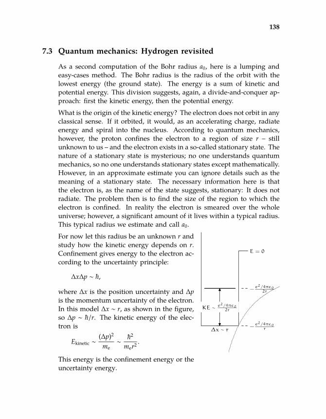
146 146

146 146

138

2010-05-13 00:43:32 / rev b667c9e4c1f1+

7.3 Quantum mechanics: Hydrogen revisited

As a second computation of the Bohr radius a0, here is a lumping andeasy-cases method. The Bohr radius is the radius of the orbit with thelowest energy (the ground state). The energy is a sum of kinetic andpotential energy. This division suggests, again, a divide-and-conquer ap-proach: first the kinetic energy, then the potential energy.

What is the origin of the kinetic energy? The electron does not orbit in anyclassical sense. If it orbited, it would, as an accelerating charge, radiateenergy and spiral into the nucleus. According to quantum mechanics,however, the proton confines the electron to a region of size r – stillunknown to us – and the electron exists in a so-called stationary state. Thenature of a stationary state is mysterious; no one understands quantummechanics, so no one understands stationary states except mathematically.However, in an approximate estimate you can ignore details such as themeaning of a stationary state. The necessary information here is thatthe electron is, as the name of the state suggests, stationary: It does notradiate. The problem then is to find the size of the region to which theelectron is confined. In reality the electron is smeared over the wholeuniverse; however, a significant amount of it lives within a typical radius.This typical radius we estimate and call a0.

E = 0

−e2/4πε02r

−e2/4πε0

r

KE ∼e2/4πε02r

∆x ∼ r

For now let this radius be an unknown r andstudy how the kinetic energy depends on r.Confinement gives energy to the electron ac-cording to the uncertainty principle:

∆x∆p ∼ ~,

where ∆x is the position uncertainty and ∆pis the momentum uncertainty of the electron.In this model ∆x ∼ r, as shown in the figure,so ∆p ∼ ~/r. The kinetic energy of the elec-tron is

Ekinetic ∼(∆p)2

me∼~2

mer2 .

This energy is the confinement energy or theuncertainty energy.

147 147

147 147

139

2010-05-13 00:43:32 / rev b667c9e4c1f1+

This estimate uses lumping twice. First, the complicated electrostaticpotential, which varies with distance, is replaced by the simple potentialwell (with infinitely high sides). Second, the electron, which in reality issmeared all over, is assumed to be at only one spot that is at a distance rfrom the proton.

This second lumping approximation also helps us estimate the potentialenergy. It is the classical electrostatic energy of a proton and electronseparated by r:

Epotential ∼ −e2

4πε0r.

Therefore, the total energy is the sum

E = Epotential + Ekinetic ∼ −e2

4πε0r+~2

mer2 .

With this total energy as its guide, the electron adjusts its separation r tomake the energy a minimum. As a step toward finding that separation,sketch the energy. For sketching functions, the first tool to try is easycases. Here, the easy cases are small and large r. At small r, kinetic energyis the important term because its 1/r2 overwhelms the 1/r in the potentialenergy. At large r, potential energy is the important term, because its 1/rgoes to zero more slowly than the 1/r2 in the kinetic energy.

E ∝

1/r2 (small r)−1/r (large r) (7.5)

E

r

Now we can sketch E in the two extremecases. The sketch demonstrates the re-sult in which we are interested: thatthere must be a minimum combined en-ergy at an intermediate value of r. Thereis no smooth way to connect the two ex-treme segments without introducing aminimum. An analytic argument con-firms that pictorial reasoning. At small r, the slope dE/dr is negative. Atlarge r, it is positive. At an intermediate r, the slope must cross betweenpositive and negative. In other words, somewhere in them middle theslope must be zero, and the energy must therefore be a minimum.

148 148

148 148

140

2010-05-13 00:43:32 / rev b667c9e4c1f1+

There are two approximate methods to determine the minimum r. Thefirst method is familiar from the analysis of lift in Section 3.5.2: When twoterms compete, the minimum occurs when the terms are roughly equal.In other words, at the minimum energy, the potential energy and kineticenergy (the two competing terms) are roughly equal in magnitude. Usingthe Bohr radius a0 as the corresponding separation, this criterion says

e2

4πε0a0︸ ︷︷ ︸PE

∼~2

mea20︸︷︷︸

KE

. (7.6)

The result for a0 is

a0 ∼~2

me(e2/4/4πε0). (7.7)

The second method of estimating the minimum-energy separation is touse dimensional analysis, by writing the energy and radius in dimension-less forms. Such a rewriting is not mandatory in this example, but it ishelpful in complicated examples and is therefore worth learning via thisexample. To make r dimensionless, cook up another length l and thendefine r ≡ r/l. The only other length that is based on the parameters ofhydrogen (and the relevant constants of nature such as ε0) is

l ≡ ~2

me(e2/4πε0).

So, let’s defined the scaled (dimensionless) radius as

r ≡ rl.

To make the energy dimensionless, cook up another energy based on theparameters of the problem. A reasonable candidate for this energy scaleis e2/4πε0l. That choice defines the scaled energy as

E ≡ Ee2/4πε0l

.

Using the scaled length and energy, the total energy

E = Epotential + Ekinetic ∼ −e2

4πε0r+~2

mer2

simplifies greatly:

149 149

149 149

141

2010-05-13 00:43:32 / rev b667c9e4c1f1+

E ∼ −1r

+1r2 .

The ugly constants all live in the definitions of scaled length and energy.This dimensionless energy is easy to think about and to sketch.

E

r

rmin

2

Calculus locates this minimum-energyr at rmin = 2. Equating the two termsr−1 and r−2 gives rmin ∼ 1. In normal,unscaled terms, it is

rmin = lrmin =~2

me(e2/4πε0),

which is the Bohr radius as computedusing dimensional analysis (Section 5.3.1) and is also the exact Bohr ra-dius computed properly using quantum mechanics. The sloppiness inestimating the kinetic and potential energies has canceled the error intro-duced by cheap minimization! Even if the method were not so charmed,there is no point in doing a proper calculus minimization. Given the inac-curacies in the rest of the derivation, The calculus method is too accurate

Engineers understand this idea of not over-engineering a system. If a bi-cycle most often breaks at welds in the frame, there is little point replacingthe metal between the welds with expensive, high-strength aerospace ma-terials. The new materials might last 100 years, but such a replacementwould be overengineering because something else will break before 100years are done.

In estimating the Bohr radius, the kinetic-energy estimate uses a crudeform of the uncertainty principle, ∆p∆x ∼ ~, whereas the true statementis that ∆p∆x ≥ ~/2. The estimate also uses the approximation Ekinetic ∼

(∆p)2/m. This approximation contains m instead of 2m in the denominator.It also assumes that ∆p can be converted into an energy as though itwere a true momentum rather than merely a crude estimate for the root-mean-square momentum. The potential- and kinetic-energy estimatesuse a crude definition of position uncertainty ∆x: that ∆x ∼ r. Aftermaking so many approximations, it is pointless to minimize the resultusing the elephant gun of differential calculus. The approximate methodis as accurate as, or perhaps more accurate than the approximations inthe energy.

150 150

150 150

142

2010-05-13 00:43:32 / rev b667c9e4c1f1+

The method of equating competing terms is called balancing. We bal-anced the kinetic energy against the potential energy by assuming thatthey are roughly the same size. Nature could have been unkind: Thepotential and kinetic energies could have differed by a factor of 10 or 100.But Nature is kind: The two energies are roughly equal, except for a con-stant that is nearly 1 (of order unity). This rough equality occurs in manyexamples: You often get a reasonable answer simply by pretending thattwo energies (or two quantities with the same units) are equal. [When thequantities are potential and kinetic energy, as they often are, you get extrasafety: The so-called virial theorem protects you against large errors (formore on the virial theorem, see any intermediate textbook on classicaldynamics).]

151 151

151 151

143

2010-05-13 00:43:32 / rev b667c9e4c1f1+

7.4 Boundary layers

Boundary layers, which are the final example of lumping, will help usexplain the drag paradox. That paradox arises in analyzing drag at highReynolds numbers (the usual case in everyday fluid motions). Dimen-sional analysis tells us that the drag coefficient cd is a function only of theReynolds number:

Fd12ρv2A

= f(rvν

), (7.8)

where Fd/ 12ρv2A is the drag coefficient, and rv/ν is the Reynolds number.

To make a high Reynolds number, take the limit in which the viscosityν approaches 0. Then viscosity vanishes from the analysis, as does theReynolds number. The result is that the drag coefficient is a function ofnothing – in other words, it is a constant. So far, so good: Empirically,at high Reynolds number, the drag coefficient is roughly constant andindependent of the Reynolds number.

The paradox arises upon looking at the Navier–Stokes equations:

(v·O)v +∂v∂t

= −1ρOp + νO2v. (7.9)

When the viscosity ν goes to zero, the νO2v viscous-stress term also van-ishes. However, the viscous-stress term is the only term that dissipatesenergy. (The pressure term Op is, like gravity, a conservative force fieldbecause it is the gradient of a scalar – the pressure – so it cannot dissi-pate energy.) Without the viscous-stress term, there can be no drag! So,at high Reynolds number, the drag coefficient should approach a constantbut that constant should be zero!. In real life, however, the drag is not zero;this discrepancy is the drag paradox.

Mathematically, the paradox is a failure of two operations to commute.The two operations are (1) solving the Navier–Stokes equations and (2)taking the viscosity to zero. If we first solve the Navier–Stokes equations,then we find that the drag coefficient is nonzero and roughly constant (i.e.independent of Reynolds number). If we then take the viscosity to zero(by taking the Reynolds number to infinity), no harm is done. Becausethe drag coefficient is roughly independent of Reynolds number, the dragcoefficient remains nonzero and roughly constant.

152 152

152 152

144

2010-05-13 00:43:32 / rev b667c9e4c1f1+

Now imagine applying the two operations in the reverse order. Takingthe viscosity to zero removes the viscous-stress term from the Navier–Stokes equations. Because that term is the only loss term, solving thesesimplified equations – called the Euler equations – produces a solutionwith zero drag. The mathematical formulation of the drag paradox is thatthe solution depends on the order in which one applies the operations ofsolving and taking a limit.This paradox, which remained a mystery for over 100 years, was resolvedby Prandtl in the early 1900s. The resolution identified the fundamentalproblem: that taking the viscosity to zero is a singular limit. That limitremoves the highest-order-derivative from the differential equation, so itchanges the equation from a second- to a first-order equation. This qual-itative change produces a qualitative change in behavior: from nonzerodrag to zero drag. To handle this change properly, Prandtl devised theconcept of a boundary layer – which we can understand using lumping.

ice

δ

vx = V

The explanation begins with the no-slip con-dition: In a fluid with viscosity (which meansall fluids), the fluid is at rest next to a solidobject. As an example, imagine wind blowingover a frozen lake. Just above the ice, and de-spite the wind, the air has zero velocity in thehorizontal direction. (In the vertical direction,the velocity is also zero because no air entersthe ice – that requirement is independent ofthe no-slip condition.) Far above the ice, the air has the speed of thewind. The boundary layer is the region above the ice over which the hor-izontal velocity vx changes from zero to the wind velocity. Actually, thehorizontal velocity never fully reaches the full wind velocity V (called thefree-stream velocity). But make the following lumping approximation:that vx increases linearly from 0 to V over a length δ – the thickness ofthe boundary layer.The boundary layer is a result of viscosity. The dimensions of viscosity,along with a bit of dimensional analysis, will help us estimate the thick-ness δ. The dimensions of ν are L2T−1. To make a thickness, multiply bya time and take the square root. But where does the time come from? Itis the time which the fluid has been flowing over the object. For example,for a golf ball moving at speed v, the time is roughly t ∼ r/v, where r isthe radius of the ball. Then

153 153

153 153

145

2010-05-13 00:43:32 / rev b667c9e4c1f1+

δ ∼√νt ∼

√νrv. (7.10)

Relative to the size of the object r, the dimensionless boundary-layer thick-ness δ/r is

δr∼

√νrv. (7.11)

The fraction inside the square root looks familiar: It is the reciprocal ofthe Reynolds number Re! Therefore

δr∼ Re−1/2. (7.12)

For most everyday flows, Re 1, so Re−1/2 1. The result is that the

boundary layer is a thin layer.

This thin layer will resolve the drag paradox. The intuition is that theboundary layer separates the flow into two regimes: inside and outsidethe boundary layer. Inside the boundary layer, viscosity has a large effecton the flow. Outside the boundary layer, the flow behaves as if viscositywere zero; there, the flow is described by the Euler equations (by theNavier–Stokes equations without the viscous-stress term). However, theboundary layer does not stick to the object everywhere. Generally, itdetaches somewhere on the back of the object. Once the boundary layerdetaches, a wake – the region behind the detached layer – is created,and the wake is turbulent. The wake has high-speed and therefore low-pressure flow: Bernoulli’s principle says that pressure p and velocity vare related by p + ρv2/2 = constant, so high v implies low p. Therefore,the front of the object experiences high pressure and the back experienceslow pressure. The result is drag. Intuitively, the drag coefficient is thefraction of the cross-sectional area covered by the turbulent wake.

ball

boundary layer

turbulent wake(low pressure)flow

154 154

154 154

146

2010-05-13 00:43:32 / rev b667c9e4c1f1+

That interpretation of the drag coefficient leads to an explanation of whythe drag coefficient remains roughly constant as the Reynolds numbergoes to infinity – in other words, as the flow speed increases or the vis-cosity decreases. In that limit, the boundary-layer detachment point shiftsas far forward as it goes, namely to the widest portion of the object. Thenthe drag coefficient is roughly 1.

This explanation mostly accounts for the high-Re data on drag coefficientversus Reynolds number. Here is the log–log plot from Section 5.6:

The drag coefficient is roughly constant in the Reynolds-number range 103

to (almost) 106. But why does the drag coefficient drop sharply aroundRe ∼ 106? The boundary-layer picture can also help us understand thisbehavior. To do so, first compute Reδ, the Reynolds number of the flowin the boundary layer. The Reynolds number is defined as

Re =typical flow speed × distance over which the flow speed varies

kinematic viscosity.

(7.13)

In the boundary layer, the flow speed varies from 0 to v, so it is comparableto v. The speed changes over the boundary-layer thickness δ. So

Reδ ∼vδν. (7.14)

Because δ ∼ r × Re−1/2,

155 155

155 155

147

2010-05-13 00:43:32 / rev b667c9e4c1f1+

Reδ ∼vrν× Re−1/2. (7.15)

The first fraction is just the regular Reynolds number Re, so

Reδ ∼ Re × Re−1/2 = Re1/2. (7.16)

ball

boundary layer

flow

Flows become turbulent when Re ∼ 103,so the boundary layer becomes turbu-lent when Reδ ∼ 103 or Re ∼ 106. Hmm!Somehow, the boundary layer’s becom-ing turbulent reduces the drag coefficient.Now recall the interpretation of the dragcoefficient as the fraction of the cross-sectional area covered by the turbu-lent wake. When the boundary layer becomes turbulent, it sticks to theobject much better, and detaches only near the back of the object. Theresult is less drag!

So, to get a low drag coefficient, make the object move fast enough thatthe Reynolds number is around 106. That high a Reynolds number is,however, difficult to achieve with a golf ball. That difficulty is the rea-son for the dimples on a golf ball. They trip the boundary layer intoturbulence at a lower Reynolds number. The golf ball then travels withthe benefit of this lower drag coefficient without needing to be hit at anunrealistically high speed.

156 156

156 156

148

2010-05-13 00:43:32 / rev b667c9e4c1f1+

Problem 7.5 PerfumeIf the diffusion constant (in air) for small perfume molecules is 10−6 m2 s−1,estimate the time for perfume molecules to diffuse across a room.

Now try the experiment: How long does it take to smell the perfume from acrossthe room? Explain the large discrepancy between the theoretical estimate andthe experimental value.

Problem 7.6 Bending of lightIn lecture we estimated how much gravity bends light by using dimensionalanalysis and then guessing the final functional form. In this problem, you ana-lyze the same situation using lumping.

As before, let r be the closest that the light gets to the origin (which is the centerof the gravitating mass). Discretize: Pretend that gravity forgets to deflect thephoton unless the photon’s distance to the origin is comparable to r. Using thatidea, estimate the radial (inward) velocity imparted to the photon, and then thebending angle.

Feel free to neglect dimensionless constants like 2 or π, and check your answeragainst what we derived in lecture.

Problem 7.7 Teacup spindownYou stir your afternoon tea to mix the milk (and sugar if you have a sweettooth). Once you remove the stirring spoon, the rotation starts to slow. What isthe spindown time τ? In other words, how long before the angular velocity ofthe tea has fallen by a significant fraction?

To estimate τ, consider a physicist’s idea of a teacup: a cylinder with height Land diameter L, filled with liquid. Why does the rotation slow? Tea near theedge of the teacup – and near the base, but for simplicity neglect the effect of thebase – is slowed by the presence of the edge (the no-slip boundary condition).The edge produces a velocity gradient.

Because of the tea’s viscosity, the velocity gradient produces a force on anypiece of the edge. This force tries to spin the piece in the direction of the tea’smotion. The piece exerts a force on the tea equal in magnitude and oppositein direction. Therefore, the edge slows the rotation. Now you can analyze thismodel quantitatively.

a. In terms of the total viscous force F and of the initial angular velocity ω,estimate the spindown time. Hint: Consider torque and angular momentum.(Feel free to drop any constants, such as π and 2, by invoking the EstimationTheorem: 1 = 2.)

b. You can estimate F with the idea that

viscous force ∼ ρν × velocity gradient × surface area.

157 157

157 157

149

2010-05-13 00:43:32 / rev b667c9e4c1f1+

Here ρν is η. The more familiar viscosity is η, known as the dynamic viscosity.The more convenient viscosity is ν, the kinematic viscosity. The velocitygradient is determined by the size of the region in which the the edge has asignificant effect on the flow; this region is called the boundary layer. Let δbe its thickness. Estimate the velocity gradient near the edge in terms of δ,and use the equation for viscous force to estimate F.

c. Put your expression for F into your earlier estimate for τ, which should nowcontain only one quantity that you have not yet estimated (the boundary-layerthickness).

d. You can estimate δ using your knowledge of random walks. The boundarylayer is a result of momentum diffusion; just as D is the molecular-diffusioncoefficient, ν is the momentum-diffusion coefficient. In a time t, how far canmomentum diffuse? This distance is δ. What is a natural estimate for t?(Hint: After rotating 1 radian, the fluid is moving in a significantly differentdirection than before, so the momentum fluxes no longer add.) Use that timeto estimate δ.

e. Now put it all together: What is the characteristic spindown time τ (the timefor the rotation to slow down by a significant amount)?

f. Stir some tea to experimentally estimate τexp. Compare this time with thetime predicted by the preceding theory. [In water (and tea is roughly water),ν ∼ 210−6 m2 s−1.]

Problem 7.8 Stokes’ lawYou can use ideas from Problem 7.7 to derive Stokes’ formula for drag at lowspeeds (more precisely, at low Reynolds’ number). In the text we derived theresult from dimensional analysis; here you will develop a physical argument.

Consider a sphere of radius R moving with velocity v. Equivalently, in thereference frame of the sphere, the sphere is fixed and the fluid moves past itwith velocity v. Next to the sphere, the fluid is stationary. Over a region ofthickness δ (the boundary layer), the fluid velocity rises from zero to the fullflow speed v. Assume that δ ∼ R (the most natural assumption) and estimatethe viscous drag force. Compare the force with Stokes’ formula (remember thatρν = η).

Problem 7.9 Bouncing ballYou drop a steel ball, say r ∼ 1 cm, from a height of one or two metres. It landson a steel surface and bounces up to nearly the original drop height. Estimatethe contact force at the instant when the ball is stationary on the ground. Giveyour answer as the dimensionless ratio

contact forceweight of the ball

.

Useful data: The elastic modulus of steel is Y ∼ 1011 Nm−2.

158 158

158 158

150

2010-05-13 00:43:32 / rev b667c9e4c1f1+

Problem 7.10 Cone free-fall time and distanceEstimate how long the falling cones of Section 3.3.1 require to reach (a goodfraction of) terminal velocity. And estimate how far they fall before reaching (agood fraction of) terminal velocity.

Problem 7.11 Kinetic theoryMolecules in a gas travel in all directions and with a continuous range of speeds.However, many results can be understood with the following lumping approxi-mation: Pretend that all molecules move with the thermal speed and that theymove only along a coordinate axis (i.e. in one of six directions).

Using the preceding lumping approximation, compute the following quantities:

Problem 7.12 Electric field of a uniform sheet of charge

Problem 7.13 Electric field inside a uniform shell of charge

159 159

159 1592010-05-13 00:43:32 / rev b667c9e4c1f1+

8Probabilistic reasoning

8.1 Is it my telephone number? 1518.2 Why divide and conquer works 1558.3 Random walks 168

The set of tools under discussion in this part – which so far have in-cluded easy cases and lumping – all offer ways to handle complexity bydiscarding information. The next tool in this set is probabilistic reason-ing. Instead of trying to force the world to give us exact and completeinformation, we accept that our information will be incomplete and useprobability to quantify the incompleteness.

8.1 Is it my telephone number?

To introduce the fundamental ideas, here is an example from soon afterI had moved to England sometime in the last century. I was talking to afriend on the phone, and he needed to call me back. Having just movedto the apartment, I was still unsure of my phone number (plus, Britishphone numbers have a strange format). I had a guess, which I thoughtwas reasonably likely, but I was not very sure of it. To test it, I picked upmy phone, dialed the candidate number, and got a busy signal.

Given this experimental evidence, how sure am I that the candidate number ismy phone number? To make the question quantitative: What odds should I give?

This question makes no sense if one uses the view of probability as long-run frequency. In that view – alas, the most common view – the proba-bility of, say, a coin turning up heads is 1/2 because 1/2 is the limiting

160 160

160 160

152

2010-05-13 00:43:32 / rev b667c9e4c1f1+

proportion of heads in an ever-longer series of tosses. However, for eva-lutin the plausibility of the phone number, this interpretation – calledthe frequentist interpretation – makes no sense. What is the repeatedexperiment analogous to tossing the coin repeatedly? There is none.

The frequentist interpretation places probability in the physical systemitself, as an objective property of the system. For example, the probabilityof 1/2 for tossing heads is seen as a property of the coin itself. Thatplacement is incorrect and is the reason that the frequentist interpretationcannot answer the phone-number question. The sensible alternative – thatprobability reflects the incompleteness of our knowledge – is known asthe Bayesian interpretation of probability.

The Bayesian interpretation is based on a two simple ideas. First, proba-bilities reflect our state of certainty about a hypothesis. Probabilities areexplicitly subjective: Someone with a different set of knowledge will usea different set of probabilities. Second, by collecting evidence, our stateof certainty changes. In other words, evidence changes our probabilityassignments.

In the phone-number problem, the hypothesis H is that my candidatenumber is correct. For this hypothesis, I have an initial or prior probabilityP(H). After collecting the evidence E – that when I dialed this numberthe phone was busy – I make a new probability assignment P(H|E) (theprobability of the hypothesis H given the evidence E).

The recipe for using evidence to update probabilities is known as Bayestheorem. To derive it, imagine that the mental world contains only twohypothesis H and H, with probabilities P(H) and P(H) = 1 − P(H), andthat we have collected some evidence E. Now write the joint probabilityP(H&E) in two different ways. P(H&E) is the probability of H beingtrue and E occurring. That probability is, first, the product P(H|E)P(E)– namely, the probability that H is true given that E occurs times theprobability that E occurs. P(H&E) is, second, the product P(E|H)P(H)– namely, the probability that E occurs given that H is true times theprobability that H is true. These two paths to H&E must produce identicalprobabilities, so

P(E|H)P(H) = P(H|E)P(E). (8.1)

Our goal is the updated probability of the hypothesis, namely P(H|E). Itis given by

161 161

161 161

153

2010-05-13 00:43:32 / rev b667c9e4c1f1+

P(H|E) =P(E|H)P(H)

P(E). (8.2)

Similarly, for the opposite hypothesis H,

P(H|E) =P(E|H)P(H)

P(E). (8.3)

Using the ratio P(H|E)/P(H|E), which is known as the odds, gives aneven simpler formula because P(E) is common to both probabilities andtherefore cancels out:

P(H|E)P(H|E)

=P(E|H)P(H)P(E|H)P(H)

. (8.4)

The right side contains the factor P(H)/P(H), which is the initial odds.Using O for odds,

O(H|E) = O(H) ×P(E|H)P(E|H)

. (8.5)

This result is Bayes theorem (for the case of two mutually exclusive hy-potheses).

In the fraction P(E|H)/P(E|H), the numerator measures how well the hy-pothesis H explains the evidence E; the denominator measures how wellthe contrary hypothesis H explains the same evidence. Their ratio, knownas the likelihood ratio, measures the relative value of the two hypothesisin explaining the evidence. So, Bayes theorem has the following Englishtranslation:

updated odds = initial odds × relative explanatory power. (8.6)

Let’s see how this result applies to my English telephone number. InitiallyI was not very sure of the phone number, so P(H) is perhaps 1/2 and O(H)is 1. In the likelihood ratio, the numerator P(E|H) is the probability ofgetting a busy signal given that my guess is correct (given that H is true).If my guess is correct, I’d be dialing my own phone using my phone, soI would definitely get a busy signal: P(E|H) = 1. The hypothesis of acorrect number is a very good explanation of the data.

The trickier estimate is P(E|H): the probability of getting a busy signalgiven that my guess is incorrect (given that H is true). If my guess is

162 162

162 162

154

2010-05-13 00:43:32 / rev b667c9e4c1f1+

incorrect, I’d be dialing a random person’s phone. What is the probabilitythat a random phone is busy? I figure it’s similar to the fraction of theday that my phone is busy. In my household, the adults use the phonemaybe 1 hour per day (and the children are not yet able to use a phone).So the busy fraction is perhaps the ratio of 1 hour to 24 hours, or 1/24.But that’s an underestimate. At 3am I would not do the experiment –in case I am wrong and wake someone up. Equally, I am not often onthe phone at 3am. A more reasonable denominator is probably 10 or 12hours, making the busy fraction roughly 0.1. In other words, P(E|H) ∼ 0.1.The hypothesis of an incorrect number is not a very good explanation forthe data. The relative explanatory power, which is the likelihood ratio, is

P(E|H)P(E|H)

∼1

0.1= 10. (8.7)

Therefore, the updated odds are

O(H|E) = O(H) ×P(E|H)P(E|H)

= 10, (8.8)

or 10-to-1 odds in favor of the number (at the start the odds were 1 to 1).The guess become very plausible!

163 163

163 163

155

2010-05-13 00:43:32 / rev b667c9e4c1f1+

8.2 Why divide and conquer works

How does divide-and-conquer reasoning (Chapter 1) produce such ac-curate estimates? Alas, this problem is hard to analyze directly becausewe do not know the accuracy in advance. But we can analyze a relatedproblem: how divide-and-conquer reasoning increases our confidence inan estimate or, more precisely, decreases our uncertainty.The telegraphic answer is that it works by subdividing a quantity aboutwhich we know little into several quantities about which we know more.Even if we need many subdivisions before we reach reliable information,the increased certainty outweighs the small penalty for combining manyquantities. To explain that telegraphic answer, let’s analyze in slowmotiona short estimation problem using divide-and-conquer done.

8.2.1 Area of a sheet of paper

The slow-motion problem is to estimate area of a sheet of A4 paper (A4is the standard sheet size in Europe). On first thought, even looking at asheet I have little idea about its area. On second thought, I know some-thing. For example, the area is more than 1 cm2 and less than 105 cm2.That wide range makes it hard to be wrong but is also too wide to beuseful. To narrow the range, I’ll drew a small square with an area ofroughly 1 cm2 and guess how many squares fit on the sheet: probably atleast a few hundred and at most a few thousand. Turning ‘few’ into 3, Ioffer 300 cm2 to 3000 cm2 as a plausible range for the area.Now let’s use divide-and-conquer and get a more studied range. Subdi-vide the area into the width and height; about two quantities my knowl-edge is more precise than it is about area itself. The extra precision has ageneral reason and a reason specific to this problem. The general reason isthat we have more experience with lengths than areas: Which is the morefamiliar quantity, your height or your cross-sectional area? Therefore, ourlength estimates are usually more accurate than our area estimates.The reason specific to this problem is that A4 paper is the Europeanequivalent of standard American paper. American paper is known tocomputers and laser printers as ‘letter’ paper and known commonly inthe United States as ‘eight-and-a-half by eleven’ (inches!). In metric units,those dimensions are 21.59 cm × 27.94 cm. If A4 paper were identical toletter paper, I could now compute its exact area. However, A4 paper is, I

164 164

164 164

156

2010-05-13 00:43:32 / rev b667c9e4c1f1+

remember from living in England, slightly thinner and longer than letterpaper. I forget the exact differences between the dimensions of A4 andletter paper, hence the remaining uncertainty: I’ll guess that the widthlies in the range 19 . . . 21 cm and the length lies in the range 28 . . . 32 cm.

The next problem is to combine the plausible ranges for the height andwidth into the plausible range for the area. A first guess, because thearea is the product of the width and height, is to multiply the endpointsof the width and height ranges:

Amin = 19 cm × 28 cm = 532 cm2;Amax = 21 cm × 32 cm = 672 cm2.

This method turns out to overestimate the range – a mistake that I correctlater – but even the too-large range spans only a factor of 1.26 whereas thestarting range of 300 . . . 3000 cm2 spans a factor of 10. Divide and conquerhas significantly narrowed the range by replacing quantities about whichwe have little knowledge, such as the area, with quantities about whichwe have more knowledge.

The second bonus, which I now quantify correctly, is that subdividinginto many quantities carries only a small penalty, smaller than suggestedby naively multiplying endpoints. The naive method overestimates therange because it assumes the worst. To see how, imagine an extremecase: estimating a quantity that is the product of ten factors, each thatyou know to within a factor of 2 (in other words, each plausible rangeis a factor of 4). Is your plausible range for the final quantity a factor of410≈ 106?! That conclusion is terribly pessimistic. A more likely result

is that a few of the ten estimates will be too large and a few too small,allow several errors to cancel.

To quantify and fix this pessimism, I will explain plausible ranges usingprobabilities. Probabilities are the tool for this purpose. As discussedin Section 8.1, probabilities reflect incomplete knowledge; they are notfrequencies in a random experiment (Jaynes’s Probability Theory: The Logicof Science [11] is a excellent, book-length discussion and application of thisfundamental point).

To make a probabilistic description, start with the proposition or hypoth-esis

H ≡ The area of A4 lies in the range 300 . . . 3000 cm2.

165 165

165 165

157

2010-05-13 00:43:32 / rev b667c9e4c1f1+

and information (or evidence)

I ≡What I know about the area before using divide and conquer.

Now I want to find the conditional probability P(H|I) – namely, the prob-ability of H given my knowledge before trying divide and conquer. Thereis no known algorithm for computing a probability in such a complicatedproblem situation. How, for example, does one represent my state ofknowledge? In these cases, the best we can do is to introspect or, in plainEnglish, to talk to our gut.

My gut is the organ with the most access to my intuitive knowledge andits incompleteness, and it tells me that I would feel mild surprise but notshock if I learned that the true area lay outside the range 300 . . . 3000 cm2.The surprise suggests that P(H|I) is larger than 1/2. The mildness of thesurprise suggests that P(H|I) is not much larger than 1/2. I’ll quantify itas P(H|I) = 2/3: I would give 2-to-1 odds that the true area is within theplausible range.

Furthermore, I’ll use this probability or odds to define a plausible range:It is the range for which I think 2-to-1 odds is fair. I could have used a1-to-1 odds range instead, but the 2-to-1 odds range will later help giveplausible ranges an intuitive interpretation (as a region on a log-normaldistribution). That interpretation will then help quantify how to combineplausible ranges.

For the moment, I need only the idea that the plausible range containsroughly 2/3 of the probability. With a further assumption of symmetry,the plausible range 300 . . . 3000 cm2 represents the following probabilities:

P(A < 300 cm2) = 1/6;P(300 cm ≤ A ≤ 3000 cm2) = 2/3;

P(A > 3000 cm2) = 1/6.

Here is the corresponding picture with width proportional to probability:

< 300 cm2 300 . . . 3000 cm2 > 3000 cm2

p ≈ 1/6 p ≈ 2/3 p ≈ 1/6

A

For the height h and width w, after doing divide and conquer and us-ing the similarity between A4 and letter paper, the plausible ranges are

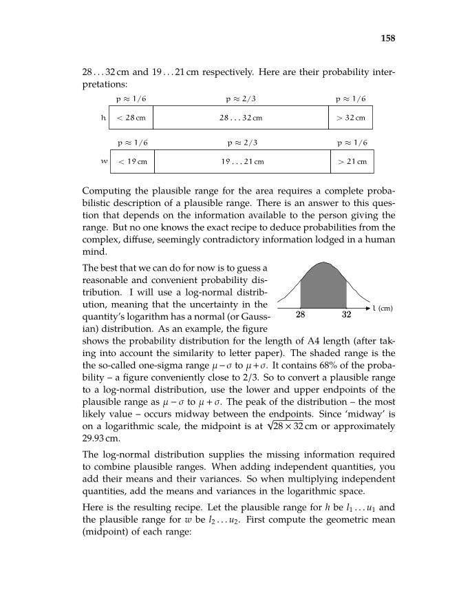
166 166

166 166

158

2010-05-13 00:43:32 / rev b667c9e4c1f1+

28 . . . 32 cm and 19 . . . 21 cm respectively. Here are their probability inter-pretations:

< 28 cm 28 . . . 32 cm > 32 cm

p ≈ 1/6 p ≈ 2/3 p ≈ 1/6

h

< 19 cm 19 . . . 21 cm > 21 cm

p ≈ 1/6 p ≈ 2/3 p ≈ 1/6

w

Computing the plausible range for the area requires a complete proba-bilistic description of a plausible range. There is an answer to this ques-tion that depends on the information available to the person giving therange. But no one knows the exact recipe to deduce probabilities from thecomplex, diffuse, seemingly contradictory information lodged in a humanmind.

2828 3232l (cm)

The best that we can do for now is to guess areasonable and convenient probability dis-tribution. I will use a log-normal distrib-ution, meaning that the uncertainty in thequantity’s logarithm has a normal (or Gauss-ian) distribution. As an example, the figureshows the probability distribution for the length of A4 length (after tak-ing into account the similarity to letter paper). The shaded range is thethe so-called one-sigma range µ−σ to µ+σ. It contains 68% of the proba-bility – a figure conveniently close to 2/3. So to convert a plausible rangeto a log-normal distribution, use the lower and upper endpoints of theplausible range as µ− σ to µ+ σ. The peak of the distribution – the mostlikely value – occurs midway between the endpoints. Since ‘midway’ ison a logarithmic scale, the midpoint is at

√28 × 32 cm or approximately

29.93 cm.The log-normal distribution supplies the missing information requiredto combine plausible ranges. When adding independent quantities, youadd their means and their variances. So when multiplying independentquantities, add the means and variances in the logarithmic space.Here is the resulting recipe. Let the plausible range for h be l1 . . . u1 andthe plausible range for w be l2 . . . u2. First compute the geometric mean(midpoint) of each range:

167 167

167 167

159

2010-05-13 00:43:32 / rev b667c9e4c1f1+

µ1 =√

l1u1;

µ2 =√

l2u2.

The midpoint of the range for A = hw is the product of the two midpoints:

µ = µ1µ2. (8.9)

To compute the plausible range, first compute the ratios measuring thewidth of the ranges:

r1 = u1/l1;r2 = u2/l2.

These ratios measure the width of the ranges. The combined ratio – thatis, the ratio of endpoints for the combined plausible range – is

r = exp(√

(ln r1)2 + (ln r2)2).

For approximate range calculations, the following contour graphs oftenprovide enough accuracy:

11

2

2

2

5

5

5 10

10

10

r1

r2

11

1.5

1.5

1.52

2

2

r1

r2

After finding the range, choose the lower and upper endpoints l and u tomake u/l = r and

√lu = µ. In other words, the plausible range is

µ√

r. . . µ√

r.

Problem 8.1 Deriving the ratioUse Bayes theorem to confirm this method for combining plausible ranges.

Let’s check this method in a simple example where the width and heightranges are 1 . . . 2m. What is the plausible range for the area? The naive

168 168

168 168

160

2010-05-13 00:43:32 / rev b667c9e4c1f1+

approach of simply multiplying endpoints produces a plausible range of1 . . . 4m2 – a width of a factor of 4. However, this range is too pessimisticand the correct range should be narrower. Using the log-normal distrib-ution, the range spans a factor of

exp(√

2 × (ln 2)2)≈ 2.67.

This span and the midpoint determine the range. The area midpoint isthe product of the width and height midpoints, each of which is

√2m.

So the midpoint is 2m2. The correct endpoints of the plausible range aretherefore

2m2√

2.67. . . 2m2

×

√

2.67

or 1.23 . . . 3.27m2. In other words, I assign roughly a 1/6 probabilitythat the area is less than 1.23m2 and roughly a 1/6 probability that itis greater than 3.27m2. Those conclusions seem reasonable when usingsuch uncertain knowledge of length and width.

Having checked that the method is reasonable, it is time to test it in theoriginal illustrative problem: the plausible area range for an A4 sheet. Thenaive plausible range was 532 . . . 672 cm2, and the correct plausible rangewill be narrower. Indeed, the log-normal method gives the narrower arearange of 550 . . . 650 cm2 with a best guess (most likely value) of 598 cm2.How did we do? The true area is exactly 2−4 m2 or 625 cm2 because – Iremembered only after doing this calculation! – An paper is constructedto have one-half the area of A(n−1) paper, with A0 paper having an areaof 1m2. The true area is only 5% larger than the best guess, suggestingthat we used accurate information about the length and width; and it fallswithin the plausible range but not right at the center, suggesting that themethod for computing the plausible range is neither too daring nor tooconservative.

The analysis of combining ranges illustrates the two crucial points aboutdivide-and-conquer reasoning. First, the main benefit comes from subdi-viding vague knowledge (such as the area itself) into pieces about whichour knowledge is accurate (the length and the width). Second, this ben-efit swamps the small penalty in accuracy that results from combiningmany quantities together.

169 169

169 169

161

2010-05-13 00:43:32 / rev b667c9e4c1f1+

8.2.2 Gold or bills?

The next estimation example is dedicated to readers who forgot careers inthe financial industry for less lucrative careers in teaching and research.

Having broken into a bank vault, should we take the bills or the gold?

The answer depends partly on the ease and costs of fencing the loot– an analysis beyond the scope of this book. Within our scope is thefollowing question: Which choice lets us carry out the most money? Ourcarrying capacity is limited by weight and volume. For this analysis, let’sassume that the more stringent limit comes from weight or mass. Thenthe decision divides into two subproblems: the value per mass for USbills and the value per mass for gold. In order to decide which to take,we’ll compute both values per mass and their respective plausible ranges.

gold or bills?

value/mass for $100 bill

value$100

mbill

???

value/mass for gold

value of 1 oz of gold???

m

1 oz

Two leaves have defined values: the value of a bill and the mass of 1 oz (1ounce) of gold. The two other leaves need divide-and-conquer estimates.In the first round of analysis, make point estimates; then, in the secondround, account for the uncertainty by using the plausible-range methodof Section 8.2.

The value of gold is, I vaguely remember, around $800/oz. As a roughcheck on the value – for example, should it be $80/oz or $8000/oz? –here is a historical method. In 1945, at the end of World War 2, theBritish empire had exhausted its resources while the United States be-came the world’s leading economic power. The gold standard, which fellapart during the depression, was accordingly reinstituted in terms of thedollar: $35 would be the value of 1 oz of gold. Since then, inflation hasprobably devalued the dollar by a factor of 10 or more, so gold should beworth around $350/oz. My vague memory of $800/oz therefore seemsreasonable.

170 170

170 170

162

2010-05-13 00:43:32 / rev b667c9e4c1f1+

mass

ρ V

w h t

For the bill, its mass breaks into density (ρ) times vol-ume (V), and volume breaks into width (w) times height(h) times thickness (t). To estimate the height and width,I could lay down a ruler or just find any bill – all US billsare the same size – and eyeball its dimensions. A $1 billseems to be few inches high and 6 in wide. In metricunits, those dimensions are h ∼ 6 cm and w ∼ 15 cm. [Toimprove your judgment for sizes, first make guesses; then, if you feel un-sure, check the guess using a ruler to check. With practice, your need forthe ruler will decrease and your confidence and accuracy will increase.]

The thickness, alas, is not easy to estimate by eye or with a ruler. Isthe thickness 1mm or 0.1mm or 0.01mm? Having experience with suchsmall lengths, my eye does not not help much. My ruler is calibratedin steps of 1mm, from which I see that a piece of paper is significantlysmaller than 1mm, but I cannot easily see how much smaller.

An accurate divide-and-conquer estimate, we learned in Section 8.2, de-pends on replacing a vaguely understood quantity with accurately knownquantities. Therefore to estimate the thickness accurately, I connect it tofamiliar quantities. Bills are made from paper, a ubiquitous substance(despite hype about the paperless office). Indeed, a ream of printer paperis just around the corner. The thickness of the ream and the number ofsheets that it contains determines the thickness of one sheet:

t =treamNream

.

You might call this approach ‘multiply and conquer’. The general les-son for accurate estimation is to magnify values much smaller than ourexperience, and and to shrink values much bigger than our experience.

m

ρ V

h w t

tream Nream

The magnification argument adds one levelto the tree and replaces one leaf with twoleaves on the new level. Two of the fiveleaf nodes are already estimated. A reamcontains 500 sheets (Nream = 500) and hasa thickness of roughly 2 in or 5 cm.

What is the estimate for ρ, the density of abill?

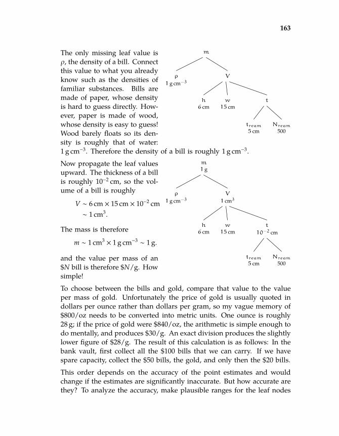
171 171

171 171

163

2010-05-13 00:43:32 / rev b667c9e4c1f1+

m

ρ

1 g cm−3

V

h

6 cmw

15 cmt

tream5 cm

Nream500

The only missing leaf value isρ, the density of a bill. Connectthis value to what you alreadyknow such as the densities offamiliar substances. Bills aremade of paper, whose densityis hard to guess directly. How-ever, paper is made of wood,whose density is easy to guess!Wood barely floats so its den-sity is roughly that of water:1g cm−3. Therefore the density of a bill is roughly 1g cm−3.

m

1 g

ρ

1 g cm−3

V

1 cm3

h

6 cmw

15 cmt

10−2 cm

tream5 cm

Nream500

Now propagate the leaf valuesupward. The thickness of a billis roughly 10−2 cm, so the vol-ume of a bill is roughly

V ∼ 6 cm × 15 cm × 10−2 cm∼ 1 cm3.

The mass is therefore

m ∼ 1 cm3× 1g cm−3

∼ 1g.

and the value per mass of an$N bill is therefore $N/g. Howsimple!

To choose between the bills and gold, compare that value to the valueper mass of gold. Unfortunately the price of gold is usually quoted indollars per ounce rather than dollars per gram, so my vague memory of$800/oz needs to be converted into metric units. One ounce is roughly28g; if the price of gold were $840/oz, the arithmetic is simple enough todo mentally, and produces $30/g. An exact division produces the slightlylower figure of $28/g. The result of this calculation is as follows: In thebank vault, first collect all the $100 bills that we can carry. If we havespare capacity, collect the $50 bills, the gold, and only then the $20 bills.

This order depends on the accuracy of the point estimates and wouldchange if the estimates are significantly inaccurate. But how accurate arethey? To analyze the accuracy, make plausible ranges for the leaf nodes

172 172

172 172

164

2010-05-13 00:43:32 / rev b667c9e4c1f1+

and propagate them upward – thereby obtaining plausible ranges for thevalue per mass of bills and gold.

Problem 8.2 Your plausible rangesWhat are your plausible ranges for the five leaf quantities tream, Nream, w, h,and ρ? Propagate them upward to get plausible ranges for the interior nodesincluding for the root node m.

Here are my ranges along with a few notes on how I estimated a few ofthem:

1. thickness of a ream, tream: 4 . . . 6 cm.

2. number of sheets in a ream, Nream: 500. I’m almost certain that I re-member this value correctly, but to be certain I confirmed it by lookingat a label on a fresh ream.

3. width of a bill, w: 10 . . . 20 cm. A reasonable length estimate seemedto be 6 in but I could give or take a couple inches. In metric units,4 . . . 8 in becomes (roughly) 10 . . . 20 cm.

4. height of a bill, h: 5 . . . 7 cm.

5. density of a bill, ρ: 0.8 . . . 1.2g cm−3. The argument for ρ = 1g cm−3 –that a bill is made from paper and paper is made from wood – seemsreasonable. However, the many steps required to process wood intopaper may reduce or increase the density slightly.

Now propagate these ranges upward. The plausible range for the thick-ness t becomes 0.8 . . . 1.2 ·10−2 cm. The plausible range for the volume Vbecomes 0.53 . . . 1.27 cm3. The plausible range for the mass m becomes0.50 . . . 1.30g. The plausible range for the value per mass is $79. . . 189/g(with a midpoint of $122/g).

gold or bills?

value/mass for $100 bill

value$100

mbill

0.50 . . . 1.30 g

value/mass for gold

value of 1 oz of gold$400. . . 900

m

27. . . 30 g

The next estimateis the value permass of gold. Ican be as accu-rate as I want inconverting fromounces to grams.But I’ll be lazyand try to remember the value while including uncertainty to reflect the

173 173

173 173

165

2010-05-13 00:43:32 / rev b667c9e4c1f1+

fallibility of memory; let’s say that 1oz = 27 . . . 30g. This range spansonly a factor of 1.1, but the value of an ounce of gold will have a widerplausible range (except for those who often deal with financial markets).My range is $400. . . 900. The mass and value ranges combine to give$14. . . 32/g as the range for gold.

Here is a picture comparing the range for gold with the ranges for UScurrency denominations:

$100 bill7979 189189

$50 bill4040 9595

$20 bill1616 3838

$10 bill88 1919

gold1414 3232

$/g (log scale)

Looking at the locations of these ranges and overlaps among them, I amconfident that the $100 bills are worth more (per mass) than gold. I amreasonably confident that $50 bills are worth more than gold, undecidedabout $20 bills, and reasonably confident that $10 bills are worth less thangold.

174 174

174 174

166

2010-05-13 00:43:32 / rev b667c9e4c1f1+

8.2.3 Oil imports using plausible ranges

To confirm these lessons, examine the benefit of divide-and-conquer rea-soning in the example from Section 1.4: estimating the annual US oilimports. To quantify the benefit, I compare my plausible ranges beforeand after using divide and conquer.

Before I use divide and conquer, I have almost no idea what the oil im-ports are, and I am scared even to guess. To nudge me along, I imagine amugger demanding, ‘Your guess or your life!’ In which case I counterofferwith, ‘Can I give you a range instead of a number? I’d be surprised if theannual imports are less than107 barrels/yr or more than 1012 barrels/yr.’The imaginary mugger, being my own creation, always accepts my offer.

Problem 8.3 Your rangeWhat is your plausible range for the annual oil imports?

I need little prodding to narrow my plausible range using divide-and-conquer reasoning. It required making several estimates:

1. Npeople: US population;

2. fcar: cars per person;

3. l: average distance that a car is driven

4. m: average gas mileage;

5. V: volume of a barrel;

6. fother: factor to multiply auto consumption to include all other con-sumption;

7. fimported: fraction of oil that is imported.

Problem 8.4 Your rangesGive your plausible range for each quantity, i.e. the range for which you assigna two-thirds probability that the true value lies within the range.

Here are my plausible ranges with a few notes of explanation:

1. Npeople: 290–310 million. I recently read in the newspaper that theUS population just reached the milestone of 300 million. How muchshould I believe what I read in the paper? The media lie when itserves the powerful, but I cannot find any reason to lie about the US

175 175

175 175

167

2010-05-13 00:43:32 / rev b667c9e4c1f1+

population, so I trust the figure, and throw in a bit of uncertaintyto reflect the difficulties encountered in counting the population (e.g.what about undocumented immigrants, who are unlikely to fill outcensus forms?).

2. fcar: 0.5–1.5.

3. l: 7 · 103–20 · 103 mi. Some books assessing used cars consider a low-mileage car to have less than 104 mi per year of age. So I guess that theaverage is somewhat larger than 104 mi/yr. But I am not confident ofmy recollection or the deduction, so my plausible range spans a factorof 3.

4. m: 15–40miles/gallon;

5. V: 30–60gallons;

6. fother: 1.5–3;

7. fimported: 0.3–0.8.

What is the resulting plausible range for the oil imports?

Now combine the ranges using the method we used for the area of asheet of A4 paper. That method produces the following plausible range:

1.0 . . . 3.1 . . . 9.6 ·109 barrels/year.

Compare this range to the range for the off-the-cuff guess 107 . . . 1012 barrels/yr.That range spanned a factor of 105 whereas the improved range spans amere factor of 10 – thanks to divide-and-conquer reasoning.

176 176

176 176

168

2010-05-13 00:43:32 / rev b667c9e4c1f1+

8.3 Random walks

Random walks are everywhere. Do you remember the card game War?How long does it last, on average? A molecule of neurotransmitter isreleased from a vesicle. Eventually it binds to the synapse; then your legtwitches. How long does the molecule take to arrive? On a winter day,you stand outside wearing only a thin layer of clothing. Why do you feelcold?

These physical situations are examplesof random walks – for example, a gasmolecule moving and colliding. The analy-sis in this section is in three parts. First,we figure out how random walks be-have. Then we use that knowledge toderive the diffusion equation, which isa reusable idea (an abstraction). Finally,we apply the diffusion equation to heat flows (keeping warm on a coldday).

8.3.1 Behavior of regular walks

In a general random walk, the walker can move a variable distance andin any direction. This general situation is complicated. Fortunately, theessential features of the random walk do not depend on these compli-cated details. Let’s simplify. The complexity arises from the generality– namely, because the direction and the distance between collisions arecontinuous. To simplify, lump the possible distances: Assume that theparticle can travel only a fixed distance between collisions. In addition,lump the possible directions: Assume that the particle can travel onlyalong coordinate axes. Further specialize by analyzing the special case ofone-dimensional motion before going to the more general cases of two-and three-dimensional motion.

In this lumped one-dimensional model, a particle starts at the origin andmoves along a line. At each tick it moves left or right with probability1/2 in each direction. Here it is at x = 3:

−5 −4 −3 −2 −1 0 1 2 3 4 5 6x

177 177

177 177

169

2010-05-13 00:43:32 / rev b667c9e4c1f1+

Let the position after n steps be xn, and the expected position after n stepsbe 〈xn〉. The expected is position is the average of all its possible positions,weighted by their probabilities. Because the random walk is unbiased –motion in each direction is equally likely – the expected position cannotchange (that’s a symmetry argument).

〈xn〉 = 〈xn−1〉 .

Therefore, 〈x〉, the first moment of the position, is an invariant. Alas, itis not a fascinating invariant because it does not tell us anything that wedid not already understand.

Let’s try the next-most-complicated moment: the second moment 〈x2〉.

Its analysis is easiest in special cases. Suppose that, after wandering awhile, the particle has arrived at 7, i.e. x = 7. At the next tick it will beat either x = 6 or x = 8. Its expected squared position – not its squaredexpected position! – has become

〈x2〉 =

12(62 + 82

)= 50.

The expected squared position increased by 1.

Let’s check this pattern with a second example. Suppose that the particleis at x = 10, so 〈x2

〉 = 100. After one tick, the new expected squaredposition is

〈x2〉 =

12(92 + 112

)= 101.

Yet again 〈x2〉 has increased by 1! Based on those two examples, the

conclusion is that

〈x2n+1〉 = 〈x2

n〉 + 1.

In other words,

〈x2n〉 = n.

Because each step takes the same time (the particle moves at constantspeed),

〈x2n〉 ∝ t.

178 178

178 178

170

2010-05-13 00:43:32 / rev b667c9e4c1f1+

The result that 〈x2〉 is proportional to time applies not only to the one-

dimensional random walk. Here’s an example in two dimensions. Sup-pose that the particle’s position is (5, 2), so 〈x2

〉 = 29. After one step, ithas four equally likely positions:

(0,0)(0,0)

(5,2)

r

Rather than compute the new expected squared distance using all fourpositions, be lazy and just look at the two horizontal motions. The twopossibilities are (6, 2) and (4, 2). The expected squared distance is

〈x2〉 =

12

(40 + 20) = 30,

which is one more than the previous value of 〈x2〉. Since nothing is special

about horizontal motion compared to vertical motion – symmetry! – thesame result holds for vertical motion. So, averaging over the four possiblelocations produces an expected squared distance of 30.For two dimensions, the pattern is:

〈x2n+1〉 = 〈x2

n〉 + 1.

No step in the analysis depended on being in only two dimensions. Infancy words, the derivation and the result are invariant to change of di-mensionality. In plain English, this result also works in three dimensions.In a standard walk in a straight line, 〈x〉 ∝ time. Note the single powerof x. The interesting quantity in a regular walk is not x itself, since itcan grow without limit and is not invariant, but the ratio x/t, which isinvariant to changes in t. This invariant is known as the speed.In a random walk, where 〈x2

〉 ∝ t, the interesting quantity is 〈x2〉/t. The

expected squared position is not invariant to changes in t. However,the ratio 〈x2

〉/t is invariant. This invariant is, except for a dimensionlessconstant, the diffusion constant and is often denoted D. It has dimensionsof L2T−1.This qualitative difference between a random and a regular walk makesintuitive sense. A random walker, for example a gas molecule or a very

179 179

179 179

171

2010-05-13 00:43:32 / rev b667c9e4c1f1+

drunk person, moves back and forth, sometimes making progress in onedirection, and other times undoing that progress. So, in order to travelthe same distance, a random walker should require longer than a regu-lar walker requires. The relation 〈x2

〉/t ∼ D confirms and sharpens thisintuition. The time for a random walker to travel a distance l is t ∼ l2/D,which grows quadratically rather than linearly with distance.

8.3.2 Diffusion equation

The preceding conclusion about random walks is sufficient to derive thediffusion equation, which describes how charge (electrons) move in awire, how heat conducts through solid objects, and how gas moleculestravel. Imagine then a gas of particles with each particle doing a randomwalk in one dimension. What is the equation that describes how theconcentration, or number density, varies with time?

N(x− ∆x) N(x) N(x + ∆x)

Divide the one-dimensional worldinto slices of width ∆x, where ∆xis the mean free path. Then lookat the slices at x−∆x, x, and x +

∆x. In every time step, one-halfthe molecules in each slice moveleft, and one-half move right. Sothe number of molecules in thex slice changes from N(x) to

12

(N(x − ∆x) + N(x + ∆x)).

The change in N is

∆N =12

(N(x − ∆x) + N(x + ∆x)) −N(x)

=12

(N(x − ∆x) − 2N(x) + N(x + ∆x)).

This last relation can be rewritten as

∆N ∼ (N(x + ∆x) −N(x)) − (N(x) −N(x + ∆x)) .

In terms of derivatives, it is

∆N ∼ (∆x)2 ∂2N∂x2 .

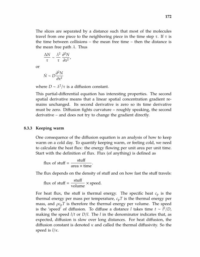
180 180

180 180

172

2010-05-13 00:43:32 / rev b667c9e4c1f1+

The slices are separated by a distance such that most of the moleculestravel from one piece to the neighboring piece in the time step τ. If τ isthe time between collisions – the mean free time – then the distance isthe mean free path λ. Thus

∆Nτ∼λ2

τ∂2N∂x2 ,

or

N ∼ D∂2N∂x2

where D ∼ λ2/τ is a diffusion constant.

This partial-differential equation has interesting properties. The secondspatial derivative means that a linear spatial concentration gradient re-mains unchanged. Its second derivative is zero so its time derivativemust be zero. Diffusion fights curvature – roughly speaking, the secondderivative – and does not try to change the gradient directly.

8.3.3 Keeping warm

One consequence of the diffusion equation is an analysis of how to keepwarm on a cold day. To quantify keeping warm, or feeling cold, we needto calculate the heat flux: the energy flowing per unit area per unit time.Start with the definition of flux. Flux (of anything) is defined as

flux of stuff =stuff

area × time.

The flux depends on the density of stuff and on how fast the stuff travels:

flux of stuff =stuff

volume× speed.

For heat flux, the stuff is thermal energy. The specific heat cp is thethermal energy per mass per temperature, cpT is the thermal energy permass, and ρcpT is therefore the thermal energy per volume. The speedis the ‘speed’ of diffusion. To diffuse a distance l takes time t ∼ l2/D,making the speed l/t or D/l. The l in the denominator indicates that, asexpected, diffusion is slow over long distances. For heat diffusion, thediffusion constant is denoted κ and called the thermal diffusivity. So thespeed is l/κ.

181 181

181 181

173

2010-05-13 00:43:32 / rev b667c9e4c1f1+

Combine the thermal energy per volume with the diffusion speed:

thermal flux = ρcpT × κl.

∆x

T1

T2

The product ρcpκ occurs so frequently that it is givena name: the thermal conductivity K. The ratio T/l isa lumped version of the temperature gradient ∆T/∆x.With those substitutions, the thermal flux is

F = K∆T∆x.

With one side held at T1 and the other at T2, the tem-perature gradient is (T2 − T1)/∆x.

To estimate how much heat one loses on a cold day, we need to estimateK = ρcpκ. To do so, put all the pieces together:

ρ ∼ 1kgm−3,

cp ∼ 103 J kg−1 K−1,

κ ∼ 1.5 ·10−5 m2 s−1,

where we are guessing that κ = ν (because both κ and ν are diffusionconstants). Then

K = ρcpκ ∼ 0.02Wm−1 K−1.

Using this value we can estimate the heat loss on a cold day. Let’s saythat your skin is at T2 = 30 C and the air outside is T1 = 0 C, making∆T = 30K. A thin T-shirt may have thickness 2mm, so

F = K∆T∆x∼ 0.02Wm−1 K−1

×30K

2 ·10−3 m∼ 300Wm−2.

Damn, we want a power rather than a power per area. Ah, flux is powerper area, so just multiply by a person’s surface area: roughly 2m tall and0.5m wide, with a front and a back. So the surface area is about 2m2.Thus, the power lost is

P ∼ FA = 300Wm−2× 2m2 = 600W.

No wonder a winter day wearing only thin pants and shirt feels so cold:600W is large compared to human power levels. Sitting around, a personproduces 100W of heat (the basal metabolic rate). When 600W escapes,

182 182

182 182

174

2010-05-13 00:43:32 / rev b667c9e4c1f1+

one is losing far more than the basal metabolic rate. Eventually, one’score body temperature falls. Then chemical reactions slow down. Thishappens for two reasons. First, almost all reactions go slower at lowertemperature. Second, enzymes lose their optimized shape, so they be-come less efficient. Eventually you die.

One solution is jogging to generate extra heat. That solution indicatesthat the estimate of 600W is plausible. Cycling hard, which generateshundreds of watts of heat, is vigorous enough exercise to keep one warm,even on a winter day in thin clothing.

Another simple solution, as parents repeat to their children: Dress warmlyby putting on thick layers. Let’s recalculate the power loss if you put ona fleece that is 2 cm thick. You could redo the whole calculation fromscratch, but it is simpler is to notice that the thickness has gone up by afactor of 10 but nothing else changed. Because F ∝ 1/∆x, the flux and thepower drop by a factor of 10. So, wearing the fleece makes

P ∼ 60W.

That heat loss is smaller than the basal metabolic rate, which indicatesthat one would not feel too cold. Indeed, when wearing a thick fleece,only the exposed areas (hands and face) feel cold. Those regions areexposed to the air, and are protected by only a thin layer of still air (theboundary layer). Because a large ∆x means a small heat flux, the moralis (speaking as a parent): Listen to your parents and bundle up!

183 183

183 1832010-05-13 00:43:32 / rev b667c9e4c1f1+

9Springs

9.1 Why planets orbit in ellipses 1759.2 Musical tones 1819.3 Waves 1879.4 Precession of planetary orbits 229

Almost every physical process contains a spring! The first example ofthat principle shows a surprising place for a spring: planetary orbits.

9.1 Why planets orbit in ellipses

For a planet moving around the sun (assumed to be infinitely massive),the planet’s energy per mass is

Em

= −GM

r+

12

v2, (9.1)

where m is the mass of the planet, G is Newton’s constant, M is the massof the sun, r is the planet’s distance from the sun, and v is the planet’sspeed.

sun

planet

r

θ

In polar coordinates, the kinetic energy per mass is

12

v2 =12

r2(dθdt

)2

+

(drdt

)2 . (9.2)

This energy contains two coordinates, which is onetoo many for an easy solution. We can get rid ofa coordinate by incorporating a conservation law,

184 184

184 184

176

2010-05-13 00:43:32 / rev b667c9e4c1f1+

angular momentum. The angular momentum permass is

` = r2 dθdt, (9.3)

The angular momentum per mass ` allow us to eliminate the θ coordinateby rewriting the dθ

dt term:

r2(dθdt

)2

=`2

r2 . (9.4)

Therefore,

12

v2 =12

`2

r2 +

(drdt

)2 ; (9.5)

and

Em

= −GM

r+

12`2

r2︸ ︷︷ ︸Veff

+12

(drdt

)2

︸ ︷︷ ︸KE per mass

. (9.6)

Because the gravitational force is central (toward the sun), the planet’s an-gular momentum, when computed about the sun, is constant. Therefore,the only variable in E/m is r. This energy per mass describes the motionof a particle in one dimension (r). The first two terms are the potential(the potential energy per mass); they are called the effective potential Veff.The final term is the particle’s kinetic energy per mass.

Veff

r

Now let’s study the just the effective po-tential:

Veff = −GM

r+

12`2

r2 . (9.7)

The first term is the actual gravitationalpotential; the second term, which orig-inated from the tangential motion, is calledthe centrifugal potential. To understandhow they work together, let’s make a sketch. For almost any sketch, thefirst tool to pull out is easy cases. Here, the easy cases are small and larger. At small r, the centrifugal potential is the important term because its

185 185

185 185

177

2010-05-13 00:43:32 / rev b667c9e4c1f1+

1/r2 overwhelms the 1/r in the gravitational potential. At large r, the grav-itational potential is the important term, because its 1/r approaches zeromore slowly than does the 1/r2 in the centrifugal potential. Therefore,

Veff ∝

1/r2 (small r)−1/r (large r) (9.8)

If this analysis and sketch look familiar, that’s because they are. The ef-fective potential has the same form as the energy in hydrogen (Section 7.3or r26-lumping-hydrogen.pdf); therefore, our conclusions about plan-etary motion will generalize to hydrogen.

Veff

r

circular orbit

r0

Imagine the planet orbiting in a circularorbit. In that orbit, r remains constantso dr/dt and d2r/dt2 are both zero. Forthat to be true, the particle must livewhere the effective potential Veff is flat –in other words, at its minimum at r = r0.

Veff

rrmin rmax

Now perturb the orbit by kicking theplanet slightly outwards. That kick doesnot change the angular momentum `,because angular momentum depends onthe tangential velocity. But it gives theplanet a nonzero radial velocity (dr/dt 6=0). Thus, it now has r-coordinate kineticenergy (the θ-coordinate kinetic energyis taken care of by the centrifugal-potentialpiece of the effective potential). The orbital radius r then varies betweenthe extremes where the r kinetic energy turns completely into effective-potential energy. Those are the two points where the horizontal line inter-sects the effective potential, and the corresponding radii are the minimumand maximum orbital distances.

186 186

186 186

178

2010-05-13 00:43:32 / rev b667c9e4c1f1+

Veff

r

But what shape is that orbit? Findingthe shape seemingly requires solving thedifferential equation for r, using the con-servation of angular momentum to finddθ/dt, and then integrating to find θ(t).

An alternative approach is to use theobservation that, near its minimum, theeffective potential is shaped like a parabola.We can find that parabola by expanding Veff in a Taylor series about theminimum. To do so, first find the the minimum-energy radius r0 (theradius of the circular orbit). By setting dVeff/dr = 0, we find

r0 =`2

GM. (9.9)

The Taylor series about r0 is

Veff(r) = Veff(r0) + (r − r0) dVeff

dr

∣∣∣∣∣r=r0

+12

(r − r0)2 d2Veff

dr2

∣∣∣∣∣∣r=r0

+ · · · . (9.10)

The first term in the Taylor series is just a constant, so it has no effect onthe motion of the planet (forces depend on differences in energies, so aconstant offset has no effect). The second term vanishes because at theminimum energy, i.e. where r = r0, the slope of Veff is zero. The third termcontains the interesting physics. To evaluate it, we first need to computethe second derivative:

d2Veff

dr2 = −2GMr3 + 3`

2

r4 . (9.11)

At r = r0, it becomes (after using r0 = `2/GM)

d2Veff

dr2

∣∣∣∣∣∣r=r0

=GMr3

0. (9.12)

Therefore, the Taylor approximation is

Veff = irrelevant constant +12

GMr3

0(r − r0)2. (9.13)

Compare this potential energy per mass to the potential energy (per mass)for a mass on a spring,

187 187

187 187

179

2010-05-13 00:43:32 / rev b667c9e4c1f1+

V =12

km

(x − a)2, (9.14)

where a is the spring’s equilibrium length. The spring and the planethave the same form for the potential energy per mass. One needs onlythe following mapping:

x↔ r.a↔ r0.

k/m↔ GM/r30.

(9.15)

Therefore, like the x coordinate for the mass on the spring, the planet’sdistance to the sun (the r coordinate) oscillates in simple harmonic motion!For the mass on a spring, the angular frequency of oscillation is ω =

√k/m.

Therefore, using the preceding mappings, we find that the planet’s radialdistance oscillates about r0 with angular frequency

ωperturb =

√GMr3

0. (9.16)

The planet’s motion is therefore described by two frequencies. The first isωperturb, the just-computed oscillation frequency of the r coordinate. Thesecond is ωorbit, the oscillation frequency of the orbital motion around thesun (the tangential frequency). Their dimensionless ratio ωperturb/ωorbitdetermines the shape of the orbit. Here are the orbit shapes marked withthe ratio ωperturb/ωorbit, with each orbit drawn against the unperturbedcircular orbit.

sun sunsun sun

1.0 2.0 2.5 3.0

The orbital frequency of the circular orbit is

ωorbit =vr0, (9.17)

where v is the orbital velocity (the tangential velocity). To solve for v/r0,equate the centripetal acceleration to the gravitational acceleration:

188 188

188 188

180

2010-05-13 00:43:32 / rev b667c9e4c1f1+

v2

r0=

GMr2

0. (9.18)

To manufacture v/r0 on the left side, divide both sides by r0 and take thesquare root:

vr0︸︷︷︸ωorbit

=

√GMr3

0. (9.19)

This expression is also ωperturb. Therefore, ωorbit = ωperturb.

sun

This result explains the elliptical (Kepler) orbits. First,the ratio is an integer, so the orbit is closed (compare theorbit with the ratio 2.5) – as it should be. Second, theratio is 1, so the orbit’s center is slightly away from thesun – as it should for a planetary orbit (the sun is at onefocus of the ellipse, not at the center). The surprisingconclusion of all the analysis is that a planetary orbit contains a spring;once this fact is appreciated, a spring analysis allows us to understandthe complicated orbital motion without solving complicated differentialequations.

As a bonus, the effective potential has the same form as the energy inhydrogen. Therefore, that energy also looks like a parabola near its min-imum. The consequence is that a chemical bond acts like a spring (forsmall extensions). This second application is not a mere coincidence.Near a minimum, almost every function looks a parabola, so almost everyphysical system contains a spring. Springs are everywhere!

189 189

189 189

181

2010-05-13 00:43:32 / rev b667c9e4c1f1+

9.2 Musical tones

9.2.1 Wood blocks

Here is a home musical experiment that illustrates proportional reasoningand springs. First construct, or ask a carpenter or a local lumber yard toconstruct, two wood blocks made from the same larger wood plank. Minehave these dimensions:

1. 30 cm × 5 cm × 1 cm; and

2. 30 cm × 5 cm × 2 cm.

The blocks are identical except in their thickness: 2 cm vs 1 cm.

Now tap the thin block at the center while holding it lightlytoward the edge, and listen to the musical note. If you do thesame experiment to the thick block, will the pitch (fundamentalfrequency) be higher than, the same as, or lower than the pitchwhen you tapped the thin block?

You can answer this question in many ways. The first is to dothe experiment. It would be nice either to predict the resultbefore doing the experiment or to explain and understand theresult after doing the experiment.

One argument is that the block is a resonant object, and the wavelengthof the sound depends on the thickness of the block. In that picture, thethick block should have the longer wavelength and therefore the lowerfrequency. A counterargument, based on a different model of how thesound is made, is that the thick block is stiffer, so it vibrates faster. On theother hand, the thick block is more massive, so it vibrates more slowly.Perhaps these two effects – greater stiffness but greater mass – cancel eachother, leaving the frequency unchanged?

I’ll do the experiment right now and tell you the result. The thick blockhas a higher pitch. So the resonant-cavity model is probably wrong.Instead, the stiffness probably more than overcomes the mass.

A spring model explains this result and even predicts the frequency ratio.In the spring model, a wood block is made of wood atoms connected by

190 190

190 190

182

2010-05-13 00:43:32 / rev b667c9e4c1f1+

chemical bonds, which are springs. As the block vibrates, it takes theseshapes (shown in a side view):

The block is made of springs, and it acts like a big spring. The middleposition is the equilibrium position, when the block has zero potentialenergy and maximum kinetic energy. The potential energy is stored instretching and compressing the bonds. Imagine deforming the block intoa shape like the first shape:

Each dot is a wood ‘atom’, and each gray line is a spring that modelsthe chemical bond between wood atoms. Deforming the block stretchesand compresses these bonds. These numerous individual springs com-bine to make the block behave like a large spring. Because the block isa big spring, the energy required to to produce a vertical deflection isproportional to the square of the deflection:

E ∼ ky2, (9.20)

where y is the deflection, and k is the stiffness of the block.

Intuitively, the thicker the block, the stiffer it is (higher k). The springmodel will help us find how k depends on the thickness h. To do so,imagine deflecting the thin and thick blocks by the same distance y, thencompare their stored energies Ethin and Ethick by forming their ratio

Ethick

Ethin. (9.21)

That ratio iskthicky2

kthiny2 =kthickkthin

(9.22)

because y is the same for the thick and thin blocks. So, the ratio of storedenergies is also the ratio of stiffnesses.

191 191

191 191

183

2010-05-13 00:43:32 / rev b667c9e4c1f1+

To find the stored energies, look at this picture of the blocks, with thedotted line showing the neutral line (the line without compression orextension):

y y

The deflection hardly changes the lengths of the radial-direction bondsprings. However, the tangential springs (along the long length of theblock) get extended or compressed. Above the neutral line the springsare extended. Below the neutral line, the springs are compressed. Theamount of extension is proportional to the distance from the neutral line.

Now study comparable bond springs in the thin and thick blocks. Eachspring in the thin block corresponds to a spring in the thick block that istwice as far away from the neutral line. The spring in the thick block hastwice the extension (or compression) of its partner in the thin block. Sothe spring in the thick block stores four times the energy of its partnerspring in the thin block. Furthermore, the thick block has twice as manylayers as does the thin black, so each spring in the thin block has twopartners, with identical extension, in the thick block. So the thick blockstores eight times the energy of the thin block (for the same deflection y).

Thuskthickkthin

= 8. (9.23)

This factor of 8 results from multiplying the thickness by 2. In general,stiffness is proportional to the cube of the thickness:

k ∝ h3. (9.24)

Because the entire wood block acts like a spring, its oscillation frequencyis ω =

√k/m. The mass ratio is caused by the thickness ratio:

mthick

mthin= 2. (9.25)

Because the stiffness ratio is 8, the frequency ratio is

ωthick

ωthin=

√82

= 2. (9.26)

192 192

192 192

184

2010-05-13 00:43:32 / rev b667c9e4c1f1+

In general, m ∝ h so

ωthick

ωthin=

√h3

h= h. (9.27)

Frequency is proportional to thickness!

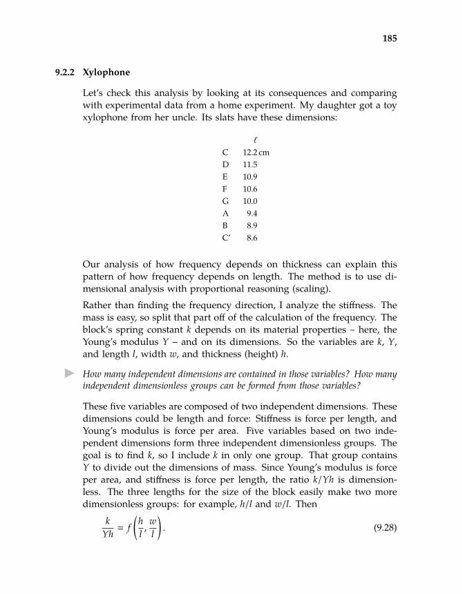
193 193

193 193

185

2010-05-13 00:43:32 / rev b667c9e4c1f1+

9.2.2 Xylophone

Let’s check this analysis by looking at its consequences and comparingwith experimental data from a home experiment. My daughter got a toyxylophone from her uncle. Its slats have these dimensions:

`

C 12.2 cmD 11.5E 10.9F 10.6G 10.0A 9.4B 8.9C’ 8.6

Our analysis of how frequency depends on thickness can explain thispattern of how frequency depends on length. The method is to use di-mensional analysis with proportional reasoning (scaling).

Rather than finding the frequency direction, I analyze the stiffness. Themass is easy, so split that part off of the calculation of the frequency. Theblock’s spring constant k depends on its material properties – here, theYoung’s modulus Y – and on its dimensions. So the variables are k, Y,and length l, width w, and thickness (height) h.

How many independent dimensions are contained in those variables? How manyindependent dimensionless groups can be formed from those variables?

These five variables are composed of two independent dimensions. Thesedimensions could be length and force: Stiffness is force per length, andYoung’s modulus is force per area. Five variables based on two inde-pendent dimensions form three independent dimensionless groups. Thegoal is to find k, so I include k in only one group. That group containsY to divide out the dimensions of mass. Since Young’s modulus is forceper area, and stiffness is force per length, the ratio k/Yh is dimension-less. The three lengths for the size of the block easily make two moredimensionless groups: for example, h/l and w/l. Then

kYh

= f(hl,wl

). (9.28)

194 194

194 194

186

2010-05-13 00:43:32 / rev b667c9e4c1f1+

Guess the function f (except for a dimensionless constant).

What we know about stiffness versus thickness, along with proportionalreasoning, is enough to solve for f , except for a dimensionless constant.Proportional reasoning helps determine the dependence on the dimen-sionless group w/l. Imagine doubling the width w. Equivalently, I gluetogether two identical blocks along the long, thin edge. When the newblock is bent, the individual blocks contains equal energy, so the newblock contains twice the energy of an original block. Therefore, doublingthe width doubles the stiffness; in symbols, k ∝ w. In the general form

kYh

= f(hl,wl

). (9.29)

w appears only in the group w/l, and k appears on the right in the firstpower. So the general form simplifies to

kYh

=wl· f

(hl

). (9.30)

To guess the new function f , I use what I know about stiffness versusthickness, that k ∝ h3. Therefore the left side, k/Yh, is proportional to h2.On the right side the only source of h is from f , which can play with hbut only via the ratio h/l. So

f(hl

)∼

(hl

)2

. (9.31)

Combining these deductions gives

kYh∼

wl

(hl

)2

=wh2

l3(9.32)

and

k ∼ Yw(hl

)3

. (9.33)

The stiffness and mass determine the frequency. The mass is m = ρwlh.So

ω ∼

√km∼

√Yρ

hl2. (9.34)

195 195

195 195

187

2010-05-13 00:43:32 / rev b667c9e4c1f1+

As a quick check, this result is consistent with the earlier calculation thatfrequency is proportional to thickness. And it contains a new result:ω ∝ l−2.

Problem 9.1 Effect of widthIs it physically plausible that the width w does not affect the frequency ω?

Is this data consistent with the prediction that ω ∝ l−2?

` fC 12.2 261.6D 11.5 293.6E 10.9 329.6F 10.6 349.2G 10.0 392.0A 9.4 440.0B 8.9 493.8C’ 8.6 523.2

Before doing an extensive analysis, I check the easycase of the octave. The lower and higher C notesare a factor of 2 apart in frequency. If the scal-ing prediction is correct, the respective slat lengthsshould be a factor of

√2 apart. The length ratio is

12.2/8.6 ∼ 1.419, which is very close to√

2. The gen-eral pattern is that f l2 should be invariant. To check,here is the same table with frequencies, which arecomputed by assuming that the A above middle C isat 440Hz (concert A), and with a column for f l2:

The proposed invariant is, experimentally, almost con-stant.

9.3 Waves

Ocean covers most of the earth, and waves roam most of the ocean. Wavesalso cross puddles and ponds. What makes them move, and what deter-mines their speed? By applying and extending the techniques of approx-imation, we analyze waves. For concreteness, this section refers mostly towater waves but the results apply to any fluid.

9.3.1 Dispersion relations

The most organized way to study waves is to use dispersion relations.A dispersion relation states what values of frequency and wavelength awave can have. Instead of the wavelength λ, dispersion relations usuallyconnect frequency ω, and wavenumber k, which is defined as 2π/λ. Thispreference has an basis in order-of-magnitude reasoning. Wavelength isthe the distance the wave travels in a full period, which is 2π radians of

196 196

196 196

188

2010-05-13 00:43:32 / rev b667c9e4c1f1+

oscillation. Although 2π is dimensionless, it is not the ideal dimensionlessnumber, which is unity. In 1 radian of oscillation, the wave travels adistance

λ ≡λ

2π. (9.35)

The bar notation, meaning ‘divide by 2π’, is chosen by analogy with h and~. The one-radian forms such as ~ are more useful for approximationsthan the 2π-radian forms. The Bohr radius, in a form where the dimen-sionless constant is unity, contains ~ rather than h. Most results withwaves are similarly simpler using λ rather than λ. A further refinementis to use its inverse, the wavenumber k = 1/λ. This choice, which has di-mensions of inverse length, parallels the definition of angular frequencyω, which has dimensions of inverse time. A relation that connects ω andk is likely to be simpler than one connecting ω and λ, although either issimpler than one connecting ω and λ.

The simplest dispersion relation describes electromagnetic waves in a vac-uum. Their frequency and wavenumber are related by the dispersionrelation

ω = ck, (9.36)

which states that waves travel at velocity ω/k = c, independent of fre-quency. Dispersion relations contain a vast amount of information aboutwaves. They contain, for example, how fast crests and troughs travel: thephase velocity. They contain how fast wave packets travel: the groupvelocity. They contain how these velocities depend on frequency: thedispersion. And they contain the rate of energy loss: the attenuation.

9.3.2 Phase and group velocities

The usual question with a wave is how fast it travels. This questionhas two answers, the phase velocity and the group velocity, and bothdepend on the dispersion relation. To get a feel for how to use dispersionrelations (most of the chapter is about how to calculate them), we discussthe simplest examples that illustrate these two velocities. These analysesstart with the general form of a traveling wave:

f (x, t) = cos(kx − ωt), (9.37)

197 197

197 197

189

2010-05-13 00:43:32 / rev b667c9e4c1f1+

where f is its amplitude.00

00

11

11t = t1:

t = t2:

cos(kx−ωt1)

cos(kx−ωt2)

Phase veloc-ity is an eas-ier idea thangroup veloc-ity so, as anexample ofdivide-and-conquer reasoning and of maximal laziness, study it first. Thephase, which is the argument of the cosine, is kx−ωt. A crest occurs whenthe phase is zero. In the top wave, a crest occurs when x = ωt1/k. In thebottom wave, a crest occurs when x = ωt2/k. The difference

ωk

(t2 − t1) (9.38)

is the distance that the crest moved in time t2 − t1. So the phase velocity,which is the velocity of the crests, is

vph =distance crest shifted

time taken=ωk. (9.39)

To check this result, check its dimensions: ω provides inverse time and1/k provides length, so ω/k is a speed.

Group velocity is trickier. The word ‘group’ suggests that the conceptinvolves more than one wave. Because two is the first whole numberlarger than one, the simplest illustration uses two waves. Instead of beinga function relating ω and k, the dispersion relation here is a list of allowed(k, ω) pairs. But that form is just a discrete approximation to an officialdispersion relation, complicated enough to illustrate group velocity andsimple enough to not create a forest of mathematics. So here are twowaves with almost the same wavenumber and frequency:

f1 = cos(kx − ωt),f2 = cos((k + ∆k)x − (ω + ∆ω)t),

(9.40)

where ∆k and ∆ω are small changes in wavenumber and frequency, re-spectively. Each wave has phase velocity vph = ω/k, as long as ∆k and ∆ωare tiny. The figure shows their sum.

198 198

198 198

190

2010-05-13 00:43:32 / rev b667c9e4c1f1+

x

x

x

A

+

B

=

The point of the figure is that two cosines with almost the same spatialfrequency add to produce an envelope (thick line). The envelope itselflooks like a cosine. After waiting a while, each wave changes because ofthe ωt or (ω + ∆ω)t terms in their phases. So the sum and its envelopechange to this:

x

x

x

A

+

B

=

The envelope moves, like the crests and troughs of any wave. It is a wave,so it has a phase velocity, which motivates the following definition:

Group velocity is the phase velocity of the envelope. (9.41)

With this pictorial definition, you can compute group velocity for thewave f1 + f2. As suggested in the figures, adding two cosines produces aa slowly varying envelope times a rapidly oscillating inner function. Thistrigonometric identity gives the details:

cos(A + B) = 2 cos(B − A

2

)︸ ︷︷ ︸

envelope

× cos(A + B

2

)︸ ︷︷ ︸

inner

. (9.42)

If A ≈ B, then A − B ≈ 0, which makes the envelope vary slowly. Applythe identity to the sum:

f1 + f2 = cos(kx − ωt︸ ︷︷ ︸A

) + cos((k + ∆k)x − (ω + ∆ω)t︸ ︷︷ ︸B

). (9.43)

Then the envelope contains

199 199

199 199

191

2010-05-13 00:43:32 / rev b667c9e4c1f1+

cos(B − A

2

)= cos

(x∆k − t∆ω

2

). (9.44)

The envelope represents a wave with phase

∆k2

x − ∆ω2

t. (9.45)

So it is a wave with wavenumber ∆k/2 and frequency ∆ω/2. The enve-lope’s phase velocity is the group velocity of f1 + f2:

vg =frequency

wavenumber=

∆ω/2∆k/2

=∆ω∆k. (9.46)

In the limit where ∆k→ 0 and ∆ω→ 0, the group velocity is

vg =∂ω∂k. (9.47)

It is usually different from the phase velocity. A typical dispersion re-lation, which appears several times in this chapter, is ω ∝ kn. Thenvph = ω/k = kn−1 and vg ∝ nkn−1. So their ratio is

vgvph

= n. (for a power-law relation) (9.48)

Only when n = 1 are the two velocities equal. Now that we can find wavevelocities from dispersion relations, we return to the problem of findingthe dispersion relations.

9.3.3 Dimensional analysis

A dispersion relation usually emerges from solving a wave equation,which is an unpleasant partial differential equation. For water waves,a wave equation emerges after linearizing the equations of hydrodynam-ics and neglecting viscosity. This procedure is mathematically involved,particularly in handling the boundary conditions. Alternatively, you canderive dispersion relations using dimensional analysis, then complete andcomplement the derivation with physical arguments. Such methods usu-ally cannot evaluate the dimensionless constants, but the beauty of study-ing waves is that, as in most problems involving springs and oscillations,most of these constants are unity.

200 200

200 200

192

2010-05-13 00:43:32 / rev b667c9e4c1f1+

How do frequency and wavenumber connect? They have dimensions ofT−1 and L−1, respectively, and cannot form a dimensionless group withouthelp. So include more variables. What physical properties of the systemdetermine wave behavior? Waves on the open ocean behave differentlyfrom waves in a bathtub, perhaps because of the difference in the depthof water h. The width of the tub or ocean could matter, but then theproblem becomes two-dimensional wave motion. In a first analysis, avoidthat complication and consider waves that move in only one dimension,perpendicular to the width of the container. Then the width does notmatter.

To determine what other variables are important, use the principle thatwaves are like springs, because every physical process contains a spring.This blanket statement cannot be strictly correct. However, it is useful asa broad generalization. To get a more precise idea of when this assump-tion is useful, consider the characteristics of spring motion. First, springshave an equilibrium position. If a system has an undisturbed, restingstate, consider looking for a spring. For example, for waves on the ocean,the undisturbed state is a calm, flat ocean. For electromagnetic waves –springs are not confined to mechanical systems – the resting state is anempty vacuum with no radiation. Second, springs oscillate. In mechani-cal systems, oscillation depends on inertia to carry the mass beyond theequilibrium position. Equivalently, it depends on kinetic energy turninginto potential energy, and vice versa. Water waves store potential energyin the disturbance of the surface and kinetic energy in the motion of thewater. Electromagnetic waves store energy in the electric and magneticfields. A magnetic field is generated by moving or spinning charges, sothe magnetic field is a reservoir of kinetic (motion) energy. An electricfield is generated by stationary charges and has an associated potential,so the electric field is the reservoir of potential energy. With these identi-fications, the electromagnetic field acts like a set of springs, one for eachradiation frequency. These examples are positive examples. A negativeexample – a marble oozing its way through glycerin – illustrates thatsprings are not always present. The marble moves so slowly that the ki-netic energy of the corn syrup, and therefore its inertia, is miniscule andirrelevant. This system has no reservoir of kinetic energy, for the kineticenergy is merely dissipated, so it does not contain a spring.

201 201

201 201

193

2010-05-13 00:43:32 / rev b667c9e4c1f1+

Waves have the necessary reservoirsto act like springs. The surface of wa-ter is flat in its lowest-energy state.Deviations, also known as waves, areopposed by a restoring force. Dis-torting the surface is like stretching arubber sheet: Surface tension resiststhe distortion. Distorting the surfacealso requires raising the average wa-ter level, a change that gravity resists.

The average height of the surface doesnot change, but the average depth ofthe water does. The higher column, under the crest, has more waterthan the lower column, under the trough. So in averaging to find theaverage depth, the higher column gets a slightly higher weighting. Thusthe average depth increases. This result is consistent with experience: Ittakes energy to make waves.

The total restoring force includes gravity and surface tension so, in thelist of variables, include surface tension (γ) and gravity (g).

In a wave, like in a spring, the restoring force fights inertia, representedhere by the fluid density. The gravitational piece of the restoring forcedoes not care about density: Gravity’s stronger pull on denser substancesis exactly balanced by their greater inertia. This exact cancellation is a re-statement of the equivalence principle, on which Einstein based the theoryof general relativity [4, 5]. In pendulummotion, the mass of the bob dropsout of the final solution for the same reason. The surface-tension piece ofthe restoring force, however, does not change when density changes. Thesurface tension itself, the fluid property γ, depends on density because itdepends on the spacing of atoms at the surface. That dependence affectsγ. However, once you know γ you can compute surface-tension forceswithout knowing the density. Since ρ does not affect the surface-tensionforce but affects the inertia, it affects the properties of waves in whichsurface tension provides a restoring force. Therefore, include ρ in the list.

202 202

202 202

194

2010-05-13 00:43:32 / rev b667c9e4c1f1+

Var Dim Whatω T−1 frequencyk L−1 wavenumberg LT−2 gravityh L depthρ ML−3 densityγ MT−2 surface tension

To simplify the analysis, assume that the wavesdo not lose energy. This choice excludes viscos-ity from the set of variables. To further simplify,exclude the speed of sound. This approxima-tion means ignoring sound waves, and is validas long as the flow speeds are slow compared tothe speed of sound. The resulting ratio,

M ≡flow speedsound speed

, (9.49)

is dimensionless and, because of its importance, is given a name: theMach number. Finally, assume that the wave amplitude ξ is small com-pared to its wavelength and to the depth of the container. The table showsthe list of variables. Even with all these restrictions, which significantlysimplify the analysis, the results explain many phenomena in the world.

These six variables built from three fundamental dimensions producethree dimensionless groups. One group is easy: the wavenumber k is aninverse length and the depth h is a length, so

Π1 ≡ kh. (9.50)

This group is the dimensionless depth of the water: Π1 1 means shal-low and Π1 1 means deep water. A second dimensionless group comesfrom gravity. Gravity, represented by g, has the same dimensions as ω2,except for a factor of length. Dividing by wavenumber fixes this deficit:

Π2 =ω2

gk. (9.51)

Without surface tension, Π1 and Π2 are the only dimensionless groups,and neither group contains density. This mathematical result has a physi-cal basis. Without surface tension, the waves propagate because of gravityalone. The equivalence principle says that gravity affects motion indepen-dently of density. Therefore, density cannot – and does not – appear ineither group.

Now let surface tension back into the playpen of dimensionless groups.It must belong in the third (and final) group Π3. Even knowing that γbelongs to Π3 still leaves great freedom in choosing its form. The usualpattern is to find the group and then interpret it, as we did for Π1 and

203 203

203 203

195

2010-05-13 00:43:32 / rev b667c9e4c1f1+

Π2. Another option is to begin with a physical interpretation and use theinterpretation to construct the group. Here you can construct Π3 to mea-sure the relative importance of surface-tension and gravitational forces.Surface tension γ has dimensions of force per length, so producing a forcerequires multiplying by a length. The problem already has two lengths:wavelength (represented via k) and depth. Which one should you use?The wavelength probably always affects surface-tension forces, becauseit determines the curvature of the surface. The depth, however, affectssurface-tension forces only when it becomes comparable to or smaller thanthe wavelength, if even then. You can use both lengths to make γ into aforce: for example, F ∼ γ

√h/k. But the analysis is easier if you use only

one, in which case the wavelength is the preferable choice. So Fγ ∼ γ/k.Gravitational force, also known as weight, is ρg × volume. Following theprecedent of using only k to produce a length, the gravitational force isFg ∼ ρg/k3. The dimensionless group is then the ratio of surface-tensionto gravitational forces:

Π3 ≡FγFg

=γ/kρg/k3 =

γk2

ρg. (9.52)

This choice has, by construction, a useful physical interpretation, butmany other choices are possible. You can build a third group withoutusing gravity: for example, Π3 ≡ γk3/ρω2. With this choice, ω appearsin two groups: Π2 and Π3. So it will be hard to solve for it. The choicemade for P3, besides being physically useful, quarantines ω in one group:a useful choice since ω is the goal.

Now use the groups to solve for frequency ω as a function of wavenumberk. You can instead solve for k as a function of ω, but the formulas forphase and group velocity are simpler with ω as a function of k. Only thegroup Π2 contains ω, so the general dimensionless solution is

Π2 = f (Π1,Π3), (9.53)

orω2

gk= f

(kh,

γk2

ρg

). (9.54)

Then

ω2 = gk · f (kh,γk2

ρg). (9.55)

204 204

204 204

196

2010-05-13 00:43:32 / rev b667c9e4c1f1+

This relation is valid for waves in shallow or deep water (small or largeΠ1); for waves propagated by gravity or by surface tension (small or largeΠ3); and for waves in between.

10−4 10−2 102 104Π1 ≡ hk

10−4

10−2

102

104

Π3 ≡γk2

ρg

Deep waterSurface tension

Deep waterGravity

Shallow waterSurface tension

Shallow waterGravity

The figure shows how the two groups Π1 and Π3 divide the world ofwaves into four regions. We study each region in turn, and combinethe analyses to understand the whole world (of waves). The group Π1measures the depth of the water: Are the waves moving on a puddle oran ocean? The group Π3 measures the relative contribution of surfacetension and gravity: Are the waves ripples or gravity waves?

The division into deep and shallow water (left and right sides) followsfrom the interpretation of Π1 = kh as dimensionless depth. The divi-sion into surface-tension- and gravity-dominated waves (top and bottomhalves) is more subtle, but is a result of how Π3 was constructed. As acheck, look at Π3. Large g or small k result in the same consequence: smallΠ3. Therefore the physical consequence of longer wavelength (smaller k)is similar to that of stronger gravity. So longer-wavelength waves are

205 205

205 205

197

2010-05-13 00:43:32 / rev b667c9e4c1f1+

gravity waves. The large-Π3 portion of the world (top half) is thereforelabeled with surface tension.

The next figure shows how wavelength and depth (instead of the dimen-sionless groups) partition the world, and plots examples of different typesof waves.

Π1 = 1

Π3 = 1

10−4 10−2 102 104depth (m)

10−4

10−2

102

104

106

wavelength (m)

TideTide

Storm wave at seaStorm wave at sea

Storm wave at shoreStorm wave at shore

Ripple on pondRipple on pondRipple on thin puddleRipple on thin puddle

Deep waterGravity waves

Shallow waterGravity waves

Deep waterRipples

Shallow-waterRipples

The thick dividing lines are based on the dimensionless groups Π1 = hkand Π3 = γk2/ρg. Each region contains one or two examples of its kindof waves. With g = 1000 cm s−1 and ρ ∼ 1g cm−3, the border wavelengthbetween ripples and gravity waves is just over λ ∼ 1 cm (the horizontal,Π3 = 1 dividing line).

The magic function f is still unknown to us. To determine its form andto understand its consequences, study f in limiting cases. Like a jigsaw-puzzle-solver, study first the corners of the world, where the physics issimplest. Then connect the corner solutions to get solutions valid alongan edge, where the physics is the almost as simple as in a corner. Fi-nally, crawl inward to assemble the complicated, complete solution. Thisextended example illustrates divide-and-conquer reasoning, and usinglimiting cases to choose pieces into which you break the problem.

206 206

206 206

198

2010-05-13 00:43:32 / rev b667c9e4c1f1+

9.3.4 Deep water

10−4 10−2 102 104Π1 ≡ hk

10−4

10−2

102

104

Π3 ≡γk2

ρg

Deep waterSurface tension

Deep waterGravity

Shallow waterSurface tension

Shallow waterGravity

First study deep water, where kh1, as shaded in the map. Deep wa-ter is defined as water sufficientlydeep that waves cannot feel the bot-tom of the ocean. How deep dowaves’ feelers extend? The only lengthscale in the waves is the wavelength,λ = 2π/k. The feelers therefore ex-tend to a depth d ∼ 1/k (as always,neglect constants, such as 2π). Thiseducated guess has a justificationin Laplace’s equation, which is thespatial part of the wave equation.Suppose that the waves are periodicin the x direction, and z measures depth below the surface, as shown inthis figure:

y

x

z

w

λ 2λ

h

Then, Laplace’s equation becomes

∂2φ

∂x2 +∂2φ

∂z2 = 0, (9.56)

where φ is the velocity potential. The ∂2φ/∂y2 term vanishes becausenothing varies along the width (the y direction).

207 207

207 207

199

2010-05-13 00:43:32 / rev b667c9e4c1f1+

It’s not important what exactly φ is. You can find out more about it inan excellent fluid-mechanics textbook, Fluid Dynamics for Physicists [6];Lamb’s Hydrodynamics [14]is a classic but difficult. For this argument, allthat matters is that φ measures the effect of the wave and that φ satisfiesLaplace’s equation. The wave is periodic in the x direction, with a formsuch as sin kx. Take

φ ∼ Z(z) sin kx. (9.57)

The function Z(z) measures how the wave decays with depth.

The second derivative in x brings out two factors of k, and a minus sign:

∂2φ

∂x2 = −k2φ. (9.58)

In order that this φ satisfy Laplace’s equation, the z-derivative term mustcontribute +k2φ. Therefore,

∂2φ

∂z2 = k2φ, (9.59)

so Z(z) ∼ e±kz. The physically possible solution – the one that does notblow up exponentially at the bottom of the ocean – is Z(z) ∼ e−kz. There-fore, relative to the effect of the wave at the surface, the effect of the waveat the bottom of the ocean is ∼ e−kh. When kh 1, the bottom might aswell be on the moon because it has no effect. The dimensionless factor kh– it must be dimensionless to sit alone in an exponent – compares waterdepth with feeler depth d ∼ 1/k:

water depthfeeler depth

∼h

1/k= hk, (9.60)

which is the dimensionless group Π1.

In deep water, where the bottom is hidden from the waves, the waterdepth h does not affect their propagation, so h disappears from the listof relevant variables. When h goes, so does Π1 = kh. There is one caveat.If Π1 is the only group that contains k, then you cannot blithely discardΠ1 just because you no longer care about h. If you did, you would bediscarding k and h, and make it impossible to find a dispersion relation(which connects ω and k). Fortunately, k appears in Π3 = γk2/ρg as wellas in Π1. So in deep water it is safe to discard Π1. This argument for theirrelevance of h is a physical argument. It has a mathematical equivalent

208 208

208 208

200

2010-05-13 00:43:32 / rev b667c9e4c1f1+

in the language of dimensionless groups and functions. Because h hasdimensions, the statement that ‘h is large’ is meaningless. The question is,‘large compared to what length?’ With 1/k as the standard of comparisonthe meaningless ‘h is large’ statement becomes ‘kh is large.’ The productkh is the dimensionless group Π1. Mathematically, you are assuming thatthe function f (kh, γk2/ρg) has a limit as kh→∞.Without Π1, the general dispersion relation simplifies to

ω2 = gk fdeep(γk2

ρg

). (9.61)

This relation describes the deep-water edge of the world of waves. Theedge has two corners, labeled by whether gravity or surface tension pro-vides the restoring force. Although the form of fdeep is unknown, it is asimpler function than the original f , a function of two variables. To deter-mine the form of fdeep, continue the process of dividing and conquering:Partition deep-water waves into its two limiting cases, gravity waves andripples.

9.3.5 Gravity waves on deep water

10−4 10−2 102 104Π1 ≡ hk

10−4

10−2

102

104

Π3 ≡γk2

ρg

Deep waterSurface tension

Deep waterGravity

Shallow waterSurface tension

Shallow waterGravity

Of the two extremes, gravity wavesare the more common. They in-clude wakes generated by ships andmost waves generated by wind. Sospecialize to the corner of the waveworld where water is deep and grav-ity is strong. With gravity muchstronger than surface tension, thedimensionless group Π3 = γk2/ρglimits to 0. Since Π3 is the productof several factors, you can achievethe limit in several ways:

1. Increase g (which is downstairs)by moving to Jupiter.

2. Reduce γ (which is upstairs) by dumping soap on the water.3. Reduce k (which is upstairs) by studying waves with a huge wave-

length.

209 209

209 209

201

2010-05-13 00:43:32 / rev b667c9e4c1f1+

In this limit, the general deep-water dispersion relation simplifies to

ω2 = fdeep(0)gk = C1gk, (9.62)

where fdeep(0) is an as-yet-unknown constant, C1. The use of fdeep(0) as-sumes that fdeep(x) has a limit as x→ 0. The slab argument, which followsshortly, shows that it does. For now, in order to make progress, assumethat it has a limit. The constant remains unknown to the lazy methods ofdimensional analysis, because the methods sacrifice evaluation of dimen-sionless constants to gain comprehension of physics. Usually assume thatsuch constants are unity. In this case, we get lucky: An honest calculationproduces C1 = 1 and

ω2 = 1×gk, (9.63)

where the red 1× indicates that it is obtained from honest physics.

Such results from dimensional analysis seem like rabbits jumping from ahat. The dispersion relation is correct, but your gut may grumble aboutthis magical derivation and ask, ‘But why is the result true?’ A physicalmodel of the forces or energies that drive the waves explains the originof the dispersion relation. The first step is to understand the mechanism:How does gravity make the water level rise and fall? Taking a hint fromthe Watergate investigators,1 we follow the water. The water in the crestdoes not move into the trough. Rather, the water in the crest, beinghigher, creates a pressure underneath it higher than that of the water inthe trough, as shown in this figure:

p> ∼ p0 + ρg(z+ ξ)p> ∼ p0 + ρg(z+ ξ) p< ∼ p0 + ρg(z− ξ)p< ∼ p0 + ρg(z− ξ)

z+ ξ

z− ξ

Flow===⇒

p0 =1atm

When the reporters Woodward and Bernstein [2]were investigating criminal coverups during1the Nixon administration, they received help from the mysterious ‘Deep Throat’, whosevaluable advice was to ‘follow the money.’

210 210

210 210

202

2010-05-13 00:43:32 / rev b667c9e4c1f1+

The higher pressure forces water underneath the crest to flow towardthe trough, making the water level there rise. Like a swing sliding pastequilibrium, the surface overshoots the equilibrium level to produce anew crest and the cycle repeats.

The next step is to quantify the model by estimating sizes, forces, speeds,and energies. In Section 7.1 we analyzed a messy mortality curve byreplacing it with a more tractable shape: a rectangle. The method oflumping worked there, so try it again. ‘A method is a trick I use twice.’—George Polyà. Water just underneath the surface moves quickly becauseof the pressure gradient. Farther down, it moves more slowly. Deep downit does not move at all. Replace this smooth falloff with a step function:Pretend that water down to a certain depth moves as a block, while deeperwater stays still:

w

1/k

1/k

Atop ∼w/k

Lowerpressure

Higherpressure

How deep should this slab of water extend? By the Laplace-equationargument, the pressure variation falls off exponentially with depth, withlength scale 1/k. So assume that the slab has a similar length scale, thatit has depth 1/k. What choice do you have? On an infinitely deep ocean,the only length scale is 1/k. How long should the slab be? Its lengthshould be roughly the peak-to-trough distance of the wave because thesurface height changes significantly over that distance. This distance is1/k. Actually, it is π/k (one-half of a period), but ignore constants. Allthe constants combine into a giant constant at the end, which dimensional

211 211

211 211

203

2010-05-13 00:43:32 / rev b667c9e4c1f1+

analysis cannot determine anyway, so discard it now! The slab’s width wis arbitrary and cancels by the end of any analysis.

So the slab of water has depth 1/k, length 1/k, and width w. Estimate theforces acting on it by estimating the pressure gradients. Across the widthof the slab (the y direction), the water surface is level, so the pressure isconstant along the width. Into the depths (the z direction), the pressurevaries because of gravity – the ρgh term from hydrostatics – but thatvariation is just sufficient to prevent the slab from sinking. We care aboutonly the pressure difference across the length, the direction that the wavemoves. This pressure difference depends on the height of the crest, ξ andis ∆p ∼ ρgξ. This pressure difference acts on a cross-section with areaA ∼ w/k to produce a force

F ∼ w/k︸︷︷︸area

× ρgξ︸︷︷︸∆p

= ρgwξ/k. (9.64)

The slab has mass

m = ρ × w/k2︸︷︷︸volume

, (9.65)

so the force produces an acceleration

aslab ∼ρgwξ

k︸︷︷︸force

/ ρwk2︸︷︷︸mass

= gξk. (9.66)

The factor of g says that the gravity produces the acceleration. Full grav-itational acceleration is reduced by the dimensionless factor ξk, which isroughly the slope of the waves.

The acceleration of the slab determines the acceleration of the surface. Ifthe slab moves a distance x, it sweeps out a volume of water V ∼ xA. Thiswater moves under the trough, and forces the surface upward a distanceV/Atop. Because Atop ∼ A (both are ∼ w/k), the surface moves the samedistance x that the slab moves. Therefore, the slab’s acceleration aslabequals the acceleration a of the surface:

a ∼ aslab ∼ gξk. (9.67)

212 212

212 212

204

2010-05-13 00:43:32 / rev b667c9e4c1f1+

This equivalence of slab and surface acceleration does not hold in shallowwater, where the bottom at depth h cuts off the slab before 1/k; that storyis told in Section 9.3.12.

The slab argument is supposed to justify the deep-water dispersion re-lation derived by dimensional analysis. That relation contains frequencywhereas acceleration relation does not. So massage it until ω appears.The acceleration relation contains a and ξ, whereas the dispersion rela-tion does not. An alternative expression for the acceleration might makethe acceleration relation more like the dispersion relation. With luck theexpression will contain ω2, thereby producing the hoped-for ω2; as abonus, it will contain ξ to cancel the ξ in the acceleration relation.

In simple harmonic motion (springs!), acceleration is a ∼ ω2ξ, where ξ isthe amplitude. In waves, which behave like springs, a is given by the sameexpression. Here’s why. In time τ ∼ 1/ω, the surface moves a distanced ∼ ξ, so a/ω2

∼ ξ and a ∼ ω2ξ. With this replacement, the accelerationrelation becomes

ω2ξ︸︷︷︸a

∼ gξk, (9.68)

or

ω2 = 1×gk, (9.69)

which is the longed-for dispersion relation with the correct dimensionlessconstant in red.

An exact calculation confirms the usual hope that the missing dimension-less constants are close to unity, or are unity. This fortune suggests thatthe procedures for choosing how to measure the lengths were reasonable.The derivation depended on two choices:

1. Replacing an exponentially falling variation in velocity potential by astep function with size equal to the length scale of the exponentialdecay.

2. Taking the length of the slab to be 1/k instead of π/k. This choice usesonly 1 radian of the cycle as the characteristic length, instead of usinga half cycle or π radians. Since 1 is a more natural dimensionlessnumber than π is, choosing 1 radian rather than π or 2π radians oftenimproves approximations.

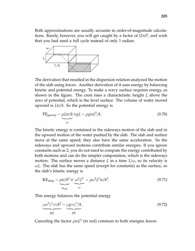
213 213

213 213

205

2010-05-13 00:43:32 / rev b667c9e4c1f1+

Both approximations are usually accurate in order-of-magnitude calcula-tions. Rarely, however, you will get caught by a factor of (2π)6, and wishthat you had used a full cycle instead of only 1 radian.

w

ξ

1/k

The derivation that resulted in the dispersion relation analyzed the motionof the slab using forces. Another derivation of it uses energy by balancingkinetic and potential energy. To make a wavy surface requires energy, asshown in the figure. The crest rises a characteristic height ξ above thezero of potential, which is the level surface. The volume of water movedupward is ξw/k. So the potential energy is

PEgravity ∼ ρξw/k︸︷︷︸m

×gξ ∼ ρgwξ2/k. (9.70)

The kinetic energy is contained in the sideways motion of the slab and inthe upward motion of the water pushed by the slab. The slab and surfacemove at the same speed; they also have the same acceleration. So thesideways and upward motions contribute similar energies. If you ignoreconstants such as 2, you do not need to compute the energy contributed byboth motions and can do the simpler computation, which is the sidewaysmotion. The surface moves a distance ξ in a time 1/ω, so its velocity isωξ. The slab has the same speed (except for constants) as the surface, sothe slab’s kinetic energy is

KEdeep ∼ ρw/k2︸︷︷︸mslab

× ω2ξ2︸︷︷︸v2

∼ ρω2ξ2w/k2. (9.71)

This energy balances the potential energy

ρω2ξ2w/k2︸ ︷︷ ︸KE

∼ ρgwξ2/k︸ ︷︷ ︸PE

. (9.72)

Canceling the factor ρwξ2 (in red) common to both energies leaves

214 214

214 214

206

2010-05-13 00:43:32 / rev b667c9e4c1f1+

ω2∼ gk. (9.73)

The energy method agrees with the force method, as it should, becauseenergy can be derived from force by integration. The energy derivationgives an interpretation of the dimensionless group Π2:

Π2 ∼kinetic energy in slab

gravitational potential energy∼ω2

gk. (9.74)

The gravity-wave dispersion relation ω2 = gk is equivalent to Π2 ∼ 1, or tothe assertion that kinetic and gravitational potential energy are compara-ble in wave motion. This rough equality is no surprise because waves arelike springs. In spring motion, kinetic and potential energies have equalaverages, a consequence of the virial theorem.

The dispersion relation was derived in three ways: by dimensional analy-sis, energy, and force. Using multiple methods increases our confidencenot only in the result but also in the methods. ‘I have said it thrice: WhatI tell you three times is true.’–Lewis Carroll, Hunting of the Snark.

We gain confidence in the methods of dimensional analysis and in theslab model for waves. If we study nonlinear waves, for example, wherethe wave height is no longer infinitesimal, we can use the same techniquesalong with the slab model with more confidence.

With reasonable confidence in the dispersion relation, it’s time study itsconsequences: the phase and group velocities. The crests move at thephase velocity: vph = w/k. For deep-water gravity waves, this velocitybecomes

vph =

√gk, (9.75)

or, using the dispersion relation to replace k by ω,

vph =gω. (9.76)

Let’s check upstairs and downstairs. Who knows where ω belongs, but gdrives the waves so it should and does live upstairs.

In an infinite, single-frequency wave train, the crests and troughs moveat the phase speed. However, a finite wave train contains a mixture of

215 215

215 215

207

2010-05-13 00:43:32 / rev b667c9e4c1f1+

frequencies, and the various frequencies move at different speeds as givenby

vph =gω. (9.77)

Deep water is dispersive. Dispersion makes a finite wave train travel withthe group velocity, given by vg = ∂w/∂k, as explained in Section 9.3.2. Thegroup velocity is

vg =∂∂k

√gk =

12

√gk

=12

vph. (9.78)

So the group velocity is one-half of the phase velocity, as the result forpower-law dispersion relation predicts. Within a wave train, the crestsmove at the phase velocity, twice the group velocity, shrinking and grow-ing to fit under the slower-moving envelope.

An everyday consequence is that ship wakes trail the ship. A ship movingwith velocity v creates gravity waves with vph = v. The waves combineto produce wave trains that propagate forward with the group velocity,which is only vph/2 = v/2. From the ship’s point of view, these gravitywaves travel backward. In fact, they form a wedge, and the opening angleof the wedge depends on the one-half that arises from the exponent.

9.3.6 Surfing

Let’s apply the dispersion relation to surfing. Following one winter stormreported in the Los Angeles Times – the kind of storm that brings cries of‘Surf’s up!’ – waves arrived at Los Angeles beaches roughly every 18 s.How fast were the storm winds that generated the waves? Wind pushesthe crests as long as they move more slowly than the wind. After a long-enough push, the crests move with nearly the wind speed. Thereforethe phase velocity of the waves is an accurate approximation to the windspeed.

The phase velocity is g/ω. In terms of the wave period T, this velocity isvph = gT/2π, so

vwind ∼ vph ∼

g︷ ︸︸ ︷10ms−2

×

T︷︸︸︷18 s

2 × 3∼ 30ms−1. (9.79)

216 216

216 216

208

2010-05-13 00:43:32 / rev b667c9e4c1f1+

In units more familiar to Americans, this wind speed is 60mph, which isa strong storm: about 10 on the Beaufort wind scale (‘whole gale/storm’).The wavelength is given by

λ = vphT ∼ 30ms−1× 18 s ∼ 500m. (9.80)

On the open ocean, the crests are separated by half a kilometer. Nearshore they bunch up because they feel the bottom; this bunching is aconsequence of the shallow-water dispersion relation, the topic of Sec-tion 9.3.13.

In this same storm, the waves arrived at 17 s intervals the following day:a small decrease in the period. Before racing for the equations, first checkthat this decrease in period is reasonable. This precaution is a sanitycheck. If the theory is wrong about a physical effect as fundamentalas a sign – whether the period should decrease or increase – then itneglects important physics. The storm winds generate waves of differentwavelengths and periods, and the different wavelengths sort themselvesduring the trip from the far ocean to Los Angeles. Group and phasevelocity are proportional to 1/ω, which is proportional to the period. Solonger-period waves move faster, and the 18 s waves should arrive beforethe 17 s waves. They did! The decline in the interval allows us to calculatethe distance to the storm. In their long journey, the 18 s waves raced 1 dayahead of the 17 s waves. The ratio of their group velocities is

velocity(18 s waves)velocity(17 s waves)

=1817

= 1 +1

17. (9.81)

so the race must have lasted roughly t ∼ 17days ∼ 1.5 · 106 s. The wavetrain moves at the group velocity, vg = vph/2 ∼ 15ms−1, so the stormdistance was d ∼ tvg ∼ 2 · 104 km, or roughly halfway around the world,an amazingly long and dissipation-free journey.

217 217

217 217

209

2010-05-13 00:43:32 / rev b667c9e4c1f1+

USALALA

stormstorm

t ∼ 17days

9.3.7 Speedboating

Our next application of the dispersion relation is to speedboating: Howfast can a boat travel? We exclude hydroplaning boats from our analysis(even though some speedboats can hydroplane). Longer boats generallymove faster than shorter boats, so it is likely that the length of the boat, l,determines the top speed. The density of water might matter. However,v (the speed), ρ, and l cannot form a dimensionless group. So look foranother variable. Viscosity is irrelevant because the Reynolds number forboat travel is gigantic. Even for a small boat of length 5m, creeping alongat 2ms−1,

Re ∼ 500 cm × 200 cm s−1

10−2 cm2 s−1 ∼ 107. (9.82)

At such a huge Reynolds number, the flow is turbulent and nearly in-dependent of viscosity (Section 6.3.1). Surface tension is also irrelevant,because boats are much longer than a ripple wavelength (roughly 1 cm).The search for new variables is not meeting with success. Perhaps gravityis relevant. The four variables v, ρ, g, and l, build from three dimensions,produce one dimensionless group: v2/gl, also called the Froude number:

Fr ≡ v2

gl. (9.83)

The critical Froude number, which determines the maximum boat speed,is a dimensionless constant. As usual, we assume that the constant isunity. Then the maximum boating speed is:

218 218

218 218

210

2010-05-13 00:43:32 / rev b667c9e4c1f1+

v ∼√

gl. (9.84)

A rabbit has jumped out of our hat. What physical mechanism justi-fies this dimensional-analysis result? Follow the waves as a boat plowsthrough water. The moving boat generates waves (the wake), and it rideson one of those waves. Take the bow wave: It is a gravity wave withvph ∼ vboat. Because v2

ph = ω2/k2, the dispersion relation tells us that

v2boat ∼

ω2

k2 =gk

= gλ, (9.85)

where λ ≡ 1/k = λ/2π. So the wavelength of the waves is roughly v2boat/g.

The other length in this problem is the boat length; so the Froude numberhas this interpretation:

Fr =v2boat/g

l∼

wavelength of bow wavelength of boat

. (9.86)

Why is Fr ∼ 1 the critical number, the assumption in finding the maxi-mum boat speed? Interesting and often difficult physics occurs when adimensionless number is near unity. In this case, the physics is as fol-lows. The wave height changes significantly in a distance λ; if the boat’slength l is comparable to λ, then the boat rides on its own wave and tiltsupward. Tilting upward, it presents a large cross-section to the water,and the drag becomes huge. [Catamarans and hydrofoils skim the water,so this kind of drag does not limit their speed. The hydrofoil makes amuch quicker trip across the English channel than the ferry makes, eventhough the hydrofoil is much shorter.] So the top speed is given by

vboat ∼√

gl. (9.87)

For a small motorboat, with length l ∼ 5m, this speed is roughly 7ms−1,or 15mph. Boats (for example police boats) do go faster than the nominaltop speed, but it takes plenty of power to fight the drag, which is whypolice boats have huge engines.

The Froude number in surprising places. It determines, for example,the speed at which an animal’s gait changes from a walk to a trot or, foranimals that do not trot, to a run. In Section 9.3.7 it determines maximumboating speed. The Froude number is a ratio of potential energy to kineticenergy, as massaging the Froude number shows:

219 219

219 219

211

2010-05-13 00:43:32 / rev b667c9e4c1f1+

Fr =v2

gl=

mv2

mgl∼

kinetic energypotential energy

. (9.88)

Here the massage technique was multiplication by unity (in red). In thisexample, the length l is a horizontal length, so gl is not a gravitationalenergy, but it has a similar structure and in other examples often has aneasy interpretation as gravitational energy.

9.3.8 Walking

In the Froude number for walking speed, l is leg length, and gl is apotential energy. For a human with leg length l ∼ 1m, the conditionFr ∼ 1 implies that v ∼ 3ms−1 or 6mph. This speed is a rough estimatefor the top speed for a race walker. The world record for men’s racewalking was once held by Bernado Segura of Mexico. He walked 20kmin 1h:17m:25.6s, for a speed of 4.31ms−1.

This example concludes the study of gravity waves on deep water, whichis one corner of the world of waves.

9.3.9 Ripples on deep water

10−4 10−2 102 104Π1 ≡ hk

10−4

10−2

102

104

Π3 ≡γk2

ρg

Deep waterSurface tension

Deep waterGravity

Shallow waterSurface tension

Shallow waterGravity

For small wavelengths (large k), sur-face tension rather than gravity pro-vides the restoring force. This choicebrings us to the shaded corner ofthe figure. If surface tension ratherthan gravity provides the restoringforce, then g vanishes from the finaldispersion relation. How to get ridof g and find the new dispersion re-lation? You could follow the samepattern as for gravity waves (Sec-tion 9.3.5). In that situation, the sur-face tension γ was irrelevant, so wediscarded the group Π3 ≡ γk2/ρg.Here, with g irrelevant you might try the same trick: Π3 contains g sodiscard it. In that argument lies infanticide, because it also throws out thephysical effect that determines the restoring force, namely surface tension.

220 220

220 220

212

2010-05-13 00:43:32 / rev b667c9e4c1f1+

To retrieve the baby from the bathwater, you cannot throw out γk2/ρg di-rectly. Instead you have to choose the form of the dimensionless functionfdeep in so that only gravity vanishes from the dispersion relation.

The deep-water dispersion relation contains one power of g in front. Theargument of fdeep also contains one power of g, in the denominator. Iffdeep has the form fdeep(x) ∼ x, then g cancels. With this choice, thedispersion relation is

ω2 = 1×γk3

ρ. (9.89)

Again the dimensionless constant from exact calculation (in red) is unity,which we would have assumed anyway. Let’s reuse the slab argument toderive this relation.

In the slab picture, replace gravitational by surface-tension energy, andagain balance potential and kinetic energies. The surface of the water islike a rubber sheet. A wave disturbs the surface and stretches the sheet.This stretching creates area ∆A and therefore requires energy γ∆A. So toestimate the energy, estimate the extra area that a wave of amplitude ξand wavenumber k creates. The extra area depends on the extra lengthin a sine wave compared to a flat line. The typical slope in the sinewave ξ sin kx is ξk. Instead of integrating to find the arc length, you canapproximate the curve as a straight line with slope ξk:

l0 ∼ 1/k

ξl ∼l0(1+

(ξk)2 )

θ ∼ slope ∼ ξk

Relative to the level line, the tilted line is longer by a factor 1 + (ξk)2.

As before, imagine a piece of a wave, with characteristic length 1/k in thex direction and width w in the y direction. The extra area is

∆A ∼ w/k︸︷︷︸level area

× (ξk)2︸︷︷︸fractional increase

∼ wξ2k. (9.90)

The potential energy stored in this extra surface is

221 221

221 221

213

2010-05-13 00:43:32 / rev b667c9e4c1f1+

PEripple ∼ γ∆A ∼ γwξ2k. (9.91)

The kinetic energy in the slab is the same as it is for gravity waves, whichis:

KE ∼ ρω2ξ2w/k2. (9.92)

Balancing the energies

ρω2ξ2w/k2︸ ︷︷ ︸KE

∼ γwξ2k︸︷︷︸PE

, (9.93)

gives

ω2∼ γk3/ρ. (9.94)

This dispersion relation agrees with the result from dimensional analysis.For deep-water gravity waves, we used both energy and force argumentsto re-derive the dispersion relation. For ripples, we worked out the en-ergy argument, and you are invited to work out the corresponding forceargument.

The energy calculation completes the interpretations of the three dimen-sionless groups. Two are already done: Π1 is the dimensionless depthand Π2 is ratio of kinetic energy to gravitational potential energy. Weconstructed Π3 as a group that compares the effects of surface tensionand gravity. Using the potential energy for gravity waves and for ripples,the comparison becomes more precise:

Π3 ∼potential energy in a ripple

potential energy in a gravity wave

∼γwξ2kρgwξ2/k

∼γk2

ρg.

(9.95)

Alternatively, Π3 compares γk2/ρ with g:

Π3 ≡γk2/ρ

g. (9.96)

222 222

222 222

214

2010-05-13 00:43:32 / rev b667c9e4c1f1+

This form of Π3 may seem like a trivial revision of γk2/ρg. However, itsuggests an interpretation of surface tension: that surface tension acts likean effective gravitational field with strength

gsurface tension = γk2/ρ, (9.97)

In a balloon, the surface tension of the rubber implies a higher pres-sure inside than outside. Similarly in wave the water skin implies ahigher pressure underneath the crest, which is curved like a balloon;and a lower pressure under the trough, which is curved opposite to aballoon. This pressure difference is just what a gravitational field withstrength gsurface tension would produce. This trick of effective gravity, whichwe used for the buoyant force on a falling marble (Section 6.3.2), is nowpromoted to a method (a trick used twice).

So replace g in the gravity-wave potential energy with this effective g toget the ripple potential energy:

ρgwξ2/k︸ ︷︷ ︸PE(gravity wave)

g→γk2/ρ======⇒ γwξ2k︸︷︷︸

PE(ripple)

. (9.98)

The left side becomes the right side after making the substitution abovethe arrow. The same replacement in the gravity-wave dispersion relationproduces the ripple dispersion relation:

ω2 = gkg→γk2/ρ

======⇒ ω2 =γk3

ρ. (9.99)

The interpretation of surface tension as effective gravity is useful when wecombine our solutions for gravity waves and for ripples, in Section 9.3.11and Section 9.3.16. Surface tension and gravity are symmetric: We couldhave reversed the analysis and interpreted gravity as effective surfacetension. However, gravity is the more familiar force, so we use effectivegravity rather than effective surface tension.

With the dispersion relation you can harvest the phase and group veloc-ities. The phase velocity is

vph ≡ωk

=

√γkρ, (9.100)

and the group velocity is

223 223

223 223

215

2010-05-13 00:43:32 / rev b667c9e4c1f1+

vg ≡∂ω∂k

=32

vph. (9.101)

The factor of 3/2 is a consequence of the form of the dispersion relation:ω ∝ k3/2; for gravity waves, ω ∝ k1/2, and the corresponding factor is 1/2.In contrast to deep-water waves, a train of ripples moves faster than thephase velocity. So, ripples steam ahead of a boat, whereas gravity wavestrail behind.

9.3.10 Typical ripples

Let’s work out speeds for typical ripples, such as the ripples from drop-ping a pebble into a pond. From observation, these ripples have wave-length λ ∼ 1 cm, and therefore wavenumber k = 2π/λ ∼ 6 cm−1. Thesurface tension of water (??) is γ ∼ 0.07 Jm−2. So the phase velocity is

vph =

γ︷ ︸︸ ︷0.07 Jm−2

×

k︷ ︸︸ ︷600m−1

103 kgm−3︸ ︷︷ ︸ρ

1/2

∼ 21 cm s−1. (9.102)

According to relation between phase and group velocities, the group ve-locity is 50 percent larger than the phase velocity: vg ∼ 30 cm s−1. Thiswavelength of 1 cm is roughly the longest wavelength that still qualifiesas a ripple, as shown in an earlier figure repeated here:

224 224

224 224

216

2010-05-13 00:43:32 / rev b667c9e4c1f1+

Π1 = 1

Π3 = 1

10−4 10−2 102 104depth (m)

10−4

10−2

102

104

106

wavelength (m)

TideTide

Storm wave at seaStorm wave at sea

Storm wave at shoreStorm wave at shore

Ripple on pondRipple on pondRipple on thin puddleRipple on thin puddle

Deep waterGravity waves

Shallow waterGravity waves

Deep waterRipples

Shallow-waterRipples

The third dimensionless group, which distinguishes ripples from gravitywaves, has value

Π3 ≡γk2

ρg∼

γ︷ ︸︸ ︷0.07 Jm−2

×

k2︷ ︸︸ ︷3.6 ·105 m−2

103 kgm−3︸ ︷︷ ︸ρ

× 10ms−2︸ ︷︷ ︸g

∼ 2.6. (9.103)

With a slightly smaller k, the value of Π3 would slide into the gray zoneΠ3 ≈ 1. If k were yet smaller, the waves would be gravity waves. Otherripples, with a larger k, have a shorter wavelength, and therefore movefaster: 21 cm s−1 is roughly the minimum phase velocity for ripples. Thisminimum speed explains why we see mostly λ ∼ 1 cm ripples when wedrop a pebble in a pond. The pebble excites ripples of various wave-lengths; the shorter ones propagate faster and the 1 cm ones straggle, sowe see the stragglers clearly, without admixture of other ripples.

9.3.11 Combining ripples and gravity waves on deep water

225 225

225 225

217

2010-05-13 00:43:32 / rev b667c9e4c1f1+

10−4 10−2 102 104Π1 ≡ hk

10−4

10−2

102

104

Π3 ≡γk2

ρg

Deep waterSurface tension

Deep waterGravity

Shallow waterSurface tension

Shallow waterGravity

With two corners assembled – grav-ity waves and ripples in deep wa-ter – you can connect the corners toform the deep-water edge. The dis-persion relations, for convenience re-stated here, are

ω2 =

gk, gravity waves;γk3/ρ, ripples. (9.104)

With a little courage, you can com-bine the relations in these two ex-treme regimes to produce a disper-sion relation valid for gravity waves,for ripples, and for waves in between.Both functional forms came from the same physical argument of balanc-ing kinetic and potential energies. The difference was the source of thepotential energy: gravity or surface tension. On the top half of the worldof waves, surface tension dominates gravity; on the bottom half, gravitydominates surface tension. Perhaps in the intermediate region, the twocontributions to the potential energy simply add. If so, the combinationdispersion relation is the sum of the two extremes:

ω2 = gk + γk3/ρ. (9.105)

This result is exact (which is why we used an equality). When in doubt,try the simplest solution.You can increase your confidence in this result by using the effectivegravity produced by surface tension. The two sources of gravity – realand effective – simply add, to make

gtotal = g + gsurface tension = g +γk2

ρ. (9.106)

Replace g by gtotal in ω2 = gk reproduces the deep-water dispersion rela-tion:

ω2 =

(g +

γk2

ρ

)k = gk + γk3/ρ. (9.107)

This dispersion relation tells us wave speeds for all wavelengths or wavenum-bers. The phase velocity is

226 226

226 226

218

2010-05-13 00:43:32 / rev b667c9e4c1f1+

vph ≡ωk

=

√γkρ

+gk. (9.108)

Let’s check upstairs and downstairs. Surface tension and gravity drivethe waves, so γ and g should be upstairs. Inertia slows the waves, so ρshould be downstairs. The phase velocity passes these tests.

As a function of wavenumber, the two terms in the square root compete toincrease the speed. The surface-tension term wins at high wavenumber;the gravity term wins at low wavenumber. So there is an intermediate,minimum-speed wavenumber, k0, which we can estimate by balancing thesurface tension and gravity contributions:

γk0

ρ∼

gk0. (9.109)

This computation is an example of order-of-magnitude minimization. Theminimum-speed wavenumber is

k0 ∼

√ρgγ. (9.110)

Interestingly, 1/k0 is the maximum size of raindrops. At this wavenumberΠ3 = 1: These waves lie just on the border between ripples and gravitywaves. Their phase speed is

v0 ∼

√2gk0∼

(4γgρ

)1/4

. (9.111)

In water, the critical wavenumber is k0 ∼ 4 cm−1, so the critical wavelengthis λ0 ∼ 1.5 cm; the speed is

v0 ∼ 23 cm s−1. (9.112)

We derived the speed dishonestly. Instead of using the maximum–minimummethods of calculus, we balanced the two contributions. A calculus de-rivation confirms the minimum phase velocity. A tedious calculus calcu-lation shows that the minimum group velocity is

vg ≈ 17.7 cm s−1. (9.113)

[If you try to reproduce this calculation, be careful because the minimumgroup velocity is not the group velocity at k0.]

227 227

227 227

219

2010-05-13 00:43:32 / rev b667c9e4c1f1+

Let’s do the minimizations honestly. The calculation is not too messy if it’sdone with good formula hygiene plus a useful diagram, and the propermethod is useful in many physical maximum–minimum problems. Weillustrate the methods by finding the minimum of the phase velocity. Thatequation contains constants – ρ, γ, and g – which carry through all thedifferentiations. To simplify the manipulations, choose a convenient setof units in which

ρ = γ = g = 1. (9.114)

The analysis of waves uses three basic dimensions: mass, length, andtime. Choosing three constants equal to unity uses up all the freedom. Itis equivalent to choosing a canonical mass, length, and time, and therebymaking all quantities dimensionless. Don’t worry: The constants willreturn at the end of the minimization.

In addition to constants, the phase velocity also contains a square root.As a first step in formula hygiene, minimize instead v2

ph. In the convenientunit system, it is

v2ph = k +

1k. (9.115)

This minimization does not need calculus, even to do it exactly. The twoterms are both positive, so you can use the arithmetic-mean–geometric-mean inequality (affectionately known as AM–GM) for k and 1/k. Theinequality states that, for positive a and b,

(a + b)/2︸ ︷︷ ︸AM

≥

√

ab︸︷︷︸GM

, (9.116)

with equality when a = b.

228 228

228 228

220

2010-05-13 00:43:32 / rev b667c9e4c1f1+

√ab

a+ b2

a b

The figure shows a geometric proof of thisinequality. You are invited to convince your-self that the figure is a proof. With a = kand b = 1/k the geometric mean is unity, sothe arithmetic mean is ≥ 1. Therefore

k +1k≥ 2, (9.117)

with equality when k = 1/k, namely whenk = 1. At this wavenumber the phase ve-locity is

√2. Still in this unit system, the

dispersion relation is

ω =√

k3 + k, (9.118)

and the group velocity is

vg =∂∂k√

k3 + k, (9.119)

which is

vg =12

3k2 + 1√

k3 + k. (9.120)

At k = 1 the group velocity is also√

2: These borderline waves have equalphase and group velocity. This equality is reasonable. In the gravity-wave regime, the phase velocity is greater than the group velocity. In theripple regime, the phase velocity is less than the group velocity. So theymust be equal somewhere in the intermediate regime.

To convert k = 1 back to normal units, multiply it by unity in the formof a convenient product of ρ, γ, and g (which are each equal to 1 forthe moment). How do you make a length from ρ, γ, and g? The formof the result says that

√ρg/γ has units of L−1. So k = 1 really means

k = 1×√ρg/γ, which is the same as the order-of-magnitude minimization.

This exact calculation shows that the missing dimensionless constant is 1.

The minimum group velocity is more complicated than the minimumphase velocity because it requires yet another derivative. Again, removethe square root and minimize v2

g. The derivative is

229 229

229 229

221

2010-05-13 00:43:32 / rev b667c9e4c1f1+

∂∂k

9k4 + 6k2 + 1k3 + k︸ ︷︷ ︸

v2g

=(3k2 + 1)(3k4 + 6k2

− 1)(k3 + k)2 . (9.121)

Equating this derivative to zero gives 3k4 +6k2−1 = 0, which is a quadratic

in k2, and has positive solution

k1 =

√−1 +

√4/3 ∼ 0.393. (9.122)

At this k, the group velocity is

vg(k1) ≈ 1.086. (9.123)

In more usual units, this minimum velocity is

vg ≈ 1.086(γgρ

)1/4

. (9.124)

With the density and surface tension of water, the minimum group ve-locity is 17.7 cm s−1, as claimed previously.

After dropping a pebble in a pond, you see a still circle surroundingthe drop point. Then the circle expands at the minimum group velocitygiven. Without a handy pond, try the experiment in your kitchen sink:Fill it with water and drop in a coin or a marble. The existence of aminimum phase velocity, is useful for bugs that walk on water. If theymove slower than 23 cm s−1, they generate no waves, which reduces theenergy cost of walking.

9.3.12 Shallow water

230 230

230 230

222

2010-05-13 00:43:32 / rev b667c9e4c1f1+

10−4 10−2 102 104Π1 ≡ hk

10−4

10−2

102

104

Π3 ≡γk2

ρg

Deep waterSurface tension

Deep waterGravity

Shallow waterSurface tension

Shallow waterGravity

In shallow water, the height h, ab-sent in the deep-water calculations,returns to complicate the set of rel-evant variables. We are now in theshaded region of the figure. Thisextra length scale gives too muchfreedom. Dimensional analysis alonecannot deduce the shallow-water formof the magic function f in the dis-persion relation. The slab argumentcan do the job, but it needs a fewmodifications for the new physicalsituation.

In deep water the slab has depth1/k. In shallow water, however, where h 1/k, the bottom of the oceanarrives before that depth. So the shallow-water slab has depth h. Itslength is still 1/k, and its width is still w. Because the depth changed,the argument about how the water flows is slightly different. In deepwater, where the slab has depth equal to length, the slab and surfacemove the same distance. In shallow water, with a slab thinner by hk,the surface moves more slowly than the slab because less water is beingmoved around. It moves more slowly by the factor hk. With wave heightξ and frequency ω, the surface moves with velocity ξω, so the slab moves(sideways) with velocity vslab ∼ ξω/hk. The kinetic energy in the water iscontained mostly in the slab, because the upward motion is much slowerthan the slab motion. This energy is

KEshallow ∼ ρwh/k︸︷︷︸mass

× (ξω/hk)2︸ ︷︷ ︸v2

∼ρwξ2ω2

hk3 . (9.125)

This energy balances the potential energy, a computation we do for thetwo limiting cases: ripples and gravity waves.

9.3.13 Gravity waves on shallow water

231 231

231 231

223

2010-05-13 00:43:32 / rev b667c9e4c1f1+

10−4 10−2 102 104Π1 ≡ hk

10−4

10−2

102

104

Π3 ≡γk2

ρg

Deep waterSurface tension

Deep waterGravity

Shallow waterSurface tension

Shallow waterGravity

We first specialize to gravity waves– the shaded region in the figure –where water is shallow and wave-lengths are long. These conditionsinclude tidal waves,waves generatedby undersea earthquakes, and wavesapproaching a beach. For gravitywaves, the potential energy is

PE ∼ ρgwξ2/k. (9.126)

This energy came from the distor-tion of the surface, and it is the samein shallow water (as long as the waveamplitude is small compared with the depth and wavelength). [The dom-inant force (gravity or surface tension) determines the potential energy.As we see when we study shallow-water ripples, in Section 9.3.15, thewater depth determines the kinetic energy.]

Balancing this energy against the kinetic energy gives:

ρwξ2ω2

hk3︸ ︷︷ ︸KE

∼ ρgwξ2/k︸ ︷︷ ︸PE

. (9.127)

So

ω2 = 1×ghk2. (9.128)

Once again, the correct, honestly calculated dimensionless constant (inred) is unity. So, for gravity waves on shallow water, the function f hasthe form

fshallow(kh,γk2

ρg) = kh. (9.129)

Since ω ∝ k1, the group and phase velocities are equal and independentof frequency:

vph =ωk

=√

gh,

vg =∂ω∂k

=√

gh.(9.130)

232 232

232 232

224

2010-05-13 00:43:32 / rev b667c9e4c1f1+

Shallow water is nondispersive: All frequencies move at the same velocity,so pulses composed of various frequencies propagate without smearing.

9.3.14 Tidal waves

Undersea earthquakes illustrate the danger in such unity. If an earthquakestrikes off the coast of Chile, dropping the seafloor, it generates a shallow-water wave. This wave travels without distortion to Japan. The wavespeed is v ∼

√

4000m × 10ms−2 ∼ 200ms−1: The wave can cross a 104 kmocean in half a day. As it approaches shore, where the depth decreases,the wave slows, grows in amplitude, and becomes a large, destructivewave hitting land.

9.3.15 Ripples on shallow water

10−4 10−2 102 104Π1 ≡ hk

10−4

10−2

102

104

Π3 ≡γk2

ρg

Deep waterSurface tension

Deep waterGravity

Shallow waterSurface tension

Shallow waterGravity

Ripples on shallow water – the shadedregion in the figure – are rare. Theyoccur when raindrops land in a shal-low rain puddle, one whose depthis less than 1mm. Even then, onlythe longest-wavelength ripples, whereλ ∼ 1 cm, can feel the bottom ofthe puddle (the requirement for thewave to be a shallow-water wave).The potential energy of the surfaceis given by

PEripple ∼ γ∆A ∼ γwξ2k. (9.131)

Although that formula applied to deep water, the water depth does notaffect the potential energy, so we can use the same formula for shallowwater.

The dominant force – here, surface tension – determines the potentialenergy. Balancing the potential energy and the kinetic energy gives:

ρwξ2ω2

hk3︸ ︷︷ ︸KE

∼wkγ(kξ)2︸ ︷︷ ︸PE

. (9.132)

233 233

233 233

225

2010-05-13 00:43:32 / rev b667c9e4c1f1+

Then

ω2∼γhk4

ρ. (9.133)

The phase velocity is

vph =ωk

=

√γhk2

ρ, (9.134)

and the group velocity is vg = 2vph (the form of the dispersion relation isω ∝ k2). For h ∼ 1mm, this speed is

v ∼(

0.07Nm−1× 10−3 m × 3.6 ·105 m−2

10kgm−3

)1/2

∼ 16 cm s−1. (9.135)

9.3.16 Combining ripples and gravity waves on shallow water

10−4 10−2 102 104Π1 ≡ hk

10−4

10−2

102

104

Π3 ≡γk2

ρg

Deep waterSurface tension

Deep waterGravity

Shallow waterSurface tension

Shallow waterGravity

This result finishes the last two cor-ners of the world of waves: shallow-water ripples and gravity waves. Con-nect the corners to make an edgeby studying general shallow-waterwaves. This region of the world ofwaves is shaded in the figure. Youcan combine the dispersion relationsfor ripples with that for gravity wavesusing two equivalent methods. Ei-ther add the two extreme-case dis-persion relations or use the effectivegravitational field in the gravity-wavedispersion relation. Either methodproduces

ω2∼ k2

(gh +

γhk2

ρ

). (9.136)

9.3.17 Combining deep- and shallow-water gravity waves

234 234

234 234

226

2010-05-13 00:43:32 / rev b667c9e4c1f1+

10−4 10−2 102 104Π1 ≡ hk

10−4

10−2

102

104

Π3 ≡γk2

ρg

Deep waterSurface tension

Deep waterGravity

Shallow waterSurface tension

Shallow waterGravity

Now examine the gravity-wave edgeof the world, shaded in the figure.The deep- and shallow-water dis-persion relations are:

ω2 = gk × 1, deep water;

hk, shallow water.(9.137)

To interpolate between the two regimesrequires a function f (hk) that asymp-totes to 1 as hk → ∞ and to hk ashk→ 0. Arguments based on guess-ing functional forms have an hon-ored history in physics. Planck de-rived the blackbody spectrum by in-terpolating between the high- and low-frequency limits of what was knownat the time. We are not deriving quantum mechanics, but the principleis the same: In new areas, whether new to you or new to everyone, youneed a bit of courage. One simple interpolating function is tanh hk. Thenthe one true gravity wave dispersion relation is:

ω2 = gk tanh hk. (9.138)

This educated guess is plausible because tanh hk falls off exponentially ash→∞, in agreement with the argument based on Laplace’s equation. Infact, this guess is correct.

9.3.18 Deep- and shallow-water ripples

235 235

235 235

227

2010-05-13 00:43:32 / rev b667c9e4c1f1+

10−4 10−2 102 104Π1 ≡ hk

10−4

10−2

102

104

Π3 ≡γk2

ρg

Deep waterSurface tension

Deep waterGravity

Shallow waterSurface tension

Shallow waterGravity

We now examine the final edge: rip-ples in shallow and deep water, asshown in the figure. In Section 9.3.17,tanh kh interpolated between hk and1 as hk went from 0 to ∞ (as thewater went from shallow to deep).Probably the same trick works forripples, because the Laplace-equationargument, which justified the tanh kh,does not depend on the restoringforce. The relevant dispersion re-lations:

ω2 =

γk3/ρ, if kh 1;γhk4/ρ, if kh 1.(9.139)

If we factor out γk3/ρ, the necessary transformation becomes clear:

ω2 =γk3

ρ×

1, if kh 1;hk, if kh 1. (9.140)

This ripple result looks similar to the gravity-wave result, so make thesame replacement: 1, if kh 1,

hk, if kh 1, becomes tanh kh. (9.141)

Then you get the general ripple dispersion relation:

ω2 =γk3

ρtanh kh. (9.142)

This dispersion relation does not have much practical interest because,at the cost of greater complexity than the deep-water ripple dispersionrelation, it adds coverage of only a rare case: ripples on ponds. We includeit for completeness, to visit all four edges of the world, in preparation forthe grand combination coming up next.

9.3.19 Combining all the analyses

Nowwe can replace g with gtotal, to find the One True Dispersion Relation:

ω2 = (gk + γk3/ρ) tanh kh. (9.143)

236 236

236 236

228

2010-05-13 00:43:32 / rev b667c9e4c1f1+

Shallow waterRipples

ω2 =γhk4

ρ

Deep waterRipples

ω2 =γk3

ρ

Shallow waterGravity wavesω2 = ghk2

Deep waterGravity wavesω2 = gk

Ripples

ω2 =γk3

ρtanhkh

shallow water

ω2 = k2(gh+

γhk2

ρ

) deep water

ω2 = gk+γk3

ρ

Gravity wavesω2 = gktanhkh

ω2 =

(gk+

γk3

ρ

)tanhkh

1

2

3

4

5

6

7

8

9

Each box in the figure represents a special case. The numbers next to theboxes mark the order in which we studied that limit. In the final step(9), we combined all the analyses into the superbox in the center, whichcontains the dispersion relation for all waves: gravity waves or ripples,shallow water or deep water. The arrows show how we combined smaller,more specialized corner boxes into the more general edge boxes (doubleruled), and the edge regions into the universal center box (triple ruled).

In summary, we studied water waves by investigating dispersion rela-tions. We mapped the world of waves, explored the corners and thenthe edges, and assembled the pieces to form an understanding of thecomplex, complete solution. The whole puzzle, solved, is shown in thefigure. Considering limiting cases and stitching them together makes theanalysis tractable and comprehensible.

9.3.20 What you have learned

1. Phase and group velocities. Phase velocity says how fast crests in a singlewave move. In a packet of waves (several waves added together),group velocity is the phase velocity of the envelope.

2. Discretize. A complicated functional relationship, such as a dispersionrelation, is easier to understand in a discrete limit: for example, onethat allows only two (ω, k) combinations. This lumping helped explainthe meaning of group velocity.

237 237

237 237

229

2010-05-13 00:43:32 / rev b667c9e4c1f1+

3. Four regimes. The four regimes of wave behavior are characterized bytwo dimensionless groups: a dimensionless depth and a dimension-less ratio of surface tension to gravitational energy.

4. Look for springs. Look for springs when a problem has kinetic- andpotential-energy reservoirs and energy oscillates between them. A keycharacteristic of spring motion is overshoot: The system must zoompast the equilibrium configuration of zero potential energy.

5. Most missing constants are unity. In analyses of waves and springs,the missing dimensionless constants are usually unity. This fortunateresult comes from the virial theorem, which says that the averagepotential and kinetic energies are equal for a F ∝ r force (a springforce). So balancing the two energies is exact in this case.

6. Minimum speed. Objects moving below a certain speed (in deep water)generate no waves. This minimum speed is the result of cooperationbetween gravity and surface tension. Gravity keeps long-wavelengthwaves moving quickly. Surface tension keeps short-wavelength wavesmoving quickly.

7. Shallow-water gravity waves are non-dispersive. Gravity waves on shallowwater (which includes tidal waves on oceans!) travel at speed

√gh,

independent of wavelength.

8. Froude number. The Froude number, a ratio of kinetic to potentialenergy, determines the maximum speed of speedboats and of walking.

9.4 Precession of planetary orbits

Problem 9.2 AM–GMProve the arithmetic mean–geometric mean inequality byanother method than the circle in the text. Use AM–GMfor the following problem normally done with calculus.You start with a unit square, cut equal squares from eachcorner, then fold the flaps upwards to make a half-openbox. How large should the squares be in order to maxi-mize its volume?

Problem 9.3 ImpossibleHow can tidal waves on the ocean (typical depth ∼ 4km) be considered shallowwater?

238 238

238 238

230

2010-05-13 00:43:32 / rev b667c9e4c1f1+

Problem 9.4 Oven dishPartly fill a rectangular glass oven dish with water and play with the waves.Give the dish a slight slap and watch the wave go back and forth. How doesthe wave speed time vary with depth of water? Does your data agree with thetheory in this chapter?

Problem 9.5 Minimum-wave speedTake a toothpick and move it through a pan of water. By experiment, find thespeed at which no waves are generated. How well does it agree with the theoryin this chapter?

Problem 9.6 Kelvin wedgeShow that the opening angle in a ship wake is 2 sin−1(1/3).

Problem 9.7 SemitonesEstimate 1.514 using semitones and compare with the exact value.

Problem 9.8 Blackbody temperature of the earthThe earth’s surface temperature is mostly due to solar radiation.

The solar flux S ≈ 1350Wm−2 is the amount of solar energy reaching the top ofthe earth’s atmosphere. But that energy is spread over the surface of a sphere,so S/4 is the relevant flux for calculating the surface temperature. Some of thatenergy is reflected back to space by clouds or ocean before it can heat the ground,so the heating flux is slightly lower than S/4. A useful estimate is S′ ∼ 250Wm−2.

Look up the Stefan–Boltzmann law (or see Problem 5.13) and use it to find theblackbody temperature of the earth.

Your value should be close to room temperature but enough colder to make youwonder about the discrepancy. Why is the actual average surface temperaturewarmer than the value calculated in this problem?

Problem 9.9 Xylophone notesIf you double the width, thickness, and length of a xylophone slat, what do youdo to the frequency of the note that it makes?

239 239

239 239

231

2010-05-13 00:43:32 / rev b667c9e4c1f1+

Backmatter

Long-lasting learning 233

Bibliography 237

Index 241

240 240

240 2402010-05-13 00:43:32 / rev b667c9e4c1f1+

241 241

241 2412010-05-13 00:43:32 / rev b667c9e4c1f1+

Long-lasting learning

The theme of this book is how to understand new fields, whether the fieldis known generally but is new to you; or the field is new to everyone. Ineither case, certain ways of thinking promote understanding and long-term learning. This afterword illustrates these ways by using an examplethat has appeared twice in the book – the volume of a pyramid.

Remember nothing!

The volume is proportional to the height, because of the drilling-coreargument. So V ∝ h. But a dimensionally correct expression for thevolume needs two additional lengths. They can come only from b2. So

V ∼ bh2.

But what is the constant? It turns out to be 1/3.

Connect to other problems

Is that 3 in the denominator new information to remember? No! Thatpiece of information also connects to other problems.

First, you can derive it by using special cases, which is the subject ofSection 6.1.

Second, 3 is also the dimensionality of space. That fact is not a coin-cidence. Consider the simpler but analogous problem of the area of atriangle. Its area is

A =12

bh.

The area has a similar form as the volume of the pyramid: A constanttimes a factor related to the base times the height. In two dimensions the

242 242

242 242

234

2010-05-13 00:43:32 / rev b667c9e4c1f1+

constant is 1/2. So the 1/3 is likely to arise from the dimensionality ofspace.

That analysis makes the 3 easy to remember and thereby the whole for-mula for the volume.

But there are two follow-up questions. The first is: Why does the dimen-sionality of space matter? The special-cases argument explains it becauseyou need pyramids for each direction of space (I say no more for themoment until we do the special-cases argument in lecture!).

The second follow-up question is: Does the 3 occur in other problemsand for the same reason? A related place is the volume of a sphere

V =43πr3.

The ancient Greeks showed that the 3 in the 4/3 is the same 3 as in thepyramid volume. To explain their picture, I’ll use method to find the areaof a circle then use it to find the volume of a sphere.

Divide a circle into many pie wedges. To find its area,cut somewhere on the circumference and unroll it into thisshape:

Each pie wedge is almost a triangle, so its area is bh/2, where the heighth is approximately r. The sum of all the bases is the circumference 2πr,so A = 2πr × r/2 = πr2.

Now do the same procedure with a sphere: Divide it into small piecesthat are almost pyramids, then unfold it. The unfolded sphere has a basearea of 4πr2, which is the surface area of the sphere. So the volume of allthe mini pyramids is

V =13× height︸︷︷︸

r

× basearea︸ ︷︷ ︸4πr2

=43πr3.

Voilà! So, if you remember the volume of a sphere – and most of us havehad it etched into our minds during our schooling – then you know thatthe volume of a pyramid contains a factor of 3 in the denominator.

243 243

243 243

235

2010-05-13 00:43:32 / rev b667c9e4c1f1+

Percolation model

The moral of the preceding examples is to build connections. A physicalillustration of this process is percolation. Imagine how oil diffuses throughrock. The rock has pores through which oil moves from zone to zone.However, many pores are blocked by mineral deposits. How does the oilpercolate through that kind of rock?

cluster = 11%p = 0.40

That question has led to an extensive mathemat-ics research on the following idealized model.Imagine an infinite two-dimensional lattice. Nowadd bonds between neighbors (horizontal or ver-tical, not diagonal) with probability pbond. Thefigure shows an example of a finite subsection ofa percolation lattice where pbond = 0.4. Its largestcluster – the largest set of points connected toeach other – is marked in red, and contains 13%of the points.

Here is what happens as pbond increases from 0.40 to 0.50 to 0.55 to 0.60:

cluster = 11%p = 0.40

cluster = 60%p = 0.50

cluster = 70%p = 0.55

cluster = 92%p = 0.60

The largest cluster occupies more and more of the lattice.

p∞

0 1pc

0

1

pbond

For an infinite lattice, a similar question is: Whatis the probability p∞ of finding an infinite con-nected sublattice? That probability is zero untilpbond reaches a critical probability pc. The criticalprobability depends on the topology (what kind oflattice and how many dimensions) – for the two-dimensional square lattice, pc = 1/2 – but its exis-tence is independent of topology. When pbond > pc,the probability of a finding an infinite lattice be-comes nonzero and eventually reaches 1.0.

244 244

244 244

236

2010-05-13 00:43:32 / rev b667c9e4c1f1+

An analogy to learning is that each lattice point (each dot) is a fact orformula, and each bond links two facts. For long-lasting learning, youwant the facts to support each other via their connections. Let’s saythat you want the facts to become part of an infinite and therefore self-supporting lattice. However, if your textbooks or way of learning meansthat you just add more dots – learn just more facts – then you decreasepbond, so you decrease the chance of an infinite clusters. If the analogyis more exact than I think it is, you might even eliminate infinite clustersaltogether.

The opposite approach is to ensure that, with each fact, you create linksto facts that you already know. In the percolation model, you add bondsbetween the dots in order to increase pbond. A famous English writer gavethe same advice about life that I am giving about learning:

Only connect! That was the whole of her sermon. . .Live in frag-ments no longer! [E. M. Forster, Howard’s End]

The ways of reasoning presented in this book offer some ways to buildthose connections. Bon voyage as you learn and discover new ideas andthe links between them!

245 245

245 2452010-05-13 00:43:32 / rev b667c9e4c1f1+

Bibliography

[1] Harold Abelson and Gerald Jay Sussman with Julie Sussman. Struc-ture and Interpretation of Computer Programs. MIT Press, 2nd edition,1996.

[2] Carl Bernstein and Bob Woodward. All the President’s Men. Simonand Schuster, New York, 1974.

[3] E. Buckingham. On physically similar systems. Physical Review,4(4):345–376, 1914.

[4] Albert Einstein. The principle of relativity. Dover Publications, NewYork, 1952 [1923].

[5] Albert Einstein. Relativity: The special and the general theory. ThreeRivers Press, reprint edition, 1995.

[6] T. E. Faber. Fluid Dynamics for Physicists. Cambridge UniversityPress, Cambridge, England, 1995.

[7] Richard Feynman, Robert B. Leighton and Matthew Sands. The Feyn-man Lectures on Physics. Addison-Wesley, Reading, MA, 1963.

[8] Richard P. Feynman. QED: The Strange Theory of Light and Matter.Princeton, 1988.

[9] Mike Gancarz. The UNIX Philosophy. Digital Press, 1995.

[10] Williams James. The Principles of Psychology, volume 2. Henry Holt,New York, 1890.

[11] Edwin T. Jaynes. Probability Theory: The Logic of Science. CambridgeUniversity Press, 2003.

[12] David Kaiser. Drawing Theories Apart: The Dispersion of FeynmanDiagrams in Postwar Physics. University of Chicago Press, 2005.

246 246

246 246

238

2010-05-13 00:43:32 / rev b667c9e4c1f1+

[13] A. Karatsuba and Yu Ofman. Multiplication of many-digital num-bers by automatic computers. Doklady Akad. Nauk SSSR, 145:293–294,1962. Translation in Physics-Doklady 7:595âĂŞ-596 (1963)..

[14] Horace Lamb. Hydrodynamics. Dover, New York, 6th edition, 1932.

[15] David R. Lide, editor. CRC Handbook of Chemistry and Physics: AReady-Reference Book of Chemical and Physical Data. CRC Press, BocaRaton, FL, 82nd edition, 1993.

[16] Niccolo Machiavelli. The Art of War., 1520. http://etext.library.adelaide.edu.au/m/machiavelli/niccolo/m149a/.

[17] Anne Marchand. Impunity for multinationals. ATTAC, 11 Septem-ber 2002.

[18] Mars Climate Orbiter Mishap Investigation Board. Phase I report.Technical Report, NASA, 1999.

[19] Reviel Netz. The Shaping of Deduction in Greek Mathematics: A Studyin Cognitive History. Cambridge University Press, 1999.

[20] R. C. Pankhurst. Dimensional Analysis and Scale Factors. Chapmanand Hall, London, 1964.

[21] E. M. Purcell. Life at low Reynolds number. American Journal ofPhysics, 45:3–11, 1977.

[22] Vilayanur S. Ramachandran. The artful brain. 2003 online atwww.bbc.co.uk/radio4/reith2003/lecture3.shtml.

[23] Eric S. Raymond. The Art of UNIX Programming. Addison-Wesley,2003.

[24] K. A. Ross and D. E. Knuth. A programming and problem solvingseminar. Technical Report, Stanford University, Stanford, California,1989.

[25] Bertrand Russell. A History of Western Philosophy, and Its Connectionwith Political and Social Circumstances from the Earliest Times to thePresent Day. Simon and Schuster, New York, 1945.

[26] Knut Schmid-Nielsen. Scaling: Why Animal Size is So Important.Cambridge University Press, Cambridge, England, 1984.

[27] A. SchÃűnhage and V. Strassen. Schnelle multiplikation grosserzahlen. Computing, 7:281–292, 1971.

247 247

247 247

239

2010-05-13 00:43:32 / rev b667c9e4c1f1+

[28] Herbert A. Simon and Jill H. Larkin. Why a diagram is (soemtimes)worth ten thousand words. Cognitive Science, 11:65–99, 1987.

[29] John Simpson and Edmund Weiner, editors. Oxford English Dictio-nary. Oxford University Press, 2nd edition, 1989. online edition(2008).

[30] Edwin F. Taylor and John Archibald Wheeler. Spacetime Physics:Introduction to Special Relativity. W. H. Freeman, 2nd edition, 1992.

[31] Tritton. Physical Fluid Dynamics. OUP, Oxford, 1988.

[32] Edward Tufte. Beautiful Evidence. Graphics Press, 2006.

[33] US Bureau of the Census. Statistical Abstracts of the United States:1992. Government Printing Office, Washington, DC, 112th edition,1992.

248 248

248 2482010-05-13 00:43:32 / rev b667c9e4c1f1+

249 249

249 2492010-05-13 00:43:32 / rev b667c9e4c1f1+

Index

Bohr radius 2–93boundary layers 3–121

comparisons, nonsense with dif-ferent dimensions 2–86

desert-island method 3–134dimensionless groups 2–106drag 2–106

dimensionsversus units 2–86

dimensions, method ofdrag 2–105–2–108

dragquantities affecting 2–106

easy caseshigh Reynolds number 3–120

examplesbabies, number of 3–133–3–135power of multinationals 2–85–2–87

fudging 3–134

GDP, as monetary flow 2–85

globalization 2–85

Kepler’s third law 2–106

life expectancy 3–134lumpingpopulation estimates 3–133–3–135

mantissa 1–7Mars Climate Orbiter, crash of2–87

mental division 3–134

population, estimating 3–133power of multinationals 2–85–2–87

Reynolds number (Re)high 3–120

unitsMars Climate Orbiter, crash of2–87

versus dimensions 2–86universal constant 2–90

250 250

250 2502010-05-13 00:43:32 / rev b667c9e4c1f1+