AD-A273 286Study

Note94-02

The Army New Personnel System

Evaluation Model

DTICEECTE .DECO 11993

Jeffery L. Kennington, Farin Mohammadi,and Riad A. Mohammad

United States Army Research Institutefor the Behavioral and Social Sciences

October 1993

Approved for public release; distribution is unlimited

93-29314mlollilrcj•\ m93 11 30006

U.S. ARMY RESEARCH INSTITUTE

FOR THE BEHAVIORAL AND SOCIAL SCIENCES

A Field Operating Agency Under the Jurisdiction

of the Deputy Chief of Staff for Personnel

EDGAR M. JOHNSONDirector

Research accomplished under contractfor the Department of the Army Accesion For

Jeffery L. Kennington NTIS CRAM

Farin Mohammadi D1 IC TABOWan:,ounced L

Riad A. Mohammed JuStification• Y ................. .... .............. .. ...

ByTechnical review by L D,4t. Cbuto I

Abraham Nelson Avai__b_:ty CodesAvail ald l 10;

Dist Spe cial

NOTICES

DISTRIBUTION This report has been cleared for release to the Defense Technical InformationCenter (DTIC) to comply with regulatory requirements. It has been given no primarydistribution other than to DTIC and will be available only through DTIC or the NationalTechnical Informational Service (NTIS).

FINALDISPOSITION: This report may be destroyed when it is no longer needed. Please do notreturn it to the U.S. Army Research Institute for the Behavioral and Social Sciences.

NOTE The views, opinions, and findings in this report are those of the author(s) and should notto be construed as an official Department of the Army position, policy, or decision, unless sodesignated by other authorized documents.

Fcrm ApprovedREPORT DOCUMENTATION PAGE OAo8 No. 0704-0188

PiI , eofln bude tot thu coi• ct' of ,ntarmat.fl aetmatec to a.,eq. ho,, Se, ,etol . ,ncudai the t,,. to, ,e• ,wrn ,mtrue=ffl ie.,chnq• e.,it u saa ~o~.•1.

DatuS Phghweo lu~te 1204, ArlingtOn, VA 2220214102. and to the O',¢e of Management and Iludgelt. Paperwotk IAeductnn PrOject (07104.0188•). Wa1 ingtonl. DCH 20103

1. AGENCY UEONLY IA.edbc bldfli) 2. REPORT DATE 3. REPORT TYPE AND DATES COVERED1993, October Final Sep 92 - Mar 93

4. TITLE AND SUBTITLE S. FUNDING NUMBERS

The Army New Personnel System Evaluation Model DAAL03-91-C-003465803D730

6. AUTHOR(S) 2104Kennington, Jeffery L.; Mohammadi, Farin; and C15Mohammed, Riad A. D.O. 0542

TCN 92491

7. PERFORMING ORGANIZATION NAME(S) AND ADDRESS(ES) 8. PERFORMING ORGANIZATION

Private Consultants (No Organization) REPORT NUMBER

6511 Wickerwood Dr.Dallas, TX 75248

9. SPONSORING/ MONITORING AGENCY NAME(S) AND ADDRESS(ES) 10. SPONSORING / MONITORING

U.S. Army Research Institute for the Behavioral and AGENCY REPORT NUMBER

Social Sciences ARI Study NoteATTN: PERI-RG 94-025001 Eisenhower AvenueAlexandria, VA 22333-5600

11. SUPPLEMENTARY NOTES

12a. DISTRIBUTION/AVAILABILITY STATEMENT 12b. DISTRIBUTION CODEApproved for public release;distribution is unlimited.

13. ABSTRACT (Maxomum 200 words)Manpower planning models have been used extensively by the Department of Defense

for the past forty years. A manpower problem can be modeled as a Markov model, alinear goal program, or a combination of the two. Markov models use historical datato derive recruitment policies or to estimate the future structure of a manpowersystem. Linear goal programming models are used to evaluate the impact of changinga manpower policy, to determine recruitment policy, to forecast future budgetrequirements, and to establish the ability to significantly increase or decrease manstrength in a short period of time. A combination of the two approaches is used toobtain optimal policies for a manpower system considering the cost and conflictingobjectives. In this report, some of the models developed and techniques used formanpower planning are reviewed, and a new prototype model is developed. The modelgenerator has been implemented in FORTRAN.

14. SUBJECT TERMS 15. NUMBER OF PAGESManpower planning Linear programming AnMarkov model Goal programming 16. PRICE CODE

17. SECURITY CLASSIFICATION 11. SECURITY CLASSIFICATION 19. SECURITY CLASSIFICATION 20. LIMITATION OF ABSTRACTOF REPORT OF THIS PAGE OF ABSTRACTUnclassified Unclassified Unclassified Unlimited

NSN 7540-01-280-5500 Standard Form 298 (Rev 2-89)Presribe " ANb 1 Std 139-1S

i 2W 102

THE ARMY NEW PERSONNEL SYSTEM EVALUATION MODEL

CONTENTS

Page

INTRODUCTION . . . . . . . . . . . . . . . . . . . . . . . I

THE SURVEY . . . . . . . . . . . . . . . . . . . . . . . . 1

Markov Approaches . . . . . 3Linear Goal Programming . . : : .* : : : .* : ., : : .* : : 8Goal Weight Evaluation . . . . . . . . . . . . . . . . 14Markovian Goal Programming . . . . . . . . . . . . . . 17conclusions . . . . . . . . . . . . . . . . . . . . . . is

THE PROTOTYPE MODEL . . . . . . . . . . . . . . . . . . . . 19

REFERENCES . . . . . . . . . . . . . . . . . . . . . . . . 39

APPENDIX A. MODEL GENERATOR AND TEST CASE . . . . . . . . A-1

LIST OF FIGURES

Figure 1. A hierarchy for personnel goal priorities . . . 15

2. Inventory target and model output forgrade g and policy group i . . . . . . . . . . 20

3. General structure . . . . . . . . . . . . . . 22

4. Network structure . . . . . . . . . . . . . o 23

5. Conservation of flow t=i, g=1 . . . . . . . . 25

6. Conservation of flow t=i, g>1 o o . . . . . . 26

7. Conservation of flow I<t<H, g=1 . . . . . . . 27

S. Conservation of flow 1<t<H,

(gim);4(1,1,1) . . . . . . . . . . . . . . . 28

9. Conservation of flow t=H,

(gim)=(1,1,1) . . . . . . . . . . . . . . . 29

10. Conservation of flow t=H,

(g, i, m);d (1, 1, 1) . . . . . . . . . . . . . . . 30

11. Conservation of flow at ACC . . . . . . . . . 31

ift

CONTENTS (Continued)

Page

Figure 12. Inventory constraints t<H .... .......... 32

13. Inventory constraints t=H .... .......... 33

14. Promotion accounting constraintst<H, g<G ........... ................... .. 34

iv

THE ARMY NEW PERSONNEL SYSTEM EVALUATION MODEL

Introduction

As a result of the changes in the funding levels of theDepartment of Defense, the Army personnel system is currentlyundergoing significant change. The overseas manpower requirementwill be reduced and the rotation policies will need to beevaluated. The permanent change of station (PCS) policies need tobe reexamined.

This report gives a survey of techniques that have beenused in personnel policy analysis along with a prototypemathematical model. The prototype model demonstrates the keyfeatures needed in a production model, along with an illustrationof how such a production model could be developed. We also givethe model generator code.

The Survey

Manpower planning is concerned with the allocation of theright number of personnel to different tasks in order to achieveshort and long term goals of an organization without violatingorganizational policies. The extensive use of the term manpowerplanning started after World War II when the U.S. Navy beganreorganization of its technical and managerial manpower. Manpowerplanning models have been used for government and publicagencies and extensively in the military due to the importanceof national defense planning and budget issues. Accurateforecasts and eminent knowledge of market trends are necessaryfor a successful development of a manpower system.

Markovian models have been used to estimate grade-wisedistribution of future manpower as well as to maintain newrecruitment and promotion or firing policies (see Vajda [1976],Abodunde and McClean [1980], Zanakis and Maret [1980],Bartholomew [1982], Edwards [1983], and Raghavendra [1991]). Acombination of Markov models and linear programming is used toobtain optimal policies taking into account not only the manpowerrequirements but also costs and conflicting objectives (see Youngand Abodunde [1979], and Zanakis and Maret [1981]). Dynamicprogramming techniques and optimal control theory may also beused in manpower planning but are not commonly used (see Edwards[1983]).

Vajda [1976] and Edwards [1983] model personnel movementwithin an organization as a Markov chain. Vassiliou (1976]develops a Markov model to analyze wastage, departures, from anorganization. Young and Abodunde [1979] represent internal andexternal transitions of personnel within a graded organization asa discrete time deterministic model and present a linear

1

programming formulation of the problem to obtain optimal longterm recruitment policy. Abodunde and McClean [1980] analyze theeffects of possion recruitment on a stochastic version of theYoung and Abodunde model. Zanakis and Maret [1981] discussdifferent stages of development and validation of a Markov model,and combine a Markov model and linear goal programming formanpower planning. Edwards [1983] conducts a survey of manpowerplanning applications in the U.K. and other European countries.The survey includes different software available for manpowerplanning, the models and the techniques used in their developmentas well as requirements for using this software. Hall [1986]proposed an aggregate manpower planning system using graphicalmodels. Smith and Bartholomew [1988] present a historical reviewthat traces the growth of manpower planning in the U.K. sinceWorld War II. Raghavendra [1991] uses a Markov chain model toestimate the probability matrix for promotions in anorganization. He then derives the formulas for obtaining aminimum level of seniority and performance rate required forpromotion.

The needs for manipulating a multi-characteristic pool ofpersonnel over a long planning horizon has led to a number oflinear programming based approaches for evaluating thealternative solutions. The linear goal programming model (LGPM)provided an indispensable aid for managing the flow of personnelin a manner that best meets the desired manning structure andquality over the planning years.

Several LGPM based pragmatic systems have been developed andextensively exploited in the US Army and Navy. Two such systemsare the Accession Supply Costing and Requirement (ASCAR) andEnlisted Loss Inventory Model-Computation of Manpower ProgramsUsing Linear Programming (ELIM-COMPLIP) models (see Collins, Gassand Rosendahl [1983], and Holz and Worth [1980]). The primary useof these systems is to evaluate the impact of changing themanpower policy, such as variations in the promotion andseparation rates and desired force compositions, on the overallperformance and man-strength. Also, they have been used toprovide the capability to determine the number of new recruitswith certain qualifications to meet future needs, to improve theability to forecast the budgets required to cover certain futuremanning levels, and to establish the ability to significantlyincrease or reduce the man-strength in a short period of time tomeet critical situations such as Vietnam and the Gulf war.

Goal priorities are very decisive in affecting the solutionprofile. These priorities can be incorporated in the model byassociating suitable weights with the goal deviation variables.Determining these weights directly is not feasible, Gass (1986]developed an automated system for calculating composite weights,that properly reflect priorities of composite goals, usingSaaty's analytical hierarchy process (AHP).

2

In the following section we present a summary of some of theMarkovian approaches to the manpower planning problem, followedby a summary of linear goal programming approaches. A combinedapproach is presented in the last section.Markov Approaches

Markov Approaches

Manpower planning consists of demand prediction, supplyprediction, and development of policies to reconcile anydifference between supply and demand. Future demands can bepredicted by simple extrapolation, regression, factor analysis,work study, or other forecasting techniques. To predict thefuture supply one may represent the manpower system as stocks andflows, where stocks are number of employees in each category andflows are movement of personnel into, within, or out of thesystem. While most flows are under complete managerial control,voluntary leaves cannot be totally controlled by management. Anindicator of the voluntary leave survival function may beobtained using cohort or census analysis. If the future demandhas been predicted and stocks and flows determined, possibleshortage or excess can easily be obtained (see Edwards, 1983).

A mathematical statement of the problem is made possible byclassifying the personnel into different groups by their sex,race, level of employment, education, etc., and then representingthese groups as different states of a Markov model. Thetransition probability matrix (TPM) represents the movementswithin the organization such as promotions and transfers or anymovemq9it of the personnel from, to, or within an organization.States such as retirement, voluntary and involuntary wastage areabsorbing states, while others are trarsient states. To model amanpower system as a markov chain the following steps must befollowed.

(1) Divide the planning horizon to small intervals. Smallintervals may lead to more accurate estimates, but the TPMof a very short time interval can prevent the stationarityof the TPM. Zanakis and Maret [1980] suggest that the stageinterval should be determined based on objectives of thestudy and the planning horizon. For long-range plans usuallya yearly time interval is selected.

(2) Define states of the system. The states of a Markovchain must be mutually exclusive and exhaustive, ie., statesshould include each possible case once and only once. Forexample, states of a Markov chain can be defined as levelsof employment within an organization. These states areexhaustive and mutually exclusive since each employee has arank and only one rank.

3

(3) Collect data on the number of transitions from eachstate to other states to estimate the TPM. In the absence ofthe transition data least square estimates of TPM may beobtained using the historical data on the number ofpersonnel at each state at different periods.

(4) Estimate the TPM and validate the model. The sample sizedetermines the accuracy of the TPM estimates. X2 tests areused to validate the model.

A stochastic model is presented by Vassiliou (1976] forwastage analysis in hierarchically structured manpower systems.In his paper Vassiliou classifies the reasons for leaving anorganization as (1) retirement or death, (2) discharge, and (3)resignation. He assumes a constant transition probability fordischarge, retirement, or death over the time period. He thentests his assumption and finds no evidence to reject it for thecases he studies. The expected number of voluntary leaves he isequal to the expected number of "normal" departures, increased bythe number of 'frustrated" potential departures proportional tothe cumulative rate of contraction of the organization anddecreased by the number of "not frustrated' potential departuresproportional to the cumulative rate of expansion of theorganization. He develops necessary equations for this model andexamines the model using the data from two different firms. Thenhe compares his results with results obtained from adeterministic model and concludes that his model describes thewastage flow properly and produces better results.

Young and Abodunde [1979] investigate the consequences of acontrolled hiring policy over a long period of time for adiscrete time model assuming that the demand level reaches asteady state after a sufficiently long time. By assigning coststo over- and under- production and the use of mathematicalprogramming techniques, they develop a linear programming modelto obtain an optimal recruitment policy.

Assuming a constant promotion and wastage level, Abodundeand McClean [1980] study the effects of recruitment that followsa Poisson process. They provide expressions to obtain the numberof personnel at each grade level at each time period given thedesired steady state size of a telephone system.

Raghavendra [1991] uses a Markov chain model to obtainpromotion policies under certain assumptions. He then translatespromotion policies into seniority levels and performance ratesrequired for promotion.

4

Markov Chain Models

The use of a Markov chain in modeling military, government,and public agencies manpower supply goes back as far as late1950. In this section we present a Markov chain model presentedby Raghavendra [1991]. This model is developed under theassumption that no double promotion or demotion is permitted andthat at the beginning of each period a constant proportion ofstaff are to be promoted to each level.

Let t represent the planning periods, T the planninghorizon, i and j the states, and K the number of states in thesystem, N.(t) the number of staff in grade j at the beginning ofthe perioi t, P i(t) the probability that a member of staff ingrade i at the beginning of period t will be in grade j at thebeginning of the next period, R-(t) the number of new recruitsto grade j during period t, Wj(tJ the wastage factor representingthe proportion of members of staff in grade j leaving the systemduring period t due to retirement, death, resignation, etc., ande the ratio of staff promoted to state j to the total staff whohave joined state j (promoted and recruited). Then undcr theabove assumptions the following equations hold:

KNj(t+1) = Pij(t)Ni(t) +Rj(t); V j=1,2, . . .,K. (1)

i~i

K

P~ij(t)+Wi(t)=1; V i=1,2,...,K. (2)j =1

Pij(t)=O; V j > i+1 ,2ji-l. (3)

Given the current personnel structure N(1), desired futurestructures N(t), and wastage factors W(t), for all periods understudy, and given the proportion of staff to be promoted to eachstate, ej, the promotion and recru'.tment policies for K, then thehigher level of employment possible can be developed using thefollowing equations.

NK( 2 ) =P(KI)K(1)NK_1 (1) +PKK(1)NK(l) +RK(1). (4)

From (2) and (3)PKK(1)=I-WK(1), (5)

therefore

5

P(cK_ 1)K(1)NKI ( l) +RK(1) =NK( 2 ) -NK(1) (l-WK(1)) (6)

=&x(2)

Since the proportion of staff promoted to state K is ek and theproportion of staff to be recruited to grade K is l-eK it followsthat

P(k _I)JC(1)NK _I (i) =eK*,K(2) , (7)

and

RK(1) =(1-eK)RK(2). (8)

From (7)Sez@K(2) (9

P(K _I) (K-1) (1) = (9)I(I

andP(KI) (K_1) kI) =I-W(KI) (1) -P(,KI)X(1). (10)

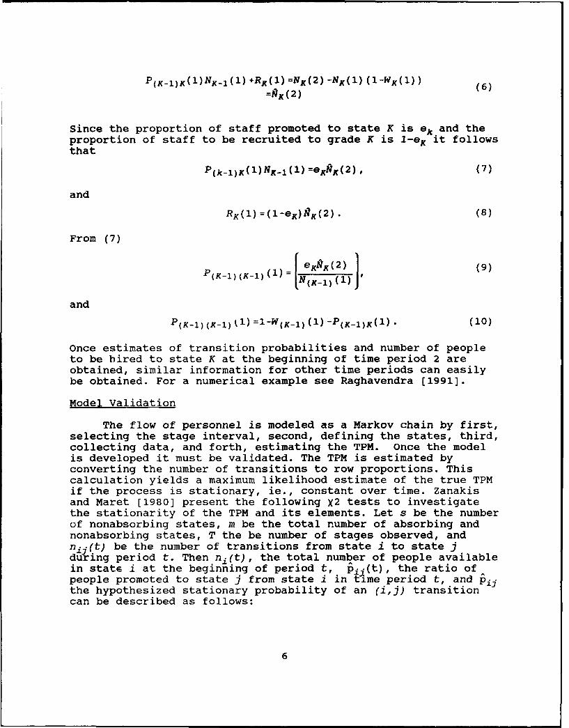
Once estimates of transition probabilities and number of peopleto be hired to state K at the beginning of time period 2 areobtained, similar information for other time periods can easilybe obtained. For a numerical example see Raghavendra [1991].

Model Validation

The flow of personnel is modeled as a Markov chain by first,selecting the stage interval, second, defining the states, third,collecting data, and forth, estimating the TPM. Once the modelis developed it must be validated. The TPM is estimated byconverting the number of transitions to row proportions. Thiscalculation yields a maximum likelihood estimate of the true TPMif the process is stationary, ie., constant over time. Zanakisand Maret [1980] present the following X2 tests to investigatethe stationarity of the TPM and its elements. Let s be the numberof nonabsorbing states, m be the total number of absorbing andnonabsorbing states, T the be number of stages observed, andnij(t) be the number of transitions from state i to state jduring period t. Then nh(t), the total number of people availablein state i at the beginning of period t, pi (t), the ratio ofpeople promoted to state j from state i in time period t, and pi.the hypothesized stationary probability of an (i,j) transitioncan be described as follows:

6

mni (t) Z-1 nij Mt (i

Pij (t) =nij (t) /ni (t) (12)

T T mPij= E nij (t)/ •nij t) (13)

t=1 t=1j =1

The following X2 tests may be used to test the stationarity ofthe TPM and its elements at the a level of significance.

(1) The (i,j) transition probability is constant over time if

TE ni(t) [pij-pij(t) ]2/pij < Xa 2[T-1). (14)

t=1

(2) Transitions to a column state j are stationary if

s TE ni(t) [(Pii pj(t) ] 21/pij < Xa2 [s(T-1)). (15)

(3) Transitions from a row state are stationary if

m T

E hi,(t) [Pij-Pij(t) ]2 /Pij < Xa2 [ (Mr-1) (T-i)]. (16)j=1 t=1

(4) The entire TPM is constant over time if

S m TE E E ni(t) [pij-_pij (t) ] 2/lpij < Xa2[CS (M-l1) (T-I1) ]. (17)

i=1 j=1 t=1

Markov models are used to obtain policies to achieve aspecific goal (structure of personnel) with no consideration forthe cost, possible constraints, or conflicting objectives. In the

7

following section the goal programming approach along with three

models developed for US Army and the US Navy are presented.

Linear Goal Proctramminc

Manpower planning can be formulated as a lineargoal-programming model, where each goal to be attained isrepresented by one constraint. The model objective is to obtaina compromising solution that will satisfy all the goals as closeas possible, when the exact attainment of all the goalssimultaneously is impossible.

Let xj denote the value of the jth Hacision variable. Let Gidenote the ith goal. Let I denote the number of goals to beachieved, and J denote the number of decision variables. Let a..denote the per unit contribution of the jth decision variableinto Voal i. Let gi denote the goal under-achievement variables,and gi denote the goal over-achievement variables; gI and gt arecalled deviation variables. Let wy and wj represent the priorityweights of under- and over-achievement of goal i. Therefore, ageneral formulation of the goal-programming model can berepresented as follows:

I I

Minimize Wt gt + • w- g- (18)i~l ai=1

J

s.t. • aij xj + gi - g. = Gi; i=l,...,m, (19)j=1

+ -+(20)+ i, g 2 o)

The determination of these priority weights is presented in thenext section.

Many manpower planning problems can be formulated as largegoal programs with hundreds of constraints representing thetargets and limitations. Several practical models have beendeveloped for these problems, such as the ASCAR and theELIM-COMPLIP models. These models and a Navy model are presentedin the following sections.

A US Navy Model

The manpower requirement for the US Navy is embodied in thepresent and future needs for a wide mix of specialties, withdifferent years of commissioned service. The US Navy has several

8

commissioning sources that have different capacities and costs.Some sources, such as the US Navy Academy (USNA), provideofficers with wide specialty areas, while others produce officerswith a single specialty. Therefore, to meet the future needs ofexperienced officers with different specialties, a proper mix ofthe commissioning sources must be established. A flexibleapproach is needed to provide a fast response to major changes inmanpower policies, and to study different scenarios of source mixand inventory costs.

The Approach. In this model, officer inventory within eachcommunity is specified by the number needed in different statesat each time period. An officer state is determined by threefactors: (1) warfare community, (2) commissioning program, and(3) years of commissioned service (YCS). Since most communitiesfollow a common promotion path in promoting their officers atknown YCS experience levels, YCS is then used as a substitute forgrades.

The expected flows between states in successive time periodsis projected, in a markovian trend, using transition ratesestimated from historical data. New accessions are also added tothese flows.

Formulation. The model developed by Bres, Burns, Charnes,and Cooper [1980] utilizes discrete time periods. The subscriptsused in this model are defined as follows:

i = Warfare community,j = Commissioning source,t = Time period,k = Number of years of commissioned service, andm = level of experience which is defined by lower and upperlimits on YCS.

The constants used in this model are defined as follows:

I = Number of communities,J = Number of commissioning sources,K = Maximum length of service,M = Number of experience levels,T = The planning time horizon,I-.(k) = Initial officer inventory in community i, form source j,wiih k YCS,Sý-(k) = Officer survival rate for t time periods in community i,from source j, with k YCS,Gim(t) = officers strength goal in community i, for experiencelevel m, in time period t,U(t) = Upper limit on total officer inventory in period t,B(t) = Budget limit for pay and allowances in period t,Cijk(t) = Cost for pay and allowances for an officer in communityi, from source j, with k YCS, in time period t,

9

I~m = Lower limit for YCS in experience level m for community i,ul, = Upper limit for YCS in experience level m for community i,X(t) = Upper limit on the total number of officers that may becommissioned in time period t,Pj(t) - Maximum number of officers that can be commissioned fromsource j in time period t,Qj(t) - Minimum number of officers that can be commissioned fromsource j in time period t,Ri(t) - Maximum number of newly commissioned officers that can betrained in community i, in time period t,Pij(t) = Maximum allowable number of officers commissioned fromsource j to community i, for time period t,Qij(t) = Minimum allowable number of officers commissioned fromsource j to community i, for time period t,wt (t) = Weight given to over-achievement of officer strengthgoal for community i, experience level m, time period t,wjm(t) = Weight given to under-achievement of officer strengthgoal for community i, experience level m, time period t, andw (t) - Weight given to negative deviation from total officerstrength limit, time period t.

The decision variables used in this model are defined as follows:

Yi.k(t) = Officers inventory in community i, from source j, withk CS, at the beginning of time period t.xij(t) = Accessions to community i from source j in time periodt.gýjm(t) = Goal under-achievement for community i, experience levelm in time period t.gi (t) = Goal over-achievement for community i, experience levelm, in time period t.g-(t) = Negative deviation from the total officer inventory upperlimit in period t.

The constraints that define the relation between officerinventories and goals, for each community at different experiencelevels, are expressed as:

J UimS•Yijk M)+ gira M)- g1M(t)= Gim~t M (21)

j=1 k=lim

where inventories can be expressed in terms of beginninginventories as:

Yijk(t)= Si (k-t)I9(k-t) for 2•t:k, (22)

and in terms of subsequent accessions as:The limitation on total officer inventories is expressed by:

10

Yijk(t) = Si (0) xij (t-k) for t>k. (23)

I J K

i • • Yijk(t)+ gj•1 (t)= U(t) forall t. (24).L1J=1 k=1

The budget limits are expressed by:I J KE E , Cijk(t)Yijk(t) M B(t) V t. (25)i=1 j=1 k=1

Restrictions on the officer accessions from various warfarecommunities are addressed in several constraints. The limitationon the total number of the officer accessions in each period isexpressed by:

I Jx x13 (t) • P(t) V t. (26)

i=1 j=1

In each community, the training capacity limits for newlycommissioned officers are expressed by:

J

Sxij(t) • Ri(t) V i, t. (27)j=1

The operating upper and lower limits for the commissioningsources are expressed by:

IQj(t) M : xij(t) • Pj(t) V i,t. (28)

i=1

The upper and lower limits on the distribution of newlycommissioned officers from each source to each community areexpressed by:

Qij(t) M xij(t) 5 Pij(t) V t. (29)

Let o(t), P(t), 7f(t), and S(t) denote the minimal and maximalproportions of change allowed between adjacent time periods. Theproportional changes allowed for inputs to each community areexpressed as follows:for the accessions to community i. The proportional changesallowed for outputs from each source are expressed as follows:for the output of source j. Finally, a nonnegativity condition isimposed.

11

J J Ja (t) T1 x1 3 (t) :5 T' X1 3 (t+l1) -. 0(t M x1 3 (t) V t and (30)

-7 1 71 j

I I I

I(t)• M i Xij(t) i E x1ij(t+l) 5 6(t) f xij(t) V t and (31)i=1 i=1 1=1

The model objective is to find an officer accession and anarrangement plan that minimizes weighted deviations from officerstrength goals. This can be expressed as follows:

T I M T

Minimize E E E (w+(t)g+(t)+w,.(t)g - (t)) +• w-(t)g-(t),t=1 i=1 m=1 t-1 (32)

subject to constraints (21)-(31).

As an illustration, the model was applied to fourcommunities (Unrestricted Line officers) for the first ten yearsof commissioned service omitting the budget constraint. Itprovided a satisfactory accession plan with minimal deviationsfor the high priority requirements. For more details see Bres,Burns, Charnes and Cooper [1980]. The model can also be used toprovide the impact on budgets if the appropriate results aresubstituted into constraint (25) to study funds-flow consequencesof these plans.

The ASCAR Model

The Accession Supply Costing and Requirement (ASCAR) modelis a goal programming based model. It was initially developed byGeneral Electric for the Congressional Budget office in the lateseventies. The model was then revised and used by the office ofthe Assistant Secretary of Defense. The main objective of theASCAR project was to provide the capability to investigate theeffects of changing manpower policies on personnel requirements,tiilitary qualifications, and the associated costs.

The ASCAR model consists of data management programs, a database, personnel flow simulation routines, a cost routine, and areport routine. It follows a five-step process to evaluate theannual accessions necessary to meet the strength and qualityrequirements, and to calculate the associated costs. These stepsare summarized in the following:

* Initially, the historical data are analyzed to developflow rates and starting personnel levels for the simulatedperiod.

12

9 These rates and levels are then used in the personnel flowsimulation routines to compute losses, to forecast thesupply of new recruits for each simulated year, and tosimulate the flow of new recruits in order to calculate therequired accessions.

* The supply of new recruits is categorized by sixtyqualitative factors such as educational level and mentalcategory.

* The goal programming procedure optimizes the differentcategory mix of new recruits to match the requiredman-strength and characteristics while satisfying thespecified constraints.

* The cost module produces the cost estimates for theanalyzed policy using the cost factors and the projectedstrength determined in the previous steps.

The process is then repeated for each additional year. More

details are provided in Collins, Gass, and Rosendahl [1983].

The ELIM-COMPLIP Model

The Enlisted Loss Inventory Model-Computation of ManpowerPrograms Using Linear Programming (ELIM-COMPLIP) is a goalprogramming based forecasting system developed by GeneralResearch Corporation for the Department of the Army. It is usedfor manpower planning, budgeting, and personnel policyformulation. The system is described in details by Holz [1980].

In the late sixties the Assistant Secretary of the Army,William K. Brehm, was addressing several "what if" questionsrelated to different manpower policies for Vietnam. Eachalternative required approximately 8-20 computation hours.Therefore, the General Research Corporation was asked to automatethese computations. One of the two systems developed was theCOMPLIP optimization system. The main objective of COMPLIP is tominimize the weighted sum of the deviations of the actualman-strength from the required goals. It provided the fastresponsiveness needed to generate accurate manning plans formodels with conflicting constraints that were difficult toapproximate by manual calculations. The second was a simulationof the manual system. It '-as never used after the demonstrationof the COMPLIP system. COMPLIP provided upper and lower bounds ondraft calls that were very useful in preventing fluctuations tothis sensitive political issue.

In the fiscal year 1972, the Army was phasing down fromVietnam, when the Congress passed an authorization bill to reducethe Army's strength by 50,000 for that yea-, which significantlyaccelerated the phase-down plan. Several drastic policies were

13

adopted that disrupted personnel management and caused thestrength to fall below authorized level. The Army ended the year50,000 men below the desired strength. As a response to thiscrisis, the General Research Corporation developed the EnlistedLoss Inventory Model (ELIM) using a new loss projection method.The new method starts with the most recent information andpreserves the relations between end strength, gains, and lossesto avoid the risks created with the previously used process.

The ELIM-COMPLIP system is self-correcting with respect toprojection errors, and provides accurate strength forecasts. Itincludes five modules: data processor, rate generator, inventoryprojection, optimization, and a report generator module. Theprimary task of the rate generator is to exponentially smooth thetime series of historical data to project loss rates. These ratesare used in the inventory projection module to compute retentionrates that develop the goal programming coefficients. For moredetails see the description and the system schematic in Holz[1980].

Goal Weight Evaluation

Linear goal-programming has proved to be very effective insolving multi-criteria problems, such as manpower planningproblems. Usually, the objective function (18) of a generallinear goal-programming model (18)-(20) contains severalthousands of deviation variables. Most problems have specificproperties that necessitate proper determination of weights, wiand wi, associated with the deviation variables to reflect thecorrect goal priority. In general, direct weight determinationfor small problems with related goals is not a hard task.However, direct weight determination for thousands of dissimilargoals is not viable, as it resembles comparing "oranges toapples". In this section we represent a weight determinationapproach proposed by Gass [1986) using Saaty's analyticalhierarchy process (AHP).

Consider the grade-skill goal constraints (21), budgetconstraints (25), and promotion goal constraints (30). Meetingany of these constraints has a completely different meaning thanmeeting the other two. Also, meeting a grade-skill goal in oneyear may have a much different priority than the same goal in adifferent year. Therefore, planners must be able to designate theobjective goal weights that cause a proper transition to be madeover the planning horizon to reach specified requirements atcertain years. Undoubtedly, the exact matching of man-strengthrequirements that fluctuate over the intended period is notachievable. However, a compromising solution can be accomplishedwhere the goal weights will determine the years to be closelymatched, namely, the solution profile.

14

Gass [19861 developed an automated routine for calculatingthousands of weights necessary to determine an acceptablesolution for the linear goal program (18)-(20).

A grade-skill model with a seven year planning horizon is" sed to illustrate Gass' method. In this model the goals aredefined by (1) total personnel at the end of each year, (2)grade-skill qualifications, (3) promotion goals by grade-skill,and (4) loss goals by grade-skill. These goals can be representedby a hierarchical structure of factors illustrated in Figure(l).Level 1 represents the model main objective. Level 2 contains themajor requirements (year end-strength) that influence the model.Level 3 contains the grade-skill, promotion, loss, and gaintargets that influence level 2.

Level 1 Army personnel program

Total end-

Level 2 strength Year 2 Year 3 Year 4 YearS5 Year 6 Year 7Year 1

Level 3 Goal - skill Promotion Loss Game

I targets targets targetstags

Figure 1. A hierarchy for personnel goal priorities (Gass,1986)

The Gass method establishes the overall priorities in themain objective from the hierarchical factor priorities bysystematically comparing the factors within each level. In eachlevel, the weights that reflect the factor priorities areobtained from a comparison matrix associated with the level. Thematrix elements have values 1 to 9 and their reciprocals, andrepresent the importance of meeting each factor. A typicalcomparison matrix corresponding to level 2 of the above exampleis:

15

15 3 1 3 3 31/5 1 1/5 1/3 1/5 1/7 1/9A /3 5 1 7 7 9 91 3 1/7 1 3 5 7

/3 7 1/9 1/5 1/3 1 5

/3 9 1/9 1/7 1/3 1/5 1

where A1, 4 =1 means that year 1 and year 4 are equally important,and A7 2 ý=9 means that year 7 is significantly more important thanyear 2, with respect to the model main objective. The Gass methoddetermines the solution to the system of equations Aw= Aw, whichis the well-known eigenvalue problem. Following the AHP theory,for X equal to the largest eigenvalue, the normalized wicomponents are then interpreted as weights that represent theimportance of each factor. For the above matrix we have thefollowing weights for level 2:

Year 1 2 3 4 5 6 7Weights 0.25 0.03 0.38 0.18 0.07 0.08 0.01

These weights indicate that the accomplishment of year 3's goalhas the highest priority (0.38), then year l's goal and so on.

A similar analysis is carried out to determine the level 3factor priorities for each year. The composite goal prioritiesfor the level 3 items are developed by multiplying the year'spriorities by the corresponding factor priority, and then adding.A detailed example is described in Gass [19863.

Finally, the AHP priorities are converted to goal weightsfor each target-year combination. This is accomplished usingcloseness factors. Each target-year combination is characterizedby an ordered couple c(i,j), in this example i=i,...,4 (targets)and j=l,...,7 (years), which adjusts the composite weight fortarget i to account for the priority of year j. Thus, weight forany goal i and year j is determined by

16

W, = i CU ) 5(33)5

where SP is the top of the scale for goal i and Sý is the bottomof the scale for target i. A broad scale (e.g. 0 to 1000) is usedso that the optimization algorithm would be able to differentiateproperly between the goals.

The AHP theory can be extended to determine the skillweights for each grade, in order to set priorities between theskills within a grade for each year. An example of weightsindexed by grade and skill is given in Gass [1986].

Markovian Goal ProQramming

Even though Markov models are successfully used to estimatethe future manpower plan or to develop policies to obtain adesired future personnel structure, they cannot consider cost,constraints, or conflicting objectives. Zanakis and Maret [1981]use a combination of the Markovian and LGP techniques to obtain amanpower plan. As previously stated they use historical data toestimate TPM and desired structure of the personnel system. Oncethe number of personnel is determined they develop a goalprogramming model to satisfy the organizational goals such as:keep the cost at the lowest possible level, hire a specificnumber of recent college graduates, keep the ratio of number ofpersonnel at a specific level of employment to other levelsconstant, and other similar goals. For details and a numericalexample see Zanakis and Maret [1981].

Assuming that costs can be assigned to under and overproduction and given the time demand level will reach steadystate, Young and Abodunde [1979] present a formulation for adiscrete-time Markovian goal programming model.

Let G(t) denote the target demand at time period t, andC-(t) and C+(t) denote the costs ascribed to the goal under- andover-achievement. Let R(t) denote the total recruit inventory attime period t, and Ys the number of units surviving the first syears of service. Let P denote the transition probability matrix,•0 denote the recruitment vector, and (1-a) denote the failurerate. Then, the linear goal programming model (18)-(20) can bestated as follows:

T

Minimize E ( C(t)g÷(t) + C-(t)g(t) ) (34)C-1

17

t

s.t. E Ys Rt: 1 -8 + g-(t)- g+(t) = G(t); t=l,...,T, (35)s=1

Ys= { pS-1 + tp9-2 + + as-ll }go. (36)

Notice the resemblance of (35) and (36) to (21) and (22).

Other constraints such as limits on the number of recruitsfor some or all of the periods under study can be added. Thetechnique is applied to a case study based on the Irish TelephoneSystem. Numerical results are presented in Young and Abodunde[1979).

Conclusions

Markov models are valuable tools in manpower planning.Stochastic and deterministic models are developed andsuccessfully used to predict future manpower structures, toderive policies to achieve a specific manpower structure in thenear and far future, and to provide insight to "what if'questions. Historical data are used to estimate the TPM. Theestimated TPM is not very accurate, so the results from Markovmodels must be used cautiously. Deterministic models arepreferred by some practitioners since they believe that forecastsare not accurate enough to justify the complexity of thestochastic models. Even though, Markov models are very helpful inmanpower planning they do not take into account costs orconflicting objectives.

Manpower planning is closely linked to linear programmingtheory. Manpower planning problems can be represented as a lineargoal-programs, where limitations and conflicting goals areformulated as constraints with objectives to minimize thedeviations from these limitations. Several practical models haveused this approach for solving manpower problems. This approachhas proven to be very efficient in providing satisfactoryresults. In goal programming model, goal priorities have asignificant role in determining how closely each goal is matched,and consequently, the solution profile. One of the suggestedtechniques for determining the objective weights, that reflectthe priorities, is to systematically compare the main factors atdifferent levels of the problem. Most of the data used in thesegoal programs rest on assumptions and predictions about severalhuman and economic factors, e.g. officer survival rate. Toproperly incorporate these nondeterministic factors, Markovmodels are used to quantify these predictions to be used asgoal-program constants.

18

The Prototype Model

The model described below is designed so that two reportscan be generated and used for decision making. The inputs to themodel are the following:

(i) the force structure,(ii) inventory targets,(iii) promotion targets, and(iv) transition rules for personnel who move through the system.The output tables take the following form:

Personnel Inventory Report

Time Grade Policy Target Inventory Deviation %Group (Input) Produced Deviation

By TheModel

Personnel Promotion Report

Time Grade Target % promoted % Promotionsat this produced by

(Time,Grade) thecombination model

(input)

19

Graphical Display

35

30

25 -

20

10

5

12 3

Yýr

E2Targat Mode I O"Ut~u

Figure 2. Inventory target and model output for grade g andpolicy group i

Subscripts

t- denotes the time period (years)g- denotes the grader- denotes the location (r=l conUS, r=2 not conUS)i- denotes a policy groupm- denotes the number of years in policy group iIt is assumed that all personnel can be characterized by a 5-tuple given by the 5 subscripts. We will refer to a 5-tuple(t,g,r,i,m) as a state from which a transition can be made toanother state.

20

Graphically this may be viewed as follows:

AA A(At g, r, i, m+

SEP '•/•"

..... " r, "r rn=m

(t~gtr~ir) - stat

A A

ACC~~~~~ ~~~ -A reo e t e o i i n de f r a l Acc s i n

tg, r, i+1, 1A

SEP }if M=t,g+1, r, i+1,I Z

The rules for the possible transitions are input to the model.

Node Names

(t,g,r,i,m) - stateACC - denotes the origin node for all accessionsSEP - denotes a destination node for all separationsBAL - denotes a balance node to balance the supply anddemand in the model. This is required for a true network model ofthe form AX=r where A is a node-arc incidence matrix.

Arc Types

(t~~r~~m~~l~,~i~fi)- arcs which corresponding to moving fromstate (t,g,r,i,m) to state(t1,?if)(ACC;t,l,r,1,l) arc from the node ACC to state (t,1,r,l,l).(t,g,r,i,m;SEP) arc from the node (t,g,r,i,m) to the separationnode.(H,g,r,i,m;BAL) arc from state (H,g,r,i,m) to the node BAL.(SEP;BAL) arc from node SEP to node BAL.

21

Startingsupply}

1,1

• SEPi I {Ending:t'"" gr..mdearnd

BA

SSEP

.,g. r, i. m.

:SEP

t=1 t=H

Figure 3. General structure

22

05

.. .. .. ..

EE

*< E

LU uIIU

C4l)

< 4-b

V)-$4

00

23

Constants and Sets

H- planning horizon (t=1,...,H)T(gr,i,m) - the set of nodes ( for which there exists anarc (t,g,r,i,m;t+l,gri,•) for t=l,...,H-1. This is sometimescalled the to set or the after set.F(g,r,i,m) - the set of nodes (t-l,•,Ft,•) for which thereexists an arc (t-l,grii;t,g,r,i,m) for t=2,...,H. This issometimes called the from set or the before set.RHS(g,r,i,m) - number of people in the state (1,g,r,i,m)ES(t,g) - force structure (people)N(t,g,i) - inventory targets (people)PROM(t,g) - Promotion Targets (%)W1, W2, W 3, W 4 - weights for deviations from targets.

Decision Variables

X(t,g,r,im;t+l,g,r,!,m) - number of people on the arc(t,g,r,i,m;t+l,,-rofo)I(t,g,i) - number of people who leave state (t,g,i)P(t,g) - number of people who leave state (t,g) and are promotedA(t,r,1,1) - number of people on arc (ACC,t,l,r,l,1)B(g,r,i,m) - number of people on arc (Hg,r,i,m;BAL)C - number of people on arc (BAL,ACC)D - number of people on arc (SEP,BAL)S(t,g,r,i,m) - number of people on arc (t,g,i,m;SEP)IO(t,g,i) - number of people over the desired inventory levelIU(t,g,i) - number of people under the desired inventory levelPO(t,g) - number of people over the desired promotion % goalPU(t,g) - number of people under the desired promotion % goal

24

Constraints

Conservation of Flow (t.c.i~m)=(l.l. I)

EX(1,1, r,1, 1; 2,ý, 7, -,mT) - S (1, 1, r,1, 1) A A(1, r,11(j.7,T,.5 eT(2, r. I.m)

- RHS(1,.r, 1 1) V (r,i,m)

40

ACC0/

1 RHS(I~r.I,I) •"......

1, ~2 2,r 1, - 2....

. SEP2, 1, 2, I,

22,. }ifM=l

-...... ....

Figure 5. Conservation of flow t=1, g=l

25

S

Conservation of Flow t=l, (g,i,m)q#(l,l,l)

SX(l,g,r,i,m;2,5,T,,T, 7f) + S(l,g,r,i,m)(7,T T) e T(g, r, 1,m)

RHS(g,r,i,m) V (g>l,r,i,m)

•g~rgm r,m

FigureSE 2. Cosrvto offoi~, g+1

26 r, i, m+1

A A2, g, r, i+l, I '

.A.A if mn =M

Figure 6. Conservation of flow t=l, g>1

26

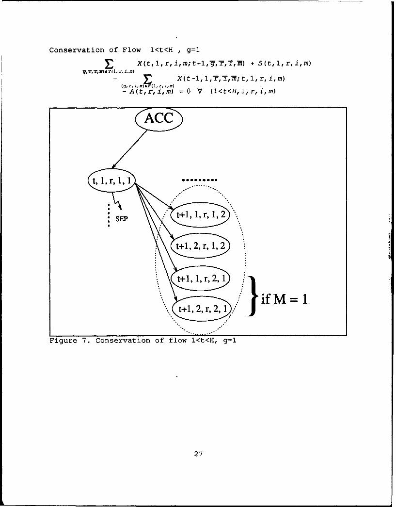
Conservation of Flow 1<t<H , g=l

X(t,1,r,i,m;t+1",T,,T, M) + S(t,l,r,i,m)

- X(t-l, 1,7,T,M; t, 1, r, i, m)(g, r, Im)EF(1, r, I,m)

A(t,r,i,m) = 0 V (l<t<H,l,r,i,m)

ACC

l~tr, 1, r, -------

M M

t+1, 2, 2, 1,

Figure 7. Conservation of flow l<t<H, g=l

27

Conservation of Flow 1<t<H, (~~n#lll

IE X(t,g,r,j,m;t+l,Th?,T,7177f) + S(t,1,r,i,m)

- X~-1,~7,T~; t gr, im) 0 V (l<t<H,g,.r,i,m)

t-,g, r, i, m

SEA A A

g,1, r, m+

1I,g+1,r,i,m+l

t+1,g+,r,i+1,1

Figure 8. Conservation of flow 1<t<H, (g,i,m)#(1,l,1)

28

Conservation of Flow t=H, (g,i,m)=(1,1,1)S (H,1, r,I1,1) +B (1,r,1,1) - A (H, r,1,1) =0

Figure 9. Conservation of flow t=H, (gi,m)=(l,1,1)

29

Conservation of Flow t=H, (g,i,m)i#(l,l,l)

S (H, g, r, i, m) - E X(H-l, ,-fT,;ff,;Hg, r, i, m)(TrT,N7 EF(g, r, I,,,)

+ B(g,r,i,m) = 0, V (g,r,i,m)

BBAL

,g+I,r, 1, n+1

H, g, r,i+1,1Iif M=M

H, g--, r, i+I,1

SEPFigure 10. Conservation of flow t=H, (g,i,m)•d(l,l,l)

~30

.,. }

Conservation of Flow at ACC

SA(t,r,i,m) - C = 0( r, i, m)

SEP SEP

Figure 11. Conservation of flow at ACC

31

Conservation of Flow at SEP

D S ~ (t, g, r,j,m) = 0

Inventory Constraints t<H

+E S(t, g, r, i, )-IQ, g, i) =0, Al t<H, g, i)

t, g, r ,j SEPI

SEP

Figure 12. Inventory constraints t<H

32

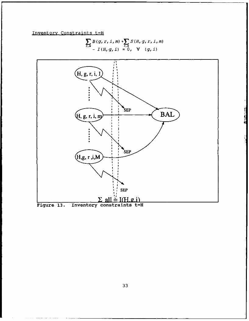
Inventory Constraints t=H

E B(g, r, i,m) +ES(H,g r,i,M)Il(H, g, i) = , (g, i)

SE

SEP

Figure 13. Inventory constraints t=H

33

Force Structure Constraints

F I(t,g,i) = ES(t,g) , V (t,g)

Promotion Accounting Constraints t<H,g<GS• X(t, g, r, i, m; t+1, g+l,-f,T,7f)

- P(t,g) = 0 V (t<H,g<G)

o. ..... °...

* t+1Ig,r~i+1, I I

if m= M

X all - total promotionsFigure 14. Promotion accounting constraints t<H, g<G

34

Deviation From Inventory GoalI (t, g, i) + XU (t, g, i) - IO (t, g, i) = N (t, g, i), V (t, g, i)

Deviation From Promotion Goal

P(t,g) + PU(t,g) - PO(t,g) = PROM (t,g)ES (t,g), V (t<H,g)

Objective Function

minimize (W1IU(t,g,i) + W210(t,g,i))(t,g,i)

+ E (W3 PU(t,g) + W4 PO(t,g))(tg)

Constraint Layout

Name Size

States ST H.G.R.I.Mt,gr,i,m

ACC ACC 1

SEP SEP 1

BAL BAL 1

Inventory INV H.G.I

Force FOR H.G

Promotion PRO (H-1).(G-1)

Inventory Goal IG H.G.I

Promotion Goal PG (H-1). (G-1)

Total Constraints = H.G.R.I.M + 2.H.G.I + 2.(H-1).(G-l)+ H.G + 3

35

Column Layout

Row Name Column Name SpecialCondition

X(t,g,r,i,m;t+l,g,qr,,I) t<H

ST(t,g,r,i,m) 1ST (t+ 1, g,r, 1,m) - 1i_ _ __ _ _ _

INV(t,g,i) 1PRO (t, g) 1 if•>g

Row Name Column Name Special Condition

I(t,g,i)

INV(t,g,i) -i

FOR(t,g) 1

IG(t,g,i) 1

Row Name Column Name Special Condition

P(t,g) t<H

PRO(t,g) -1

PG(t,g) 1

Row Name Column Name Special Condition

A(t,r,i,m)

ACC 1

ST(t,l,r,i,m) -1

Row Name Column Name Special Condition

B(g,r,i,m)

BAL -1

ST(H,g,r,i,m) 1

INV(H,g,i) 1

36

Row Name Column Name Special Condition

CBAL 1

ACC -1

Row Name Column Name Special Condition

D

SEP 1BAL -1

Row Name Column Name Special Condition

S(t,g, r, i,m)

SEP -1

ST(t,g,r, i,m) 1

INV(t,g, i) 1

Row Name Column Name Special Condition

IO(t,g, i)

IG(t,g,i) -1

OBJ W2

Row Name Column Name Special Condition

IU(t,g, i)

IG(tg,i) 1

OBJ W1

Row Name Column Name Special Condition

Po (t, g)

PG(t,g) -1

OBJ W4

Row Name Column Name Special Condition

PU(t, g)

PG(t,g,i) 1

OBJ W3

37

References

Abodunde, T., and S. McClean, 1980, 'Production Planning for aManpower System with a Constant Level of Recruitment,' AppliedStatistics, Vol. 29, No.1, 43-49.

Bartholomew, D., 1982, Stochastic Models for Social Processes,John Wiley and Sons, New York, New York.

Bres, E., D. Burns, A. Charnes, and W. Cooper, 1980, 'A GoalProgramming Model For Planning Officer Accessions,' ManagementScience, Vol. 26, No. 8, 773-783.

Collins, R., S. Gass and E. Rosendahl, 1983, 'The ASCAR Model forEvaluating Military Manpower Policy,' Interfaces, Vol. 13, No.3, 44-53.

Edwards J., 1983, 'A Survey of Manpower Planning Models and TheirApplications,' Journal of Operational Research Society, Vol.37, No. 11, 1031-1040.

Gass, S., 1986, 'A Process for Determining priorities and Weightsfor Large-Scale Linear Goal Programmers,' Journal ofOperational Research, Vol. 37, No. 8, 779-785.

Hall, R. W., 1986, 'Graphical Models for Manpower Planning,'International Journal of Production Research, Vol. 24, No. 5,1267-1282.

Holz, B. and J. Worth, 1980, 'Improving Strength Forecasts:Support For Army Manpower Management,' Interfaces, Vol. 10, No.6, 37-52.

Smith, A., and Bartholomew, D., 1988, 'Manpower Planning in theUnited Kingdom: An Historical Review,' Journal of OperationalResearch Society, Vol. 39, No. 3, 235-284.

Raghavendra, B., 1991, 'A Bivariate Model for Markov ManpowerPlanning Systems,' Journal of Operational Research Society,Vol. 42, No. 7, 565-570.

Vassiliou P., 1976, 'A Markov Chain Model for Wastage in ManpowerSystems,' Operational Research Quarterly, Vol. 27, No. 1,57-70.

Vajda, S., 1976, Mathematics of manpower Planning, John Wiley NewYork.

Young, A. and T. Abodunde, 1979, 'Personnel Recruitment Policiesand Long-term Production Planning,' Journal of OperationalResearch Society, Vol. 30, No. 3, 225-236.

39

Zanakis S. and M. Maret, 1980, NA Markov Chain Application toManpower Supply Planning," Journal of Operational ResearchSociety, Vol. 31, No. 12, 1095-1102.

Zanakis S. and M. Maret, 1981, "A Markovian Goal ProgrammingApproach to Aggregate Manpower Planning,' Journal ofOperational Research Society, Vol. 32, No. 1, 55-63.

40

Appendix AModel Generator and Test Case

A-I

Z b

u u uo o

.w 000. Z

T T

0 w.

i56600 1-0 - 1

- .P .2 a

4020u- .. U

KUW0. c. 0a.

0 .. - 0

* - - . . J ~ .I 0* 5

- .06U S - - -- U~a KoaS -.

a a U Z a a. . -

.*3 C... .. .. ... .. .. ..

0

Kc

I S S

o

o

CLC

-0 0.-

2I a

00

-- 0S. o

UU c

-C

u A -

-~~4 zc -8--

II-

ig 1i

0. 0.- 0.0..Ct

.......... "

S -V

IL

U- U

Un- U w :V o uuo0

C-6

ii9

U A OA - a

v ~ ~ ~ ~ U S-UU 6 00 IU uco~ cc-

9-V

16 -1 .4

lea 1. -u

E E

33 ZS - o o -

I 0 e

we .*3 5 -

L -V

EE

* * E

.cA cc - 3 . .

c e- --- -U - -

I = -. iC ===H i E E .. 1 -*-S- E E -t '0. 'olS4UOO

E E

At u-. 19 C U

E. 1. 122 1 m

o E *** *** :u 00 84 *t I* 4U

8-V

'1 1 IU I _

EE

, !! •,• ... ,...

El I;

i..2ii

HISC of u

.-."-."- i - ii t

V A0

E EEE . ' -- E E E ..

|. . o - =o- . o ' !•= li,-

""00 00 - o CA

ILi . .. ... . ...

S......... .o$::•:•..1

2 ,o ,I, ,

6-V

JA

"aIC! to"-12- .

-- -- .U

- N - -u --

C2 t 0 a-

, 12 . .•St .- - am

e. - s a6 C si; t: O ni

So -0 zi- i *

a~ A.. a I I t* U A. A - U

.0 --. U

0 0

aa1 cc

8,6 6 sz

25 g u. 4 =E4

S.s S1 g == 3 21 S !=-l l

so C- 4 . 0 "C -. C- .5 U4 .4.* 02

--Lu

B: t e.2 t 8 :

* as . 5 4 -. ~S u u a.~V 0 54 ~

ug ~ ~ ~ &MO

0.9

A'~~~ ~ "r' 0sl

0~~~~ 0 lx U 0 u0

TT-

r 0 42'oA c

13 8 1i u 011= :u 2 -4. 3U 42 -211U o c 4 1 1

~~~-~ - c- ~3 -go 0 -c CA -C '

*020

u E u~ 6 v u E I uuv

u ~ IU 2v- u . vu u c

u~ u

LA~

T-fV

OU r

ou :U! 00

U4 8 2

asa

V Am

c c 4,CU* U - . u c - -O

ST -V

*p 0

I a.m to

a tt g I'66 66C

141 I2 u Z Z v- .0

.C a

a. 16ga . - -

- 6 i~ *-~ -- -

2 -~ 6* .6 -~ i At*~~~~ Mal6 3 - * - -

.it U -

i� T -v

I-0

Ii-

2

SM MM

'! !' '!n� *W �a --** ** SO @0

-M atM SM MM

! H H�e cc �c

- 0 --

h� MM MM 1 MM00 00 00 0 00

MM at MM

3 3 3 3'C-

I. � j� :�__ �. a. *�

.[U

S *i i -i N