The Application of Hybrid Evolving Connectionist Systems to Image ...

The Application of Hybrid Evolving

Connectionist Systems to Image Classification

Nikola K. Kasabov#

Steven A. Israel*

Brendon J. Woodford#

University of Otago

#Department of Information Science

*Department of Surveying

PO Box 56

Dunedin

NEW ZEALAND

This paper presents a methodology for image classification of both spatial and spectral data with

the use of hybrid evolving fuzzy neural networks ( EFuNNS). EFuNNs are five layer sparsely co n-

nected networks. EFuNNs contain dynamic structures that evolve by growing and pruning of neu-

rons and connections. EFuNNS merge three supervised classification methods: connectionism,

fuzzy logic, and case-based reasoning. By merging these strategies, this new structure is capable of

learning and generalising from a small sample set of large attribute vectors as well as from large

sample sets and small feature vectors. Two case studies data are used to demonstrate the effectiv e-

ness of the methodology. First, an environmental remote sensing application, and second, large

scale images of fruit for automated grading. The proposed methodology provides fast and accurate

adaptive learning for image classification. It is also applicable for on-line, real-time learning and

classification.

Keywords: image classification, hybrid systems, neural-fuzzy systems, evolving fuzzy neural networks.

1. Introduction: Approaches to Pattern Recognition

Most image pattern recognition tasks usually involve six major sub-tasks: image segmentation, target

identification, attribute selection, sampling, discriminant function generation, and evaluation. This paper

focuses upon a novel approach for generating discriminant functions that overcome the limitations of

conventional algorithms. Specifically, this new approach is capable of processing high dimensional fea-

ture vectors, suitable for evaluating both static and dynamic input streams.

Perlovsky 33) defined three classes of pattern recognition algorithms based on how they divide the feature

space into acceptance regions: discriminating surfaces, nearest neighbours, and model based approaches.

Pattern recognition algorithms can also be viewed by how they apply knowledge in model based, rule

based, and example based approaches. Model based algorithms include all deterministic and probabilistic

algorithms where discriminant functions are generated by prior knowledge of the acceptance region’s

structure in the feature space. Many of these algorithms fall into Perlovsky’s definition of a nearest

neighbour algorithm. For these algorithms, few examples are required to estimate the number of pa-

rameters. Another advantage is that when data fits the assumed model, an estimate of the mapping preci-

sion can be determined prior to analysis. However, there are costs for model based algorithms. The data

must support the model and the entire population must be fully “visible”, available and representative.

Generally these algorithms are unadaptable.

Rule based algorithms apply expert knowledge. They divide the feature space by defining boundaries

between acceptance regions. Inferences are generated based upon the expert knowledge implemented in

the system. Rule based algorithms are usually not adaptable. However, mapping errors can be minimised

using tuning rules to adjust the acceptance regions – but the consequences are severe. Often the exact

mapping from the inputs to the outputs is unknown. The generation of rules requires a large amount of

direct operator invention. Because rules form discriminating surfaces, new rule sets are required when

the data distribution is not static, and output labels, or extracted attributes change.

The example based approach minimises the limitations of model based and rule based algorithms. Exam-

ple based algorithms do not contain any prior knowledge about the structure of the acceptance regions in

the feature space. Often they operate by building discriminating surfaces, making them adaptable. The

drawbacks are that they require a large number of training examples to estimate a large number of inde-

pendent parameters.

For complex image processing tasks the three models are limited by different resources. Model based

approaches are limited by the available computer space since all the examples must be fully “visible” to

the system prior to generating the discriminant functions. Rule based systems are limited by problem

complexity, and example based systems are limited by processing power.

In addition to the algorithmic structure, image pattern recognition algorithms are plagued by the dilemma

of discriminant function specification versus generalisation. In order to obtain a high degree of similarity,

discriminant functions must map the inputs to a small feature space distance to their known outputs. For

high precision, a high-order discriminant function is required. However, these high-order functions do

not generalise well to new data. These two exclusive criteria must be optimised.

One way to utilise the advantages and to overcome the disadvantages of the different methods above is to

merge them into one system. In Section 2, the characteristics that form the basis of EFuNNs are identified

and compared to conventional fuzzy neural networks. Section 3 and Section 4 highlight two case studies

for image classification. In the first case, a single image is used to map land cover types over a limited

area. The classification problem is defined by a large number of static data points having a small feature

vector. The second case is the operation of an image library to identify defects in fruit. This case is de-

fined by a limited dynamic set of images each containing a large number of attributes.

Advances to the image pattern recognition problem have occurred on several fronts. The most notable

were Zadeh’s idea of fuzzy membership functions 2,28,24,30,31,32,41) and the connectionist approach 5,25,26,27).

De-convolution of attributes from crisp values to membership degrees has been shown to increase the

ability of the discriminant functions to generalise and assign more precise labels 3,19). The connectionist

learning paradigm proved to be valuable for image classification too.

Perlovsky 33) cited that the argument between prior knowledge and adaptability has continued throughout

the history of science. Grossberg 5,9) defined this as the stability/plasticity dilemma. Optimum pattern

recognition algorithms were identified as requiring a mix of these seemingly exclusive properties. Al-

though no unifying mixture of algorithms has been identified, rules based algorithms have been success-

fully mixed. These hybrid systems include fuzzy neural networks and neuro-fuzzy systems, 10,12,14,15,16),

symbolic rule based algorithms mixed with neural networks 14), and example based algorithms 17-22), hy-

brid statistical methods 8,2,6,11) and hybrid evolutionary methods 7,39).

Example based algorithms can be broken down into two basic categories: (1) case based reasoning 13), and

(2) connectionist algorithms 8). Fundamentally, these two algorithms process data differently. For case

based reasoning, case examples (exemplars) are stored in memory. New examples are compared to ex-

isting cases based upon attribute similarity. The discriminant functions do not contain specific parameters

to estimate. With connectionist architectures, none of the individual examples are stored. For each class,

the similarity among the intraclass examples and the difference with the interclass training examples de-

fine the acceptance region. The former allows for dynamic adaptable training at the cost of huge memory

requirements, while the latter is noise tolerant and provides a smooth asymptotic relationship between

processing time and mapping precision.

2. Fuzzy Neural Networks (FuNN) and Evolving Fuzzy Neural Networks(EFuNN)

2.1. Fuzzy Neural Networks

Fuzzy neural networks are neural networks that realise a set of fuzzy rules and a fuzzy inference machine

in a connectionist way 3,4,12,14,15,16,30,34,35). We shall use this term to cover also all fuzzified connectionist

modules 3,4,10). FuNN is a fuzzy neural network introduced in 14) and developed as FuNN/2 in 16). It is a

connectionist feed-forward architecture with five layers of neurons and four layers of connections. The

first layer of neurons receives the input information. The second layer calculates the fuzzy membership

degrees to which the input values belong to predefined fuzzy membership functions, e.g. small, medium,

large. The third layer of neurons represents associations between the input and the output variables, fuzzy

rules. The fourth layer calculates the degrees to which output membership functions are matched by the

input data, and the fifth layer performs defuzzification and calculates exact values for the output vari-

ables. A FuNN has features of both a neural network and a fuzzy inference machine. A simple FuNN

structure is shown in Figure 1. The number of neurons in each of the layers can potentially change during

operation through growing or shrinking. The number of connections is also modifiable through learning

with forgetting, zeroing, pruning and other operations 14,16).

The membership functions (MF) used in FuNN to represent fuzzy values, are of triangular type, the cen-

tres of the triangles being attached as weights to the corresponding connections. The MF can be modified

through learning that involves changing the centres and the widths of the triangles.

Fig.I

Several training algorithms have been developed for FuNN 14,15) and several algorithms for rule extraction

from FuNNs have been developed and applied 14-16). One of them represents each rule node of a trained

FuNN as an IF-THEN fuzzy rule.

FuNNs are universal statistical and knowledge engineering tools 3,4). Many applications of FuNNs have

been developed and explored; such as pattern recognition and classification; dynamical systems identifi-

cation and control; modelling chaotic time series and extracting the underlying chaos rules, prediction and

decision making 14). A FuNN simulator is available as part of a hybrid software environment Fuzzy-

Cope/3. Both the FuNN and EFuNN simulators and the data used here are available from

http://divcom.otago.ac.nz:800/com/infosci/kel/CBIIS.html

2.2 Evolving Fuzzy Neural Networks

2.2.1 A general description

EFuNNs are FuNN structures that evolve according to ECOS principles 17,18). EFuNNs adopt some

known techniques from 1,5,25,26) and from other known neural network (NN) models, but here all nodes in

an EFuNN are created during (possibly one-pass) learning. The nodes representing MF (fuzzy label neu-

rons) can be modified during learning. As in FuNN, each input variable is represented here by a group of

spatially arranged neurons to represent a fuzzy quantisation of this variable. For example, three neurons

can be used to represent "small", "medium", and "large" fuzzy values of the variable. Different member-

ship functions (MF) can be attached to these neurons (e.g. triangular, or Gaussian). New neurons can

evolve in this layer if, for a given input vector, the corresponding variable value does not belong to any of

the existing MF to a degree greater than a membership threshold. A new fuzzy input neuron, or an input

neuron, can be created during the adaptation phase of an EFuNN.

The EFuNN algorithm, for evolving EFuNNs, has been presented in 17-23). A new rule node (rn) is con-

nected (created) and its input and output connection weights are set as follows: W1(rn)=EX; W2(rn) =

TE, where TE is the fuzzy output vector for the current fuzzy input vector EX. In the case of "one-of-n"

EFuNNs, the maximum activation of a rule node is propagated to the next level. Saturated linear func-

tions are used as activation functions of the fuzzy output neurons. In the case of "many-of-n" mode, all

the activation values of rule (case) nodes, that are above an activation threshold, (Athr), are propagated

further in the connectionist structure.

2.2.2 The EFuNN learning algorithm

Here, the EFuNN evolving algorithm is given as a procedure of consecutive steps 17-23):

1. Initialise an EFuNN structure with a maximum number of neurons and zero-value connections.

Initial connections may be set through inserting fuzzy rules in a FuNN structure. FuNN is an open archi-

tecture that allows for insertion of fuzzy rules as an initialisation procedure thus allowing for prior knowl-

edge to be used before training (the rule insertion procedure for FuNNs can be applied 4,16)). If initially

there are no rule (case) nodes connected to the fuzzy input and fuzzy output neurons with non-zero con-

nections, then connect the first node rn=1 to represent the first example EX=x1 and set its input W1 (rn)

and output W2 (rn) connection weights as follows:

<Connect a new rule node rn to represent an example EX>:

2. WHILE <there are examples> DO

Enter the current, example xi, EX being the fuzzy input vector (the vector of the degrees to which the in-

put values belong to the input membership functions). If there are new variables that appear in this ex-

ample and have not been used in previous examples, create new input and/or output nodes with their cor-

responding membership functions.

3. Find the normalised fuzzy similarity between the new example EX (fuzzy input vector) and the

already stored patterns in the case nodes j=1, 2,…, rn:

4. Find the activation of the rule (case) nodes j, j=1:rn . Here radial basis activation function, or a

saturated linear one, can be used.

5. Update the local parameters defined for the rule nodes, e.g. age, average activation as pre-

defined.

6. Find all case (rule) nodes j with an activation value A1(j) above a sensitivity threshold (Sthr).

EXexamplefuzzytheforvectoroutputfuzzytheisTEwhere

TErnW

EXrnW

)(

)(2

)(1

==

∑ ∑ +−= )))(1(/))(1()( EXjWjWEXabsjD

))(1()(1))(()(1 jDsatlinjAorjDradbasjA −==

7. If there is no such case node, then <Connect a new rule node> using the procedure from step 1.

ELSE

8. Find the rule node inda1 that has the maximum activation value (maxa1).

9. (a) in case of one-of-n EFuNNs, propagate the activation maxa1 of the rule node inda1 to the

fuzzy output neurons. Saturated linear functions are used as activation functions of the fuzzy output neu-

rons:

(b) in case of many-of-n mode, only the activation values of case nodes that are above an activa-

tion threshold of Athr are propagated to the next neuronal layer.

10. Find the winning fuzzy output neuron inda2 and its activation maxa2.

11. Find the desired winning fuzzy output neuron inda2 and its value maxt2.

12. Calculate the fuzzy output error vector:

13. IF (inda2 is different from inda2) or (abs(Err (inda2)) > Errthr ) <Connect a new rule node>

ELSE

14. Update: (a) the input, and (b) the output connections of rule node k=inda1 as follows:

(a) Dist=EX-W1(k);

W1(k)=W1(k) + lr1*Dist, where lr1 is the learning rate for the first layer;

(b) W2(k) = W2 (k) + lr2* Err.*maxa1, where lr2 is the learning rate for the second layer.

15. Prune rule nodes j and their connections that satisfy the following fuzzy pruning rule to a pre-

defined level representing the current need of pruning:

IF (node (j) is OLD) and (average activation A1av(j) is LOW) and (the density of the neighbouring area

of neurons is HIGH or MODERATE) and (the sum of the incoming or outgoing connection weights is

LOW) and (the neuron is NOT associated with the corresponding "yes" class output nodes (for classifi-

cation tasks only)) THEN the probability of pruning node (j) is HIGH

)2*)1(1(2 WindaAsatlinA =

TEAErr −= 2

The above pruning rule is fuzzy and it requires that all fuzzy concepts such as OLD, HIGH, etc., are de-

fined in advance. As a partial case, a fixed value can be used, e.g. a node is old if it has existed during the

evolving of a FuNN from more than 1000 examples.

16. END of the while loop and the algorithm

17. Repeat steps 2-16 for a second presentation of the same input data or for ECO training if

needed.

EFuNNs are very efficient when the problem space is not adequately represented by the available training

data. In these cases, where online learning is required, the estimates of the acceptance regions in the

problem space must be adaptable in time, or in space (Figure 2).

Fig.II

3. Case Study 1: Environmental Remote Sensing: A Case for Spectral Classific a-tion

3.1. Sampling Image Data for the Experiment

A System Pour l’Observation de la Terre (SPOT) satellite image of the Otago Harbour, Dunedin, New

Zealand, was used for the classification. The SPOT image has 3 spectral bands sensing the green, red and

infrared portions of the electromagnetic spectrum. Ten covertypes, containing intertidal vegetation and

substrates, were recorded during a ground reference survey. From the SPOT image, a minimum of three

spatially separable reference areas was extracted for each of ten covertypes. All of the sample pixels for a

given covertype were amalgamated and randomly sorted into training and test sets. Typically, remote

sensing data provides a large number of examples for each class.

3.2. Natural Confusion Among Classes

The problem with mapping natural systems (inputs) to human determined classes (outputs) is that some

confusion may occur. There are 2 major types of confusion; (1) errors of omission, false negative errors,

and (2) errors of commission, false positive errors. For the case study problem, considerable confusion

exists among classes 3, 4 and 5 (hisand, lowsand, and lowzost). To graphically illustrate the confusion

among these classes, scatterplots were produced showing the relationship between the inputs and the out-

puts (Figure and Figure ).

Fig.III

Fig.IV

In order to ensure an appropriate EFuNN structure for classification, a fine balance must be met between

learning and pruning to ensure sufficient generalisation to untrained data. The parameters that limit the

creation of rule nodes or initiate pruning, and thereby improve generalisation, are age, sensitivity, error

threshold, and pruning rate. As the age threshold increases, the network retains what it has learned over a

longer time. Pruning is less likely to occur, but the network will be less likely to regenerate information

that it has already processed, in other words, it is less likely to reproduce a rule node that has been pruned.

The pruning rate is a weighting parameter applied to pruning rule. In 14) it is shown that single output

networks in parallel train faster and are more precise than single multi-output networks for classification

purposes. For this experiment single output evolving networks were used.

Sensitivity and error thresholds are directly related to the generation of new rule nodes. As difference

between input patterns increases, the network is more likely to create new rule nodes. As the error

threshold between the actual output and the calculated output reduces, the network is again more likely to

require additional rule nodes. As the learning rate increases, the nodes will saturate faster than expected

and tend to create larger networks that reduce the generalisation capabilities. In order to compare the

EFuNN with the Bayes optimum classifier, the Maximum Likelihood Clasifier (MLC) is applied as

shown in Table 1 The experiments used For the EFuNN the training data were randomly sorted so that

the age parameter was not a function of the output class.

3.3. Experiments

The experiments associated with EFuNN were designed initially to replicate the performance of a con-

ventional FuNN while highlighting its improved speed. Later experiments were performed to demon-

strate the EFuNN’s capabilities to improve mapping performance. Classification accuracy was deter-

mined by the kappa coefficient, k̂. The kappa coefficient is a parametric measure of qualifying the re-

sulting contingency matrix by comparing it to chance agreement This provides a better measure than

overall accuracy because it is less sensitive to the relative magnitude of the individual class samples

6,29,40). The values from –1.0<n< 1.0 are interpreted as being n% better than chance agreement. Unlike the

overall accuracy of the contingency matrix (sum of the diagonal elements divided by the total number of

samples), k̂, takes into account non-diagonal values, error in omission, and commission. So k̂ averages

out the effects of very precise individual class mappings and very poor ones. k̂ is calculated by the use of

the following formula.

( )

( )

matrix.y contingencin valuesofnumber total L

matrixy contingencin valueicolumn x

matrixy contingencin valuei row x

iiposition xat matrix y contingencin value x

outputs. ofnumber k

:where

ˆ

i

i

ii

1

2

11

====

=

⋅−

⋅−=

+

+

=++

=++

=

∑

∑∑k

iii

k

iii

k

iii

xxL

xxxLK

The initial EFuNN experiment was performed with fairly conservative values for the thresholds and

learning rates. In this manner, the system was constrained to operate as a conventional FuNN with one

exception, the data was trained for a single iteration. Sensitivity, error threshold, learning and forgetting

were assigned to 0.95, 0.001, 0.05, and 0.01 respectively. The age was assigned to the size of the entire

dataset so that all examples contributed evenly during training.

In an attempt to improve the EFuNN performance forgetting and learning rates were eliminated. The

sensitivity was reduced and the error tolerance was increased. An additional experiment was performed

to demonstrate the characteristics of increased specification. To increase specification the learning rate

was applied with a small forgetting. Finally, the last experiment looked at incorporating a volatility ele-

ment by reducing the age parameter to two time positions. Each conditional training strategy was applied

to each class EFuNN trained separately.

3.4. Results

The initial test classification accuracy for EFuNN (kappa = 0.80; Table 3) was identical to the FuNN

(kappa = 0.80; Table 2) and slightly worse than the MLC (kappa = 0.84; Table 1). The training accuracy

was slightly higher. It is interesting to note that the number of rule nodes for the EFuNN were considera-

bly larger (279 to 10) than in the FuNN. With the elimination of learning and forgetting, the network still

generalised well with ten percent of the rule nodes assigned. The classification accuracy improved

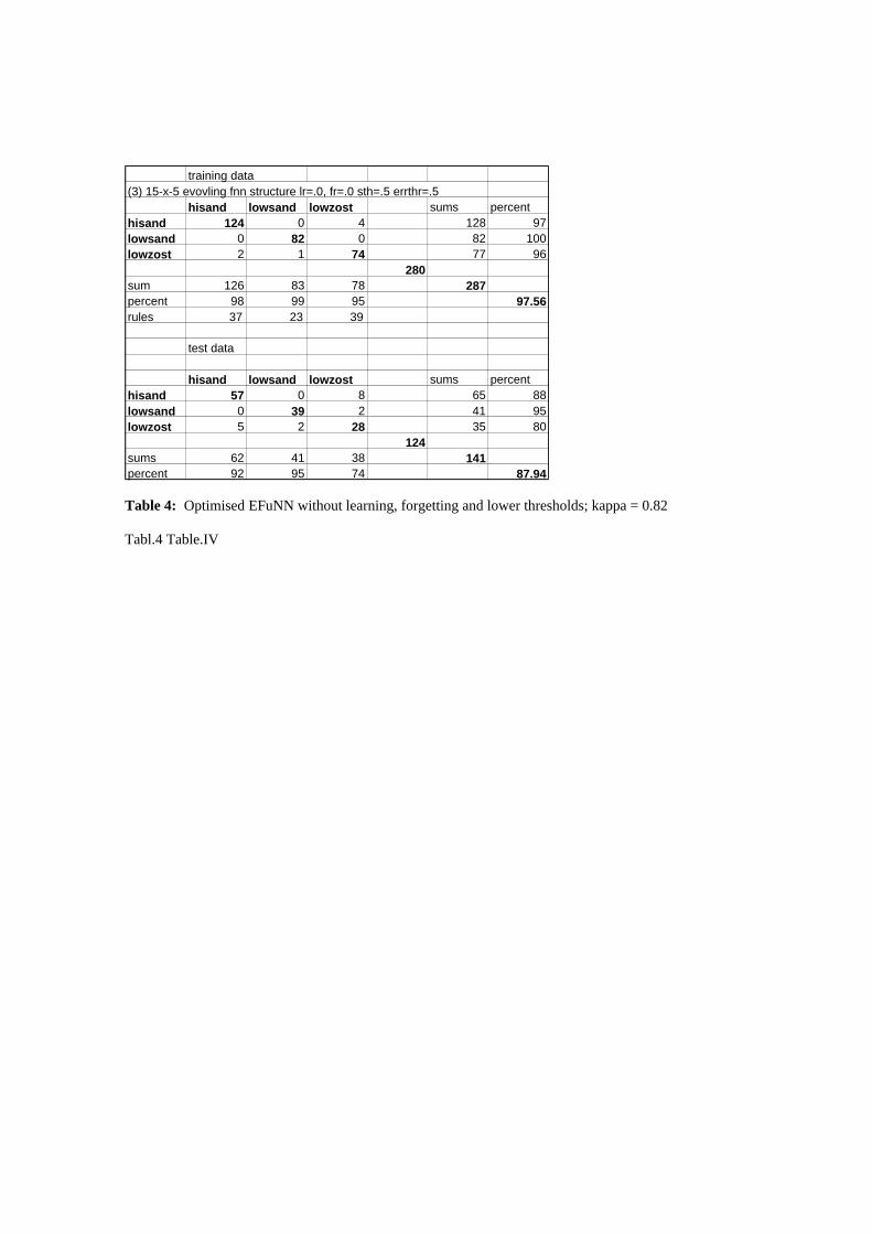
slightly (kappa = 0.82;Table 4). However, when learning and forgetting were applied to the initial condi-

tions mapping precision decreased (kappa = 0.57; Table 5). The age parameter added considerable vola-

tility to the analysis as reduced age made the network for lowsand unstable. However, when applied to

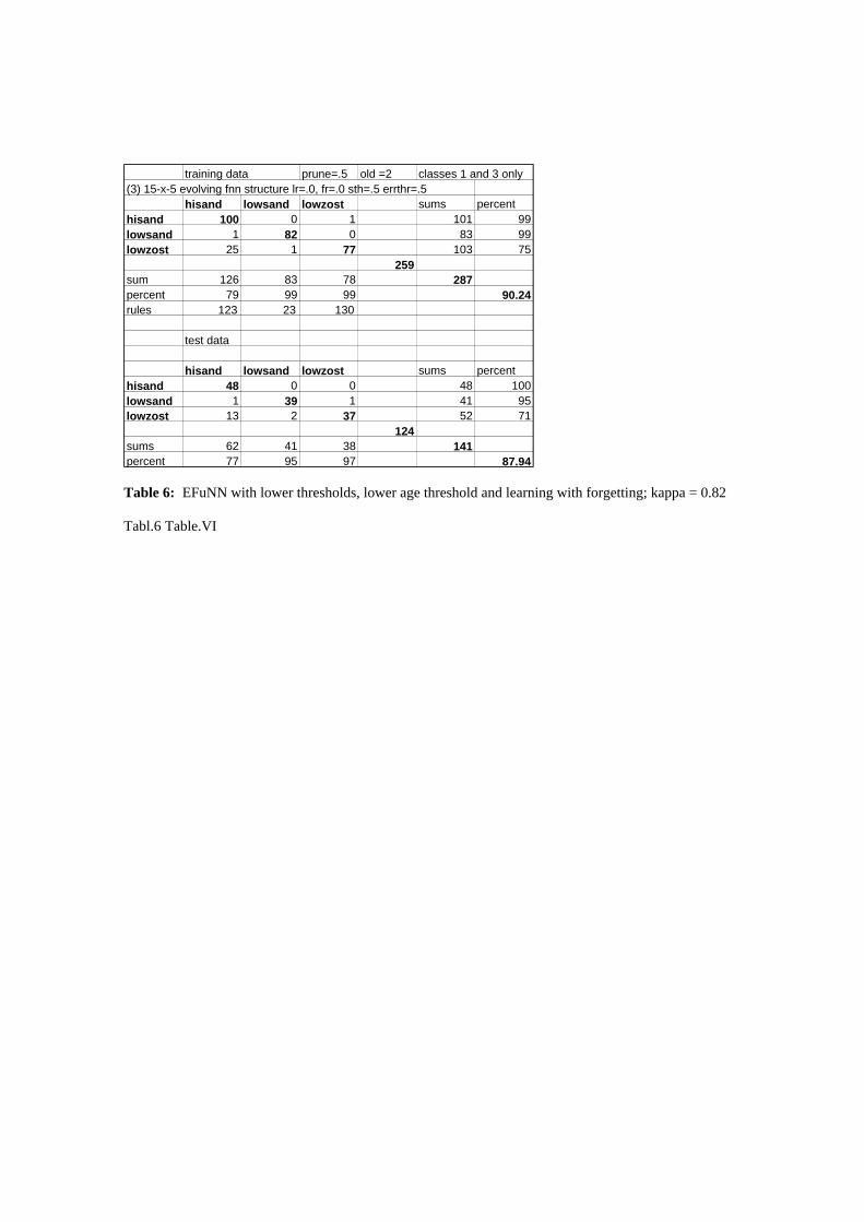
the hisand and lowzost networks, mapping error was maintained (kappa = 0.82; Table 6).

Table.I

Table.II

Table.III

Table.IV

Table.V

Table.VI

3.5. Discussion and Future Research

The important advantage evolving systems is that comparable mapping accuracies can be obtained with a

single iteration, reducing computational time. The FuNN for the same three classes required a total of

700 iterations while the EFuNN required three. The structure of the EFuNN is also optimised to reduce

the computational burden because not all nodes are recomputed for each training example. This is be-

cause EFuNNs are locally tuned for each example (only one rule node is tuned) while FuNNs require

changing all the connection weights for each example.

Future work will be conducted in order to apply the EFuNN to cases of block sampled imagery. Block

sampling is fast to acquire but spatial variations make the population distribution unknown. For those

regions on the image where the classification performance is unsatisfactory, new blocks are sampled and

those specific discriminant functions are updated.

Other experiments will allow connections to cross between EFuNNs to force training on correlated exam-

ples to occur in parallel. In this manner, the evolving of a given EFuNN could be based upon a system

wide approach as developed in the learning techniques for the FuNN. These networks also have the ca-

pability to incorporate additional attributes and outputs into the existing network structure. This is im-

portant when new information, such as new imagery or additional spectral bands become available.

Likewise the analyst is able to identify new output classes to better distinguish among the data.

4. Case Study 2: Fruit Quality Assurance Based on Image Analysis

4.1. Introduction

The application of neuro-fuzzy techniques for object recognition has been extensively studied

3,7,11,13,,24,30,34,36,39). One area where these techniques have rarely been applied is in horticultural research,

specifically for the analysis of damage to pip fruit in orchards with the goal of identifying what pest

caused the damage. The result of this application could become part of a larger computer based system

which allows the user to make better informed decisions improving the quality of the fruit produced.

Each insect or insect group has specific characteristics which allow it to be identified by the damage to

the fruit and/or leaves or the by-products of that damage. Once the insect has been successfully identi-

fied, the appropriate treatment can be applied. Examples of the type of damage are presented below. All

the images were in colour, taken at different orientations, lighting conditions, and sometime contained

more than one piece of fruit on the tree. Furthermore the damage to the fruit itself was of varying size

and shape. There were a total of 90 images taken of the damage of three different types of pest (Figure 5,

Figure 6, and Figure 7).

Fig.V

Fig.VI

Fig.VII

Successful analysis of the fruit damage requires a technique that copes with the differences in the images

and still extracts the relevant features to allow positive identification of the pest. Using Daubechies

wavelets for image analysis and comparison has been proved to be a successful technique in the analysis

of natural images 37,38). They can characterise the colour variations over the spatial extent of the image

that can provide semantically meaningful image analysis. The output of the wavelet analysis could then

become input to a Fuzzy Neural Network (FuNN) or Evolving Fuzzy Neural Network (EFuNN).

4.2. Sampling Image Data for the Experiment

To generate a dataset to train an EFuNN or FuNN, the three band RGB image data was converted to HSI

representation. A 4-layer 2D fast wavelet transform was then computed on the intensity component of

each image. Extracting a sub-matrix of size 16x16 from each intensity component resulted in a vector of

256 attributes. The lower frequency bands normally represent object configuration in the images and the

higher frequency bands represent texture and local colour variation.

4.3. Architecture of the FuNN Classification System

The entire classification system was comprised of either 5 FuNNs to reflect the five different types of

damage that could be expected: FuNN-alm-l (FuNN to classify appleleaf curling midge leaf damage),

FuNN-alm-f (FuNN to classify appleleaf curling midge fruit damage), FuNN-cm (FuNN to codling moth

fruit damage), FuNN-lr-l (FuNN to classify leafroller leaf damage), and FuNN-lr-f (FuNN to classify lea-

froller fruit damage(.

The architecture of each FuNN had 256 inputs, 1792 condition nodes, (7 membership functions per input)

50 rule nodes, two action nodes, and 1 output. 67 images were used as the training dataset and 23 images

were used to test the classification system. The 67 images were broken down into: 10 images of appleleaf

curling midge leaf damage, 4 images of appleleaf curling midge fruit damage, 22 images of codling moth

damage, 11 images of leafroller leaf damage, and 20 images of leafroller fruit damage.

The reason for the small number of images used in the experiment is due to the unavailability of stored

electronic images of pest damage. Each FuNN in the classification system was trained with all 67 images

and the output value for the output node was changed depending on what each network was required to

learn. For example the FuNN-alm-l was trained to return 1 from the output vector for any image that had

appleleaf curling midge leaf damage and return 0 from the output vector for all the rest of the images.

After presenting the image data to each FuNN in the classification system 1000 times, the entire system

was tested on the 23 test images. Results of the confusion matrix are shown in Table 7.

Table.VII

Recalling the FuNN on the training data resulted in a 100% successful classification. When the 23 test

images were originally tested on the FuNNs, there were only slightly more than a third correctly classified

(34.78%). Although the classification accuracy was low, as damage belonging to the fruit or leaves was

correctly identified but what pest caused that damage was incorrectly identified. Fine tuning of the

FuNN’s parameters or increasing the number of membership functions to account for the subtle differ-

ences in damage particularly from appleleaf curling midge and leafroller warrants further investigation. It

is also inevitable that more images of damaged fruit are needed and have to be taken and used in future

experiments with FuNNs. But using EFuNNs, on the same small data sets, produce nearly a twice higher

test recognition and is a lot faster, as it is explained in the next section.

4.4. Architecture of the EFuNN Classification System

Logically the next step was to train a set of 5 EFuNNs on the same image data and compare the results to

that of the FuNNs. The experiment associated with EFuNN was designed to replicate the performance of

a conventional FuNN while highlighting its improved speed and demonstrate the EFuNN’s capabilities to

improve classification performance. The same set of 67 images were used on a set of five EFuNNs with

parameters of Sthr=0.95 and Errthr=0.01. The EFuNN was trained for one epoch. The number of rule

nodes generated (rn) after training was as follows: EFuNN-alm-l: rn=61, EFuNN-alm-f rn=61, EFuNN-

cm: rn=51, EFuNN-lr-l: rn=62, and EFuNN-lr-f: rn=61. The results of the confusion matrix are presented

in Table 8.

Table.VIII

4.5. Results

It appears that the EFuNNs (60%) are significantly better at identifying what pest has caused the damage

to the fruit than the FuNNs (35%). Computing the kappa coefficient for both the FuNN and EFuNN con-

fusion matrixes substantiates this with results of 0.10 for the FuNN and 0.45 for the EFuNN. Yet under a

Z Test at 95% the results are not statistically significant as the size of the data sets is not statistically suf-

ficient. Further experiments are planned with a greater quantity of image data.

5. Discussion

The paper suggests a methodology for classification of images based on fuzzy neural networks (FuNNs)

and evolving fuzzy neural networks (EFuNNs). EFuNNs merge three AI paradigms: connectionism;

fuzzy rule-based systems; and case-based reasoning. The methodology has been illustrated on two case

studies – data taken from satelite images, and image data from fruit. The methodology proves to be ef-

fective in terms of fast adaptive learning for image classification.

EFuNNs have features that make them suitable for image classification when large feature space, and/or

large databases are utilised. These features are 19-23):

(1) local element training and local optimisation;

(2) fast learning (possibly one pass);

(3) achieving high local or global generalisation in an on-line learning mode;

(4) memorising exemplars for a further retrieval or system’s improvement;

(5) interpretation of the EFuNN structure as a set of fuzzy rules as explained in 23).

(6) dynamical self-organisation achieved through growing and pruning.

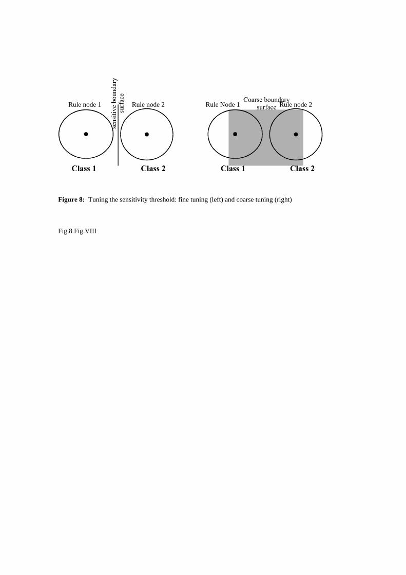
The strength of EFuNNs centres around tuning the sensitivity threshold. The sensitivity threshold acts as

a minimum resolvable distance or radius r around the rule nodes. As the sensitivity increases, the bound-

ary surface separating two acceptance regions in the feature space reduces (Figure 8). If an example from

Class 1 is defined as x and Class 2 as x’, then d = x – x’ < r for discrimination. One obvious outcome of

this research is the development of a dynamic architecture that can tune the sensitivity threshold without

operator intervention. Lower sensitivity thresholds promote stability, generalisation, and computationally

efficiency , while higher sensitivities increase discrimination.

Fig.VIII

Acknowledgements

This work was partially supported by the research projects UOO808 and HR0809 funded by the Founda-

tion of Research, Science and Technology of New Zealand. The initial funding for the ground reference

survey and baseline environmental research was provided by the New Zealand Department of Conserva-

tion, Otago Conservancy. The SPOT imagery was purchased through a grant from the New Zealand

Lottery Board. The fruit image data is owned by HortResearch, New Zealand. The authors thank Dr.

Howard Wearing for his help to obtain and analyse these images.

6. References

1. S. Amari and N. Kasabov (eds.), “Brain-Like Computing And Intelligent Information Systems,”

Springer Verlag, Berlin, (1997).

2. J. Bezdek, “Pattern recognition with fuzzy objective function algorithms,” New York, Plenum Press,

(1981).

3. J.J. Buckley and Y. Hayashi, “Are regular Fuzzy Neural Nets Universal Approximators?,” Proc. In-

ternational Journal Conference on Neural Networks (IJCNN), 721-724, (1993).

4. J.J. Buckley and Y. Hayashi, “Hybrid neural nets can be fuzzy controllers and fuzzy expert systems,”

Fuzzy Sets and Systems, 60, 135-142, (1993).

5. G. Carpenter and S. Grossberg, “Pattern Recognition By Self-Organising Neural Networks,” MIT

Press, Cambridge, Massachusetts, (1991).

6. R.G. Congalton, R.G. Oderwald and R.A. Mead, “Assessing Landsat Classification Accuracy using

Discrete Multivariate Analysis Statistical Techniques,” Photogrammetric Engineering and Remote

Sensing, 49-12, 1671-1678, (1983).

7. D. Fischer, P. Kohlhepp and F. Bulling, “An Evolutionary Algorithm for the registration of 3-D Sur-

face Representations,” Pattern Recognition, 32-1, 53-96, (1999).

8. G.M. Foody, “Sharpening Fuzzy Classification Output to Refine the Representation of Sub-Pixel

Land Cover Distribution,” International Journal of Remote Sensing, 19-13, 2593-2599, (1998).

9. S. Grossberg, “Studies of Mind and Brain,” Reidel, Boston, (1982).

10. M.M. Gupta and D.H. Rao, “On the Principles of Fuzzy Neural Networks,” Fuzzy Sets and Systems,

61-1, 1-18, (1994).

11. S.A. Israel and N.K. Kasabov, “Statistical, Connectionist, and Fuzzy Inference Techniques for Image

Classification, “ SPIE Journal of Electronic Imaging, 6-3, 337-347, (1997).

12. R. Jang, “ANFIS: Adaptive Network-Based Fuzzy Inference System,” IEEE Trans. on Syst., Man,

Cybernetics, 23-3, May-June 1993, 665-685, (1993).

13. B. Jose, B.P. Singh, S. Venkataraman and R. Krishnan, “Vector Based Image Matching for Indexing

in Case Based Reasoning Systems,” 4th German Workshop on Case-based Reasoning-System De-

velopment and Evaluation, Berlin, 7 pages, (1996).

14. N. Kasabov, “Foundations of Neural Networks, Fuzzy Systems and Knowledge Engineering,” The

MIT Press, Cambridge, Massachusetts, (1996).

15. N. Kasabov, “Learning fuzzy rules and approximate reasoning in fuzzy neural networks and hybrid

systems,” Fuzzy Sets and Systems 82-2, 2-20, (1996).

16. N. Kasabov, J. S. Kim, M. Watts and A. Gray, “FuNN/2- A Fuzzy Neural Network Architecture for

Adaptive Learning and Knowledge Acquisition,” Information Sciences – Applications, 101(3-4),

155-175, (1997).

17. N. Kasabov, “The ECOS Framework and the ECO Learning Method for Evolving Connectionist

Systems,” Journal of Advanced Computational Intelligence, 2-6, 195-202, (1998).

18. N. Kasabov, “ECOS: A Framework For Evolving Connectionist Systems And The Eco Learning

Paradigm,” Proceedings of ICONIP'98, Kitakyushu, 1232-1237, (1998).

19. N. Kasabov, “Evolving Fuzzy Neural Networks - Algorithms, Applications and Biological Motiva-

tion,” in Proc. of Iizuka'98, Iizuka, Japan, 217,274, (1998).

20. N. Kasabov, “Evolving Connectionist And Fuzzy Connectionist System For On-Line Decision

Making And Control,” in: Soft Computing in Engineering Design and Manufacturing, Springer Ver-

lag, (1999).

21. N. Kasabov, ”Evolving Connectionist and Fuzzy-Connectionist Systems: Theory and Applications

for Adaptive, On-line Intelligent Systems,” in: N. Kasabov and R. Kozma (eds) “Neuro-fuzzy Tools

and Techniques for Intelligent Systems,” Springer Verlag (Physica Verlag), 111-144, (1999).

22. N. Kasabov, “Evolving Connectionist Systems: Principles and Applications,” Technical Report, TR

99-02, Department of Information Science, University of Otago, (1999).

23. N. Kasabov, “Rule extraction, rule insertion, and reasoning in Evolving Fuzzy Neural Networks,”

Submitted to Neurocomputing, (1999).

24. D.A. Kerr and J.C. Bezdeck, “Edge Detection Using a Fuzzy Neural Network,” Science of Artificial

neural Networks, SPIE, Orlando, Florida, 1710, 510-521, (1992).

25. T. Kohonen, “The Self-Organizing Map,” Proceedings of the IEEE, 78-9, 1464-1497, (1990).

26. T. Kohonen, “Self-Organizing Maps,” second edition, Springer Verlag, Berlin, (1997).

27. T. Kohonen, “An Introduction to Neural Computing, Neural Networks,” 1-1, 3-16, (1988).

28. B. Kosko, “Fuzziness vs. probability,” in “Fuzzy and Neural Systems: A dynamic System to Machine

Intelligence”, Prentice-Hall, Englewood Cliffs, NJ, 263-298, (1992).

29. T.M. Lillesand and R.W. Kiefer, “Remote sensing and image interpretation,” (3rd ed), Thomas Wiley

and Sons, New York, (1994).

30. M. Meneganti, F.S. Saviello, and R. Tagliaferri, “Fuzzy Neural Networks for Classification and De-

tection of Anomolies,” IEEE Transactions on Neural Networks, 9-5, 848-861, (1998).

31. K. Nozaki, H. Isibuchi and H. Tanaka, “A simple but powerful heuristic method for generating fuzzy

rules from numerical data,” Fuzzy Sets and Systems, 86, 251-270, (1997).

32. S. K. Pal and S. Mitra, “ Multilayer Perceptron, Fuzzy Sets, and Classification,” IEEE Transactions

on Neural Networks, 3-5, 683-697, (1992).

33. L .I. Perlovsky, “Computational Concepts in Classification: Neural Networks, Statistical Pattern

Recognition, and Model-Based Vision,” Journal of Mathematical Imaging and Vision, 4-1, 81-110,

(1994).

34. K.S. Ray and J. Ghoshal, “Neuro Fuzzy Approach to Pattern Recognition,” Neural Networks, 10-

1,161-182, (1997).

35. D. Ruan and E.E. Kerre, “Fuzzy implication and generalized fuzzy method of cases,” Fuzzy Sets and

Systems, 54, 23-37, (1993).

36. L. Shen and H. Fu, “Principal Component based BDNN for Face Recognition,” Proceedings of the

1997 International Conference in Neural Networks (ICNN '97), 1368-1372, (1997).

37. J.Z. Wang, G. Weiderhold, O. Firschien, and X.W. Sha, “Wavelet-based Image Indexing Techniques

with Partial Sketch Retrieval Capability,” Proceedings of the Fourth Forum on Research and Tech-

nology Advances in Digital Libraries (ADL’97), 13-24, (1997).

38. J.Z. Wang, G. Weiderhold, O. Firschien, and X.W. Sha, “Applying Wavelets in Image Database Re-

trieval,” Technical Report, Stanford University, (1996).

39. T. Whitford, C. Matthews, and I. Jagielska, “Automated Knowledge Acquisition for a Fuzzy Classi-

fication Problem,” Proceedings of the Artificial Neural Networks and Expert Systems Conference

(ANNES’95), Dunedin, New Zealand, IEEE Press, 227-230, (1995).

40. D.H. Wolpert, “On the Connection Between In-Sample Testing and Generalization Error,” Complex

Systems, 6, 47-94, (1992).

41. L.A. Zadeh, “Fuzzy Sets,” Information and Control, 8, 338-353, (1965).

Figure 1: A FuNN structure of 2 inputs (input variables), 3 fuzzy linguistic terms for each variable (3

membership functions). The number of the rule (case) nodes can vary. Three output membership func-

tions are used for the output variable.

Figure 2: Two Class Feature Space where Acceptance Regions Vary with Time: Initial State (solid),

Adapted Stated (dotted). The distances between class centers are represented by lines.

Figure 3: Scatterplot of 3 Ambiguous Classes (infrared versus reflectance as green inputs).

Figure 4: Scatterplot of 3 Ambiguous Classes (red versus reflectance as green inputs).

Table 1: Maximum Likelihood Classifier (MLC) (Bayes rule); kappa = 0.84

Table 2: FuNN without learning techniques; kappa = 0.80

Table 3: Initial EFuNN for three confused landcover classes; kappa 0.80

Table 4: Optimised EFuNN without learning, forgetting and lower thresholds; kappa = 0.82

Table 5: EFuNN with leaning and forgetting; kappa = 0.57

Table 6: EFuNN with lower thresholds, lower age threshold and learning with forgetting; kappa = 0.82

Figure 5: Examples of codling moth damage

Figure 6: Examples of appleleaf curling midge damage

Figure 7: Examples of leafroller damage

Table 7: FuNN with learning and forgetting; kappa=0.10

Table 8: EFuNN with learning and forgetting; kappa = 0.45

Figure 8: Tuning the sensitivity threshold: fine tuning (left) and coarse tuning (right)

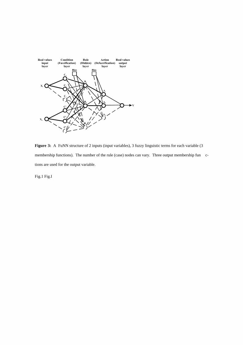
Figure 3: A FuNN structure of 2 inputs (input variables), 3 fuzzy linguistic terms for each variable (3

membership functions). The number of the rule (case) nodes can vary. Three output membership func-

tions are used for the output variable.

Fig.1 Fig.I

t: time movement

t+n, t+m: following time movements

Figure 4: Two Class Feature Space where Acceptance Regions Vary with Time: Initial State (solid),

Adapted Stated (dotted). The distances between class centers are represented by lines.

Fig.2 Fig.II

t+m t+n

t t

0.2

0.25

0.3

0.35

0.4

0.45

0.1 0.15 0.2 0.25

infrared

gre

en

hisand

lowsand

lowzost

Figure 3: Scatterplot of 3 Ambiguous Classes (infrared versus reflectance as green inputs).

Fig.3 Fig.III

0.2

0.25

0.3

0.35

0.4

0.45

0.1 0.15 0.2 0.25 0.3 0.35

red

gre

en

hisand

lowsand

lowzost

Figure 4: Scatterplot of 3 Ambiguous Classes (red versus reflectance as green inputs).

Fig.4. Fig.IV

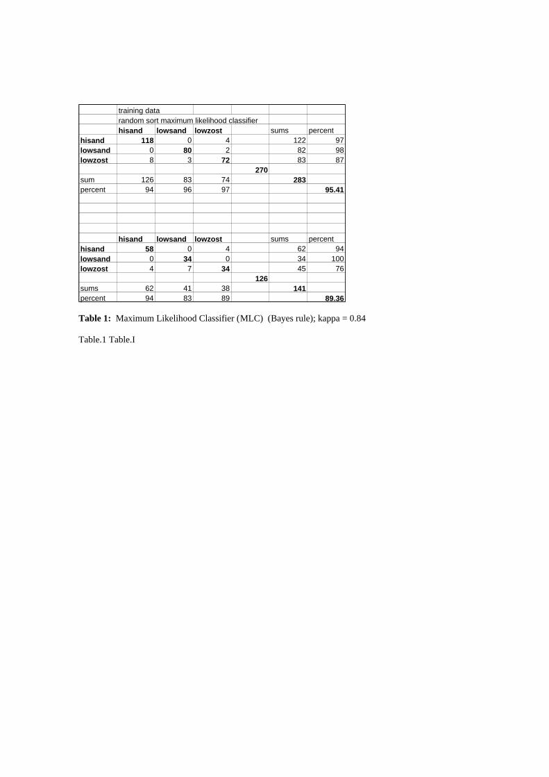
training datarandom sort maximum likelihood classifierhisand lowsand lowzost sums percent

hisand 118 0 4 122 97lowsand 0 80 2 82 98lowzost 8 3 72 83 87

270sum 126 83 74 283percent 94 96 97 95.41

hisand lowsand lowzost sums percenthisand 58 0 4 62 94lowsand 0 34 0 34 100lowzost 4 7 34 45 76

126sums 62 41 38 141percent 94 83 89 89.36

Table 1: Maximum Likelihood Classifier (MLC) (Bayes rule); kappa = 0.84

Table.1 Table.I

training datarandom sort (3) 15-10-2 fuzzy neural networks in parallel


271sum 126 83 78 287percent 92 96 96 94.43iterations 200 200 300

test data


123sums 62 41 38 141percent 85 80 97 87.23

Table 2: FuNN without learning techniques; kappa = 0.80

Table.2 Table.II

training data(3) 15-x-5 evolving fuzzy neural networks structure


274sum 126 83 78 287percent 95 99 92 95.47rules 279 279 279sthr=0.95 errthr=.001 lr=0.05 prune=0.1 fgr=0.01

test data


123sums 62 41 38 141percent 94 85 79 87.23

Table 3: Initial EFuNN for three confused landcover classes; kappa 0.80

Table.3 Table.III

training data(3) 15-x-5 evovling fnn structure lr=.0, fr=.0 sth=.5 errthr=.5


280sum 126 83 78 287percent 98 99 95 97.56rules 37 23 39

test data


124sums 62 41 38 141percent 92 95 74 87.94

Table 4: Optimised EFuNN without learning, forgetting and lower thresholds; kappa = 0.82

Tabl.4 Table.IV

training data(3) 15-x-5 EFuNN structure lr=.1, fr=.1, sthr =.95, ethr = .05



test data


100sums 62 41 38 141percent 77 34 100 70.92

Table 5: EFuNN with leaning and forgetting; kappa = 0.57

Tabl.5 Table.V

training data prune=.5 old =2 classes 1 and 3 only(3) 15-x-5 evolving fnn structure lr=.0, fr=.0 sth=.5 errthr=.5



test data


124sums 62 41 38 141percent 77 95 97 87.94

Table 6: EFuNN with lower thresholds, lower age threshold and learning with forgetting; kappa = 0.82

Tabl.6 Table.VI

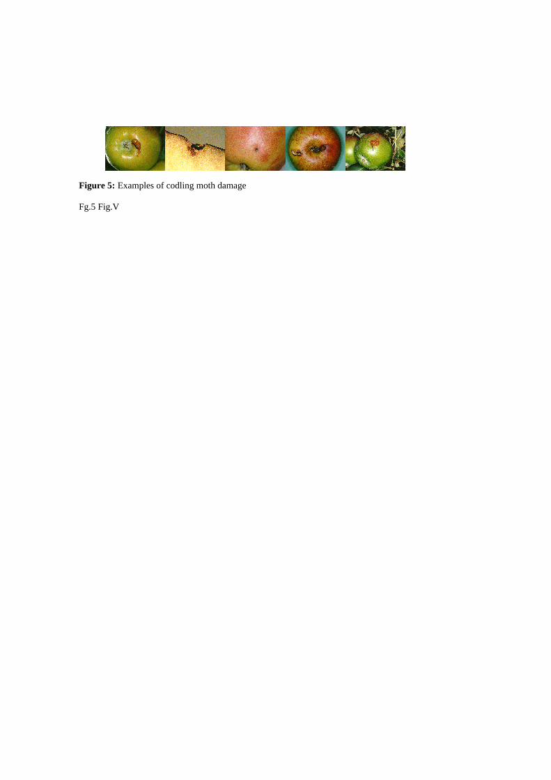
Figure 5: Examples of codling moth damage

Fg.5 Fig.V

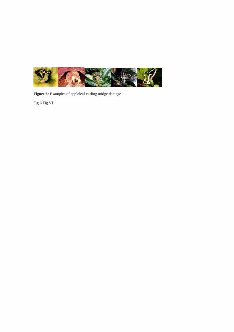
Figure 6: Examples of appleleaf curling midge damage

Fig.6 Fig.VI

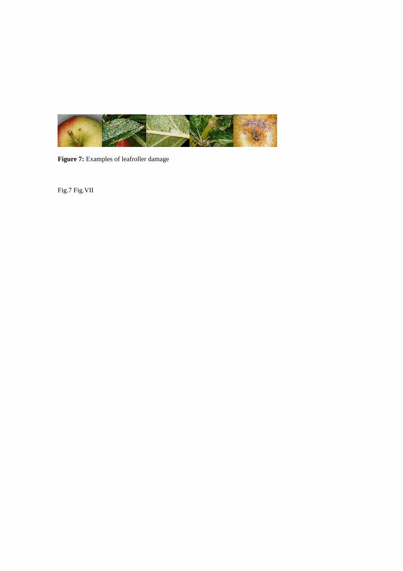
Figure 7: Examples of leafroller damage

Fig.7 Fig.VII

training data - 5 fuzzified networks 256-1792-50-2-1 in parallelmaximum of 1000 iterations or 0.00001 error.

alm-l alm-f cm lr-l lr-f sums percentam-l 9 0 0 0 0 9 100alm-f 0 5 0 0 0 5 100cm 0 0 22 0 0 22 100lr-l 0 0 0 16 0 16 100lr-f 0 0 0 0 15 15 100

67sum 9 5 22 16 15 67percent 100 100 100 100 100 100iterations 1000 1000 1000 1000 1000

test dataalm-l alm-f cm lr-l lr-f sums percent

am-l 1 0 0 0 0 1 100alm-f 0 1 0 0 0 1 100cm 2 1 3 2 2 10 30lr-l 0 0 2 1 0 3 33lr-f 0 0 4 2 2 8 25

8sum 3 2 9 5 4 23percent 33 50 33 20 50 34.78

Table 7: FuNN with learning and forgetting; kappa=0.10

Table.7 Table.VII

training data5 eFunns lr=0.0 pune=0.1 errth=0.01 sthr=0.95 fr=0.

alm-l alm-f cm lr-l lr-f sums percentam-l 9 0 0 0 0 9 100alm-f 0 5 0 0 0 5 100cm 0 0 22 0 0 22 100lr-l 0 0 0 16 0 16 100lr-f 0 0 0 0 15 15 100

67sum 9 5 22 16 15 67percent 100 100 100 100 100 100.00rule nodes 61 61 61 62 61

test dataalm-l alm-f cm lr-l lr-f sums percent

am-l 2 0 1 1 0 4 50alm-f 0 1 0 0 0 1 100cm 1 1 7 1 2 12 58lr-l 0 0 0 2 0 2 100lr-f 0 0 1 1 2 4 50

14sum 3 2 9 5 4 23percent 67 50 78 40 50 60.87

Table 8: EFuNN with learning and forgetting; kappa = 0.45

Table.8 Table.VII

Rule node 1 Rule node 2 Rule Node 1 Rule node 2

Figure 8: Tuning the sensitivity threshold: fine tuning (left) and coarse tuning (right)

Fig.8 Fig.VIII

The Application of Hybrid Evolving Connectionist Systems to Image ...

Documents

Transcript of The Application of Hybrid Evolving Connectionist Systems to Image ...