vvThe Analytic Continuations of Distributions t f

Dissertation

Submitted to the School of Mathematics of

The University of Nairobi

(Division of Pure Mathematics)

by

ONGARO, JARED NYANG’AU

In partial fulfillment of the requirements

for the Degree of

Master of Science in Pure Mathematics.

University of NAIROBI Library

I 37898I 5

©August 2009

Declaration

I the undersigned declare that this dissertation is my original work and to the best o f my

knowledge has not been presented for the award o f a degree in any other University.

O N G ARO JAR E D N Y A N G ’AU

Reg. No. 156/71571/2(X)7

Declaration by Supervisors

This dissertation has been submitted for examination with my approval as a supervisor

C LA U D IO AC H O LA

Signature Date

Date

To my girlfriend; Lilian Kerubo

who has adjusted extremely well to having a mathematician as boyfriend.

On Analytic Continuations of Distributions

ONGARO JARED NYANG’AU

August 7, 2009

Abstract

In this dissertation, we develop the elements necessary at providing the theoretical formulation of

the solution to the Gel’fand(1954) problem. All the results are well-known and our contribution

is only at the level of the presentation.

Suppose K is a field of characteristic 0; for instance, take K = K . Given p { x ) G R [x i , • • • , Xn \,

A G C, |p(x)|^ is well defined for R e (A) > 0 on R n. Can we analytically continue |/?(x)|

to the entire complex plane? This is the problem of I. M. Gel’fand, posed at the International

Congress o f Mathematicians, Amsterdam 1954.

In 1968, Bernstein and S. I. Gel’fand [7| and Atiyah [11|, independently provided a solution with

proofs of this fact based on Hironaka’s theorem about resolution of singularities, a very deep and

difficult result. However, in 1972, Bernstein produced a beautiful and a completely algebraic proof

of the result. The idea of the proof is; to analytically continue |p(x)| we can use Bernstein-Sato

polynomial 6(A), which has the property that

b (\ ) p ( x )X~ l = ( some polynomial differential operator ) p ( x ) \

We pick up poles from the zeros of 6(A) (the poles of the analytic continuation will be at integer

shifts of the zeros of 6(A), since we have to repeat the process). To compute this polynomial is

an involving process as seen in example 3.3.8. Fortunately, we do not always need to know 6 (A )

explicitly. Bernstein showed how to prove that it exists, without actually producing it.

The problem is best considered in the context of distributions. Thus, in this dissertation the

basic concepts of distribution are used and the modern theory of distribution as introduced by

Laurent Schwartz is explained. Some powerful algebraic machinery: D-module theory is then

introduced. Finally, we shown how a problem of analysis with complicated solution can be solved

through algebraic approach with relative ease.

i

Table of Contents

A bstract................................................................................................................................ i

Acknowledgements............................................................................................................... iv

Notation ............................................................................................................................. vi

1 In trodu ction 1

1.1 Historic Rem arks........................................................................................................ 1

1.2 Motivation for D-Modules ....................................................................................... 2

1.3 Some Function Theory on Complex Domains............................................................ 3

1.4 Analytic Continuation of a function.......................................................................... 4

2 D istribu tions T h eo ry 6

2.1 In trodu ction ............................................................................................................... 6

2.2 What good are distributions?.................................................................................... 7

2.3 Formal Definition of Distributions .......................................................................... 11

2.4 Topology and Convergence of Test F u n ction s ......................................................... 13

2.5 The Derivative of a Distribution ............................................................................. 17

2.5.1 Approximation of distributions using test functions .................................. 19

3 T h e A n a ly tic Continuation o f D istribu tions 20

3.1 Introduction............................................................................................................... 20

3.2 Further D evelopm ent.................................................................................................. 21

3.3 The Analytic Continuation Problem........................................................................... 21

4 A Quick In troduction to D -m odule T h e o ry 26

ii

4.1 The Weyl A lg e b r a ..................................................................................................... 26

4.2 Grading and Filtrations ........................................................................................... 28

4.2.1 Filtration of A n modules................................................................................ 30

4.3 Dimensions and M ultiplicities.................................................................................... 31

4.4 Holonomic modules ................................................................................................. 35

5 T h e Bernstein -Sato polynom ia ls 36

5.1 Existence of Bernstein-Sato polynom ia l................................................................... 39

5.2 Solution of the Analytic Continuation P ro b le m ........................................................ 40

5.3 Conclusion................................................................................................................... 42

R e fe r e n c e s ......................................................................................................................... 43

I n d e x ................................................................................................................................... 44

iii

Acknowledgements

I am proud to have benefited from the patience, quiet wisdom of my core supervisor here at

Nairobi, Claudio Achola. His encyclopedic knowledge, coupled with his considerable shrewdness

and topped by his understanding and kindness, make him a role model both professionally and

personally. Many thanks to Claudio (again) was my research mentor at the University of Nairobi;

like all excellent teachers, not only his knowledge but his tastes proved contagious, and I am a

better mathematician for it. He was often able to explain things from a point o f view which

rendered a difficult problem much clearer. This was a great help when trying to wade through a

junk o f well written but at times very complicated texts on the subject. I can’t describe what he

has given me, I will always admire Claudio, for his mathematical mind, but aside from that, for

his generosity, kindness and his way of life. I have never learn’t more on anything from anybody

else, and I doubt I ever will.

My second supervisor, lecturer and a friend James Nkuubi: James never stopped encouraging me

in this work. Not only his commitment in mathematics, but, flexibility and availability makes him

a person I couldn’t avoid working with at this level. Thanks! James, through this work I have

learned to appreciate the power and beauty of D-modules.

Many Thanks to Professor Rikard Bogvad for suggesting the topic and structure of the disser­

tation when we met,(April ’09) during the EAUM P school on Set theory and Logic in Nairobi

and making sure none of my mails went unreplied. He showed continued interest in my work and

has given me valuable suggestions for corrections and improvements. I can only hope I didn’t

disappoint!. So to the entire Algebraic analysis group in Nairobi-Stock holm Claudio and Rikard,

thank you!. To Madam Anne who will have been my third supervisor would it have been not

what it was?! The tea, peanuts and hot dogs at the Chiromo club was refreshing and proved to

be very important due to discussion which we engaged in with the senior members of the club:

will truly miss the tea. People like Dr. Patrick Weke, could have said more if I was particularly

more organised like him. Patrick, that is the way it should be.

My work become easier after I acquired a grant to buy a Laptop from African Millennium Math­

IV

ematics Initiative(AMM SI), special thanks to tlie Director Professor YVandera Ogana. I wish to

thank the School of Mathematics and the entire University of Nairobi, particularly, thanks to

Professor John Okoth Owino for Initiating unfamiliar programme which I really benefited from.

Things were not that easy after his departure as director of the school, but we were lucky that

his passion for mathematics, made him rest our case to then incoming director; who renewed our

scholarship without much ado. I acknowledge you; Dr. Hudson Were. To my opinion, the Division

of Pure mathematics was organised thank to the leadership of Professor Khalagai. I should also

point out that the much analysis you will encounter in this dissertation credit to him; He always

taught expressing a lot of mathematical understanding of the underlying concepts.

Perhaps this was where to start my acknowledgments; my family, who are responsible for so much

of who I am today. I am grateful to them for all o f their love and support, and for only occasionally

asking "what is all this good for anyway?". I love you all immensely. I could never have completed

this dissertation without help in both mathematics and support from my greatest inspiration of

all times ever since we joined university; my dearest friend Benjamin Kikwai, who helped inspire

me. To all my other classmates Edwin, Presly, Dennis, Faith and Ester who put up with my

frustrations and who continuously supported me; you are God sent. I would not have made it

through the past two years without your encouragement, I thank you.

Finally, I would like to thank my high school mathematics teacher Peter Kirenge for getting me

interested in mathematics to begin with. Mr. Kirenge, this is what that algebra became! Sim­

ilarly, I would like to acknowledge the absolute important role of Professor G.P. Pokhariyal for

his generous spirits and for having open enough minds. Pokhariyal, in response to my request to

avoid doing any Geometry courses at master level replied: I'm not going to let you out of here

with a pure mathematics degree without seeing some proper Geometry!’ . I hope this dissertation

shows that I have learnt t he basics of geometry, and Pokhariyal will let me graduate. He is such

a strict and an effective professor who makes sure every i was dotted, thank you.

ONGARO NYANG’AU

Nairobi-Kenya

August-2009.

v

Notation

These are some of the commonly used notation in our work.

C : Field of Complex numbers

R : Field of Real numbers

N : set of Positive numbers

K : Field of characteristic 0

K [ X ] = K [ x i , • • • ,Xn\'- Polynomial ring over K

A n ( K ): n ^ 1 Weyl algebra

T ) = C o °(IR n): Space of all test functions

T ) : Space of distributions on W

S ij : Kronecker delta

{ B j } : Bernstein Filtration

X = ( x i , • • • , X n ): Point in IR;'

vi

Chapter

Introduction

1.1 Historic Remarks

D-module is a module over a ring D of differential operators. The major interest of such D-

modules is as an approach to the theory of linear partial differential equations. Since around 1970,

D-module theory has been built up, mainly as a response to the ideas of Mikio Sato on algebraic

analysis and as an expansion on the work of Sato and Joseph Bernstein on the Bernstein-Sato

polynomials. Therefore, there has been a vast amount of work on the theory of D-modules over the

past 30 years, particularly due to the contributions of I.N. Bernstein, J. E. Bjork, M. Kashiwara,

T. Kawai, B. Malgrange, Z. Mebkhout, and others.

Question 1.1.1. Why D-modules ?

As Coutinho points out in his book [1], the question is particularly easy to answer. Hardly any area

of Mathematics has been left untouched by this theory: from Number Theory to Mathematical

Physics and from Singularity Theory to Representation of Algebraic Groups, to mention only a

bunch. Indeed, the theory o f D-modules sits across the traditional division into Algebra, Analysis

and Geometry and this fact gives to the theory a rare beauty.

1

1.2 Motivation for D-Modules

Let A be a field of characteristic 0. For some fixed Tl ,K\X\ denotes the polynomial ring in il

variables. A n is the sub algebra of E n d ^ K [ X ] generated by the operators

/ X i f and / 0/d x i

which are denoted by X{ and d\. We note that; A n [ x \, • • • , x n , d [ , • • • , dn ].

R em ark 1.2.1. To make the notation less cluttered we will often drop the subsci'ipts fo r the

generators of A \ and write them simply as X and d.

The Weyl algebra is simple, i.e. the only two-sided ideals of A n are 0 and A n itself. However,

A n is very rich in one-sided ideals. We denote by (P\ »* * * j P m ) the left ideal of A n generated

by the operators P \ , • • • , P m £ A n .

The left ideal / = (P\, • • • , Pm) is exactly the object one would want to examine in order

to study the system of linear partial differential equation(PDEs)

^1 * / = P2 •/ = *•* = Pm ‘ / = 0» (1-1)

where / is the unknown function. In deed, the operators of I produce equations that follow

algebraically from the equations 1.1. Now , we can quotient the ring A n by these equations, to

get a D-module.

E xam p le 1.2.2. To study the equation — ^ = 0, we would take M : = A\/ — d } .

while to study — y = 0 we would also take M := A \ j ( ( d — 1 )^ ) .

The solution of our differential equation is just a D-module homomorphism from h i to a D -

module S of functions. Note that while we arc working with algebraic differential operators,

space o f functions S is a D-module. So we can study algebraic, analytic, or smooth solutions to

our equations.

E xam p le 1.2.3. A single linear operator represented by a cyclic ideal I\ = (r) — d ) correspond

to the space of solutions spanned by functions 1, €x and e x . The solutions of ideal 12 —

( ( d — 1 )^ ) are spanned by ex and XC'1.

2

R em ark 1.2.4. Not all the ideals in the first Weyl algebra are cyclic. For example, the ideal

I = ( ( f t ) ~ l ) cannot be generated by one element; In fact, according to Stafford: Every left

ideal o f the Weyl algebra can be generated by two elements.

Clearly, K-linear space M is called a (left) D-module if there is a left action of A n defined on M .

When D-rnodules are employed to study systems of linear PDE, the first question one may ask is:

what are the solutions? The concept of the solution space is readily available in the language of

D-modules.

That is, to solve the system of equations represented by a cyclic D-module M \ = D / I in

terms of the functional space represented by D-module M 2 means to describe the set of ho-

momorphisms H o m p ( M i , M 2 ). This set has a structure of a AVlinear space. Every element

(f> € H o r r i£ ) (M \, M 2 ) is defined by its value at the coset 1 € D / I ; since 1 has to be annihi­

lated by /, it is a solution to the corresponding system of PDEs.

E xam p le 1.2.5. Consider cyclic ideals I\ = (d ^ — d ) . and ideal I 2 = ( ( d — 1 )^ ). I f S is

a space of smooth functions, then

H o r r i£ ){D / I \ , S ) = S p a n j { { l , e x , e ~ J } ,

H o m p ) (D / 1 2 , S ) = S p a r iK { e x , x e x .}

Therefore, if we look for solutions in the ring of one variable polynomials A [x], then

H o m D ( D / 1\, K\x\) = K ,

H o m D { D / I 2, K [ x ] ) * 0.

1.3 Some Function Theory on Complex Domains.

Let { } denote an open subset, called a region of the complex number space C 7/, if H is connected

then n is called a domain. Since we have a topology on C, we can talk about open sets. Just as

in real analysis, there will be domains of differentiable functions.

E xam p le 1.3.1. Let Cl be a non-empty open set in C . For instance, Q would be C itself or C

with with say finite number of points removed such as C x , or the interior of the disk, or half

plane.

3

D efin ition 1.3.2 (Holomorphic functions). They are functions defined on an open subset of com­

plex number plane C with values in C that are complex differentiable at every point. This is a

stronger condition than the real differentiability and implies that the function is infinitely often

differentiable and can be described by Taylor Series.

R em ark 1.3.3.

The term analytic function is often used interchangeably with holomorphic function, although the

term analytic is also used in broader sense of any function(real , complex or of more general type).

The fact that the class of analytic functions coincides with the class of holomorphic functions, is

a major theorem in complex analysis.

D e fin ition 1.3.4 (meromorphic functions). A meromor])hic function on an open subset f i o f the

complex plane is a function that is holomorphic on the whole o f i l , except a set of isolated points.

1.4 Analytic Continuation of a function

This is one of the most important topic in complex variable theory as used today in many physical

applications. The concept of analytic continuation just means enlarging the domain without giv­

ing up the property of being differentiable, i.e. holomorphic or meromorphic. After Weierstrass

this process is called ana lytic continuation. A ll the elementary functions of real variables may

be extended into the complex plane-replacing the real variable X by the complex variable 2. For

example, we could ask; is it possible to extend the definition of tin* sine function from the real line

to all complex numbers? This is an example of analytic continuation. Namely, the same power

series that defines the Taylor series for siil(a :) with real X, also works for complex values of X.

In general, it is a big problem in complex function theory to continue functions analytically.

E xam ple 1.4.1. The Riemann zeta-function

oo

c ( z ) = n ~ z

n— 1

is easy to define fo r complex values with real part greater than 1, but it is quite difficult to find a

continuation to the whole complex plane.

4

Q uestion 1.4.2. Why analytic continuation ?

Moving into the complex plane opens up new opportunities for analysis. It defines the analytic

functions in terms of its original definition and all its continuations. The power series met hod

described in many coffee-table books in complex analysis e.g. sec Rucl V. Churchill ct al [18| is a

common technique for doing it. However, we can also employ the integral techniques.

Generally one knows of an analytic function, such as the solution in series of a differential equa­

tion, where only the expansion around a point is usually found. However, one wants the general

function which is guaranteed to exist by analytic continuation.

5

Chapter

Distributions Theory

In this chapter, we introduce the basic notion of distributions and their properties. Some of the

uses are highlighted.

2.1 Introduction

It is true that we are used to describe the world using functions (especially physical processes in

it). Sometimes, this view gives us the connection between several different quantities: position

of an object, its speed and power applied to it is the value of a function and its first and second

derivatives. So. if we know other derivatives, one more benefit is the possibility to extrapolate the

function through Taylor series solution of differential equation. Every time we know something

quite general about the whole function, and something precise only about its behaviour on a small

set. In this manner, we can describe the function precisely everywhere by the use of derivatives.

W hy we are not happy with functions?

Sometimes functions are not differentiable. If one thinks that nondifferentiable functions exist

only in theory, it is not true. In applications one gets these as limits o f differentiable functions,

for example solving differential equation with a parameter. In many cases it is easier to consider

an nondifferentiable function(or even noncontinuous function) as a critical "the most bad " case

for differentiable function.

E xam p le 2.1.1 (Dirac delta function). The Dirac delta function on R is defined by the

6

properties

5 ( x ) =0 fo r X ^ 0, /oo

S ( x ) d x = 1.

-0000 for x = 0,

Let / be a nice function which vanishes at infinity, then,

/oo r oo poof ( x ) 6 ( x ) d x = / l / ( x ) - / ( 0 ) ] J ( x ) d x + / ( ( ) ) / S ( x ) d x = f ( 0)

-oo J —oo J —OObecause [/ (:r ) — / (0 )] (5 (x ) = 0 on IR.

( 2. 1)

There is no such function with these properties and also we cannot interpret f ( x ) 6 ( x ) d x

as an integral, in the usual sense. However, what does make sense is the assignment / i----► / (O ).

The J function is thought of as a distribution.

2.2 What good are distributions?

Theory of distributions also known as theory of generalized functionsfwe do not distinguish be­

tween these terms) was invented to give a solid theoretical foundation to the delta function S ,

which had been introduced as a technical device in mathematical formulation of quantum me­

chanics.

We now discuss some more concrete problems that will be solved in the calculus of distribu­

tions.

1. D e r iva tiv e o f discontinuous functions. One of the main achievements of 19th century

analysis was to carefully examine notions such as continuity and differentiability, and to show that

there are many continuous functions that are not differentiable.

Recall that / is differentiable at X , and its derivative is f ' ( x ) = L , if the limit

limh— >0

/ (x + h ) - } { x )

h(2.2)

exists and is equal to L .

While it was always clear that not every continuous function is differentiable, for example the

7

function / : R ► M given by f ( x ) — |x| is not differentiable at 0, it was not until the work

of Bolzano and Weierstrass that the full extent of the problem became clear: there an* nowhere

differentiable continuous functions. See Theorem 4.50 in [19].

E xam p le 2.2.1 (The Dirichlet function). The Dirichlet function is defined on R by

f 1 x € Qf ( x ) : = {

[ 0 x £ Q

every point X G K is a point of discontinuity of /.

Q uestion 2.2.2. What makes us avoid differentiating discontinuous functions? Is it because it is

impossible, unwise or simply out of ignorance?

The good news is that, what we can call as unfair restriction poised by equation 2.2, does not

prevent one from extending differentiation to continuous functions if one is willing to generalize

the class in which the result (i.e. the derivative) will lie. As we will explain, a suitable notion of

generalized functions is that of distributions. With this generalization, every continuous function,

indeed every distribution, can be differentiated as many times as desired, with the result being yet

another distribution. We will indeed generalise our concept of a function in such away that this

new specification of a function will hold for all the continuous and piecewise continuous functions.

E xam p le 2.2.3 (Heaviside step-fuiictioil). The Heaviside step-function is defined on R

as,

H ( x )0 x < 0

1 x > 0

(2.3)

then we see I I ' = 6 by Theorem 2.4.13 in the following sense. If f is a nice function which

vanishes at infinity, then integration by parts gives

8

(2.4)

[ f ( x ) H \ x ) d x = [ / ( * ) * ( * ) ] « , - rJ —x J - 00

/oo

f ' ( x ) H { x ) d x

-00/•oo

= - / f ' ( x ) d xJO

= - [ / «

= m

/oof ( x ) S ( x ) d x .

-oo2. P a rtia l D ifferen tia l Equations:

Partial differential equations have been developed as a mathematical toolbox for the description

of natural and engineered phenomena, ranging from vibrating strings to weather prediction to the

design o f the Boeing 777. Partial differential equations provide a language for modern science and

analysis provides a theoretical background for their study. Consequently, differential equations

are used to construct models of reality. Sometimes the reality we are modeling suggests that some

solutions of differential equation need not be differentiable.

Let us first fix some definition about a solution to a partial differential equation.

D efin ition 2.2.4. A partial differential equation fo r a real-valued function U in n —variables

X \, • • • , x n is a relation o f the form

f (x 1,X2, ••• ,«*, !••• = 0 (2.5)

where

U X\ —du

UX\X2 — od2u

e.t.c.rv J “ '*1X2 Odx\ ox\X2It may happen that this equation is supplemented by constraints on U and its partial derivatives of

the boundary d^l of the region f l C R n throughout which the independent variables X \, • • • , Xu

vary. These constraints are called boundary conditions, and if one of the variables is identified

as time, the constraint associated with that variable is called an initial or final condition.

D efin ition 2.2.5 (Classical solution ). A solution o f a partial differential equation is defined to be a

function u ( x \ , ..., X n ) such that all the derivatives which appear in the partial differential equation

9

exist, are continuous, and such that the equation, boundary conditions and initial conditions art-

all satisfied.

It may be thought that with this definition of a solution the main emphasis should be focused on

deriving methods by which a solution can be obtained. However, the story is not quite so simple.

If we consider the wave equation (vibrating string equation)

rj2 /~)2 Q

-Q ^ = c2 ~ f ^ ’ « ( M ) = « ( M ) = 0; « ( * . o ) = /, ^ ( x , o ) = o (2.6)

with U a function on X R j . Then the general solution of this PDE, obtained by d ’Alembert

in the 18th century, must be of the form

u ( x , t ) = f ( x + c t ) + g ( x — c t ) ,

where / and g are arbitrary functions on R . It is easy check by the chain rule that U solves the

PDE as long as we can make sense of the differentiation. So, in the classical sense, /, g twice

continuously differentiable, that is /, g 6 C ^ (R ) suffices.

Q uestion 2.2.6. But shouldn't this also work fo r rougher f , g ?

This question will be answered with the help of the following example.

E xam p le 2.2.7.

Consider / (x ) given by

J x 0 < X < ^ ,/ ( * ) = < .

1 — X 5 < x < 1,

which is equivalent to plunking a string at the mid-point. Now the solution cannot be classical

since f ( x ) is not differentiable at X = £•

Q uestion 2.2.8. So what do we mean by a solution to the problem S

It is obvious, that we must widen the concept of a solution if we are going to allow initial conditions

of the given form like in example 2.2. This restriction is both irksome and natural in many

instances. It can be overcome by introducing so called weak solutions. By definition, these are

functions U such that

Ud 2<p 2d 20 \

d t2 d x 2 Jdxd t = 0 (2.7)

10

for all sufficiently good' functions (f).

In general, idealization of physical problems often results in distributions. For instance, the

sharp front for the wave equation discussed above, or point charges (the electron is supposed to

be such!) are good examples. But a later curious application of great interest will be perhaps

the applications of Dirac’s Delta function in statistics where the ^-function approach provides us

with a unified approach in treating discrete and continuous distributions; e.g Use Delta function

to obtain discrete probability distributions see Santanu |15j.

2.3 Formal Definition of Distributions

From the foregoing, we realize that most of the time when working with ordinary functions, we

are subjected to what one might consider undesirable restrictions. In the case of differentiation,

continuous functions need not be differentiable, and a function which is once differentiable need

not be twice differentiable; similarly for Fourier integrals, all kinds of nice functions, cos X for

instance does not possess Fourier transforms.

Distributions are important in physics and engineering where many noncontinuous problems nat­

urally lead to differential equations whose solutions are distributions, such as the Dirac delta

distribution. For example, Heaviside’s mathematical innovations arising in the physics of tele­

graph cables (1880-7) were disregarded for many years. Only in the 1930s Hadamard, Sobolev,

and others made systematic use of non-classical generalized functions. In 1952, Laurent Schwartz

won a Fields Medal for systematic treatment of these ideas. In the next few sections we shall

present the basic theory of these concepts according to the latter investigator.

The suitability of a particular function of a real variable for describing physical phenomena depends

on its analytic properties such as continuity, differentiability, integrability, etc. These properties

in turn depend on the structure or topology of the underlying real number system. For instance,

to define the concept of continuity of a function of a real variable we must first investigate the

convergence of sequences of real numbers. Analogously, the analytic properties of functional must

be defined with respect to the convergence properties of sequences of functions f ( x ) o f the un-

11

derlying function space. In other words, they must be defined with respect to the structure or

topology of that function space.

Thus, the proper approach to the theory is via topological vector spaces-see Rudin’s hook [16| for

the development along these lines. Here, the underlying point set will be an n-variable space Rn

(point X = (x\, • • • , Xn ) ) or even a subset Q C Rn that is open.

Roughly speaking, the idea is; to deal with very ’bad’ objects, first we need very ’good: ones.

Many other names such as smooth, rapidly decreasing, e.t.c for test functions are common in the

literature o f distribution theory. Therefore, in order to give a generalised definition of a function,

we must first introduce test (or testing) function.

D efin ition 2.3.1 (Support o f a function ). The support of a function f on Rn, denoted by the

supp f is the closure of the set where f does not vanish;

suppf = {x e Rn : f (x) ± 0}.

A function has a com pact su pport if its support is a compact set; that is, there air numbers fl, h

such that supp(f) C [a, b].

D efin ition 2.3.2 (Test functions ). Let T2 be an open subset of IR . A test function on i l is a

function (j) : Q ---- > R for which

1. supp <p is compact, and

2. (j) has derivative of all orders.

That is, (f>{x) is continuously differentiable infinitely often, and vanishes identically outside some

finite interval.

E xam ple 2.3.3. Consider the function

f W =

0 fo r X < 0

g - l / j j Qr j; > 0,

we claim it is infinitely differentiable. We can easily check that

f (n)(x) {0 fo r X < 0

Pne~l/X fo r X > 0

12

We use Greek letters </>,</?,••• etc. for test functions, and we denote the set of all test functions

by or D (Q ) the linear subspace of C 0C(IR72) of those functions with compact support.

If the underlying set Fl or W does not play a role in a particular definition, we simply refer to

the set o f test functions as FA.

Propos ition 2.3.4. A ll sums and products of test functions are again test functions. In particular,

F ) is a vector space.

Proof. This is immediately follows from the definition. □

P ropos ition 2.3.5. A ll derivatives of test functions are test functions.

Proof. This is also immediately follows from the definition. □

P ropos ition 2.3.6. A ll Fourier transforms of test functions are again test functions, therefore,

the set FA o f test functions is well behaved.

Thus, we can make a test function in FA do anything a smooth function can do. We can force it

take on prescribed values at a finite set of points.

R em ark 2.3.7. In writing down a formula for a function in FA is often difficult, m fact no

analytic function (other than (f) = 0 ) can be in F) because of the vanishing regain merit. Thus,

any formula of (f) must be given ’in pieces ’.

R em ark 2.3.8. The space o f test functions is not complete, since the lim it of a sequence of t< st

functions need not be a test function.

2.4 Topology and Convergence of Test Functions

We study the topology on the space C g°(S2 ) of arbitrary scalar valued smooth functions on an

open subset FI of R 7\ together with the associated space of distributions. Io topologize C q ( i l ) }

we use the family of semi norms indexed by pairs ( K , P ) with K a compact subset of i l and " i th

P a polynomial, the ( K , P ) th semi norm being H/H/^p = suP x e K | (F (D )/ (x ) )| . The

resulting topology is Hausdorff, and C g ° (Q ) becomes a topological vector space. This topology

(Here Pn means a rational function in x).

13

is given by a countable subfamily of these serni norms and is therefore implemented by a metric.

It is certainly sufficient to consider only the monomials D Q instead of fill polynomials P { D ) ,

and thus the P index of ( K , P ) can be assumed to run through a countable set.

Precisely, the collection of infinitely differentiable functions with compact support, T > ( i l ), can

be made a topological space, if we define convergence of functions in T>( { } ) as follows:

D efin ition 2.4.1. A sequence of test functions { (p m }n i€N — converges in (p in D (12)

if:

1. there is a compact K C 0 with supp (pm C K for all n, and

2. all derivative D (y(pn converges uniformly to D (*(p.

We have used the multi-index notation for partial derivatives, where

QOix Qan qcx H---- horn

Da<t>{-X) = " Ih fr* = (ftci)«<---(9xn) " " 0

the so called multi-index a = ( a j , • • • &n ) is a n-tuple of non-negative integers. O f course, one

defines a = (a^ + • • • + ctn ).

This is a type of convergence of ’infinite order’ since it implies uniform convergence for every

derivative. Note that we do not demand that the derivatives of all orders shall simultaneously

converge uniformly, but only that the derivatives of each order taken separately shall converge

uniformly.

P rop os ition 2.4.2. The space V ( R n ) is dense in C o (K " ), the space o f continuous real function

of compact support with topology given by uniform convergence, i.e. fo r any f 6 (IR.7/) with

supp( f ) C n fo r some open i l C M ;/ arid for any 6 > 0, there exists a ( f € with supp

(/ ) C £2, and such that fo r all X €

\f(x) - <p(x)\ < €.

Recall that the space T ) ( Q ) of test functions is endowed with the norm, therefore we can define

a functional;

D e fin ition 2.4.3 (Functional). A mapping f : T ) ---- * R is called afunctional.

14

A map V ---- ► IR means a rule which, given any 0 £ 'D, produces a corresponding Z 6 IR; we

write Z = /(0 ). Thus we can also speak of the action of the functional / on 0 producing a

number / (0 ). So we will write (/ , 0 ) for this functional.

R em ark 2.4.4. This notational representation O f f , which looks exactly like an inner pnxiuct

between f and 0 and this similarity is intentional although misleading, since f need not always

be representable as a true inner product.

D efin ition 2.4.5 (Linear functional). A functional f on D is linear if fo r all Q, £ IR and

01,02 £ X f/ien

( /, acj>i + P fo ) = a ( f , i) + /?(/, 02>-

D efin ition 2.4.6 (Distribution). A continuous linear functional on the vector space T ) is called

a distribution T . i.e {0 j } ----* 0 in V => {T (0 j ) } --- ♦ r ( 0 ) in R.

The set of all distributions on £2 C R 11 will be denoted T )'({V ) C X ^ (R n ). We can see that

X27(IRn) C (1R7/); the set of all functionals on lRn.

R em ark 2.4.7. One could ask if there exist functionals which are not continuous? Assuming the

axiom of choice one can show that there exist linear maps T : T )(R n) ----► IR which are not

continuous in the 0 ofT ) (Rn).

We now look at various examples of distributions

E xam p le 2.4.8. An all important example is the so called Heaviside D is tr ib u tio n

which is equivalent to the inner product o f 0 with well known Heaviside function

[ 1 x > 0,H ( x ) = {

10 x < ( ) .

E xam p le 2.4.9 (Functions as distributions).

First we need the following definition:

D e fin ition 2.4.10. Suppose f ( x ) is locally integrable, that is, the Lebesgue integral Jj \f(x)dx\

is defined and bounded for every finite interval f .

15

Then the inner product

/oo

f (x )< j> {x )d x

-00

is a linear functional if (p 6 T>. Thus, we have the result:

Theorem 2.4.11. To every locally integrable function f there corresponds a distribution defined

byr -oo

(/. <P)= ,J 00

ie/iere the integral is the Lebesgue integral.

Proof. See Theorem 1.14 [3] □

Question 2.4.12. Do different functions define the same distribution?

Any continuous function(or in general every locally integrable function / ) induces a distribution

through the usual inner product. If (/ , 0 ) = /oo00 f {x )< l> {x )d x 1 then

| (/ ,< M I < f \f\\<t>n\dx < M n f \ f ( x )\dx ---- * 0,J oo J I

where M n — m a x x \4>{x)\ and / = supp ((pn )- It follows that two locally integrable functions

which are the same almost everywhere, induce the same distribution. Thus, the following Result:

T h eorem 2.4.13. Two locally integrable functions, f and (j have the same distribution if and

only i f f = g almost everywhere.

We earlier said that for any function / that is locally integrable we can interchangeably refer to

its function values f ( x ) and to its distributional values. There are numerous distributions which

are not representable as an inner product.

R em ark 2.4.14. The fact that some continuous linear functionals on T> exist which do not

correspond to inner products should be compared to Riesz Representation Theorem: which states

that any linear bounded linear functional on C?" can be represented as an inner product with some

function. Notice that the functional f (t l) = l l ( 0 ) defined for all U E C, is not bounded

linear functional. In fact, it is not even well defined in since u (0 ) can be changed aibitiarily

without changing the function u ( x ) in C,~ , and so the Riesz Representation Theorem does not

apply here. This leads us to the following definition

16

D efin ition 2.4.15. A distribution is Regular if it can be represented as an inner product with

some locally integrable function f , and is S ingu lar if no such function exists.

E xam ple 2.4.16. The delta distribution 6 is defined by

{ 6, 0) = 0(0)fo r all 0 in T ) is a singular distribution. This is clearly a distribution to see that this cannot be

represented as an inner product let

M < o ,

I 0 e lsew h eelsewhere.

Now, 0a = maxx\(pa{x)\ = \ which is independent of a. For any locally integrable function

f (x)

Jr —oo j r -af{x)(pa{x)dx < - / \f(x\dx — > 0 os a — ♦ 0

oo ^ J a

which is not 0 a ( 0 ).

Thus there is no locally integrable function f ( x ) fo r which f ( x )(p(x)dx = 0 (0 ) fo r every

test function ( f i (x) .

2.5 The Derivative of a Distribution

For a workable definition of the derivative of a distribution, i.e. a definition which yields consistent

results when we differentiate a distribution that is also a function in the ordinary sense, we first

develop the notion of the derivative of a distribution. We motivate the differentiation bv liist

looking at a continuously function in then for each i , d f / d x j is also a distribution in 'D { i l )

and we have for 0 € T)1 ( i l )

where we have used the very important fact that 0 vanishes outside a compact subset of i l and

thus the boundary terms in the integration by parts vanish. Motivated by the situation we give

the following definition.

17

Definition 2.5.1. Let f 6 The distribution f ' = d f /O x, is defined by

(2.9)

for all (f) 6 T).

The operation of partial derivation is well defined since if (j) 6 T ) ( i l ) then so is d<f>!dx{. More

than that, the operator

: D ( i l ) — * given by

d(j)D M ) =

d x i

is clearly continuous. From equation [2.9) we see that the operator D { \ T f ' ^ l ) ----► Tfr [ i l ) is

also weakly continuous.

In general if k G N 77 then define D^ f by

( D kf , 4> ) = ( - ) k ( f , D k4 ' ) (2.10)

Notice that the partial derivative of a distribution is always defined. I herefore in distributional

sense any distribution is infinitely differentiable.

Exam ple 2.5.2. The derivative of the delta function is defined by

(s ',<t>) = -(5 ,< t> f) = - m (2 i i )

Similarly the Tl — th derivative of S is defined by

= ( - ) " (<5,4>{n )) = ( —) ” <£( 0). (2-12)

In general we have

P rop os ition 2.5.3. Every distribution I is infinitely differentiable with

D kT{(f>) =

Proof. Repeated use of Definition

18

2.5.1 Approximation of distributions using test functions

Defin ition 2.5.4. Consider an arbitrary distnbution T ,then a sequence of distributions T \, 7^, 73, • • •

converges to a distribution T i f the sequence ( T n . (fi) converges to the number ( T , (fi) fo r all test

functions.

We simply write this as T n ---- * T or equivalently say that T n approximates T . Luckily if { I n }

is a sequence of distributions for which l im n — >00 (T ^ , 0 ) < 00 we can construct a distribution

by putting

(7 n>0) = li^Tln— >00 < 00

and in fact, T n ---- > T , hence the following results

Theorem 2.5.5. For given distribution I 6 T ) ', there exists a sequence ((fin ) ° f Lesl functions

such that (fin ---- ¥ T

Proof. See Schrichartz [5]

19

Chapter 3The Analytic Continuation of Distributions

In this chapter, we show that distributions are analytically continuable. In particular, we consider

polynomial.

3.1 Introduction

Suppose that f\{x) are locally integrable functions that depend analytically on the parameter

A G U(). It is often the case that there is a larger region U\ such that f\{x) is analytic there. If

for each (j) G T > (Q ) the function T ( A ) = (/ A(x ) , 0(a:)>, initially defined for A G U q, can he

continued to U\.

Example 3.1.1.

The chief example is provided by the function f \ ( x ) ' .= H ( x ) x ^ ,where H ( x ) denotes the

Heaviside step function. The function f \ ( x ) is locally integrable in IR for all values of A in the

right half plane Re A > - 1 and in this case it defines a regular distribution, customarily denoted

as x + . Let now (j) G V ( R ) and set

analytic continuation of distribution with respect to a parameter: Gelfand’s problem. Finally, we

reduce the problem of analytical continuation of distribution to that of finding the Berstein-Sato

(3.1)

As we shall presently show, T ( A ) can be continued analytically to C \ { 1, 2, 3, • • • } . In­

deed, the formula

20

gives the continuation to the region IZeX > —2 , A ^ —1. More generally the formula

gives the analytic continuation of F( A) to the region IZe A > — (n +2 ), A ^ — l ,*** , — (n +1 )

for n G Z + .

Therefore, the method of analytic continuation allows us to define the generalized function

for A 7 — 1, — 2, — 3, • • •. As can be seen from 3.1 the analytic function I (A ) has simple poles

at A = — 1, —2, —3, • • • with residues

Res^ = —kr(\) = (3.3)

This means that the generalized function

with residues

Res^ = - k x + =

has poles at A = —k for k

( - l ) fe_1<5(*_ 1 ) ( x )

( k - i y .

- 1 , - 2 , - 3 ,

(3.4)

3.2 Further Development

We are now ready to describe I. M. Ge! fand problem . We shall work over the base field A of

characteristic 0. As a motivation we look at the following problem.

3.3 The Analytic Continuation Problem.

Suppose p { X ) € K [ x i , • • • , Xn ) be a polynomial in n variables (p : R " — ♦ K ) and let S!

be a connected component of R 77\ {A : p ( X ) — 0}. We now define

Pn (x )if x e n

otherwise

(3.5)

21

Let us take any A G C and consider the function |/?q | . It takes a minute to see that if Re

A > 0 then makes sense as a distribution on Indeed,

|c Alogp(x)|

|e (o+!/3) logp(i)| for x = a + iP|eQ logp(l)| # |e2^1ogp(x)|

ot log p(x)since \e1Jr\ = 1

(3.6)

It follows that the complex power p^ exist as a continuous function in Q when R c (A) > 0.

Therefore,

r > P ) = ( b d A> <£(*)) = J \pn\x<t>(x)dx (3.7)

is is convergent for any (j) G Cq^ IR 71) - a smooth function on IRn with compact support. More­

over, the complex derivative is

= J log\pn(x)\\pn\x (x )it> (x )d x .

So, r is an analytic function there. In particular T ^ (A ) is a function of the complex variable A,

defined in the half-space R e ( \ ) > 0.

It is easy to see that for ReA > 0 we have a holomorphic family of distributions A ---- * \Pil{x )\^

Question 3.3.1 (Gel’fand). Can we analytically continue this family meromorphically in A to

the whole C ? Analytically continuing is the same thing as saying you can extend the integral

f n lp d A ( f i ( x ) dx fo r other values of A.

The answer is yes!: This is a theorem of Bernstein and Sato (at about the same time). We can

write

b ( \ ) p ( x ) ^ = (differential operator with polynomial c o e f f i c i e n t s ) / ^ # ) ^ (3.8)

This monic 6 (A ) is called the Demstein-Sato polynomial of p ( x ) .

C la im 3.3.2. I f we can find such a relation in 3.8, then we can continue p ( x ) to all complex A.

To see how Berstein-Sato idea works, we look at the following toy example;

22

Exam ple 3.3.3.

Let 71 = 1 , p ( x ) = X 2 since p is always positive we need not consider the absolute value of p

and i } = C+: the positive part of the complex plane. As shown in figure 3.1.

Figure 3.1: Continuation to the entire com plex plane.

then for any test function 4>(x) it follows by partial integration that

rocr > (A ) = ( x 2X, 4>j = j x 2X<t>(x)dx

X2A+1 ~l 00

2 A + 1<KX)

i r ° °

" 2A -h 1 7o2A+ \ J<t> (x )d x

1 roo= --------------/ x 2A+l ( j )\ x )d x

2A + 1 ./o

integrating again we get,

coo/ x 2^ (j ){x )d x = —

JO

x 2A+2 n oo

(2A + l ) (2A + 2)

1

f x 2X+2(pr,( x )d xJo

+(2 A + l)(2A + 2)

rOC/ x ^ V ( x ) d

Jo(2A + l ) (2A + 2)

23

or more conveniently

f ° ° o\ f ° °(2A + 1 )(2A + 2 ) / x ^ (p {x )d x = / x * x + ^<t>"(x)dx (3.9)

70 7o

Continuing this process by induction we get the following.

P ropos ition 3.3.4. T ^ (A ) extends to the whole o/C meromorphically with poles in some negative

arithmetic progression. In particular, fo r every (f) 6 C 0° ° ( R )

/ \ r°°r ^ (A ) = ( x 2\</>) = x n <t>(x)dx

has a meromorphic continuation to the whole of C with poles contained in the arithmetic progres­

sion j - y - , — 1, -?r, —2, • • • | .

R em ark 3.3.5. Notice that integration by parts is involving to proceed with in every stage. How­

ever, the univariate polynomial in A in equation 3.9: (2A + 1) (2 A + 2) is the desired polyno­

mial which satisfies the functional equation 3.8, thus normalising it, we get the monic polynomial

6 (A ) = ( A + 1 / 2 ) (A + 1 ) and this may be used to show that T ^ (X ) has a meromorphic extension

to the whole complex plane. This is done in the following way due to Bernstein:

We observe that since 6 (A ) = (A + 1/2 )(A + 1) then,

6(A + 1) = (A + 2 )(A + 1 )

6 (A + 2) - ( A + 3 ) (A + | ) ,

b (X + 3 ) = ( A + 4 ) (A + ^ ) ,

e .t.c

R em ark 3.3.6. The proposition works out not only fo r functions with compact support but also

fo r functions which are rapidly decreasing at + 0 0 together with all derivatives.

E xam ple 3.3.7. We can take ( j ) (x ) = e ~ x . In this case we have e ~ TX Xd x = I (A + 1).

The proposition implies that T (A ) has a meromorphic continuation with poles at 0, 1 , 2 ,

In fact, this is the way we analytically continue Gamma functions.

24

To sum up, to analytically continue \p(x)\ to all values of A in the complex plane all what we need

is to obtain the Bernstein-Sato polynomial for \p{x) \ and we are done. That is, given a polynomial

p = p[x ,Xn\ G K [x i , • • • , £ n], we compute the the corresponding Bernstein-Sato

polynomial and we find the corresponding integer shift to get the poles. However, thing are

note that easy !?

Exam ple 3.3.8. p (x ) = X^ + y ’ . I f you manage to find the Bernstein polynomial of this, we

shall be impressed. It takes a huge amount of calculation. The answer b (A) = (A -|- 1)(A -h

5 /6 )(A + 7/6 ). Direct calculation is very hard.

The point is that finding Bernstein polynomials in general is very difficult. Fortunately, we don’t

always need to know 5 (A ) explicitly. Bernstein showed how to prove that it exists without actually

producing it. The existence result is actually very powerful.

25

Chapter

A Quick Introduction to D-module Theory

In this chapter we develop the necessary D-module theory to enable us prove the Bernstein Theo­

rem in the next chapter. Therefore will define the Weyl Algebra and present its basic properties:

it is a domain, simple and noetherian. Finally, we will consider the modules over the Weyl algebra

to define the dimension which will eventually enable us to consider some special D-modules of

dimension Tl called holonomic modules. The results in this chapter can be found in [lj.

4.1 The Weyl Algebra

Let K be a field of characteristic 0. Lots of geometrically interesting concepts exist for the

case A" = (C; We may limit ourselves to C for simplicity when looking for examples. For

a given positive integer 71, we let X^,* • • , x n be Tl indeterminate variables. I hen A [X ]

I < [x i , • • • , x n ] is the ring of polynomials in n commuting indeterminates over K . We also

introduce Tl new symbols denoting the partial derivatives with respect to X j, X^, and we call

these d\, • • • d n . Then we define the Weyl Algebra as follows

D efin ition 4.1.1 (The Weyl Algebra). The Weyl algebra A n { K ) = A [x j , * * • Xn , ( h i ' ' ' ^n\

is the algebra with the usual laws o f polynomial addition endowed with the following (morns of

multiplication (commutation relations) due to Heisenberg:

[Xj, X j] = 0, [d{, d j ] = 0, [d j, X j) = S ij,

It is worth noting that the last law comes from thinking of these as derivatives appli< d to a moduh

26

of functions f ( x i , • • • , X n ). The product rule from calculus says that

di(xif) = di{xi)f + Xidif

= f + Xidif

= (1 + *idi)I

Thus, as operators we see that d{X i = 1 + X [d i. These rules together with the distributive laws

define the noncommutativc ring A n in 2n variables.

Rem ark 4.1.2. Most of the time we do not need to mention the underlying field K, so we will

refer to A n( K ) as simply A n.

The monomials of A n form the so-called PBW (Poincare-Birkhoff- W itt) basis meaning that an

arbitrary element P € A n can be uniquely written in the form

P = Y . aa0XQd0; (4.1)

where a = ({* ]_ ,••• , a n ),/3 = (/?!,•*• , A i ) are multi-indices,X Q = x ^ 1 • • • x nn, and

dfj = d ± l • • • d „ n, da p € K , the sum in (4.1) is finite. From this we can see that A n has as a

basis (as a vector space over AT), terms of the form X(*d f . Hence, A n can be thought of as the

algebra of differential operators with polynomial coefficients acting on A [x\, , Xn] by formal

differentiation.

D efin ition 4.1.3. For D £ A n , the degree of D is the largest \a\ + \(3\ occuring in the summands

of D .

Exam ple 4.1.4. The degree of Zx\X2d2 + X iX yd id ^ is 5.

The degree has the following properties; for D , D £ A n

d eg { D H- D f) < m a x (d e g (D ) ,d e g (D ') ) ,

d e g (D D ') = d e g ( D ) + d e g (D ; ),

d e g [D , D r] < d e g ( D ) + d e g (D ') — 2.

P ropos ition 4.1.5. The algebra A n is a domain.

P ropos ition 4.1.6. A n(K ) is a simple algebra, i.e any two sided ideal in A n is { 0 } or A n

27

Proof. Assume / C A n be a two sided ideal and 0 ^ P = aQftXa d * € / If X j occurs in

P with the highest order m > 0 , then 0 ^ {dj, P] € / and Xj occurs in [dj, P] with the

highest order m — 1. By applying [dj, ] m times to P one obtains a nonzero element in /

without the variable X j . Using all the [dj,], [ x j , ] gives 1 6 /. So / = A n □

Rem ark 4.1.7. An A n-module is a D-module. By an A n-module we mean a left unitary A n-

module with a finite number of generators, unless otherwise specified.

4.2 Grading and Filtrations

D efin ition 4.2.1. A K-algebra P is N -graded or simply, graded, if there exists a set of A -

subspaces Gj such that:

G i .G j c G i+ j

R =iSN

The nonzero elements of the subspace G n are called homogeneous of degree 71. I he algebra

P = K[x\, • • • , X n ] is a good example of a graded A-algebra. We let Pj be a vector subspace

of P over K generated by monomials of degree i for 2 ^ 0 i.e. the usual polynomials of degree

i. Then

PiPj = P i + j for Z, j > 0 and P = @ P(.i

This is called the grading by degree.

R em ark 4.2.2. It is unfortunate that due to noncommutativity, the degree of an operator in the

Weyl algebra-An cannot be used to make the A n graded ring. This is because elements like d\X\

ought to be homogeneous of degree 2, but it is also equal to 1 which is not homoguieous.

To use this degree effectively we must generalise graded rings, to get filtered rings.

D efin ition 4.2.3. A filtration of an algebra R is an increasing sequence of K-subspaces

{0 } = F _ i C F 0 C Fi C F2 C • • * C R

with (J j Fj = R and FjFj C Fi+j fo r a l l l j . Fq is a subalgebra o f R

28

By putting Fj = © ) = q *n a graded algebra R = ® G j we see that every graded algebra

is filtered. However, there are filtered algebras which do not have a natural grading.

The Weyl algebra which has many different filtrations. We shall endow A n with the following

two filtrations.

1. B ernste in filtration:

Set B j = { aapX Qd 3 : \a\ + \/3\ < j } then [ j B j = A n is a filtered ring. The

advantage of this is that Bj are finite dimensional over K.

2. S tandard filtra tion (by the order o f a differential opera tor):

We put An = |J C j Cj = { a Qf)Xa dP: \ft\ < j } . Note that C () = K[X\ is an infinite

dimensional K-vector space. However, the order filtration has the advantage that unlike the

Bernstein filtration, it is well defined for other rings of differential operators. That is, this

filtration can be generalized to algebras of differential operators on varieties; the C j are

finite K[x] -modules.

We now denote by { F j } any of these filtrations. Thus,

J~iJ~j C T { + j , and U T j = A n .

In general for any ring R with filtration F \ F q C F\ C F<i C F$ C one constructs the

associated graded ringoo

g r F R = @ F i / F i - i

i = l

Therefore, for our ring with filtration J~, we construct the associated graded ling and denote it

with oo

grT An =i = 0

P ropos ition 4.2.4. q r F A n is canonically isomorphic to a polynomial ring

Sn = K[xi, • • • , Xn, dU ■ ■ ■ ,dn] in 2 nvariables, £ ^l/^O

Proof. The proof uses [d^ X j] = S ij

29

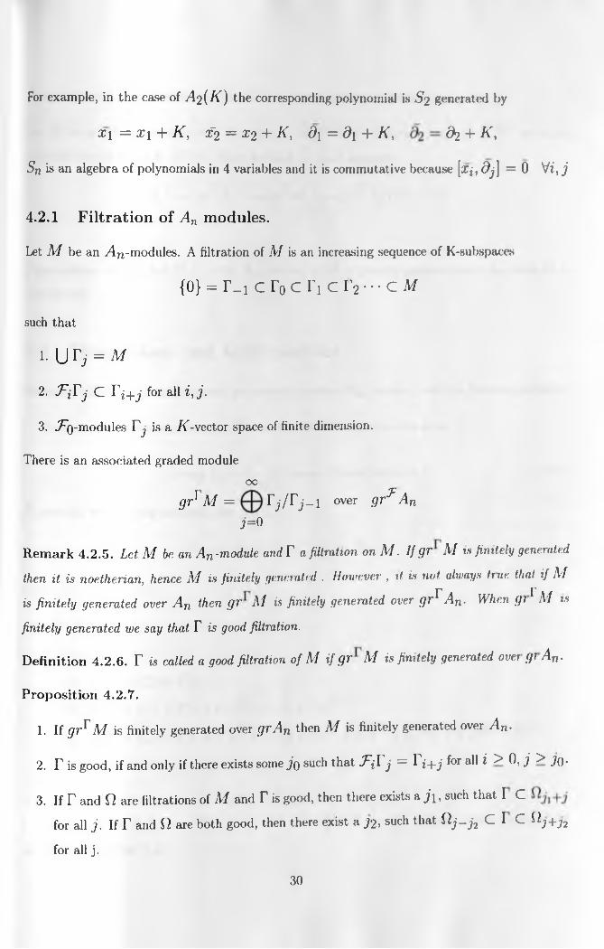
For example, in the case of ^ ( / F ) the corresponding polynomial is S 2 generated by

XI = x\ + K, £2 = X2 + K, d\=d\ + K, ^ + K,

Sn is an algebra o f polynomials in 4 variables and it is commutative because [ j j , dj] = 0 Vi, j

4.2.1 Filtration of An modules.

Let M be an y ln-modules. A filtration of M is an increasing sequence of K-subspaces

{0} = r_i c r0 c Ti c r2 • • • c m

such that

1 . U r j = M

2. FiTj C Yi+j for all i,j.

3. ,/~o_modules ^ is a /("-vector space of finite dimension.

There is an associated graded module

00

g r 1 M = T j / r j - 1 over g r ^ A n

3=0

R em ark 4.2.5. Let M be an An-module and Y a filtration on M. I f gr M is finitely generated

then it is noetherian, hence M is finitely generated . However , it is not always hue that if Mj . J1

is finitely generated over An then gr M is finitely generated over gr An- When gt l\f is

finitely generated we say that T is good filtration.

D efin ition 4.2.6. F is called a good filtration of M if gr A/ is finitely generated over gt An-

P ropos ition 4.2.7.

1. I f grrM is finitely generated over grAn then M is finitely generated over An-

2. r is good, if and only if there exists some j o such that T j Y j = F j+ j for all i > 0, j > Jo*

3. If T and Yt are filtrations of M and Y is good, then there exists a j\, such that I C

for all j . I f T and O are both good, then there exist a J2i such that t y - h C 1 C ^ J +32

for all j.

30

Proposition 4.2.8. Finitely generated A n-modules admit good filtrations.

Let M be a left A n module with filtration I\ Let N be a submodule, and set r ,1 n to be the

induced filtrations on N, M / N . Then we have an exact sequence

0 — ► gr N — * gr M — * gr1 M/N — ► 0

Proposition 4.2.9. Let M be a left A n module, if M is finitely generated over A n then M is

Noetheiian.

4.3 Dimensions and Multiplicities

Rem ark 4.3.1. From now onwards we restrict ourselves A n endowed with the B n stein filtration.

Consider the Bernstein filtration B j on A n . For this filtration we have

j 2nd im v B j = + terms of lower order in j (4.2)

J 2 n!To see this we take the simplest case i4 i((C )

B - i C B 0 C B x C B 2 C B 3 C - “

where B j are given as,

B -1 = {0 } ,

B0 =C1,B\ =C1 -j- Cx + Cd,

B2 =C1 + Cx + Cd + Cx2 + Cxd + Cd2B-i =C1 + Cx + Cd + Cx2 + Cxd + Cd2 + Cx3 + Cx2d + Cxd2 + Cd2

e.t.c

Now we consider the map j i----► d ifT lQ ( B j ); that is

1 .— » 3,2 .— ► 6,3 .— »10, - * - • — >• (j+1)jF+i l = h1 + lower order terms in j 85

claimed in equation (4.2)

31

Definition 4.3.2 (Hilbert polynomial). Let M be a finitely generated A n-module with a good

filtration { T j } , so that gr^ M is a finitely generated module over the graded nng S = g r1* An =

K[x l » -> Xm ^1) •••» dn\- Then, there exists a polynomial

x(M,r,t) = ^ t d + 0 ( td~1), m , d € Z +

such thatj

d im K T j = Y ^ d im x T j lT j . i = for j » 0

i=0This is the Hilbert polynomial of g rr M . Since grB An is a polynomial nng in 2n vanables,

d < 2n.

If T, Q are good filtration on M , by definition there exist a k such that:

x (M , Sl, j -k)<x{M, T , j ) < + *0

since the leading term of X is not affected by a shift in j . The numbers d = d(M) and

m = m ( M ) do not depend on the filtration T; d is called the dimension of the module M

while m is called the m ultip lic ity of M .

Example 4.3.3.

Let M = An and B be the Bernstein filtration. We want to find x ( A n,B, t ) , so we mad to

calculate the dim K ( B j ).Recall that B, is spanned by the monomials with M + <

so we want to find nonnegative solution to

m H-----an + Pi *4------ Pn < *•

The number of solutions is

( 2n - 1\ /

\2n - 1/ + \2n - 1/

So

/2n + i — 1\ _ f ^ n + *

" ' + V 2n - 1 ) ~ V 2n(i + 2n)(t + 2n — ! ) • • • ( * + 1)

2n!(t + 2n ) ( t + 2n - ! ) • • • ( * + 1)

0 = 2n!

2 n + l \

2n - 1/

32

This is a polynomial of degree 2Tl with leading coefficient l/(2n!). Thus d(An) = 2n and

m(An) = 1.

Example 4.3.4.

Let

M =An

= K [ x u - " , x n\^ = l A n dJ

and r be a standard filtration then d im (F j) = d = Tl andm = 1

Proposition 4.3.5. Let 0 ----> N ----» M --- > M /N --- ♦ 0 be an exact sequence of An-

modules with M a finitely generated A n-Tnodule and I a good filtration of M . Let l\ be a

submodule of M. Denote by and the filtration induced by I on N and A//N respectively.

Then

0 — > g r1'N — > g rl M — > gr1 M /N — * 0

is an exact sequence of gv^ An modules, T/ and I ,r are good fdtrations,and we have

i . x(M,r,o = x(M,r,,o + x(M,r",o

2. d ( M ) = rnax(d(N ) , d (M /N ) )

3. I f d ( N ) = d (M/N) then m { M ) = m{N ) + m {M / N )

Corollary 4.3.6. Let M = © f = i Mj be a direct sum of finitely generated A n modules.

Then d ( M ) = max(d(Mi ) ) . and if d (M) = d(Mi ) for 1 < i < k then m ( M ) —

E *= i

Corollary 4.3.7. If M is finitely An-module then d{M) £ 2Tl.

Proof. Since M is finitely generated implies there exists l elements which generates M and there

exists a surjection

A ln M — * 0

The theorem gives

d(Aln) =

On the other hand the previous corollary gives

d(A ln) = d(An) = 2 n

So d ( M ) < 2n.

33

We use the following technical lemma due to A. Joseph in the proof of Bernstein Inequality .

Lem m a 4.3.8. Let M be finitely generated An module with filtration Y with respect to B and

To ^ 0 . Then the K-linear map

Di — ♦ HomK (r j , r 2i ).

defined by sending a € Bj to the map U --- ► (LIL, is surjective

Proof. It is enough to show that aTj ^ {0 } whenever a 6 Bi is not 0. We proceed by induction

on i. For i = 0, Bq = K , so this follows from the fact that that Fq 7 0. Assume on the

contrary, aYi = {0} . We must have a (fc K, so a contains a term of the form ,with

|q | + \/3\ > 0. Suppose that some Ocj ^ 0. Then [a, dj] contains a terms OtjCXn eid^.\n

particular, it will be nonzero element of Z?z_i.We have

[a,dj ]Ti^i =ad jY i -\ +d jaYi -\ .

Since djYi—\ C Tz and aTz = 0, we have

[a ,dj ]Ti - i = 0 ,

which is a contradiction.

Similarly, suppose that some (3j ^ 0. Then contains a term (3jCXad‘ ( j . In particular

it will be a nonzero element of Z?z_ j. We have

[a,Xj]Yi-\ = ax j T i - i + xjaYi_\.

Since XjYi -\ C Tz and aTz = 0, we have

[a ,Z j ] IV i = 0 ,

which is also a contradiction.

T h eorem 4.3.9 (Bernstein Inequality 1971 [8| ). Let M ^ 0 be a finitely generated Aji-module.

Then d ( M ) > Tl.

Proof. We create a good filtration T of A/ by having a set of generators be in I q. So I q ^ 0.

The previous lemma then applies to give an injection

Bi — * HomK {Yi,Y2i)

34

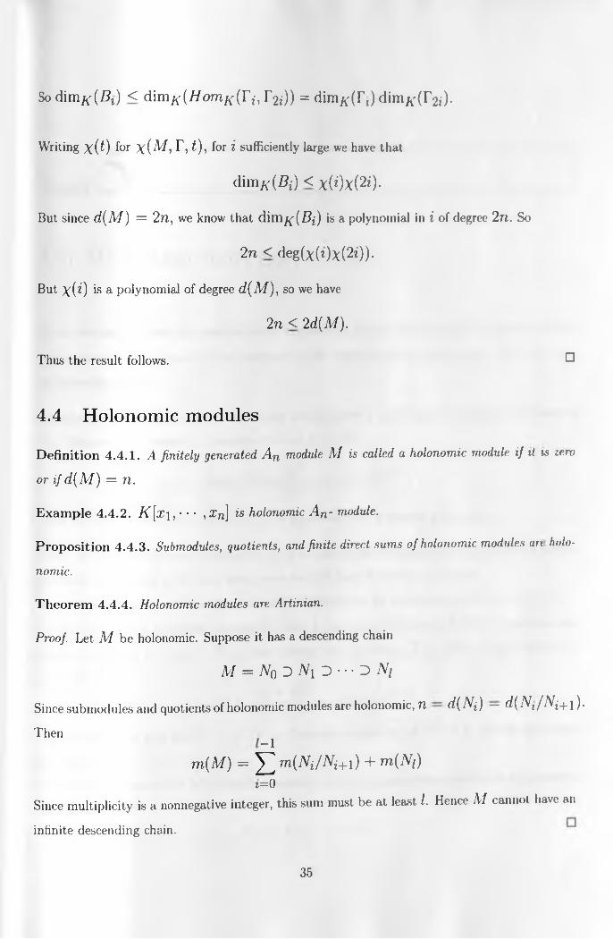
Writing \ { t ) for x(M, T, f ) , for i sufficiently large we have that

d im K (Bi) < x ( i ) x (2 i ) .

But since d (M ) = 2n, we know that d im k ( B i ) is a polynomial in i of degree? 2Tl. So

2n < d e g (x ( t )x (2 i ) ) .

But x(i) is a polynomial of degree d(M), so we have

2n < 2d(M).

Thus the result follows. ^

4.4 Holonomic modules

D efin ition 4.4.1. A finitely generated A n module M is called a holonomic module if it is zero

or if d (M ) = Tl.

E xam ple 4.4.2. K [ x \ , • • • , Xn\ is holonomic A n - module.

P ropos ition 4.4.3. Submodules, quotients, and finite direct sums of holonomic modules an holo­

nomic.

T h eorem 4.4.4. Holonomic modules are Artinian.

Proof. Let M be holonomic. Suppose it has a descending chain

M = iV0 D N\ D • • • D Ni

Since submodules and quotients of holonomic modules are holonomic, Tl d{ Ni ) — d( N t /N±+ ]).

Then-1

m(M) = ^ m(Ni/Ni+\) + m(N[)i=0

Since multiplicity is a nonnegative integer, this sum must be at least l. Hence M cannot have an

infinite descending chain.

So d im K {Bt) < d im /c(/ / om A' ( r j , r 2i ) ) = d im A- ( r , ) d im A' ( r 2i ) .

35

Chapter

The Bernstein-Sato polynomials

In this section we show the construction of a particular family of holonomic A n modules which

are necessarily for the proof of the existence of the Bernstein-Sato polynomials. First, we need

the following result.

L em m a 5.0.5. Let M be a left A n module with filtration T with respect to Berstein filtration of

A n . Suppose there exists C, C\ such that fo r all j > > 0,

d im # r j < c^—r T C\[ j + l ) ” - 1 .J n\

Then M is holonomic with m ( M ) < C. In particular, M is finitely generated.

Proof. We prove the lemma in two parts. First we show that the conclusion holds for every finitely

generated submodule of M , and then prove that M itself is finitely generated.

W e now show that every finitely generated submodule of M is holonomic with m ( M ) < C.

Let N be a finitely generated submodule. Then it has a good filtration Q. Thus there exists an

integer r with Q j C f l N , so that d i m < d im /^(rj-|-r ).B y our hypothesis, for

j » 0

x t i ) < c - +,r- + ci0 ' + d "-1-n\Hence d ( N ) < n and m ( N ) < C. By the Bernstein Inequality, d ( N ) = n. We are done with

the first part.

Now we want to prove that M is finitely generated. Choose an ascending chain of finitely generated

submodules of M

N\ C N2 C • • • C N [

36

Each is holonomic with 77l(iVj) < c. And since the iVt have the same dimension, their multiplic­

ities satisfy

So we have/

m ( M ) = m ( M ) + Y ' V n M / N i - 1)

i= 2

Since m ( N i ) < C and multiplicities are nonnegative integers, all ascending chains of finitely

generated submodules must have fewer than C steps. This implies that M must be finitely

generated.

We can thus apply the first part to M to see that it is holonomic with m ( M ) < C. □

R em ark 5.0.6. I f M is holonomic, then its length is bounded by m ( M ) and holonomic modules

are cyclic.

T h eo rem 5.0.7. Let p G K [ X ] . Then K [ X , p ~ ^ ] is a holonomic A n module.

Proof. Let m be the degree of p. We define a filtration V for K [ X , p 1 ], and show that this

filtration is amenable to an estimate as in the lemma. Set

r / = { f / p l : d eg (/ ) < ( m + 1 )1 }.

It is easy to check that all elements of K [ X , p '] are in some I /. It is similarly easy to see that

B,rt c r/+iand that the dimension of is bounded by the dimension of the space of polynomials of degree

< ( m 4- 1)/, so is finite dimensional. In particular, a similar counting trick as employed in the

proof that d ( A n ) = 2n shows that

d im k { ( tti + 1)/ + n ) • • • { { m + 1)/ + \)/n\.

Since the highest order term in l on the left hand side is (777. ~h 1) l /^*> there is a r sudi that

d im # T/ < c lu/n\.

We apply the lemma and are done.

37

The following example will illustrate:

Example 5.0.8. M = C[x,X is holonornic. A filtration I on M is given by T : Tq Cf i C r 2 C r 3 C • • • where

r 0 =C1

r i = c i + C x + C x ~1

r 2 =C1 + Cx 4- Cx’ 1 + Cx2 + Cx’ 2

r 3 =C1 4- Cx 4- Cx-1 + Cx2 4- Cx-2 4- Cx3 + Cx-3

Now the map j — > d im e T j ; 1 i— * 3,2 i— * 3 + 2,3 ■— * 3 4- 2 + 2

thus j ---- > 3 + 2 ( j — 1).

Let A be transcendental over K[X] = K[x\, - • • , Xn\. Consider the Weyl algebra An( K ( A ))

over /C(A); the field of rational functions in A. Let p € K[x\, • • • ,Xn} with deg(p) = m. W e define a symbol p^ on which the element d j acts by formal differentiation:

djpX = \p~ 1

So we define an An( K (A)) module M = K(X) [X, p~ ]p generated over K(X)[X,p~l}by

the generator Further let N = An(K(X)).p^ Introducing in M a filtration similar to the

one in Theorem 5.0.7 that is T j := { f - P ^ -P^\deg / < (m 4- l ) j } . Then M and N are

holonornic.

T h eo rem 5.0.9 (Generalisation of theorem 5.0.7). Let p G A " [X ], then K (A )[A f, p is a

holonornic A n [ K (A ) ) module. Hence its submodule A n (I\ (A ) ) p^ is also holonornic.

We need also the following result:

Lem m a 5.0.10. Now we have automorphism t of K (A ) [X , p ^]p^ defined by

*(aV ) = (a + i ) V

This is An(K) linear, but not AltK { A ) linear

38

5.1 Existence of Bernstein-Sato polynomial

We are now ready to prove that for every polynomial p G A [A"] there exists a corresponding a

Bernstein-Sato polynomial.

T h eo rem 5.1.1. Let p G K[x! , • • • , X n\, then there exist B ( A ) G A '[A ] and d (A ) G

A n ( K ) [ X ] such that

B{X)px = d(X)ppx (5.1)

Proof. Since An( K ( \ ) ) p ^ is holonomic, it is Artinian. Hence the descending chain

An(K(X))px D A n(K(X) )ppX A„(K(\) )p2px

must terminate. So there exist k such that

pkpX e A n ( K ( X )

We apply t~k to both sides, Noting that t ~ k (p kp X)is pX times a rational function in A we get

pX € A„(K(X))ppx

Clearing the denominators of A. we get that for some B( A) G A [A],

B(X) € A„(K)[X]ppx

So there is a d (A ) G An(K ) [A] with

B(X)px = d(X)PPx

Ar-h 1 _A

□

R em ark 5.1.2. This equation f5 .ll is called the B erns te in 's fu n c tio n a l equation. B ( A)

and d (A ) are not uniquely determined by this functional equation. However, by the fact that

the polynomial ring K [ A] is a principal ideal domain, there exists a unique polynomial b (A ) of

smallest possible degree which enters in a functional equation satisfied by a given polynomial p.

Here b {A ) is normalised so that its highest coefficient is 1 and b (A ) is called the. Bernstein-Sato

polynomial of p.

39

D efin ition 5.1.3. The B em s te in -S a to polynom ial o r b -fu n ction of p, written b (A ), is

defined to be the monic generator of the ideal of all possible B ( A) satvsfying the Bernstein’s

functional equation.

Exam ple 5.1.4. Let p ( x ) = X. Then

= (A + l ) x A ax

Hence b( A ) = A + 1 is the b-function o f p and d (A) = g j .

Exam ple 5.1.5. Let p ( x ) = X^ - f • • • + X„

Then

d ip {x )X+1 = 2 (A + l ) x j p ( x ) A

d f p ( x ) x+1 = 4A (A + l ) x ^ p (x )A_1 + 2 (A + l ) p ( x ) A

Hence d (A ) = ^ ! i = \ satisfies

d (A )p ( x )A+1 = 4A (A + l ) p ( x ) p ( x )A_1 + 2 n (A + l ) p ( x ) A

= 4 ( A + l ) ( A + ^ ) p ( x ) A

Thus

fe(A) = (A + l ) ( A + ^ )

is a b-function.

5.2 Solution of the Analytic Continuation Problem

Let ( p{x) G C ™ ( R n ) - a test function on R n. Consider a polynomial p = p [ x i , • • • , Xn] £

R [ x j , • • • , x n ] with nonnegative values on R 7* and let A G C , R e A > 0 then ] ) as a coni inuous

function in R 7? thus it makes sense as a distribution on R .

40

In fact, we define

^ ( A ) = / p ( x )X<t>(x)dx (5.2)J R n

Then r ^ (A ) G T>r and A ---- * r ^ (A ) is holomorphic family on {A G C|7£eA > 0 }

C oro lla ry 5.2.1. Let I ^ (A ) G has a meromorphic extension to all of C with poles in

{A|6(A + j ) = 0 } fo r some j G N.

Proof. From

D { X ) p X = d (\ )p x+1

By partial integration

r ^ (A ) j d (\ )p X+1<j>(x)dx

= b (\ ) J P X + ld {\ )4 > {x )d x

= b & b { ^ J p X + 2 d { X + 1 ) d { m

1 1

6 (A )6 (A + 1)

1p x+ N d ( A + N

b (\ + N - l ) j1) ■ • • d(A + l)d(\)<t>(x)dx

By taking N very large, we see that [ ^ (A ) is merornorphically continued to the whole space

A G C and that its poles are contained in { a j - k , j = 1, • • • , 771, k = 0 ,1 ,2 , • • • } where

Ckj is any root of 6 (A ). E

41

5.3 Conclusion

In this report, we have seen the treatment of purely analytic problem by algebraic means. This

gives a beautiful and easy to follow solution compared to its analytic flavoured solution. This is

exactly one of the reasons why we ought to study D-inodule theory. Generally, numerous results

can be reformulated and proved in this manner.

The theory of algebraic D-inodules was developed to provide an algebraic study of partial dif­

ferential equation. In fact, as a motivation for the theory, we explained in chapter 1 how to make

the switch from the usual point of view of systems of partial differential equations to the point of

view of D-modules.

Most importantly, the theory of algebraic D-modules, becomes very interesting if one is familiar

with basic knowledge of linear algebra, homological algebra, sheaf theory and analytic geometry;

that is algebraic geometry and linear symplectic geometry; for instance, it is not easy to give a

geometrical interpretation of the dimension of ^4^-module, if one is not conversant with the lan­

guage of algebraic geometry and linear symplectic geometry. Accordingly, using D-modules one

could reformulate the famous Cauchy-Kovalevskaya theorem;on the existence and uniqueness of a

local solution and prove it in a purely algebraic form after introducing the characteristic variety

o f a system. See the proof in [20|.

Finally, we will wish to point out that the theory of D-modules, which is now often referred

as "Algebraic Analysis", has grown steadily during the past years and important applications to

other fields of mathematics and physics (e.g. singularities theory, group representat ions, Feynman

integrals, e.t.c ) were developed. Therefore, the task facing a student who would like to work in

these directions is quite impressive: the research literature is huge and many research areas aie

still open.

42

Bibliography

[1] S.C.Coutinho: A primer of algebraic D-modules, Cambridge University Press. 42, (1995)

[2] Gunter R. Krause and Thomas H. Lenagan, Growth of algebras and Gelfand- K irillov dimen­

sion, revised ed.,Graduate Studies in Mathematics, vol. 22, American Mathematical Society,

Providence, RI, 2000.

[3] D.H. Griffel: Applied Functional Analysis, Mathematics and Application Ellis Horwood Se-

ries.42, (1981)

[4] J.E Bjork: Rings of Differential Operators,Mathematical Library vol. 21 Amsterdam, (1979)

[5] Robert S. Schrichartz: A guide to Distribution Theory and Fourier Transforms, Studies in

Advanced Mathematics, CRC Press.42. (1994)

|6] I. N. Bernstein:Modules over a ring o f differential operators. An investigation o f tin funda­

mental solutions of equations with constant coefficients,,Funkcional. Anal, i Prilozen. •> (1971),

no.2, 1-16.

[7| I. N. Bernstein and S. I. Gelfand: Meromorphy of the function P , Funtioonal. Anal, i

Prilozen. 3 (1969), no. 1,84-85.

[8] I. N. Bernstein \The analytic continuation of generalised functions with parameter, Fun-

tional.Anal. and Appl. vol.6 (1972), no.4,26-40

[9] Masaki Kashi warn: B-functions and holonomic systems. Rationality o f roots o f b- functions,

Invent. Math. 38 (1976/77), no. 1, 33U53. MR MR0430304 (55 #3309)

[10] I.M. Gelfand and G.E. Shilov:Generalised functions. Vol.l, Academic Press, New York 1964.

43

111] M.F. Atiyah:Resolution o f singularities and division of distributions Coimn. Pure and App.

Mathematics 23,1970.

[12] Anton Leykin.Introduction to the algorithmic D-module theory Institute for Mathematics and

its Applications,August 2006.

113] M. Kashiwara: D-modu/es and microlocal Calculus translated from 2000 Japanesse original

by Mutsumi Saito. Translation of Mathematic Monographs, 217, Iwanami Series of Modern

Mathematics, AMS, Providence, RI,2003.

[14] Malcolm A. H. Maccallum and Alexander V. Mikhaillov:AIgebraic Theory of Differential

Equations., London Mathematical Society Lecture Note Series: 357, Cambridge University

Press, 2009

[15] Santanu ChakrabortyiiSorae Applications of Dirac’s Delta Function in Statistics fo r More

Than One Random Variable., Applications and Applied Mathematics: Vol. 3, No. 1 (June

2008) pp. 42-54

[16] Walter Rudin:Functional Analysis., McGraw-Hill, Inc,. 1973.

[17] Ruel V. Churchill,James W. Brown and Roger F. Verhey.Complex Variable and Applications.,

McGraw-Hill, Inc,. 1976.

|18] Ricardo Estrada and Ram P. Kanwal :A Distributional Theory fo r Asymptotics Theory and

Applications., Birkhauser Boston, 2002.

[19] William R. Wade .An Introduction to Analysis. Prentice Hall, New Jersey 1995.

[20] Masaki Kashiwara : Algebraic study of systems of paiiial differential equations. Master I hesis,

Tokyo University, December 1970. Translation by Andrea D ’Agnolo and Jean-Pierre Schnei­

ders, Memoires 65 de la S.M.F, 1995.

44

Index

analytic continuation, 4

Artinian, 39

associated graded module, 30

automorphism, 38

b-function, 40

Bernstein Inequality, 34

Bernstein polynomial, 22

Berstein filtration, 31

continuation of distributions, 20

continuously differentiable, 12

d'Alembert, 10

D-module Theory, 26

degree of operator, 27

Derivative of a distribution, 17

dimensions, 31

Dirac delta function, 6

filtrations, 28

finitely generated, 30

functional, 14

Heisenberg relations, 26

Hilbert polynomial, 32

holomorphic family, 22

holonomic modules, 35

induced filtrations, 31

Lebesgue integral, 15

meromorphically, 22

multiplicities, 31

noncommutative ring, 27

open sets, 3

Poincare-Birkhoff- Witt, 27

rational function, 39

Sato, 22

support of a function, 12

test function, 12

topology, 3

Weyl Algebra, 26

good filtration, 30

grading, 28

Heaviside step-function, 8

45