The Alaskan pipeline, a significant accomplishment of the engineering profession, transports oil...
21
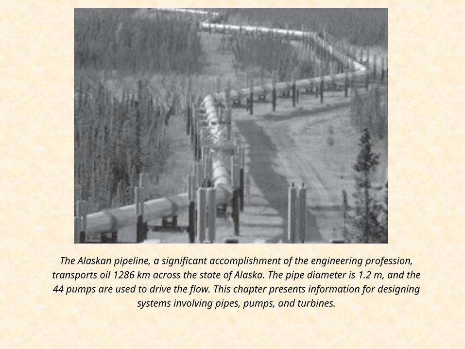
The Alaskan pipeline, a significant accomplishment of the engineering profession, transports oil 1286 km across the state of Alaska. The pipe diameter is 1.2 m, and the 44 pumps are used to drive the flow. This chapter presents information for designing systems involving pipes, pumps, and turbines.
-
Upload
hester-montgomery -
Category
Documents
-
view
215 -
download
1
Transcript of The Alaskan pipeline, a significant accomplishment of the engineering profession, transports oil...
The Alaskan pipeline, a significant accomplishment of the engineering profession,transports oil 1286 km across the state of Alaska. The pipe diameter is 1.2 m, and the44 pumps are used to drive the flow. This chapter presents information for designing
systems involving pipes, pumps, and turbines.

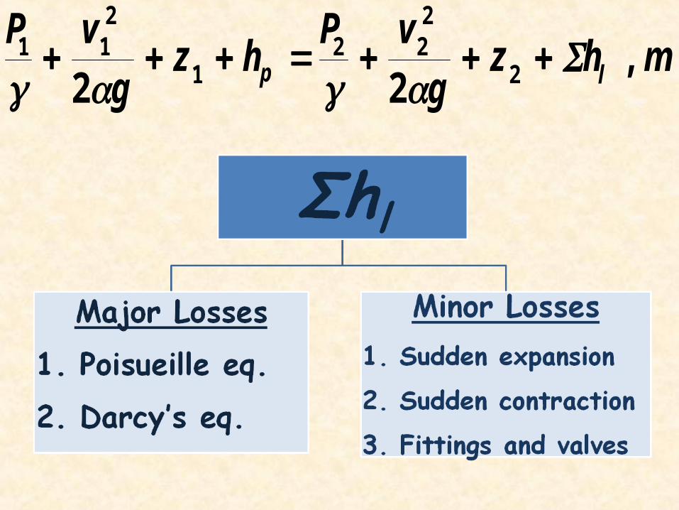
Typical Applications· For flow in a pipe, find the pressure drop
or head loss.· For a specified system, find the flow
rate.· For a specified flow rate and pressure
drop, determine the size of pipe required.
· For a system with a pump, find the pump specifications (power, head, flow rate).
· For a specified elevation change and flow rate, find the power that can be produced by a turbine.

1.Development of Pipe Correlation
1.1 Analytical Approach

Viscous Flow in Pipes
m hzg
vPhz
gvP
lp ,22 2
222
1
211

Pressure Drop in Laminar Flow
The forces on it are: 1- pδA in flow direction 2- p’δA on the reverse direction. 3- friction force acting on its outer-surface. (on the reverse direction of flow)

1.1.1 Force Balance on the Element
2
2
02
r Ad : since
rdl dldAlp
or
(1) .................. )rdl (dA)dllp
p(pdA
And assume (p) changes with (l) only
.
dldp
lp
.,e.i
(2) ................... r
.dldp
2

(5) ..................... dr]dldp
[r
dv
(4) .................... ]dldp
[r
drdv
(3) ................... r
.dldp
drdv
2
2
2
(6) ............ constantr
]dldp
[v
4
2
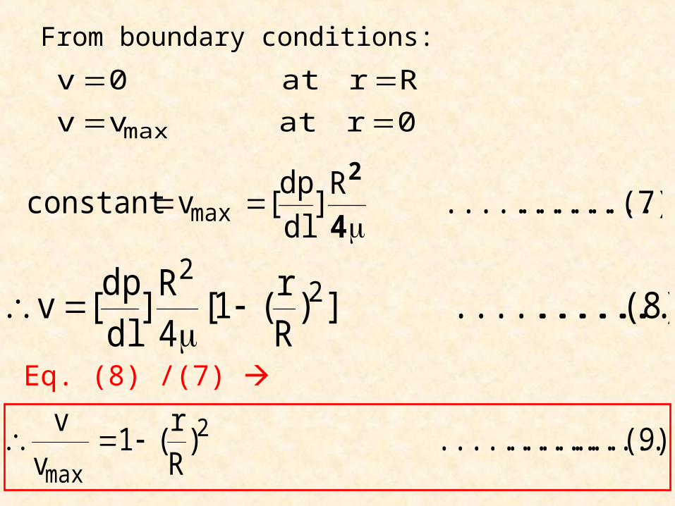
From boundary conditions:
0r at vv
Rr at 0v
max
(7) .................... R
]dldp
[vconstant max
4
2
(8) .................... ])Rr
(1[4R
]dldp
[v 22
(9) ....................... )Rr
(1v
v 2
max
Eq. (8) /(7)
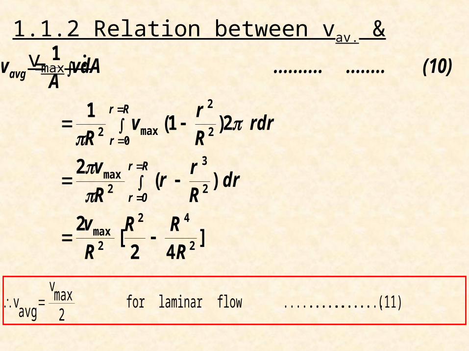
1.1.2 Relation between vav. & vmax :
]42
[2
)(2
2)1(1
1
2
42
2max
2
3
2max
02
2
max2
RRR
Rv
dr Rr
rRv
rdr Rr
vR
(10) .................. vdAA
v
Rr
0r
Rr
r
avg
(11) ............................ flow laminar for 2
maxv avgv

From (7) in (11)
(13) ................... Poiseuille - Hagen D
vl32p 2
(7) .................... R
]dldp
[vconstant max
4
2
(12) .............. pipe of diameter inside 2R D ; 32D
]dldp
[v2
avg
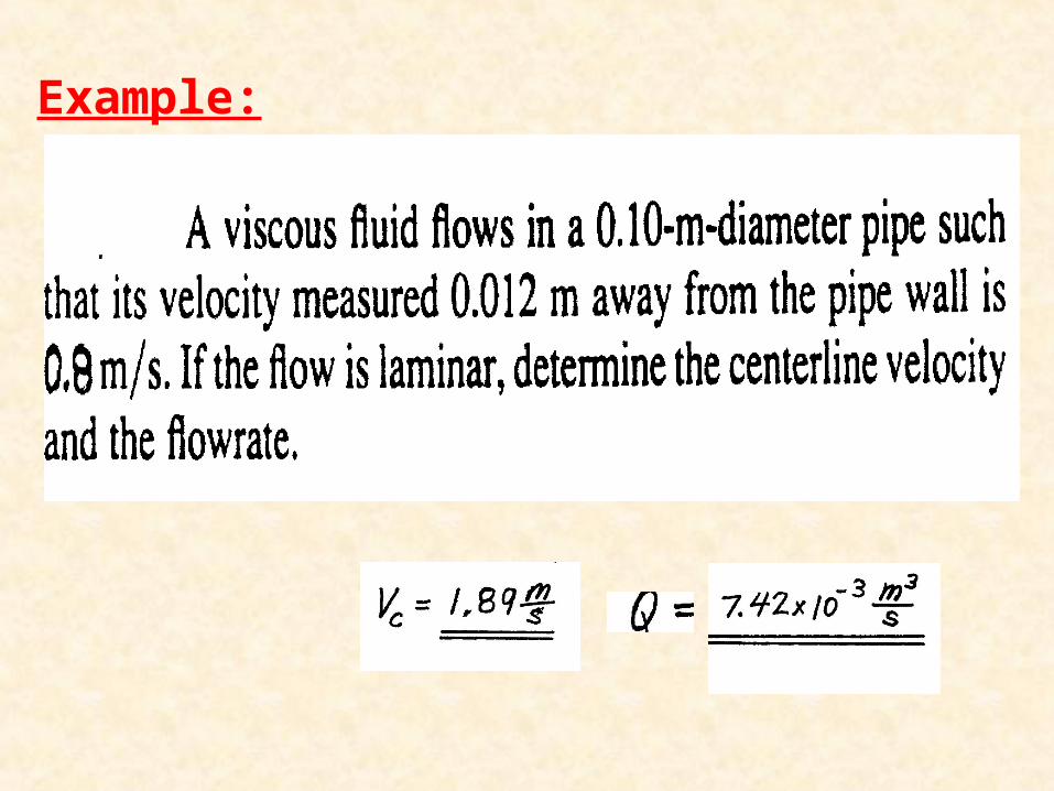
Example:

1.1.3 Use of friction factor (f) for friction losses determination
(14) ,........ N/m , D2Lvf4
P
2v
surface theat stressshear
2/v RL2
R.P
v21 times )( density of product
areaunit surface wettedforce) tionforce(fric drag
f
22
f
2
2
2
2
equation Weisbach -Darcy

(16) ........ Re64
f & Re16
f
factor friction Moody'ff4 ; Re64
'f
Re64
f4
(15) ................... D2Lvf4
DvL32
Moodyfanning
2
2
•For laminar flow sub. ΔPf by Hagen-Poiseuille in Darcy’s eq. :
•For turbulent flow f = φ( Re, ϵ) ; ϵ is roughness factor•f is predicted from Moody diagram or fanning diagram
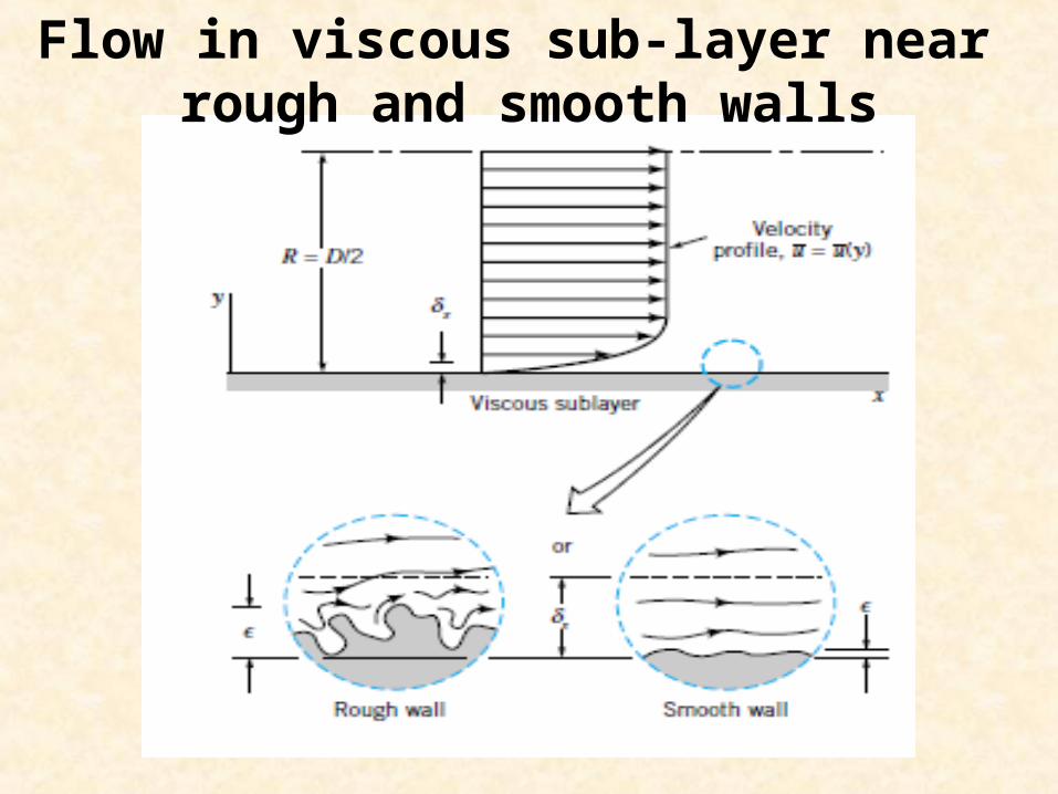
Flow in viscous sub-layer near rough and smooth walls


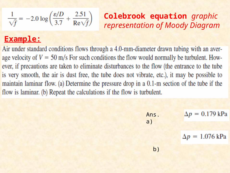
Colebrook equation graphic representation of Moody DiagramExample:
Ans. a)
b)

Example:

Example:


![[WIR-1286]868MHz LORA Wireless Module - …robokits.download/datasheets/WIR_1286.pdf · [WIR-1286]868MHz LORA Wireless Module Page 1 LORA 868MHz Wireless serial link [WIR-1286] Contents](https://static.fdocuments.us/doc/165x107/5b8250287f8b9aad638e4423/wir-1286868mhz-lora-wireless-module-wir-1286868mhz-lora-wireless-module.jpg)