The Air Traffic Flow Management Problem withEnroute Capacities

Dimitris BertsimasSarah Stock

WP# - 3726-94 MSA August, 1994

The air traffic flow management problem with enroute capacities

Dimitris Bertsimas 1 Sarah Stock 2 3

August 1994

1 Dimitris Bertsimas, Sloan School of Management and Operations Research Center, MIT, Cam-

bridge, MA 02139.2 Sarah Stock, Operations Research Center, MIT, Cambridge, MA 02139.3 Research supported in part by grants from Draper Laboratory and the FAA and by a Presidential

Young Investigator Award DDM-9158118.

Abstract

Throughout the United States and Europe, demand for airport use has been increasing rapidly

during recent years, while airport capacity has been stagnating. Acute congestion in many

major airports has been the unfortunate result. For U.S. airlines, the total yearly delay costs

resulting from congestion are estimated to be on the order of $2 billion, while the total losses

of all U.S. airlines amounted to approximately $2 billion in 1991 and $2.5 billion in 1990.

European airlines are in a similar plight. Optimally controlling the flow of aircraft either

by adjusting their release times into the network (ground-holding) or their speed once they

are airborne is a cost effective method to reduce the impact of congestion on the air traffic

system. Current models addressing this problem assume that the only capacitated elements

in the system are the airports. The contribution of this paper is twofold: a) We build a model

that takes into account the capacities of the National Airspace System (NAS) as well as the

capacities at the airports and extend that model to account for several variations of the basic

problem, most notably, how to reroute flights and how to handle banks in the hub and spoke

system. b) We solve large scale, realistic size problems with several thousand flights, improving

significantly on the state of the art.

1 Introduction

Throughout the United States and Europe, demand for airport use has been increasing rapidly

during recent years, while airport capacity has been stagnating. Acute congestion in many

major airports has been the unfortunate result. For U.S. airlines, the total yearly delay costs

resulting from congestion are estimated to be on the order of $2 billion. In order to put this

number in perspective, the total reported losses of all U.S. airlines amounted to approximately

$2 billion in 1991 and $2.5 billion in 1990. European airlines are in a similar plight. Thus,

congestion is a problem of undeniable practical significance. Not only is the congestion problem

severe, but it is also expected to get worse. The Federal Aviation Administration (FAA)

predicts a 25% increase in demand for airport operations by the year 2000, while no appreciable

increase in capacity is expected.

Faced with the realities of congestion, the FAA has been using ground-holding policies to

reduce delay costs. These short-term policies consider airport capacities and flight schedules

as fixed for a given time period, and adjust the flow of aircraft on a real-time basis by imposing

"ground holds" on certain flights. Such a flight is then held on the ground at its departure

airport even if it is otherwise ready for take-off. Ground-holding makes sense in the following

situation. Suppose it has been determined that if an aircraft departs on time, then it will en-

counter congestion, incurring an airborne delay as it awaits landing clearance at its destination

airport. However, by delaying its departure, the aircraft will arrive at its destination at a later

time when minimal congestion is expected, thus, incurring no airborne delay. Therefore, the

objective of ground-holding policies is to "translate" anticipated airborne delays to the ground.

The effectiveness of ground-holding policies lies in the following two fundamental facts.

First, while a flight is airborne it incurs costs such as fuel and safety costs that are not

applicable before the flight takes off. These costs make airborne delays much costlier than

ground delays. Second, airport capacity is highly variable due to its heavy dependence on

the weather (visibility, wind, precipitation, cloud ceiling). It is not unusual for the capacity

of an airport to be reduced by 50% in inclement weather. Given these two facts, there is

significant potential to reduce costs when adjusting aircraft flow as weather (hence airport

capacity) forecasts change in such a way that ground delays are substituted for the much

1

costlier airborne delays. Currently, the FAA implements a national ground-holding policy.

However, the selection of appropriate ground-holds is based on the experience of its air traffic

controllers rather than on a formal optimization model.

A Taxonomy of Problems

In Odoni (1987), the problem of scheduling flights in real-time in order to minimize congestion

costs was first conceptualized and introduced. Since then several models have been proposed

for solving different versions of this problem. The first and simplest version only considers

a single airport and makes decisions about the ground-holds for this Single-Airport Problem

(SAGHP). The Multi-Airport Ground-Holding Problem (MAGHP) was the next problem to

be introduced. It only makes ground-holding decisions, but considers an entire network of

airports. Thus, the SAGHP and the MAGHP are distinguished by whether delays are assumed

to propagate in the network as aircraft perform consecutive flights. Besides determining release

times for aircraft (ground-holding), the Air Traffic Flow Management Problem (TFMP) also

determines the optimal speed adjustment of aircraft while airborne for a network of airports

taking into account the capacitated airspace. Thus, the TFMP determines how to control a

flight throughout its duration, not simply before its departure. If we add the final complication,

rerouting of flights due to drastic fluctuations in the available capacity of airspace regions, we

obtain the Air Traffic Flow Management Rerouting Problem (TFMRP). In this problem, a

flight may be rerouted through a different flight path in order to reach its destination if the

current route passes through a region that is unusable for reasons usually related to poor

weather conditions. In order to describe the work on these problems we consider the following

modeling variations:

1. Deterministic vs. stochastic models, which are distinguished by whether the capacities of

the capacitated elements in the system (airports and sectors in the airspace) are assumed

to be deterministic or random.

2. Static vs. dynamic models, which are distinguished by whether or not the solutions are

updated dynamically during the day.

The deterministic SAGHP (both static and dynamic) was first formulated as a network flow

problem in Terrab and Odoni (1991). The stochastic SAGHP was formulated and solved as a

2

stochastic programming problem in Richetta and Odoni (1992) (the static case) and Richetta

and Odoni (1992) (the dynamic case). A review of optimization models for the SAGHP is

given in Andreatta, Odoni and Richetta (1993). The deterministic MAGHP was formulated as

a 0-1 integer programming problem in Vranas, Bertsimas and Odoni (1994a) (the static case)

and in Vranas, Bertsimas and Odoni (1994b) (the dynamic case). Terrab and Paulose (1993)

address the stochastic MAGHP as a stochastic programming problem.

All the previous work assumes that the only capacitated elements in the system are airports.

In this paper we present 0-1 integer programming models for the deterministic, multi-airport

TFMP which addresses capacity restrictions on the en route airspace and for the (TFMRP)

which addresses the rerouting of flights (TFMRP). Helme (1994) has presented a method for

the TFMP by designing a multicommodity minimum cost flow model over a network in space-

time. So far this method has not been tested, but it is expected that there will be severe

dimensionality problems. Lindsay, Boyd and Burlington (1993) propose integer programming

formulations for a version of TFMP that tracks a flight as it passes from fix to fix in the

airspace. As the linear programming relaxations of these formulations are not very strong,

branch and bound is needed to generate integral solutions, which increases the computation

times considerably. The TFMRP has not previously been addressed. In this paper, we present

a 0-1 integer programming formulation of the TFMRP.

Contribution of this work

Apart from extending all previous work on the ground-holding problem, we feel that our work

makes the following contributions:

1. In the last fifteen years the field of polyhedral combinatorics has demonstrated that the

key to solving large scale integer programming problems is to obtain strong formula-

tions, which include facets of the convex hull of solutions. Our success in solving large

scale, practical size instances of the TFMP lies exactly on this principle. We propose an

integer programming model for the TFMP which is rather strong as some of the proposed

inequalities are facet defining for the convex hull of solutions.

2. We address the complexity of the TFMP and show that it is NP-hard.

3

3. The solutions of the LP relaxation of the TFMP were almost always integral, so there was

no need to branch and bound. As a result, the computation times were reasonably small

for large scale, realistic size problems involving thousands of flights. This significantly

improves the state of the art in solving this class of problems. Short computational times

and integrality properties are particularly important, since these models are intended to

be used on-line and solved repeatedly during a day.

4. When specialized for the MAGHP, we prove that the LP relaxation bound of our for-

mulation is stronger when compared to all others proposed in the literature. As our

model gives solutions that were almost always integral experimentally, there is no need

for rounding heuristics that were used in Vranas et. al. (1994a).

5. We illustrate how our models can be adjusted to account for several variations in the

problem's characteristics, most notably how to handle banks in the hub and spoke system

and how to reroute flights (the TFMRP problem).

The paper is structured as follows. In Section 2 we formally introduce the TFMP and

present our formulation. In Section 3 we address the complexity of the TFMP. In Section 4

we address modeling variations for the TMFP including our formulation for the TFMRP. In

Section 5 we examine the theoretical properties of our formulation proving that the proposed

constraints are facet defining providing insights on the excellent computational performance.

In Section 6 we report computational results and in Section 7 we include some concluding

remarks. We include some technical proofs in the appendices.

2 The Air Traffic Flow Management Formulation

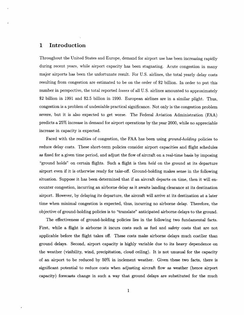
The National Airspace System (NAS) is divided into sectors. A map of the United States that

displays all of the sector boundaries is given in Figure 1. Each flight passes through contiguous

sectors while it is en route to its destination. There is a restriction on the number of airplanes

that may fly within a sector at a given time. This number is dependent on the number of

aircraft that an air traffic controller can manage at one time, the geographic location and the

weather conditions. We will refer to the restrictions on the number of aircraft in a given sector

4

at a given time as the en route sector capacities. There are several key sectors throughout the

United States that are often operated at full capacity. The issue of congestion at these sectors

is as critical as congestion in the terminal areas, since the cost of holding an airborne aircraft

is not dependent on the location of the aircraft. Thus, airborne delay costs could further be

reduced if we could determine the optimal time for a flight to traverse the capacitated sectors.

We first formulate the TMFP, examine the size of the formulation and make the connection

with the ground-holding problem.

2.1 The 0-1 IP Formulation

Consider a set of flights, F = {1, ... ,F}, a set of airports, KC = 1, ... ,K}, a set of time periods,

T = 1, ... ,T}, and a set of pairs of flights that are continued, C = (f', f) : f' is continued

by flight f}. We shall refer to any particular time period t as the "time t." The problem input

data are given as follows:

Data:

Nf = number of sectors in flight f's path

P(f, i) = the ith sector in flight f's path

Pf = (P(f,i): 1 < i < N)

Dk(t) = departure capacity of airport k at time t

Ak (t) = arrival capacity of airport k at time t

Sj (t) = capacity of sector j at time t

df = scheduled departure time of flight f

rf = scheduled arrival time of flight f

Sf = turnaround time of an airplane after flight f

C9f = cost of holding flight f on the ground for one unit of time

ca- = cost of holding flight f in the air for one unit of time

Ifj = number of time units that flight f must spend in sector j

T = set of feasible times for flight f to be in sector j

5

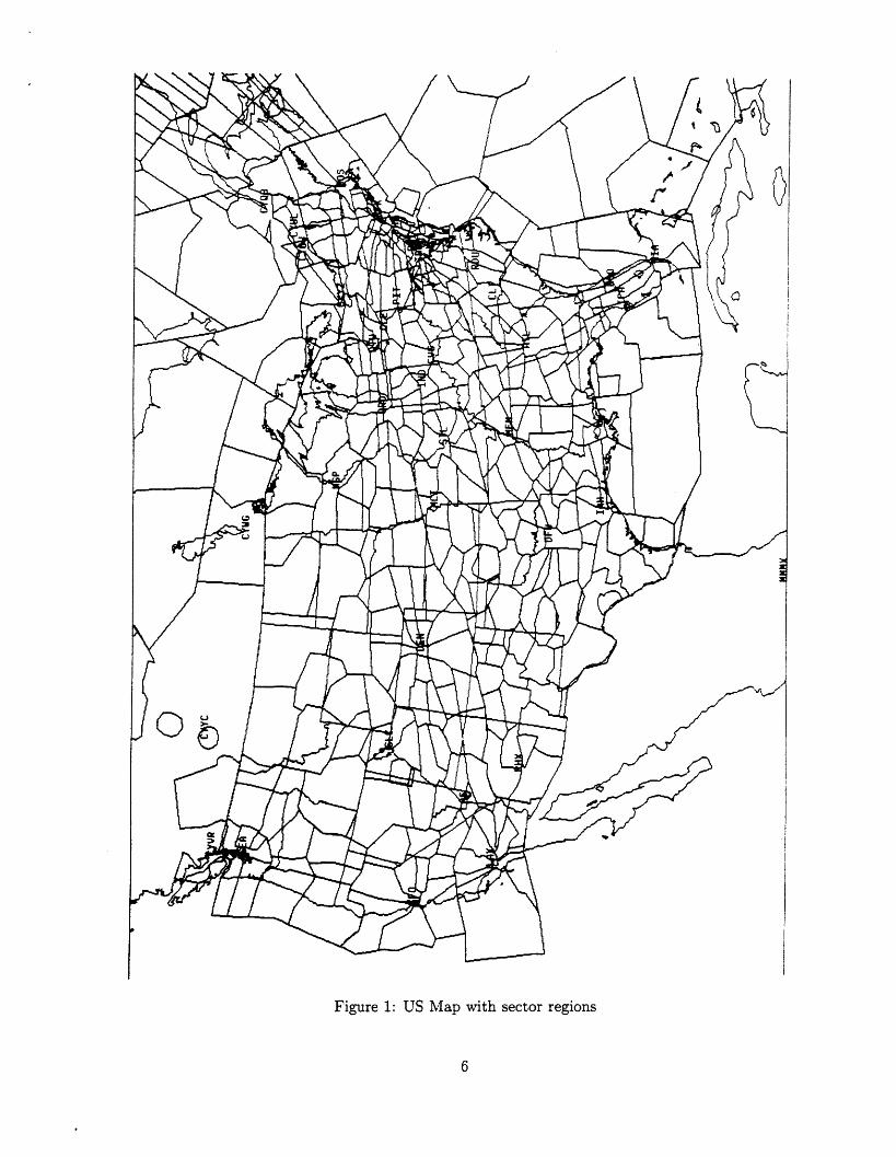
Figure 1: US Map with sector regions

6

0 -

Note that by "flight", we mean a "flight leg" between two airports. Also, flights referred

to as "continued" are those flights whose aircraft is scheduled to perform a later flight within

some time interval of its scheduled arrival.

Objective: The objective in the TFMP is to decide how much each flight is going to be held

on the ground and in the air in order to minimize the total delay cost.

We model the problem as follows:

Decision variables:

- 1 if flight f arrives at sector j by time t

fit - to0 otherwise.

Note that the wft are defined as being 1 if flight f arrives at sector j by time t. This definition

using by and not at is critical to the understanding of the formulation. Also recall that we have

also defined for each flight a list Pf of sectors which includes the departure and arrival airports,

so that the variable Wuft will only be defined for those sectors j in the list Pf. Moreover, we

have defined T] as the set of feasible times for flight f to be in sector j, so that the variable wft

will only be defined for those times within TJ. Thus, in the formulation whenever the variable

wft is used, it is assumed that this is a feasible (f, j, t) combination. Furthermore, one variable

per flight-sector pair can be eliminated from the formulation by setting wi/Tf = 1 where Tfj

is the last time period in the set T . Since flight f has to arrive at sector j by the last possible

time in its time window, we can simply set it equal to one as a parameter before solving the

problem. To ensure the clarity of the model, consider the following example which depicts two

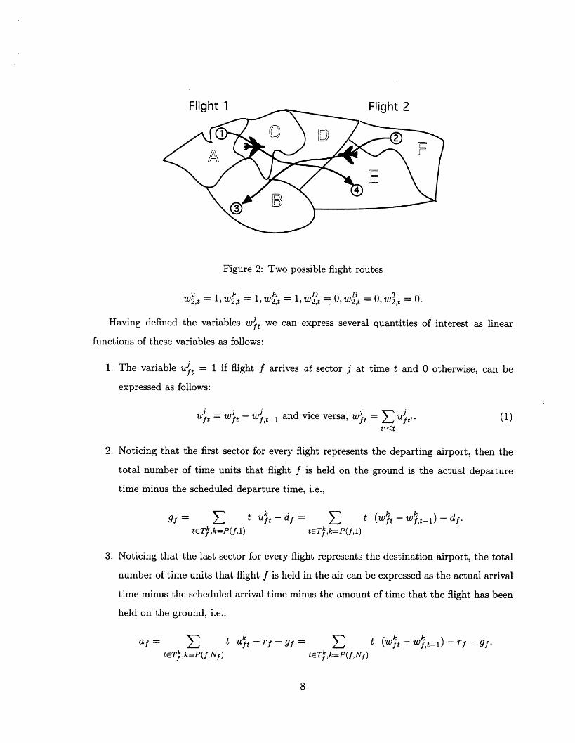
flights traversing a set of sectors. See Figure 2.

In this example, there are two flights, 1 and 2, each with the following associated data:

P1 = (1, A, C, D, E, 4) and P2 = (2, F, E, D, B, 3).

If we consider the current position of the aircraft to occur at time t, then the variables for

these flights at this time will be:

Wt = 1, Wt = 1, t 1 , w ,W = , W4t = , and

7

Ilinht 1 Flinht

Figure 2: Two possible flight routes

W2,t = , 2,t= , 2,t = , 2 t = O , w 2, t = O , W 2t = .

Having defined the variables wft we can express several quantities of interest as linear

functions of these variables as follows:

1. The variable u ft = 1 if flight f arrives at sector j at time t and 0 otherwise, can be

expressed as follows:

ft = t - Wf,t- and vice versa, W3ft = E uft, (t'<t

2. Noticing that the first sector for every flight represents the departing airport, then the

total number of time units that flight f is held on the ground is the actual departure

time minus the scheduled departure time, i.e.,

gf = E t u -df = E t (Wt Wt--l) - df.tETfk,k=P(f, l1) tETfk,k=P( f ,1)

3. Noticing that the last sector for every flight represents the destination airport, the total

number of time units that flight f is held in the air can be expressed as the actual arrival

time minus the scheduled arrival time minus the amount of time that the flight has been

held on the ground, i.e.,

af = t uft-rf -gf =t (wt --fW,t_1) - rf - gf

tETk,k=P(f,Nf) tETf,k=P(f,Nf )

8

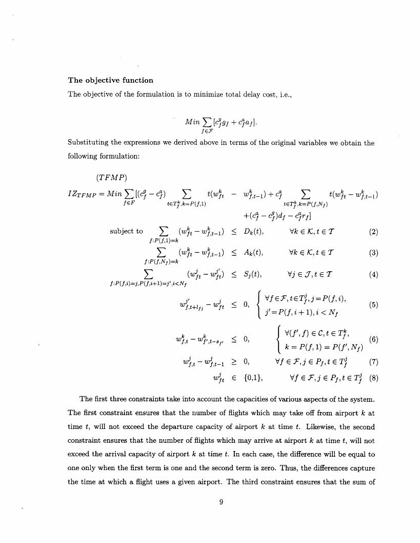
The objective function

The objective of the formulation is to minimize total delay cost, i.e.,

Min Z [ fgf + cfaf].fE-F

Substituting the expressions we derived above in terms of the original variables we obtain the

following formulation:

(TFMP)

IZTFMP = Min E [(C9f- Ca) ZfEF tETfk,k=P(f,1)

subject to E (wt - ,t_)f:P(f,l)=k

Z (Wt - Wk,t-1)f:P(f,Nf)=k

E (wft - wft)f:P(f,i)=j,P(f,i+l)=j',i<Nf

Wf,t+lf- Wft

k kWf,t WfI,tsf

ft -f,t-1l

WItft

- Wtl)+Caf ZtETfk,k=P(f,Nf)

+(c - cgf)df - carf]

< Dk(t), lVk E C,t E

< Ak(t), ¥k E C, t E'

< Sj(t, VjE, t E ,

< 0, Vf E F, tETf, j =Pi

, j'=P(f,i+ 1),i <

< 0,

> 0,

E 0,1},

The first three constraints take into account the capacities of various aspects of the system.

The first constraint ensures that the number of flights which may take off from airport k at

time t, will not exceed the departure capacity of airport k at time t. Likewise, the second

constraint ensures that the number of flights which may arrive at airport k at time t, will not

exceed the arrival capacity of airport k at time t. In each case, the difference will be equal to

one only when the first term is one and the second term is zero. Thus, the differences capture

the time at which a flight uses a given airport. The third constraint ensures that the sum of

9

t(Wt - Wt-1)

T

r

(f,i),

Nf

(2)

(3)

(4)

(5)

(6)

(7)

(8)

V(f',f)E C,t E T,

k = P(f, 1) = P(f', Nf)

Vf E , j E P , t E T]

Vf e F,j E Pf,t e T

all flights which may feasibly be in sector j at time t will not exceed the capacity of sector j

at time t. This difference gives the flights which are in sector j at time t, since the first term

will be 1 if flight f has arrived in sector j by time t and the second term will be 1 if flight f

has arrived at the next sector by time t. So the only flights which will contribute a value 1 to

this sum are the flights that have arrived at j and not yet departed by time t.

Constraints (5) represent connectivity between sectors. They stipulate that if a flight

arrives at sector j' by time t + Ifj, then it must have arrived at sector j by time t where j

and j' are contiguous sectors in flight f's path. In other words, a flight cannot enter the next

sector on its path until it has spent fj time units (the minimum possible) traveling through

sector j, the current sector in its path.

Constraints (6) represent connectivity between airports. They handle the cases in which a

flight is continued, i.e., the flight's aircraft is scheduled to perform a later flight within some

time interval. We will call the first flight f' and the following flight f. Constraints (6) state

that if flight f departs from airport k by time t, then flight f' must have arrived at airport k

by time t - sf. The turnaround time, sf, takes into account the time that is needed to clean,

refuel, unload and load, and further prepare the aircraft for the next flight. In other words,

flight f cannot depart from airport k, until flight f' has arrived and spent at least sf time

units at airport k.

Constraints (7) represent connectivity in time. Thus, if a flight has arrived by time t, then

Wft, has to have a value of 1 for all later time periods, t' > t.

Important Remark:

The major reason we used the variables wft as opposed to the variables uft is that the

variables Wuft nicely capture the three types of connectivity in TFMP: connectivity among

sectors, connectivity among airports and connectivity in time. Of course, given that the

two sets of variables are linearly related, the same constraints can be captured using the uft

variables. We feel, however, that the variables Unit not only take connectivity naturally into

account, but also the connectivity constraints they define are facets of the convex hull of

solutions (see Section 4). As we report in Section 5, the LP relaxation of (TFMP) is almost

always integral, i.e., the given formulation is a particularly strong one. We believe that the

key for this is the use of the decision variables uf t in the formulation.

10

2.2 Size of the Formulation

Let D be the maximum cardinality of the set of feasible times for flight f to be in sector j

taken over all f and j, i.e.,

D = max ITfI.fEF,jEPf

Let

X = maxNffE.F

be the maximum number of sectors that a flight passes through along its route, taken over

all flights. Note that X > 2, since the departure and arrival airports are always counted as

sectors on a flight's path. Let IF1 be the total number of flights, IT be the total number of

time periods, C&I be the total number of airports, 1JI be the total number of sectors, and ICl

be the total number of flights that are continued.

The actual number of variables Wft is Ef Ejepf ITf I since each flight has a different number

of sectors and number of feasible time intervals associated with it. An upper bound on the

number of variables U3ft will be

I.F D X.

The exact number of constraints is

21/C ITI + 1IlJzT 2 II+ J miniT l irf, l2IACIITI+IJIITI+2Z E jTfl+ Z min{IT}IITPI}f-FEPf I(f', f) E C,

j = P(f, 1),

k = P(f',Nf,)

An upper bound on the number of constraints can then be calculated as

2111llIl + IJIITI + 21FIDX + ICID.

In order to get a feeling of the size of the formulation let us consider an example that

adequately represents the US network and gives insight into the size of the formulation:

1. KC = 20 representing the most congested airports in the US.

2. ITI = 14 * 12 = 168, representing a 14 hour day with 5 minute intervals.

11

3. 1J1 = 200, representing 200 sectors.

4. .F = 10000, representing approximately half of the number of flights daily of major

carriers.

5. Cl = 8000, representing an 80% connectivity among flights.

6. D = 6, representing an upper bound of half an hour that a flight can be late to any given

sector.

7. X = 5, representing an upper bound of at most 5 sectors in a flight's path.

For this example the number of variables is at most 300, 000 and the number of constraints is

at most 688, 320. The critical quantities that significantly affect the number of variables and

constraints is D, X, and -Fl. If for example any of these parameters doubles, the number of

variables doubles and the number of constraints almost doubles.

2.3 The Ground-Holding Problem as a Special Case

As mentioned in the introduction, the ground-holding problem is a special case of the TFMP.

If we remove the sector capacity constraints and the variables associated with the sectors, we

obtain a new formulation of the MAGHP, which, as we demonstrate in Section 6, leads to sig-

nificant computational advantages compared to alternative formulations that have previously

been proposed (see Section 1). Notice that Nf = 2 for all f E F, since a flight's path consists

solely of the departure and arrival airports.

Let us redefine the variables as:

Yft = wkt, for the departure airport, k = P(f, 1)

Zft = wk for the arrival airport, k = P(f, 2).ft

Also, let T be the set of feasible departure times for flight f and let Ta be the set of

feasible arrival times for flight f.

Using the new variables, the formulation (TFMP) specializes to the following new formu-

lation of (MAGHP):

(MAGHP)

12

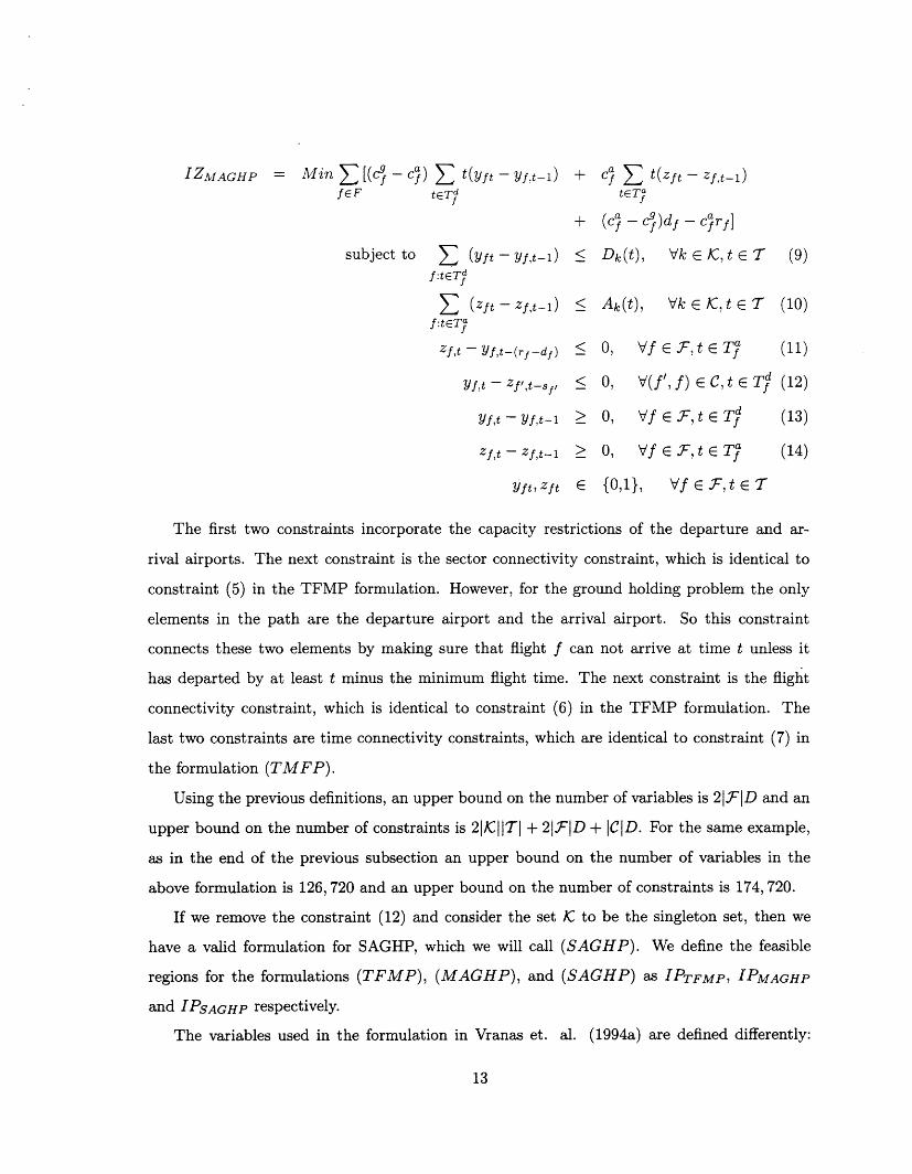
IZMAGHP = Min E [(Cf - c) E t(yft - Yf.t-1) + c' E t(Zft- Zf,t-1)fEF tETd tET7

f f+ (cf - C9)df - Cfrf]

subject to E (ft-yf,t-1) < Dk(t), Vk E K, t E T (9)f:tETf

E (ft-Zf,t-) < Ak(t), VkE CtE (10)f:tE T

Zf,t-Yf,t-(rf-df) < 0, Vf E F, t E T (11)

Yf,t - Zf',t-sf, < O. V(f', f) E C, t E Tf (12)

Yf,t-Yft-1 > 0, Vf E ,t E T/ (13)

zf,t-zf,t-1 > O, Vf E F,t E T (14)

Yft, Zft E {0,1}, Vf Ef,tET

The first two constraints incorporate the capacity restrictions of the departure and ar-

rival airports. The next constraint is the sector connectivity constraint, which is identical to

constraint (5) in the TFMP formulation. However, for the ground holding problem the only

elements in the path are the departure airport and the arrival airport. So this constraint

connects these two elements by making sure that flight f can not arrive at time t unless it

has departed by at least t minus the minimum flight time. The next constraint is the flight

connectivity constraint, which is identical to constraint (6) in the TFMP formulation. The

last two constraints are time connectivity constraints, which are identical to constraint (7) in

the formulation (TMFP).

Using the previous definitions, an upper bound on the number of variables is 21rFID and an

upper bound on the number of constraints is 2jKj1 Tj + 21FlD + ICID. For the same example,

as in the end of the previous subsection an upper bound on the number of variables in the

above formulation is 126,720 and an upper bound on the number of constraints is 174,720.

If we remove the constraint (12) and consider the set KC to be the singleton set, then we

have a valid formulation for SAGHP, which we will call (SAGHP). We define the feasible

regions for the formulations (TFMP), (MAGHP), and (SAGHP) as IPTFMP, IPMAGHP

and IPSAGHP respectively.

The variables used in the formulation in Vranas et. al. (1994a) are defined differently:

13

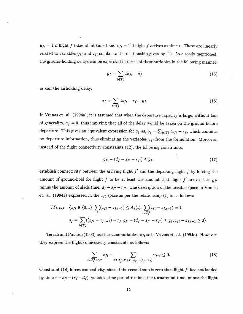
uft = 1 if flight f takes off at time t and vft = 1 if flight f arrives at time t. These are linearly

related to variables Yft and zft similar to the relationship given by (1). As already mentioned,

the ground-holding delays can be expressed in terms of these variables in the following manner:

gf= tuft - df (15)tETd

as can the airholding delay,

af = tft - rf - gf. (16)teTa

In Vranas et. al. (1994a), it is assumed that when the departure capacity is large, without loss

of generality, af = 0, thus implying that all of the delay would be taken on the ground before

departure. This gives an equivalent expression for gf as, gf = EtETf tft - rf, which contains

no departure information, thus eliminating the variables uft from the formulation. Moreover,

instead of the flight connectivity constraints (12), the following constraints,

gf' - (df - Sf - rf,) < gf, (17)

establish connectivity between the arriving flight f' and the departing flight f by forcing the

amount of ground-hold for flight f to be at least the amount that flight f' arrives late gf,

minus the amount of slack time, df - s, - rf,. The description of the feasible space in Vranas

et. al. (1994a) expressed in the zft space as per the relationship (1) is as follows:

IPVBO= {Zft E {O, 1)1 (zft - Zf,t-1) < Ak(t), (zft - Zf,t-1) = 1,f teoT

gf = -t(zft - Zft-1) - rf, g - (df - Sf - rf,) < f, Zft - Zft-l > )teT7

Terrab and Paulose (1993) use the same variables, vft as in Vranas et. al. (1994a). However,

they express the flight connectivity constraints as follows:

E vft- E Vft <O. (18)tETj,t<T t'ETf,t'tr-sf -(rf-df)

Constraint (18) forces connectivity, since if the second sum is zero then flight f' has not landed

by time r - sf, - (rf - df), which is time period r minus the turnaround time, minus the flight

14

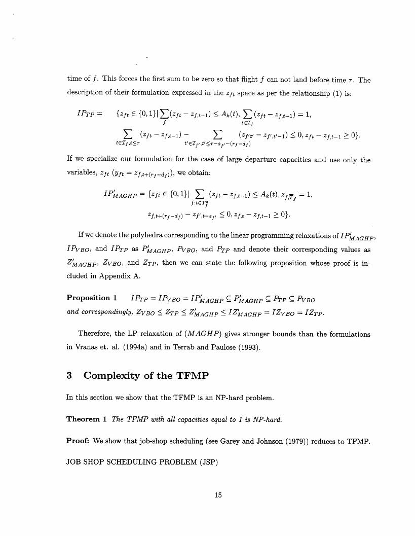
time of f. This forces the first sum to be zero so that flight f can not land before time r. The

description of their formulation expressed in the zft space as per the relationship (1) is:

IPTP = zft E {0, 11 (zft - zf,t-1) < Ak(t), E (zft - Zf,t-1) = 1,f tEzf

E (zft - Zf,t) - E (z? - Zf',t'_1) < O, Zft - Zft-l > .tElzf ,t<r t'Elf ,t' <r-sf/ - (rf-df )

If we specialize our formulation for the case of large departure capacities and use only the

variables, Zft (Yft = Zf,t+(rf-df)), we obtain:

IPMAGHP = {Zft E {O, 1}1 E (zft - Zf,t-) < Ak(t), ZfT = 1,f:tET

Zf,t+(rf-df) - Zf',t-sf < O, Zf,t - Zf,t- 1 > 0}.

If we denote the polyhedra corresponding to the linear programming relaxations of IPMAGHP,

IPVBO, and IPTP as PMAGHP PVBO, and PTP and denote their corresponding values as

ZMAGHP, ZVBO, and ZTP, then we can state the following proposition whose proof is in-

cluded in Appendix A.

Proposition 1 IPTP = IPVBO = IPMAGHP PAGHP C PTP C PVBO

and correspondingly, ZVBO < ZTP < ZMAGHP < IZMAGHP = IZVBO = IZTp.

Therefore, the LP relaxation of (MAGHP) gives stronger bounds than the formulations

in Vranas et. al. (1994a) and in Terrab and Paulose (1993).

3 Complexity of the TFMP

In this section we show that the TFMP is an NP-hard problem.

Theorem 1 The TFMP with all capacities equal to 1 is NP-hard.

Proof: We show that job-shop scheduling (see Garey and Johnson (1979)) reduces to TFMP.

JOB SHOP SCHEDULING PROBLEM (JSP)

15

INSTANCE: Number m E Z + of processors, set J of jobs, each j E J consisting of an ordered

collection of tasks tk[j], I < k < nj, for each task t a length (t) E Z+ and a processor

p(t) E {1, 2,... , m}, where p(tk[j]) - p(tk+l[j]) for all j E J and 1 < k < nj, and a deadline

DE Z + .

QUESTION: Is there a job-shop schedule for J that meets the overall deadline, i.e., a collection

of one-processor schedules ai mapping {t : p(t) = i} into Z-, 1 < i < m, such that ai(t) > ai(t')

implies i (t) > ai (t')+l(t), such that uai'(tk+l[jl) > i (tk[j])+l(tkj]) where i' = p(tk+l[j]) and

i = p(tk[j]), for all j E J and 1 < k < nj, and such that for all j E J, i(tn[j] []) + l(tnj [j]) < D

where i = p(tj [j])?

For each job we create an aircraft. For each processor we associate an airport or sector.

Task tk[j] of job j corresponds to a flight segment, fk[j] of aircraft j. Given a collection of

tasks, tk[] of job j, we associate a list of airports and sectors to be visited by aircraft j.

Furthermore, the processing time of task tk [j] corresponds to the time required to perform the

flight segment, fk [j]. We obtain a list of airports and sectors, (Al, S,.. ., A~, Sk +1,..., AnJ),

and a list of the flight segment times, (t t, t , tk+1 t for each aircraft j by theA," Si ' Si 3' for each aircraft j by the

relationships:

Al = p(tj[1]), t = l(tj[1])

S2 = p(tj[2]), t = (tj [2])

S? = p(tj[3]), t3 = (tj[3])

A . = p(tj[nj]), tA = (tj[nj])

So by finding a job-shop schedule that satifies the given conditions, we will find a solution to

the transformed problem such that all flights are performed by the deadline D. Also, according

to the relationship ai(tk+l[j]) > cai(tkl]) + (tk[j]) where i' = p(tk+l[j]) and i = p(tk[]), no

two tasks will ever performed simultaneously on the same processor, which is equivalent to

limiting the capacities of airports and sectors to one. Moreover, the relationship, ai(t) > i(t')

implies oi(t) > ai(t') + I(t), dictates that a task can not be processed unless the previous

16

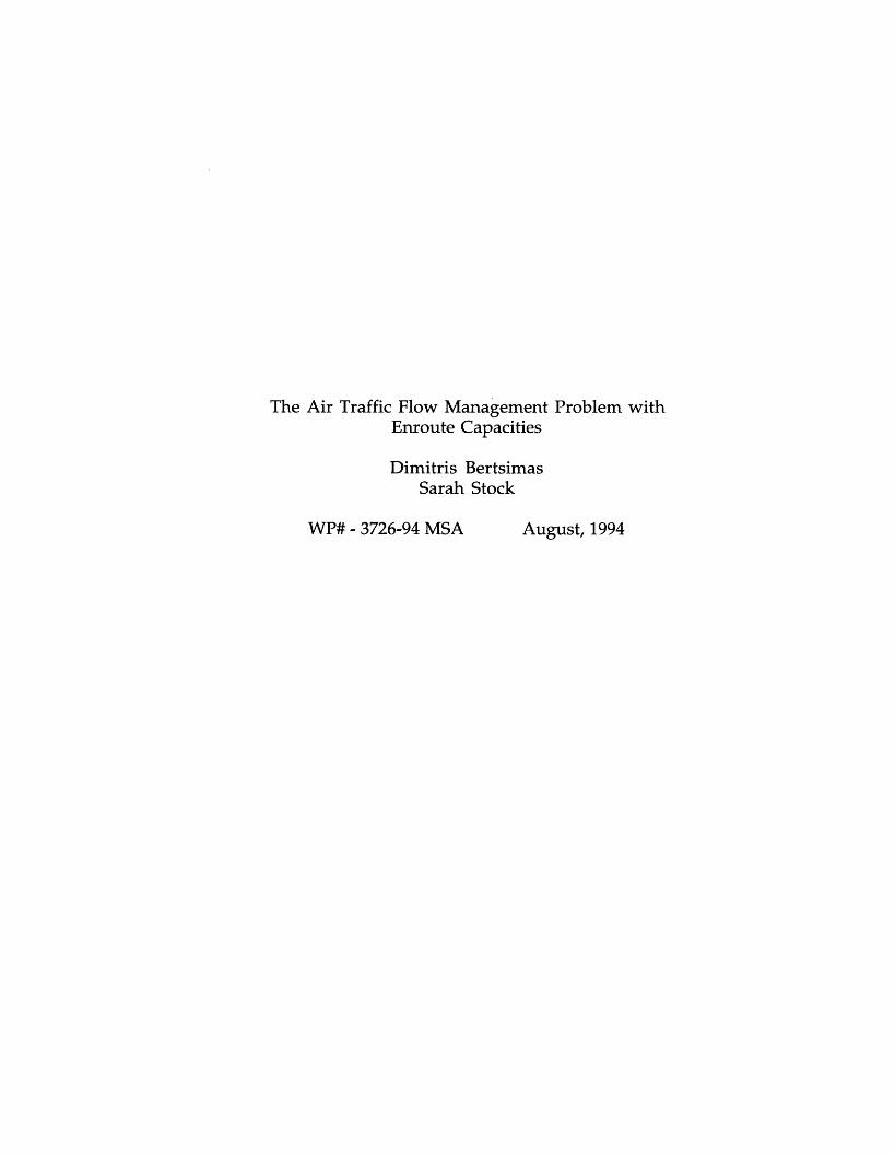
15R 15L

27

4K 33L

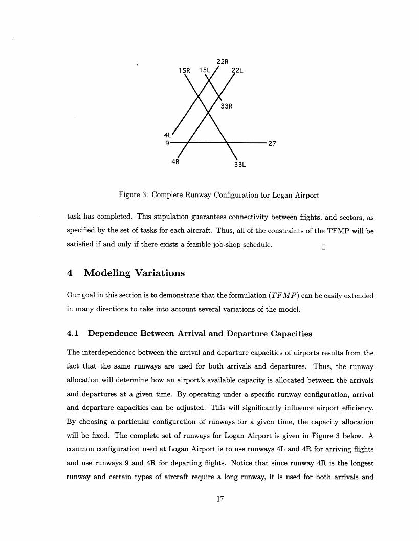
Figure 3: Complete Runway Configuration for Logan Airport

task has completed. This stipulation guarantees connectivity between flights, and sectors, as

specified by the set of tasks for each aircraft. Thus, all of the constraints of the TFMP will be

satisfied if and only if there exists a feasible job-shop schedule. 0

4 Modeling Variations

Our goal in this section is to demonstrate that the formulation (TFMP) can be easily extended

in many directions to take into account several variations of the model.

4.1 Dependence Between Arrival and Departure Capacities

The interdependence between the arrival and departure capacities of airports results from the

fact that the same runways are used for both arrivals and departures. Thus, the runway

allocation will determine how an airport's available capacity is allocated between the arrivals

and departures at a given time. By operating under a specific runway configuration, arrival

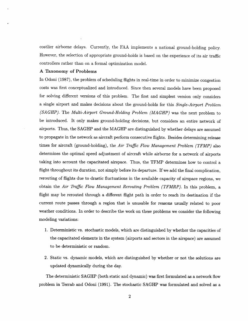
and departure capacities can be adjusted. This will significantly influence airport efficiency.

By choosing a particular configuration of runways for a given time, the capacity allocation

will be fixed. The complete set of runways for Logan Airport is given in Figure 3 below. A

common configuration used at Logan Airport is to use runways 4L and 4R for arriving flights

and use runways 9 and 4R for departing flights. Notice that since runway 4R is the longest

runway and certain types of aircraft require a long runway, it is used for both arrivals and

17

2L

Ak(t)

52

) = 3*62

D(t)62

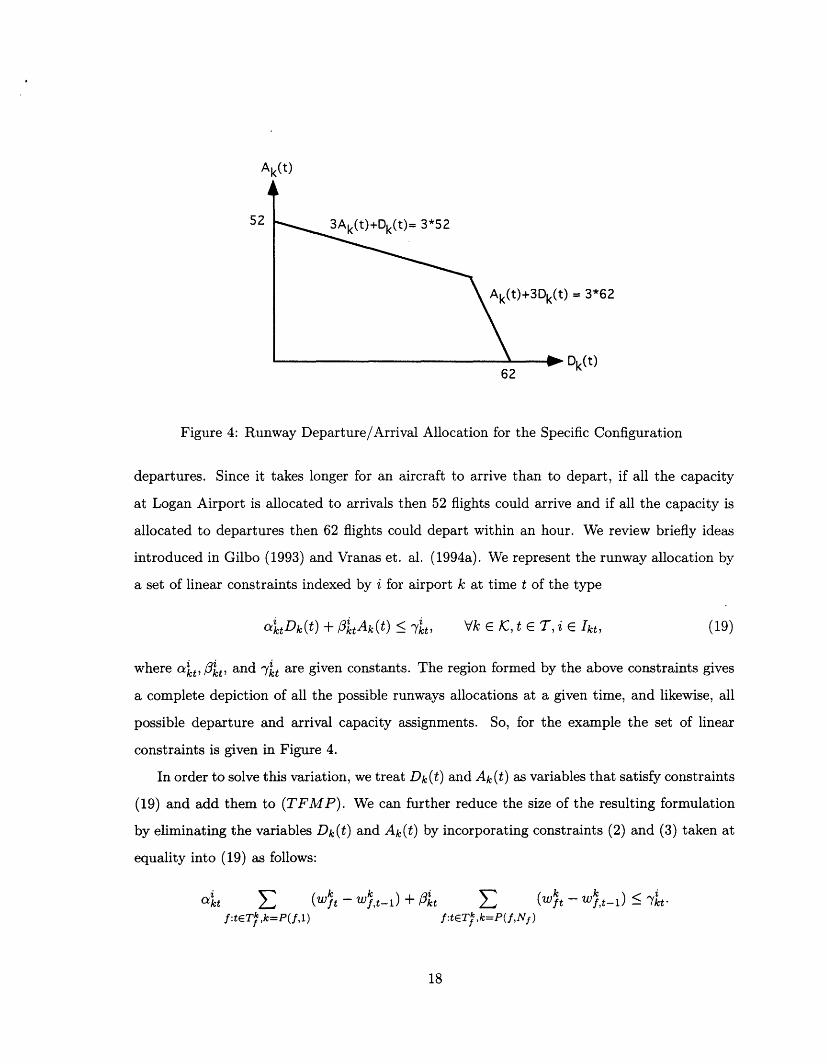
Figure 4: Runway Departure/Arrival Allocation for the Specific Configuration

departures. Since it takes longer for an aircraft to arrive than to depart, if all the capacity

at Logan Airport is allocated to arrivals then 52 flights could arrive and if all the capacity is

allocated to departures then 62 flights could depart within an hour. We review briefly ideas

introduced in Gilbo (1993) and Vranas et. al. (1994a). We represent the runway allocation by

a set of linear constraints indexed by i for airport k at time t of the type

attDk(t) + 3ktAk(t) < Akt Vk E K, t E T, i E Ikt, (19)

where akt, Okt, and %kt are given constants. The region formed by the above constraints gives

a complete depiction of all the possible runways allocations at a given time, and likewise, all

possible departure and arrival capacity assignments. So, for the example the set of linear

constraints is given in Figure 4.

In order to solve this variation, we treat Dk (t) and Ak (t) as variables that satisfy constraints

(19) and add them to (TFMP). We can further reduce the size of the resulting formulation

by eliminating the variables Dk(t) and Ak(t) by incorporating constraints (2) and (3) taken at

equality into (19) as follows:

f t (WT~,Wt1) + 3k (Wt tk1) < Aif:tETfk=P(fl) f:tETfk ,k=P(f,Nf)

18

The addition of this constraint to (TFMP) incorporates the dependence between the arrival

and departure capacity assignments without the addition of any new variables.

4.2 Hub Connectivity with Multiple Connections

Given that many airlines now control key hub airports through which most of their flights are

directed, it is no longer obvious which aircraft will fly a subsequent flight. At these hubs, many

airplanes are capable of performing any one of multiple consecutive flights. We refer to the

issue of assigning aircraft to continuing flights as hub connectivity. This can be achieved by

extending the model as follows:

For each arriving flight f' that is continued there is a set of flights Rf, that can continue flight

f'. Introducing the 0 - 1 variables XfIf, which take on the value 1 if flight f' is continued by

flight f E Rf, and 0 otherwise, we alter constraint (6) as follows

Wt - Wk, t-S 1- Xf'f, V(f', f) E C, t E Tk k = P(f, 1) = P(f', Nf)ft f,t-$fI - 1 f- ( f ,

and add the constraint that each continued flight f' has to be assigned to a flight in Rf,:

E Xff l.fERf,

4.3 Banks of Flights

With the evolution of the hub and spoke system, airlines have a set of flights (banks) that are

scheduled to arrive at a hub airport and another set scheduled to depart within a small time

window of the arrival bank. Each arriving aircraft will be assigned to perform at most one of

the departing flights. This situation is similar to hub connectivity, except that airlines seek to

minimize the time between the departure of the first and the last flight in the bank. Let B be

the set of flights in a bank. We define the decision variables

1 if the first flight f in B arrives by time tYB,t =

0 otherwise

1 if the last flight f in B arrives by time tZB,t = otherwise

0 otherwise

19

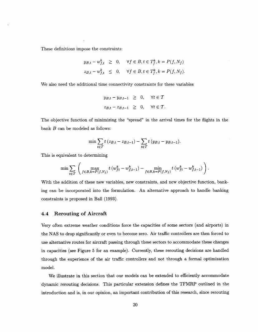
These definitions impose the constraints:

YB,t-Wf,t -O, Vf E B, t E T , k = P(f, N)

ZB,t -Wt < 0, Vf E B, t E Tf, k P(f, N).

We also need the additional time connectivity constraints for these variables

YB,t-YB,t-1 > O, Vt E T

ZB,t -ZB,t-1 > O, Vt E E.

The objective function of minimizing the "spread" in the arrival times for the flights in the

bank B can be modeled as follows:

min t (ZB,t - ZB,t-1) - t (YB,t - YB,t-1).teT tET

This is equivalent to determining

mmn E ( max t (Wkt-f -l min t (Wkt - wk) kw

tET fEB,k=P(f,Nf) fEB,k=P(f,Nf) ft

With the addition of these new variables, new constraints, and new objective function, bank-

ing can be incorporated into the formulation. An alternative approach to handle banking

constraints is proposed in Ball (1993).

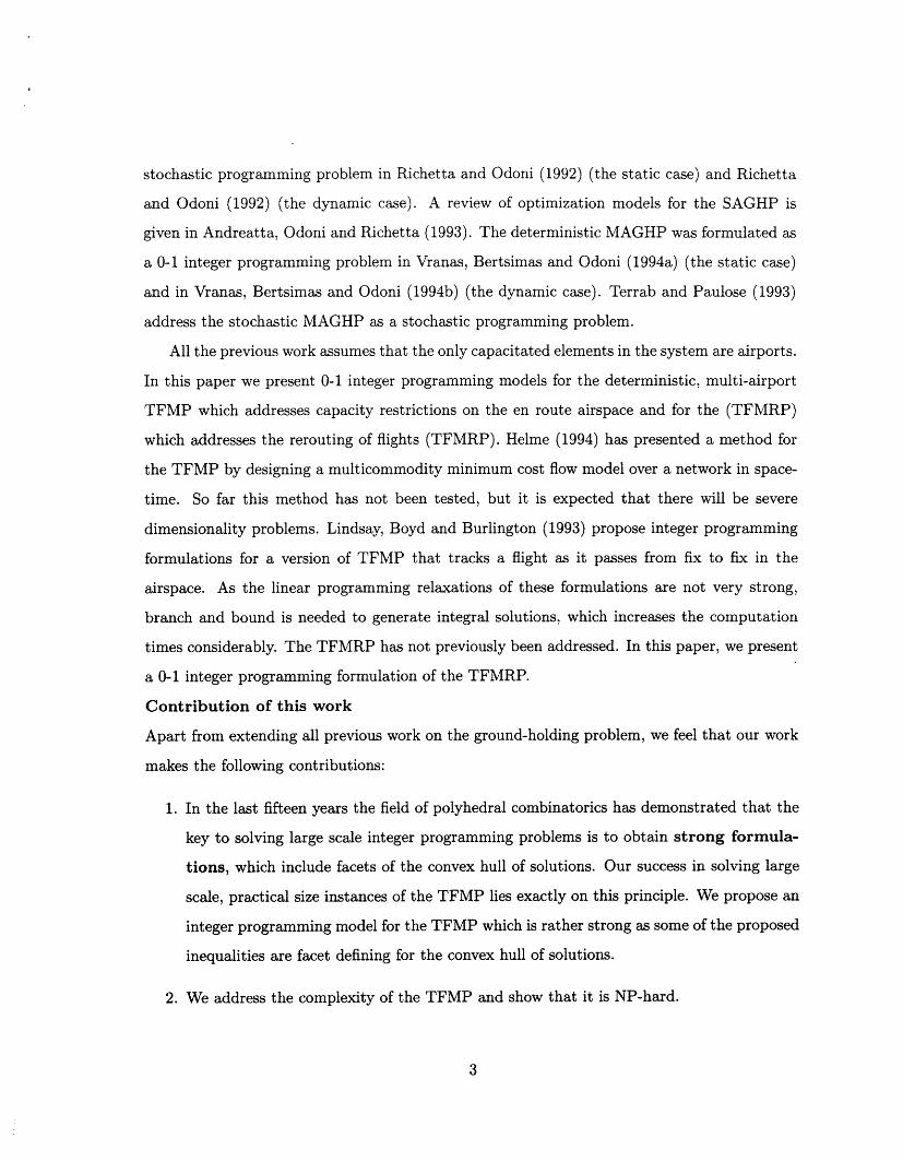
4.4 Rerouting of Aircraft

Very often extreme weather conditions force the capacities of some sectors (and airports) in

the NAS to drop significantly or even to become zero. Air traffic controllers are then forced to

use alternative routes for aircraft passing through these sectors to accommodate these changes

in capacities (see Figure 5 for an example). Currently, these rerouting decisions are handled

through the experience of the air traffic controllers and not through a formal optimization

model.

We illustrate in this section that our models can be extended to efficiently accommodate

dynamic rerouting decisions. This particular extension defines the TFMRP outlined in the

introduction and is, in our opinion, an important contribution of this research, since rerouting

20

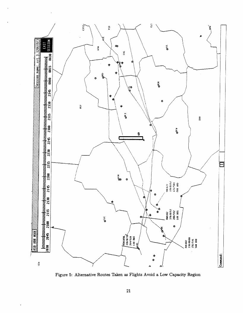
Figure 5: Alternative Routes Taken as Flights Avoid a Low Capacity Region

21

of aircraft is a very common practice in air traffic control, that has not yet been addressed in

the literature.

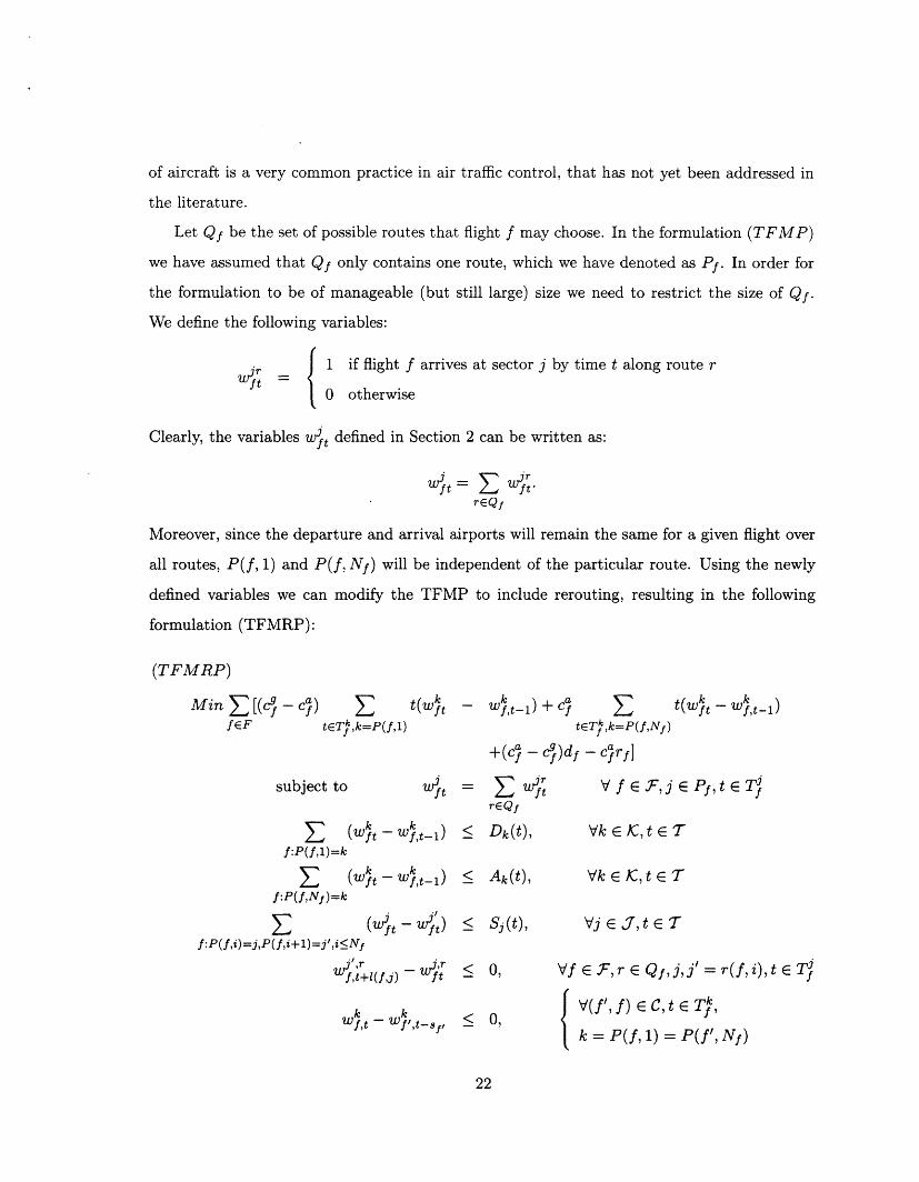
Let Qf be the set of possible routes that flight f may choose. In the formulation (TFMP)

we have assumed that Qf only contains one route, which we have denoted as Pf. In order for

the formulation to be of manageable (but still large) size we need to restrict the size of Qf.

We define the following variables:

wArft

1 if flight f arrives at sector j by time t along route r

0 otherwise

Clearly, the variables w3ft defined in Section 2 can be written as:

reQf

Moreover, since the departure and arrival airports will remain the same for a given flight over

all routes, P(f, 1) and P(f, Nf) will be independent of the particular route. Using the newly

defined variables we can modify the TFMP to include rerouting, resulting in the following

formulation (TFMRP):

(TFMRP)

Min [(Cf -ca) )fEF teTk,k=P(f,1)

subject to

t(wk,

Witft

E (wkt -Wt-1)f:P(f,1)=k

E (Wt - W,t-1)f:P(f,Nf)=k

E (wt - wi)f:P(f,i)=j,P(f ,i+l )=j',i <Nf

f,t+1(fj) ft

Wft- Wf ,t-sflf ,t k

- Wft-1) + Ca 5 t(w -f t)

tETfk,k=P(f,Nf)

+(cf- c9f)df- Cf rf]

= Zd jr VfEF,jEPf,tETfrEQf

< Dk(t), Vk E IC,t E T

< Ak(t), Vk E KC,t E T

Sj (t), V E , t E T

< 0, Vf E F,r E Qf,j,j' = r(f,i),t E Tf

< 0, V(f',f)E C,tETfk Ek = P(f, 1) = P(f', Nf)

22

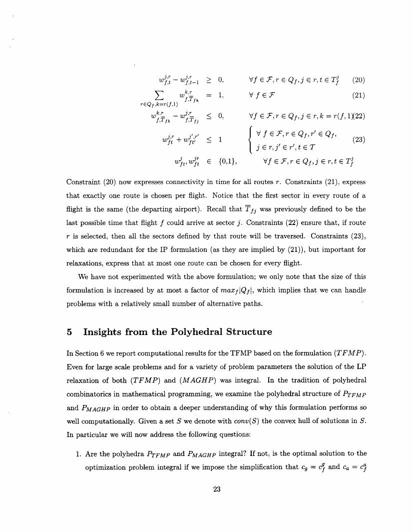
3j.r - j r wft- w ft- 1 > , Vf E ,r E Qf,j Er, t E T (20)

rEf f1 W;k = 1, VfE F (21)wf,TfkrEQf,k=r(f,l)

r < ,T `0, Vf E fE, r E Qf,j E r, k = r(f, 1X22)f,Tfk f,Tfj

rV f E F, r E Qfr' E Qf, (23)wjft + j t/ < 1 i r,j' E r',t E T (23)

jfat, wit E {0,1}, Vf E F,r E Qf,j E r,t E T½

Constraint (20) now expresses connectivity in time for all routes r. Constraints (21), express

that exactly one route is chosen per flight. Notice that the first sector in every route of a

flight is the same (the departing airport). Recall that Tfj was previously defined to be the

last possible time that flight f could arrive at sector j. Constraints (22) ensure that, if route

r is selected, then all the sectors defined by that route will be traversed. Constraints (23),

which are redundant for the IP formulation (as they are implied by (21)), but important for

relaxations, express that at most one route can be chosen for every flight.

We have not experimented with the above formulation; we only note that the size of this

formulation is increased by at most a factor of maxflQfl, which implies that we can handle

problems with a relatively small number of alternative paths.

5 Insights from the Polyhedral Structure

In Section 6 we report computational results for the TFMP based on the formulation (TFMP).

Even for large scale problems and for a variety of problem parameters the solution of the LP

relaxation of both (TFMP) and (MAGHP) was integral. In the tradition of polyhedral

combinatorics in mathematical programming, we examine the polyhedral structure of PTFMP

and PMAGHP in order to obtain a deeper understanding of why this formulation performs so

well computationally. Given a set S we denote with conv(S) the convex hull of solutions in S.

In particular we will now address the following questions:

1. Are the polyhedra PTFMP and PMAGHP integral? If not, is the optimal solution to the

optimization problem integral if we impose the simplification that cg = c9f and Ca = cf

23

for all f E F?

2. Are the constraints in (TFMP) and (MAGHP) facets of conv(IPTFMP) and COnV(IPMAGHP)

respectively?

We summarize our findings in the following theorem:

Theorem 2

1. The polyhedra PTFMP and PMAGHP are not integral even with the simplification that

cg = c9f and Ca = cf for all f E F.

2. Inequalities (10), (11) and (12) are facets for conv(IPMAGHP), while the constraints (8)

and (9) are not. Inequalities (4), (5) and (6) are facets for conv(IPTFMP), while the

constraints (1), (2) and (3) are not.

As the proofs of the theorem are somewhat technical, we have placed them in appendices B,

and C respectively.

The previous theorem gives some partial insight on the usefulness of the new variables

we introduced, which make it easy to express sharply the various types of connectivity in

the problem. While the formulations are not integral, the inequalities that the three types

of connectivity impose are indeed facets. As the solutions obtained were integral for a wide

spectrum of examples and parameters, we did not investigate further the determination of

other facets.

6 Insights from computations

In this section we report the results of a series of computational experiments that we conducted.

In performing the computational experiments we aim to address the following questions:

1. How frequently are the solutions obtained by solving the LP relaxations of (TFMP) and

(MAGHP) integral?

2. How is the integrality of solutions affected by the various problem parameters and the

size of the problem?

24

3. How is the computational time required to obtain an optimal solution affected by the

various problem parameters and the size of the problem?

4. How does the present approach compare with other approaches in the literature?

5. Given that the TFMP needs to be solved on line for controlling air traffic in the US,

perhaps the most important question to ask is: How large problems can we solve

in reasonable computational times? In other words, is the present approach a realistic

method to control air traffic in the US?

Ground-Holding Problem Test Cases

We performed computational experiments on datasets used in Vranas et. al. (1994a) on

the Ground-Holding Problem. Specifically, we looked at the datasets consisting of 2 and 6

airports with 500 flights per airport, 1000 and 3000 flights respectively. Some adjustments in

the data were necessary in order to accomodate the differences between the two models. In

particular, the previous model did not include of any departure data, as all of the optimization

was done with respect to arrivals. Thus, we generated departure data (times and capacities)

that were compatible with the existing arrival data.

As in Vranas et. al. (1994a), for each of these cases, four levels of flight connectivity were

considered. These levels give the ratios of continued flight to total flights, ICl/IFl, as 0.20,

0.40, 0.60, and 0.80.

We considered 15 minute time intervals taken over a 16 hour day. All experiments were

performed on a Sun SPARCstation 10 model 41. GAMS was used as the modeling tool and

CPLEXMIP 2.1 was used as the solver. The results that we obtained using the above datasets

and our (MAGHP) formulation are summarized in Tables 1 and 2. Tables 1 and 2 give results

at the infeasibility border for each case. The infeasibility border is the set of critical values for

the departure and arrival capacities under which the problem becomes infeasible. We expect

that it is in this region that the problem is very relevant practically and is harder to solve.

The critical capacity levels were found by a series of trial and error tests. The times reported

are in CPU seconds and the % Nonint column is the percentage of total flights whose solution

was noninteger. If we compare these results with the results from Vranas et. al. (1994a) (see

25

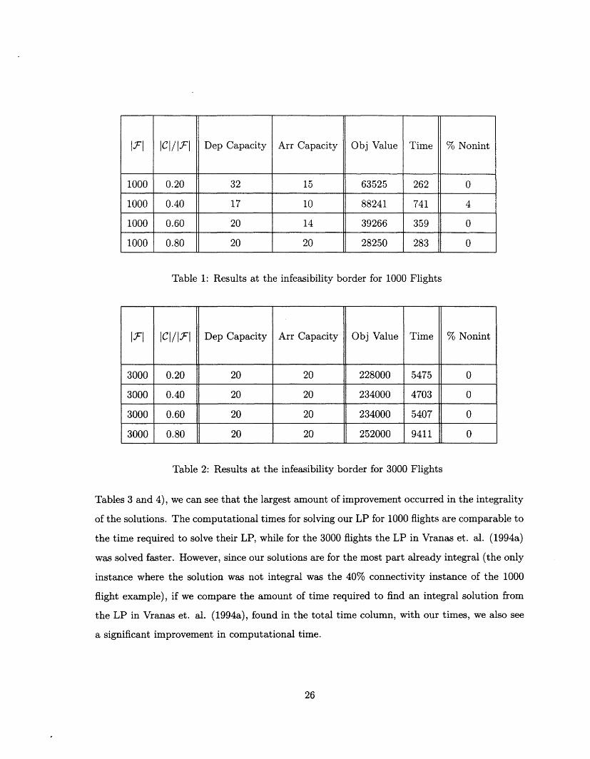
IFI ICI/IFI Dep Capacity Arr Capacity Obj Value Time % Nonint

1000 0.20 32 15 63525 262 0

1000 0.40 17 10 88241 741 4

1000 0.60 20 14 39266 359 0

1000 0.80 20 20 28250 283 0

Table 1: Results at the infeasibility border for 1000 Flights

F ICl/I.F Dep Capacity Arr Capacity Obj Value Time % Nonint

3000 0.20 20 20 228000 5475 0

3000 0.40 20 20 234000 4703 0

3000 0.60 20 20 234000 5407 0

3000 0.80 20 20 252000 9411 0

Table 2: Results at the infeasibility border for 3000 Flights

Tables 3 and 4), we can see that the largest amount of improvement occurred in the integrality

of the solutions. The computational times for solving our LP for 1000 flights are comparable to

the time required to solve their LP, while for the 3000 flights the LP in Vranas et. al. (1994a)

was solved faster. However, since our solutions are for the most part already integral (the only

instance where the solution was not integral was the 40% connectivity instance of the 1000

flight example), if we compare the amount of time required to find an integral solution from

the LP in Vranas et. al. (1994a), found in the total time column, with our times, we also see

a significant improvement in computational time.

26

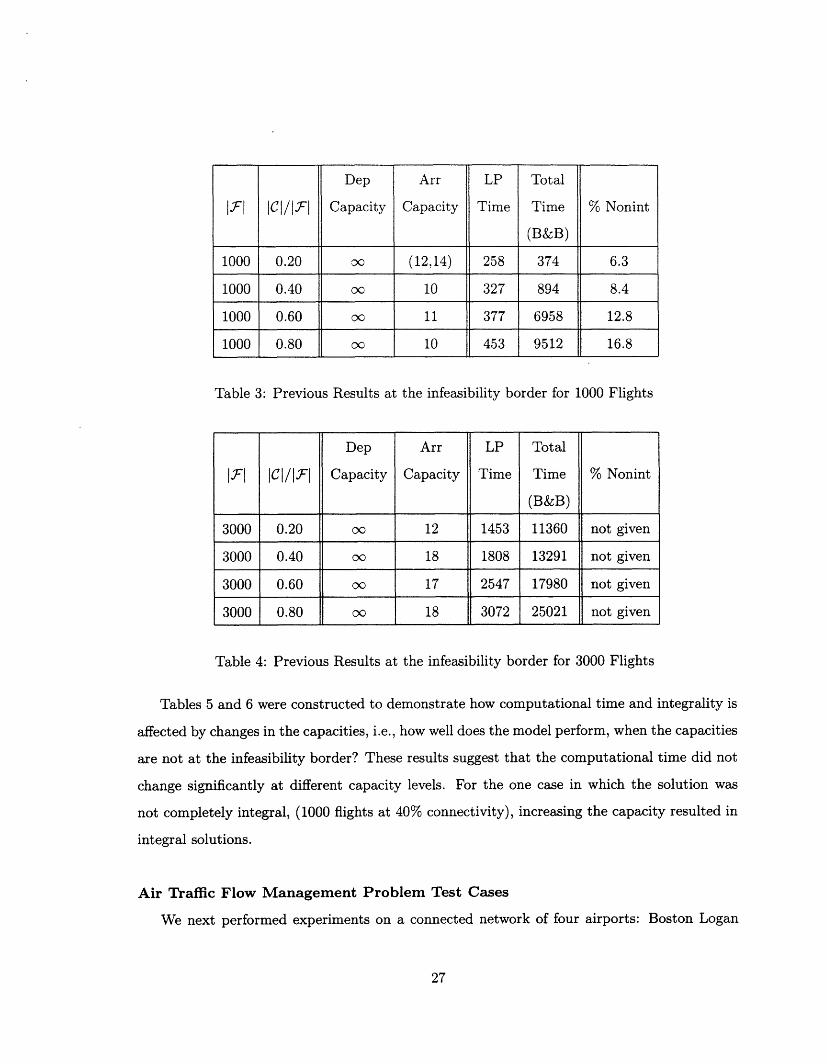
Dep Arr LP Total

I.F CI/Ft Capacity Capacity Time Time % Nonint

(B&B)

1000 0.20 cx (12,14) 258 374 6.3

1000 0.40 co 10 327 894 8.4

1000 0.60 00 11 377 6958 12.8

1000 0.80 00 10 453 9512 16.8

Table 3: Previous Results at the infeasibility border for 1000 Flights

Dep Arr LP Total

F1 IC 1/J 1 Capacity Capacity Time Time % Nonint

,___I__ _ I.(B&B)

3000 0.20 o 12 1453 11360 not given

3000 0.40 oo 18 1808 13291 not given

3000 0.60 oo 17 2547 17980 not given

3000 0.80 oo 18 3072 25021 not given

Table 4: Previous Results at the infeasibility border for 3000 Flights

Tables 5 and 6 were constructed to demonstrate how computational time and integrality is

affected by changes in the capacities, i.e., how well does the model perform, when the capacities

are not at the infeasibility border? These results suggest that the computational time did not

change significantly at different capacity levels. For the one case in which the solution was

not completely integral, (1000 flights at 40% connectivity), increasing the capacity resulted in

integral solutions.

Air Traffic Flow Management Problem Test Cases

We next performed experiments on a connected network of four airports: Boston Logan

27

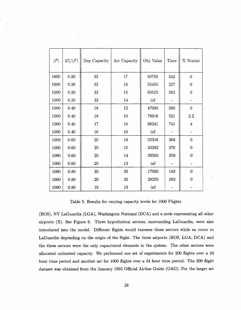
Table 5: Results for varying capacity levels for 1000 Flights

(BOS), NY LaGuardia (LGA), Washington National (DCA) and a node representing all other

airports (X). See Figure 6. Three hypothetical sectors, surrounding LaGuardia, were also

introduced into the model. Different flights would traverse these sectors while en route to

LaGuardia depending on the origin of the flight. The three airports (BOS, LGA, DCA) and

the three sectors were the only capacitated elements in the system. The other sectors were

allocated unlimited capacity. We performed one set of experiments for 200 flights over a 24

hour time period and another set for 1000 flights over a 24 hour time period. The 200 flight

dataset was obtained from the January 1993 Official Airline Guide (OAG). For the larger set

28

I1 ICI/I.1 Dep Capacity Arr Capacity Obj Value Time % Nonint

1000 0.20 32 17 50750 342 0

1000 0.20 32 16 55450 227 0

1000 0.20 32 15 63525 262 0

1000 0.20 32 14 inf - -

1000 0.40 18 12 47000 290 0

1000 0.40 18 10 79916 521 2.2

1000 0.40 17 10 88241 741 4

1000 0.40 16 10 inf - -

1000 0.60 20 18 22316 369 0

1000 0.60 20 15 33292 376 0

1000 0.60 20 14 39266 359 0

1000 0.60 20 13 inf - -

1000 0.80 30 30 17000 183 0

1000 0.80 20 20 28250 283 0

1000 0.80 19 19 inf -

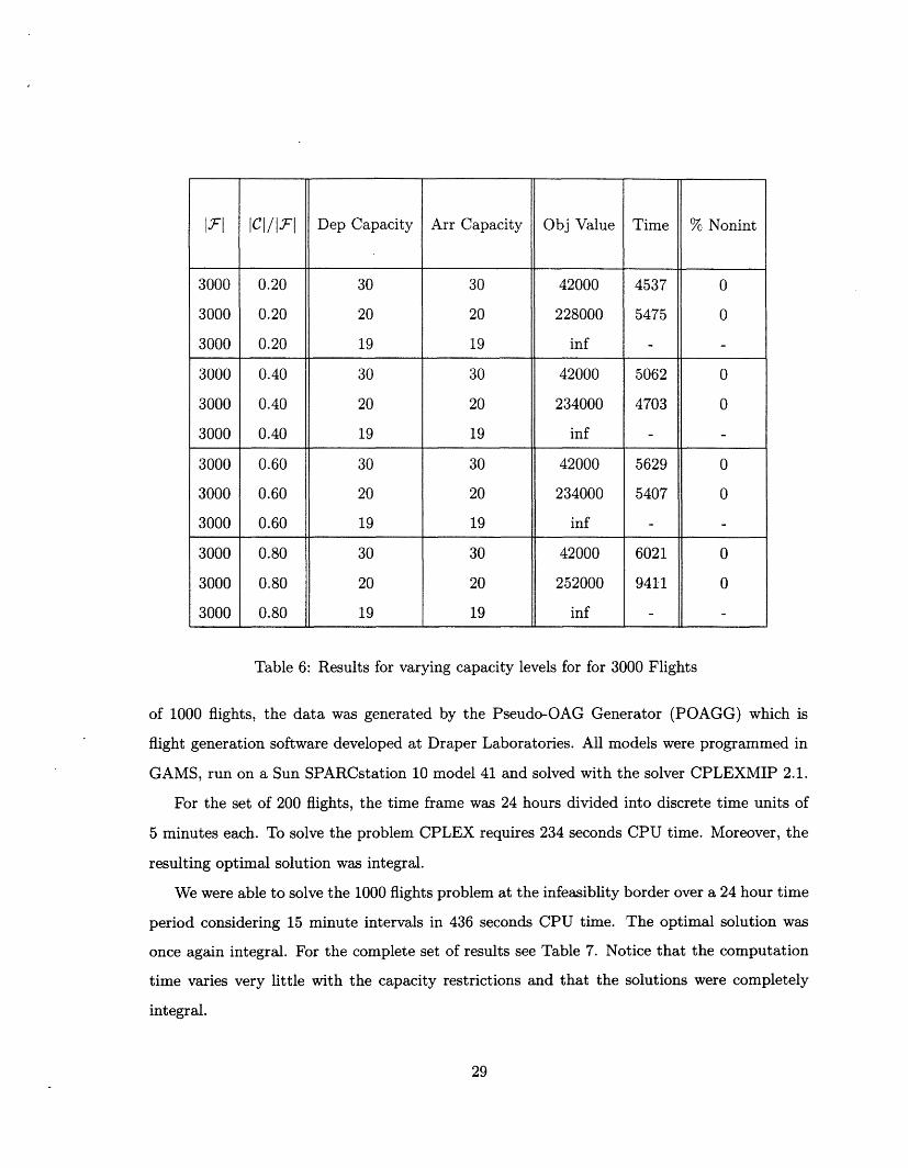
Table 6: Results for varying capacity levels for for 3000 Flights

of 1000 flights, the data was generated by the Pseudo-OAG Generator (POAGG) which is

flight generation software developed at Draper Laboratories. All models were programmed in

GAMS, run on a Sun SPARCstation 10 model 41 and solved with the solver CPLEXMIP 2.1.

For the set of 200 flights, the time frame was 24 hours divided into discrete time units of

5 minutes each. To solve the problem CPLEX requires 234 seconds CPU time. Moreover, the

resulting optimal solution was integral.

We were able to solve the 1000 flights problem at the infeasiblity border over a 24 hour time

period considering 15 minute intervals in 436 seconds CPU time. The optimal solution was

once again integral. For the complete set of results see Table 7. Notice that the computation

time varies very little with the capacity restrictions and that the solutions were completely

integral.

29

Fl I CI/FI Dep Capacity Arr Capacity Obj Value Time % Nonint

3000 0.20 30 30 42000 4537 0

3000 0.20 20 20 228000 5475 0

3000 0.20 19 19 inf -

3000 0.40 30 30 42000 5062 0

3000 0.40 20 20 234000 4703 0

3000 0.40 19 19 inf -

3000 0.60 30 30 42000 5629 0

3000 0.60 20 20 234000 5407 0

3000 0.60 19 19 inf - -

3000 0.80 30 30 42000 6021 0

3000 0.80 20 20 252000 941-1 0

3000 0.80 19 19 inf -

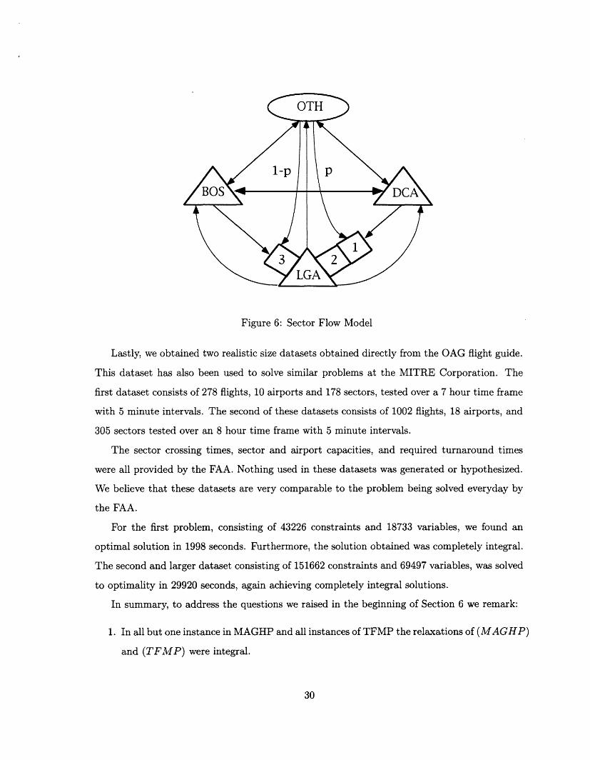
Figure 6: Sector Flow Model

Lastly, we obtained two realistic size datasets obtained directly from the OAG flight guide.

This dataset has also been used to solve similar problems at the MITRE Corporation. The

first dataset consists of 278 flights, 10 airports and 178 sectors, tested over a 7 hour time frame

with 5 minute intervals. The second of these datasets consists of 1002 flights, 18 airports, and

305 sectors tested over an 8 hour time frame with 5 minute intervals.

The sector crossing times, sector and airport capacities, and required turnaround times

were all provided by the FAA. Nothing used in these datasets was generated or hypothesized.

We believe that these datasets are very comparable to the problem being solved everyday by

the FAA.

For the first problem, consisting of 43226 constraints and 18733 variables, we found an

optimal solution in 1998 seconds. Furthermore, the solution obtained was completely integral.

The second and larger dataset consisting of 151662 constraints and 69497 variables, was solved

to optimality in 29920 seconds, again achieving completely integral solutions.

In summary, to address the questions we raised in the beginning of Section 6 we remark:

1. In all but one instance in MAGHP and all instances of TFMP the relaxations of (MAGHP)

and (TFMP) were integral.

30

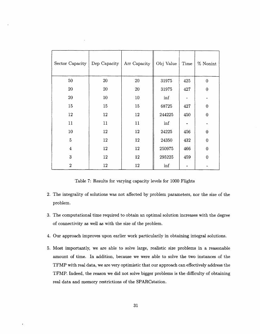
Table 7: Results for varying capacity levels for 1000 Flights

2. The integrality of solutions

problem.

was not affected by problem parameters, nor the size of the

3. The computational time required to obtain an optimal solution increases with the degree

of connectivity as well as with the size of the problem.

4. Our approach improves upon earlier work particularily in obtaining integral solutions.

5. Most importantly, we are able to solve large, realistic size problems in a reasonable

amount of time. In addition, because we were able to solve the two instances of the

TFMP with real data, we are very optimistic that our approach can effectively address the

TFMP. Indeed, the reason we did not solve bigger problems is the difficulty of obtaining

real data and memory restrictions of the SPARCstation.

31

Sector Capacity Dep Capacity Arr Capacity Obj Value Time % Nonint

50 20 20 31975 425 0

20 20 20 31975 427 0

20 10 10 inf - -

15 15 15 68725 427 0

12 12 12 244225 450 0

11 11 11 inf - -

10 12 12 24225 456 0

5 12 12 24350 432 0

4 12 12 250975 466 0

3 12 12 295225 459 0

2 12 12 inf - -

7 Conclusions

We have presented what we believe is a realistic and practical approach to solve the Air

Traffic Flow Management Problem. Our model takes into account all the capacitated elements

in the system (arrival, departure and sector capacity) and easily extends to incorporate the

dependence of airport runway capacity of departures and arrivals, hub connectivity, banking

and rerouting flights when capacity levels drop drastically. The FAA has been operating for

several years in Washington, D.C. an Air Traffic Control System Command Center (ATCSC),

equipped with outstanding information-gathering capabilities that dynamically keeps track of

all the information about capacities, flight information, weather, etc. We believe that the

present optimization based approach is very well suited to be the optimization "brain" for

this system. We envision that the ATCSC will constantly be optimizing the system using

the formulations developed in this paper. As new information is coming into the system,

the solutions will constantly be updated. Implementing such a system is perhaps the most

challenging task we face.

Acknowledgments

We would like to thank Professor Amedeo Odoni for inspiring our work in this area and being

a constant source of guidance and encouragement during the course of this research. We would

like to thank David Weiner and Thomas Mifflin of the FAA for encouraging and supporting

our work. We would like to thank Dr. Kenneth Lindsay for providing data for some of the

computational experiments, Ms. Wandy Sae-tan for performing some of the computational

experiments and Dr. Eugene Gilbo for providing some of the figures.

32

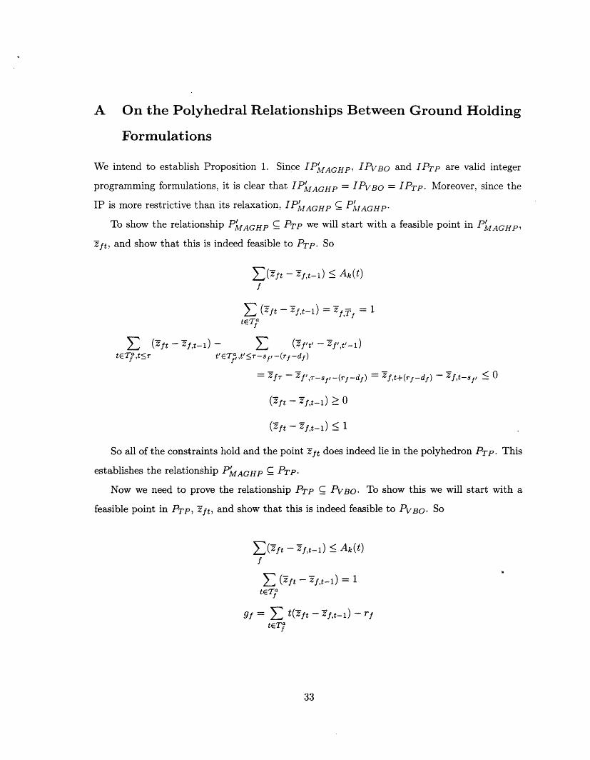
A On the Polyhedral Relationships Between Ground Holding

Formulations

We intend to establish Proposition 1. Since IPNvAGHP, IPVBO and IPTp are valid integer

programming formulations, it is clear that IPAIAGHP = IPVBO = IPTp. Moreover, since the

IP is more restrictive than its relaxation, IPIAGHP C PNIAGHP

To show the relationship PMAGHP C PTP we will start with a feasible point in PMAGHP,

Zft, and show that this is indeed feasible to PTP. So

Z(ft - Zf,t-1) < Ak(t)

f

E (ft - Zft-1) = ZfT = 1te7

Z (Tft - Zf,t-1) - E (fit/ - Zf',t'-1)tETfa,t<T t'ETfa ,t'<7-sf,-(rf -df)

= ZfT- Zf',,r-sf-(rf -df) = Zf,t+(rf-df) - Zf,t-sf, < 0

(5ft - f,t-1) > o

(ft - f,t-1) < 1

So all of the constraints hold and the point Tft does indeed lie in the polyhedron PTP. This

establishes the relationship PMAGHP C PTP.

Now we need to prove the relationship PTP C PVBO. To show this we will start with a

feasible point in PTP, Zft, and show that this is indeed feasible to PVBO So

(Zlft - f,t-) < Ak(t)f

E (ft - f,t-1) = 1tE~

tETt ETfa

33

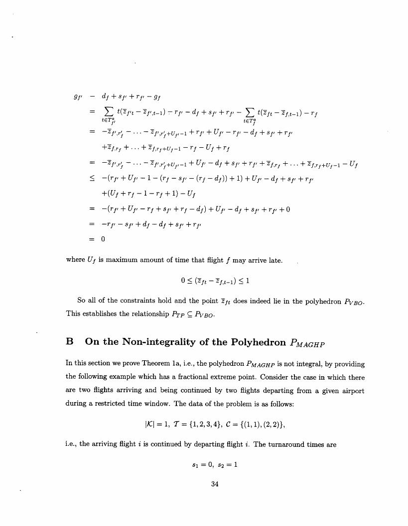
g9' - df +f, +rf'-gf

- Z t(f't - Zf',t-1) rf - df + Sf + rf, - t(ft -Zft-1) - rftET, tETf

- Zf'lr; -* - Zf',r'+Uf,- + rfl + Uf' - rfl - df + Sf1 + rf,

+Zf,rf + ... + Zf,rf+Uf-1 -rf - Uf + rf

-= fIr -f' r} -- f',rj,+Uf,-1 + Uf, - df + Sf, + rf, + Zf,rf + + Zf,rf+Ufl - Uf

< -(r,' + Uf - 1 - (rf - Sf - (f - df)) + 1) + Us, - ds + sf' + f'

+(Uf + rf - 1 - rf + 1) - Uf

= -(rf' + Uf' - rf + sfs + rf - df) + Uf - df + sfl + rf + 0O

= -rf, - Sf + df - df +SfI + rf,

= O

where Uf is maximum amount of time that flight f may arrive late.

0 < (ft- ft-1) < 1

So all of the constraints hold and the point ft does indeed lie in the polyhedron PVBO-

This establishes the relationship PTP C PVBO-

B On the Non-integrality of the Polyhedron PMAGHP

In this section we prove Theorem la, i.e., the polyhedron PMAGHP is not integral, by providing

the following example which has a fractional extreme point. Consider the case in which there

are two flights arriving and being continued by two flights departing from a given airport

during a restricted time window. The data of the problem is as follows:

IKl = 1, T = 1, 2,3,4}, C = (1, 1), (2,2)},

i.e., the arriving flight i is continued by departing flight i. The turnaround times are

81 = 0, S2 = 1

34

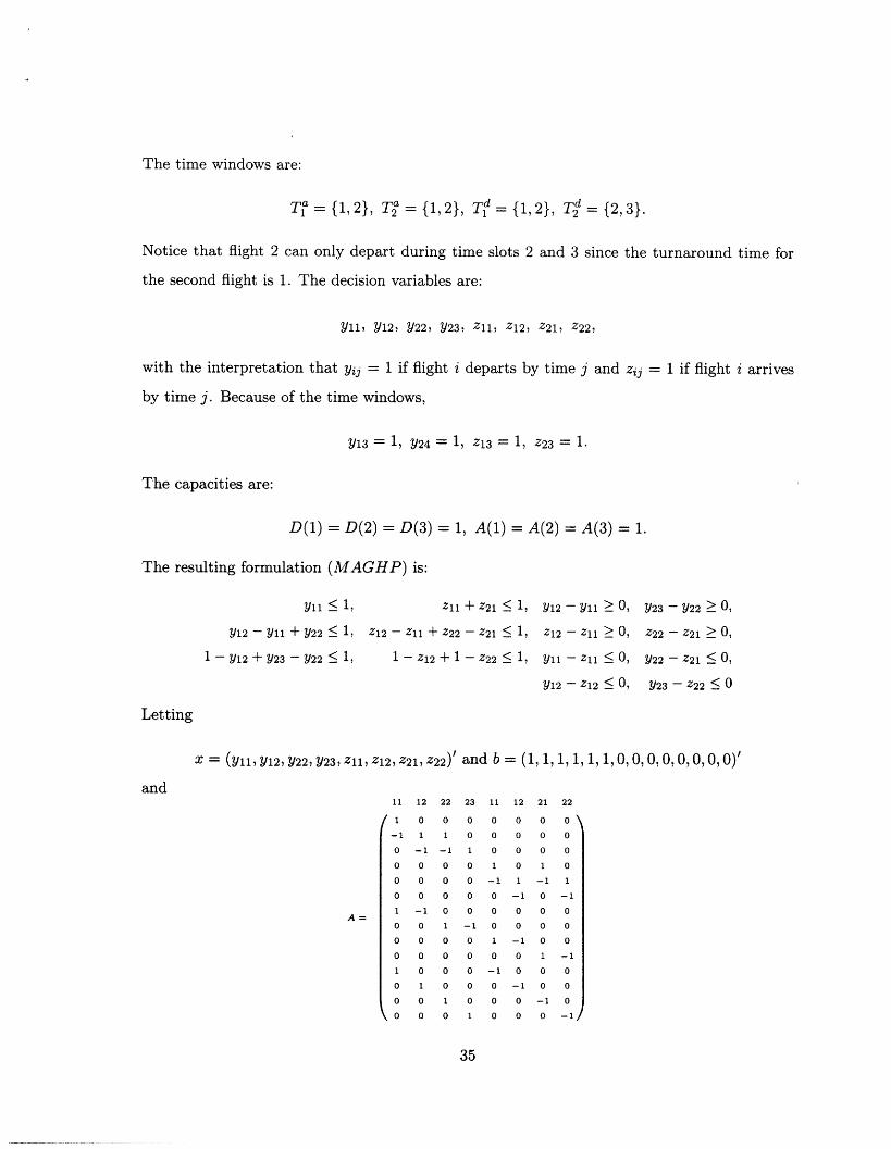
The time windows are:

T = {1,2}, 1,2, T , = {1,2}, T2d = {2,3).

Notice that flight 2 can only depart during time slots 2 and 3 since the turnaround time for

the second flight is 1. The decision variables are:

Y11, Y12, Y22, Y23, Z11, Z12, Z21, Z2 2 ,

with the interpretation that yij = 1 if flight i departs by time j and zij = 1 if flight i arrives

by time j. Because of the time windows,

Y13 = 1, Y24 = 1, Z13 = 1, Z23 =-- 1.

The capacities are:

D(1) = D(2) = D(3) = 1, A(1) = A(2) = A(3) = 1.

The resulting formulation (MAGHP) is:

Yl < , 11 + Z21 < 1, Y12- Y11 > , Y23 - Y22 > 0,

Y12 - Y11 + Y22 1, 12 -- Z11 + Z22 - 21 1, Z12 -Z11 > 0, Z22 - Z21 > 0,

1-Y12 + Y23 - Y22 <, 12 + 1 - 22 <1, Y11l-Z < 0, Y22 - Z21 < 0,

Y12 -Z12 < 0, Y23 - 22 < 0

Letting

x = (Y11, Y12, Y22, Y23, Zll Z12, Z21, Z22) and b = (1,, 1, , 1, 1, 0, 0, 0, 0, 0, 0, 0, 0)'

and11 12 22 23 11 12 21 22

/t n n n n n n \

-1 1 1 0 0 0 0 0

0 -1 1 0 0 0 0

o o 0 0 1 0 1 0

0 0 0 0 -1 1 -1 1

0 0 0 0 0 -1 0 -1

1 -1 0 0 0 0 0 0

0 0 1 -1 0 0 0 0

0 0 0 0 1 -1 0 0

0 0 0 0 0 0 1 -1

1 0 0 0 -1 0 0 0

0 1 0 0 0 -1 0 0

0 0 1 0 0 0 -1 0- - . - .

\U U I U U U -1/

35

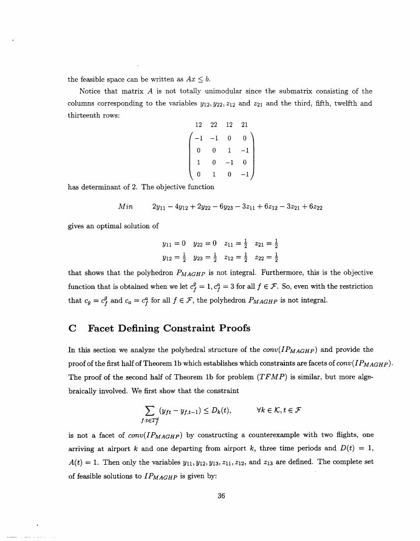
the feasible space can be written as Ax < b.

Notice that matrix A is not totally unimodular since

columns corresponding to the variables Y12, Y22, Z12 and z21

thirteenth rows:

has determinant of 2. The objective

Min

12 22

-1 -1

0 0

1 0

0 1

function

12

0

1

-1

0

the submatrix consisting of the

and the third, fifth, twelfth and

21

0

-1

0

-1

2 y11 - 4 Y12 + 2 y22 - 6 Y23 - 3z1 1 + 6z12 - 3Z2 1 + 6z2 2

gives an optimal solution of

Y11 =-- 0

1Y12 =

Y22 = 0

1Y23 =

1 1Zll = Z21 =

2 2Z212 22= 2

that shows that the polyhedron PMAGHP is not integral. Furthermore, this is the objective

function that is obtained when we let c = 1, c = 3 for all f E F. So, even with the restriction

that cg = c9f and ca = c for all f E F, the polyhedron PMAGHP is not integral.

C Facet Defining Constraint Proofs

In this section we analyze the polyhedral structure of the COnV(IPMAGHp ) and provide the

proof of the first half of Theorem lb which establishes which constraints are facets of COnv(IPMAGHp).

The proof of the second half of Theorem lb for problem (TFMP) is similar, but more alge-

braically involved. We first show that the constraint

Z (Yft - Yf,t-1) < Dk(t),f:tET]

Vk E IC, t E F

is not a facet of conv(IPMAGHP) by constructing a counterexample with two flights, one

arriving at airport k and one departing from airport k, three time periods and D(t) = 1,

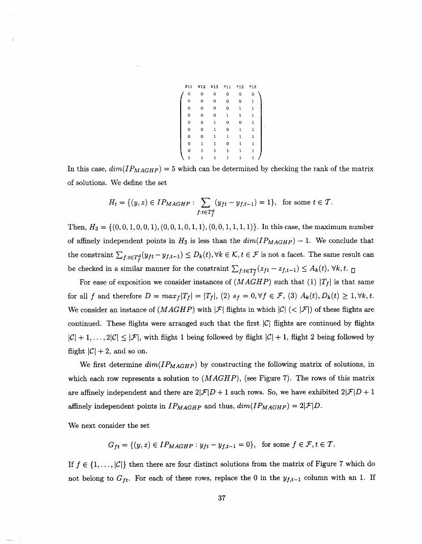
A(t) = 1. Then only the variables y11, Y12, Y13, Z11, Z12, and Z13 are defined. The complete set

of feasible solutions to IPMAGHP is given by:

36

o11

o

0o

o

o

0o

o

o

o

1

In this case, dim(IPMAGHp) = 5 which

of solutions. We define the set

Ht = {(y, z) E IPMAGHP :

Y12 Y13

0 0

0 0

0 0

0 0

0 1

0 1

0 1

1 1

1 1

1 1

can be

Z1 1 Z12 Z13

o o o0

o o 1

o 1 1

1 1 1

o o 1

o 1 1

1 1 1

o0 1 1

1 1 1

1 1 1

determined by checking the rank of the matrix

E (Yft - Yf,t-1) = 1}, for some t E T.f:teTf

Then, H3 = {(0, 0, 1, 0, 0, 1), (0, 0, 1,0, 1, 1), (0, 0, 1, 11, 1)}. In this case, the maximum number

of affinely independent points in H3 is less than the dim(IPMAGHp) - 1. We conclude that

the constraint Zf:tETd(Yft - f,t-1) < Dk(t), Vk E IC, t E is not a facet. The same result can

be checked in a similar manner for the constraint Ef:teT (Zft- zf,t-1) < Ak(t), Vk, t.

For ease of exposition we consider instances of (MAGHP) such that (1) ITfl is that same

for all f and therefore D = maxflTfl = ITfl, (2) sf = 0, Vf E F, (3) Ak(t),Dk(t) > 1, Vk,t.

We consider an instance of (MAGHP) with 1'F1 flights in which CI (< [Fj[) of these flights are

continued. These flights were arranged such that the first ICl flights are continued by flights

ICI + 1,..., 21C I < IFc, with flight 1 being followed by flight ICl + 1, flight 2 being followed by

flight ICI + 2, and so on.

We first determine dim(IPMAGHp) by constructing the following matrix of solutions, in

which each row represents a solution to (MAGHP), (see Figure 7). The rows of this matrix

are affinely independent and there are 21lFlD + 1 such rows. So, we have exhibited 21lFlD + 1

affinely independent points in IPMAGHP and thus, dim(IPMAGHp) = 2IFID.

We next consider the set

Gft = {(y, z) E IPMAGHP: Yft - Yf,t-1 = 0}, for some f E F, t E T.

If f E {1,..., ICl} then there are four distinct solutions from the matrix of Figure 7 which do

not belong to Gft. For each of these rows, replace the 0 in the Yf,t-1 column with an 1. If

37

f E {(ICl+1, ... , 2IC} then there are two distinct solutions from Figure 7 which do not belong to

Gft. For each of these rows, replace the 1 in the Yf,t column with a 0. If f E 21C + 1,..., 1FI}

then there are two unique solutions from Figure (7) which do not belong to Gft. For each

of these rows, replace the 0 in the Yf,t-1 column with a 1. For all of these cases, we have

constructed a matrix with lFID affinely independent rows, proving that dim(Gft) > FiD - 1.

Since Gft is a proper face of IPMIAGHP, we know that dim(Gft) < dim(IPMAGHP). So,

dim(Gft) = IFID - 1 and thus, Gft is a facet of IPMAGHP. o

We next consider the set

Kft = (y, z) E IPMAGHP : Zft - zf,t-1 = 0), for some f E F, t E T.

If f E {1, ... , IC)} then there are three distinct solutions from the matrix of Figure 7 which

do not belong to Gft. For each of these rows, replace the 1 in the Yf,t column with a 0. If

f E {ICI + 1,..., IFI} then there is only one distinct solution from Figure (7) which does not

belong to Gft, so remove this row. For each of these cases, we have constructed a matrix with

IFID affinely independent rows, proving that dim(Kft) > IFID - 1. Since Kft is a proper face

of IPMAGHP, we know that dim(Kft) < dim(IPMAGHP). So, dim(Kft) = IFID - 1 and thus,

Kft is a facet of IPMAGHP-.

We next consider the set

Mt = {(Y, z) E IPMAGHP : Zft - Yf,t-(rf-df) = 0}, for some f E F, t E T.

For all f E {1, ... , i1 } there are t - Tf + 1 distinct solutions from the matrix of Figure 7 which

do not belong to Mft. For each of these rows replace the O's in the columns corresponding to

zft, t < t' < T with l's. Tf and T are the last possible and the earliest possible times that

flight f could arrive, respectively. The remaining matrix will have IFID affinely independent

rows, proving that dim(Mft) > IFID - 1. Since Mft is a proper face of IPMAGHP, we know

that dim(Mft) < dim(IPMAGHP). So, dim(Mft) = IFID - 1 and thus, Mft is a facet of

IPMAGHP-.

Finally, we consider the set

Nf'ft = {(y, z) E IPMAGHP : Yft - Zf't = 0}, for some (f', f) E C, t E T.

38

For all f E { 1,..., F1 } there are t -Tf + 1 distinct solutions from the matrix of Figure 7 which

do not belong to Nf,'ft. For each of these rows replace the O's in the columns corresponding

to yft',t < t' < Tft with l's. The remaining matrix will have l[FID affinely independent rows,

proving that dim(Nfft) > IFID - 1. Since Nf'ft is a proper face of IPMAGHP, we know

that dim(Nfft) < dim(IPMAGHP). So, dim(Nf'ft) = IFID - 1 and thus, Nfft is a facet of

IPMAGHP. O

39

( o o o o 0 -o o o o o 0 o o o o o o 0o 0. 0 o -

O .

* O O

·.

... o _

· .

O .

-·o

... oO .

· -. O O

· ,

. .. o _

.

. .oO O

··+ O

·· 0 4 O

·.. o

·.. o

.. . o

... o

. .. o

·· O

· -O

.. . o

... o

.·. - c

... o

o c

· - O

... o· C

. .'

o o

0 0 --- o

--0 ---

0 0

0 ·- O

0 0 00· . ., . .

0 0 ---0

0 0-.

O a O .. _o

o.- O O

.. ..* .

...

o r o o* ... o

. .o .. o

0' 0 ---

--- --- 00

0 0-- 00

0- 0 -- COO 0 --00

0 0 --- 00

0 - -·-0,

0 - 0··00. ... ...- .

o ·*. .

-0 O --00.. .... .

. ..

0 O-0 O

0 0-··00

0 0 --- 00

0 0-··00..- - -- oo

0 0: : .- ::o

-- -- 00 . ..

0 0--0 .

0 .o o --~ o oo o- o --. ... .o o .· o -

0 0

... o

0 .

o 0

. o

0 0

0 -

..

· .

0 0

o o

0 0.

0 0

.-. o

. .

. 0

0 0

0 0

: -

. o

. o

0.

o

· . o

·- o o

··· 0

O _* ::

... o _

-.. oo

-· O O

·.. o

__O· . .::

·· 0 . O

·-- - O_

-.- c _

Figure 7: Matrix of Solutions to IPMAGHP

40

o0

''- O

..

o0

0 0

0o... 0· .

0 0o 0

0 o0 0

-

. ,

. o...o

L o

4: o

o o

o

o o

4 ::o o

::o

o o

io

a

o o

c

!o

{io

... o

... o

... o

... o

... o

...

... o

·... o

... o

... o

.·.. o

... o

.. o

0 .0 .--

0 - 000 - 00

0 .

0 0 ---00 - 00

0 0 - -

- 0 - -

0 0 --

0 0. .. .

.·

· .

. -.

-: : . :

. .

. .. .

o - o o

O .

o 0 -*

0 - 00

00 --0 a a ·- 0

.

0 0 .. 0

0 0 0'' 0

0 0 ---0 .

0 C0 -- 0

0 0 --- 0o ·- o.... .....

0 0 -- 0.- o

- .-

.

0 0 -*--0.0

0 -- 0· a ··

0 0 ··

·O -- o

·.. .o

O O.. . o-o

'''

... o

... o

·. . oo

·... o· o

·.

-·.o

· .

o

-I

L ·

··· O

· O

0

0

a

0

0

· O

0

0

00

· O

0

0

· O

0

· O

0

a

0

a

a

""

00

References

[1] Andreatta, Giovanni, A. R. Odoni and 0. Richetta (1993), "Models for the Ground-

Holding Problem", chapter in Large-Scale Computation and Information Process-

ing in Air Traffic Control, L. Bianco and A. R. Odoni, editors, Springer-Verlag, Berlin,

1993, pp. 125-168.

[2] Ball, Michael (1993), personal communication.

[3] Garey, Michael R. and Johnson, David S. (1979), Computers and Intractibility: A

Guide to the Theory of NP-Completeness, W.H. Freeman & Company, New York.

[4] Gilbo, Eugene P. (1993), " Airport Capacity: Representation, Estimation, Optimization",

IEEE Transactions on Control Systems Technology, Vol. 1, No. 3, September 1993,

pp. 144-154.

[5] Helme, Marcia (1992), "Reducing Air Traffic Delay in a Space-Time Network", Pro-

ceedings of the 1992 IEEE International Conference on Systems, Man and

Cybernetics, Chicago, pp. 236-242.

[6] Lindsay, Kenneth S., Boyd, E. Andrew, and Burlingame, Rusty (1993), "Traffic Flow

Management Modeling with the Time Assignment Model," MITRE Corporation working

paper.

[7] Nemhauser, George and L. Wolsey (1988), Integer and Combinatorial Optimization,

John Wiley & Sons, New York, pp. 535-572.

[8] Odoni, A. R. (1987), "The Flow Management Problem in Air Traffic Control", Flow

Control of Congested Networks, A.R. Odoni and G. Szego, editors, Springer-Verlag,

Berlin (pp. 269-288).

[9] Richetta, 0. and A. R. Odoni (1993), "Solving Optimally the Static Ground-Holding

Policy Problem in Air Traffic Control", Transportation Science, 27, pp. 228-238.

[10] Richetta, 0. and A. R. Odoni (1994), "Dynamic Solution to the Ground-Holding Policy

Problem in Air Traffic Control", to appear in Transportation Research.

41

[11] Terrab, M. and A. R. Odoni (1993), "Strategic Flow Control on an Air Traffic Network".

Operations Research, pp. 138-152.

[12] Terrab, M. and Paulose, S. (1993), "Dynamic Strategic and Tactical Air Traffic Flow

Control", RPI Technical Report.

[13] Vranas, P., D. Bertsimas and A. R. Odoni (1994a), "The Multi-Airport Ground-Holding

Problem in Air Traffic Control", Operations Research, pp. 249-261.

[14] Vranas, P., D. Bertsimas and A. R. Odoni (1994b), "Dynamic Ground-Holding Policies

for a Network of Airports", to appear in Transportation Science.

42