The Adequacy of Investment Choices Offered

By 401K Plans

Edwin J. Elton*

Martin J. Gruber*

Christopher R. Blake**

* Nomora Professors of Finance, New York University ** Professor of Finance, Fordham University

The Adequacy of Investment Choices Offered by 401K Plans

Abstract

Defined-contribution plans represent a major organizational form for investors’

retirement savings. Today more than one third of all workers are enrolled in 401K plans. In a

401K plan, participants select assets from a set of choices designated by an employer. For over

half of 401K-plan participants, retirement savings represent their sole financial asset. Yet to date

there has been no study of the adequacy of the choices offered by 401K plans. This paper

analyzes the adequacy and characteristics of the choices offered to 401K-plan participants for

over 400 plans. We find that, for 62% of the plans, the types of choices offered are inadequate,

and that over a 20-year period this makes a difference in terminal wealth of over 300%. We find

that funds included in the plans are riskier than the general population of funds in the same

categories. We study the characteristics of plans that are associated with adequate investment

choices, including an analysis of the use of company stock, plan size, and the use of outside

consultants. When we examine one category of investment choices, S&P 500 index funds, we

find that the index funds chosen by 401K-plan administrators are on average inferior to the S&P

500 index funds selected by the aggregate of all investors.

Keywords: 401K plans, pension, spanning, portfolio, investment choices

JEL classification: G11, G12, G23, E21

A major trend in pension plans offered by companies is a movement from defined-benefit

plans to defined-contribution plans. The majority of defined-contribution plans offered by

companies are 401K plans. More than one third of all workers are enrolled in 401K plans, and

these plans have over one trillion dollars under management. There has been some research on

how investors react given the investment choices they face. For example, investors tend to

allocate their funds equally over the investments they are offered. This is often referred to as the

“1/n Rule” (see Benartzi and Thaler (2001) and Liang and Weisbenner (2002)). Another finding

is that investors over-invest in stock of the company for which they work (see Huberman and

Sengmuller (2003) and Agnew and Balduzzi (2002)).

With all the interest in how investors react given the choices they are offered, it is

surprising that there have been no studies of the appropriateness of the decisions that

corporations make with respect to which investment choices to offer plan participants. The

investment alternatives offered are important to participants because, for over one half of plan

participants, the 401K investments are their sole financial assets. Even for those participants who

hold other financial assets, the 401K assets are likely to be the bulk of their financial assets, so

that plan offerings are likely to restrict the portfolios they can hold.

What choices should a corporation offer to plan participants? For those participants for

whom 401K investments are their sole financial assets, the corporation should offer a sufficient

set of investment alternatives so that the investor could construct the same efficient frontier that

he or she would obtain if there were choices from a reasonable set of alternatives. Investors who

have other financial assets would not be hurt by such a strategy, so this strategy is dominant for

all investors.1 In this paper we examine the adequacy of the investment alternatives offered by

401K plans utilizing mutual funds.

This paper is divided into eight sections. In the first section we discuss the data used. In

the second section we discuss two ways of classifying investment choices to form alternative

portfolios to compare against actual 401K plan offerings, and we explore which type of

classification offers the best set of alternative choices for plan participants. In the third section

we examine the minimum number and types of alternative investment choices to include in the

optimal choice set of the comparison portfolios. In the fourth section we examine whether or not

the mutual funds offered would suggest that 401K plan administrators consider risk in deciding

which investment choices to offer. In the fifth section we explore issues of how well the fund

offerings span the efficient set. In that section, we not only examine statistical tests, but we also

examine economic significance (effect on participants’ returns) of a failure to provide

appropriate offerings. In the sixth section we examine the effect of offering company stock on

plan risk and the efficient frontier. In section seven we examine whether other characteristics of

the plans affect the appropriateness of the investment choices offered to plan participants.

Finally, in section eight we summarize our results.

I. Data

Our data were provided by Moody’s Investor Services. Moody’s collects data by means

of a survey of pension plans offered by both for-profit and non-profit entities (collected in 2002

with information through 2001). From this data set we selected all 401K plans that employed

publicly available mutual funds for participant choices. However, we did not exclude plans that

1 If a plan is administered by an external party, the administrator may charge additional fees if the company wishes to include funds outside the external party’s normal offerings. However, there are so many plan

offered, in addition to mutual funds, non-public money market funds, GICs and stable value

funds and/or company stock. We were able to identify 680 401K plans for which the CRSP

mutual fund database contained at least some data on each of the mutual funds offered in the

plan. Of the 680 plans, 417 had at least five years of total returns data in the CRSP database for

every mutual fund they offered.2 For each of these plans we collected data on the mutual funds

offered, historical returns for each mutual fund, and the names and characteristics of the firms

offering the plans.

Table 1 shows the number of distinct investment choices offered by the 680 plans

mentioned above. The median number of 401K plan offerings is eight. Approximately 12% of

the 401K plans offer four or fewer investment choices, and approximately 11% offer 13 or more

investment alternatives. The median number of investment offerings we report is somewhat less

than that reported by Huberman and Sengmuller (2003). Huberman and Sengmuller’s data

sample came from 401K plans managed by Vanguard. Many plans restrict their offerings to one

fund family. Vanguard is one of the largest mutual fund families in terms of number of funds

offered. Thus it is not surprising, and is consistent with what we observed in our sample, that

plans managed by Vanguard offer more choices than would be observed in the population.

Table 2 shows the percentage of plans that offer various types (using ICDI

classifications) of investment choices to their participants. The most common investment choice

(offered by 97.4% of plans) is a domestic equity fund. The next most common offering (86.8%)

is an alternative such as a GIC or money market fund, where interest is intended to be the only

source of return. Other common offerings fall in the following categories: domestic bond funds

administrators for a company to choose from that this is unlikely to have an effect on our findings. 2 When later we draw general samples of mutual funds for comparison purposes, we use the same selection procedure so that comparisons are not biased.

(71.5%), domestic mixed bond and stock funds (80.6%), and international bond and/or stock

funds (75.1%). The high percentage of 401K plans that offer international funds is surprising,

given the much lower percentage international funds constitute of mutual funds publicly

available to investors. Finally, 22.9% of the 401K plans offer company stock as an alternative for

their participants.

Forty-eight of the 680 plans offered pension participants at least one specialized fund as

an alternative choice; there were a total of 56 such choices. Thirty-one of these specialized funds

were science and technology funds, six were real estate funds, five were telecommunications

funds, four were healthcare funds, four were natural resources funds, four were utilities funds,

one was an e-commerce fund and one was a financial services fund. There is no relationship

between type of specialized funds offered and the type of firm offering the 401K plan. We noted

that 33 of the 56 specialized funds were T. Rowe Price funds, suggesting that recommending

inclusion of a specialized fund is a strategy employed to market T. Rowe Price funds to 401K

plan administrators. The large number of science and technology funds offered at the date our

sample was constructed suggests that some plan administrators were including the then-current

“hot” sector.

II. Determining the Comparison Portfolios

In order to determine if 401K plans offer their participants adequate investment choices,

we need to hypothesize an adequate set of alternative investment choices. There are two

approaches we can use to determine an adequate set of alternative investment choices. The first

approach draws on the field of financial economics, where extensive literature exists that

discusses indexes that are necessary and sufficient to capture the relevant return characteristics

for a range of investment choices. The second approach draws on the development by the

financial industry of a set of classifications that the industry finds relevant for classifying

investment portfolios. These classifications represent the investment industry’s attempt to

separate mutual funds into groups that behave similarly and define a complete set of relevant

investment choices. In this section of the paper we examine both of these methods for classifying

investments to see which classification provides a better set of alternative investment choices.

Initially, we examine classifications from research on what affects returns. For common

stocks, we classified by value versus growth and by size as advocated by Fama and French

(1994). Because of industry practice, we classified by size into three groups: small-cap, mid-cap

and large-cap. Each of these three groups was then further divided into value and growth.3 All

six indexes were taken from Wilshire. We chose Wilshire indexes because there are existing

tradeable funds that attempt to match them. For bonds, we used a general bond index, including

governments and corporates, a mortgage-backed index, and a high-yield index. This division is

supported by Blake, Elton and Gruber (1993), who found this division was sufficient to capture

differences in return across bond funds. We used the Lehman U.S. Government/Credit index for

the general bond index, the Lehman Fixed-Rate Mortgage-Backed Securities index for the

mortgage index, and the Credit Suisse First Boston High-Yield index for the high-yield bond

index. We also included the Salomon Non-U.S.-Dollar World Government Bond index for

international bonds and the MSCI EAFE index for international stocks.4

3 This division is also supported by Elton, Gruber and Blake (1999), who found that these indexes plus a bond and international index captured most of the return differences among funds. 4 We also considered adding a real estate index. However, only six of our 417 sample 401K plans include a real estate fund. Therefore, we dropped real estate when we looked at sufficiency of offerings of 401K plans, so that rejection of sufficiency of any sample 401K plan’s offerings would not be due to the exclusion of a real estate investment choice. However, we should note that inclusion of a real estate index did improve the efficient frontier in some periods.

Since returns on all mutual funds are computed after expenses, we deducted expenses

from each of our indexes. For each of our indexes, we used the expense charge of the index fund

(including exchange-traded funds) that most closely matched the index. If there were multiple

index funds matching the index, we used the expense charge of the lowest cost fund. In what

follows we refer to these indexes as “Research-Based” indexes, or “RB” indexes.

The second method for selecting categories of funds that might be appropriate to include

in 401K plans is to use one of the public investment services’ fund classifications based on fund

objectives and policies. These classifications represent the investment industry’s attempt to

divide funds into groups that behave similarly and are a complete set of investment alternatives.

Groups based on ICDI classifications and the percentages of plans that offer any particular group

to a participant are shown in Table 2. For each ICDI investment objective group except interest-

only funds and utility funds, we computed a monthly return index starting in January 1992 and

ending December 2001 (10 years) by taking an equally weighted average each month of the

returns on all funds in the group that existed as of January 1992. If, during the 10-year period, a

fund ceased to exist or changed objectives, the fund was dropped from the index at that point in

time.5 In what follows we will refer to these indexes as “Objective and Policy-Based” indexes, or

“OPB” indexes.

In the next section, we compute Sharpe ratios and perform intersection tests to examine

which of these classifications provide better opportunities for investors.

5 The CRSP mutual fund database is not very accurate in properly recording when a firm ceased to exist or changed objective. Elton, Gruber and Blake (2001) showed this does not add bias. The way we constructed each index assumes investors reallocate their money across the remaining funds in the group when a fund changes objectives or ceases to exist.

II.A. Sharpe Ratios

Table 3 shows the Sharpe ratios for optimal portfolios when short sales are not allowed

constructed from the 11 RB indexes and the 14 OPB indexes for the ten-year period 1992-2001

and the two five-year sub-periods.6 In computing Sharpe ratios we used as the risk-free rate the

average of the 30-day CRSP T-bill rate over the relevant period. In the two five-year sub-periods

and in the 10-year period the Sharpe ratios are higher for the efficient frontier calculated using

returns on the RB indexes. Furthermore, the differences in Sharpe ratios between the two sets of

indexes are statistically significant in both of the five-year subperiods. (The significance tests are

described in Appendix A.)

The evidence in Table 3 indicates that classifying funds along the lines suggested by the

literature of financial economics may be superior to accepting commonly used objective and

policy classifications such as those provided by ICDI. Next we will examine intersection tests to

see what this adds to the analysis.

II.B. Intersection Tests

One of the principal tests used in this paper is a test of intersection, a particular form of

spanning. For example, if a set of choices were offered to holders of a 401K plan, do these

choices lead to the same efficient frontier as would a more general set of options? Spanning is

important because for over half the 401K participants the 401K investments are their sole

financial investments. Tests of spanning are discussed in Huberman and Kandel (1987), De

Santis (1994), Bekaert and Urias (1996) and DeRoon, Nijman and Werker (2001), among others.

In this article we make use of the results derived in DeRoon et al (2001) for the case of short

sales disallowed. At this point we will provide an intuitive explanation for the methodology used

both in this section and in later sections of this paper, followed by an application of the

methodology to RB and OPB indexes.

II.B.1. Methodology

The purpose of the intersection test is to examine whether, given a riskless rate, a

particular set of benchmark assets is sufficient to generate the efficient frontier or whether

including (long or possibly short) members of a second set of assets would improve the efficient

frontier at a statistically significant level.

As DeRoon et al (2001) have shown, if the optimal (tangent) portfolio consists of K

benchmark assets, then intersection is a test of the impact of restricting the intercept (α) in the

following time-series model:

( ) itfBkt

K

kikifit RRRR εβα +−+=− ∑

=1 (1)

where

itR = the return on non-benchmark asset i (i = 1, …, N) in month t;

fR = the risk-free rate;

BktR = the return on benchmark asset k in month t;

itε = the error term for asset i in month t.

When short sales are allowed, intersection occurs if, for all of the N non-benchmark

assets jointly, the iα are not statistically significantly different from zero, i.e., the restrictions are

0=iα ∀ i (1a)

6 Throughout this paper, the case of short sales not allowed is emphasized because a plan’s participants can not short sell the mutual funds offered by the plan.

When short sales are not allowed, the right-hand side of equation (1) includes returns on

only those benchmark assets that are held long in the optimal portfolio of benchmark assets.7

Intersection occurs if, for all of the N non-benchmark assets jointly, the iα are not statistically

significantly positive, i.e., the restrictions are

0≤iα ∀ i (1b)

The logic behind the test can be easily understood. In the case of short sales allowed if an

asset had a positive (or a negative) alpha, then including the asset long (or short) would improve

the efficient frontier. Without short sales, only the inclusion of an asset with a positive alpha

would improve the efficient frontier.

To test whether, given a riskless rate, we have a set of benchmark assets that spans the

relevant space, we simply have to test the unrestricted model (equation (1)) against the model

with the restrictions on alpha. This involves employing equation (1) using the restrictions (1a)

( 0=iα ∀ i) for the case where short sales are allowed and using the restrictions (1b) ( 0≤iα ∀

i) for the case where they are not allowed.

To test whether or not the restrictions hold, we use the likelihood ratio test statistic

suggested by Gallant (1987) with small-sample adjustment. The likelihood ratio test is:

( )|ˆ|ln|~|ln Σ−Σ= TL (2)

where T is the number of time-series observations, Σ~ is the estimated variance-covariance matrix

of the residual errors of the N non-benchmark assets from the restricted equation, and Σ̂ is the

estimated variance-covariance matrix of the residual errors of the N non-benchmark assets from

the unrestricted equation. L is asymptotically distributed as chi-squared with q degrees of

7 These benchmark assets can be easily identified by solving a quadratic programming problem.

freedom, where q is the number of parametric restrictions. For small samples such as we have

cross-sectionally, Gallant recommends the use of the F distribution with degree-of-freedom

corrections instead of the chi-squared distribution. The small-sample adjustment is simply to

compare L to , where is the F statistic at significance level x with q numerator degrees

of freedom and T × M – p denominator degrees of freedom, and where M is the number of

equations estimated and p is the number of parameters. If L is greater than , then the null

hypothesis that the restrictions hold is rejected.

xFq × xF

xFq ×

II.B.2. Results

Since Sharpe ratios suggest that RB indexes are potentially superior to OPB indexes, we

examine the following question: if we construct the efficient frontier using RB indexes, does

adding OPB indexes shift the efficient frontier?

When we do not allow short sales, the answer is the same in each five-year subperiod and

in the overall ten-year period. We can not reject the hypothesis that the intercepts are zero or less

for the OPB Index, which implies that adding OPB Indexes does not shift the efficient frontier.

In fact, in the ten-year period and both five-year subperiods, the determinants of the constrained

and unconstrained variance-covariance matrices of the residuals are the same.

When short sales are allowed, adding the OPB Index causes the efficient frontier to shift

and we reject the hypothesis that the intercepts are zero. However, examining the individual

intercepts reveals an interesting pattern. In the ten-year period and both five-year subperiods, all

intercepts from the unrestricted model are negative in the case where short sales are not allowed.

This means that the efficient frontier shifts because we short-sell the OPB indexes. Since short

sales are not allowed for 401K plans, none of the OPB indexes improves the choice set. The

universally negative intercepts also explain why the determinants of the constrained and

unconstrained variance-covariance matrices of the residuals are the same. The constraint that the

intercepts are non-positive is not binding.

The intersection tests show that none of the OPB indexes improve optimal portfolios

derived from RB indexes when short sales are not allowed. In addition, the Sharpe ratio tests

tend to support the conclusion that RB indexes provide a better set of alternatives. Thus, in what

follows we will use the categorization suggested by financial research. This set of choices works

at least as well as the set of choices that the investment community accepts as sufficient to

delineate the relevant choice set for investors.

III. Reducing the Number of Choices

Having determined that the categorization from financial research is no worse and

probably better than commonly used objective and policy classifications, the next question to ask

is whether some of the RB index classifications are redundant and, if so, what is the composition

of the reduced set. We want to exclude redundant indexes from our index set, because their

inclusion might result in our rejection of the adequacy of the investment choices offered by some

plans purely on the basis of chance. We examine reducing the set of indexes in three ways:

composition of efficient frontiers, factor analysis, and cluster analysis. We present the details of

the analyses in Appendix B, and we summarize the results below.

We first examined composition of the efficient portfolio for each of 12 time periods.

Some categories (e.g., mid-cap growth stocks) never entered the efficient frontier, while others

(e.g., mid-cap value and small-cap value) occasionally entered and often substituted for each

other.

We next performed maximum-likelihood factor analysis on the data. Using several tests

for statistical significance, a five-factor solution was indicated. Rotating the five factors (using

quartimax rotation) allowed us to associate economic characteristics with each of the five factors.

However, two of the factors involved a positive weight on one index and a negative weight on a

second index (e.g., a positive weight on the growth index and a negative weight on the value

index), and, since pension funds can not short sell securities, replicating the five factors requires

at least seven of our original 11 indexes.

As a final step, cluster analysis was performed on the 11 RB indexes. The results

indicated 8 identifiable groups. From the analysis, three pairs of the 11 RB indexes were

combined (small-cap growth with mid-cap growth, small-cap value with mid-cap value, and

government/corporate bond with mortgage bond), leaving us with a final set of 8 RB indexes.

IV. Diversification of 401K Plan Offerings

In this section we examine the extent to which 401K plan administrators consider risk

when they decide on which investment choices to offer plan participants. To examine this, we

compare the risk of the actual 401K plan offerings to the risk of offerings from “synthetic” 401K

plans constructed by using random selection of publicly available mutual funds. We have several

ways to implement this random selection. The simplest, and most direct, method is to make the

odds of selecting a fund from any ICDI category equal to the proportion of that category held by

our sample of 401K plans. Within a category (e.g., aggressive growth) the odds of choosing any

single fund are made equal. The population of funds from which we select consists of all funds

that exist as of the end of 2001 and have five years of history. These are the same criteria we

used when selecting 401K plans to include in our total returns sample.

This is an extremely naïve selection rule that ignores completely the correlation between

ICDI categories. A slightly less naïve strategy would force all synthetic plans to hold at least one

randomly selected bond fund and one randomly selected stock fund. Examining the holdings of

the actual 401K plans shows that this is a strategy followed by many plans. Thus our second

random-selection strategy, called “constrained random selection,” follows the same random-

selection rules described above except that all synthetic plans are forced to hold at least one bond

and one stock fund.

To calculate portfolio variances for both the actual 401K plans and the synthetic 401K

plans, we need to formulate a rule to represent the investment weighting for a hypothetical plan

participant. Given the strong evidence that plan participants equally weight their 401K plan

offerings (see Benartzi and Thaler (2001) and Liang and Weisbenner (2002)), we use one

divided by the number of a plan’s investment choices to represent a participant’s chosen

investment weight in each of the plan’s mutual fund offerings.8

While estimates of variances and covariances differ according to the random-selection

rules we use, we can compute overall synthetic plan portfolio variance for each random-selection

rule using the standard formula for an equally weighted portfolio.9 The portfolio variance is:

CovN

NVarN

VarPN ×⎟⎠⎞

⎜⎝⎛ −

+×⎟⎠⎞

⎜⎝⎛=

11 (3)

where NVarP is the average variance of a portfolio consisting of N funds drawn at random from

our population of mutual funds, with equal investment in each fund selected, and Var and Cov

are the average fund variance and the average covariance between funds, respectively, if funds

8 We exclude from the investment choice sets company stock, GICs, stable value funds and money market funds.

are selected using either of the random selection techniques discussed earlier. (For details on

how Var and Cov are calculated, see Appendix C.)

Table 4 presents the average values (by number of funds offered) of the variances for the

actual 401K plans as well as the variances that would occur if plan sponsors selected funds at

random using either of the selection rules described above.10 The first thing to note from Table 4

is that, while on average the variance of return on actual 401K plans is lower than the variance

would have been if plan sponsors had randomly selected a set of mutual funds, it is higher once

we make the realistic assumption that the synthetic plans have at least one bond fund and one

stock fund. Plans on average have a variance that is 2.29 lower than that using random selection

of funds but 2.087 higher than that using constrained random selection.11 Both differences are

statistically significant at better than the 0.01 level. It is also interesting to note that as plans offer

more investment choices (beyond three) the overall risk is reasonably flat

To gain more insight into the risk of 401K plans, we separately examined the average

variance of individual funds held by all plans and the average correlations between the funds

held by all 401K plans. The average individual variance of the mutual funds held by 401K is

26.76. If 401K plan sponsors selected mutual funds randomly but maintained the same

percentage in each ICDI category as the aggregate of all plans, the average fund variance would

have been 30.49. If instead we simply computed an average fund variance across all mutual

funds, weighting each fund equally, the variance would be 31.26. Thus 401K plan administrators

9 See Elton and Gruber (1977). 10 Only one of our 417 sample 401K plans offered 17 funds; therefore we do not report average values for 17-fund plans in Table 4. 11 Because average variances can not be constructed using constrained random selection for plans with only 1 fund, the reported averages and significance tests exclude the 10 401K plans in our sample that offered only 1 fund (along with the one plan that offered 17 funds) for a total of 406 funds.

select mutual funds with a lower fund variance both relative to what it would be if they randomly

selected funds while maintaining the aggregate plan proportions in ICDI categories and relative

to what it would be if they simply randomly selected across all available funds.

The other element that affects portfolio variance is correlation. The average pairwise

correlation among funds selected by 401K plans is 0.60, while for random selection, maintaining

ICDI proportions, it is 0.55. The difference is statistically different at the 1% level. Thus plan

administrators select funds that are more highly correlated than the average correlation between

pairs of funds.

Overall, plan administrators offer plan participants mutual funds with less variance than

randomly selected funds, but funds that are more highly correlated. Managers appear to pay more

attention to a fund’s variance than to the correlation of the fund with other plan choices when

selecting funds. For plan participants using the 1/n Rule, this results in lower variance than pure

random selection. However, it results in a much higher variance than random selection if all

random portfolios are constrained to include at least one bond and one stock fund.12

V. Adequacy of Plan Offerings

In looking at the adequacy of plan offerings, we have to look beyond the risk attributes

discussed above, since return as well as risk affects the efficient frontier. In this section we use

spanning tests to see if plans offer participants adequate investment choices.

Earlier we argued that an investor could be satisfied with a choice from among eight

research-based indexes. The question is whether the choices offered by 401K plans span the

12 The random selection leads to more small funds being selected than 401K plans actually hold. If we control for this by eliminating funds less than $50 million in size, the variance of randomly selected funds is reduced to 29.592 if we maintain the same percentage in each ICDI category as funds selected, or 30.726 using equal probability of selection for all funds.

space delineated by the eight RB indexes; if they do not, then optimal investment choices are not

being offered. Since plan participants can not short sell assets in their 401K plans, we use the

intersection test described earlier for the case where short sales are not allowed. The results of

the intersection tests are shown in Table 5.13 Plans holding four or fewer funds rarely offer a set

of funds that span the eight RB indexes. For these plans there are more RB indexes than fund

offerings. However, it is possible that a small set of funds spans the larger set of RB indexes,

either because some of the RB indexes are not desirable investments or because some of the

funds are combinations of two or more of the RB indexes. However, this does not happen for

funds offering a small set of investment choices. For plans holding seven or more funds, we find

that about 54% of the plans offer investment choices that span the relevant space investors are

interested in.14 Of course, the glass is also half empty in that 46% of the plans leave investors

unsatisfied. Finally, it is not until plans offer 14 or more investment choices (4.2% of all plans)

that virtually all plans offer investment choices that span the space investors should be interested

in.

Of the 406 plans, only 38% span the space obtainable from the eight RB indexes.15 While

some 401K plans offer participants a rich enough selection of investment choices to satisfy their

needs, clearly a number of 401K plans do not do so.16

13 The results in Table 5 exclude the same 11 plans excluded in Table 4, leaving a total of 406 plans. 14 The sample of 417 plans was constructed to include only those 401K plans where all offerings had five years of history. The distribution of the number of offerings with that restriction differs from the distribution of the number of offerings by 401K plans in general. If we apply the distribution of “yes” and “no” shown in Table 5 to the distribution of investment choices shown in Table 1 and assume that all plans with 17 or more investment choices span, the percentage rises to 58%. 15 For the reasons discussed in the prior footnote, we apply the distribution of “yes” and “no” shown in Table 5 to the distribution of investment choices shown in Table 1, counting each plan offering one investment choice as a “no” and each plan offering 17 or more investment choices as a “yes.” Applying these rules, the percentage of plans that span is 40%.

Before leaving this section, it is worthwhile examining the loss in return to 401K plan

holders due to plans not spanning the relevant space. For the 406 plans in our sample to have the

same Sharpe ratio as a portfolio comprised of the 8 RB indexes, the average return on the plans

would have to increase by 1.81% per year. For the 249 plans that do not span the space, average

return would have to increase by 3.16% per year to match the Sharpe ratio on the 8 RB indexes.

The 3.16% increase in return is equal to 42% of the return on the 8-RB-index portfolio. Thus,

investors in 401K plans are sacrificing significant return because plan administrators are offering

an incomplete set of investment alternatives.17

It is interesting to note why these differences in return occurred. The bulk of the

differences in Sharpe ratios occurred because the plans had much more risk than a portfolio

comprised of the 8 RB indexes. The problem lies not in plans selecting individual mutual funds

that perform badly, but rather in plans offering too few investment choices, choices with high

risk, and choices that are too highly correlated.

Our sample does not allow us to do a detailed analysis of the appropriateness of the

choice of individual funds in each category of funds offered in the plans. There is not enough

data after our sample ends (2001) to do a meaningful analysis of subsequent performance, and, if

we used returns prior to 2001 for analysis, we would have serious selection bias. However there

is one type of fund for which we can analyze the reasonableness of the plan administrators’

choices: S&P 500 index funds. As Elton, Gruber and Busse (2003) have shown for this type of

16 As a further check on plans spanning, we considered whether plans spanned the space of the simplest set of choices we could think of: a broad stock market index (the Wilshire 5000 index), a bond market index (the Lehman U.S. Government/Credit index), and an international index (the MSCI EAFE index). We adjusted the returns of the 3 indexes to reflect normal management fees (just as we did for the 8 RB indexes). With this limited set of 3 indexes, more plans offered choices that spanned the indexes’ space. However, 42 of the 406 plans still did not span, and over half of those plans offered 6 or more choices. 17 These differences are much larger than any possible differences due to expense ratios. See Elton, Gruber and Blake (1996) for estimates of expense ratios.

fund, future relative performance can be predicted with a high degree of accuracy by using the

funds’ expense ratios. Since S&P 500 index funds all hold virtually the same stocks in the same

proportions, differences in performance are almost identical to differences in expense ratios. We

ranked the S&P 500 index funds in the Elton, Gruber and Busse sample by expense ratios and

divided them into low annual expense ratios (0.06% to 0.36%) and high annual expense ratios

(0.37% to 1.36%). Of the money invested in their sample’s S&P 500 index funds by all investors

in 2001, 11.16% is invested in high-expense funds. In our sample of 417 401K plans, 180 plans

offered S&P 500 index funds. 21.55% of the S&P 500 index funds offered to participants by the

plan administrators are in the high-expense category. This is considerably more than would be

invested if the plan administrators’ investment pattern were the same as the aggregate of all

investors. Thus, for S&P 500 index funds, plan administrators as a group make poorer choices

than the average investor.

VI. Company Stock

The analysis to this point has ignored company stock as an asset in 401K plan offerings.

In this section we explore the impact of including a firm’s own stock as one of the investment

choices in the 401K plan. We examine the impact of including company stock on the plan risk,

Sharpe ratio, and likelihood of spanning.

On average, companies offering company stock as an investment choice offer the same

number of mutual fund choices as those that do not offer stock; therefore, companies offering

company stock do not offer plan participants fewer fund choices as a mechanism to encourage

participants to hold more company stock.

To examine the effect of company stock on overall risk, we took all plans that offered

company stock as an investment choice for which stock returns existed over our five-year period.

For these plans we computed the variance using data for the last five years of an equally

weighted portfolio of all offerings, with and without the company stock. For the companies

offering company stock, when the company stock was included, the variance of the portfolio of

401K offerings using the 1/n Rule went up by 3.17. Of the 55 plans for which we have data, 36

have a higher variance when company stock is included in the portfolio. The 3.17 increase in

variance associated with including company stock is a percentage increase of about 19%, and

using a one-tailed pairwise t-test, this increase is statistically significant at the 1% level (t = 3.6).

Although the inclusion of company stock leads to risk increasing, Sharpe ratios might

also increase. To examine this we examined the Sharpe ratios for optimal portfolios with no short

sales. When company stock was not allowed to enter the optimal portfolio, the average Sharpe

ratio was 0.240. When company stock was allowed to enter, the Sharpe ratio increased slightly to

0.255. Remember that including more securities in the population will in general increase the

Sharpe ratio. If we control for this by comparing the increase from including company stock with

the increase from including a randomly selected mutual fund, the difference is close to zero and

is neither statistically significant nor economically significant. This is true despite the fact that

company stock enters the optimal portfolio in 26 out of 55 cases.

The most important test of the impact of company stock is the spanning test. Does

including company stock increase the number of 401K plans that have offerings that span the

space of our eight RB indexes? The data show that whether company stock is included in the

choice set or not, there is no change in the number or identity of the plans for which spanning

takes place.

In summary, the inclusion of company stock causes an increase in risk. However, this is

more than offset by an increase in return, resulting in a very slight improvement in the Sharpe

ratio. However, the increase in the Sharpe ratio is about the same as it would be if we randomly

included an additional mutual fund rather than the common stock. The inclusion of company

stock doesn’t change the set of plans that span the space of the RB indexes. Considering the

401K plan as the participant’s sole financial asset, the inclusion of company stock in a plan

seems to neither improve nor harm the investor making intelligent 401K plan choices. However,

since a plan participant’s labor income may be highly correlated with the performance of the

company stock, a portfolio including labor income, 401K mutual funds and the company stock

may be significantly more risky than a portfolio excluding the company stock.

VII. Plan Characteristics

In this section of the paper we examine the relationship between plan characteristics and

performance. Before we turn to performance per se, we want to examine one characteristic of

plans that seems to have a major impact on how management behaves and which serves as a

parameter that might affect performance.

In Table 6 we divide all plans by the size of assets invested in each plan into 10 deciles.18

The average size of the plan in each decile is shown in the second column. There is a wide

variation in plan size, with the average plan in the tenth decile over 300 times as large as the

average plan in the first decile. The first question we examine is whether plans with more assets

under management offer participants more investment choices. As shown in Table 6, there is a

clear and statistically significant relationship (at the 1% level) between plan size and the number

of investment choices offered. Since from our spanning tests we know that more investment

choices are generally better for investors, this suggests that large plans ceteris paribus offer an

advantage to the 401K participants.

Are companies that manage large plans more sophisticated than companies that manage

small plans? In particular, are companies with large 401K plans more likely to hire outside

consultants and use sophisticated strategies such as utilizing futures and options, hedging

strategies and quantitative methods? As shown in Table 6, a higher percentage of larger plans

hire outside consultants and engage in more sophisticated investment strategies. The relationship

of both with size is statistically significant at the 1% level in both cases.

We next examine the relationship between size and whether a plan votes proxies in the

companies it owns. Proxy voting can be interpreted as either another measure of sophistication or

as a measure of social consciousness. We find at best a weak positive relationship, one that is not

statistically significant.

Finally, we examine the relationship between the size of plan assets and the probability of

a company including its own stock in its 401K plan. Not surprisingly, large plans show a

stronger tendency to include company stock in the plan than do small plans, and this relationship

is significant at the 1% level.

Next we examine whether the use of outside consultants or sophisticated strategies

improves the position of plan participants. To do so we examine their impact on number of plan

investment choices, optimal Sharpe ratios and spanning.

It is clear from Table 6 that there is an association between average plan size and both the

employment of outside consultants and the use of sophisticated investment tools. It is also clear

18 We were unable to obtain plan size data for 28 of the 417 tracked funds; the size deciles were formed using the remaining 389 plans.

that larger sized plans have more investment choices. Therefore, if we want to discover whether

employing outside consultants or using sophisticated strategies leads to more investment choices

per se we need to control for plan size. We divided all plans into two groups based on whether or

not they employed outside consultants and two groups based on whether or not they used

sophisticated strategies. For each plan in the group we calculated the difference between the

number of investment choices the plan actually offered and the number of investment choices we

would expect given the plan’s size. We then computed the average difference for the group

employing outside consultants (or sophisticated strategies) and the group that did not. The

significance of this difference was then tested using a standard t-test. Although the sign was as

expected, the relationship between the number of investment choices and the use of outside

consultants or sophisticated strategies was not statistically significant at meaningful levels of

significance.

The other issues we would like to examine are whether employing outside consultants or

sophisticated strategies leads to better Sharpe ratios or a greater likelihood of the investment

choices offered spanning the investment space. From portfolio theory we know that the greater

the number of investment choices offered ceteris paribus, the higher the average Sharpe ratio

and the more likely the offerings will span the space. Thus, to examine this question we need to

control for number of investment choices. We divided the plans into two groups based on

whether or not they employed consultants, and two groups based on whether they used

sophisticated strategies. Within each group, given the number of investment choices offered, we

computed the differences in actual Sharpe ratios and expected Sharpe ratios as well as

differences in actual proportions that span and expected proportions that span. We then

compared these differences between the group that employed outside consultants and the group

that did not and the differences between the group that employed sophisticated strategies and the

group that did not. For each case, the difference, while in the expected direction, was not

statistically significant. Thus there is at best weak evidence that plans that use outside

consultants or sophisticated strategies offer more investment choices, have higher Sharpe ratios,

or better span the space.

VIII. Conclusion

In this paper we examine the reasonableness of the investment choices offered by 401K

plans. In order to analyze this we need to determine a group of investment vehicles that plan

participants would find attractive. We consider two alternatives: designing a portfolio that

represents each of the standard classifications used by the financial industry and designing a

portfolio that represents each classification suggested by the literature of financial economics.

Employing factor analysis, cluster analysis, Sharpe ratios and spanning tests, we conclude that

eight portfolios based on the literature of financial economics representing large-cap growth,

small- and medium-cap growth, large-cap value, small- and medium-cap value,

government/corporate/mortgage-backed debt, international equity, non-U.S. world bond and

high-yield debt successfully span the space described by the larger set of indexes employed by

the financial community. These eight indexes (called RB indexes for research-based indexes) are

used as benchmarks in the latter part of the paper.

The second part of the paper examines the investment choices offered by 401K plans. We

first examine risk. We find that 401K plans have slightly less risk than randomly selecting funds

where the percentage of funds that is randomly selected from any ICDI classification is the same

as the aggregate of all plans. However, if a plan sponsor used a common-sense rule of insisting

that the plan include at least one stock and one bond fund, then plan risk from random selection

would be smaller than the actual risk of the 401K plans. Although the individual funds selected

by 401K plans have lower variance than randomly selected funds, the correlation between them

is higher.

However, risk is only part of the story of what happens to overall performance. How

adequate are plan offerings? Here we use spanning tests to see if the plan offerings span the

space offered by the eight RB indexes. Only 38% of 417 plans span the space defined by the

eight RB indexes. This means that, for 62% of the plans, the plan participants would be better off

with additional investment choices. In fact, if these plans spanned the 8 RB indexes, participants’

average return would improve by 3.2% per year, which is 42% of the return on an 8-index

portfolio with the same level of risk. While significant on a 1-year basis, over a 20-year period (a

reasonable investment horizon for a plan participant), the cost of not offering sufficient choices

makes a difference in terminal wealth of over 300%. Since, for more than one half of plan

participants, a 401K plan represents the participant’s sole financial asset, the consequences are

serious.

We then examine plan characteristics to see if they can add insight into the adequacy of

plan investment choices. We first examine plan size. There is a strong correlation between the

number of investment choices a plan offers and size. This is a strong indication that participants

in larger plans are better off than participants in smaller plans. In addition, larger plans are more

likely to use outside consultants and to include more sophisticated strategies in the plan. This

raises the question of whether the use of consultants or sophisticated strategies improves results

for investors. We find that, controlling for plan size, the use of outside consultants or

sophisticated investment strategies increases with the number of investment choices, increases

the optimum Sharpe ratio and increases the probability of spanning. However, none of these

increases are statistically significant. Thus we have at best weak evidence that the use of

consultants or sophisticated strategies leads to better results.

There is one category of investments, S&P 500 index funds, for which we can evaluate

the individual funds selected by 401K-plan administrators. We find that the index funds offered

by 401K plans do not perform as well as the index funds chosen by the aggregate of all investors.

Finally, we examine the effect of offering company stock as an investment choice. We

find that plans that offer company stock on average provide the same number of mutual fund

choices as plans that do not offer company stock. The inclusion of company stock in a plan

increases the variance of the plan and also leads to a slight increase in the Sharpe ratio. There is

no increase in the number of plans that span the relevant space. The overall evidence is that

including company stock does not have a major positive or negative effect on the desirability of a

401K plan for participants.

Appendix A

As shown in Lo (2002) and extended by Lo in direct correspondence, the difference in

two Sharpe ratios can be tested by computing a variance of the difference, where the difference

is defined as

( ) ≡θg 22OPB

FOPB

RB

FRB RR

σ

µ

σ

µ −−

− (A1)

and where θ is a vector containing

(1) RBµ , the mean return of the RB portfolio;

(2) OPBµ , the mean return of the OPB portfolio;

(3) , the variance of the RB of the portfolio; 2RBσ

(4) , the variance of OPB portfolio. 2OPBσ

As Lo (2002) shows, an estimate of the variance of the difference between the two

Sharpe ratios can be computed as:

( ) ( )θθ

θθ

′∂∂

∂∂

= ˆˆ

ˆˆˆˆ ggVg Σ (A2)

where

θ̂ contains the sample estimates of the parameters in θ ;

Σ̂ is the estimated 4 × 4 variance-covariance matrix of using the Newey-West (1987)

procedure;

θ̂

( )θθˆˆ

∂∂g is the 1 × 4 gradient vector of ( )θ̂g :

( )⎥⎥

⎦

⎤

⎢⎢

⎣

⎡ −

−−

−

33 ˆ2

ˆ

ˆ2

ˆ

ˆ1

ˆ1

OPB

FOPB

RB

FRB

OPBRB

RR

σ

µ

σ

µσσ

.

Appendix B

In this appendix, we discuss in detail the analyses we used to reduce our 11 RB indexes

to a set of 8 indexes.

B.1 Inclusion in Efficient Frontiers

One way to examine whether an index is redundant is to see if it enters the efficient set at

any point in time. To examine this we used 15 years of monthly data ending December 2001. For

each of 12 overlapping three-year periods we computed an efficient frontier when short sales

were not allowed. Over the 12 overlapping three-year periods, only two asset categories were

never included, international stock and mid-cap growth stocks. Some other categories like small-

cap value and mid-cap value occasionally came into the optimal portfolio and often substituted

for each other in the optimal portfolio. This is preliminary evidence that we may be able to

eliminate or combine some categories.

B.2 Factor Analysis

In this section we use factor analysis to determine the minimum number of indexes that

can capture the information in our 11 indexes and to give guidance as to what these indexes may

be. We then employ cluster analysis to examine which indexes are redundant.

Factor analysis is a technique that is frequently used to reduce the dimensionality of a set

of data. In this case we employ factor analysis to find a smaller set of our 11 RB indexes that

captures all of the information contained in the original set of indexes. We employ statistical

tests of the number of appropriate factors, and examine the economic rationale behind the

mathematical results.

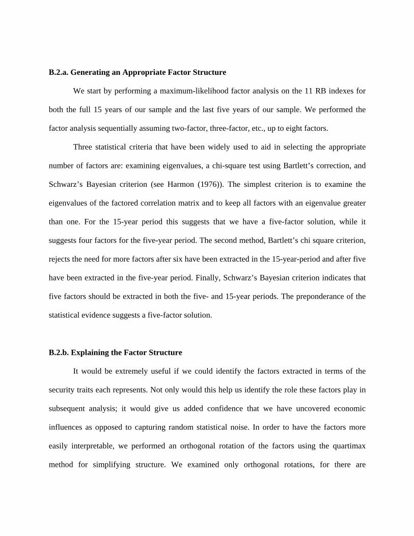
B.2.a. Generating an Appropriate Factor Structure

We start by performing a maximum-likelihood factor analysis on the 11 RB indexes for

both the full 15 years of our sample and the last five years of our sample. We performed the

factor analysis sequentially assuming two-factor, three-factor, etc., up to eight factors.

Three statistical criteria that have been widely used to aid in selecting the appropriate

number of factors are: examining eigenvalues, a chi-square test using Bartlett’s correction, and

Schwarz’s Bayesian criterion (see Harmon (1976)). The simplest criterion is to examine the

eigenvalues of the factored correlation matrix and to keep all factors with an eigenvalue greater

than one. For the 15-year period this suggests that we have a five-factor solution, while it

suggests four factors for the five-year period. The second method, Bartlett’s chi square criterion,

rejects the need for more factors after six have been extracted in the 15-year-period and after five

have been extracted in the five-year period. Finally, Schwarz’s Bayesian criterion indicates that

five factors should be extracted in both the five- and 15-year periods. The preponderance of the

statistical evidence suggests a five-factor solution.

B.2.b. Explaining the Factor Structure

It would be extremely useful if we could identify the factors extracted in terms of the

security traits each represents. Not only would this help us identify the role these factors play in

subsequent analysis; it would give us added confidence that we have uncovered economic

influences as opposed to capturing random statistical noise. In order to have the factors more

easily interpretable, we performed an orthogonal rotation of the factors using the quartimax

method for simplifying structure. We examined only orthogonal rotations, for there are

advantages in portfolio allocation and risk estimation in having an orthogonal set of indexes.

Quartimax rotation is an orthogonal rotation of the original factor solution such that each

variable has large factor loading with a small set of the rotated factors and small loading with the

rest.

In Table B1 we present the results of the quartimax rotation of the five-factor solution for

our 15-year sample. Each of the five factors has a reasonably straightforward interpretation. For

example, in the first factor all of the stock indexes with the exception of international stocks have

high loadings, while bond indexes, with the exception of high yield bonds, have extremely low

loadings. High-yield bonds and international stocks have intermediate loadings. This first rotated

factor can be clearly identified as a domestic stock factor. The two intermediate loadings can be

explained by the fact that high-yield bonds have stock-like characteristics and international

stocks, while different from domestic stocks, have some movement in common with domestic

stocks.

The second factor is clearly a domestic bond factor, while the third is an international

factor with both international bonds and stocks heavily loaded on it. The fourth and fifth factors

represent partitioning of domestic stocks into growth versus value and large versus small.

However, the division is not clean. Factor four has a lower loading on large growth than it would

if factor four was purely growth minus value. Thus factor four is growth minus value with a bias

against large growth stocks. Likewise, factor five is large minus small with a bias towards small

growth stocks.

We also performed a quartimax rotation for the five-year period, and the results were

similar to those presented in Table 4. Quartimax rotations were also examined for four- and six-

factor solutions over both the 15-year and 5-year periods, and the interpretation of the factors

was much less clear than the interpretation for the five-factor solution. This gave us added

confidence in our choice of five factors.

Factor analysis suggests that we need five indexes to approximate the original 11 indexes

in our data. However, this is based on the factors (indexes) containing short sales. Examining the

factor loadings shown in Table B1 indicates that if short sales were forbidden, at least two more

factors would be needed. These factors would represent large stocks and small stocks rather than

their difference, and value stocks and growth stocks rather than their differences. Based on this

analysis, if short sales of indexes are not allowed, we should expect to find that at least seven

indexes are needed to capture the security traits contained in our original eleven indexes.

B.3. Cluster Analysis

We now turn to cluster analysis to get further insight into how we can combine our

eleven indexes into a smaller set that captures the relevant information contained in the larger set

of indexes.

Cluster analysis is a series of routines that group elements, in this case indexes, into

groups based on how far apart they are in some space. There are several different ways distance

can be measured, and there are several different techniques that can be used for forming groups.

In this study we used three different distance measures and two clustering routines. The first

distance measure we used was difference in return space. Using returns as a distance measure,

cluster routines calculate the distance between two funds as the square root of the average

squared difference in monthly returns. The second distance measure normalizes the data so that

distance is measured in units of standard deviation. The third distance measure uses the

correlation between two funds or two groups as the measure of distance. Given alternative

distance measures, there remains the problem of how to proceed to combine firms.

We used two clustering algorithms to do this: the centroid method and Ward’s method. In

the centroid method, after two funds are combined, distance is calculated as if the two funds

become a single fund composed of an equally weighted average of the two funds. In the Ward

technique, distances are still calculated with respect to each of the funds within the group.

In each period examined (the 15-year period 1987-2001 and its three five-year sub-

periods) and for each clustering algorithm, the first three sets of indexes that combined were

mid-cap growth with small-cap growth (correlation 0.98), mid-cap value with small-cap value

(correlation 0.97), and government bond with mortgage bond (correlation 0.91). While these

correlation numbers are for the fifteen-year sample, five-year correlations are similar. The next

two indexes to enter a group were large-cap growth and large-cap value. Across all periods and

all clustering algorithms, two different patterns emerged. About half the time large-cap growth

and large-cap value first combined, followed by the small-cap and mid-cap growth combining

with small-cap and mid-cap value (size grouping). These size groupings then combined into one

overall domestic equity grouping. The other times the pattern was large-cap growth first

combining with the group small-cap and mid-cap growth and large-cap value combining with the

group small-cap and mid-cap value (value-growth groups), and then these two groups combining

into one overall domestic equity grouping at a later stage. World bond always joined the

combined government-corporate/mortgage bond group, and world equity always joined the

domestic equity group. In almost all circumstances high-yield bond joined the equity grouping.

The order with which high-yield bond and world equity joined domestic equity varied across

samples and the clustering algorithm used, with world equity usually the first. The last

combination was always bonds and stocks.

Their high correlation, their consistently combining in the first three steps in the process,

and the results from the factor analysis all provide strong evidence that we should combine three

pairs of indexes: small-cap growth with mid-cap growth, small-cap value with mid-cap value,

and government-corporate with mortgage bonds. Since the ordering of other clustering differs

across time periods and/or methodologies, we will proceed using the eight RB indexes that

remain after making these three combinations. As a final check, we repeated all of our tests in

section II comparing RB and OPB indexes using the eight RB indexes described above rather

than the eleven RB indexes. While there were small changes in the numbers, all of the results

were essentially unchanged except that one Sharpe ratio test was no longer significant.

Appendix C

In this appendix, we derive formulas for computing the average overall variance and

covariance when we know the average variance and covariance within each subgroup and the

average covariance between each pair of subgroups. Given estimates of the average variance for

each ICDI classification, then the average variance for the population, weighted proportional to

the holdings of our 417 sample 401K plans, is

∑∑ ⎟⎟

⎟⎟

⎠

⎞

⎜⎜⎜⎜

⎝

⎛

×=g

g

gg

g VarT

TVar (C1)

where

(1) is the total number of funds in ICDI group g held by the 401K plans (g = 1, …, 14); gT

(2) gVar is the average variance of funds in group g.

Given estimates of the average covariance within and between ICDI groups, the average

population covariance, if funds are selected using the weighted selection discussed in the text, is

( )

⎥⎥⎥⎥

⎦

⎤

⎢⎢⎢⎢

⎣

⎡

×+×−

×⎟⎠⎞

⎜⎝⎛= ∑ ∑∑

=≠==

G

g

G

gkk

gkkgG

gg

gg CovTTCovTT

XCov

1 11 211 (C2)

where

( )∑ ∑∑=

≠==

+−

=G

g

G

gkk

kgG

g

gg TTTT

X1 11 2

1

and

(1) gCov is the average covariance between funds in ICDI group g;

(2) gkCov is the average covariance between funds in ICDI group g and funds in ICDI

group k.

The average variance and average covariance for constrained random selection is done as

follows. The average variance and average covariance are computed as described above for the

set, which is a random stock fund and a random bond fund, and for a second set, which is

random selection for the whole population. The overall variance is computed using the standard

formula for a combination of two sets where the covariance between the sets is computed as

⎥⎥⎥⎥⎥

⎦

⎤

⎢⎢⎢⎢⎢

⎣

⎡

×+×+

⎥⎥⎥⎥⎥

⎦

⎤

⎢⎢⎢⎢⎢

⎣

⎡

×+×=

∑∑∑

∑∑

∑∑∑

∑∑

≠=

==

∈∈

≠=

==

∈∈

G

gkk

gkG

jj

kgG

jj

g

SgSg

g

g

G

gkk

gkG

jj

kgG

jj

g

BgBg

g

gPopBS

CovT

TCov

T

T

T

T

CovT

TCov

T

T

T

TCov

1

11

1

11

,

21

21

(C3)

where B is the set of ICDI domestic bond fund groups and S is the set of ICDI domestic stock

fund groups.

References

Agnew, Julie and Pierluigi Balduzzi, 2002, What do we do with our pension money? Recent evidence from 401K plans. Unpublished manuscript, Boston College. Bekaert, Geert and Michael S. Urias, 1996, Diversification, integration, and emerging market closed-end funds. Journal of Finance 51, 835-870. Benartzi, Shlomo and Richard Thaler, 2001, Naïve diversification strategies in retirement saving plans, American Economic Review 91(1), 78-98. Blake, Christopher R., Edwin J. Elton and Martin J. Gruber, 1993, The performance of bond mutual funds. Journal of Business. De Roon, Nijman and Werker, 2001, Testing for mean variance spanning with short sales constraints and transaction costs: the case of emerging markets. Journal of Finance 56(2), 721-742. De Santis, Giorgio, 1994, Asset pricing and portfolio diversification: Evidence from emerging financial markets. Working paper, University of Southern California. Elton, Edwin J. and Martin J. Gruber, 1970, Homogeneous groups and the testing of economic hypothesis. Journal of Financial and Quantitative Analysis. Elton, Edwin J. and Martin J. Gruber, 1977, Risk reduction and portfolio size: an analytical solution. Journal of Business 50, 415-434. Elton, Edwin J., Martin J. Gruber and Christopher R. Blake, 1996, The Persistence of Risk-Adjusted Mutual Fund performance. Journal of Business 69(2), 133-157. Elton, Edwin J., Martin J. Gruber and Christopher R. Blake, 1999, Common factors in fund returns. European Financial Review 3(1), 1-23. Elton, Edwin J., Martin J. Gruber and Christopher R. Blake, 2001, A first look at the accuracy of the CRSP mutual fund database and a comparison of the CRSP and Morningstar mutual fund databases. Journal of Finance 56(6). Elton, Edwin J., Martin J. Gruber and Jeffrey A. Busse, 2003, Are investors rational? Choices among index funds. Forthcoming, Journal of Finance. Fama, Eugene and Ken French, 1994, Book-to-market in earnings and returns, Journal of Finance. Gallant, A. Ronald, 1987, Nonlinear Statistical Models, John Wiley and Sons, New York.

Harman, Harry, 1976, Modern factor analysis. University of Chicago Press, Chicago, IL. Huberman, Gur and Shmuel Kandel, 1987, Mean-variance spanning, Journal of Fniance 42, 873-888. Huberman, Gur and Sengmuller, 2003, Company stock in 401K plans. Unpublished manuscript, Columbia University. Liang, Nellie and Scott Weisbenner, 2002, Investor behavior and the purchase of company stock in 401K plan design. Unpublished manuscript, University of Illinois. Lo, Andrew, 2002, The statistics of Sharpe ratios, Financial Analysts Journal 58, 36-50. Newey, W. and K. West, 1987, A simple positive definite heteroscedasticity and autocorrelation consistent covariance matrix, Econometrica 55, 703-705. Roll, Richard, 1977. A critique of the asset pricing theory’s tests, Journal of Financial Economics 4, 129-176.

Table 1

Percentages of 680 401K Plans O

ffering Different N

umbers of Investm

ent Choices

(Num

ber of choices and percentages include mutual funds, stable value funds, G

ICs and com

pany stock.)

Num

ber of Investment C

hoicesPercentage of Plans

12.21%

22.35%

33.09%

44.85%

58.97%

612.06%

712.06%

813.82%

911.76%

109.85%

115.59%

122.21%

132.50%

141.91%

151.18%

161.03%

17 or more

4.56%

e

Table 2

Types of Investm

ent Choices O

ffered in 680 401K Plans

Category

ICD

I Classification

Percentage of Plans Offering Investm

ent Choic

Interest Only

Money M

arket Fund57.35%

Stable Value Fund

24.85%G

IC14.71%

At Least O

ne Interest-Only Fund

86.76%

Dom

estic EquityA

ggressive Grow

th Fund55.44%

Grow

th and Income Fund; Equity Index

80.00%Long-Term

Grow

th Fund82.94%

Sector Fund6.47%

Total Return Fund; Equity V

alue Fund21.62%

Utilities Fund

0.59%A

t Least One D

omestic Equity Fund

97.35%

Dom

estic Bonds

Quality B

ond Fund54.85%

High-Y

ield Bond Fund

4.71%G

overnment M

ortgage Fund12.79%

Governm

ent Securities Fund12.35%

At Least O

ne Dom

estic Bond Fund

71.47%

Dom

estic Mixed

Balanced Fund

73.68%Incom

e Fund23.68%

At Least O

ne Dom

estic Mixed Fund

80.59%

InternationalG

lobal Bond Fund

9.12%G

lobal Equity Fund18.97%

Ineternational Equity Fund62.94%

At Least O

ne International Fund75.15%

Com

pany StockC

ompany Stock

22.94%

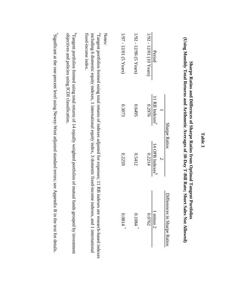
Table 3

Sharpe Ratios and D

iffernces of Sharpe Ratios from

Optim

al Tangent Portfolios

(Using M

onthly Total R

eturns and Arithm

etic Averages of 30-D

ay T-B

ill Rate; Short Sales N

ot Allow

ed)

Sharpe Ratios

Differences in Sharpe R

atios1

2Period

11 RB

Indexes a14 O

PB Indexes b

1 minus 2

1/92 - 12/01 (10 Years)

0.29760.2214

0.0762

1/92 - 12/96 (5 Years)

0.64950.5412

0.1084*

1/97 - 12/01 (5 Years)

0.30730.2259

0.0814*

Notes:

aTangent portfolios formed using total returns of indexes adjusted for expenses; 11 R

B indexes are research-based indexes

including 6 domestic equity indexes, 1 international equity index, 3 dom

estic fixed-income indexes, and 1 international

fixed-income index.

bTangent portfolios formed using total returns of 14 equally w

eighted portfolios of mutual funds grouped by investm

entobjectives and policies using IC

DI classification.

*Significant at the one-percent level using New

ey-West adjusted standard errors; see A

ppendix B in the text for details.

Table 4

Average V

ariances

The column labeled "Plan Funds" contains average variances assum

ing equal investment in each fund offered by a plan;

the column labeled "R

andom Selection" contains average variances assum

ing equal investment in funds random

ly selectedfrom

all funds in given ICD

I categories in the CR

SP mutual fund database, using as a probablity of selection in each IC

DI

category the proportion in that category held by the aggregate of all plans; the column labeled "constrained random

selection"contains average variances using the sam

e random selection as that for the previous colum

n, but with the constraint that the

first 2 funds selected are a bond fund and a stock fund.

Num

ber of Investment C

hoices in Plan aPlan Funds

Random

SelectionC

onstrained Random

Selection2

20.5123.36

10.893

16.2720.98

13.044

15.2919.79

13.975

16.0119.08

14.496

15.6318.61

14.827

17.6118.27

15.048

16.9918.01

15.219

17.7917.81

15.3310

17.2917.65

15.4311

16.8417.53

15.5112

17.9817.42

15.5713

13.7917.33

15.6214

15.5417.25

15.6715

14.8017.18

15.7116

16.1517.12

15.74

Note:

aExcluding company stock, m

oney market funds, G

ICs and stable value funds.

Table 5

Sufficiency of Plan Investment C

hoices in Spanning 8 RB

Indexes a

(Short Sales Not A

llowed)

Num

ber of Investment C

hoices in Plan bSufficient?

No

Yes

217

13

325

446

115

2825

642

167

2420

818

219

2322

106

811

47

127

413

11

141

315

07

160

6Total

249157

Notes:

aRB

indexes are research-based indexes including 4 domestic equity indexes, 1 international equity index,

2 domestic fixed-incom

e indexes, and 1 intrenational fixed-income index.

bExcluding company stock, m

oney market funds, G

ICs and stable value funds.

Table 6

Plan Characteristics G

rouped by Plan Asset Size D

eciles

Avg. Plan

Avg. N

umber

Percentage of PlansPercentage of Plans

Percentage of Plans Plan A

ssetA

sset Sizeof Investm

entthat U

se Sophisticated O

ffering Com

pany Stock Percentage of Plans

that Hire O

utsideSize D

ecile(Thousands)

Choices a

Strategies bas Investm

ent Choice b

that Vote Proxy

bC

onsultants b

1$2,124.579

4.4213.16%

7.89%13.16%

2.63%2

$6,045.9745.21

7.69%7.69%

7.69%5.13%

3$10,857.308

6.2110.26%

5.13%15.38%

5.13%4

$16,882.8215.23

7.69%20.51%

2.56%12.82%

5$24,754.590

6.0812.82%

20.51%7.69%

5.13%6

$37,363.9237.28

10.26%17.95%

12.82%23.08%

7$57,851.154

6.7217.95%

12.82%7.69%

28.21%8

$88,923.7187.82

20.51%38.46%

23.08%7.69%

9$173,890.667

7.8528.21%

41.03%15.38%

28.21%10

$780,277.8218.18

46.15%46.15%

17.95%20.51%

Spearman

Rank C

orr. b1.00

*0.95

*0.77

*0.84

*0.49

0.77*

Notes:

aExcluding company stock, m

oney market funds, G

ICs and stable value funds.

bSpearman rank correlation of decile colum

n with given colum

n; * = significant at 1% level.

cPercentages based on number of plans in size decile.

Table B1

Factor Loadings on 11 Indexes(Using Five-Factor Quartimax Rotation)

Type of Index Factor 1 Factor 2 Factor 3 Factor 4 Factor 5Large-cap Growth Stock 0.8704 0.0751 0.0445 0.0744 0.3628

Large-cap Value Stock 0.8912 0.1157 -0.0201 -0.3682 0.1408

Mid-cap Growth Stock 0.9214 -0.0380 0.0259 0.3285 0.1083

Mid-cap Value Stock 0.9183 -0.0521 -0.0554 -0.3261 -0.1478

Small-cap Growth Stock 0.9083 -0.0655 0.0003 0.4105 0.0252

Small-cap Value Stock 0.9335 0.0010 -0.0984 -0.1855 -0.2907

International Stock 0.5766 -0.0624 0.4687 -0.0258 0.1205

U.S. Bond 0.1099 0.9553 0.1029 -0.0085 -0.0167

Mortgage-Backed 0.1526 0.9332 0.0534 -0.0078 0.0193

High Yield Bond 0.5737 0.1993 -0.0624 0.0782 -0.2120

World Bond -0.0565 0.1899 0.9796 0.0134 -0.0294