The Accuracy of Television Network Rating Forecasts:

The Effects of Data Aggregation and Alternative Models

Dr Denny Meyer (*)

Faculty of Life and Social Sciences

Swinburne University of Technology

PO Box 218

Hawthorn VIC 3122

Australia

Ph: +61-3-92144824

Fax: +61-3-92148484

e-mail: dmeyer@swin.edu.au

Professor Rob J Hyndman

Department of Econometrics and Business Statistics,

Monash University, Australia

(*) Corresponding author

1

Abstract

This paper investigates the effect of aggregation in relation to the accuracy of

television network rating forecasts. We compare the forecast accuracy of network

ratings using population rating models, rating models for demographic/behavioural

segments and individual viewing behaviour models. Models are fitted using neural

networks, decision trees and regression. The most accurate forecasts are obtained by

aggregating forecasts from segment rating models, with neural networks being used to

fit these models. The resulting models allow for interactions between the variables

and the non-linear carry-over effect is found to be the most important predictor of

segment ratings, followed by time of day and then genre. The analysis differs from

those of previous authors in several important respects. The AC Nielsen panel data

considered stretches over 31 days, 24 hours per day, 60 minutes per hour, making it

necessary for ratings to be appropriately transformed prior to the fitting of the rating

models and for non-viewing time periods to be under-sampled when fitting the

models for individual viewing. For the first time individual viewing within each 15

minute time period is defined by network choice and proportion of viewing time.

Keywords: aggregation, discrete choice models, neural networks, decision trees, two-

stage models

1. Introduction

According to recent data published by AdWatch (2005), television advertising

makes up 44.8% of the total advertising spend in the United States of America.

Television executives sell time to advertisers at a price that is estimated using forecast

television network ratings; however, these audience projections are often made before

any program episodes have been aired. Forkan (1986) and Rust and Eechambadi

2

(1989) maintain that these forecasts have been very inaccurate in the past. Indeed,

Napoli (2001) has found that forecasting error has increased significantly over time.

Networks typically reschedule programs when actual audience sizes do not reach

projected levels. Advertisers are refunded when this happens, but they are not

compensated for the disruption to their media plan. Accurate forecasts are therefore

important and advertisers are prepared to pay for more reliable audience information

(Fournier and Martin 1983; Webster and Phalen 1997). This research adds to the

literature on improving the accuracy of short-term rating forecasts. In particular it

investigates the influence of forecast aggregation on forecast accuracy and the

importance of allowing for non-linearity and interaction effects when developing

rating models. It also investigates the relative importance of carry-over effects from

one time period to the next, genre, scheduling and audience segment in determining

rating forecasts.

Aggregation is an important research topic in time series analysis. A book on

temporal aggregation for ARMA processes written by Quenouille in 1957 is an early

example. More recently Granger and Lee (1999) have found that data aggregation

serves to simplify non-linearity while Tiao (1999) and Breitung and Swanson (2002)

have found that causality information is lost as a result of data aggregation, while

Zellner and Tobias (1999) have shown that data aggregation reduces forecasting

accuracy. In terms of agricultural economics Shumway and Davis (2001) claim that

inferential errors due to data aggregation are small relative to model estimation errors.

However, in other areas such as labour demand, it was found that aggregation bias

does occur (Lee et al, 1990). In this paper we consider the effect of aggregation on

forecasting accuracy for television ratings. The research question is “To what extent

should the data be aggregated before forecasting network ratings?”. Another way to

3

ask this question is “To what extent should forecasts for network ratings be

aggregated as an alternative to aggregation of the data prior to model estimation and

forecasting?”.

Linear regression models for the prediction of population ratings have been used

by several authors (Barwise and Ehrenberg, 1984, 1988; Reddy et al, 1996; Kelton

and Stone, 1998). These models are all short-term in nature, being typically derived

from prime time viewing for only a few weeks of the year, often only one week, using

AC Nielson panel data for viewing in 15 minute or 30 minute periods. Most of these

rating models have considered network, time of day, day of the week, and the rating

for the previous period as the predictor variables in their models. However, Shachar

and Emerson (2000) have incorporated program dummies, cast demographics and

switching costs in their rating models.

The fitting of such rating models has been criticised by Rust and Eechambadi

(1989) because audience demographics are not taken into account. In answer to this

criticism several authors have used choice models (nominal logistic regression) to

analyse individual network choices, obtaining ratings by aggregating the predictions

from their models (Rust and Eechambadi 1989; Swann and Tavakoli 1994, Tavakoli

and Cave 1996; Shachar and Emerson 2000; Goettler and Shachar 2001;).

Alternatively, some authors have included a behavioural and/or demographic segment

in their model with Rust et al (1992) recommending that segments with homogeneous

viewing are preferable to a segmentation based on demographics or life style. These

authors developed network choice models for each of three demographic/geographic

segments and then combined the predicted network probabilities for each segment

using the relative size of each segment as a weight.

4

Models for individual network choice have also included network, time of day, day

of the week and genre. All the above models for network choice are fitted using

logistic regression methods. Swann and Tavakoli (1994) allow for interactions

between program genre and demographics (gender, age and socio-economic level)

with product terms and, in the same way, Kelton and Stone (1998) allow for genre

interactions with time of day and day of the week.

There is clearly a large literature dealing with models for television viewing.

However, there are some notable omissions from this literature. Interestingly, perhaps

on account of the emphasis on prime time viewing, the distribution of rating model

errors is assumed normally distributed despite the fact that ratings are proportions and

therefore heteroscedastic. It is expected that an arcsine square root transformation will

produce more reliable rating models while still allowing for zero ratings (Sokal and

Rohlf, 1969, p386). All authors appear to ignore the relatively high percentage of non-

viewer records in the data sets used to estimate network choice models for individuals.

In our data set the percentage of records for non-viewers was nearly 90%. In these

circumstances it is necessary to under-sample the non-viewers or over-sample the

viewers for each time period in order to obtain reliable models (Berry and Linoff,

1997, p.78). Our models learn by example so we need a reasonable proportion of

cases in each of the categories of interest.

In addition it appears that no authors have made allowance for network switching

within a time period, perhaps because they did not have this information. Also there is

no comparison of the performance of non-linear models fitted using decision trees or

neural networks with the performance of simpler models fitted using regression or

logistic regression. Finally, to the best of the authors’ knowledge the literature

contains no comparison of the accuracy of rating forecasts obtained from data at

5

different aggregation levels (e.g. population, segment or individual). This paper

addresses these issues directly while investigating the following expectations in the

current context.

1) It is expected that for rating models neural networks will perform best because they

allow for interaction effects and for any non-linear rating carry-over effects from one

period to the next. Despite their ability to model interaction effects, trees are not

expected to manage the carry-over effect as well as neural networks, requiring too

many branches in order to achieve the same accuracy as neural networks. Regression

models are expected to perform worse than neural networks when they are not

specifically designed to describe interaction effects or non-linear effects.

2) For individual viewing models it is expected that decision trees will provide more

than neural networks or regression models. The independent variables in this case are

all nominal, allowing the use of relatively simple trees to describe interaction effects.

Again regression models must be specifically designed to incorporate these

interactions, while the power of neural network models in describing non-linear

relationship is not utilised in these models.

3) In all our models, carry-over effects from one time period to the next are expected

to be most important predictors. Genre is expected to be an important predictor only

for the individual viewing models, with genre effects obscured when ratings are

considered.

4) It is expected that the population rating forecasts will be relatively inaccurate

because no demographic information is used while forecasts based on individual

viewing will also be relatively inaccurate because of idiosyncratic individual

behaviour. The most accurate rating predictions are therefore expected from the

6

aggregated segment forecasts. In addition the segment forecasts will allow advertisers

to better match their advertising to their audiences.

This paper is expected to advance our understanding of rating prediction on several

fronts. Firstly, it will compare the accuracy of three model estimation tools

(regression, neural networks and decision trees) in the context of television rating

models. Secondly it will determine the relative importance of the predictor variables

(genre, time of day, network, carry-over, demographic/viewing segment) in rating

predictions. Finally it will compare the accuracy of three aggregation strategies for

rating forecasts.

2. Methodology

This study predicts TV ratings from individual viewing and demographic data,

collected in New Zealand by Nielsen Media Research during July 2003. The data

were recorded by people meters located in 470 households containing approximately

1226 people. We consider viewing data for 15 minute time periods, only the 3 most

popular networks (TV1, TV2 and TV3) and 14 program genres. In all there were

approximately 3.2 million records of individual data that were compressed into ratings

for 2976 fifteen minute time periods for each of the three networks. Ratings were

calculated for each of these time periods taking into account the viewing time for each

person in the panel (as a fraction of 15 minutes) and the weight assigned to each

person by AC Nielsen Media Research. If the panel were to reflect the demographics

of the New Zealand population exactly all these weights would be one. In practise this

is not possible so people in the panel must be weighted more highly if they have

demographic characteristics that are under represented in the panel, while people

7

whose demographic characteristics are over represented in the panel must be weighted

lower. These weights must of course sum to one for each time period.

The formula used to calculate these ratings is given below in (1). If we define Vkjt

as the proportion of viewing time for individual k on network j in time period t and

Wkt as the weighting for individual k in time period t, then we can calculate Rjt, the

rating for network j in time period t, by summing over all n individuals who view

network j in time period t.

∑=

=n

kkjtktjt VWR

1* (1)

Population rating models were derived using ratings for the 2976 fifteen minute

time periods for each of the three networks. In view of the size of our data sets,

standard data mining approaches, as described in Berry and Linoff (1997), were

applied in the fitting and testing of models. Models were fitted, validated and tested

using independent samples of appropriate size and composition. Forty percent of the

data was used for training, 30% was used as a validation data set in order to prevent

overfitting and error variances were estimated using a 30% holdout (test) sample. The

models for individual viewing were derived using a data set describing individual

behaviour in each of the 2976 time periods. However, time periods when individuals

were not viewing networks TV1, TV2 or TV3 were under-sampled in order to provide

a more balanced data set in terms of network choice. In these “non-viewing” time

periods there was either no viewing or the chosen network was not TV1, TV2 or TV3.

Only 6% of the “non-viewing” time periods were selected using a systematic sample,

after sorting the data by day of the month and time of day. The reduced data set,

consisting of 562 thousand observations, contained 31% TV1, 22% TV2, 18% TV3

and 29% “Nonviewer” records.

8

Variable Transformation. In order to avoid heteroscedasticity in the residuals the

ratings were transformed using the arcsine square root transformation. This

transformation is recommended for responses that are proportions as explained

previously (Sokal and Rholf, 1969). In addition the genre and time of day variables

were collapsed into fewer categories by the Enterprise Miner variable selection node.

This node collapses the categories in such a way as to maximise the correlation with

the dependent variables. This meant that the number of genre and time of day

categories varied in response to changes in the dependent variable. In the case of the

14 genre categories, five collapsed genre categories were normally used while the 96

fifteen minute time of day blocks were usually replaced by only six time of day

categories. This reduction in the number of categories for the genre and time of day

variables served to simplify all our models, thereby improving predictive accuracy.

Model Estimation. All analyses were performed using SAS or SAS Enterprise

Miner. A simple least squares approach was used to fit all the models except the

individual network choice models. We allowed for network switching within a time

period by fitting individual network choice models and the proportion of viewing time

models simultaneously, using a two-stage procedure (Amemiya, 1974), with the

network choice probabilities, in particular the probability of the “nonviewing”

network, incorporated in the proportion of viewing time model. This approach

permitted correlation between probabilities for network choice and proportion of

viewing time, with higher times expected for the “nonviewing” network.

Types of model. Neural networks, decision trees and regression models have been

used to estimate our models. Multilayer perceptrons, described by Bishop (1995),

provided the architecture for the neural networks with hyperbolic tangent functions

producing values for a single layer of hidden nodes and linear functions producing

9

output values. F-tests were used to determine the optimum splitting points when

producing decision tree models (Breiman et al, 1984). CHAID decision trees, first

published by Hartigan (1975), with chi-squared tests to obtain the optimum splitting

points, were used for predicting network choice. In all trees only binary splits were

permitted. A backward selection of variables was used in the estimation of the

regression models and there was no attempt to incorporate interaction terms in these

models.

Population Rating Model Approach. The rating for network j in time period t as

defined in (1) can be described in terms of a set of dummy variables for network,

genre, day of the week and time of day as well as carryover effects, measured using

lagged terms for the previous period’s rating, and random error (e). The f(.) function

represents an arcsine square root transformation, used to ensure that the random errors

have a more constant variance and a more normal distribution, while the Greek letters

(α, δ, γ, β, η, τ) represent parameters that must be estimated. The dummy variables are

defined with Njt set equal to one for network j in time period t, Gjxt set equal to one for

genre x showing on network j in time period t, Drt set equal to one for time t on day r

and Bqt set equal to one for time of day category q in time period t.

jtq

qtqr

rtrx

jxtxjtjtjjt eBDGNRRf +∑+∑+∑+++= − τηβγδα 1,)( (2)

However, the predictions from this model need to be constrained to allow for the

choice nature of television viewing and the competition between the networks. As

observed by Webster and Lichty (1991), Patelis et al. (2003) and others, a better way

to estimate ratings is to first obtain predicted television ratings for period t ( tR ) and

then multiply by the estimated network shares for each network j for time period t

( jtS ) to obtain a constrained predicted network rating for each network j for time

10

period t ( jtR ). Model (3) can be used to estimate the overall television rating for all

networks with the constrained network ratings calculated from (4). In model (3) the

Greek letters (φ, ϕ, and θ) must be estimated while Drt and Bqt are defined as for (2)

and the error term is denoted by at.

tq

qtqr

rtrtt aBDRRf +∑+∑++= − θϕφα 1)( (3)

jtt

llt

jttjt SR

R

RRR ˆˆ

ˆ

ˆˆˆ

3

1

=∑

=

=

(4)

If models (2) and (3) are fitted using regression trees or neural networks, non-linear

carry-over effects and factor interactions can be automatically included.

Segmentation. It was expected that more accurate rating forecasts could be

obtained by splitting the people in the AC Nielsen panel into segments with similar

demographics and viewing behaviour, and then developing separate rating models for

each segment. The dendogram from an agglomerative hierarchical segmentation was

constructed using Ward’s linkage method (Hair et al, 1998, p. 496). Four segments

loosely defined in terms of age and viewing behaviour were suggested and the

characteristics of these segments are described in Table 1. The first segment was the

largest, containing mostly middle-aged people, while the second segment contained

mostly young people under the age of twenty. The third segment had a large

percentage of retired people while the fourth segment contained a high percentage of

people who watch other networks, in particular the SKY networks, which unlike TV1,

TV2 and TV3 have a monthly rental.

Place Table 1 about here

Segment Rating Model Approach. The above models (2) and (3) can also be

developed for each of the four segments (i=1,2,3,4), and the rating forecasts ( ijtR )

11

from these four models can then be aggregated to provide an alternative population

rating forecast for each network j in each time period t. Following the approach of

Rust et al (1992), if the weight for the ith segment is ωi, with ∑=

=4

11

iiω , we obtain

estimated ratings for network j by summing over the four segments as shown below.

ijti

ijt RR ˆˆ4

1∑=

= ϖ (5)

Individual Viewing Model Approach. The forecasts from the individual viewing

models can also be aggregated to provide a further population rating forecast for each

network in each time period. We use Discrete Choice Models to describe the network

choices of an individual, including “No Viewing” as one of the networks. Possible

input variables include day of the week (D), time of day (B), demographic

characteristics as measured by the segmentation category (C), program genre (G) and

carry-over viewing behaviour from the network viewed in the previous time period.

All these variables are nominal and must therefore be recoded using sets of dummy

variables. The target variable was the individual network choice. This model can be

fitted using conventional logistic regression analyses or it can be fitted using

classification trees or neural network analyses if interaction effects are to be included.

Assuming that network 4 is the “No Viewing” network choice, we define Pkjt as

the probability that individual k will watch network j during time period t. Then

kjtq

qtqr

rtrx

jxtxi

iitjjtkkjt rBDGCNPP +∑+∑+∑+∑++= − ζυψξκν 1,4 )/ln( (6)

In this model the Greek letters (ν, κ, ξ, ψ, υ and ζ) are parameters which must be

estimated and rkjt is the error term. The variable Ci is set equal to one if person k

belongs to segment i, zero otherwise, and the other variables (N, G, D and B) are

dummy variables defined as in (2). In fitting this model we are assuming that all

12

viewers can choose among all available networks but can choose only one of these

networks to view in any time period. This assumption was obviously false for our 15

minute periods because people often switch networks inside a 15 minute period. We

therefore also needed to estimate the proportion of time spent viewing any network

and we needed to distribute the weights for each person between the networks in

accordance with this proportion when predicting ratings.

Viewing time for network j by person k in time period t is expressed as a

proportion of the possible 15 minutes in any time period. Models for this variable

(Tkjt) have a similar form to (6) above, but the estimated probabilities for network

choice ( kjtP ) were also included as predictor variables, necessitating the use of a Two-

Stage procedure for fitting the kjtP and kjtT models simultaneously. Estimated viewing

time proportions were then adjusted proportionately in order to ensure that they added

to one for every 15 minute time period. Forecasts for kjtP and kjtT ( kjtP and kjtT ) were

easily converted into estimated ratings ( jtR ) for network j at time interval t using the

following formula.

∑==

jtn

kktkjtkjtjt WTPR

1

ˆˆˆ (7)

where Wkt is the individual k weighting in time period t and njt is the number of

network j viewers at this time.

Forecast Aggregation. Three levels of forecast aggregation were considered for

the production of network ratings, with higher levels of data aggregation

corresponding to lower levels of forecast aggregation (if any). Firstly, in the case of

the models for population ratings in (3) above, there was no need to aggregate

forecasts because the data used for the model had already been fully aggregated in the

form of population network ratings.

13

Secondly, when separate network rating models were fitted for each of the

segments, the segment forecasts had to be aggregated across the four segments in

order to produce forecasts for network ratings. In this case there was initial

aggregation of the data in order to produce segment ratings and then further

aggregation of the forecasts across the segments in order to produce population

network ratings. As indicated in (5) above each segment forecast was weighted

according to the size of the segment before this final aggregation took place.

Thirdly, models for individual viewing behaviour were fitted for all the

individuals in the panel, producing individual forecasts for network choice and

viewing time within each time period. In this case there was no data aggregation so

maximum forecast aggregation was required in (7) above in order to produce

population network ratings while taking into account the AC Nielsen weights assigned

to each person.

Relative Importance of Predictors and Predictive Accuracy. For each of the

above models the relative importance of the predictor variables was assessed using an

R-square contribution in the case of the rating and proportion of time models and

using a normed chi-square value contribution ( df/2χ ) in the case of individual

network choice. Variables which contribute more of the explanatory power in a model

are considered to be more important.

Finally, in this study predictive accuracy is measured using expected bias, error

standard deviations, mean absolute error and mean absolute error. In particular,

models which produce lower mean square errors are preferred to models which

produce higher mean square errors. Wherever possible errors are calculated from

hold-out (test) samples rather than just the data used to fit the models.

14

3. Results

In this section we fit the various models using neural networks, decision trees and

regression, choosing the best fitting models in terms of the test data to provide our

rating forecasts for each network in each time period. We then compare the above

three aggregation approaches using the complete data for July 2003 to compute the

average squared prediction errors.

As expected it was found that the residuals for the rating models were well

behaved, exhibiting homoscedasticity as a result of the arcsine square root

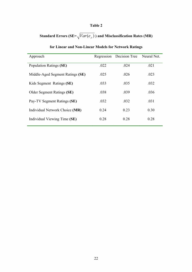
transformation and randomness. The results in Table 2 show the standard errors for

the test data when the models described in (2) and (6) were fitted to the data. Note that

the standard errors for the rating models were defined in terms of the transformed

ratings while the standard errors for the viewing time model were defined as a

proportion of a 15 minute time period. The neural network models were fitted using 2,

3 and 4 hidden nodes with the best results, usually for 3 hidden nodes, reported in

Table 2.

The results were remarkably similar for regression, decision trees and neural

networks suggesting that it does not much matter which type of model is used.

However, as expected, the population and segment rating models were a little more

accurate when fitted using neural networks, suggesting that there are non-linear carry-

over effects and interactions. Also, as expected, the models for network choice were a

little more accurate when decision trees were used for handling the interaction effects

for the nominal predictors. However, there were no obvious differences in the case of

the individual viewing time models.

Interestingly the results for the total population and for the “Middle-Aged”

segment were better than the results for the “Kid”, “Older” and “PayTV” segments.

15

There was a moderate positive correlation between the forecast errors for the

“Middle-Aged” and “Kids” segments (r = 0.57), suggesting underlying environmental

effects not captured in the explanatory variables in these models. However, the

forecast errors for the “Older” segment showed a strong negative correlation with the

forecast errors for the “Middle-Aged” and “Kids” segments (r = -0.76 and r = -0.73),

suggesting improved accuracy for a stratified forecast based on all four segments,

with positive errors for the “Middle-Aged” and “Kids” segments cancelled by

negative errors for the “Older” segment.

Place Table 2 about here

Table 3 compares the results for the best of the above models when applied to the

whole data set. In this case errors were computed from the untransformed rating data

allowing a comparison of the three different aggregation approaches. As expected

from the error correlations for the segment forecasts, the aggregation of segment

ratings produced a good result. Despite the larger bias in the aggregated segment

forecast, the error standard deviation is small producing the lowest mean square error.

This was confirmed by the average relative absolute errors, computed by ignoring all

zero ratings, and the mean absolute errors, suggesting that this approach will produce

the best results on average. A comparison of the population rating forecasts and the

aggregated individual viewing forecasts showed mixed results in terms of the various

error measures, with a higher MSE but lower MAE and MARE for the population

rating forecasts.

Place Table 3 about here

Next we consider the relative importance of the predictor variables in each of the

models. Strangely, day of the week was not a significant variable in any of the models

and was therefore dropped. As shown in Table 4, the carry-over effect was the most

16

important predictor variable for all the models except viewing time. For the

population and segment rating models time of day was more important than genre.

However, genre and segment were more important than time of day in the case of

individual network choice models. Clearly the importance of genre was obscured

when more aggregated data models were used. The model for individual viewing time

within each 15 minute time period was somewhat disappointing, explaining only a

small proportion of the variation in this variable.

Place Table 4 about here

4. Conclusions

Three aggregation approaches have been used to forecast television program

ratings, with trees and neural network fitting procedures used in order to allow for

interactions between the input variables and for non-linear relationships. A carry-over

effect from the previous time period was the most important predictor, with time of

day relatively important in the rating models and genre and segment more important

in the network choice model. For all levels of aggregation linear regression models

tended to perform worse than neural networks or trees when interaction effects and/or

non-linear carryover were ignored. Neural networks performed best in the case of

rating models while decision trees performed best in the case of the individual

viewing models.

The results suggested that the best forecast accuracy is obtained from segment

rating models, using a weighted average of the segment forecasts. This suggests that

aggregation bias will be small provided that sufficient demographic data is

incorporated via the segmentation. It is recommended that this approach be used to

produce the rating forecasts required by program schedulers and advertisers, with

neural networks being used to fit these models. In addition it is recommended that an

17

arcsine square root transformation be applied to the ratings in order to ensure that

model errors show homoscedastic behaviour.

However, the above models are based on data only for July 2003 and it is well

known in the television industry that television viewing is affected by economic

cycles and the seasons. In order for a television rating forecast to be useful to program

schedulers the model would need to be fitted to recent appropriate data (say last

month’s data) in order to obtain reasonably accurate forecasts and prediction intervals.

Alternatively the model needs to include a time and a seasonal dimension as

suggested by Gensch and Shaman (1980), Patelis et al. (2003). A third approach is to

build separate models for every successive month and to produce rating estimates and

standard errors from each of these models. Reliable forecasts for program ratings

and their standard errors can then be obtained from these time series using methods

such as exponential smoothing or time series decomposition.

Finally, as recommended by Patelis et al. (2003), rating forecasts need to be

supported by a Decision Support System which incorporates qualitative factors for the

forecasting of television viewership. Such a system should allow easy access to

information and “what if” queries as well as the entry of exceptional influence

impacts on television viewing.

Acknowledgements Our sincere thanks to AGB Nielsen Media Research for providing us with the data that has made this study possible.

18

References

AdWatch (2005). 3/4/06. http://www.tns-mi.com/downloads/res_adWatch2005.ppt#8

Amemiya, T. (1974), The Nonlinear Two-stage Least-squares Estimator, Journal of

Econometrics, 2, 105-110.

Barwise, P. & A. Ehrenberg. (1984), The reach of TV channels. International Journal

of Research in Marketing 1: 37-49.

Barwise, P. & A. Ehrenberg. (1988), Television and its Audience. Sage Publications:

London.

Berry, M.J.A. & Gordon Linoff, (1997), Data Mining Techniques. New York: Wiley .

Bishop, C.M. (1995), Neural Networks for Pattern Recognition, Oxford: Oxford

University Press.

Breiman, L., Friedman, J., Olshen, R. & Stone, C (1984), Classification and

Regression Trees. Wadsworth.

Breitung, J. & N.R. Swanson (2002), Temporal Aggregation and Spurious

Instantaneous Causality in Multiple Time Series Models. Journal of Time Series

Analysis 23(6): 651-65.

Forkan, J.P. (1986), Nielsen Waters Down TV Forecasters’ Tea Leaves. Advertising

Age, (April 7), 24:79.

Fournier, G.M. & D.L. Martin (1983), Does Government-Restricted Entry Produce

Market Power? New Evidence from the Market for Television Advertising. Bell

Journal of Economics, 14 (Spring): 44-56.

Gensch, D. & P. Shaman. (1980), Models of Competitive Television Ratings. Journal

of Marketing Research 17(3): 307-15.

Goetler, R.L. & R. Shachar (2001), Spatial competition in the network television

industry. RAND Journal of Economics 32(4): 624-656.

19

Granger, C.W.J. & T.H. Lee (1999), The Effect of Aggregation on Nonlinearity.

Econometrics Reviews 18(3): 259-69.

Hair, J.F., R.E. Anderson, R.L. Tatham & W.C. Black (1998), Multivariate Data

Analysis. Prentice-Hall: New Jersey

Hartigan, J.A. (1975), Clustering Algorithms. Wiley: New York.

Kelton, C.M.L. & L.G.S. Stone (1998), Optimal television schedules in alternative

competitive environments. European Journal of Operational Research, 104, 451-

473.

Lee, K.C., M.H. Pesaran & R.G. Pierse (1990), The Aggregation Bias in Labour

Demand Equations for the UK Economy. Routledge: London and New York.

Napoli, P.M. (2001), The Unpredictable Audience: An Exploratory Analysis of

Forecasting Error for New Prime-Time Network Television Programs. Journal of

Advertising 30(2): 53-101.

Patelis, A., K. Metaxiotis, K. Nikolopoulos & V.Assimakopoulos (2003), FORTV:

Decision Support System for Forecasting Television Viewership. Journal of

Computer Information Systems 43(4): 100-107.

Quenouille, M.H. (1957), The Analysis of Multiple Time Series. London:Griffin.

Reddy, S.K., J.E. Aronson & A. Stam (1996), SPOT: Scheduling Programs Optimally

for Television. http://citeseer.nj.nec.com/cache/papers/cs/14141/ [2nd March 2004].

Rust, R.T. & N.V. Eechambadi (1989), Scheduling Network Television Programs: A

Heuristic Audience Flow Approach to Maximising Audience Share, Journal of

Advertising 18(2): 11-18.

Rust, R.T., W.A. Kamakura & M.I. Alpert (1992), Viewer Preference Segmentation

and Viewing Choice Models for Network televisions, Journal of Advertising 21(1):

1-18.

20

Shachar, R. & J.W. Emerson (2000), Cast Demographics, Unobserved Segments, and

Heterogeneous Switching Costs in a Television Viewing Choice Model, Journal of

Marketing Research 37(2): 173-186.

Shumway, R. & G.C. Davis (2001), Does consistent aggregation really matter? The

Australian Journal of Agriculture and Resource Economics 45(2): 161-94.

Sokal, R.R. and F.J. Rohlf (1969), Biometry: The principles and practise of statistics

in biological research. W.H. Freeman and Company: San Francisco.

Swann, P. & M.Tavakoli (1994), An econometric analysis of television viewing and

the welfare economics of introducing an additional channel in the UK. Information

and Economics Policy 6: 25-51.

Tavakoli, M. & M. Cave (1996), Modelling Television Viewing Patterns. Journal of

Advertising 25(4): 71-86.

Tiao, G.C. (1999), The ET interview: Professor George C. Tiao. Econometric Theory

15: 389-424.

Webster, J.G. & L.W. Lichty (1991), Ratings Analysis: Theory and Practice.

Lawrence Erlbaum: Hillsdale, NJ.

Webster, J.G. & P. F. Phalen (1997), The Mass Audience: Rediscovering the

Dominant Model, Mahwah, NJ: Lawrence Erlbaum Associates.

Zellner, A.& J. Tobias (1999), A Note on Aggregation, Disaggregation and

Forecasting Performance. Research Report June 1. Graduate School of Business,

University of Chicago.

21

Table 1

Segment Characteristics

Segment 1 2 3 4 All % Viewers 38.0 14.5 28.1 19.4 100 Favourite network TV2 TV2 TV1 TV1 TV1 Average Daily Viewing(hrs)

2.3 1.8 3.0 2.2 2.4

% under 20 years 21.5 91.4 3.8 19.6 26.3 % 20 – 60 years 71.5 8.6 53.9 62.6 55.7 % 60+ years 7.0 0.0 42.3 17.8 18.0 % SKY viewing 1.9 2.2 1.9 34.1 8.2 % viewing 5pm-8pm 30.8 35.5 45.0 33.2 35.9 %viewing 8pm-11pm 40.3 18.3 35.3 34.7 34.6 %viewing 8am-5pm 18.1 39.6 15.9 21.7 21.3 % Male 49.8 57.7 33.1 57.5 47.7 % University Graduate 14.3 1.8 14.8 12.8 11.3 % European Descent 60.3 50.3 81.4 62.1 65.1 % without income 7.0 35.6 2.8 2.7 9.1 % income >$50000 12.4 0.0 13.3 23.3 13.0 Segment Name Middle-

Aged Kids Older Pay-TV

Patrons Complete

Panel

22

Table 2

Standard Errors (SE= )( jteVar ) and Misclassification Rates (MR)

for Linear and Non-Linear Models for Network Ratings

Approach Regression Decision Tree Neural Net.

Population Ratings (SE) .022 .024 .021

Middle-Aged Segment Ratings (SE) .025 .026 .023

Kids Segment Ratings (SE) .033 .035 .032

Older Segment Ratings (SE) .038 .039 .036

Pay-TV Segment Ratings (SE) .032 .032 .031

Individual Network Choice (MR) 0.24 0.23 0.30

Individual Viewing Time (SE) 0.28 0.28 0.28

23

Table 3

Effect of Forecast Aggregation on Prediction Accuracy for Network Ratings

MSE: Mean Squared Error; MAE: Mean Absolute Error;

MARE: Mean Absolute Relative Error

Aggregation Level

for forecasts

Expected

Bias

Error

StdDev

MSE MAE MARE

No aggregation

Population Ratings

0.107 1.299 1.698 0.648 0.418

Aggregation of

Segment Ratings

0.263 1.022 1.114 0.536 0.275

Aggregation of

Individual Viewing

0.174 1.216 1.508 0.726 0.939

24

Table 4

Predictor Importance Based on Percentage Variation Explained

(Normed Chi-Square for Network Choice, R-Square otherwise)

Segment Ratings for

segment categories:-

Predictors Population

Ratings

1 2 3 4

Network

Choice

(Pijk)

Time

(Tijk)

Carry-over Rating .95 .94 .91 .94 .91 n.a.

Carry-over Network n.a. n.a. n.a. n.a. n.a. 5484.17 0.01

Time of day (B) .78 .75 .55 .56 .61 40.91 0.06

Genre (G) .20 .24 .23 .20 .19 634.76 0.13

Network Choice (N) .04 .03 .10 .19 .08 n.a. 0.13

Segment Category(C) n.a. n.a. n.a. n.a. n.a. 814.17 <0.01